Algorithms and Abstract Data Types Informally, algorithm means is a well-defined computational procedure that takes some value, or set of values, as input and produces some other value, or set of values, as output. An algorithm is thus a sequence of computational steps that transform the input into the output. Algorithm is also viewed as a tool for solving a well-specified problem, involving computers. The statement of the problem specifies in general terms the desired input/output relationship. The algorithm describes a specific computational procedure for achieving that input/output relationship. There exist many points of view to algorithms. One if these points is a computational one. A good example of this is a famous Euclid’s algorithm: for two integers x, y calculate the greatest common divisor gcd (x, y) Direct implementation of the algorithm looks like: program euclid (input, output); var x,y: integer; function gcd (u,v: integer): integer; var t: integer; begin repeat if u<v then begin t := u; u := v; v := t end; u := u-v; until u = 0; gcd := v end; begin while not eof do begin readln (x, y); if (x>0) and (y>0) then writeln (x, y, gcd (x, y)) end; end. This algorithm has some exceptional features, nevertheless specific to the computational procedures: • it is computationally intensive (uses a lot of processor mathematical instructions); • it is applicable only to numbers; • it has to be changed every time when something of the environment changes, say if numbers

are very long and does not fit into a size of variable (numbers like 1000! – see picture below). For algorithms of applications in the focus of this course, like databases, information systems, etc., they are usually understood in a slightly different way, more like tools to achieve input/output relationship. The example of an algorithm in such sense would be a sorting procedure. This procedure is frequently appearing in a transaction (a prime operation in information systems or databases), and even while the same transaction, the sorting: • is repeated many times; • in a various circumstancies; • with different types of data.

• 402387260077093773543702433923003985719374864210↵714632543799910429938512398629020592044208486969↵404800479988610197196058631666872994808558901323↵829669944590997424504087073759918823627727188732↵519779505950995276120874975462497043601418278094↵646496291056393887437886487337119181045825783647↵849977012476632889835955735432513185323958463075↵557409114262417474349347553428646576611667797396↵668820291207379143853719588249808126867838374559↵731746136085379534524221586593201928090878297308↵431392844403281231558611036976801357304216168747↵609675871348312025478589320767169132448426236131↵412508780208000261683151027341827977704784635868↵170164365024153691398281264810213092761244896359↵928705114964975419909342221566832572080821333186↵116811553615836546984046708975602900950537616475↵847728421889679646244945160765353408198901385442↵487984959953319101723355556602139450399736280750↵137837615307127761926849034352625200015888535147↵331611702103968175921510907788019393178114194545↵257223865541461062892187960223838971476088506276↵862967146674697562911234082439208160153780889893↵964518263243671616762179168909779911903754031274↵622289988005195444414282012187361745992642956581↵746628302955570299024324153181617210465832036786↵906117260158783520751516284225540265170483304226↵143974286933061690897968482590125458327168226458↵066526769958652682272807075781391858178889652208↵164348344825993266043367660176999612831860788386↵150279465955131156552036093988180612138558600301↵435694527224206344631797460594682573103790084024↵432438465657245014402821885252470935190620929023↵136493273497565513958720559654228749774011413346↵962715422845862377387538230483865688976461927383↵814900140767310446640259899490222221765904339901↵886018566526485061799702356193897017860040811889↵729918311021171229845901641921068884387121855646↵124960798722908519296819372388642614839657382291↵123125024186649353143970137428531926649875337218↵940694281434118520158014123344828015051399694290↵153483077644569099073152433278288269864602789864↵321139083506217095002597389863554277196742822248↵757586765752344220207573630569498825087968928162↵753848863396909959826280956121450994871701244516↵461260379029309120889086942028510640182154399457↵156805941872748998094254742173582401063677404595↵741785160829230135358081840096996372524230560855↵903700624271243416909004153690105933983835777939↵410970027753472000000000000000000000000000000000↵000000000000000000000000000000000000000000000000↵000000000000000000000000000000000000000000000000↵000000000000000000000000000000000000000000000000↵000000000000000000000000000000000000000000000000↵000000000000000000000000

Pseudocode The notation language to describe algorithms is needed. This language called pseudocode, often is a lingua franca. Pseudocode is used to express algorithms in a manner that is independent of a particular programming language. The prefix pseudo is used to emphasize that this code is not meant to be compiled and executed on a computer. The reason for using pseudocode is that it allows one to convey basic ideas about an algorithm in general terms. Once programmers understand the algorithm being expressed by pseudocode, they can implement the algorithm in the programming language of their choice. This, in essence, is the difference between pseudocode and a computer program. A pseudocode program simply states the steps necessary to perform some computation, while the corresponding computer program is the translation of these steps into the syntax of a particular programming language. Kind of mixed sentences, expressions, etc. derived from Pascal, from C, and from JAVA (sometimes) will be used to express algorithms. There will be no worry about how the algorithm will be implemented. This ability to ignore implementation details when using pseudocode will facilitate analysis by allowing us to focus solely on the computational or behavioural aspects of an algorithm. Constructs of pseudocode: • assignments; • for … to … [step] … do [in steps of]; • while … do; • do … while; • begin … end; • if … then … else; • pointer, and null pointer; • arrays; • composite data types; • procedure and its name; • formal parameters versus actual parameters.

Abstract Data Types A theoretical description of an algorithm, if realized in application is affected very much by: • computer resources, • implementation, • data. To avoid unnecessary troubles, limitations, specificity, etc. in the design of algorithm, some additional theory has to be used. Such a theory include fundamental concepts (guidelining the content of the course): • concepts of Abstract Data Type (ADT) or data type, or data structures; • tools to express operations of algorithms; • computational resources to implement the algorithm and test its functionality; • evaluation of the complexity of algorithms.

Level of Abstraction The level of abstraction is one of the most crucial issues in the design of algorithms. The term abstraction refers to the intellectual capability of considering an entity apart from any specific instance of that entity. This involves an abstract or logical description of components: • the data required by the software system, • the operations that can be performed on this data. The use of data abstraction during software development allows the software designer to concentrate on how the data in the system is used to solve the problem at hand, without having to be concerned with how the data is represented and manipulated in computer memory.

Abstract Data Types The development of computer programs is simplified by using abstract representations of data types (i.e., representations that are devoid of any implementation considerations), especially during the design phase. Alternatively, utilizing concrete representations of data types (i.e., representations that specify the physical storage of the data in computer memory) during design introduces: • unnecessary complications in programming (to deal with all of the issues involved in

implementing a data type in the software development process), • a yield a program that is dependent upon a particular data type implementation. An abstract data type (ADT) is defined as a mathematical model of the data objects that make up a data type, as well as the functions that operate on these objects (and sometime impose logical or other relations between objects). So ADT consist of two parts: data objects and operations with data objects. The operations that manipulate data objects are included in the specification of an ADT. At this point it is useful to distinguish between ADTs, data types, and data structures. The term data type refers to the implementation of the mathematical model specified by an ADT. That is, a data type is a computer representation of an ADT.

The term data structure refers to a collection of computer variables that are connected in some specific manner. This course is concerned also with using data structures to implement various data types in the most efficient manner possible. The notion of data type include built-in data types. Built-in data types are related to a programming language. A programming language typically provides a number of built-in data types. For example, the integer data type in Pascal, or int data type available in the C programming language provide an implementation of the mathematical concept of an integer number. Consider INTEGER ADT, which: • defines the set of objects as numbers (−infinity, … -2, -1, 0, 1, 2, ..., +infinity); • specifies the set of operations: integer addition, integer subtraction, integer multiplication, div

(divisor), mod (remainder of the divisor), logical operations like <, >, =, etc. The specification of the INTEGER ADT does not include any indication of how the data type should be implemented. For example, it is impossible to represent the full range of integer numbers in computer memory; however, the range of numbers that will be represented must be determined in the data type implementation. Built-in data type INT in C, or INTEGER in Pascal are dealing with the set of objects as numbers in the range (minint, … -2, -1, 0, 1, 2, …, maxint), and format of these numbers in computer memory can vary between one's complement, two's complement, sign-magnitude, binary coded decimal (BCD), or some other format. The implementation of an INTEGER ADT involves a translation of the ADT's specifications into the syntax of a particular programming language. This translation consists of the appropriate variable declarations necessary to define the data elements, and a procedure or accessing routine that implements each of the operations required by the ADT. The INTEGER ADT when implemented according to specification gives a freedom to programmers. Generally they do not have to concern themselves with these implementation considerations when they use the data type in a program. In many cases the design of a computer program will call for data types that are not available in the programming language used to implement the program. In these cases, programmers must be able to construct the necessary data types by using built-in data types. This will often involve the construction of quite complicated data structures. The data types constructed in this manner are called user-defined data types. The design and implementation of data types as well as ADTs are often focused on user-defined data types. Then a new data type has to be considered from two different viewpoints: • a logical view; • an implementation view. The logical view of a data type should be used during program design. This is simply the model provided by the ADT specification. The implementation view of a data type considers the manner in which the data elements are represented in memory, and how the accessing functions are implemented. Mainly it is to be

concerned with how alternative data structures and accessing routine implementations affect the efficiency of the operations performed by the data type. There should be only one logical view of a data type, however, there may be many different approaches to implementing it. Taking the whole proccess of ADT modeling and implementation into account, many different features have to be considered. One of these characteristics is is an interaction between various ADTs, data types, etc. In this course a so-called covering ADT will be used to model the behaviour of a specific ADT and to implement it.

The MATRIX ADT The abstract data type MATRIX is used to represent matrices, as well as the operations defined on matrices. A matrix is defined as a rectangular array of elements arranged by rows and columns. A matrix with n rows and m columns is said to have row dimension n, column dimension m, and order n x m. An element of a matrix M is denoted by ai,j. representing the element at row i and column j. The example of matrix:

Numerous operations are defined on matrices. A few of these are: 1. InitializeMatrix (M) – creates a necessary structured space in computer memory to locate

matrix. 2. RetrieveElement (i, j, M) – returns the element at row i and column j of matrix M. 3. AssignElement (i, j, x, M) – assigns the value x to the element at row i and column j of matrix

M. 4. Assignment (MI, M2) – assigns the elements of matrix M1 to those of matrix M2. Logical

condition: matrices M1 and M2 must have the same order. 5. Addition (MI, M2) – returns the matrix that results when matrix M1 is added to matrix M2.

Logical condition: matrices M1 and M2 must have the same order. 6. Negation (M) – returns the matrix that results when matrix M is negated. 7. Subtraction (MI, M2) – returns the matrix that results when matrix M1 is subtracted from

matrix M2. Logical condition: matrices M1 and M2 must have the same order. 8. Scalar Multiplication (s, M) – returns the matrix that results when matrix M is multiplied by

scalar s. 9. Multiplication (MI, M2) – returns the matrix that results when matrix M1 is multiplied by

matrix M2. The column dimension of M1 must be the same as the row dimension of M2. The resultant matrix has the same row dimension as M1, the same column dimension as M2.

10. Transpose(M) – returns the transpose of matrix M. 11. Determinant(M) – returns the determinant of matrix M. 12. Inverse(M) – returns the inverse of matrix M. 13. Kill (M) – releases an amount of memory occupied by M.

Many programming languages have this data type implemented as built-in one, but usually in some restricted way. Nevertheless an implementation of this ADT must provide a means for representing matrix elements, and for implementing the operations described above. It is highly desirable to treat elements of the matrix in a uniform way, paying no attention whether elements are numbers, long numbers, polynomials, other types of data.

The STACK ADT This ADT covers a set of objects as well as operations performed on these objects: • Initialize (S) – creates a necessary structured space in computer memory to locate objects in S; • Push(x) – inserts x into S; • Pop – deletes object from the stack that was most recently inserted into; • Top – returns an object from the stack that was most recently inserted into; • Kill (S) - releases an amount of memory occupied by S. The operations with stack objects obey LIFO property: Last-In-First-Out. This is a logical constrain or logical condition. The operations Initialize and Kill are more oriented to an implementation of this ADT, but they are important in some algorithms and applications too. The stack is a dynamic data set with a limited access to objects. The model of application to illustrate usage of a stack is:

calculate the value of an algebraic expression. If the algebraic expression is like:

9*(((5+8)+(8*7))+3) then the sequence of operations of stack to calculate the value would be:

push(9); push(5); push(8);

push(pop+pop); push(8); push(7);

push(pop*pop); push(pop+pop);

push(3); push(pop+pop); push(pop*pop);

writeln(pop).

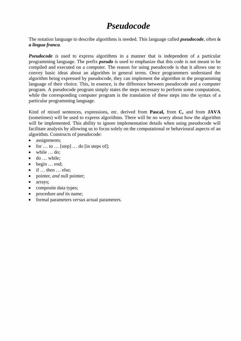
The content of stack after each operation will be: 7 8 8 8 56 3 5 5 13 13 13 13 69 69 72 9 9 9 9 9 9 9 9 9 9 648 nil The stack is useful also to verify the correctness of parentheses in an algebraic expression. If objects of stack fit to ordinary variables the straightforward implementation will look like expressed below. type link=^node; node=record key:integer; next:link; end; var head,z:link; procedure stackinit; begin new(head); new(z); head^.next:=z; z^.next:=z end; procedure push(v:integer); var t:link; begin new(t); t^.key:=v; t^.next:=head^.next; head^.next:=t end; function pop:integer; var t:link; begin t:=head^.next; pop:=t^.key; head^.next:=t^.next; dispose(t) end; function stackempty:boolean; begin stackempty:=(head^.next=z) end.

Implementation by the built-in data type of array: const maxP=100; var stack: array[0..maxP]of integer; p:integer; procedure push(v:integer); begin stack[p]:=v; p:=p+1 end; function pop:integer; begin p:=p-1; pop:=stack[p] end; procedure stackinit; begin p:=0 end; function stackempty:boolean; begin stackempty:=(p=<0) end.

The algebraic expression is implemented by using stack: stackinit; repeat repeat read(c) until c<>''; if c=')' then write(chr(pop)); if c='+' then push(ord(c)); if c='*' then push(ord(c)); while (c=>'0') and (c=<'9') do begin write(c); read(c) end; if c<>'(' then write(''); until eoln;

The QUEUE ADT This ADT covers a set of objects as well as operations performed on objects: • queueinit (Q) – creates a necessary structured space in computer memory to locate objects in

Q; • put (x) – inserts x into Q; • get – deletes object from the queue that has been residing in Q the longest; • head – returns an object from the queue that has been residing in Q the longest; • kill (Q) – releases an amount of memory occupied by Q. The operations with queue obey FIFO property: First-In-First-Out. This is a logical constrain or logical condition. The queue is a dynamic data set with a limited access to objects. The application to illustrate usage of a queue is:

queueing system simulation (system with waiting lines) (implemented by using the built-in type of pointer)

type link=^node; node=record key:integer; next:link; end; var head,tail,z:link; procedure queueinit; begin new(head); new(z); head^.next:=z; tail^.next=z; z^.next:=z end; procedure put(v:integer); var t:link; begin new(t); t^.key:=v; t^.next:=tail^.next; tail^.next:=t end; function get:integer; var t:link; begin t:=head^.next; get:=t^.key; head^.next:=t^.next; dispose(t)

end; function queueempty:boolean; begin queueempty:=(head^.next=z;tail^.next=z) end. The queue operations by array: const max=100; var queue:array[0..max] of integer; head,tail:integer; procedure put(v:integer); begin queue[tail]:=v; tail:=tail+1; if tail>max then tail:=0 end; function get: integer; begin get:=queue[head]; head:=head+1; if head>max then head:=0 end; procedure queueinitialize; begin head:=0; tail:=0 end; function queueempty:boolean; begin queueempty:=(head=tail) end.

The Queue Implementation A queue is used in computing in much the same way as it is used in everyday life: • to allow a sequence of items to be processed on a first-come-first-served basis. In most computer installations, for example, one printer is connected to several different machines, so that more than one user can submit printing jobs to the same printer. Since printing a job takes much longer than the process of actually transmitting the data from the computer to the printer, a queue of jobs is formed so that the jobs print out in the same order in which they were received by the printer. This has the irritating consequence that if your job consists of printing only a single page while the job in front of you is printing an entire 200-page thesis, you must still wait for the large job to finish before you can get your page. (All of which illustrates that Murphy's law applies equally well to the computer world as to the 'real' world, where, when you wish to buy one bottle of ketchup in a supermarket, you are stuck behind someone with a trolley containing enough to stock the average house for a month.) From the point of view of data structures, a queue is similar to a stack, in that data are stored in a linear fashion, and access to the data is allowed only at the ends of the queue. The actions allowed on a queue are: • Creating an empty queue. • Testing if a queue is empty. • Adding data to the tail of the queue. • Removing data from the head of the queue. These operations are similar to those for a stack, except that pushing has been replaced by adding an item to the tail of the queue, and popping has been replaced by removing an item from the head

of the queue. Because queues process data in the same order in which they are received, a queue is said to be a first-in-first out or FIFO data structure. Just as with stacks, queues can be implemented using arrays or lists. For the first of all, let’s consider the implementation using arrays. Define an array for storing the queue elements, and two markers: • one pointing to the location of the head of the queue, • the other to the first empty space following the tail. When an item is to be added to the queue, a test to see if the tail marker points to a valid location is made, then the item is added to the queue and the tail marker is incremented by 1. When an item is to be removed from the queue, a test is made to see if the queue is empty and, if not, the item at the location pointed to by the head marker is retrieved and the head marker is incremented by 1. This procedure works well until the first time when the tail marker reaches the end of the array. If some removals have occurred during this time, there will be empty space at the beginning of the array. However, because the tail marker points to the end of the array, the queue is thought to be 'full' and no more data can be added. We could shift the data so that the head of the queue returns to the beginning of the array each time this happens, but shifting data is costly in terms of computer time, especially if the data being

stored in the array consist of large data objects. A more efficient way of storing a queue in an array is to “wrap around” the end of the array so that it joins the front of the array. Such a cfrcular array allows the entire array (well, almost, as we'll see in a bit) to be used for storing queue elements without ever requiring any data to be shifted. A circular array with QSIZE elements (numbered from 0 to QSIZE-1) may be visualized: The array is, of course, stored in the normal way in memory, as a linear block of QSIZE elements. The circular diagram is just a convenient way of representing the data structure. We will need Head and Tail markers to indicate the location of the head and the location just after the tail where the next item should be added to the queue, respectively. An empty queue is denoted by the condition Head = Tail:

At this point, the first item of data would be added at the location indicated by the Tail marker, that is, at array index 0. Adding this element gives us the situation:

Let us use the queue until the Tail marker reaches QSIZE-1. We will assume that some items have been removed from the queue, so that Head has moved along as well:

Now we add another element to the queue at the location marked by Tail, that is, at array index QSIZE-1. The Tail marker now advances one step, which positions it at array index 0. The Tail marker has wrapped around the array and come back to its starting point. Since the Head marker has moved along, those elements at the beginning of the array from index 0 up to index Head-1 are available for storage. Using a circular array means that we can make use of these elements without having to shift any data. In a similar way, if we keep removing items from the queue, eventually Head will point to array index QSIZE-1. If we remove another element, Head will advance another step and wrap around the array, returning to index 0. We have seen that the condition for an empty queue is that Head == Tail. What is the condition for a full queue? If we try to make use of all the array elements, then in a full queue, the tail of the queue must be the element immediately prior to the head. Since we are using the Tail marker to point to the array element immediately following the tail element in the queue, Tail would have to point to the same location as Head for a full queue. But we have just seen that the condition Head == Tail is the condition for an empty queue. Therefore, if we try to make use of all the array elements, the conditions for full and empty queues become identical. We therefore impose the rule that we must always keep at least one free space in the array, and that a queue becomes full when the Tail marker points to the location immediately prior to Head. We may now formalize the algorithms for dealing with queues in a circular array. • Creating an empty queue: Set Head = Tail = 0. • Testing if a queue is empty: is Head == Tail? • Testing if a queue is full: is (Tail + 1) mod QSIZE == Head? • Adding an item to a queue: if queue is not full, add item at location Tail and set Tail = (Tail +

1) mod QSIZE. • Removing an item from a queue: if queue is not empty, remove item from location Head and

set Head = (Head + 1) mod QSIZE. The mod operator ensures that Head and Tail wrap around the end of the array properly.

For example, suppose that Tail is QSIZE-1 and we wish to add an item to the queue. We add the item at location Tail (assuming that the queue is not full) and then Set Tail

((QSIZE - 1) + 1) mod QSIZE = QSIZE mod QSIZE = 0

The List ADT A list is one of the most fundamental data structures used to store a collection of data items. The importance of the List ADT is that it can be used to implement a wide variety of other ADTs. That is, the LIST ADT often serves as a basic building block in the construction of more complicated ADTs. A list may be defined as a dynamic ordered n-tuple:

L == (l1, 12, ….., ln) The use of the term dynamic in this definition is meant to emphasize that the elements in this n-tuple may change over time. Notice that these elements have a linear order that is based upon their position in the list. The first element in the list, 11, is called the head of the list. The last element, ln, is referred to as the tail of the list. The number of elements in a list L is refered to as the length of the list. Thus the empty list, represented by (), has length 0. A list can homogeneous or heterogeneous. In many applications it is also useful to work with lists of lists. In this case, each element of the list is itself a list. For example, consider the list

((3), (4, 2, 5), (12, (8, 4)), ()) The operations we will define for accessing list elements are given below. For each of these operations, L represents a specific list. It is also assumed that a list has a current position variable that refers to some element in the list. This variable can be used to iterate through the elements of a list. 0. Initialize ( L ). This operation is needed to allocate the amount of memory and to give a

structure to this amount. 1. Insert (L, x, i). If this operation is successful, the boolean value true is returned; otherwise, the boolean value false is returned. 2. Append (L, x). Adds element x to the tail of L, causing the length of the list to become n+1. If this operation is successful, the boolean value true is returned; otherwise, the boolean value false is returned.

3. Retrieve (L, i). Returns the element stored at position i of L, or the null value if position i does

not exist. 4. Delete (L, i). Deletes the element stored at position i of L, causing elements to move in their positions. 5. Length (L). Returns the length of L. 6. Reset (L). Resets the current position in L to the head (i.e., to position 1) and returns the value 1. If the list is,empty, the value 0 is returned. 7. Current (L). Returns the current position in L. 8. Next (L). Increments and returns the current position in L. Note that only the Insert, Delete, Reset, and Next operations modify the lists to which they are applied. The remaining operations simply query lists in order to obtain information about them.

Sequential Mapping If all of the elements that comprise a given data structure are stored one after the other in consecutive memory locations, we say that the data structure is sequentially mapped into computer memory. Sequential mapping makes it possible to access any element in the data structure in constant time. Given the starting address of the data structure in memory, we can find the address of any element in the data structure by simply calculating its offset from the starting address. An array is an example of a sequentially mapped data structure:

Because it takes the same amount of time to access any element, a sequentially-mapped data structure is also called a random access data structure. That is, the accessing time is independent of the size of the data structure, and therefore requires O(l) time.

Schematic representations of (a) a singly-linked list and (b) a doubly-linked list:

List Operations Insert and Delete with Single-linked List and Double-linked List:

The Skip Lists:

The DYNAMIC SET ADT The set is a fundamental structure in mathematics. Compuer science view to a set: • it groups objects together; • the objects in a set are called the elements or members of the set; • these elements are taken from the universal set U, which contains all possible set elements; • all the members of- a given set are unique. The number of elements contained in a set S is referred to as the cardinality of S, denoted by |S|. It is often refered to a set with cardinality n as an n-set. The elements of a set are not ordered. Thus, {1, 2, 3} and {3, 2, 1} represent the same set. Mathematical operations with sets: • an element x is (or is not) a member of the set S; • the empty set; • two sets A and B are equal (or not); • an A is said to be a subset of B (the empty set is a subset of every set); • the union of A and B; • the intersection of A and B; • the difference of A and B; • the Cartesian product of two sets. In computer science it is often useful to consider set-like structures in which the ordering of the elements is important, such sets will be refered as an ordered n-tuple, like (al, a2, … an). The concept of a set serves as the basis for a wide variety of useful abstract data types. A large number of computer applications involve the manipulation of sets of data elements. Thus, it makes sense to investigate data structures and algorithms that support efficient implementation of various operations on sets. Another important difference between the mathematical concept of a set and the sets considered in computer science: • a set in mathematics is unchanging, while the sets in CS are considered to change over time as

data elements are added or deleted. Thus, sets are refered here as dynamic sets. In addition, we will assume that each element in a dynamic set contains an identifying field called a key, and that a total ordering relationship exists on these keys. It will be assumed that no two elements of a dynamic set contain the same key. The concept of a dynamic set as an DYNAMIC SET ADT is to be specified, that is, as a collection of data elements, along with the legal operations defined on these data elements. If the DYNAMIC SFT ADT is implemented properly, application programmers will be able to use dynamic sets without having to understand their implementation details. The use of ADTs in this manner simplifies design and development, and promotes reusability of software components.

A list of general operations for the DYNAMIC SET ADT. In each of these operations, S represents a specific dynamic set: 1. Search(S, k). Returns the element with key k in S, or the null value if an element with key k is

not in S. 2. Insert(S, x). Adds element x to S. If this operation is successful, the boolean value true is

returned; otherwise, the boolean value false is returned. 3. Delete(S, k). Removes the element with key k in S. If this operation is successful, the boolean

value true is returned; otherwise, the boolean value false is returned. 4. Minimum(S). Returns the element in dynamic set S that has the smallest key value, or the null

value if S is empty. 5. Maximum(S). Returns the element in S that has the largest key value, or the null value if S is

empty. 6. Predecessor(S, k). Returns the element in S that has the largest key value less than k, or the

null value if no such element exists. 7. Successor(S, k). Returns the element in S that has the smallest key value greater than k, or the

null value if no such element exists. In addition, when considering the DYNAMIC SET ADT (or any modifications of this ADT) we will assume the following operations are available: 1. Empty(S). Returns a boolean value, with true indicating that S is an empty dynamic set, and false indicating that S is not. 2. MakeEmpty(S). Clears S of all elements, causing S to become an empty dynamic set. Since these last two operations are often trivial to implement, they generally are to be omitted. In many instances an application will only require the use of a few DYNAMIC SET operations. Some groups of these operations are used so frequently that they are given special names: the ADT that supports Search, Insert, and Delete operations is called the DICTIONARY ADT; the STACK, QUEUE, and PRIORITY QUEUE ADTs are all special types of dynamic sets. A variety of data structures will be described in forthcoming considerations that they can be used to implement either the DYNAMIC SET ADT, or ADTs that support specific subsets of the DYNAMIC SET ADT operations. Each of the data structures described will be analyzed in order to determine how efficiently they support the implementation of these operations. In each case, the analysis will be performed in terms of n, the number of data elements stored in the dynamic set. This analysis will demonstrate that there is no optimal data structure for implementing dynamic sets. Rather, the best implementation choice will depend upon: • which operations need to be supported, • the frequency with which specific operations are used, • and possibly many other factors. As always, the more we know about how a specific application will use data, the better we can fine tune the associated data structures so that this data can be accessed efficiently.

Generalized Queues Specifically, pushdown stacks and FIFO queues are special instances of a more general

ADT: the generalized queue. Instances generalized queues differ in only the rule used when items are removed:

• for stacks, the rule is "remove the item that was most recently inserted";

• for FIFO queues, the rule is "remove the item that was least recently inserted";

• there are many other possibilities to consider.

A powerful alternative is the random queue, which uses the rule:

• "remove a random item"

The algorithm can expect to get any of the items on the queue with equal probability. The operations of a random queue can be implemented:

• in constant time using an array representation (it requires to reserve space ahead of time)

• using linked-list alternative (which is less attractive however, because implementing both insertion and deletion efficiently is a challenging task).

Random queues can be used as the basis for randomized algorithms, to avoid, with high probability, worst-case performance scenarios.

Stacks and FIFO queues are identifying items according to the time that they were inserted into the queue. Alternatively, the abstract concepts may be identified in terms of a sequential listing of the items in order, and refer to the basic operations of inserting and deleting items from the beginning and the end of the list:

• if we insert at the end and delete at the end, we get a stack (precisely as in array implementation);

• if we insert at the beginning and delete at the beginning, we also get a stack (precisely as in linked-list implementation);

• if we insert at the end and delete at the beginning, we get a FIFO queue (precisely as in linked-list implementation);

• if we insert at the beginning and delete at the end, we also get a FIFO queue (this option does not correspond to any of implementations given).

Building on this point of view, the deque ADT may be defined, where either insertion or deletion at either end are allowed. The implementation of deque is a good exercise to program.

The priority queue ADT is another example of generalized queue. The items in a priority queue have keys and the rule for deletion is:

"remove the item with the smallest key"

The priority queue ADT is useful in a variety of applications, and the problem of finding efficient implementations for this ADT has been a research goal in computer science for many years. Identifying and using the ADT in applications has been an important factor in this research:

• an immediate indication can be given for whether or not a new algorithm is correct by substituting its implementation for an old implementation in a huge, complex application and checking if there has been got the same result;

• an immediate indication can be given for whether a new algorithm is more efficient than an old one by noting the extent to which substituting the new implementation improves the overall running time (the data structures and algorithms for solving this problem will be considered later, they are interesting, ingenious, and effective).

The symbol tables ADT is one more example of generalized queues, where the items have keys and the rule for deletion is:

"remove an item whose key is equal to a given key, if there is one"

This ADT is perhaps the most important one to consider, and dozens of implementations will be examined.

Each of these ADTs also give rise to a number of related, but different, ADTs that suggest themselves as an outgrowth of careful examination of application programs and the performance of implementations.

Duplicate and Index Items

For many applications, the abstract items to be processed are unique, a quality that lead to modification of idea how stacks, FIFO queues, and other generalized ADTs should operate. Specifically, in this section, the effect of changing the specifications of stacks, FIFO queues, and generalized queues to disallow duplicate items in the data structure will be considered.

For example, a company that maintains a mailing list of customers might want to try to grow the list by performing insert operations from other lists gathered from many sources, but would not want the list to grow for an insert operation that refers to a customer already on the list. The same principle applies in a variety of other applications. For another example, consider the problem of routing a message through a complex communications network. It might be trials to go through several paths simultaneously in the network, but there is only one message. So any particular node in the network would want to have only one copy in its internal data structures.

One approach to handle this situation is to leave up to the programs the task of ensuring that duplicate items are not presented to the ADT. But since the purpose of an ADT is to provide clients with clean solution to application problems, the detection and resolution of duplicates have to be a part of ADT.

Disallowing duplicate items is a change in the abstraction:

• the interface, names of operations, and so forth for such an ADT are the same as those for the corresponding original ADT, but the behavior of the implementation changes in a fundamental way.

In general, modification of the specification of a structure gives a completely new ADT – one that has completely different properties. This situation also demonstrates the precarious nature of ADT specification:

• being sure that clients and implementations adhere to the specifications in an interface is difficult enough, but enforcing a high-level statement such as this one is another matter entirely.

In general, a generic decision has to be made when a client makes an insert request for an item that is already in the data structure:

• should it be proceeded as though the request never happened?

• or should it be proceeded as though the client had performed a delete followed by an insert?

This decision affects the order in which items are ultimately processed for ADTs such as stacks and FIFO queues, and the distinction is significant for programs. For example, the company using such an ADT for a mailing list might prefer to use the new item (perhaps assuming that it has more up-to-date information about the customer), and the switching mechanism using such an ADT might prefer to ignore the new item (perhaps it has already taken steps to send along the message).

Furthermore, such choice affects the implementations:

• the forget-the-old-item statement is generally more difficult to implement than the ignore-the-new-item statement, because it requires to modify the data structure.

To implement generalized queues with no duplicate items:

• an abstract operation for testing item equality has to be presented;

• the determination whether a new item to be inserted is already in the data structure has to be available.

There is an important special case with a straightforward solution:

• if the items are integers in the range [0, …, N-1], then a second array of size N, indexed by the item itself, to determine whether that item is in the stack, may be used.

Inserting the item, the ith entry in the second array may be set to 1; and deleting item i, the ith entry in the array may be set to 0. The same code as before may be used to insert and delete items, with one additional test:

the test to see whether the item is already in the structure.

If it is, the insert or delete operation have to be ignored. This solution does not depend on whether an array or linked-list (or some other) representation for the ADT. Implementing an ignore-the-old-item case involves more work.

In summary, one way to implement a generalized queue ADT with no duplicates using an ignore-the-new-item case is to maintain two data structures: the first contains the items in the structure, as before, to keep track of the order in which the items in the queue were inserted; the second is an array that allows us to keep track of which items are in the queue, by using the item as an index. Using an array in this way is a special case of a symbol-table implementation, which is discussed later.

This special case arises frequently. The most important example is when the items in the data structure are array indices themselves, so such items are referred as index items. Typically, a set of N objects, kept in yet another array, has to be passed through a generalized queue structure as a part of a more complex algorithm. Objects are put on the queue by index and processed when they are removed, and each object is to be processed precisely once. Using array indices in a queue with no duplicates accomplishes this goal directly.

Each of these choices (disallow duplicates, or do not; and use the new item, or do not) leads to a new ADT The differences may seem minor, but they obviously affect the dynamic behavior of the ADT as seen by programs, and affect the choice of algorithm and data structure to implement the various operations, so there is no alternative but to treat all the ADTs as different.

Furthermore, in many cases additional options have to be considered. For example, there might be the wish to modify the interface to inform the client program when it attempts to insert a duplicate item, or to give the client the option whether to ignore the new item or to forget the old one.

To conclude, informally using a term such as pushdown stack, FIFO queue, deque, priority queue, or symbol table, it potentially referees to a family of ADTs, each with different sets of defined operations and different sets of conventions about the meanings of the operations, each requiring different and, in some cases, more sophisticated implementations to be able to support those operations efficiently.

First class ADT The objects of built-in data types and in ADTs considered above are disarmingly simple, there

is only one object in a given program and no possibility to declare variables of different types in client programs for the same ADT.

A first-class data type is one for which there is potentially many different instances, and which can be assigned to variables declared to hold the instances.

For example, it could be used first-class data types as arguments and return values to functions.

The implemention of first-class data types have to provide us with the capability to write programs that manipulate stacks and FIFO queues in much the same way as with types of data in programming language like C. This capability is important in the study of algorithms because it gives a natural way to express high level operations involving such ADTs. For example, two queues can be joined into one.

Some modern languages provide specific mechanisms for building first-class ADTs. Being able to manipulate instances of ADTs in much the same way that of built-in data types int or float, it allows any application program to be written such that the program manipulates the objects of central concern to the application; it allows many programmers to work simultaneously on large systems, all using a precisely defined set of abstract operations, and it provides for those abstract operations to be implemented in many different ways without any changes to the applications code - for example for new machines and programming environments. Some languages even allow operator overloading, to use basic symbols such as + or * to define operators.

First-class ADTs play a central role in many of implementations because they provide the necessary support for the abstract mechanisms for generic objects and collections of objects.

Nevertheless, the ability to have multiple instances of a given ADT in a single program can lead to complicated situations:

• Do we want to be able to have stacks or queues with different types of objects on them?

• How about different types of objects on the same queue?

• Do we want to use different implementations for queues of the same type in a single client because we know of performance differences?

• Should information about the efficiency of implementations be included in the interface?

• What form should that information take?

Such questions underscore the importance of understanding the basic characteristics of algorithms and data structures and how client programs may use them effectively.

Heaps, Heapsort and Priority Queues The application of a purely binary tree is a data structure called a heap. Heaps are unusual in the menagerie of tree structures in that they represent trees as arrays (rather than linked structures using pointers). Level-ordering of the tree may be expressed:

Numbering of a tree’s nodes for storage in a array If we use the number of a node as an array Index, this technique gives us an order in which we can store tree nodes in an array. The tree may be easily reconstructed from the array:

the left child of node number k has index 2k and the right child has index 2k + 1.

1 2 3 4 5 6 7 8 9 10 11 12 13 14 15 1 2 3 4 5 6 7 8 9 10 11 12 13 14 15 Any binary tree can be represented in an array in this fashion. This is not an efficient way to store just any binary tree, there would be many array elements that are left empty. A heap, however, is a special kind of binary tree that leaves no gaps in an array implementation:

• All leaves are on two adjacent levels. • All leaves on the lowest level occur at the left of the tree. • All levels above the lowest are completely filled. • Both children of any node are again heaps. • The value stored at any node is at least as large as the values in its two children.

The first three conditions ensure that the array representation of the heap will have no gaps in it. The last two conditions give a heap a weak amount of order. The order in which the elements are stored in the array will, in general, not be a sorted representation of the list, although the largest element will be stored at location 1.

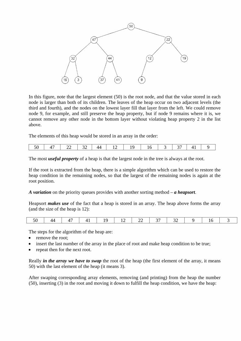
In this figure, note that the largest element (50) is the root node, and that the value stored in each node is larger than both of its children. The leaves of the heap occur on two adjacent levels (the third and fourth), and the nodes on the lowest layer fill that layer from the left. We could remove node 9, for example, and still preserve the heap property, but if node 9 remains where it is, we cannot remove any other node in the bottom layer without violating heap property 2 in the list above. The elements of this heap would be stored in an array in the order:

50 47 22 32 44 12 19 16 3 37 41 9 The most useful property of a heap is that the largest node in the tree is always at the root. If the root is extracted from the heap, there is a simple algorithm which can be used to restore the heap condition in the remaining nodes, so that the largest of the remaining nodes is again at the root position. A variation on the priority queues provides with another sorting method – a heapsort. Heapsort makes use of the fact that a heap is stored in an array. The heap above forms the array (and the size of the heap is 12):

50 44 47 41 19 12 22 37 32 9 16 3 The steps for the algorithm of the heap are: • remove the root; • insert the last number of the array in the place of root and make heap condition to be true; • repeat then for the next root. Really in the array we have to swap the root of the heap (the first element of the array, it means 50) with the last element of the heap (it means 3). After swaping corresponding array elements, removing (and printing) from the heap the number (50), inserting (3) in the root and moving it down to fulfill the heap condition, we have the heap:

'I'he contents of the array are now (and the heap size is 11):

47 44 22 41 19 12 3 37 32 9 16 50 If we repeat the process with a new root (47), we obtain the heap shown:

'I'he last two numbers in the array are no longer part of the heap, and contain the two largest numbers in sorted order. The array elements are now (with a heap size of 10):

44 41 22 37 19 12 3 16 32 9 47 50 The process continues in the same manner until the heap size has been reduced to zero, at which point the array contains the numbers in sorted order. If a heap is used purely for sorting, the heapsort algorithm turns out to be an O(n log n) algorithm. Although the heapsort is only about half as efficient as quicksort or mergesort for randomly ordered initial lists. The same technique can be used to implement a priority queue. Rather than carry the sorting process through to the bitter end, the root node can be extracted (which is the item with highest priority) and rearrange the tree, so that the remaining nodes form a heap with one less element. We need not process the data any further until the next request comes in for an item from the priority queue.

A heap is an efficient way of implementing a priority queue since the maximum number of nodes that need to be considered to restore the heap property when the root is extracted is about twice the depth of the tree. The number of comparisons is around 2 log N A priority queue is an ordinary queue, except that each item in the queue has an associated priority. Items with higher priority will get processed before items with lower priority, even if they arrive in the queue after them.

Priority Queues In many applications, records with keys must be processed in order, but not necessarily in full sorted order and not necessarily all at once. Often a set of records must be collected, then the largest processed, then perhaps more records collected, then the next largest processed, and so forth. An appropriate data structure in such an environment is one which supports the operations of inserting a new element and deleting the largest element. Such a data structure, which can be contrasted with queues (delete the oldest) and stacks (delete the newest) is called a priority queue. In fact, the priority queue might be thought of as a generalization of the stack and the queue (and other simple data structures), since these data structures can be implemented with priority queues, using appropriate priority assignments. Applications of priority queues include simulation systems (where the keys might correspond to "event times" which must be processed in order), job scheduling in computer systems (where the keys might correspond to "priorities" indicating which users should be processed first), and numerical computations (where the keys might be computational errors, so the largest can be worked on first). It is useful to be somewhat more precise about how to manipulate a priority queue, since there are several operations we may need to perform on priority queues in order to maintain them and use them effectively for applications such as those mentioned above. Indeed, the main reason that priority queues are so useful is their flexibility in allowing a variety of different operations to be efficiently performed on sets of records with keys. We want to build and maintain a data structure containing records with numerical keys (priorities) and supporting some of the following operations:

Construct a priority queue from N given items. Insert a new item. Remove the largest item. Replace the largest item with a new item (unless the new item is larger). Change the priority of an item. Delete an arbitrary specified item. Join two priority queues into one large one.

(If records can have duplicate keys, we take "largest" to mean "any record with the largest key value.") Different implementations of priority queues involve different performance characteristics for the various operations to be performed, leading to cost tradeoffs. Indeed, performance differences are really the only differences that can arise in the abstract data structure concept. First, we'll illustrate this point by discussing a few elementary data structures for implementing priority queues. Next, we'll examine a more advanced data structure and then show how the

various operations can be implemented efficiently using this data structure. We'll then look at an important sorting algorithm that follows naturally from these implementations. Any priority queue algorithm can be turned into a sorting algorithm by repeatedly using insert to build a priority queue containing all the items to be sorted, then repeatedly using remove to empty the priority queue, receiving the items in reverse order. Using a priority queue represented as an unordered list in this way corresponds to selection sort; using the ordered list corresponds to insertion sort. Although heaps are fairly sloppy in keeping their members in strict order, they are very good at rinding the maximum member and bringing it to the top of the heap.

Algorithms on Heaps The priority queue algorithms on heaps all work by first making a simple structural modification which could violate the heap condition, then traveling through the heap modifying it to ensure that the heap condition is satisfied everywhere. Some of the algorithms travel through the heap from bottom to top, others from top to bottom. In all of the algorithms,,we'll assume that the records are one-word integer keys stored in an array a of some maximum size, with the current size of the heap kept in an integer N. Note that N is as much a part of the definition of the heap as the keys and records themselves. To be able to build a heap, it is necessary first to implement the insert operation. Since this operation will increase the size of the heap by one, N must be incremented. Then the record to be inserted is put into a [N], but this may violate the heap property. If the heap property is violated (the new node is greater than its parent), then the violation can be fixed by exchanging the new node with its parent. This may, in turn, cause a violation, and thus can be fixed in the same way. For example, if P is to be inserted in the heap above, it is first stored in a [N] as the right child of M. Then, since it is greater than M, it is exchanged with M, and since it is greater than 0, it is exchanged with 0, and the process terminates since it is less that X. The heap shown in figure below results.

Inserting a new element (P) into a heap.

The code for this method is straightforward. In the following implementation, insert adds a new item to a [N], then calls upheap (N) to fix the heap condition violation at N:

procedure upheap(k: integer); var v: integer; begin v:=a[k]; a[O]:=maxint; while a [k div 2 1 < =v do begin a [k ]:=a [k div 2 1; k:=k div 2 end; a [k ]:=v

end; procedure insert(v: integer);

begin N:=N+l; a[N]:=v; upheap (N) end;

If k div 2 were replaced by k-1 everywhere in this program, we would have in essence one step of insertion sort (implementing a priority queue with an ordered list); here, instead, we are "inserting" the new key along the path from N to the root. As with insertion sort, it is not necessary to do a full exchange within the loop, because v is always involved in the exchanges. The replace operation involves replacing the key at the root with a new key, then moving down the heap from top to bottom to restore the heap condition. For example, if the X in the heap above is to be replaced with C, the first step is to store C at the root. This violates the heap condition, but the violation can be fixed by exchanging C with T, the larger of the two children of the root. This creates a violation at the next level, which can again be fixed by exchanging C with the larger of its two children (in this case S). The process continues until the heap condition is no longer violated at the node occupied by C. In the example, C makes it all the way to the bottom of the heap, leaving the heap depicted in figure next:

Replacing the largest key in a heap (with C)

The "remove the largest" operation involves almost the same process. Since the heap will be one element smaller after the operation, it is necessary to decrement N, leaving no place for the element that was stored in the last position. But the largest element (which is in a [ 1 ]) is to be removed, so the remove operation amounts to a replace, using the element that was in a [N]. The heap shown in figure is the result of removing the T from the heap in figure preceeding by replacing it with the M, then moving down, promoting the larger of the two children, until reaching a node with both children smaller than M. The implementation of both of these operations is centered around the process of fixing up a heap which satisfies the heap condition everywhere except possibly at the root. If the key at the root is too small, it must be moved down the heap without violating the heap property at any of the nodes touched. It turns out that the same operation can be used to fix up the heap after the value in any position is lowered. It may be implemented as follows:

label 0; var i.i. v: integer; begin v:=a [k while k<=N div 2 do

begin j:=k+k; if j<N then if a Ul <a U+l if v > =a U ] then goto 0; a[kl:=aU]; k:=j; end;

0: a[k]:=v end;

procedure downheap(k: integer); label 0; var i,j. v: integer; begin v: =a [k 1;

while k<=N div 2 do begin j:=k+k; if j<N then if a Ul <a U+l I then j:=j+l; if v >=a [ j ] then goto 0; a[kl:=aU]; k:=j;

end; 0: a[k]:=v

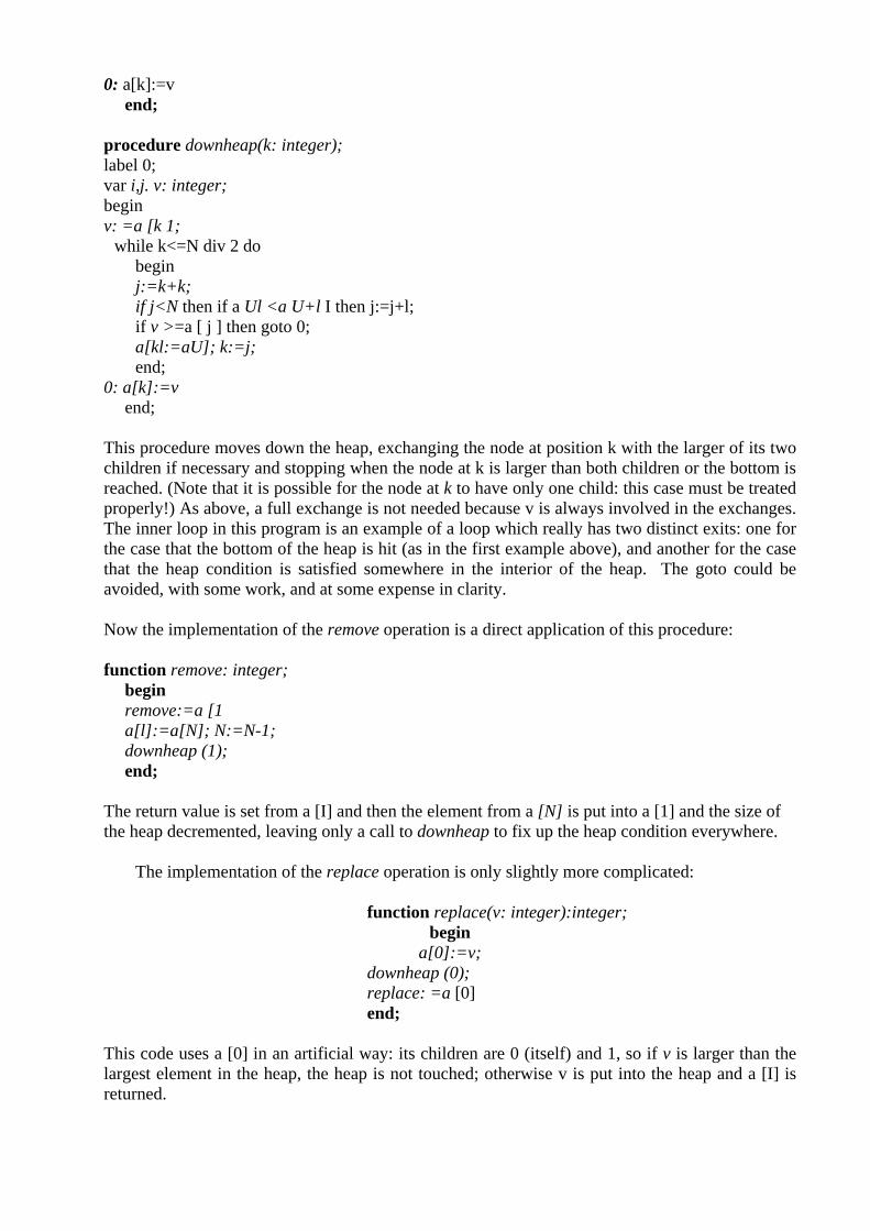
end; This procedure moves down the heap, exchanging the node at position k with the larger of its two children if necessary and stopping when the node at k is larger than both children or the bottom is reached. (Note that it is possible for the node at k to have only one child: this case must be treated properly!) As above, a full exchange is not needed because v is always involved in the exchanges. The inner loop in this program is an example of a loop which really has two distinct exits: one for the case that the bottom of the heap is hit (as in the first example above), and another for the case that the heap condition is satisfied somewhere in the interior of the heap. The goto could be avoided, with some work, and at some expense in clarity. Now the implementation of the remove operation is a direct application of this procedure: function remove: integer;

begin remove:=a [1 a[l]:=a[N]; N:=N-1; downheap (1); end;

The return value is set from a [I] and then the element from a [N] is put into a [1] and the size of the heap decremented, leaving only a call to downheap to fix up the heap condition everywhere.

The implementation of the replace operation is only slightly more complicated:

function replace(v: integer):integer; begin

a[0]:=v; downheap (0); replace: =a [0] end;

This code uses a [0] in an artificial way: its children are 0 (itself) and 1, so if v is larger than the largest element in the heap, the heap is not touched; otherwise v is put into the heap and a [I] is returned.

The delete operation for an arbitrary element from the heap and the change operation can also be implemented by using a simple combination of the methods above. For example, if the priority of the element at position k is raised, then upheap(k) can be called, and if it is lowered then downheap(k) does the job. Property 1 All of the basic operations insert, remove, replace, (downheap and upheap), delete, and change require less than 2 Ig N comparisons when performed on a heap of N elements. All these operations involve moving along a path between the root and the bottom of the heap, which includes no more than IgN elements for a heap of size N. The factor of two comes from downheap, which makes two comparisons in its inner loop; the other operations require only IgN comparisons. Note carefully that thejoin operation is not included on this list. Doing this operation efficiently seems to require a much more sophisticated data structure. On the other hand, in many applications, one would expect this operation to be required much less frequently than the others.

Indirect Heaps For many applications of priority queues, we don't want the records moved around at all. Instead, we want the priority queue routine not to return values but to tell us which of the records is the largest, etc. This is akin to the "indirect sort" or the "pointer sort". Modifying the above programs to work in this way is straightforward, though sometimes confusing. It will be worthwhile to examine this in more detail here because it is so convenient to use heaps in this way. Instead of rearranging the keys in the array a the priority queue routines will work with an array p of indices into the array a, such that a [p [k ] ] is the record corresponding to the kth element of the heap, for k between I and N. Moreover, we want to maintain another array q which keeps the heap position of the kth array element. This is the mechanism that we use to allow the (-hange and delete operations. Thus the q entry for the largest element in the array is 1, and so on.

We start with p [k ]=q [k I=k for k from I to N, which indicates that no rearrangement has been done. The code for heap construction looks much the same as before:

procedure pqconstruct; var k: integer; begin N:=M; for k:=l to N do

begin p [k ]:=k; q [k ]:=k end; for k: =M div 2 downto 1 do pqdownheap (k); end;

(We'll prefix implementations of priority-queue routines based on indirect heaps with "pq" for identification when they are used in later chapters.)

Indirectheap data structures

Now, to modify downheap to work indirectly, we need only examine the places where it

references a. Where it did a (-omparison before, it must now access a indirectly through p. Where it did a move before, it must now make the move in p, not a, and it must modify q accordingly. This leads to the following implementation:

procedure pqdownheap (k: integer); label 0; var j, v: integer; begin v:=p [k while k<= N div 2 do

begin j:=k+k;

if j<N then if a [p Ul I <a [p [j+1]] then j:=j+l; if a[v]>=a[p[j]] then goto 0; p[k]:=pU]; q[pU]]:=k; k:=j; end;

0: p [k ]:=v; q [v ]:=k end; The other procedures given above can be modified in a similar fashion to implement pqinsert," "pqchange," etc.

A similar indirect implementation can be developed based on maintaining p as an array of pointers to separately allocated records. In this case, a little more work is required to implement the function of q (find the heap position, given the record).

Advanced Implementations

If the join operation must be done efficiently, then the implementations that we have done so far are insufficient and more advanced techniques are needed. By "efficiently," we mean that a join should be done in about the same time as the other operations. This immediately rules out the linkless representation for heaps that we have been using, since two large heaps can be joined only by moving all the elements in at least one of them to a large array. It is easy to translate the algorithms we have been examining to use linked representations; in fact, sometimes there are other reasons for doing so (for example, it might be inconvenient to have a large contiguous array). In a direct linked representation, links would have to be kept in each node pointing to the parent and both children.

It turns out that the heap condition itself seems to be too strong to allow efficient

implementation of the join operation. The advanced data structures designed to solve this problem all weaken either the heap or the balance condition in order to gain the flexibility needed for the join. These structures allow all the operations to be completed in logarithmic time.