Data Structures and Algorithms

Course at D-MATH (CSE) of ETH Zurich

Felix Friedrich

FS 2019

1

1. Introduction

Overview, Algorithms and Data Structures, Correctness, FirstExample

19

Goals of the course

Understand the design and analysis of fundamental algorithmsand data structures.An advanced insight into a modern programming model (withC++).Knowledge about chances, problems and limits of the parallel andconcurrent computing.

20

Contentsdata structures / algorithmsThe notion invariant, cost model, Landau notation

algorithms design, inductionsearching, selection and sorting

amortized analysisdynamic programming

dictionaries: hashing and search treesFundamental algorithms on graphs,

shortest paths, Max-Flow

van-Emde Boas Trees, Splay-Trees

Minimum Spanning Trees, Fibonacci Heaps

prorgamming with C++RAII, Move Konstruktion, Smart Pointers,

Templates and generic programmingExceptions functors and lambdas

threads, mutex and monitorspromises and futures

parallel programmingparallelism vs. concurrency, speedup (Amdahl/-Gustavson), races, memory reordering, atomir reg-isters, RMW (CAS,TAS), deadlock/starvation

22

1.2 Algorithms

[Cormen et al, Kap. 1;Ottman/Widmayer, Kap. 1.1]

23

Algorithm

Algorithm: well defined computing procedure to compute output datafrom input data

24

example problem

Input: A sequence of n numbers (a1, a2, . . . , an)

Output: Permutation (a′1, a′2, . . . , a

′n) of the sequence (ai)1≤i≤n, such that

a′1 ≤ a′2 ≤ · · · ≤ a′n

Possible input(1, 7, 3), (15, 13, 12,−0.5), (1) . . .

Every example represents a problem instance

The performance (speed) of an algorithm usually depends on theproblem instance. Often there are “good” and “bad” instances.

25

example problem

Input: A sequence of n numbers (a1, a2, . . . , an)Output: Permutation (a′1, a

′2, . . . , a

′n) of the sequence (ai)1≤i≤n, such that

a′1 ≤ a′2 ≤ · · · ≤ a′n

Possible input(1, 7, 3), (15, 13, 12,−0.5), (1) . . .

Every example represents a problem instance

The performance (speed) of an algorithm usually depends on theproblem instance. Often there are “good” and “bad” instances.

25

example problem

Input: A sequence of n numbers (a1, a2, . . . , an)Output: Permutation (a′1, a

′2, . . . , a

′n) of the sequence (ai)1≤i≤n, such that

a′1 ≤ a′2 ≤ · · · ≤ a′n

Possible input(1, 7, 3), (15, 13, 12,−0.5), (1) . . .

Every example represents a problem instance

The performance (speed) of an algorithm usually depends on theproblem instance. Often there are “good” and “bad” instances.

25

example problem

Input: A sequence of n numbers (a1, a2, . . . , an)Output: Permutation (a′1, a

′2, . . . , a

′n) of the sequence (ai)1≤i≤n, such that

a′1 ≤ a′2 ≤ · · · ≤ a′n

Possible input(1, 7, 3), (15, 13, 12,−0.5), (1) . . .

Every example represents a problem instance

The performance (speed) of an algorithm usually depends on theproblem instance. Often there are “good” and “bad” instances.

25

Examples for algorithmic problems

Tables and statistis: sorting, selection and searching

routing: shortest path algorithm, heap data structureDNA matching: Dynamic Programmingevaluation order: Topological Sortingautocomletion and spell-checking: Dictionaries / TreesFast Lookup : Hash-TablesThe travelling Salesman: Dynamic Programming, MinimumSpanning Tree, Simulated Annealing

26

Examples for algorithmic problems

Tables and statistis: sorting, selection and searchingrouting: shortest path algorithm, heap data structure

DNA matching: Dynamic Programmingevaluation order: Topological Sortingautocomletion and spell-checking: Dictionaries / TreesFast Lookup : Hash-TablesThe travelling Salesman: Dynamic Programming, MinimumSpanning Tree, Simulated Annealing

26

Examples for algorithmic problems

Tables and statistis: sorting, selection and searchingrouting: shortest path algorithm, heap data structureDNA matching: Dynamic Programming

evaluation order: Topological Sortingautocomletion and spell-checking: Dictionaries / TreesFast Lookup : Hash-TablesThe travelling Salesman: Dynamic Programming, MinimumSpanning Tree, Simulated Annealing

26

Examples for algorithmic problems

Tables and statistis: sorting, selection and searchingrouting: shortest path algorithm, heap data structureDNA matching: Dynamic Programmingevaluation order: Topological Sorting

autocomletion and spell-checking: Dictionaries / TreesFast Lookup : Hash-TablesThe travelling Salesman: Dynamic Programming, MinimumSpanning Tree, Simulated Annealing

26

Examples for algorithmic problems

Tables and statistis: sorting, selection and searchingrouting: shortest path algorithm, heap data structureDNA matching: Dynamic Programmingevaluation order: Topological Sortingautocomletion and spell-checking: Dictionaries / Trees

Fast Lookup : Hash-TablesThe travelling Salesman: Dynamic Programming, MinimumSpanning Tree, Simulated Annealing

26

Examples for algorithmic problems

Tables and statistis: sorting, selection and searchingrouting: shortest path algorithm, heap data structureDNA matching: Dynamic Programmingevaluation order: Topological Sortingautocomletion and spell-checking: Dictionaries / TreesFast Lookup : Hash-Tables

The travelling Salesman: Dynamic Programming, MinimumSpanning Tree, Simulated Annealing

26

Examples for algorithmic problems

Tables and statistis: sorting, selection and searchingrouting: shortest path algorithm, heap data structureDNA matching: Dynamic Programmingevaluation order: Topological Sortingautocomletion and spell-checking: Dictionaries / TreesFast Lookup : Hash-TablesThe travelling Salesman: Dynamic Programming, MinimumSpanning Tree, Simulated Annealing

26

Characteristics

Extremely large number of potential solutionsPractical applicability

27

Data Structures

A data structure is a particular way oforganizing data in a computer so thatthey can be used efficiently (in thealgorithms operating on them).Programs = algorithms + datastructures.

28

Efficiency

Illusion:

If computers were infinitely fast and had an infinite amount ofmemory ...... then we would still need the theory of algorithms (only) forstatements about correctness (and termination).

Reality: resources are bounded and not free:

Computing time→ EfficiencyStorage space→ Efficiency

Actually, this course is nearly only about efficiency.

29

Efficiency

Illusion:

If computers were infinitely fast and had an infinite amount ofmemory ...... then we would still need the theory of algorithms (only) forstatements about correctness (and termination).

Reality: resources are bounded and not free:

Computing time→ EfficiencyStorage space→ Efficiency

Actually, this course is nearly only about efficiency.29

Hard problems.

NP-complete problems: no known efficient solution (the existenceof such a solution is very improbable – but it has not yet beenproven that there is none!)Example: travelling salesman problem

This course is mostly about problems that can be solvedefficiently (in polynomial time).

30

2. Efficiency of algorithms

Efficiency of Algorithms, Random Access Machine Model, FunctionGrowth, Asymptotics [Cormen et al, Kap. 2.2,3,4.2-4.4 |Ottman/Widmayer, Kap. 1.1]

31

Efficiency of Algorithms

Goals

Quantify the runtime behavior of an algorithm independent of themachine.Compare efficiency of algorithms.Understand dependece on the input size.

32

Programs and Algorithms

program

programming language

computer

algorithm

pseudo-code

computation model

implemented in

specified for

specified in

based on

Technology Abstraction

33

Technology Model

Random Access Machine (RAM)

Execution model: instructions are executed one after the other (onone processor core).

Memory model: constant access time (big array)Fundamental operations: computations (+,−,·,...) comparisons,assignment / copy on machine words (registers), flow control(jumps)Unit cost model: fundamental operations provide a cost of 1.Data types: fundamental types like size-limited integer or floatingpoint number.

34

Technology Model

Random Access Machine (RAM)

Execution model: instructions are executed one after the other (onone processor core).Memory model: constant access time (big array)

Fundamental operations: computations (+,−,·,...) comparisons,assignment / copy on machine words (registers), flow control(jumps)Unit cost model: fundamental operations provide a cost of 1.Data types: fundamental types like size-limited integer or floatingpoint number.

34

Technology Model

Random Access Machine (RAM)

Execution model: instructions are executed one after the other (onone processor core).Memory model: constant access time (big array)Fundamental operations: computations (+,−,·,...) comparisons,assignment / copy on machine words (registers), flow control(jumps)

Unit cost model: fundamental operations provide a cost of 1.Data types: fundamental types like size-limited integer or floatingpoint number.

34

Technology Model

Random Access Machine (RAM)

Execution model: instructions are executed one after the other (onone processor core).Memory model: constant access time (big array)Fundamental operations: computations (+,−,·,...) comparisons,assignment / copy on machine words (registers), flow control(jumps)Unit cost model: fundamental operations provide a cost of 1.

Data types: fundamental types like size-limited integer or floatingpoint number.

34

Technology Model

Random Access Machine (RAM)

Execution model: instructions are executed one after the other (onone processor core).Memory model: constant access time (big array)Fundamental operations: computations (+,−,·,...) comparisons,assignment / copy on machine words (registers), flow control(jumps)Unit cost model: fundamental operations provide a cost of 1.Data types: fundamental types like size-limited integer or floatingpoint number.

34

Size of the Input Data

Typical: number of input objects (of fundamental type).

Sometimes: number bits for a reasonable / cost-effectiverepresentation of the data.

fundamental types fit into word of size : w ≥ log(sizeof(mem)) bits.

35

Pointer Machine Model

We assume

Objects bounded in size can be dynamically allocated in constanttimeFields (with word-size) of the objects can be accessed in constanttime 1.

top xn xn−1 x1 null

36

Asymptotic behavior

An exact running time of an algorithm can normally not be predictedeven for small input data.

We consider the asymptotic behavior of the algorithm.And ignore all constant factors.

ExampleAn operation with cost 20 is no worse than one with cost 1Linear growth with gradient 5 is as good as linear growth withgradient 1.

37

2.2 Function growth

O, Θ, Ω [Cormen et al, Kap. 3; Ottman/Widmayer, Kap. 1.1]

39

Superficially

Use the asymptotic notation to specify the execution time ofalgorithms.

We write Θ(n2) and mean that the algorithm behaves for large n liken2: when the problem size is doubled, the execution time multipliesby four.

40

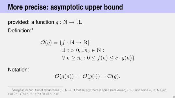
More precise: asymptotic upper bound

provided: a function g : N→ R.

Definition:1

O(g) = f : N→ R|∃ c > 0,∃n0 ∈ N :

∀ n ≥ n0 : 0 ≤ f(n) ≤ c · g(n)

Notation:O(g(n)) := O(g(·)) = O(g).

1Ausgesprochen: Set of all functions f : N→ R that satisfy: there is some (real valued) c > 0 and some n0 ∈ N suchthat 0 ≤ f(n) ≤ n · g(n) for all n ≥ n0.

41

Graphic

g(n) = n2

f ∈ O(g)

n0 n42

Graphic

g(n) = n2

f ∈ O(g)

h ∈ O(g)

n0

n42

Examples

O(g) = f : N→ R| ∃c > 0,∃n0 ∈ N : ∀n ≥ n0 : 0 ≤ f(n) ≤ c · g(n)

f(n) f ∈ O(?) Example3n+ 4

O(n) c = 4, n0 = 4

2n

O(n) c = 2, n0 = 0

n2 + 100n

O(n2) c = 2, n0 = 100

n+√n

O(n) c = 2, n0 = 1

43

Examples

O(g) = f : N→ R| ∃c > 0,∃n0 ∈ N : ∀n ≥ n0 : 0 ≤ f(n) ≤ c · g(n)

f(n) f ∈ O(?) Example3n+ 4 O(n) c = 4, n0 = 42n

O(n) c = 2, n0 = 0

n2 + 100n

O(n2) c = 2, n0 = 100

n+√n

O(n) c = 2, n0 = 1

43

Examples

O(g) = f : N→ R| ∃c > 0,∃n0 ∈ N : ∀n ≥ n0 : 0 ≤ f(n) ≤ c · g(n)

f(n) f ∈ O(?) Example3n+ 4 O(n) c = 4, n0 = 42n O(n) c = 2, n0 = 0n2 + 100n

O(n2) c = 2, n0 = 100

n+√n

O(n) c = 2, n0 = 1

43

Examples

O(g) = f : N→ R| ∃c > 0,∃n0 ∈ N : ∀n ≥ n0 : 0 ≤ f(n) ≤ c · g(n)

f(n) f ∈ O(?) Example3n+ 4 O(n) c = 4, n0 = 42n O(n) c = 2, n0 = 0n2 + 100n O(n2) c = 2, n0 = 100n+√n

O(n) c = 2, n0 = 1

43

Examples

O(g) = f : N→ R| ∃c > 0,∃n0 ∈ N : ∀n ≥ n0 : 0 ≤ f(n) ≤ c · g(n)

f(n) f ∈ O(?) Example3n+ 4 O(n) c = 4, n0 = 42n O(n) c = 2, n0 = 0n2 + 100n O(n2) c = 2, n0 = 100n+√n O(n) c = 2, n0 = 1

43

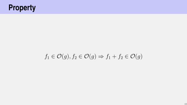
Property

f1 ∈ O(g), f2 ∈ O(g)⇒ f1 + f2 ∈ O(g)

44

Converse: asymptotic lower bound

Given: a function g : N→ R.

Definition:

Ω(g) = f : N→ R|∃ c > 0,∃n0 ∈ N :

∀ n ≥ n0 : 0 ≤ c · g(n) ≤ f(n)

45

Example

g(n) = n

f ∈ Ω(g)

n0 n

46

Example

g(n) = n

f ∈ Ω(g)h ∈ Ω(g)

n0 n

46

Asymptotic tight bound

Given: function g : N→ R.

Definition:

Θ(g) := Ω(g) ∩ O(g).

Simple, closed form: exercise.

47

Example

g(n) = n2

f ∈ Θ(n2)

h(n) = 0.5 · n2

n48

Notions of Growth

O(1) bounded array accessO(log log n) double logarithmic interpolated binary sorted sortO(log n) logarithmic binary sorted searchO(√n) like the square root naive prime number test

O(n) linear unsorted naive searchO(n log n) superlinear / loglinear good sorting algorithmsO(n2) quadratic simple sort algorithmsO(nc) polynomial matrix multiplyO(2n) exponential Travelling Salesman Dynamic ProgrammingO(n!) factorial Travelling Salesman naively

49

Small n

2 3 4 5 6

20

40

60

lnnn

n2

n42n

50

Larger n

5 10 15 20

0.2

0.4

0.6

0.8

1·106

log nnn2

n4

2n

51

“Large” n

20 40 60 80 100

0.2

0.4

0.6

0.8

1·1020

log nnn2n4

2n

52

Logarithms

10 20 30 40 50

200

400

600

800

1,000

n

n2

n3/2

log n

n log n

53

Time Consumption

Assumption 1 Operation = 1µs.

problem size 1 100 10000 106 109

log2 n 1µs

7µs 13µs 20µs 30µs

n 1µs

100µs 1/100s 1s 17 minutes

n log2 n 1µs

700µs 13/100µs 20s 8.5 hours

n2 1µs

1/100s 1.7 minutes 11.5 days 317 centuries

2n 1µs

1014 centuries ≈ ∞ ≈ ∞ ≈ ∞

54

Time Consumption

Assumption 1 Operation = 1µs.

problem size 1 100 10000 106 109

log2 n 1µs

7µs 13µs 20µs 30µs

n 1µs 100µs 1/100s 1s 17 minutes

n log2 n 1µs

700µs 13/100µs 20s 8.5 hours

n2 1µs

1/100s 1.7 minutes 11.5 days 317 centuries

2n 1µs

1014 centuries ≈ ∞ ≈ ∞ ≈ ∞

54

Time Consumption

Assumption 1 Operation = 1µs.

problem size 1 100 10000 106 109

log2 n 1µs

7µs 13µs 20µs 30µs

n 1µs 100µs 1/100s 1s 17 minutes

n log2 n 1µs

700µs 13/100µs 20s 8.5 hours

n2 1µs 1/100s 1.7 minutes 11.5 days 317 centuries

2n 1µs

1014 centuries ≈ ∞ ≈ ∞ ≈ ∞

54

Time Consumption

Assumption 1 Operation = 1µs.

problem size 1 100 10000 106 109

log2 n 1µs 7µs 13µs 20µs 30µs

n 1µs 100µs 1/100s 1s 17 minutes

n log2 n 1µs

700µs 13/100µs 20s 8.5 hours

n2 1µs 1/100s 1.7 minutes 11.5 days 317 centuries

2n 1µs

1014 centuries ≈ ∞ ≈ ∞ ≈ ∞

54

Time Consumption

Assumption 1 Operation = 1µs.

problem size 1 100 10000 106 109

log2 n 1µs 7µs 13µs 20µs 30µs

n 1µs 100µs 1/100s 1s 17 minutes

n log2 n 1µs 700µs 13/100µs 20s 8.5 hours

n2 1µs 1/100s 1.7 minutes 11.5 days 317 centuries

2n 1µs

1014 centuries ≈ ∞ ≈ ∞ ≈ ∞

54

Time Consumption

Assumption 1 Operation = 1µs.

problem size 1 100 10000 106 109

log2 n 1µs 7µs 13µs 20µs 30µs

n 1µs 100µs 1/100s 1s 17 minutes

n log2 n 1µs 700µs 13/100µs 20s 8.5 hours

n2 1µs 1/100s 1.7 minutes 11.5 days 317 centuries

2n 1µs 1014 centuries ≈ ∞ ≈ ∞ ≈ ∞

54

About the NotationCommon casual notation

f = O(g)

should be read as f ∈ O(g).

Clearly it holds that

f1 = O(g), f2 = O(g) 6⇒ f1 = f2!

Beispieln = O(n2), n2 = O(n2) but naturally n 6= n2.

We avoid this notation where it could lead to ambiguities.56

Reminder: Efficiency: Arrays vs. Linked Lists

Memory: our avec requires roughly n int s (vector size n), ourllvec roughly 3n int s (a pointer typically requires 8 byte)

Runtime (with avec = std::vector, llvec = std::list):

57

Asymptotic Runtimes

With our new language (Ω,O,Θ), we can now state the behavior ofthe data structures and their algorithms more precisely

Typical asymptotic running times (Anticipation!)Data structure Random

AccessInsert Next Insert

AfterElement

Search

std::vector Θ(1) Θ(1)A Θ(1) Θ(n) Θ(n)std::list Θ(n) Θ(1) Θ(1) Θ(1) Θ(n)std::set – Θ(log n) Θ(log n) – Θ(log n)std::unordered_set – Θ(1)P – – Θ(1)P

A = amortized, P=expected, otherwise worst case58

Complexity

Complexity of a problem P : minimal (asymptotic) costs over allalgorithms A that solve P .

Complexity of the single-digit multiplication of two numbers with ndigits is Ω(n) and O(nlog3 2) (Karatsuba Ofman).

59

Complexity

Complexity of a problem P : minimal (asymptotic) costs over allalgorithms A that solve P .

Complexity of the single-digit multiplication of two numbers with ndigits is Ω(n) and O(nlog3 2) (Karatsuba Ofman).

59

Complexity

Example:

Problem Complexity O(n) O(n) O(n2)↑ ↑ ↑

Algorithm Costs2 3n− 4 O(n) Θ(n2)↓ l l

Program Executiontime

Θ(n) O(n) Θ(n2)

2Number funamental operations59