Data Science Basic

1

(I) A rudimentary knowledge of multivariate analysis (Obata)

・10/5 (5) Probability distributions・10/19 (4) Statistical inference・10/19 (5) Normal linear models

(II) Introduction to computability theory (Uramoto)

・10/26 (4) Computability and its hierarchy・11/9 (4) Formal languages and automata・11/16 (4) Higher hierarchies

2018 Fall (October-January)

2

(III) Graph theory (Irie)

・11/30 (4) Basics of graph theory・12/7 (4) Graph analysis・12/7 (5) Graph search algorithms

(IV) Geographical information system and complex networks (Fujiwara)

・12/14 (4) Geographical information system and geographical information science・12/21 (4) Geospatial data analysis・1/11 (4) Complex networks and geographical networks

(V) Data classification and visualization (Nishi)

・1/18 (4) Principal component analysis・1/25 (4) Factor analysis・2/1 (4) Clustering

A Rudimentary Knowledge of

Multivariate Analysis

Nobuaki Obata

www.math.is.tohoku.ac.jp/~obata

October 5, 19, 2018

Contents of Lectures

Lecture 1. Probability Distributions[Hoel] Chaps 2-3, 6 [Dobson] Chap 1

Lecture 2. Statistical Inference[Hoel] Chaps 4-5, 8 [Dobson] Chaps 4-5

Lecture 3. Normal Linear Models [Hoel] Chaps 6-7 [Dobson] Chap 6

4

[1] P. G. Hoel: Introduction to Mathematical Statistics, 5th Ed. Wiley, 1984. [Japanese translation available for 4th Edition]

[2] A. J. Dobson and A. G. Barnett: An Introduction to Generalized Linear Models,3rd Ed. CRC Press, 2008. [Japanese translation available for 2nd Edition]

Lecture 1

Probability Distributions

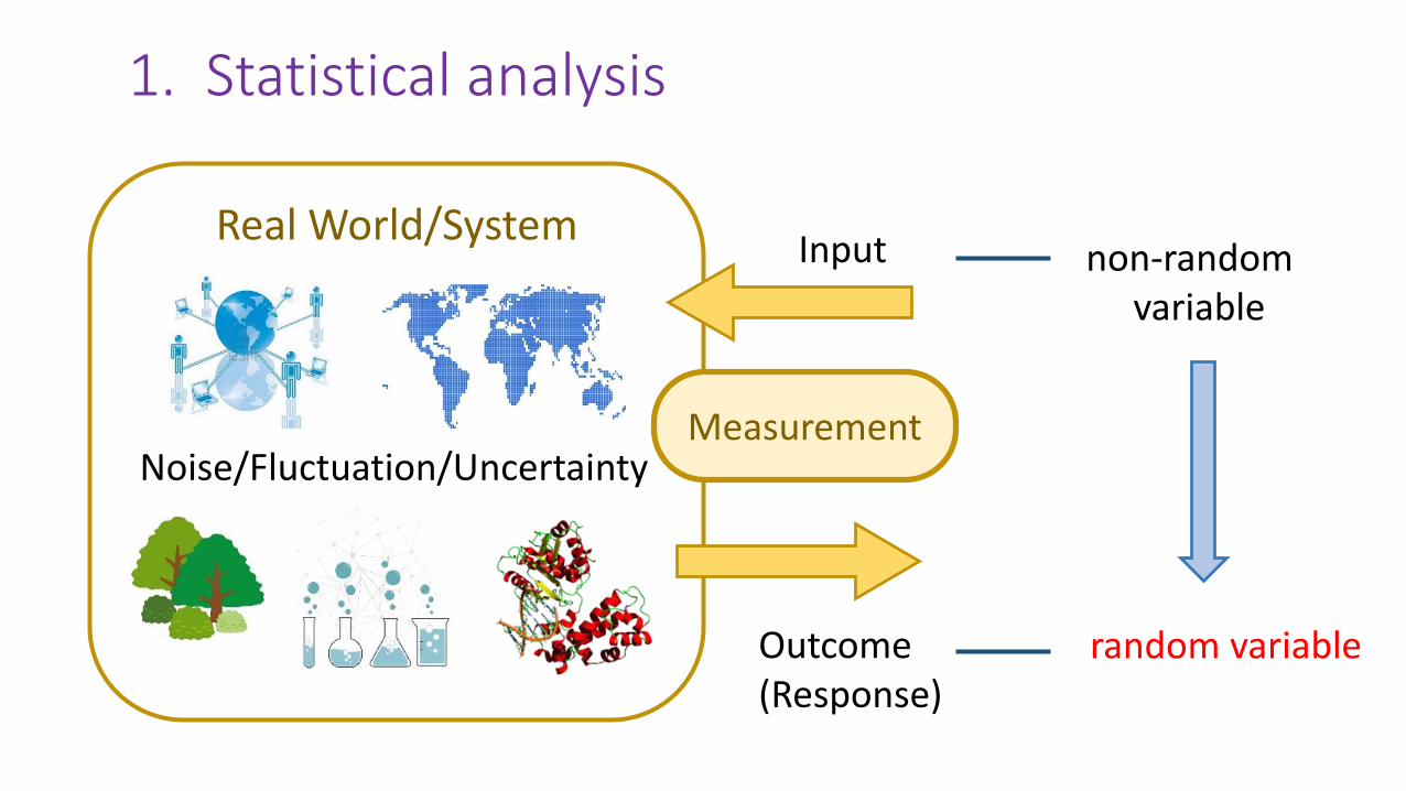
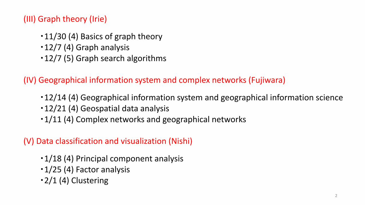
1. Statistical analysis

Real World/System

Noise/Fluctuation/Uncertainty

Input

Outcome(Response)

Measurement

non-random variable

random variable

2. Random variables

7

𝑥

𝑋

A random variable 𝑋 varies over a domain in the real linewith certain tendency (probability)of occurrence of its values.

• discrete random variable

• continuous random variable

3. Probability distributions I: Discrete case

• range of values {𝑎1, 𝑎2, … , 𝑎𝑛, … }

• distribution by a sum of point masses

𝑃 𝑋 = 𝑎𝑛 = 𝑝𝑛, 𝑝𝑛≥ 0,

𝑛

𝑝𝑛 = 1

• mean value

𝑚 = 𝑚𝑋 = 𝐄 𝑋 =

𝑛

𝑎𝑛 𝑝𝑛

• variance

𝜎2 = 𝜎𝑋2 = 𝐕 𝑋 = 𝐄 𝑋 −𝑚 2 =

𝑛

𝑎𝑛 −𝑚 2 𝑝𝑛

= 𝐄 𝑋2 −𝑚2 =

𝑛

𝑎𝑛2 𝑝𝑛 −𝑚2

8

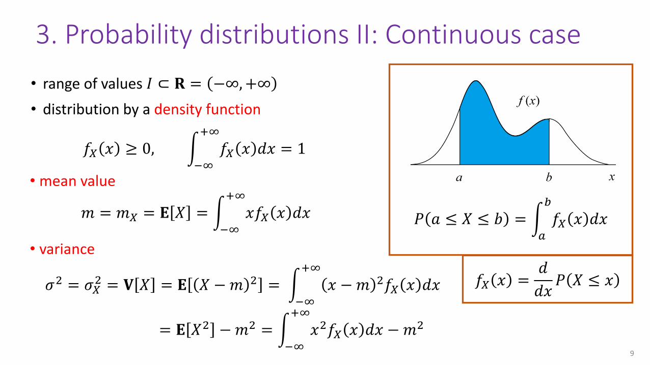
3. Probability distributions II: Continuous case

• range of values 𝐼 ⊂ 𝐑 = −∞,+∞

• distribution by a density function

9

𝑓𝑋 𝑥 ≥ 0, න−∞

+∞

𝑓𝑋 𝑥 𝑑𝑥 = 1

• mean value

𝑚 = 𝑚𝑋 = 𝐄 𝑋 = න−∞

+∞

𝑥𝑓𝑋 𝑥 𝑑𝑥

• variance

𝜎2 = 𝜎𝑋2 = 𝐕 𝑋 = 𝐄 𝑋 −𝑚 2 = න

−∞

+∞

𝑥 − 𝑚 2𝑓𝑋 𝑥 𝑑𝑥

= 𝐄 𝑋2 −𝑚2 = න−∞

+∞

𝑥2𝑓𝑋 𝑥 𝑑𝑥 −𝑚2

𝑃 𝑎 ≤ 𝑋 ≤ 𝑏 = න𝑎

𝑏

𝑓𝑋 𝑥 𝑑𝑥

𝑓𝑋 𝑥 =𝑑

𝑑𝑥𝑃 𝑋 ≤ 𝑥

3. Probability distributions: A listDiscrete distributions mean variance

binomial distribution 𝐵(𝑛,𝑝) 𝑛𝑝 𝑛𝑝 1 − 𝑝

Bernoulli distribution 𝐵(1,𝑝) 𝑝 𝑝 1 − 𝑝

geometric distribution with parameter 𝑝 1/𝑝 1/𝑝2

Poisson distribution with parameter 𝜆 Po(𝜆) 𝜆 𝜆

Continuous distributions mean variance

uniform distribution on [𝑎,𝑏] 𝑎 + 𝑏 /2 𝑏 − 𝑎 2/12

exponential distribution with parameter 𝜆 1/𝜆 1/𝜆2

normal (or Gaussian) distribution 𝑁(𝑚, 𝜎2) 𝑚 𝜎2

chi-square distribution 𝜒𝑛2

𝑛 2𝑛

𝑡-distribution 𝑡𝑛 0 𝑛/(𝑛 − 2)

F-distribution 𝐹 𝑚, 𝑛 = 𝐹𝑛𝑚 𝑛/ 𝑛 − 2 2𝑛2 𝑚+ 𝑛 − 2

/𝑚 𝑛 − 2 2 𝑛 − 4

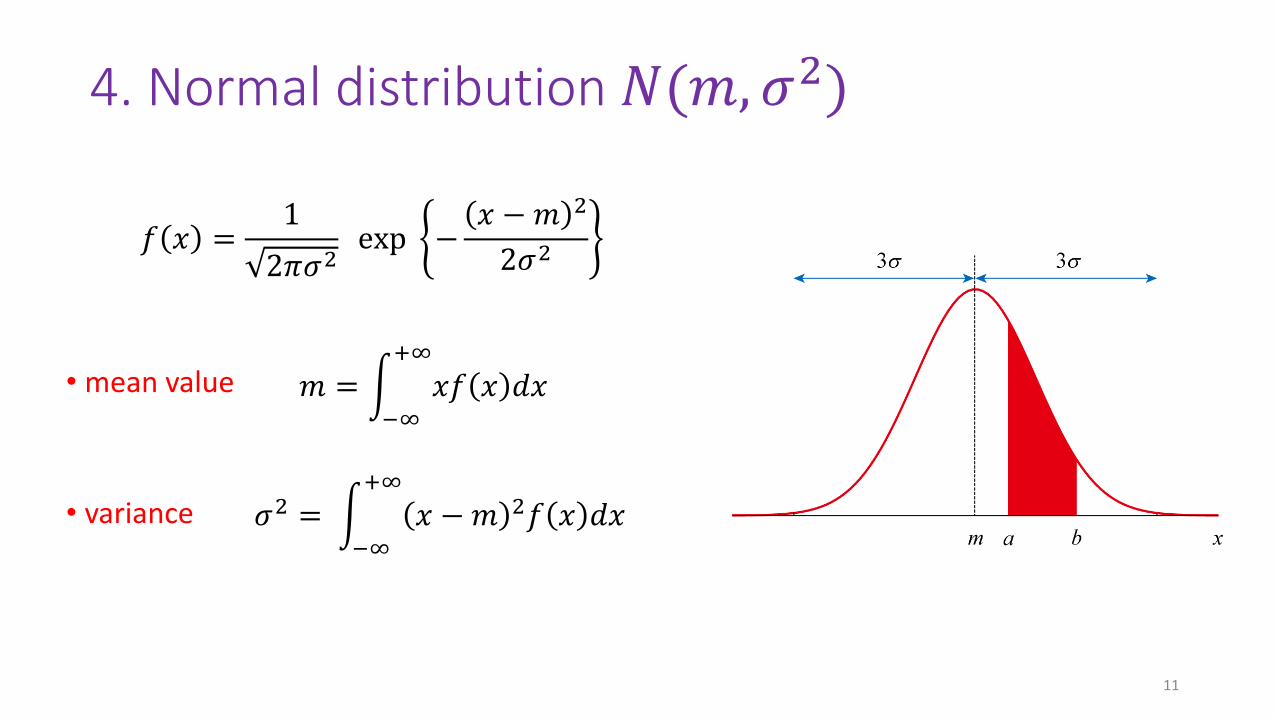
4. Normal distribution 𝑁(𝑚, 𝜎2)

11

𝑓 𝑥 =1

2𝜋𝜎2exp −

𝑥 −𝑚 2

2𝜎2

𝑚 = න−∞

+∞

𝑥𝑓 𝑥 𝑑𝑥

𝜎2 = න−∞

+∞

𝑥 −𝑚 2𝑓 𝑥 𝑑𝑥

• mean value

• variance

5. Central Limit Theorem (CLT)

12

𝑍1, 𝑍2, ⋯ , 𝑍𝑛, ⋯ : independent identically distributed (iid) random variables

mean value = 𝑚, variance = 𝜎2

𝑆𝑛 −𝑚𝑛 ~ 𝑁 0, 𝑛𝜎2CLT holds as 𝑛 → ∞

• Accumulation of small fluctuation gives rise to a normal distribution.

Consider the sum:

𝑆𝑛 = 𝑍1 + 𝑍2 +⋯+ 𝑍𝑛 =

𝑘=1

𝑛

𝑍𝑘

𝑍1 𝑍2 𝑍3 𝑍4 𝑍𝑛⋯

𝐄 𝑆𝑛 =

𝑘=1

𝑛

𝐄 𝑍𝑘 = 𝑚𝑛

mean value

6. An example of data

13

Two sets of numerical data are shown in the following table.- dried weight of plants grown under two conditions

Is there any significant difference?

A4.81 4.17 4.41 3.59 5.87 3.83 6.03 4.98 4.90 5.75

5.36 3.48 4.69 4.44 4.89 4.71 5.48 4.32 5.15 6.34

B4.17 3.05 5.18 4.01 6.11 4.10 5.17 3.57 5.33 5.59

4.66 5.58 3.66 4.50 3.90 4.61 5.62 4.53 6.05 5.14

[Dobson] Exercise 2.1

Details Later

14

A4.81 4.17 4.41 3.59 5.87 3.83 6.03 4.98 4.90 5.75

5.36 3.48 4.69 4.44 4.89 4.71 5.48 4.32 5.15 6.34

B4.17 3.05 5.18 4.01 6.11 4.10 5.17 3.57 5.33 5.59

4.66 5.58 3.66 4.50 3.90 4.61 5.62 4.53 6.05 5.14

A biological system

• noise• fluctuation

By empirical knowledge 𝑋is often assumed to obey a normal distribution[see also CLT].

𝑋 ~ 𝑁(𝑚, 𝜎2)

just one of the possible values of 𝑋𝑘

𝑋𝑘 : 𝑘 th output

𝑥𝑘 : 𝑘 th data

Input Outcome

𝑋

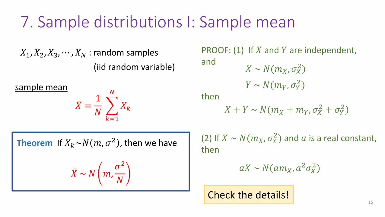
7. Sample distributions I: Sample mean

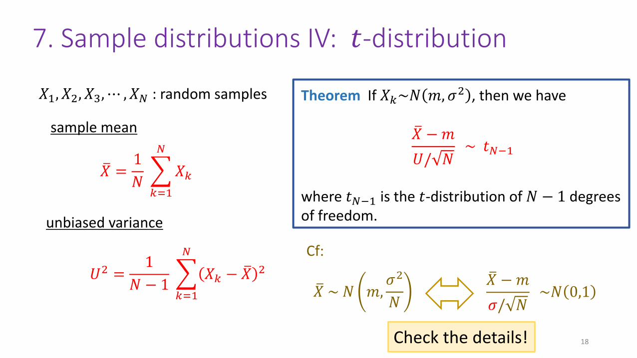
𝑋1, 𝑋2, 𝑋3, ⋯ , 𝑋𝑁 : random samples

(iid random variable)

Theorem If 𝑋𝑘~𝑁 𝑚, 𝜎2 , then we have

ത𝑋 ~ 𝑁 𝑚,𝜎2

𝑁

15

PROOF: (1) If 𝑋 and 𝑌 are independent,and

then

𝑋 ~ 𝑁(𝑚𝑋, 𝜎𝑋2)

𝑌 ~ 𝑁(𝑚𝑌, 𝜎𝑌2)

𝑋 + 𝑌 ~ 𝑁(𝑚𝑋 +𝑚𝑌, 𝜎𝑋2 + 𝜎𝑌

2)

(2) If 𝑋 ~ 𝑁(𝑚𝑋, 𝜎𝑋2) and 𝑎 is a real constant,

then

𝑎𝑋 ~ 𝑁(𝑎𝑚𝑋, 𝑎2𝜎𝑋

2)

ത𝑋 =1

𝑁

𝑘=1

𝑁

𝑋𝑘

sample mean

Check the details!

7. Sample distributions II: Unbiased variance

𝑋1, 𝑋2, 𝑋3, ⋯ , 𝑋𝑁 : random samples Theorem If 𝑋𝑘~𝑁 𝑚, 𝜎2 , then we have

𝑁 − 1

𝜎2𝑈2 ~ 𝜒𝑁−1

2

16

Theorem If 𝑋1, 𝑋2, 𝑋3, ⋯ , 𝑋𝑁 are iidrandom variable with mean 𝑚 and variance 𝜎2, we have

𝐄 ത𝑋 = 𝑚, 𝐄 𝑈2 = 𝜎2

𝑈2 =1

𝑁 − 1

𝑘=1

𝑁

𝑋𝑘 − ത𝑋 2

unbiased variance

Here 𝜒𝑁−12 is the chi-square distribution of

𝑁 − 1 degrees of freedom.

• Sum of squares appears in many contexts.

𝑘=1

𝑁

𝑋𝑘 − ത𝑋 2

Check the details!

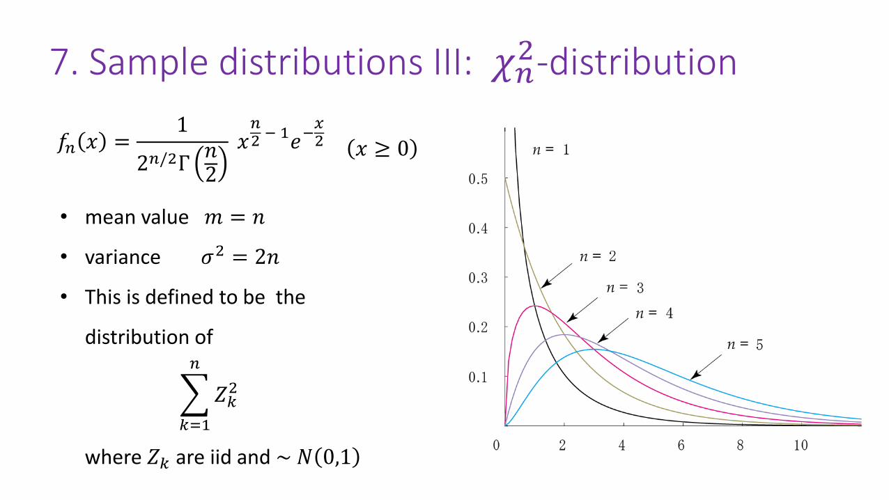
7. Sample distributions III: 𝜒𝑛2-distribution

𝑓𝑛 𝑥 =1

2𝑛/2Γ𝑛2

𝑥𝑛2 − 1𝑒−

𝑥2 𝑥 ≥ 0

• mean value 𝑚 = 𝑛

• variance 𝜎2 = 2𝑛

• This is defined to be the

distribution of

where 𝑍𝑘 are iid and ~ 𝑁 0,1

𝑘=1

𝑛

𝑍𝑘2

𝑋1, 𝑋2, 𝑋3, ⋯ , 𝑋𝑁 : random samples Theorem If 𝑋𝑘~𝑁 𝑚, 𝜎2 , then we have

ത𝑋 −𝑚

𝑈/ 𝑁~ 𝑡𝑁−1

where 𝑡𝑁−1 is the 𝑡-distribution of 𝑁 − 1 degrees of freedom.

18

𝑈2 =1

𝑁 − 1

𝑘=1

𝑁

𝑋𝑘 − ത𝑋 2

ത𝑋 =1

𝑁

𝑘=1

𝑁

𝑋𝑘

sample mean

unbiased variance

7. Sample distributions IV: 𝑡-distribution

Check the details!

ത𝑋 ~ 𝑁 𝑚,𝜎2

𝑁

ത𝑋 −𝑚

𝜎/ 𝑁~𝑁 0,1

Cf:

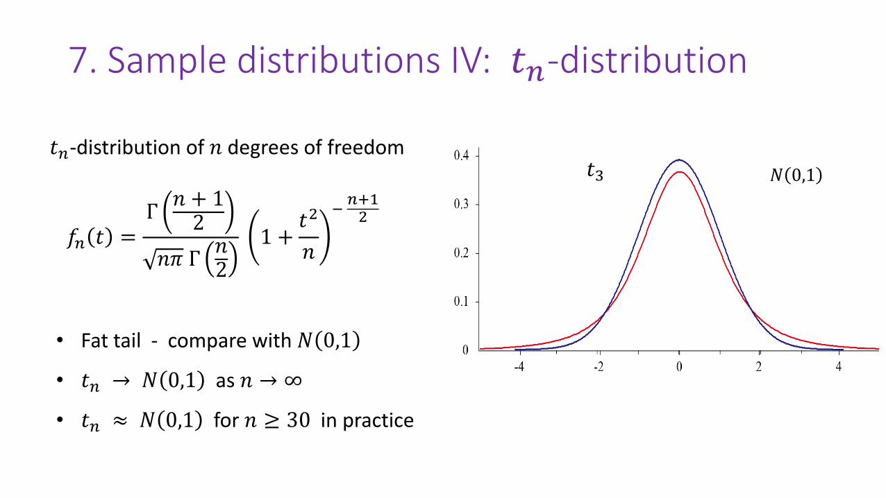
• Fat tail - compare with 𝑁 0,1

• 𝑡𝑛 → 𝑁 0,1 as 𝑛 → ∞

• 𝑡𝑛 ≈ 𝑁 0,1 for 𝑛 ≥ 30 in practice

𝑡𝑛-distribution of 𝑛 degrees of freedom

𝑓𝑛 𝑡 =Γ𝑛 + 12

𝑛𝜋 Γ𝑛2

1 +𝑡2

𝑛

−𝑛+12

𝑡3 𝑁 0,1

7. Sample distributions IV: 𝑡𝑛-distribution

8. Random vectors

20

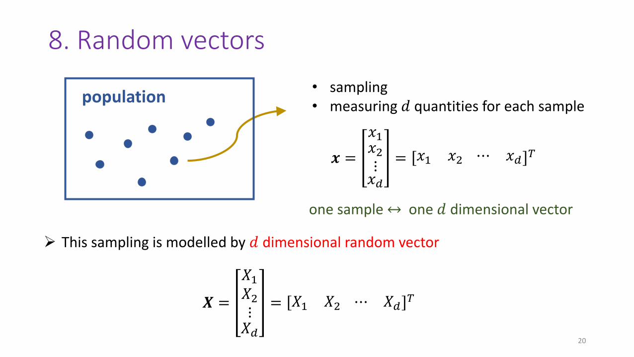
• sampling• measuring 𝑑 quantities for each sample

𝒙 =

𝑥1𝑥2⋮𝑥𝑑

= 𝑥1 𝑥2 ⋯ 𝑥𝑑 𝑇

one sample ↔ one 𝑑 dimensional vector

population

𝑿 =

𝑋1𝑋2⋮𝑋𝑑

= 𝑋1 𝑋2 ⋯ 𝑋𝑑𝑇

➢ This sampling is modelled by 𝑑 dimensional random vector

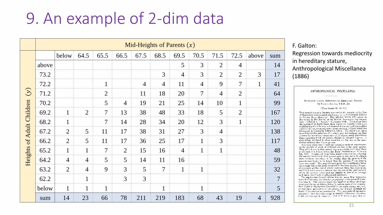
9. An example of 2-dim data

Mid-Heights of Parents 𝑥

Hei

gh

ts o

f A

du

lt C

hil

dre

n

below 64.5 65.5 66.5 67.5 68.5 69.5 70.5 71.5 72.5 above sum

above 5 3 2 4 14

73.2 3 4 3 2 2 3 17

72.2 1 4 4 11 4 9 7 1 41

71.2 2 11 18 20 7 4 2 64

70.2 5 4 19 21 25 14 10 1 99

69.2 1 2 7 13 38 48 33 18 5 2 167

68.2 1 7 14 28 34 20 12 3 1 120

67.2 2 5 11 17 38 31 27 3 4 138

66.2 2 5 11 17 36 25 17 1 3 117

65.2 1 1 7 2 15 16 4 1 1 48

64.2 4 4 5 5 14 11 16 59

63.2 2 4 9 3 5 7 1 1 32

62.2 1 3 3 7

below 1 1 1 1 1 5

sum 14 23 66 78 211 219 183 68 43 19 4 928

F. Galton:Regression towards mediocrity in hereditary stature, Anthropological Miscellanea (1886)

21

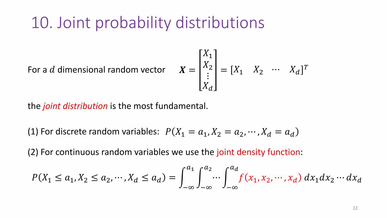
10. Joint probability distributions

the joint distribution is the most fundamental.

(1) For discrete random variables: 𝑃 𝑋1 = 𝑎1, 𝑋2 = 𝑎2, ⋯ , 𝑋𝑑 = 𝑎𝑑

(2) For continuous random variables we use the joint density function:

𝑃 𝑋1 ≤ 𝑎1, 𝑋2 ≤ 𝑎2, ⋯ , 𝑋𝑑 ≤ 𝑎𝑑 = න−∞

𝑎1

න−∞

𝑎2

⋯න−∞

𝑎𝑑

𝑓 𝑥1, 𝑥2, ⋯ , 𝑥𝑑 𝑑𝑥1𝑑𝑥2⋯𝑑𝑥𝑑

For a 𝑑 dimensional random vector

22

𝑿 =

𝑋1𝑋2⋮𝑋𝑑

= 𝑋1 𝑋2 ⋯ 𝑋𝑑𝑇

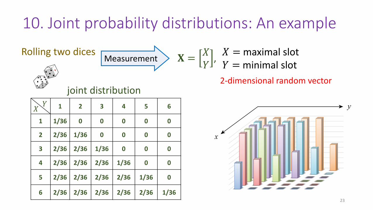
10. Joint probability distributions: An example

1 2 3 4 5 6

1 1/36 0 0 0 0 0

2 2/36 1/36 0 0 0 0

3 2/36 2/36 1/36 0 0 0

4 2/36 2/36 2/36 1/36 0 0

5 2/36 2/36 2/36 2/36 1/36 0

6 2/36 2/36 2/36 2/36 2/36 1/36

𝑋𝑌

joint distribution

23

Measurement 𝐗 =𝑋𝑌

,𝑋 = maximal slot𝑌 = minimal slot

2-dimensional random vector

Rolling two dices

10. Joint probability distributions: 𝑁 𝒎, Σ

• 2-dimensional case 𝑁 𝒎, Σ

𝑓 𝑥 =1

2𝜋𝜎2exp −

𝑥 −𝑚 2

2𝜎2

• 1-dimensional case 𝑁 𝑚, 𝜎2

24

𝑓 𝑥, 𝑦 = ⋯

Details Later

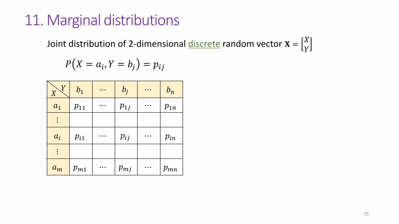
𝑏1 ⋯ 𝑏𝑗 ⋯ 𝑏𝑛

𝑎1 𝑝11 ⋯ 𝑝1𝑗 ⋯ 𝑝1𝑛

⋮

𝑎𝑖 𝑝𝑖1 ⋯ 𝑝𝑖𝑗 ⋯ 𝑝𝑖𝑛

⋮

𝑎𝑚 𝑝𝑚1 ⋯ 𝑝𝑚𝑗 ⋯ 𝑝𝑚𝑛

11. Marginal distributions

𝑋𝑌

25

Joint distribution of 2-dimensional discrete random vector 𝐗 = 𝑋𝑌

𝑃 𝑋 = 𝑎𝑖 , 𝑌 = 𝑏𝑗 = 𝑝𝑖𝑗

𝑏1 ⋯ 𝑏𝑗 ⋯ 𝑏𝑛 sum

𝑎1 𝑝11 ⋯ 𝑝1𝑗 ⋯ 𝑝1𝑛 𝑝1∙

⋮

𝑎𝑖 𝑝𝑖1 ⋯ 𝑝𝑖𝑗 ⋯ 𝑝𝑖𝑛 𝑝𝑖∙

⋮

𝑎𝑚 𝑝𝑚1 ⋯ 𝑝𝑚𝑗 ⋯ 𝑝𝑚𝑛 𝑝𝑚∙

11. Marginal distributions

𝑋𝑌

26

𝑃 𝑋 = 𝑎𝑖 , 𝑌 = 𝑏𝑗 = 𝑝𝑖𝑗

𝑃 𝑋 = 𝑎𝑖 =

𝑗=1

𝑛

𝑃 𝑋 = 𝑎𝑖 , 𝑌 = 𝑏𝑗

Marginal distribution

Joint distribution of 2-dimensional discrete random vector 𝐗 = 𝑋𝑌

𝑏1 ⋯ 𝑏𝑗 ⋯ 𝑏𝑛 sum

𝑎1 𝑝11 ⋯ 𝑝1𝑗 ⋯ 𝑝1𝑛 𝑝1∙

⋮

𝑎𝑖 𝑝𝑖1 ⋯ 𝑝𝑖𝑗 ⋯ 𝑝𝑖𝑛 𝑝𝑖∙

⋮

𝑎𝑚 𝑝𝑚1 ⋯ 𝑝𝑚𝑗 ⋯ 𝑝𝑚𝑛 𝑝𝑚∙

sum 𝑝∙1 𝑝∙𝑗 𝑝∙𝑛 1

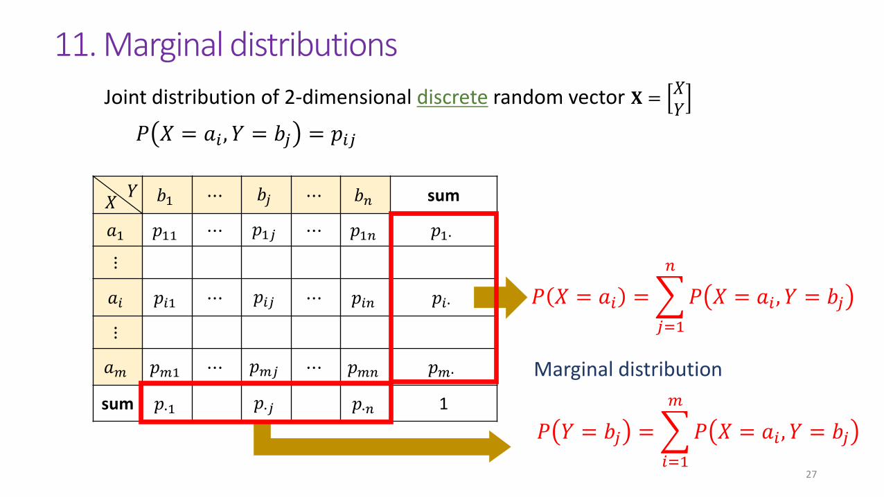
11. Marginal distributions

𝑋𝑌

27

𝑃 𝑋 = 𝑎𝑖 , 𝑌 = 𝑏𝑗 = 𝑝𝑖𝑗

𝑃 𝑋 = 𝑎𝑖 =

𝑗=1

𝑛

𝑃 𝑋 = 𝑎𝑖 , 𝑌 = 𝑏𝑗

Marginal distribution

𝑃 𝑌 = 𝑏𝑗 =

𝑖=1

𝑚

𝑃 𝑋 = 𝑎𝑖 , 𝑌 = 𝑏𝑗

Joint distribution of 2-dimensional discrete random vector 𝐗 = 𝑋𝑌

𝑏1 ⋯ 𝑏𝑗 ⋯ 𝑏𝑛 sum

𝑎1 𝑝1𝑗

⋮ ⋮

𝑎𝑖 𝑝𝑖𝑗

⋮ ⋮

𝑎𝑚 𝑝𝑚𝑗

sum 𝑃 𝑌 = 𝑏𝑗 1

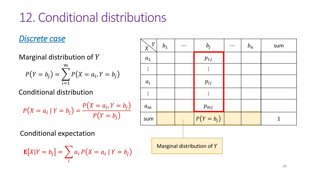
12. Conditional distributions

𝑋𝑌

Marginal distribution of 𝑌

Discrete case

28

𝑃 𝑌 = 𝑏𝑗 =

𝑖=1

𝑚

𝑃 𝑋 = 𝑎𝑖 , 𝑌 = 𝑏𝑗

Marginal distribution of 𝑌

𝑃 𝑋 = 𝑎𝑖 | 𝑌 = 𝑏𝑗 =𝑃 𝑋 = 𝑎𝑖 , 𝑌 = 𝑏𝑗

𝑃 𝑌 = 𝑏𝑗

Conditional distribution

Conditional expectation

𝐄 𝑋|𝑌 = 𝑏𝑗 =

𝑖

𝑎𝑖 𝑃 𝑋 = 𝑎𝑖 | 𝑌 = 𝑏𝑗

Exercise 1 (5min)

Suppose that the joint distribution of 𝑋, 𝑌 is given by the following table:

1 2 3 4

1 1/16 1/16 0 0

2 1/16 2/16 0 1/16

3 2/16 2/16 0 1/16

4 1/16 1/16 2/16 1/16

𝑋𝑌

(1) Find the marginal distributions.

(2) Calculate 𝐄 𝑋 and 𝐕 𝑋 .

(3) Find 𝑃 𝑋 = 2|𝑌 = 1 .

(4) Find 𝑃 𝑌 = 2|𝑋 = 3 .

(5) Find 𝐄 𝑌|𝑋 = 3 .

29

14. Covariance and correlation coefficient

Normalization of a random variable:

30

𝜌 𝑋, 𝑌 =𝐂𝐨𝐯 𝑋, 𝑌

𝑉 𝑋 𝑉 𝑌=

𝜎𝑋𝑌𝜎𝑋𝜎𝑌

𝐂𝐨𝐯 𝑋, 𝑌 = 𝐄 𝑋 − 𝐄 𝑋 𝑌 − 𝐄 𝑌

= 𝐄 𝑋𝑌 − 𝐄 𝑋 𝐄 𝑌

෨𝑋 =𝑋 − 𝐄 𝑋

𝑉 𝑋=𝑋 −𝑚

𝜎

𝐸 ෨𝑋 = 0, 𝑉 ෨𝑋 = 1 𝜌 𝑋, 𝑌 = 𝐸 ෨𝑋 ෨𝑌 = 𝐂𝐨𝐯 ෨𝑋, ෨𝑌 = 𝜌 ෨𝑋, ෨𝑌

FORMULA:Check the details!

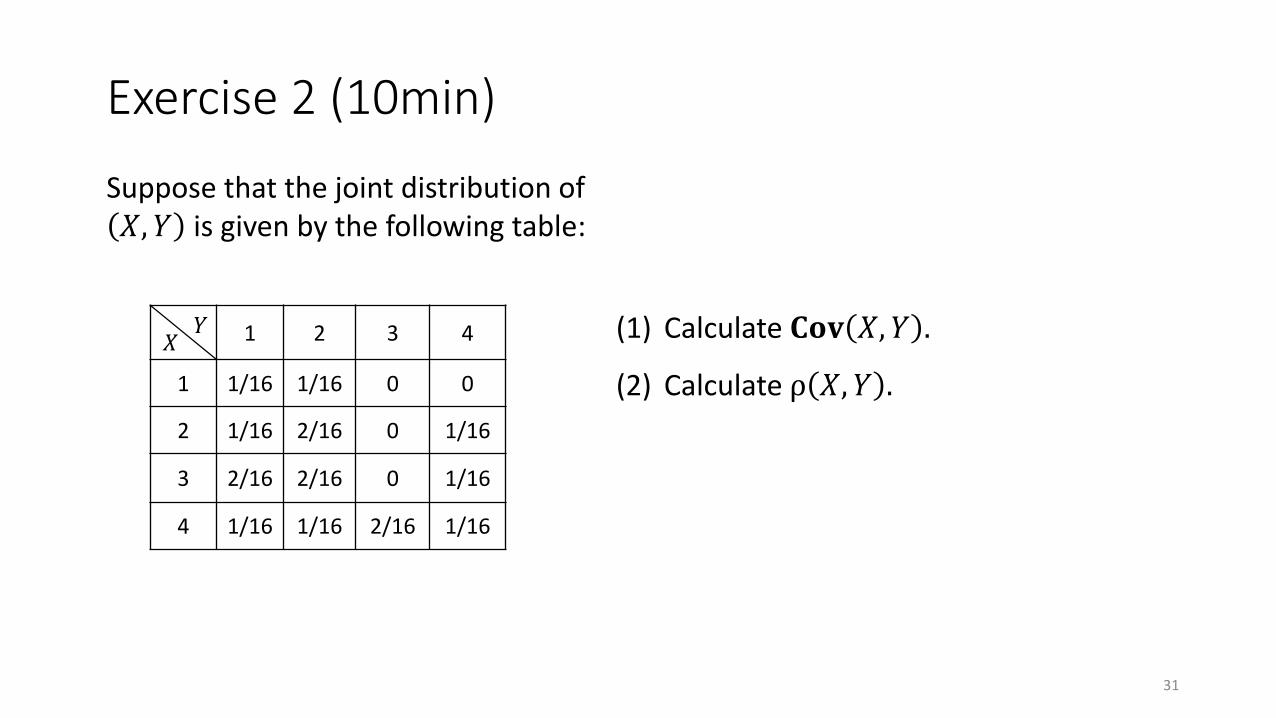
Exercise 2 (10min)

Suppose that the joint distribution of 𝑋, 𝑌 is given by the following table:

1 2 3 4

1 1/16 1/16 0 0

2 1/16 2/16 0 1/16

3 2/16 2/16 0 1/16

4 1/16 1/16 2/16 1/16

𝑋𝑌 (1) Calculate 𝐂𝐨𝐯 𝑋, 𝑌 .

(2) Calculate ρ 𝑋, 𝑌 .

31

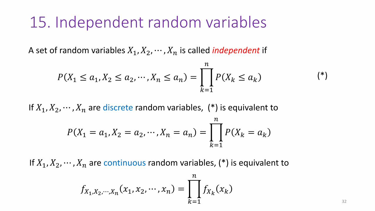
15. Independent random variables

If 𝑋1, 𝑋2, ⋯ , 𝑋𝑛 are discrete random variables, (*) is equivalent to

𝑃 𝑋1 = 𝑎1, 𝑋2 = 𝑎2, ⋯ , 𝑋𝑛 = 𝑎𝑛 =ෑ

𝑘=1

𝑛

𝑃 𝑋𝑘 = 𝑎𝑘

A set of random variables 𝑋1, 𝑋2, ⋯ , 𝑋𝑛 is called independent if

𝑃 𝑋1 ≤ 𝑎1, 𝑋2 ≤ 𝑎2, ⋯ , 𝑋𝑛 ≤ 𝑎𝑛 =ෑ

𝑘=1

𝑛

𝑃 𝑋𝑘 ≤ 𝑎𝑘 (*)

If 𝑋1, 𝑋2, ⋯ , 𝑋𝑛 are continuous random variables, (*) is equivalent to

𝑓𝑋1,𝑋2,⋯,𝑋𝑛 𝑥1, 𝑥2, ⋯ , 𝑥𝑛 =ෑ

𝑘=1

𝑛

𝑓𝑋𝑘 𝑥𝑘32

PROOF (1) We deal with discrete random variables. For continuous case we need only to replace the joint probability by joint density function.

𝐄 𝑎𝑋 + 𝑏𝑌 =

𝑧

𝑧𝑃 𝑎𝑋 + 𝑏𝑌 = 𝑧 =

𝑧

𝑧

𝑎𝑥+𝑏𝑦=𝑧

𝑃 𝑋 = 𝑥, 𝑌 = 𝑦 =

𝑥,𝑦

𝑎𝑥 + 𝑏𝑦 𝑃 𝑋 = 𝑥, 𝑌 = 𝑦

= 𝑎

𝑥,𝑦

𝑥𝑃 𝑋 = 𝑥, 𝑌 = 𝑦 + 𝑏

𝑥,𝑦

𝑦𝑃 𝑋 = 𝑥, 𝑌 = 𝑦 =𝑎𝐄 𝑋 + 𝑏𝐄 𝑌

(2) By definition,

𝐕 𝑎𝑋 + 𝑏𝑌 = 𝐄 𝑎𝑋 + 𝑏𝑌 2 − 𝐄 𝑎𝑋 + 𝑏𝑌 2

= 𝑎2 𝐄 𝑋2 + 2𝑎𝑏𝐄 𝑋𝑌 + 𝑏2𝐄 𝑌2 − 𝑎2𝐄 𝑋 2 − 2𝑎𝑏𝐄 𝑋 𝐄 𝑌 − 𝑏2𝐄 𝑌 2

= 𝑎2𝐕 𝑋 + 𝑏2𝐕 𝑌 + 2𝑎𝑏𝐂𝐨𝐯 𝑋, 𝑌

(2) 𝐕 𝑎𝑋 + 𝑏𝑌 = 𝑎2𝐕 𝑋 + 𝑏2𝐕 𝑌 + 2𝑎𝑏𝐂𝐨𝐯 𝑋, 𝑌

(1) 𝐄 𝑎𝑋 + 𝑏𝑌 = 𝑎𝐄 𝑋 + 𝑏𝐄 𝑌

FORMULA: For any random variables 𝑋 and 𝑌, we have

33

Check the details!

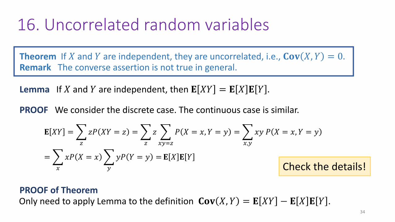
16. Uncorrelated random variables

Remark The converse assertion is not true in general.

PROOF of Theorem Only need to apply Lemma to the definition 𝐂𝐨𝐯 𝑋, 𝑌 = 𝐄 𝑋𝑌 − 𝐄 𝑋 𝐄 𝑌 .

Lemma If 𝑋 and 𝑌 are independent, then 𝐄 𝑋𝑌 = 𝐄 𝑋 𝐄 𝑌 .

PROOF We consider the discrete case. The continuous case is similar.

𝐄 𝑋𝑌 =

𝑧

𝑧𝑃 𝑋𝑌 = 𝑧 =

𝑧

𝑧

𝑥𝑦=𝑧

𝑃 𝑋 = 𝑥, 𝑌 = 𝑦 =

𝑥,𝑦

𝑥𝑦 𝑃 𝑋 = 𝑥, 𝑌 = 𝑦

=

𝑥

𝑥𝑃 𝑋 = 𝑥

𝑦

𝑦𝑃 𝑌 = 𝑦 =𝐄 𝑋 𝐄 𝑌

34

Check the details!

Theorem If 𝑋 and 𝑌 are independent, they are uncorrelated, i.e., 𝐂𝐨𝐯 𝑋, 𝑌 = 0.

✓ During my lectures you will be given 10 Problems.

✓ Choose 3 problems at your own taste and write up a short report.

✓ Submission deadline: November 5 (Mon), 2018.

✓ Way of submission: (a) directly hand to Prof Obata

or (b) send in PDF by e-mail to obata@tohoku.ac.jp

or (c) bring to the secretary on 6F GSIS and ask her politely.

Submission of reports for evaluation

35

Problem 1

Suppose that the joint distribution of 𝑋, 𝑌 is given by the following table:

1 2 3 4 5 6

1 1/36 0 0 0 0 0

2 2/36 1/36 0 0 0 0

3 2/36 2/36 1/36 0 0 0

4 2/36 2/36 2/36 1/36 0 0

5 2/36 2/36 2/36 2/36 1/36 0

6 2/36 2/36 2/36 2/36 2/36 1/36

𝑋𝑌

(1) Find the marginal distributions.

(2) Calculate 𝐄 𝑋 and 𝐕 𝑋 .

(3) Calculate 𝐂𝐨𝐯 𝑋, 𝑌 and ρ 𝑋, 𝑌 .

(4) Find 𝑃 𝑋 = 4|𝑌 = 2 .

(5) Find 𝐄 𝑋|𝑌 = 2 .

(6) [challenge] Since 𝐄[𝑋|𝑌=𝑘] (𝑘 =

1,2,⋯ , 6) may be considered as a

function of 𝑌, it is a random variable,

denoted by 𝐄[𝑋|𝑌] and called the

conditional expectation. Examine that

𝐄[𝐄[𝑋|𝑌]]=𝐄[𝑋].36

Problem 2

Four cards are drawn from a deck (of 52 cards). Let 𝑋 be the number of acesand 𝑌 the number of kings that show.

(1) Show the joint distribution of 𝑋, 𝑌 , and marginal distributions of 𝑋 and 𝑌.

(2) Find the mean values 𝐄 𝑋 and 𝐄 𝑌 .

(3) Find the variances 𝐕 𝑋 and 𝐕 𝑌 .

(4) Find the covariance 𝐂𝐨𝐯 𝑋, 𝑌 and correlation coefficient 𝜌 𝑋, 𝑌 .

(5) Find 𝐄 𝑋|𝑌 = 1

➢ Answer by the ratios of integers, do not use decimal expressions.

37

Problem 3

Let 𝑋, 𝑌 be random variables taking just two values, say,

𝑃 𝑋 = 𝑎 = 𝑝, 𝑃 𝑋 = 𝑏 = 1 − 𝑝

𝑃 𝑌 = 𝑐 = 𝑞, 𝑃 𝑌 = 𝑑 = 1 − 𝑞

0 < 𝑝 < 1, 0 < 𝑞 < 1.

Show that 𝑋 and 𝑌 are independent if and only if 𝐂𝐨𝐯 𝑋, 𝑌 = 0.

Note: ‘only if’ part is straightforward (see also the general theorem in Section 16). The point here is to show ‘if’ part.

Problem 4

39

A4.81 4.17 4.41 3.59 5.87 3.83 6.03 4.98 4.90 5.75

5.36 3.48 4.69 4.44 4.89 4.71 5.48 4.32 5.15 6.34

B4.17 3.05 5.18 4.01 6.11 4.10 5.17 3.57 5.33 5.59

4.66 5.58 3.66 4.50 3.90 4.61 5.62 4.53 6.05 5.14

(1) Show the histogram of each group.

(2) Calculate the mean value and unbiased variance of each group.

(3) Judge by hypothesis testing whether these groups are random samples

from the normal population 𝑁 4.82,0.04 =N 4.82,0.22 ?

➢ If you are not familiar with the hypothesis testing, study it on this occasion!