Data Processing Report - Mineral Resources Tasmania · 2018-05-11 · WesternGeco T/32P & T/33P, Sorell Basin 2D S c h l u m b e r g e r P r i v a t e 1.0 Introduction This report

Data Processing Report

for

Area: Sorell Basin SS02

Permits: T/32P, T/33P

WG Contract Number: J2663

Date: October 2003

Level 5, 256 St Georges Terrace, Perth 6000, Western Australia

Report Authors Alison Keighley and Kenneth Jayan

WesternGeco T/32P & T/33P, Sorell Basin 2D

Schlumberger Private

Table of Contents

1.0 INTRODUCTION ................................................................................................................................4

2.0 TESTING ..............................................................................................................................................5

3.0 PRE-STACK SEISMIC DATA PROCESSING ................................................................................6 3.1 REFORMAT ....................................................................................................................................6 3.2 LINE MERGING...............................................................................................................................6 3.3 MARINE 2D GEOMETRY ................................................................................................................6 3.4 GUN AND CABLE CORRECTION .....................................................................................................6 3.5 LOW-CUT FILTER...........................................................................................................................7 3.6 PRELIMINARY 8KM VELOCITY ANALYSIS......................................................................................7 3.7 COMMON RECEIVER POINT GATHER .............................................................................................7 3.8 SWELL NOISE ATTENUATION (SWATT) .......................................................................................7 3.9 COMMON SHOT POINT GATHER ....................................................................................................9 3.10 F-K DIP FILTER .............................................................................................................................9 3.11 RESAMPLE...................................................................................................................................11 3.12 PRESTACK SHOT INTERPOLATION (2.5D) ....................................................................................11 3.13 K-FILTER / TRACE REDUCTION ...................................................................................................11 3.14 COMMON MID POINT GATHER ....................................................................................................12 3.15 2KM VELOCITY ANALYSIS ..........................................................................................................12 3.16 RADON MULTIPLE ATTENUATION ...............................................................................................13 3.17 DATA REDUCTION.......................................................................................................................16 3.18 MARINE 2D GEOMETRY ..............................................................................................................16 3.19 1KM VELOCITY ANALYSIS ..........................................................................................................16 3.20 TVF ............................................................................................................................................16 3.21 KIRCHHOFF PRE-STACK TIME MIGRATION .................................................................................17 3.22 GEOMETRIC SPREADING AMPLITUDE COMPENSATION................................................................19 3.23 FINAL 500M VELOCITY ANALYSIS..............................................................................................19 3.24 NORMAL MOVEOUT ....................................................................................................................19 3.25 RADON MULTIPLE ATTENUATION ...............................................................................................20 3.26 CMP GATHER ARCHIVE...............................................................................................................20 3.27 SCALING (INSTANTANEOUS GAIN) ..............................................................................................20 3.28 MUTE ..........................................................................................................................................21

3.28.1 Inner Trace Mute ................................................................................................................21 3.28.2 Outer Trace Mute ...............................................................................................................21

3.29 STACK .........................................................................................................................................23 3.30 WATER BOTTOM TIME UPDATE ..................................................................................................23 3.31 NAVIGATION/SEISMIC DATA MERGE............................................................................................23 3.32 DATA ARCHIVE ...........................................................................................................................23

4.0 POST-STACK SEISMIC DATA PROCESSING............................................................................24 4.1 TAU-P COHERENCY FILTER.........................................................................................................24 4.2 TRACE MIX ..................................................................................................................................24 4.3 TVF ............................................................................................................................................25 4.4 SCALING (CASCADED INSTANTANEOUS GAIN)............................................................................26 4.5 CGM FILES .................................................................................................................................26 4.6 DATA ARCHIVE ...........................................................................................................................26 4.7 ANGLE STACKS ...........................................................................................................................26

4.7.1 Near angle stack .................................................................................................................26 4.7.2 Far angle stack ..................................................................................................................26

4.8 DATA ARCHIVE ...........................................................................................................................27 5.0 PERSONNEL......................................................................................................................................28

6.0 APPENDICES ....................................................................................................................................29 6.1 SURVEY LOCATION MAP.............................................................................................................29

2



6.2 SURVEY LINE INFORMATION .......................................................................................................30 6.3 ACQUISITION PARAMETERS.........................................................................................................31 6.4 NEAR TRACE OFFSETS ................................................................................................................32 6.5 ACQUISITION LINE LISTING.........................................................................................................33 6.6 FINAL PROCESSING LINE LISTING ...............................................................................................34 6.7 MERGED LINE LISTING ................................................................................................................34 6.8 SP/CMP RELATIONSHIPS ............................................................................................................35 6.9 TESTING LOG ..............................................................................................................................36

6.9.1 Low Cut Filter ....................................................................................................................36 6.9.2 Initial Geometry test ...........................................................................................................36 6.9.3 Swatt ...................................................................................................................................36 6.9.4 Shot FK filter ......................................................................................................................37 6.9.5 FK spectrum .......................................................................................................................37 6.9.6 Designature/resample.........................................................................................................38 6.9.7 Deconvolution before stack ................................................................................................38 6.9.8 Shot Interpolation/CMP interleave/Intra-gather interpolation ..........................................39 6.9.9 Array forming/Kfilter, trace decimate ................................................................................39 6.9.10 FK demultiple/Radon demultiple ........................................................................................40 6.9.11 Radon demultiple................................................................................................................40 6.9.12 Migration............................................................................................................................41 6.9.13 Hybrid Depth migration .....................................................................................................42 6.9.14 Pre-migration noise reduction............................................................................................42 6.9.15 Radon demultiple (final pass).............................................................................................42 6.9.16 Prestack Scaling .................................................................................................................43 6.9.17 Near and Far angle mutes ..................................................................................................43 6.9.18 Post stack Noise Reduction.................................................................................................43 6.9.19 Post stack Time Variant Filter (TVF) .................................................................................44 6.9.20 Post stack scaling ...............................................................................................................44

6.10 DATA PROCESSING FLOWCHART.................................................................................................45 6.11 EXAMPLE DISPLAYS AT VARIOUS PROCESSING STAGES................................................................47

6.11.1 Line: SS02-05 .....................................................................................................................47 6.11.2 Line: SS02-27 .....................................................................................................................49

6.12 TAPE DISPOSITION.......................................................................................................................51 6.13 SEG-Y TRACE HEADER BYTE LOCATIONS .................................................................................52

6.13.1 KPSTM CMP Gathers ........................................................................................................52 6.13.2 Stack ...................................................................................................................................52

3



1.0 Introduction This report details the data processing by WesternGeco of the 2D Marine Seismic survey shot in the Sorell Basin, west of Tasmania for Santos Limited. The survey was shot over 2 permits, T/32Pand T/33P. The survey location map can be found in Appendix 6.1 The survey was acquired by Multiwave Geophysical Company’s research vessel Polar Duke in December 2002. Acquisition parameters can be found in Appendix 6.3 along with the navigation header information. The primary target was the Paaratte formation with the Waarre formation as a secondary target. These are overlain by a thin Tertiary section generally less than 0.5 seconds in thickness. The Cretaceous section is generally between 0.5 and 2 seconds below the sea floor. Sea floor channels and filled canyons within the Tertiary cause water bottom diffractions with non-hyperbolic moveout and out of plane reflectors all of which in turn create significant migration artefacts. As the water bottom can reach 3km in places all 10 seconds of data was required to be processed. The project consisted of approximately 1256 kilometres for processing. These kilometres were calculated by taking the distance between the first and last supplied shot point for each line using the nominal shot point interval, and removing any overlap between part lines. The area of coverage is shown in Appendix 6.2. Data processing was carried out between January 2003 and August 2003, the entire processing being performed and co-ordinated in the WesternGeco office in Perth, Western Australia. The list of lines acquired in the field can be found in Appendix 6.5. The list of processed lines and their extents can be found in Appendix 6.6. The processing parameters were optimised and established with Stuart Brew, Senior Staff Geophysicist for Santos. Quality control of data and presentation of test results were either sent by mail to Santos’ office in Adelaide, or coordinated through WesternGeco’s Adelaide office if WesternGeco’s in-house processing software, Omega, was required. The project was managed for WesternGeco by Alison Keighley with geophysical support from Richard Bisley and supervised by Paul Tredgett. Peter Wickens coordinated Omega (QCviewer and IVP) sessions for WesternGeco in WesternGeco’s Adelaide office. Multiwave Geophysical Company (MGC) provided processed P190 navigation files. These were used to update the seismic data headers with XY coordinate information and provide information on the location of merge points. MGC had also provided an 8km velocity field for each line but these were thought to be too fast so a preliminary 8km velocity field was picked by WesternGeco to drive the initial processing. Example displays showing several processing stages for line SS02-05 and SS02-27 can be found in Appendix 6.11.

4



2.0 Testing Santos requested that WesternGeco used 2 lines for initial testing. Line 11 in the Northern block was one of those selected as it showed some bright spots. Line 27 was selected for testing in the Southern block as it could be seen from initial QC displays that this line contained some linear noise when it went into shallow water. Swell noise attenuation was tested on line 19 as this was the worst affected line. QC plots for tests included gathers and stacks before and after the processing and, in some instances, difference displays to help optimise parameters. Testing was performed concurrently with the production. Some testing was performed on smaller sections of the lines to save time. The sections selected depended on the data and the type of test. After the 2 pass radon production, Santos started to compare the results of the tests from the SS02-2D survey to the final results from the OS02-2D survey, an adjacent block processed by a different contractor. As Santos wanted the data quality to be similar they provided WesternGeco with the final report for the OS02-2D survey, which contained some of the processing flow parameters. Therefore some of the pre-stack SS02-2D tests had post stack processing applied to reduce noise and make the data look more similar to the OS02-2D. For a listing of the major tests that were run, including processes that were tested but not used in production see Appendix 6.9.

5



3.0 Pre-Stack Seismic Data Processing

3.1 Reformat The 576 trace de-multiplexed field data were reformatted from SEG-D to an in-house source-gathered seismic file format.

Diagnostics from the transcription programme list input and output record numbers, plus parity and block length errors. Each printout was checked against the observer logs to ensure that all the data had been correctly transcribed. Every 160th shot record and a near trace section were displayed for quality control on each line.

3.2 Line merging There were two lines to merge, line SS02-11, sequences 6, 7 and 8 and line SS02-25, sequences 21 and 22. All part lines were shot in the same direction and merging of these lines was done prior to the application of nominal geometry. The part lines were merged based on the shot points provided by the observers logs and checked using source position navigation xy coordinates to ensure the shot points either side of the merge were the nominal shot point spacing apart. Appendix 6.7 lists the merge points used for the 2 lines.

3.3 Marine 2D Geometry Nominal marine 2D geometry was assigned to the data. Parameter values: Shot interval : 37.5m Receiver interval : 12.5m CMP interval : 6.25m Num of traces / CMP Fold : 576 / 96 Near trace offset (trace 576) : variable, see Appendix 6.3

3.4 Gun and Cable Correction A gun and cable static correction was calculated using the following equation and then applied to the data: Correction = (Gun depth + Cable depth)/Water velocity Parameter values: Gun Depth : 5m Cable Depth : variable between 8m and 11m Water Velocity : 1500m/s Static Correction : variable between 9.75ms and 12ms

6



3.5 Low-cut Filter A low-cut filter was applied to the data. Parameter values: Phase : Minimum Low-cut Frequency : 3 Hz Slope : 18 dB/octave

3.6 Preliminary 8km Velocity Analysis Velocity analysis was performed using WesternGeco's Interactive Velocity Processing (IVP™) system which displays all the relevant information on an X-terminal controlled by a UNIX- based workstation. This is an integrated velocity interpretation and QC system. This package has been designed to handle both 2D and large 3D surveys effectively. At 8km intervals on each line, CMP gather data were selected. From this data Multi-Velocity Function (MVF) stacks and velocity semblance values were computed. For each velocity location, MVF data, semblances and gathers are displayed interactively in separate windows on the workstation. Changes made to one window are automatically applied to all other windows. Velocities can be picked from either the MVF or semblance display. When velocities are interpreted at a location a velocity database is updated and the CMP gather is displayed with the NMO correction. Field velocities were provided by Multiwave Geophysical Co. These velocities were considered by WesternGeco to have been picked too fast and were therefore only used as the center function to generate the 8km preliminary velocities. The 8km velocity analyses were ftp’d to WesternGeco’s Adelaide office for Santos’ approval. Parameter Values: Analysis Spacing : 8km Number of CMPs per Analysis (MVF Stack) : 11 Number of CMPs per Analysis (Semblance Display) : 3

3.7 Common Receiver Point Gather The data were sorted into common receiver position gathers.

3.8 Swell Noise Attenuation (SWATT) Swell noise is caused by data acquisition in rough sea conditions, particularly when the cables are being towed at a relatively shallow depth. SWATT aims to attenuate this noise by transforming the processing gather into the frequency domain and applying a spatial median filter. Frequency bands that deviate from the median amplitude by a specified threshold are either zeroed, or replaced by good frequency bands interpolated from neighbouring traces. The gathers were NMO corrected using a constant velocity of 1700m/s prior to this process being applied and inverse NMO corrected using the same velocity afterwards.

7



Parameter values: Width of Spatial Median Filter : 21 Traces Frequency Range Processed : 0 to 30Hz Threshold Values: Time (ms) Threshold (%) 0 12 3000 12 5000 6 10500 3 NMO wraparound : constant 1700m/s Processing window : 0-1500ms

Figure 3.8.1: Shots without swatt applied, line SS02-19

Figure 3.8.2: Shots with swatt applied, line SS02-19

8



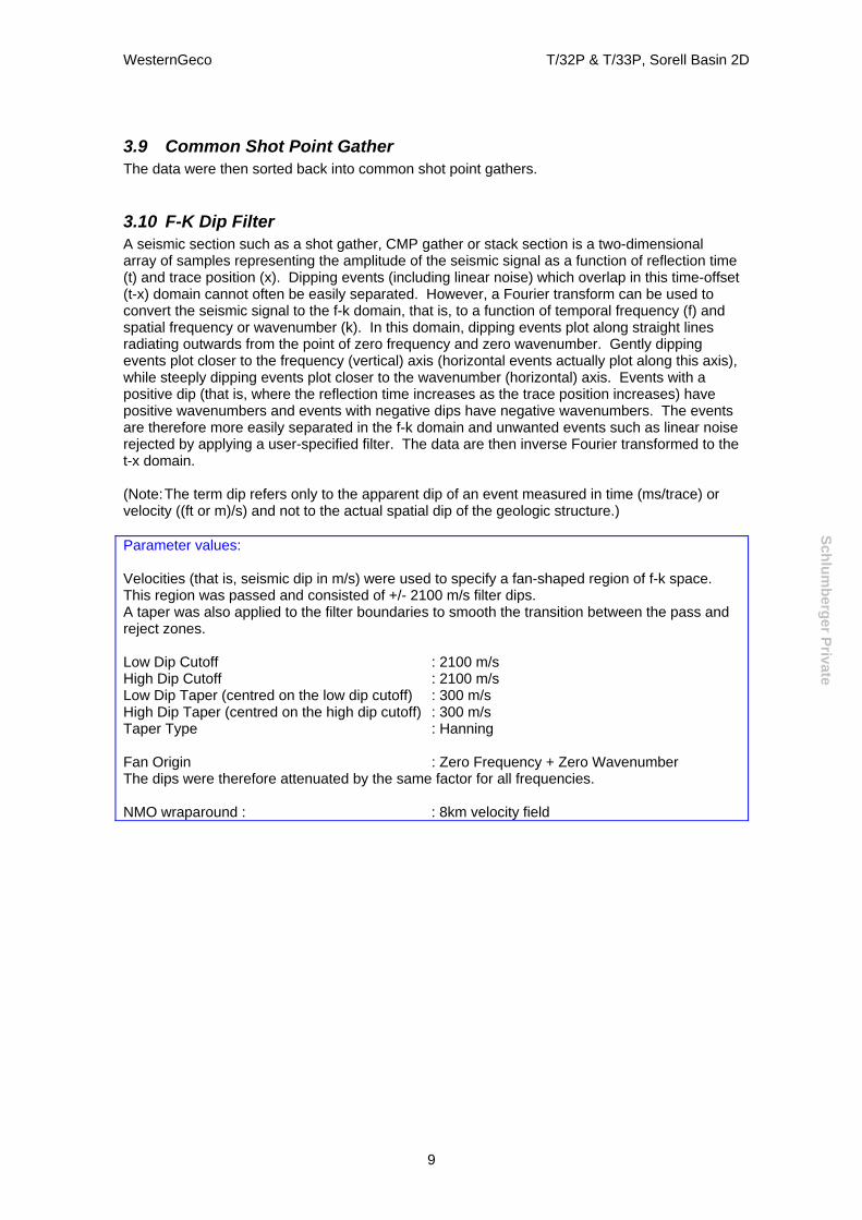
3.9 Common Shot Point Gather The data were then sorted back into common shot point gathers.

3.10 F-K Dip Filter A seismic section such as a shot gather, CMP gather or stack section is a two-dimensional array of samples representing the amplitude of the seismic signal as a function of reflection time (t) and trace position (x). Dipping events (including linear noise) which overlap in this time-offset (t-x) domain cannot often be easily separated. However, a Fourier transform can be used to convert the seismic signal to the f-k domain, that is, to a function of temporal frequency (f) and spatial frequency or wavenumber (k). In this domain, dipping events plot along straight lines radiating outwards from the point of zero frequency and zero wavenumber. Gently dipping events plot closer to the frequency (vertical) axis (horizontal events actually plot along this axis), while steeply dipping events plot closer to the wavenumber (horizontal) axis. Events with a positive dip (that is, where the reflection time increases as the trace position increases) have positive wavenumbers and events with negative dips have negative wavenumbers. The events are therefore more easily separated in the f-k domain and unwanted events such as linear noise rejected by applying a user-specified filter. The data are then inverse Fourier transformed to the t-x domain. (Note: The term dip refers only to the apparent dip of an event measured in time (ms/trace) or velocity ((ft or m)/s) and not to the actual spatial dip of the geologic structure.) Parameter values: Velocities (that is, seismic dip in m/s) were used to specify a fan-shaped region of f-k space. This region was passed and consisted of +/- 2100 m/s filter dips. A taper was also applied to the filter boundaries to smooth the transition between the pass and reject zones. Low Dip Cutoff : 2100 m/s High Dip Cutoff : 2100 m/s Low Dip Taper (centred on the low dip cutoff) : 300 m/s High Dip Taper (centred on the high dip cutoff) : 300 m/s Taper Type : Hanning Fan Origin : Zero Frequency + Zero Wavenumber The dips were therefore attenuated by the same factor for all frequencies. NMO wraparound : : 8km velocity field

9



Figure 3.10.1: FK spectrum of a single shot, no FK filtering applied, line SS02-11

Figure 3.10.2: FK spectrum of a single shot, FK filtering applied, line SS02-11

10



3.11 Resample An antialias filter was applied and the data were resampled. Parameter values: Input Trace Length : 10240ms Output Trace Length : 10240ms Input Sampling Interval : 2.0ms Output Sampling Interval : 4.0ms Antialias Filter: Phase : Minimum Cutoff Frequency : 93.75Hz Cutoff Slope : 36dB/oct

3.12 Prestack Shot Interpolation (2.5D) Input shot gathers are read and stored in the form of a cube where the x direction is receiver station number, the y direction is shot station number and the third direction is time. Interpolated shot gathers are then created by a ‘2.5 D’ interpolation. The cube of data is windowed in all 3 directions to create sub-volumes within which the interpolation takes place. These sub-volumes are overlapped to allow for blending of the interpolation results. This is done in order to conform to the premise of the algorithm that seismic events are linear or planar within each sub-volume. NMO is also applied prior to interpolation to further conform to this assumption In the ‘2.5 D’ method, interpolation is then only carried out in the shot (or common detector) direction, after Fourier transform to the f-x-ky domain. The operator used is then an average for all the receivers in the time-space window, which should produce more reliable operators than a simple 2D receiver domain interpolator. Parameter values: Input source spacing : 37.5m Output source spacing : 12.5m Time window length : 512ms Time overlap : 256ms Maximum dip : 40ms/tr Window width in the detector direction : 20 traces Window width in the source direction : 20 traces Window overlap in the detector direction : 6 traces Window overlap in the source direction : 6 traces The data was interpolated to decrease the trace spacing within the CMP gathers, to help avoid aliasing in the radon demulitple process. Without interpolation, the trace spacing within the CMP gathers would have been 75m. Interpolation decreased the trace spacing to 25m. The interpolated traces were removed after the radon demultiple process.

3.13 K-Filter / Trace Reduction A seismic section such as a shot gather, CMP gather or stack section is a two-dimensional array of samples representing the amplitude of the seismic signal as a function of reflection time (t) and trace position (x). A Fourier transform can be used to convert trace position to the spatial frequency or wavenumber (k) domain. A range of wavenumbers was specified to be

11



passed by the filter and a taper was also applied to the filter boundaries to smooth the transition between the pass and the reject regions. After k-filtering, the number of traces in each shot record was reduced by dropping alternate traces. Consequently, the k-filter was chosen to act as an anti-aliasing filter in the wavenumber domain, attenuating energy that would otherwise have become aliased when the trace separation was doubled by the dropping of alternate traces. Odd numbered traces were rejected, thus preserving the near trace position (at trace 576). For convenience, the k-filter was implemented in the f-k domain. A 2-D Fourier transform was used to convert trace position to the wavenumber domain and reflection time to the frequency (f) domain. After implementation of the k-filter the data were inverse Fourier transformed back to the t-x domain. Parameter values: Input Shot Records : 576 traces Output Shot Records : 288 traces High Wavenumber Cutoff : 0.5 of k-Nyquist (relative to input trace separation) Taper (centred on the high wavenumber cutoff) : 0.1 of k-Nyquist

3.14 Common Mid Point Gather The data were sorted into Common Mid Point (CMP) gathers.

3.15 2km Velocity Analysis A 2km velocity analysis was performed using the 8km first pass velocity function as the central function. Similarly to the first pass velocity analysis, the 2km velocity analysis were ftp’d to WesternGeco’s Adelaide office for Santos’ approval. To aid velocity picking, x and y co-ordinate information for each velocity location was loaded to IVP. This enables all the picks within a user-defined radius to be superimposed on the display. This is especially beneficial in areas where lines intersect, to ensure consistency in the velocity interpretation. The data input to the velocity analyses were processed through FK demultiple using 80% of the 8km velocity function and applied from water bottom x 1.5. Parameter Values: Analysis Spacing : 2km Number of CMPs per Analysis (MVF Stack) : 11 Number of CMPs per Analysis (Semblance Display) : 3 As part of the QC process, each line was stacked using the 2km velocity field prior to radon demultiple being applied. The stack sections were SEG-Y’d to CD and sent to Santos for their approval.

12



3.16 Radon Multiple Attenuation Radon Multiple Attenuation is principally a subtraction process. Unwanted coherent noise is isolated in the tau-p domain, inverse transformed to the x-t domain, and then subtracted from the original data. Multiple energy can be isolated in the tau-p domain because events with different velocities map to different parts of the domain. CMP gather data are first NMO corrected which means that the primary reflections are over corrected while the multiples are broadly flat or under corrected after the NMO. For convenience we refer to over corrected data as having negative dip (decreasing time with increasing offset), under corrected data has positive dip (increasing time with increasing offset) and 'flat' means no change in time with increasing offset. The data are then transformed into the tau-p domain by using either a parabolic, hyperbolic or linear radon transform. The range of p traces was chosen to cover at least the range of multiple energy to be removed. It is not necessary to include primary data in the transform, though its inclusion does no harm. As traces within a gather do not have offsets from zero to infinity a Geometry Compensation Filter must be applied. This filter is deterministic, i.e., based solely on the geometry of the input data, and is used to focus the energy in the tau-p domain. The geometry compensation filter can either be effected using the ‘least-squares approach’ which separately compensates each p-trace at each temporal frequency or by using ‘p-deconvolution’, a more simplified approach which computes and applies a separate filter at each temporal frequency but across the p-traces. To further refine the construction of the model of the multiple energy, parts of tau-p space representing primary energy were zeroed based on the knowledge that primary data is relatively flat and multiples are under corrected. Inverse tau-p transform and inverse NMO produces a model of the multiple energy. This was subtracted from the original data to produce the multiple attenuated output. Prior to the Radon transform a 300ms AGC scaling was applied to the data. This has the effect of reducing the impact on the transform of high amplitude events at near and far offsets. After the data were transformed back to the T-X domain the inverse of the scaling was applied, so essentially preserving relative amplitudes. Santos required the long offset data to be kept for future AVO work, so the demultiple was run in 2 passes, first to help remove some of the linear noise which was cutting across the long offset data and second to remove the multiple energy.

13



Parameter values: First Pass: NMO velocity : 2km velocity field Geometry Compensation Filter : p-deconvolution Number of p-traces used : 373 Maximum frequency : 93Hz Moveout type : Linear Multiple moveout range : 2000 to 4000ms Minimum moveout (i.e. for the first p-trace) : 2000ms Maximum moveout (i.e. for the last p-trace) : 4000ms Maximum reference offset : 7300m Minimum application time : 500ms Second Pass (as first pass except): Number of p-traces used : 420 Moveout type : Parabolic Multiple moveout range : -500 to 4000ms Minimum moveout (i.e. for the first p-trace) : 500ms Maximum moveout (i.e. for the last p-trace) : 4000ms Note: Moveouts used in making intermediate p-traces were linearly interpolated between the minimum and maximum moveouts. As part of the QC process, each line was stacked using the 2km velocity field. The stack sections were SEG-Y’d to DVD and sent to Santos for their approval.

Figure 3.16.1: CMP gathers, no radon applied, line SS02-27

14



Figure 3.16.2: CMP gathers, single pass of radon applied, line SS02-27

Figure 3.16.3: CMP gathers, 2 pass radon applied, line SS02-27

15



3.17 Data Reduction The interpolated traces were removed.

3.18 Marine 2D Geometry Nominal marine 2D geometry was assigned to the data. Parameter values: Shot interval : 37.5m Group interval : 25m CMP interval : 12.5m Num of traces / CMP Fold : 288 / 96 Near trace offset (trace 288) : variable, see Appendix 6.4

3.19 1km Velocity Analysis A third pass of velocity analysis at a 1km interval used the 2km velocity function as the centre function. As per the 2km analysis, x and y co-ordinate information for each velocity location was loaded to IVP to ensure consistency in the velocity interpretation. These velocity analyses were qc’d and approved by Bruce Hawkes of ECL at WesternGeco’s Perth office. Parameter Values for velocity analysis: Analysis Spacing : 1km Number of CMPs per Analysis (MVF Stack) : 11 Number of CMPs per Analysis (Semblance Display) : 3 The data input to the velocity analysis were processed through Kirchhoff prestack time migration utilising the following parameters: Parameter values for Kirchhoff pre-stack time migration: Traveltime computation : RTFM Aperture computation type : Ray Bending Max aperture time : 5100 ms Amplitude compensation mode : 2D Frequency limits : 0-125Hz Dip limit : 60 degrees

3.20 TVF A zero-phase TVF (Time Variant Filter) was applied to the data prior to KPSTM. The filter passbands were described by low- and high-cut frequencies and associated dB/octave cutoff slopes. The specified cutoff frequencies are located at the half-power (-3 dB in amplitude) response points and the slopes at these frequencies are equal to the respective dB/octave values. The slope is an approximate cosine squared function in the amplitude domain. The filters were normalized so that the output amplitudes were the same as the input amplitudes for frequency components within the passband.

16



Parameter values:

Filter Centre Time (ms)

Low-cut Frequency

(Hz)

Low-cut Slope (dB/octave)

High-cut Frequency

(Hz)

High-cut Slope (dB/octave)

Water bottom time (WB)

3 18 60 36

WB + 1000 3 18 50 36 WB + 2000 3 18 40 36 WB + 3000 3 18 30 36

Note: The times are those at the centre of the filter where the full effect of the filter is attained The first filter was applied from the beginning of the trace to the first filter centre time Intermediate filters were linearly tapered and blended with the preceding and succeeding filter between the filter centre times The last filter was applied from the last filter centre time to the end of the data

3.21 Kirchhoff Pre-Stack Time Migration In general, with increasing structural complexity, post-stack migration becomes less accurate, and the need for a pre-stack migration (PreSTM) arises. Pre-stack imaging becomes necessary where conflicting dips (or ‘stacking conflicts’) occur in the data, which results in inaccurate velocity analysis. The stacked section in this case is no longer being a good representation of a zero offset section Kirchhoff PreSTM has several benefits over the “common zero offset” approach which has been commonly used in recent years, primarily in it’s ability to improve structural imaging and provide correctly imaged pre-stack data for subsequent AVO analysis. Kirchhoff migration is a summation process, which is only performed for input traces that are within an aperture radius of the output point. The aperture radius is a time-variant function of the specified dip-limits. For each input trace and output sample, travel-times are computed to determine the proper input sample to sum. Input sample values are scaled and filtered before summing. Anti-alias filters as a function of dip and midpoint distance are applied to the data during migration. A V2T amplitude correction is effectively applied during the migration process, so any geometrical spreading correction applied should be removed prior to migration. The migration is run on common offset volumes, and as migrated velocities are required, it is run in an iterative fashion, giving improved velocity control with each pass. The iterative sequence is illustrated below, using as many passes as deemed necessary.

17



Kirchhoff PreSTM - Pass 1Using Preliminary Velocities

Output velocity lines every 2000m

Interpret and smooth velocity field

Kirchhoff PreSTM - Pass 2Using Pass 1 velocities

Output velocity lines every 1000m

Kirchhoff PreSTM - Final PassUsing Pass 3 velocities

Output all data

Interpret and smooth velocity field

Interpret velocity analyses at final required spacing

The migration was run using the 1km velocity field, smoothed over a 5km radius.

Parameter values: Traveltime computation : RTFM Aperture computation type : Ray Bending Max aperture time : 4000ms Amplitude compensation mode : 2D Number of offset planes : 96 Time variant frequency limits; Time (ms) Frequency (Hz)

0 90 4000 90 5000 75 6000 65 7000 55 10200 55

Time variant dip limits; Time (ms) Dip (degrees)

0 60 6000 60 10200 45

18



3.22 Geometric Spreading Amplitude Compensation Time-variant trace scaling functions were applied to the data to compensate for the decay in amplitude resulting from the propagation of a seismic wave from a point source in a layered medium. The functions were calculated from formulae based on the equation:

G(T) = V

2XT

V21

where V is the rms velocity associated with a reflection arriving at the two-way travel time, T, ssociated with shot-to-receiver offset, X.

1 (the first velocity in the velocity function) is used as a normalization factor.

he velocity and travel time information was varied spatially using the 1km velocity field.

C was carried out and approved by Bruce awkes of ECL at WesternGeco’s Perth office.

arameter Values for velocity analysis:

nalysis Spacing : 0.5km

umber of CMPs per Analysis (Semblance Display) : 3

a V T

3.23 Final 500M Velocity Analysis The final pass of velocity analysis was performed on a 500m interval using the 1km velocity functions as the center functions. As previously, the xy coordinates were loaded to ensure consistency in the velocity interpretation. The QH P A Number of CMPs per Analysis (MVF Stack) : 11N

MO corrections were applied using velocities from the final 500m velocity field.

veout adjust the reflection events to their zero offset equivalent using the following quation:

3.24 Normal Moveout N Normal moe

2

22

0 vxtt −=

w = travel time at off set x (m/s) here t

olute value of the source to detector offset distance (m)

v = moveout velocity (m/s)

0t = zero offset travel time (m/s) x = abs

19



3.25 Radon Multiple Attenuation A further pass of Radon Multiple Attenuation was applied to the KPSTM gathers prior to create the near and far angle stacks, and for the CMP gather archive. For more details on this process see section 3.16. Parameter values: NMO velocity : 500m velocity field Geometry Compensation Filter : least squares Number of p-traces used : 451 Maximum frequency : 90Hz Moveout type : Parabolic Multiple moveout range : -500 to 4000ms Minimum moveout (i.e. for the first p-trace) : 300ms Maximum moveout (i.e. for the last p-trace) : 2000ms Maximum reference offset : 7300m Minimum application time : 0ms Note: Moveouts used in making intermediate p-traces were linearly interpolated between the minimum and maximum moveouts.

3.26 CMP gather archive 2 sets of NMO corrected CMP gathers for all lines were archived in SEG-Y format to 3590E tapes. See Appendix 6.12 for the tape listing and Appendix 6.13.1 for the trace header byte location information.

3.27 Scaling (Instantaneous Gain) User-specified time windows were used to derive and apply scale factors to each data sample. These multipliers were calculated by centring the window over a sample, taking the average absolute amplitude of the window, defining a multiplier to make this average 0.9 times the desired output rms amplitude and applying it to the sample. The window centre was then moved down one sample and a new multiplier calculated and applied. In this way, multipliers were computed and applied to each sample from the first window application point to the last window application point. Parameter values: RMS Amplitude : 2000 Window length : Constant

Window Length (ms)

Start Time (ms)

End Time (ms)

500 Water Bottom 10240

Note: The times specified are the time of the first sample to be included in the first window and the time of the last sample to be included in the last window. The last multiplier calculated was applied constantly until the last live sample.

20



3.28 Mute

3.28.1 Inner Trace Mute A water bottom dependent inner trace mute was applied to the data in order to suppress multiple energy on the near offsets. To prevent a rapid amplitude change between the muted and live parts of the trace, a taper was applied from zero amplitude to full amplitude. This prevents distortion to the frequency spectrum of the stacked data, which would otherwise be introduced by an abrupt boundary. Parameter values: Taper Zone Length: 64 ms (prior to the mute times detailed below)

Source-to-Detector Offset m

Mute Time (ms)

For 100 < WB < 1000ms: 190 720 1540 1690

For 1000 < WB < 2000ms: 190 720 1540 1690

For 2000 < WB < 3000ms: 190 720 1540 1690

For 3000 < WB < 3500ms: 190 720 1540 1690

For 3500 =< WB : 190 720 1540

1500 2000 4000 10000

1500 2000 4000 10000

3500 4000 6000 10000

4500 6000 9000 10000

5250 7000 10000

Note: Mute times were linearly interpolated between the specified offsets.

3.28.2 Outer Trace Mute An outer trace mute (water bottom dependent) was applied to remove first break noise and any data which NMO had stretched beyond acceptable limits. To prevent a rapid amplitude change between the muted and live parts of the trace, a taper was applied from zero amplitude to full amplitude. This prevents distortion to the frequency spectrum of the stacked data, which would otherwise by introduced by an abrupt boundary. Parameter values: Taper Zone Length: 32 ms (prior to the mute times detailed below)

Source-to-Detector Offset (m)

Mute Time (ms)

For 50 < WB < 100ms: 216 290 350 425

40

100 300 600

21



1000 1975 3550 4975 7300

For 100 < WB < 150ms: 276

350 425 1000 1975 3550 4975

7300 For 150 < WB < 500ms:

326 390 475 1000 1975 3550 4975 7300

For 500 < WB < 1000ms: 601 675 975 1500 2775 4875 7275

For 1000 < WB < 1500ms: 1201 1500 2025 4350 7275

For 1500 < WB < 2500ms: 1851 2075 3050 7250

For 2500 < WB < 2700ms: 2376 3050 4250

7250 For 2700 < WB < 3000ms:

2466 2690 2990 3590 4190

7265 For 3000 < WB < 3500ms:

2591 2890 3340 4165

7315

960 1500 2499 3497 4502

70

300 600 960 1500 2499 3497 4502

150 300 460 960 1500 2499 3497 4502

505 599 999 1499 2501 3505 4695

965 1501 2496 3499 4494

1490 2499 3497 4531

2398 3499 4499 5343

2610 3001 3499 4000 4501 5418

3000 3500 4000 4701 5622

22



For 3500 < WB < 4000ms: 2741 3040 4240 7315

For WB >= 4000ms: 3040 4240 7315

3500 4000 5002 5900

4500 5502 6400

Note: Mute times were linearly interpolated between the specified offsets. Selected NMO corrected CMP gathers for each line were displayed for quality control, with both the inner and outer trace mute patterns overlaid on the display as a solid line.

3.29 Stack The traces within each gather were stacked to form a single output trace. The resultant trace is normalized sample by sample using the following function:

s(t) = 1

w(t)

The nominal CMP fold was 96 and the shot points were numbered at source positions.

3.30 Water Bottom Time Update The water bottoms were re-digitised on internal format QC display stacks generated after KPSTM and the values updated to the trace headers. An ascii file containing the digitised water bottom values was output, linearly interpolated and extrapolated for all CMP locations and updated to the migrated trace headers. Additionally, a mute was applied above these updated WB values to eliminate the migration swing. The water bottom times were converted to depth and stored for placement into the stack SEG-Y trace headers.

3.31 Navigation/Seismic data merge MCG supplied processed P190 navigation data. This was used to update the seismic trace header literals with the xy coordinates of the source positions. The navigation and seismic data sets were matched using line numbers and shot point numbers.

3.32 Data Archive The data was also stacked without application of the pre-stack scaling (section 3.27). These raw stack data sets were output to exabyte tape in SEG-Y format for archive. See Appendix 6.12 for details and Appendix 6.13.2 for byte header location information.

23



4.0 Post-Stack Seismic Data Processing

4.1 Tau-P Coherency Filter The Tau-P coherency filter is a digital time and space variant multichannel filter. It attenuates the random noise and enhances coherent signal within a range of specified dip angles. Parameter values: Panel width : 14 traces Minimum P value : -6ms/trc Maximum P value : +6ms/trc Minimum Semblance weighting :0.2 Maximum Semblance weighting :0.8

4.2 Trace mix An isotime weighted average of amplitudes over adjacent traces is output. As a result, the spatial coherency of flat events is enhanced. Parameter values: Width of weighting function : 5 traces Type of weighting function : Cosine Bell

The above two processes had a profoundly beneficial affect upon the signal to noise ratio, and is clearly illustrated by comparing the final filtered stack with that of the raw stack (see figures below).

Figure 4.2.1: No taup filtering applied, line SS02-05

24



Figure 4.2.2: Taup filtering applied, line SS02-05

4.3 TVF A zero-phase TVF (Time Variant Filter) was applied to the data. Parameter values:

Filter Centre Time (ms)

Low-cut Frequency

(Hz)

Low-cut Slope (dB/octave)

High-cut Frequency

(Hz)

High-cut Slope (dB/octave)

Water bottom time (WB)

10 18 70 36

WB + 500 10 18 70 36 WB + 2000 8 18 60 36 WB + 3000 6 18 40 36 WB + 4000 6 18 30 36

Note: The times are those at the centre of the filter where the full effect of the filter is attained The first filter was applied from the beginning of the trace to the first filter centre time Intermediate filters were linearly tapered and blended with the preceding and succeeding filter between the filter centre times The last filter was applied from the last filter centre time to the end of the data

25



4.4 Scaling (Cascaded Instantaneous Gain) The cascaded AGC gain consists of two passes of the gain algorithm. In the first pass, automatic gain control (AGC) was applied to the data. A gain computation zone of 1000ms was used. An average absolute amplitude is computed for the zone, and this value divided into the desired average amplitude (2000 RMS) gives a multiplier that is applied at the midpoint of the gain zone. The zone is then moved down the trace, one sample at a time and the computation repeated so that a multiplier is derived for each sample. From the centre of the first gain zone back to the start of data and from the centre of the last gain zone to the end of the trace, a constant value was applied. The second pass is the same as the first except that multipliers are computed only for amplitudes which are lower than the new reference averaged amplitude of 1500 RMS with a smaller computation window of 500ms. The longer 1000ms window was used to scale the overall section with time, whilst the 500ms window was used to compensate for ‘shadow’ below high amplitude reflectors. Parameter values: Type : Cascaded AGC Output RMS amplitude for window 1 / window 2 : 2000 / 1500 Window length for window 1/ window 2 : 1000ms / 500ms Window start time : Water bottom two-way time

4.5 CGM Files CGM files were created for the final filtered and scaled pre-stack migrated stack sections. All traces were displayed at a scale of 20tr/cm and 5cm/sec. The CGM files had a full side label with a location map, velocity boxes and intersections annotated. Shot point numbers were annotated at source position for all lines. A CD containing the CGM files was provided as a final product (see Appendix 6.12).

4.6 Data Archive The filtered and scaled migrated stack data were output to exabyte tape in SEG-Y format for archive. See Appendix 6.12 for details and Appendix 6.13.2 for byte header location information. For a listing of the SP and CMP relationships see Appendix 6.8.

4.7 Angle Stacks Angle stacks were created after radon demultiple had been applied to the kirchhoff pre-stack time migrated data (see section 3.25). No pre-stack scaling was applied to the angle stacks.

4.7.1 Near angle stack Near angle stacks were created by applying inner and outer trace mutes, hung from the water bottom. The inner trace mute was the same as that used for the production stack (see section 3.27.1). The outer trace mute was created by taking the midway function between 120% of the final outer trace mute and 100% of the final inner trace mute. See next page for graphical representation of these mutes.

4.7.2 Far angle stack Far angle stacks were created by applying inner and outer trace mutes, hung from the water bottom. The inner trace mute was taken from the mid way function between 120% of the final outer trace mute and 100% of the final inner trace mute i.e. the same as the outer trace mute used for the near angle stacks. The outer trace mute was 120% of the production outer trace mute. See next page for graphical representation of these mutes.

26



Figure 4.7.1: Graphical representation of mutes used for near and far angle stacks, SS02-11

For the near angle stacks the inner Mute is represented by the red line and the outer mute by the yellow line. For the far angle stacks, the inner mute is represented by the yellow line and the outer mute by the pink line.

4.8 Data Archive The near and far angle stacks were output to exabyte tape in SEG-Y format for archive. See Appendix 6.11 for details and Appendix 6.13.2 for byte header location information.

27



5.0 Personnel Key individuals involved in the project were: For Santos Limited: Stuart Brew Senior Staff Geophysicist Ric Smith Principal Geophysicist Bruce Hawkes ECL, Consultant for velocity QC For WesternGeco: Lawrence Cho Processing Manager Paul Tredgett Supervisor Richard Bisley Staff Geophysicist Alison Keighley Project Leader Kenneth Jayan Geophysicist Dated: …………………………… Signed: ……………………………………

28



6.0 Appendices

6.1 Survey Location Map

29



6.2 Survey Line Information

30



6.3 Acquisition Parameters General Vessel : MGC – R/V Polar Duke Location : Sorell Basin, Australia Date shot : December 2002 Recording Recording format : SEG-D 8058 REV.1 Record length : 10000 ms Sample rate : 2 ms Recording low-cut filter : Out 3Hz/6dB analog Recording high-cut filter : 206Hz @ 276 dB/Oct Nominal fold : 96 Streamer Number of streamers : 1 Group interval : 12.5 m Streamer length (active) : 7200 m Streamer depth : approx. 10 m Number of groups : 576 Near trace : 576 Near trace offset from source : 125m or 140 m Note : Refer to Appendix 6.4 for near trace offsets. Source Shotpoint interval : 37.5 m Array volume per source : 3500 cu in Source depth : 5 m Number of sub-arrays per source : 4 Navigation Header H0100SURVEY AREA Santos SS02 Sorell Basin, Australia H0101SURVEY DETAILS 2D Survey 7200m Streamer H0102VESSEL DETAILS vessel1 1 H0103SOURCE DETAILS Source 301 1 1 H0104STREAMER DETAILS Streamer 201 576 ch 1 1 H0105OTHER DETAILS Buoy 401 1 1 H0200SURVEY DATE 16/12/2002 H0201TAPE DATE Tuesday 17 December 2002 - 02:40am H0202TAPE VERSION UK00A P1/90 H0300CLIENT SANTOS H0400GEOPHYSICAL CONTRACTOR MGC ASA H0500POSITIONING CONTRACTOR FUGRO H0600POSITIONING PROCESSING MGC H0700POSITIONING SYSTEM Spectra H0800COORDINATE POSITION Centre of Source H0901OFFSET SYSTEM TO SOURCE 1 1 0.00 -130.50 H0902OFFSET SYSTEM TO STREAMER 1 1 0.00 -270.50 H0903OFFSET SYSTEM TO ANTENNA 1 1 -4.00 -17.60 H0904OFFSET SYSTEM TO ANTENNA 1 2 -5.60 -17.60 H0905OFFSET SYSTEM TO E/S 1 1 0.00 -10.50 H0906OFFSET SYSTEM TO E/S 1 2 0.00 -9.70 H1000CLOCK TIME 00:00 H1100RECEIVER GROUPS PER SHOT 576 H1400GEODETIC DATUM AS SURVEYED GDA-94 GRS-80 6378137.000 298.2572221 H1401DATUM SHIFT SURVEY TO WGS84 -0.0 -0.0 -0.0-0.000-0.000-0.000-0.0000000 H1500GEODETIC DATUM AS PLOTTED GDA-94 GRS-80 6378137.000 298.2572221 H1501DATUM SHIFT PLOT TO WGS84 -0.0 -0.0 -0.0-0.000-0.000-0.000-0.0000000 H1600DATUM SHIFT SURVEY TO PLOT 0.0 0.0 0.0 0.000 0.000 0.000 0.0000000

31



H1700VERTICAL DATUM Sea level Echosounder H1800PROJECTION TYPE 003 Transverse Mercator H2000GRID UNITS 1Metres 1.000000000000 H2001HEIGHT UNITS 1Metres 1.000000000000 H2002ANGULAR UNITS 1Degrees H2200LONGITUDE OF CM 141 0 0.000E H2301GRID ORIGIN (LAT, LON) 0 0 0.000N141 0 0.000E H2302GRID ORIGIN (E, N) 500000.00E10000000.00N H2401SCALE FACTOR 0.9996000000 H2402SCALE ORIGIN (LAT, LON) 0 0 0.000N141 0 0.000E H2600 WAYPOINT (E, N) 656010.05502873.0 H2600 WAYPOINT (E, N) 686342.65522259.5 H2600 Processed by SeisPos release 11.11

6.4 Near Trace Offsets

Line Number Near Trc offset SS02- (m)

1 140 2 140 3 140 4 140 5 140 6 140 7 140 8 140 9 140

10 140 11 140 12 140 13 140 14 125 15 140 16 125 17 140 19 140 21 140 23 140 25 140 27 140 29 125 31 125 33 125 35 125 37 125 39 125 41 125

32



6.5 Acquisition Line Listing Seq No. Line Name Direction FPSP LSP COMP/INC Comments

1 SS02-01-001 056° 1001 2065 Complete

14 SS02-02-014 331° 1660 897 Complete

2 SS02-03-002 239° 1999 897 Complete

15 SS02-04-015 152° 1001 2232 Complete

3 SS02-05-003 059° 1001 2137 Complete

13 SS02-06-013 153° 1001 1776 Complete

4 SS02-07-004 239° 1920 897 Complete FCSP 1920 d/t recording seis rec probs at SOL

12 SS02-08-012 333° 2447 897 Complete

5 SS02-09-005 059° 1001 2106 Complete

18 SS02-10-018 147° 1001 3153 Complete

6 SS02-11-006 239° 2020 1726 Incomplete Term Whales

7 SS02-11-007 239° 1725 1154 Incomplete Line aborted d/t air leak

8 SS02-11-008 239° 1167 897 Complete

19 SS02-12-019 328° 2882 897 Complete

9 SS02-13-009 059° 1001 2055 Complete Term Syntrak.LGSP 2030

33 SS02-14-033 151° 1001 1106 DNP Term - Whales

34 SS02-14-034 151° 1001 2004 Complete

10 SS02-15-010 238° 2342 897 Complete

32 SS02-16-032 328° 2123 897 Complete

11 SS02-17-011 059° 1001 2306 Complete

16 SS02-19-016 059° 1001 2188 Complete

17 SS02-21-017 238° 2100 897 Complete

20 SS02-23-020 238° 2240 897 Complete

21 SS02-25-021 058° 1001 2022 Incomplete Term, Syntrak Lockup

22 SS02-25-022 058° 2011 2289 Complete

23 SS02-27-023 239° 1844 1825 DNP Syntrak Lock at SOL

24 SS02-27-024 239° 1859 897 Complete

25 SS02-29-025 061° 1001 1984 Complete

26 SS02-31-026 242° 1904 897 Complete

27 SS02-33-027 064° 1001 1967 Complete

28 SS02-35-028 244° 1856 897 Complete

29 SS02-37-029 065° 1001 1949 Complete

30 SS02-39-030 245° 1850 897 Complete 31 SS02-41-031 066° 1001 1654 Complete

Total Km 1256.1

33



6.6 Final Processing Line Listing

Line Name FSP LSP Length Km SS02-01-001 1001 2065 39.94 SS02-02-014 1660 897 28.65 SS02-03-002 1999 897 41.36 SS02-04-015 1002 2232 46.16 SS02-05-003 1001 2137 42.64 SS02-06-013 1001 1776 29.10 SS02-07-004 1920 897 38.40 SS02-08-012 2447 897 58.16 SS02-09-005 1001 2106 41.48 SS02-10-018 1001 3153 80.74

SS02-11-006,7,8 2020 897 42.15 SS02-12-019 2882 897 74.48 SS02-13-009 1001 2030 38.63

SS02-14-033,34 1001 2004 37.65 SS02-15-010 2341 897 54.19 SS02-16-032 2123 897 46.01 SS02-17-011 1001 2306 48.98 SS02-19-016 1001 2188 44.55 SS02-21-017 2100 897 45.15 SS02-23-020 2240 897 50.40 SS02-25-021 1001 2289 48.34 SS02-27-023 1859 897 36.11 SS02-29-025 1001 1984 36.90 SS02-31-026 1904 897 37.80 SS02-33-027 1001 1967 36.26 SS02-35-028 1856 897 36.00 SS02-37-029 1001 1949 35.59 SS02-39-030 1850 897 35.78 SS02-41-031 1001 1654 24.53

Total Km 1256.1

6.7 Merged Line listing

Line Name. SEQ. DIR FSP LSP KMS SS02-11-006 6 239 2020 1726 11.06 SS02-11-007 7 239 1725 1168 20.93 SS02-11-008 8 239 1167 897 10.16 SS02-25-021 21 58 1001 2010 37.88 SS02-25-022 22 58 2011 2289 10.46

34



6.8 SP/CMP Relationships SP/CMP relationships for the final KPSTM stack SEG-Y datasets are as follows:

SP*100 (at source) SP RANGE SEG-Y LINE FCMP LCMP fsp lsp FSP LSP

SS02-01 1 3480 90333 206300 1001 2065 SS02-02 1 2577 175767 89900 1660 897 SS02-03 1 3594 209667 89900 1999 897 SS02-04 1 3978 90433 223000 1002 2232 SS02-05 1 3696 90333 213500 1001 2137 SS02-11 1 3657 211767 89900 2020 897 SS02-06 1 2613 90333 177400 1001 1776 SS02-07 1 3357 201767 89900 1920 897 SS02-08 1 4938 254467 89900 2447 897 SS02-09 1 3603 90333 210400 1001 2106 SS02-10 1 6744 90333 315100 1001 3153 SS02-11 1 3657 211767 89900 2020 897 SS02-12 1 6243 297967 89900 2882 897 SS02-13 1 3375 90333 202800 1001 2030 SS02-14 1 3297 90367 200233 1001 2004 SS02-15 1 4620 243867 89900 2341 897 SS02-16 1 3966 222033 89867 2123 897 SS02-17 1 4203 90333 230400 1001 2306 SS02-19 1 3849 90333 218600 1001 2188 SS02-25 1 4152 90333 228700 1001 2289 SS02-21 1 3897 219767 89900 2100 897 SS02-23 1 4317 233767 89900 2240 897 SS02-25 1 4152 90333 228700 1001 2289 SS02-27 1 3174 195667 89900 1859 897 SS02-29 1 3237 90367 198233 1001 1984 SS02-31 1 3309 200133 89867 1904 897 SS02-33 1 3186 90367 196533 1001 1967 SS02-35 1 3165 195333 89867 1856 897 SS02-37 1 3132 90367 194733 1001 1949 SS02-39 1 3147 194733 89867 1850 897 SS02-41 1 2247 90367 165233 1001 1654

35



6.9 Testing Log

6.9.1 Low Cut Filter Input: Conversion data, geometry and T^2 gain applied, every 106th shot for test line 11. Panel Comments Displays Produced Test No- No filter applied Shot gathers T01_01ar 1 3Hz low cut filter applied Shot gathers T01_02ar 2 4Hz low cut filter applied 3 5Hz low cut filter applied 4 6Hz low cut filter applied Decision: 3Hz 18dB/oct minimum phase low cut filter to be applied. Santos requirements were to keep as much bandwidth as possible and see what swatt could achieve after a 3Hz filter had been applied.

6.9.2 Initial Geometry test Input: Conversion data, geometry, field trace edits, gun and cable correction, 3Hz low cut filter and geometric spreading applied, for test lines 11, 16 and 19. Comments Displays Produced Test NoNo Mute applied CMP gathers T03_00cr - Shot gathers T03_00ar2 Alternate cmps Geometry stack T03_00dr This test was run to use as a base comparison without any processing applied.

6.9.3 Swatt Line 19 was chosen as the test line as it exhibited the most swell noise. Input: Conversion data, geometry, field trace edits, gun and cable correction, 3Hz low cut filter and geometric spreading. Tests were also run on lines 11 and 16 for confirmation that swatt was not affecting primary data. Comments Displays Produced Test No 1700m/s NMO wraparound, -400 stretch CMP gathers T03_18cr 1700m/s NMO wraparound,-400 stretch Shot gathers T03_18ar 1700m/s NMO wraparound,-400 stretch Swatt stack T03_18dr Difference display Shot gathers T03_18ahr Difference display Stack T03_18dhr Displays from T03_18 showed that some of the long offset primary data was being removed due to the stretch mutes. The tests were rerun using a stretch mute of –150: Comments Displays Produced Test No1700m/s NMO wraparound,-150 stretch Shot gathers T03_25ar Difference display, 1700m/s NMO wraparound, -150 stretch Shot gathers T03_25ahr Decision: Frequency 0-30Hz, Spatial width 21 traces, temporal gate 500ms, wraparound NMO using 1700 m/s constant velocity and -150 stretch limit.

36



6.9.4 Shot FK filter Input: Conversion data, geometry, field trace edits, gun and cable correction, 3Hz low cut filter, geometric spreading and swatt applied. NMO wraparound using the 8km picked velocity field was applied to all the shot FK filter tests. Testing was run on lines 11, 16 and 19. Comments Displays Produced Test No Stretch -400, Passing dips +/- 1900m/s. Shot gathers T04_05ar Stretch -400, Passing dips +/- 1900m/s. Cmp gathers T04_05cr Stretch -400, Passing dips +/- 1900m/s. Stack T04_05dr Difference display, above parameters Shot gathers T04_05ahr Difference display, above parameters Stack T04_05dhr Stretch -400, Passing dips +/- 1700m/s. Shot gathers T04_06ar Stretch -400, Passing dips +/- 1700m/s. Cmp gathers T04_06cr Stretch -400, Passing dips +/- 1700m/s. Stack T04_06dr Difference display, above parameters Shot gathers T04_06ahr Difference display, above parameters Stack T04_06dhr Difference display, swatt of passing dips of +/- 1900m/s and +/- 1700m/s Shot gathers T04_09ahr Difference display, swatt of passing dips of +/- 1900 m/s and +/- 1700m/s Stack T04_09dhr The following tests were run on lines 11 and 16 only. Comments Displays Produced Test No Stretch -400, Passing dips +/- 2100m/s. Shot gathers T04_14ar Stretch -400, Passing dips +/- 2100m/s. Cmp gathers T04_14cr Stretch -400, Passing dips +/- 2100m/s. Stack T04_14dr Difference display, above parameters Shot gathers T04_14ahr Difference display, above parameters Stack T04_14dhr Stretch -400, Passing dips +/- 2500m/s. Shot gathers T04_15ar Stretch -400, Passing dips +/- 2500m/s. Cmp gathers T04_15cr Stretch -400, Passing dips +/- 2500m/s. Stack T04_15dr Difference display, above parameters Shot gathers T04_15ahr Difference display, above parameters Stack T04_15dhr Stretch -150, Passing dips +/- 1900m/s. Shot gathers T04_17ar Stretch -150, Passing dips +/- 1900m/s. Cmp gathers T04_17cr Stretch -150, Passing dips +/- 1900m/s. Stack T04_17dr Difference display, above parameters Shot gathers T04_17ahr Difference display, above parameters Stack T04_17dhr Difference display, swatt of passing dips of +/- 1900m/s with –400 stretch and –150 stretch Shot gathers T04_18ahr Difference display, swatt of passing dips of +/- 1900m/s with –400 stretch and –150 stretch Stack T04_18dhr Decision: Pass dips of +/- 2100 m/s, taper of 300 ms/trace and NMO wraparound using the 8km velocity field and a -150 stretch limit.

6.9.5 FK spectrum Input: Conversion data, geometry, field trace edits, gun and cable correction, low cut filter, geometric spreading and NMO using the 8km picked velocity field applied. Testing ran on lines 11, 16, 19 and 27. Comments Displays Produced Test No Single shot CGM of FK spectrum T04_00_FKspec

37



Single shot with swatt and FK filter passing dips of –1900m/s CGM of FK spectrum T04_05_FKspec Single shot with swatt and FK filter passing dips of –1700m/s CGM of FK spectrum T04_06_FKspec Tests were run to QC the FK spectrum before and after the swatt and FK filter had been applied.

6.9.6 Designature/resample Statistical designature tests were run on line 11 using the production geometry data as input. The data was resampled to 4ms after statistical designature had been applied. Comments Display Test NoNo desig Shot gathers and amplitude spectrum T05_00 Desig, target wavelet 3-75Hz Shot gathers and amplitude spectrum T05_01 Desig, target wavelet 3-80Hz Shot gathers and amplitude spectrum T05_02 Desig, target wavelet 3-85Hz Shot gathers and amplitude spectrum T05_03 Desig, target wavelet 3-90Hz Shot gathers and amplitude spectrum T05_04 Desig, target wavelet 3-85Hz, Shot gathers and amplitude spectrum T05_05 Confirmation tests for the application of deterministic designature were carried out using a supplied far field signature. Santos required the output to be a zero phase. A 4ms resample was also tested after designature had been applied. These tests were run on lines 11 and 27: Comments Display Test NoSwatt/Fkfilter, no desig CMP gathers P0403_FKfilter_320th_cmp

Scaled stack P0403_FKfilter_scaled_stk Raw stack P0403_FKfilter_raw_stk Swatt/Fkfilter, desig, 2ms sample rate CMP gathers P0502_Desig_2ms_320th_cmp

Scaled stack P0502_Desig_2ms_scaled_stk Raw stack P0502_Desig_2ms_raw_stk Swatt/Fkfilter, desig, 4ms sample rate CMP gathers P0502_Desig_4ms_320th_cmp

Scaled stack P0502_Desig_4ms_scaled_stk Raw stack P0502_Desig_4ms_raw_stk Decision: Designature should not be applied, however the resample to 4ms should be applied after the FK filter.

6.9.7 Deconvolution before stack All DBS testing was run on line 11 and used a 2 window design and application. CMP gathers and a stack section with an autocorrelation were displayed for each test. Input data: conversion, geometry, field trace edits, gun/cable correction, 3Hz low cut filter, swatt, fK filter, deterministic designature (using supplied far field signature), geometric spreading and NMO applied. Comments Display Test NoNo deconvolution CMP gathers T10_00cr Scaled stack T10_00ds Deconvolution, 16ms gap, operator avg 7trc. CMP gathers T10_01cr Scaled stack T10_01ds Deconvolution, 24ms gap, operator avg 7trc. CMP gathers T10_02cr Scaled stack T10_02ds Deconvolution, 32ms gap, operator avg 7trc. CMP gathers T10_03cr Scaled stack T10_03ds Deconvolution, 48ms gap, operator avg 7trc. CMP gathers T10_04cr Scaled stack T10_04ds Deconvolution, 64ms gap, operator avg 7trc. CMP gathers T10_07cr Scaled stack T10_07ds

38



Deconvolution, 48ms gap, no operator avg. CMP gathers T10_05cr Scaled stack T10_05ds Deconvolution, 48ms gap, opr. avg whole gath. CMP gathers T10_06cr Scaled stack T10_06ds Deconvolution, 48ms gap, operator avg 7trc, with one design window. CMP gathers T10_08cr Scaled stack T10_08ds Decision: Deconvolution before stack will not be applied.

6.9.8 Shot Interpolation/CMP interleave/Intra-gather interpolation These tests were run on line 11 only, to demonstrate the need for a finer trace spacing within the CMP gathers in order to get better results from the radon demultiple. Input data: production swatt data, FK filter, 4ms resample and array forming (to produce a 12.5m CMP interval) applied, every 160th CMP. Comments Display Test NoNo radon applied CMP gathers T06_14cr_noradon Radon applied CMP gathers T06_14cr 3:1 intra-gather interp CMP gathers T06_13cr_intrp_noradon 3:1 intra-gather interp/radon CMP gathers T06_13cr_intrp 3:1 intra-gather interp/radon/reject interp trc CMP gathers T06_13cr 3 CMP interleave CMP gathers T06_11cr_intl_noradon 3 CMP interleave/radon CMP gathers T06_11cr_intl 3 CMP interleave/radon/uninterleave CMP gathers T06_11cr Input data: production swatt data, FK filter, 3:1 shot interpolation, 4ms resample and array forming (to produce a 12.5m CMP interval) applied, every 160th CMP. Comments Display Test NoNo radon applied CMP gathers T06_12cr_noradon Reject interp trc, no radon applied CMP gathers T06_12cr2_noradon Radon applied CMP gathers T06_12cr Radon applied, reject interp trc CMP gathers T06_12cr2 Radon demultiple was applied using the following parameters: NMO: using 100% 2km velocity field Method: least squares modelling Model parabolic moveout range: -500 to 4000ms Reject parabolic moveout range: 250 to 4000ms Reference offset: 7300m Velocity mutes: 20% - 98% No: p-traces: 576 Maximum frequency: 93Hz Decision: 3:1 shot interpolation to be applied prior to demultiple, to give a trace spacing within the CMP gathers of 25m (75m prior to interpolation).

6.9.9 Array forming/Kfilter, trace decimate The best method to create a 12.5 m CMP interval was tested on line 11. Input data: production swatt data, FK filter applied. Comments Display Test NoArray forming applied Shot gathers T07_00ar Kfilter/trace decimate applied Shot gathers T08_00ar A FK spectrum of a shot from each test was also produced. Decision: apply Kfilter and trace decimate to produce a 12.5m CMP interval prior to demultiple.

39



6.9.10 FK demultiple/Radon demultiple The fast track migration on Santos’ adjacent survey had FK demultiple applied, so Santos required a comparison test between FK and radon demultiple. Input data: production swatt data, FK filter, 3:1 shot interpolation and 4ms resample applied, every 320th CMP: Comments Display Test NoNo radon applied CMP gathers T06_12cr_noradon Reject interp trc, no radon applied CMP gathers T06_12cr2_noradon Radon applied CMP gathers T06_06cr Radon applied/reject interp trc CMP gathers T06_06cr2 FK demultiple applied CMP gathers T06_02cr FK demultiple applied/reject interp trc CMP gathers T06_02cr2 Radon demultiple was applied using the following parameters: NMO: using 100% 2km velocity field Method: least squares modelling Model parabolic moveout range: -500 to 4000ms Reject parabolic moveout range: 250 to 4000ms Reference offset: 7300m Velocity mutes: 20% - 98% No: p-traces: 576 Maximum frequency: 93Hz FK demultiple was applied using the following parameters: NMO: using 90% 2km velocity field Application window: WB*1.9 – tmax Multiple attenuation filter: Pass Negative zero Decision: Radon demultiple is to be applied.

6.9.11 Radon demultiple Radon demultiple was tested on lines 11 and 27. All test displays were of NMO corrected CMP gathers, NMO using the 2km picked velocity field. Input data: production swatt, FK filter, 3:1 shot interpolation, 4ms resample and kfilter/trace decimate applied. Comments Display Test NoNo radon applied CMP gather T06_17cr No radon applied / interp trc rejected CMP gather T06_17cr2 Radon 1 CMP gather T06_12cr Radon 1 / interp trc rejected CMP gather T06_12cr2 Radon 2 CMP gather T06_20cr Radon 2 / interp trc rejected CMP gather T06_20cr2 Radon 3 / Radon 2 CMP gather T06_24cr Radon 3 / Radon 2 / interp trc rejected CMP gather T06_24cr2 Radon 3 CMP gather T06_23cr Radon 1 parameters: NMO: using 100% 2km velocity field Method: least squares modelling Model parabolic moveout range: -500 to 4000ms Reject parabolic moveout range: 250 to 4000ms Reference offset: 7300m Velocity mutes: 20% - 98% No: p-traces: 576 Maximum frequency: 93Hz Radon 2 parameters: As per radon 1 parameters except: Reject parabolic moveout range: 500 to 4000ms

40



Radon 3 parameters: NMO: using 100% 2km velocity field Method: p-decon Model linear moveout range: 1000 to 4000ms Reject linear moveout range: 1000 to 4000ms Reference offset: 7300m No: p-traces: 576 Maximum frequency: 93Hz After Santos had QC’d the 2km velocity field, they felt that it had been picked too fast. The field was slowed down and the following confirmation tests were run: Comments Display Test No No radon CMP gather T06_64cr Scaled stack T06_64ds Radon4 / Radon5 CMP gather T06_65cr Scaled stack T06_65ds Radon 4 parameters: NMO: using 100% 2km velocity field Method: p-decon Model linear moveout range: 2000 to 4000ms Reject linear moveout range: 2000 to 4000ms Time range to form p-traces: 0 to 2500ms Reference offset: 7300m Maximum frequency: 93Hz Radon 5 parameters (as radon 4 except): Model parabolic moveout range: -500 to 4000ms Reject parabolic moveout range: 500 to 4000ms Velocity mutes: 20% - 95% Decision: 2 pass radon demultiple is to be applied using the parameters above (radon 4 and 5). Radon is only to be applied below 500ms in order to protect the shallow data.

6.9.12 Migration Tests were run on line 11 to compare the results of running Kirchhoff pre-stack time migration, DZO pre-stack time migration and a post-stack Kirchhoff migration. Input data: production FK filter data, radon demultiple and DBS applied. Comments Display Test NoDZO PSTM applied Migrated Stack T11_26es_40deg Kirchhoff PSTM applied Migrated Stack T13_16es DMO stack/post-stack Kirchhoff migration Migrated Stack T12_07es Decision: Kirchhoff pre-stack time migration to be applied, using a maximum dip of 60 degrees from 0-4500ms and 45 degrees from 6000ms. Confirmation testing of the Kirchhoff PSTM was done on line 27, as this line contained linear noise, was shot in shallow water and also contained a high amplitude residual multiple. Because of the complicated nature of the water bottom and the underlying structure, Santos thought that migrating the data with a 500m velocity field rather than the proposed 1km velocity field would give better results. This was tested on line 11. The velocity field was picked on a 500m grid after KPSTM had been applied and smoothed over a 5km radius. For the other test, this velocity field was first decimated to a 1km grid before being smoothed. Comments Display Test No500m velocity field CMP gathers T13_14cr Stack T13_14es 1km velocity field CMP gathers T13_15cr

41



Stack T13_15es Decision: Kirchhoff pre-stack time migration to be applied using the 1km velocity field, smoothed over 5km.

6.9.13 Hybrid Depth migration Due to the uneven nature of the water bottom, a hybrid depth migration test was conducted on line 10 to see if this method of migration stopped the data from sagging under the WB structures and compared to the Kirchhoff PSTM. Comments Display Test No Kirchhoff pre-stack time migration Stack T13_15es Hybrid pre-stack depth migration Stack T16_26es Decision: Hybrid depth migration is not to be applied.

6.9.14 Pre-migration noise reduction The following tests were run to try and reduce the migration artefacts caused by the high amplitude residual multiple on line 27. Input data: production FK filtered data, radon and DBS applied. Comments Display Test No1000ms AGC prior to KPSTM CMP gathers T13_19cr Stack T13_19es TVF prior to KPSTM CMP gathers T13_20cfr Stack T13_20efs TVF/Despike prior to KPSTM CMP gathers T13_21cfr Stack T13_21efs ZAP, no KPSM applied CMP gathers T19_01cr Decision: Apply TVF prior to Kirchhoff pre-stack time migration: Time (ms) Low cut High cut WB 3Hz,18dB/oct 60Hz 36dB/oct WB+1000 3Hz, 18dB/oct 50Hz, 36dB/oct WB+2000 3Hz, 18dB/oct 40Hz, 36dB/oct WB+3000 3Hz, 18dB/oct 30Hz, 36dB/oct

6.9.15 Radon demultiple (final pass) A final pass of radon demultiple using the final velocity field was tested on lines 5, 11 and 27. Input: Production KPSTM CMP gathers. Comments Display Test No No radon CMP gathers T22_11_KPSTM_SEGY_CMPS Radon applied CMP gathers T22_11_RADON2_SEGY_CMPS Radon parameters were as follows: NMO: using 100% 500m velocity field Method: least squares modelling Model parabolic moveout range: -500 to 2000ms Reject parabolic moveout range: 300 to 2000ms Reference offset: 7300m Maximum frequency: 93Hz Velocity mutes: 20% - 95% of 500m velocity field. Decision: A final pass of radon demultiple using the final 500m velocity field is to be applied to the KPSTM gathers for archive and also to the near and far angle stacks. It is not necessary to apply it to the final stack dataset.

42



6.9.16 Prestack Scaling Pre-stack scaling tests were run on line 5. Input: production KPSTM gathers. Tau P filter, TVF and cascaded AGC were applied post stack. Comments Display Test No No pre stack scaling CMP gathers T25_15ecr

Stack T25_15eds Pre-stack AGC of 1000ms window length CMP gathers T25_16ecr Stack T25_16eds Pre-stack AGC of 500ms window length CMP gathers T25_17ecr

Stack T25_17eds Pre-stack Trace balance CMP gathers T25_18ecr

Stack T25_18eds Decision: Apply pre-stack scaling with 500ms window length to the final filtered stack.

6.9.17 Near and Far angle mutes Mute tests were run on line 5. Percentages of outer traces mutes (OTM) and inner traces mutes (ITM) were created and applied to a series of KPSTM stacks to help optimise the near and far angle mutes. Input: Production KPSTM gathers. TauP filter, TVF and AGC were applied post-stack. Comments Display Test No100% OTM and 100% ITM Stack T17_13_KPSTMSTK_100_OTM_100_ITM 100% OTM and 150% ITM Stack T17_13_KPSTMSTK_100_OTM_150_ITM 100% OTM and 50% ITM Stack T17_13_KPSTMSTK_100_OTM_50_ITM 110% OTM and 100% ITM Stack T17_13_KPSTMSTK_110_OTM_100_ITM 120% OTM and 100% ITM Stack T17_13_KPSTMSTK_120_OTM_100_ITM 80% OTM and 100% ITM Stack T17_13_KPSTMSTK_80_OTM_100_ITM 90% OTM and 100% ITM Stack T17_13_KPSTMSTK_90_OTM_100_ITM All mutes graphed only CMP gathers T17_14cr_KPSTM_MUTES Decisions: The 100% OTM and 100% ITM are to be applied to the final stack. The near angle stacks are to use 100% ITM and the midway function between 100% ITM and 120% OTM as the outer trace mute. The far angle stacks are to use the near angle outer mute as the inner mute and 120% OTM as the outer trace mute.

6.9.18 Post stack Noise Reduction Noise reduction tests were run on line 5. Input: production KPSTM stack data. Comments Display Test No No filter applied Stack T26_06efs Dip filter +/- 4ms/tr Stack T26_10efs RPF, 5 traces, fan +/- 5ms/tr Stack T23_06efs TauP, +/- 6 P traces, Min semb 0.2, Max semb 0.8 Stack T24_14efs Tracemix, 11 traces Stack T29_05efs Decision: Apply TauP filter (+/- 6 ms/tr) followed by a trace mix using 5 traces.

43



6.9.19 Post stack Time Variant Filter (TVF) Post stack filter tests were run on line 5. Input: production KPSTM stack data. Comments Display Test NoKPSTM- no filter Stack T28_00eds Low cut 6Hz, High cut 20Hz Stack T28_01edf Low cut 21Hz, High cut 30Hz Stack T28_02edf Low cut 31Hz, High cut 40 Hz Stack T28_03edf Low cut 41Hz, High cut 50 Hz Stack T28_04edf Low cut 51Hz, High cut 60 Hz Stack T28_05edf Low cut 61Hz, High cut 70 Hz Stack T28_06edf Low cut 71Hz, High cut 80 Hz Stack T28_07edf Low cut 6Hz, High cut 20Hz Stack T28_09edf Low cut 6Hz, High cut 30Hz Stack T28_10edf Low cut 6Hz, High cut 40 Hz Stack T28_11edf Low cut 6Hz, High cut 50 Hz Stack T28_12edf Low cut 6Hz, High cut 60 Hz Stack T28_13edf Low cut 6Hz, High cut 70 Hz Stack T28_14edf Low cut 6Hz, High cut 80 Hz Stack T28_15edf Low cut 4Hz, High cut 60Hz Stack T28_16edf Low cut 6Hz, High cut 60Hz Stack T28_17edf Low cut 8Hz, High cut 60 Hz Stack T28_18edf Low cut 10Hz, High cut 60 Hz Stack T28_19edf Low cut 12Hz, High cut 60 Hz Stack T28_20edf Low cut 14Hz, High cut 60 Hz Stack T28_21edf Decision: Apply the following final post-stack TVF: Filter Time Low-cut filter High-cut filter WB 10Hz, 18dB/oct 70Hz, 36dB/oct WB + 500ms 10Hz, 18dB/oct 70Hz,36dB/oct WB + 2000ms 8Hz, 18dB/oct 60Hz,36dB/oct WB + 3000ms 6Hz, 18dB/oct 40Hz,36dB/oct WB + 4000ms 6Hz, 18dB/oct 30Hz,36dB/oct

6.9.20 Post stack scaling Scaling tests were run on line 5. Input: production KPSTM stack data. Comments Display Test No500ms AGC Stack T30_02efs 1000ms AGC Stack T30_04efs 1500ms AGC Stack T30_05efs Cascaded AGC: Win1: 1000ms, Win2: 250ms Stack T30_09efs Cascaded AGC: Win1: 1000ms, Win2: 500ms Stack T30_10efs Cascaded AGC: Win1: 500ms, Win2: 250ms Stack T30_13efs Cascaded AGC: Win1: 750ms, Win2: 250ms Stack T30_14efs Cascaded AGC: Win1: 1500ms, Win2: 250ms Stack T30_15efs Decision: Apply cascaded AGC with window length 1: 1000ms and window length 2: 500ms.

44



6.10 Data Processing Flowchart SEG-D Conversion

Field trace edits

Nominal Geometry UpdateShot/Group/CMP interval:

37.5m/12.5m/6.25m

Gun and cable correction

Low Cut filter3Hz 18 dB/oct

Swell noise attenuationNMO wraparound 1700m/s, freq 0-30Hz, 21 trace filter width

500ms gate length applied in receiver domain

Shot FK filterNMO wraparound 8km vels, pass velocity dips

+/- 2100 m/s, taper 300 m/s.

Time Resample to 4msMin phase antialias filter 93Hz, 36 db/oct

Shot InterpolationOutput 12.5m shot spacing

K Filter / trace decimate+/- 0.5 K cut / odd traces

rejected

Inverse NMO

Preliminary 8kmVelocity analysis

2km Velocity analysis

FK Demultipleapplied to velocity data

2 Pass Radon Demultiple1st pass: model & reject linear moveout range

2000-4000ms, 373 p-trc.2nd pass: model parabolic moveout -500-4000ms,

reject 500-400ms, 420 p-trc.

Interpolated traces rejectedKPSTMapplied to velocity data

SEG Youtput

to 3590

NMO

NMOInterpolated

traces rejected

QC stacks

QC stacks

StackSEG Youtputto CD

StackSEG Youtputto CD

45



1km Velocity analysisKirchhoff Pre-Stack Time Migration

Max dip/time 60o/0-6sec; 45o,/10 sec.Max aperture time 4sec, dist 4km.

Time Variant Fiter

Amplitude CompensationGeo. spreading using 1 km vels.

Final 500m Velocityanalysis

NMOFinal 500m velocity

Final500m

velocitiesVelf text to

CD

Inner and Outertrace mutes

Stack

Raw stackSEG Y output

to exabyte

Scaling500ms AGC

Tau-P filterMin/max P values +/-6ms/tr, semb 0.2-0.85 Trace mix applied.

Time Variant Filter

ScalingCascaded AGC

Win 1 length 1000ms,Win 2 length 500ms

Final StackSEG Y output

to exabyte

Radon Demultiplemodel parabolic moveout-500-2000ms, reject 300-

2000ms, 307 p-trc.

Raw gathersSEG Y

output to3590

Near angle stack


Time Variant Filter

ScalingCascaded AGC


NearAngleStack

SEG Youtput toexabyte

RawNearAngle

StackSEG Y

output toexabyte

Far angle stack


Time Variant Filter

ScalingCascaded AGC


Far AngleStackSEG Y

output toexabyte

Raw FarAngle Stack

SEG Youtput toexabyte

Stack

46



6.11 Example displays at various processing stages

6.11.1 Line: SS02-05

Figure 6.11.1.1: QC stack, no radon demultiple applied, stacked using 2km velocity field.

Figure 6.11.1.2: QC stack, radon demultiple applied, stacked using 2km velocity field.

47



Figure 6.11.1.3: QC migrated stack, KPSTM applied, stacked using 1km velocity field.

Figure 6.11.1.4: Filtered migrated stack, KPSTM and post stack processing applied.

48



6.11.2 Line: SS02-27

Figure 6.11.2.1: QC stack, no radon demultiple applied, stacked using 2km velocity field.

Figure 6.11.2.2: QC stack, radon demultiple applied, stacked using 2km velocity field.

49



Figure 6.11.2.3: QC migrated stack, KPSTM applied, stacked using 1km velocity field.

Figure 6.11.2.4: Filtered migrated stack, KPSTM and post stack processing applied.

50



6.12 Tape Disposition Data Permit Media Copies Tape Nos. Date Sent Demultiple stacks T/32P,T/33P DVD 1 OP000464 29/05/2003 (hand carried) Final filtered stacks T/32P,T/33P Exabyte 2 X00828 15/08/2003 X00834 15/08/2003 T/32P Exabyte 1 X00829 15/08/2003 T/33P Exabyte 1 X00830 15/08/2003 Filtered near angle stks T/32P,T/33P Exabyte 2 X00831 15/08/2003 X00835 15/08/2003 T/32P Exabyte 1 X00832 15/08/2003 T/33P Exabyte 1 X00833 15/08/2003 Filtered far angle stks T/32P,T/33P Exabyte 2 X00836 15/08/2003 X00842 15/08/2003 T/32P Exabyte 1 X00837 15/08/2003 T/33P Exabyte 1 X00854 15/08/2003 Raw filtered stacks T/32P,T/33P Exabyte 2 X00838 15/08/2003 X00843 15/08/2003 T/32P Exabyte 1 X00839 15/08/2003 T/33P Exabyte 1 X00841 15/08/2003 Raw near angle stks T/32P,T/33P Exabyte 2 X00838 15/08/2003 X00843 15/08/2003 T/32P Exabyte 1 X00839 15/08/2003 T/33P Exabyte 1 X00841 15/08/2003 Raw far angle stks T/32P,T/33P Exabyte 2 X00844 15/08/2003 X00848 15/08/2003 T/32P Exabyte 1 X00845 15/08/2003 T/33P Exabyte 1 X00853 15/08/2003 Velocity field T/32P,T/33P CD 1 OP000594 CD-R1 15/08/2003 T/32P CD 1 OP000594 CD-R2 15/08/2003 T/33P CD 1 OP000594 CD-R3 15/08/2003 Radon PSTM Gathers T/32P,T/33P 3590E 2 Q50870-Q50898 15/08/2003 Q50900-Q50928 15/08/2003 Final report T32/P,T/33P CD 3 CD-Report1a 13/10/2003 CD-Report1b 13/10/2003 CD-Report1c 13/10/2003 T/32P CD 1 CD-Report2 13/10/2003 T/33P CD 1 CD-Report3 13/10/2003 CGMs T/32P,T/33P CD 1 CD-CGM1 02/10/2003

51



6.13 SEG-Y Trace Header Byte Locations

6.13.1 KPSTM CMP Gathers DATA_TYPE Starting BYTE Description 'INTEGER' 17 'CMP' 'INTEGER' 21 'CMP' ‘HALFWORD' 33 'STACK WORD' 'INTEGER' 61 'WATER DEPTH Midpoint' 'INTEGER' 65 'WATER DEPTH Midpoint' 'INTEGER' 73 'XCORD Midpoint' 'INTEGER' 77 'YCORD Midpoint' 'INTEGER' 81 'XCORD Midpoint' 'INTEGER' 85 'YCORD Midpoint' 'HALFWORD' 91 'Water Velocity' 'HALFWORD' 99 'Source Correction' 'HALFWORD' 101 'Cable Correction' 'HALFWORD' 103 'Total Gun and Cable Correction (Microsec)' 'INTEGER' 125 'XCORD Midpoint' 'INTEGER' 129 'YCORD Midpoint' 'HALFWORD' 141 'Anti Alias Filter * 100 (Hz)' 'HALFWORD' 143 'Anti Alias Filter Slope (db/oct)' 'HALFWORD' 149 'Low Cut Frequency (Hz)' 'HALFWORD' 151 'High Cut Frequency (Hz)' 'HALFWORD' 153 'Low Cut Filter Slope (db/oct)' 'HALFWORD' 155 'High Cut Filter Slope (db/oct)' 'HALFWORD' 157 'Year data recorded' 'HALFWORD' 159 'Julian day of the Year' 'INTEGER' 181 'XCORD Midpoint' 'INTEGER' 185 'YCORD Midpoint' 'INTEGER' 189 'CMP' 'INTEGER' 193 'CMP' 'INTEGER' 213 'WATER DEPTH Midpoint' 'INTEGER' 217 'CMP' 'INTEGER' 233 'Line Number'

6.13.2 Stack DATA_TYPE Starting BYTE Description 'INTEGER' 17 'Shotpoint Number' 'INTEGER' 21 'CMP' 'HALFWORD' 33 'STACK WORD' 'INTEGER' 61 'WATER DEPTH Midpoint' 'INTEGER' 65 'WATER DEPTH Midpoint' 'INTEGER' 73 'XCORD Midpoint' 'INTEGER' 77 'YCORD Midpoint' 'INTEGER' 81 'XCORD Midpoint' 'INTEGER' 85 'YCORD Midpoint' 'HALFWORD' 91 'Water Velocity' 'HALFWORD' 99 'Source Correction' 'HALFWORD' 101 'Cable Correction' 'HALFWORD' 103 'Total Gun and Cable Correction (Microsec)' 'INTEGER' 125 'XCORD Midpoint' 'INTEGER' 129 'YCORD Midpoint' 'HALFWORD' 141 'Anti Alias Filter * 100 (Hz)' 'HALFWORD' 143 ‘Anti Alias Filter Slope (db/oct)' 'HALFWORD' 149 'Low Cut Frequency (Hz)' 'HALFWORD' 151 'High Cut Frequency (Hz)' 'HALFWORD' 153 'Low Cut Filter Slope (db/oct)' 'HALFWORD' 155 'High Cut Filter Slope (db/oct)' 'HALFWORD' 157 'Year data recorded' 'HALFWORD' 159 'Julian day of the Year' 'HALFWORD' 167 'Time code 1 = Local' 'INTEGER' 181 'XCORD Midpoint' 'INTEGER' 185 'YCORD Midpoint' 'INTEGER' 189 'Shotpoint Number' 'INTEGER' 193 'CMP' 'INTEGER' 213 'WATER DEPTH Midpoint' 'INTEGER' 217 'CMP' 'INTEGER' 233 'Line Number'

52

Documents

Data Processing Report - Mineral Resources Tasmania · 2018-05-11 · WesternGeco T/32P & T/33P, Sorell Basin 2D S c h l u m b e r g e r P r i v a t e 1.0 Introduction This report