Data Processing & Calibrations

TM-H14-LIN

\

Sensit Inc

1652 Plum Ln. Suite 106

Redlands, CA 92374

http://www.sensit.com

Email: info@sensit.com

Paul 22apr13

3

Contents

Contents Processing Sensit Field Data - Introduction ............................................................................ 4

Model H14-LIN ........................................................................................................................ 4

About the new Model H14-LIN ................................................................................................ 4

Model H14-LIN improvements ................................................................................................ 5

Sensit PHA data requires pulse height analyzer .................................................................... 6

Generic PHA instrument structure .......................................................................................... 6

Sensit PHA data ...................................................................................................................... 6

Gain Selection ......................................................................................................................... 6

Model H14-LIN Wiring Color Code ......................................................................................... 7

Examples of possible circuits to control gain via data logger. ................................................ 8

Excellent Sand Catchers ......................................................................................................... 9

The BSNE catcher .................................................................................................................. 9

The Cox Sand Catcher ........................................................................................................... 9

Response .............................................................................................................................. 11

Threshold velocity ................................................................................................................. 11

Background ........................................................................................................................... 13

Drop Tube Test Results (Early calibration method) .............................................................. 13

New Model H14-LIN Radial Symmetry Lab Test .................................................................. 15

Sensor – Theory of operation ............................................................................................... 19

Instrument Calibration Constants (Lab & Field) .................................................................... 20

Laboratory Drop Tube Cal .................................................................................................... 21

Field Cal (Simplified) ............................................................................................................. 21

Simplified field data processing ............................................................................................ 24

Examples of Cal Method ........................................................................................................... 24

Particle Velocity .................................................................................................................... 25

Data Processing .................................................................................................................... 26

Paul 22apr13

4

Processing Sensit Field Data - Introduction

The basic field saltation data site is comprised of meteorological data towers complimented by

sand catchers and the Sensit wind eroding mass flux sensor. This paper provides a brief

background and suggested methods of processing Sensit field data.

The Sensit eroding mass sensor requires no maintenance and can operates nicely in a solar

powered remote erosion monitoring station. The data acquired provides estimates of mass flux

with high-resolution detail of erosion processes. The wind speed required to start movement on

the surface is easily determined shown in the particle impact (PC) data and is affectionately

referred to as the “threshold” of movement

Sand catchers should be checked daily, samples collected, weighted and collection time

recorded. Catcher mass (a total mass for the event reference) is necessary as a reference for

the processing of Sensit kinetic energy (KE) data collected for an erosion event. Accurate

catcher collection mass, data and time are very important values.

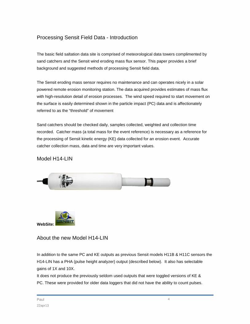
Model H14-LIN

WebSite:

About the new Model H14-LIN

In addition to the same PC and KE outputs as previous Sensit models H11B & H11C sensors the

H14-LIN has a PHA (pulse height analyzer) output (described below). It also has selectable

gains of 1X and 10X.

It does not produce the previously seldom used outputs that were toggled versions of KE &

PC. These were provided for older data loggers that did not have the ability to count pulses.

Paul 22apr13

5

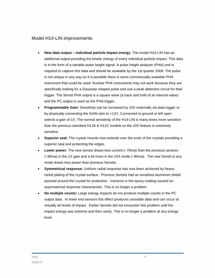
Model H14-LIN improvements

• New data output – individual particle impact energy: The model H14-LIN has an

additional output providing the kinetic energy of every individual particle impact. This data

is in the form of a variable pulse height signal. A pulse height analyzer (PHA) unit is

required to capture this data and should be available by the 1st quarter 2008. The pulse

is not unique in any way so it is possible there is some commercially available PHA

instrument that could be used. Nuclear PHA instruments may not work because they are

specifically looking for a Gaussian shaped pulse and use a peak detection circuit for their

trigger. The Sensit PHA output is a square wave (a track and hold of an internal value)

and the PC output is used as the PHA trigger.

• Programmable Gain: Sensitivity can be increased by 10X externally via data logger or

by physically connecting the GAIN wire to +12V. Connected to ground or left open

selects a gain of 1X. The normal sensitivity of the H14-LIN is many times more sensitive

than the previous standard H11B & H11C models so the 10X feature is extremely

sensitive.

• Superior seal: The crystal mounts now extends over the ends of the crystals providing a

superior seal and protecting the edges.

• Lower power: The new sensor draws less current (~70ma) than the previous sensors

(~90ma) in the 1X gain and a bit more in the 10X mode (~80ma). The new Sensit in any

mode draws less power than previous Sensits.

• Symmetrical response: Uniform radial response has now been achieved by heavy

nickel plating of the crystal surface. Previous Sensits had an anodized aluminum shield

epoxied around the crystal for protection. Variance in the epoxy coating caused an

asymmetrical response characteristic. This is no longer a problem.

• No multiple counts: Large energy impacts do not produce multiple counts in the PC

output data. In lower end sensors this effect produces unusable data and can occur at

virtually all levels of impact. Earlier Sensits did not encounter this problem until the

impact energy was extreme and then rarely. This is no longer a problem at any energy

level.

Paul 22apr13

6

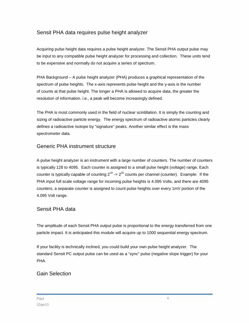
Sensit PHA data requires pulse height analyzer

Acquiring pulse height data requires a pulse height analyzer. The Sensit PHA output pulse may

be input to any compatible pulse height analyzer for processing and collection. These units tend

to be expensive and normally do not acquire a series of spectrum.

PHA Background – A pulse height analyzer (PHA) produces a graphical representation of the

spectrum of pulse heights. The x-axis represents pulse height and the y-axis is the number

of counts at that pulse height. The longer a PHA is allowed to acquire data, the greater the

resolution of information. i.e., a peak will become increasingly defined.

The PHA is most commonly used in the field of nuclear scintillation. It is simply the counting and

sizing of radioactive particle energy. The energy spectrum of radioactive atomic particles clearly

defines a radioactive isotope by "signature" peaks. Another similar effect is the mass

spectrometer data.

Generic PHA instrument structure

A pulse height analyzer is an instrument with a large number of counters. The number of counters

is typically 128 to 4095. Each counter is assigned to a small pulse height (voltage) range. Each

counter is typically capable of counting 216 -> 220

Sensit PHA data

counts per channel (counter). Example: If the

PHA input full scale voltage range for incoming pulse heights is 4.095 Volts, and there are 4095

counters, a separate counter is assigned to count pulse heights over every 1mV portion of the

4.095 Volt range.

The amplitude of each Sensit PHA output pulse is proportional to the energy transferred from one

particle impact. It is anticipated this module will acquire up to 1000 sequential energy spectrum.

If your facility is technically inclined, you could build your own pulse height analyzer. The

standard Sensit PC output pulse can be used as a “sync” pulse (negative slope trigger) for your

PHA.

Gain Selection

Paul 22apr13

7

Sensitivity can be increased by 10X externally via data logger or by physically connecting the

GAIN wire to +12V. Connected to ground or left open selects a gain of 1X. The dynamic range of

the pulse height output covers fine to medium size particle impact energies. The total dynamic

range (105

) of possible eroding particle energies is too great to be covered by a single linear A/D

system so we incorporated the selectable gain (X1, X10) to increase the PHA range capability.

Model H14-LIN eroding mass sensor

• Base diameter: 2.050”, length: 8.00” +/- 0.250”

• Upper post diameter: 1.050” length: 5.50” +/- 0.50”

• Crystal diameter: 0.915” length: 0.475” +/- 0.20”

• Top of base to center of crystal: length: 3.100” +/- 0.050

• Cable diameter: 0.210” length: 25 feet.

Outputs:

• Particle count (PC) data output is a CMOS/TTL compatible pulse indicating one particle impact,

• Kinetic energy (KE) is a CMOS/TTL compatible pulse representing a fixed amount of energy that has impacted the sensor. Each pulse represents the same amount of total energy and is calibrated by normalizing to the mass caught by a field catcher. The catcher mass normalization method compensates for a multitude of variables including day to day environmental effects of rain, humidity, radiation etc.

• NEW: Pulse height analysis (PHA) output is a pulse varying in amplitude with individual particle impacting energy. Pulse width: ~50uS, amplitude: 0 -> 5V. When input to a pulse height analyzer the PC output can be used as the sync if required.

Inputs:

• Power: +12VDC@70ma • Gain select (1X, 10X) can be selected via data logger output (open collector w/<10K pull

up resistor). Gain may also be selected by connecting this wire to ground (1X) or connected to +12V (10X).

Model H14-LIN Wiring Color Code Outputs

• (brown) KE (kinetic energy / pseudo mass flux) - CMOS/TTL compatible pulse

Paul 22apr13

8

• (white) PC (particle counts) - CMOS/TTL compatible pulse • (blue) PHA (particle energy) - variable pulse height

Input

• (green) GAIN – Ground (1X), +12VDC (10X). For data logger control use one of the circuits shown below

Power

• (red) Power + 12VDC @ 70ma • (black) Ground

Examples of possible circuits to control gain via data logger. Earlier models - H11B or C

(Replaced by Model H14-LIN)

Outputs

(brown) KE (mass) - pulse

(white) PC (particle counts) - pulse

Alternate outputs (seldom used)

(green) KE (mass) - variable pulse width

(blue) PC (particle counts) -variable pulse width

Power

(red) Power + 12VDC @ 90ma

(black) Ground

47K

1M

+12V

Sensit(Gain)

Data LoggerGeneral purposeTTL/CMOS output

Any NPNtransistor

Data LoggerGeneral purpose

Open collector outputSensit(Gain)

10K

10K

+12V

Paul 22apr13

9

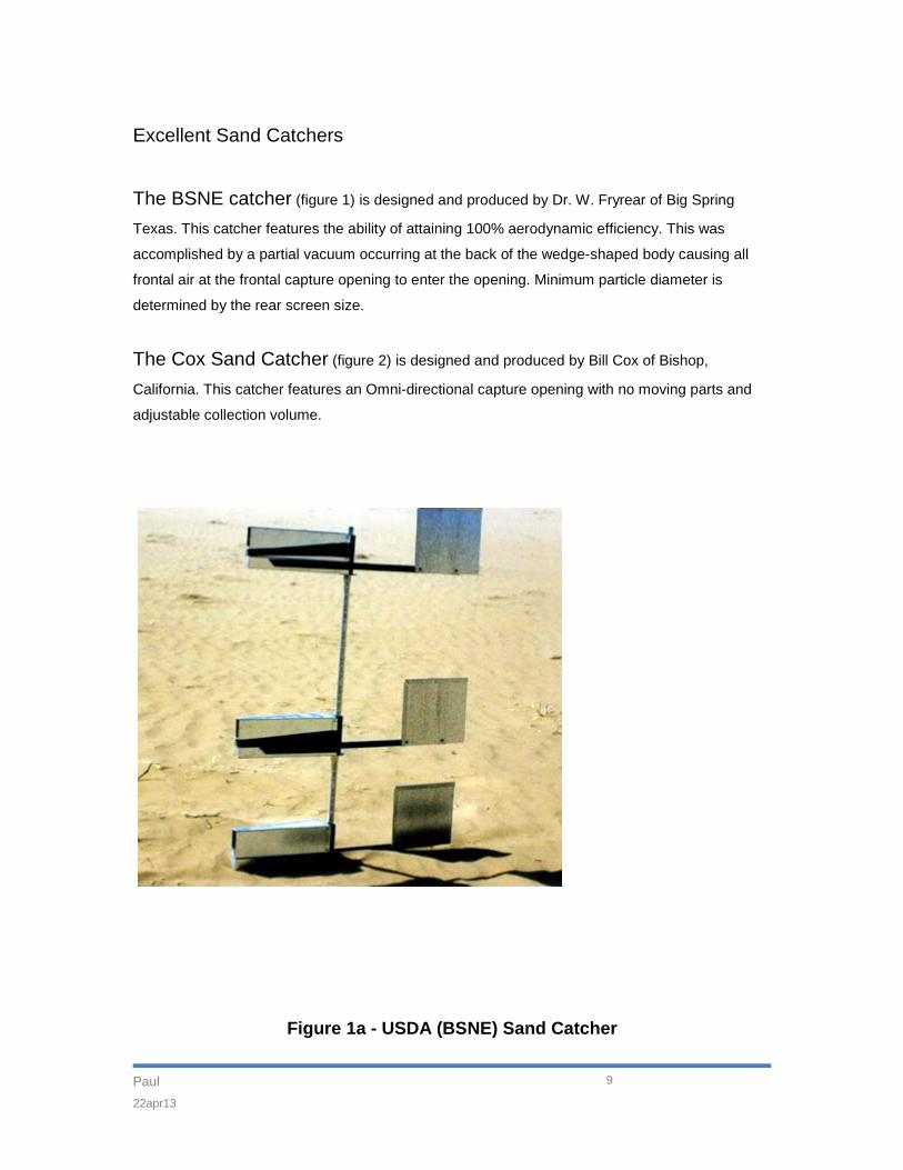
Excellent Sand Catchers

The BSNE catcher (figure 1) is designed and produced by Dr. W. Fryrear of Big Spring

Texas. This catcher features the ability of attaining 100% aerodynamic efficiency. This was

accomplished by a partial vacuum occurring at the back of the wedge-shaped body causing all

frontal air at the frontal capture opening to enter the opening. Minimum particle diameter is

determined by the rear screen size.

The Cox Sand Catcher (figure 2) is designed and produced by Bill Cox of Bishop,

California. This catcher features an Omni-directional capture opening with no moving parts and

adjustable collection volume.

Figure 1a - USDA (BSNE) Sand Catcher

Paul 22apr13

10

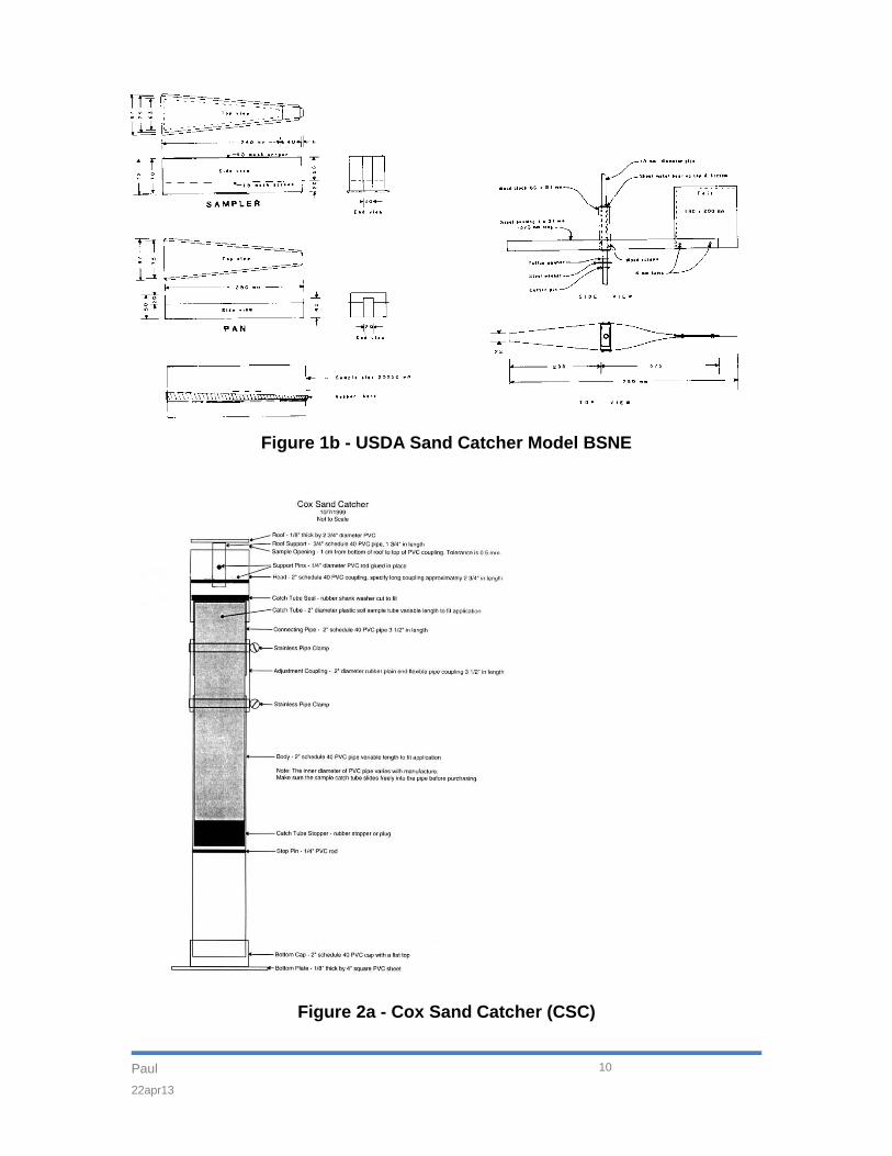
Figure 1b - USDA Sand Catcher Model BSNE

Figure 2a - Cox Sand Catcher (CSC)

Paul 22apr13

11

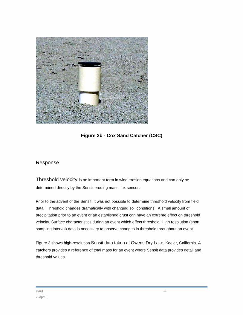
Figure 2b - Cox Sand Catcher (CSC)

Response

Threshold velocity is an important term in wind erosion equations and can only be

determined directly by the Sensit eroding mass flux sensor.

Prior to the advent of the Sensit, it was not possible to determine threshold velocity from field

data. Threshold changes dramatically with changing soil conditions. A small amount of

precipitation prior to an event or an established crust can have an extreme effect on threshold

velocity. Surface characteristics during an event which effect threshold. High resolution (short

sampling interval) data is necessary to observe changes in threshold throughout an event.

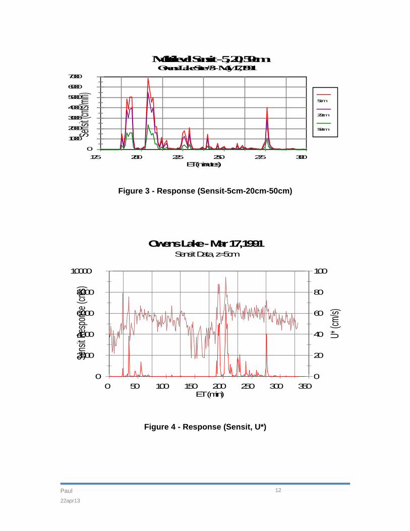
Figure 3 shows high-resolution Sensit data taken at Owens Dry Lake, Keeler, California. A

catchers provides a reference of total mass for an event where Sensit data provides detail and

threshold values.

Paul 22apr13

12

0

1000

2000

3000

4000

5000

6000

7000

Sensit (

cnts/min

)

175 200 225 250 275 300 ET (minutes)

5cm

20cm

50cm

Multilevel Sensit - 5, 20, 50cmOwens Lake Site #3 - May 17,1991

Figure 3 - Response (Sensit-5cm-20cm-50cm)

0

2000

4000

6000

8000

10000

Sens

it Res

pons

e (cn

ts)

0

20

40

60

80

100

U* (c

m/s)

0 50 100 150 200 250 300 350 ET (min)

Owens Lake - Mar 17,1991Sensit Data, z=5cm

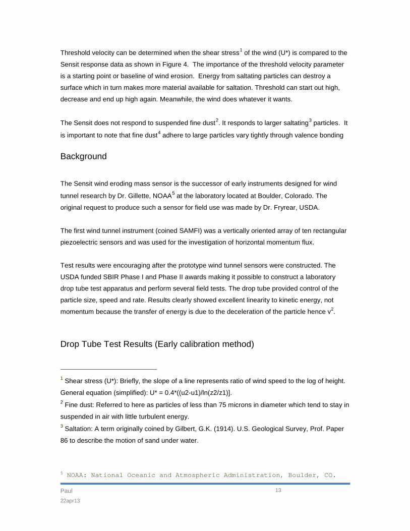
Figure 4 - Response (Sensit, U*)

Paul 22apr13

13

Threshold velocity can be determined when the shear stress1

of the wind (U*) is compared to the

Sensit response data as shown in Figure 4. The importance of the threshold velocity parameter

is a starting point or baseline of wind erosion. Energy from saltating particles can destroy a

surface which in turn makes more material available for saltation. Threshold can start out high,

decrease and end up high again. Meanwhile, the wind does whatever it wants.

The Sensit does not respond to suspended fine dust2. It responds to larger saltating3 particles. It

is important to note that fine dust4

Background

adhere to large particles vary tightly through valence bonding

The Sensit wind eroding mass sensor is the successor of early instruments designed for wind

tunnel research by Dr. Gillette, NOAA5

at the laboratory located at Boulder, Colorado. The

original request to produce such a sensor for field use was made by Dr. Fryrear, USDA.

The first wind tunnel instrument (coined SAMFI) was a vertically oriented array of ten rectangular

piezoelectric sensors and was used for the investigation of horizontal momentum flux.

Test results were encouraging after the prototype wind tunnel sensors were constructed. The

USDA funded SBIR Phase I and Phase II awards making it possible to construct a laboratory

drop tube test apparatus and perform several field tests. The drop tube provided control of the

particle size, speed and rate. Results clearly showed excellent linearity to kinetic energy, not

momentum because the transfer of energy is due to the deceleration of the particle hence v2

.

Drop Tube Test Results (Early calibration method)

1 Shear stress (U*): Briefly, the slope of a line represents ratio of wind speed to the log of height.

General equation (simplified): U* = 0.4*((u2-u1)/ln(z2/z1)]. 2 Fine dust: Referred to here as particles of less than 75 microns in diameter which tend to stay in

suspended in air with little turbulent energy. 3 Saltation: A term originally coined by Gilbert, G.K. (1914). U.S. Geological Survey, Prof. Paper

86 to describe the motion of sand under water.

5 NOAA: National Oceanic and Atmospheric Administration, Boulder, CO.

Paul 22apr13

14

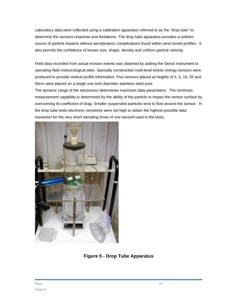
Laboratory data were collected using a calibration apparatus referred to as the "drop tube" to

determine the sensors response and limitations. The drop tube apparatus provides a uniform

source of particle impacts without aerodynamic complications found within wind tunnel profiles. It

also permits the confidence of known size, shape, density and uniform particle velocity.

Field data recorded from actual erosion events was obtained by adding the Sensit instrument to

operating field meteorological sites. Specially constructed multi-level kinetic energy sensors were

produced to provide vertical profile information. Five sensors placed at heights of 2, 5, 10, 20 and

50cm were placed on a single one-inch diameter stainless steel post.

The dynamic range of the electronics determines maximum data parameters. The minimum

measurement capability is determined by the ability of the particle to impact the sensor surface by

overcoming its coefficient of drag. Smaller suspended particles tend to flow around the sensor. In

the drop tube tests electronic sensitivity were set high to obtain the highest possible data

resolution for the very short sampling times of one second used in the tests.

Figure 5 - Drop Tube Apparatus

Paul 22apr13

15

New Model H14-LIN Radial Symmetry Lab Test

The Model H14-LIN replaces all previous models. A new standard output is a 50uS wide pulse

whose height varies with impacting energy. There is one variable height pulse for each particle

impact. This output is referred to as the PHA (pulse height analyzer) output. The PHA output

provides a new per-particle data tool permitting detailed laboratory calibrations.

The height of the pulse can be calibrated to individual particle impact energies providing an

impact energy reference. Useful, but remember field data must always be referenced to a

catcher mass to exclude a multitude of anomalies unique to the site and provide proper units.

The PHA output provides an analog per-impact response value that is an ideal signal to test the

sensor’s minimum / maximum impact energy limits and characterize the radial response pattern

for symmetry.

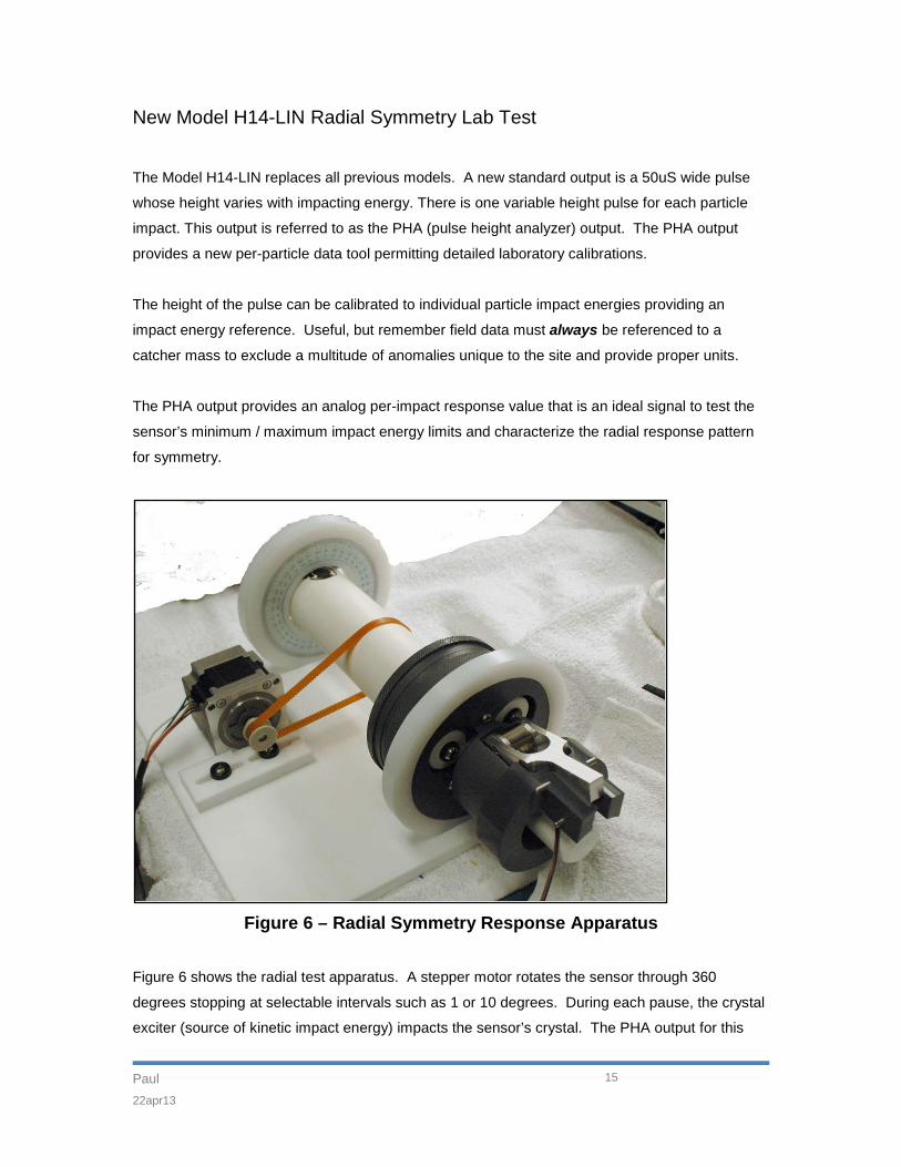
Figure 6 – Radial Symmetry Response Apparatus

Figure 6 shows the radial test apparatus. A stepper motor rotates the sensor through 360

degrees stopping at selectable intervals such as 1 or 10 degrees. During each pause, the crystal

exciter (source of kinetic impact energy) impacts the sensor’s crystal. The PHA output for this

Paul 22apr13

16

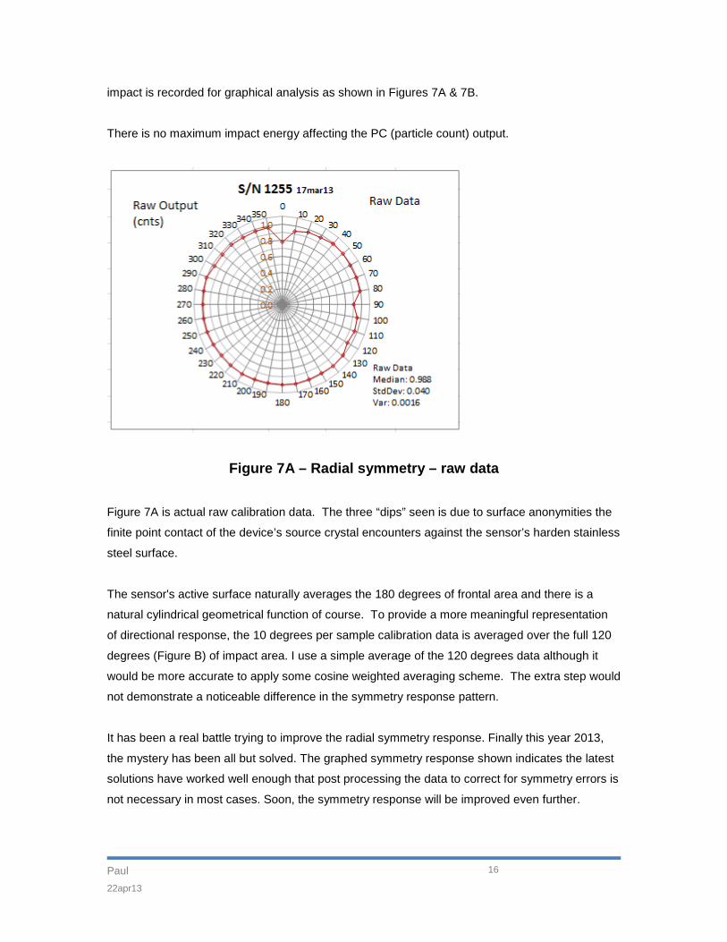
impact is recorded for graphical analysis as shown in Figures 7A & 7B.

There is no maximum impact energy affecting the PC (particle count) output.

Figure 7A – Radial symmetry – raw data

Figure 7A is actual raw calibration data. The three “dips” seen is due to surface anonymities the

finite point contact of the device’s source crystal encounters against the sensor’s harden stainless

steel surface.

The sensor's active surface naturally averages the 180 degrees of frontal area and there is a

natural cylindrical geometrical function of course. To provide a more meaningful representation

of directional response, the 10 degrees per sample calibration data is averaged over the full 120

degrees (Figure B) of impact area. I use a simple average of the 120 degrees data although it

would be more accurate to apply some cosine weighted averaging scheme. The extra step would

not demonstrate a noticeable difference in the symmetry response pattern.

It has been a real battle trying to improve the radial symmetry response. Finally this year 2013,

the mystery has been all but solved. The graphed symmetry response shown indicates the latest

solutions have worked well enough that post processing the data to correct for symmetry errors is

not necessary in most cases. Soon, the symmetry response will be improved even further.

Paul 22apr13

17

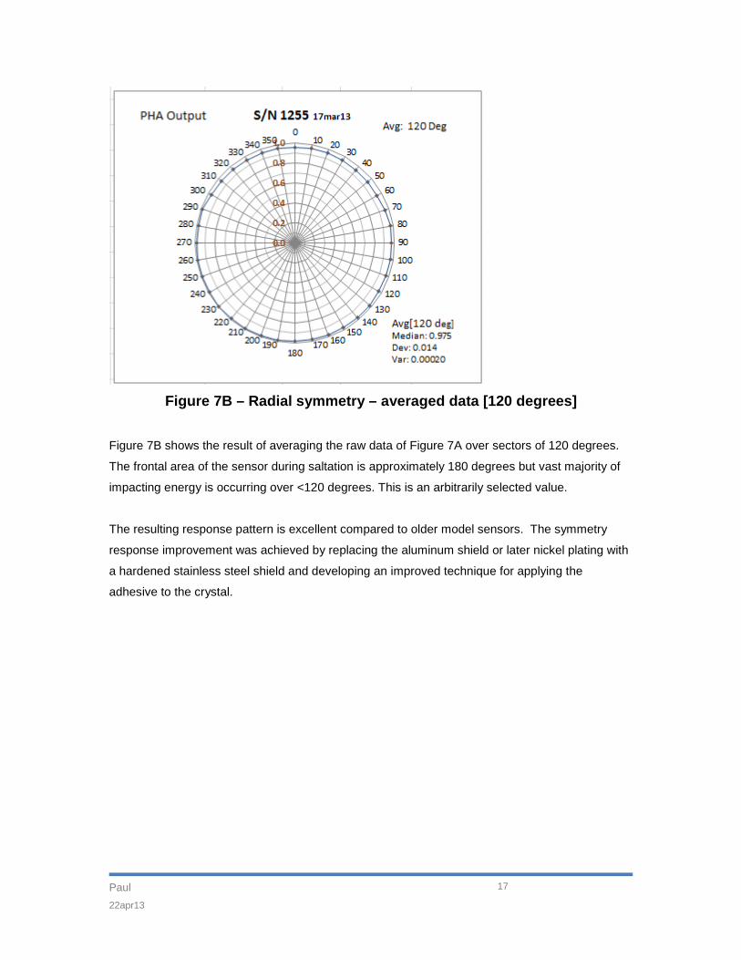
Figure 7B – Radial symmetry – averaged data [120 degrees]

Figure 7B shows the result of averaging the raw data of Figure 7A over sectors of 120 degrees.

The frontal area of the sensor during saltation is approximately 180 degrees but vast majority of

impacting energy is occurring over <120 degrees. This is an arbitrarily selected value.

The resulting response pattern is excellent compared to older model sensors. The symmetry

response improvement was achieved by replacing the aluminum shield or later nickel plating with

a hardened stainless steel shield and developing an improved technique for applying the

adhesive to the crystal.

Paul 22apr13

18

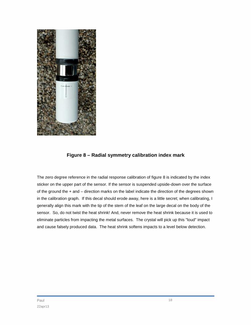
Figure 8 – Radial symmetry calibration index mark

The zero degree reference in the radial response calibration of figure 8 is indicated by the index

sticker on the upper part of the sensor. If the sensor is suspended upside-down over the surface

of the ground the + and – direction marks on the label indicate the direction of the degrees shown

in the calibration graph. If this decal should erode away, here is a little secret; when calibrating, I

generally align this mark with the tip of the stem of the leaf on the large decal on the body of the

sensor. So, do not twist the heat shrink! And, never remove the heat shrink because it is used to

eliminate particles from impacting the metal surfaces. The crystal will pick up this "loud" impact

and cause falsely produced data. The heat shrink softens impacts to a level below detection.

Paul 22apr13

19

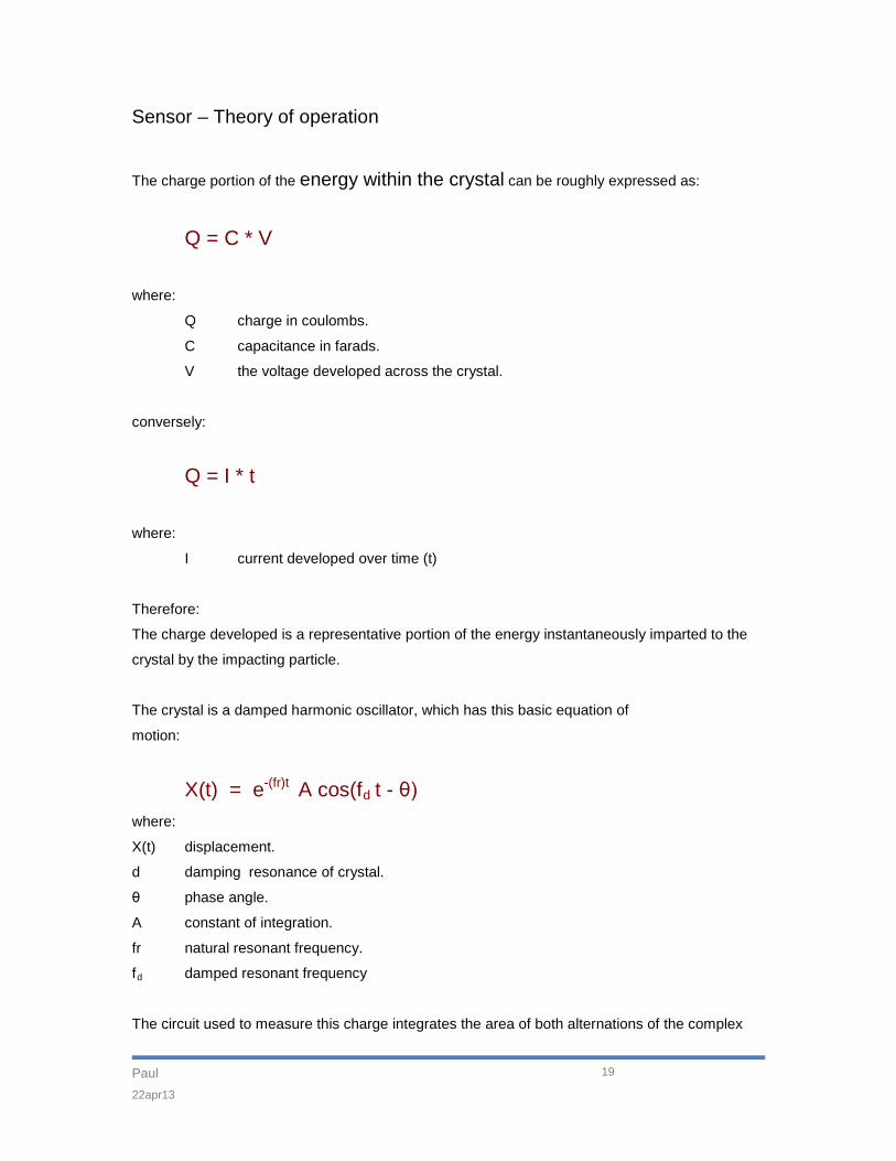
Sensor – Theory of operation

The charge portion of the energy within the crystal can be roughly expressed as:

Q = C * V

where:

Q charge in coulombs.

C capacitance in farads.

V the voltage developed across the crystal.

conversely:

Q = I * t

where:

I current developed over time (t)

Therefore:

The charge developed is a representative portion of the energy instantaneously imparted to the

crystal by the impacting particle.

The crystal is a damped harmonic oscillator, which has this basic equation of

motion:

X(t) = e-(fr)t A cos(fd

where:

t - θ)

X(t) displacement.

d damping resonance of crystal.

θ phase angle.

A constant of integration.

fr natural resonant frequency.

fd

damped resonant frequency

The circuit used to measure this charge integrates the area of both alternations of the complex

Paul 22apr13

20

damped waveform from every impact. When the output of the integrator reaches a

predetermined voltage, the integrator is reset. This reset is stretched to become the output pulse

or data produced by the instrument.

Each output pulse of the instrument represents:

⌠t

KE = │ m V

p

⌡

2 dt

where:

KE One kinetic energy instrument data unit.

Vp

m Mass of each particle.

Particle velocity.

t Time to accumulate one data unit.

Instrument Calibration Constants (Lab & Field)

There are two calibration constants common to the sensor, the laboratory drop tube and the field

calibration constant. Both are used to convert the sensor response to kinetic energy. The field

calibration (method #2) constant has the capability of allowing particle velocity estimation for

every data point.

The old method lab cal (drop tube) involves known measurements of mass, velocity and kinetic

energy. The new radial response calibrator Figure 6 is expected to soon replace the drop tube

apparatus for static impacting energy calibrations.

The field cal makes use of known mass, kinetic energy and a particle velocity term proportional

to the driving force of the wind (U*).

Paul 22apr13

21

Laboratory Drop Tube Cal

The laboratory cal (KL

) is accomplished using the drop tube apparatus previously described.

The lab cal converts the sensor response (KE) to units of kinetic energy using a known mass (m)

and known particle velocity (Vp) satisfying the kinetic energy equation.

KL = m / 2 ∑ [ KE / Vp2

where:

]

m catcher mass

KE Sensit raw response per sampling period

Vp particle velocity

Field Cal (Simplified)

The simplified field cal (KF) relates the total sensor response to total mass allowing the Sensit

to provide a representation of estimated mass flux. Most Sensit users prefer this simple

relationship because empirical tests conducted by the United States Department of Agriculture

(figure 9a), Great Basin Air Pollution Control District (figure 9b) and others consistently

demonstrate an linear relationship between Sensit response to catcher mass. The field cal (Kr

)

assumes the Sensit response is proportional to saltating mass flux for active area and height of

the sensor.

Paul 22apr13

22

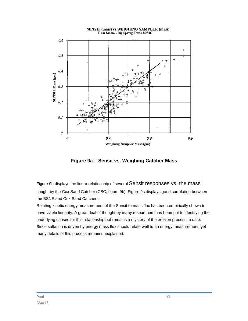
Figure 9a – Sensit vs. Weighing Catcher Mass

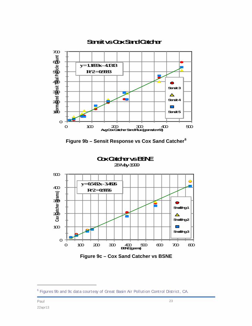
Figure 9b displays the linear relationship of several Sensit responses vs. the mass caught by the Cox Sand Catcher (CSC, figure 9b). Figure 9c displays good correlation between

the BSNE and Cox Sand Catchers.

Relating kinetic energy measurement of the Sensit to mass flux has been empirically shown to

have viable linearity. A great deal of thought by many researchers has been put to identifying the

underlying causes for this relationship but remains a mystery of the erosion process to date.

Since saltation is driven by energy mass flux should relate well to an energy measurement, yet

many details of this process remain unexplained.

Paul 22apr13

23

0

100

200

300

400

500

600

700 No

rmaliz

ed Se

nsit T

otal P

article

Coun

t

0 100 200 300 400 500 Avg Cox Catcher Sand Flux (grams/cm̂2)

Sensit 3

Sensit 4

Sensit 5

Sensit vs Cox Sand Catcher

y = 1.1833x - 4.1313R̂2 = 0.9933

0

100

200

300

400

500

Cax C

atche

r (gram

s)

0 100 200 300 400 500 600 700 800 BSNE (grams)

Small/ng-1

Small/ng-2

Small/ng-3

Cox Catcher vs BSNE28-May-1999

y = 0.5432x - 3.4826R̂2 = 0.9956

Figure 9b – Sensit Response vs Cox Sand Catcher6

Figure 9c – Cox Sand Catcher vs BSNE

6 Figures 9b and 9c data courtesy of Great Basin Air Pollution Control District, CA.

Paul 22apr13

24

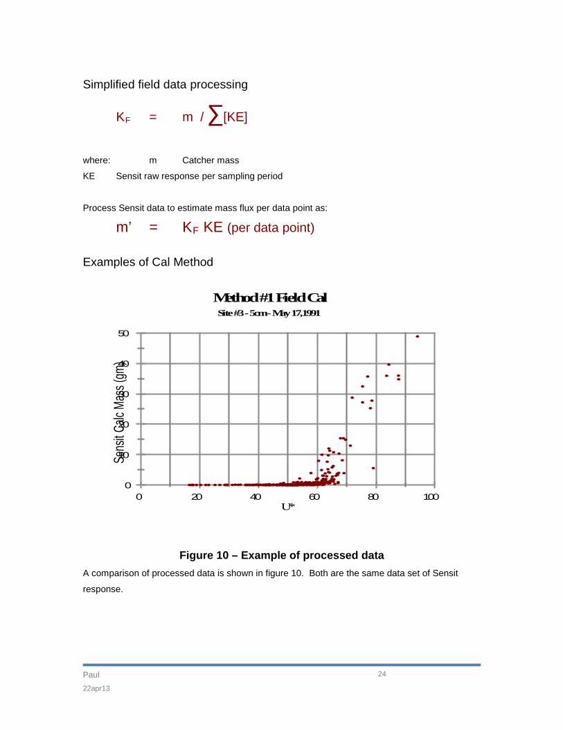
Simplified field data processing

KF

= m / ∑[KE]

where: m Catcher mass

KE Sensit raw response per sampling period

Process Sensit data to estimate mass flux per data point as:

m’ = KF

Examples of Cal Method

KE (per data point)

Figure 10 - Method

Figure 10 – Example of processed data A comparison of processed data is shown in figure 10. Both are the same data set of Sensit

response.

0

10

20

30

40

50

Sens

it Calc

Mas

s (gm

)

0 20 40 60 80 100 U*

Method #1 Field CalSite #3 - 5cm - May 17,1991

Paul 22apr13

25

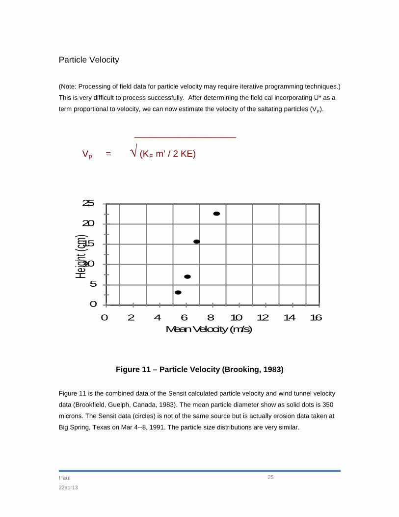
Particle Velocity

(Note: Processing of field data for particle velocity may require iterative programming techniques.)

This is very difficult to process successfully. After determining the field cal incorporating U* as a

term proportional to velocity, we can now estimate the velocity of the saltating particles (Vp

).

____________________

Vp = √ (KF

m’ / 2 KE)

0

5

10

15

20

25

Heigh

t (cm)

0 2 4 6 8 10 12 14 16 Mean Velocity (m/s)

Figure 11 – Particle Velocity (Brooking, 1983)

Figure 11 is the combined data of the Sensit calculated particle velocity and wind tunnel velocity

data (Brookfield, Guelph, Canada, 1983). The mean particle diameter show as solid dots is 350

microns. The Sensit data (circles) is not of the same source but is actually erosion data taken at

Big Spring, Texas on Mar 4--8, 1991. The particle size distributions are very similar.

Paul 22apr13

26

0

200

400

600

800

1000 Pa

rticle

Vel (c

m/s)

0 20 40 60 80 100 U* (cm/s)

Particle Velocity

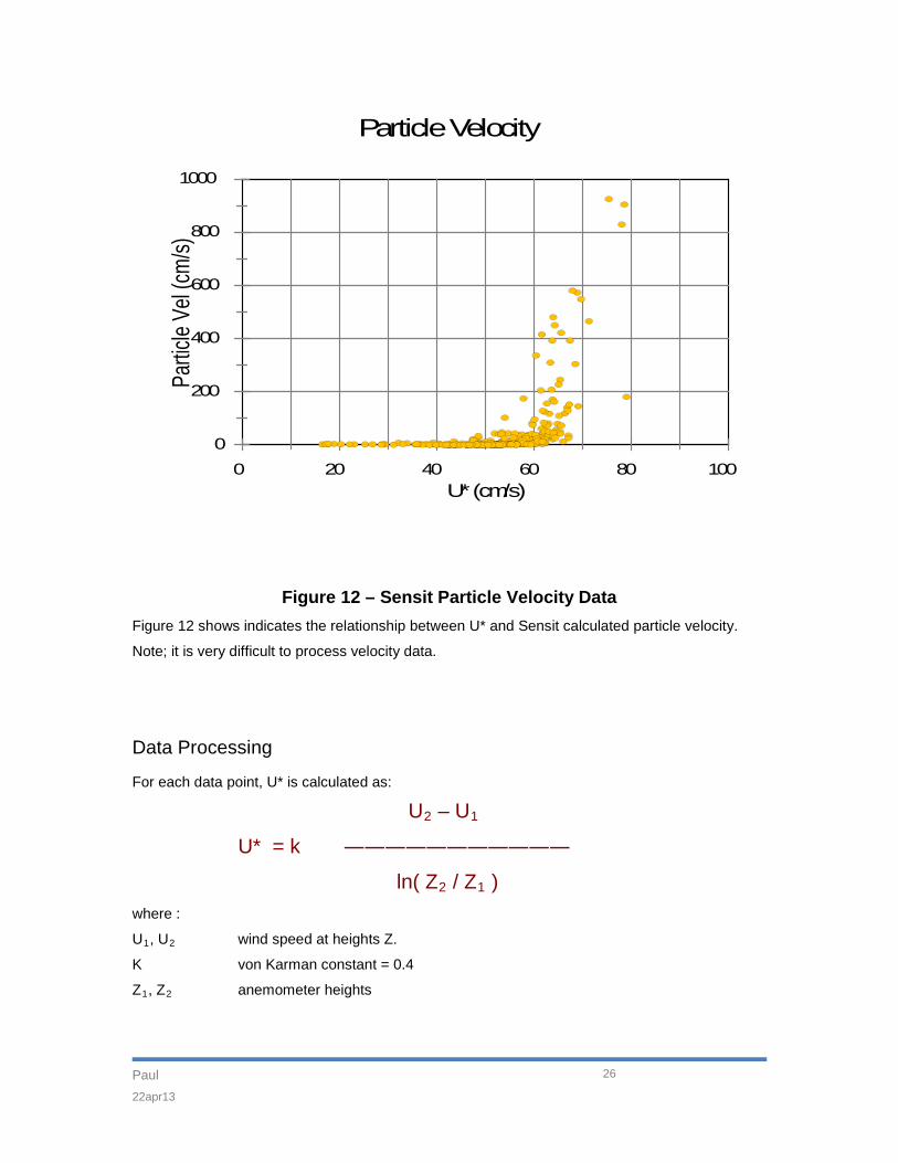
Figure 12 – Sensit Particle Velocity Data Figure 12 shows indicates the relationship between U* and Sensit calculated particle velocity.

Note; it is very difficult to process velocity data.

Data Processing

For each data point, U* is calculated as:

U2 – U1

U* = k ―――――――――――

ln( Z2 / Z1

where :

)

U1, U2

K von Karman constant = 0.4

wind speed at heights Z.

Z1, Z2

anemometer heights

Paul 22apr13

27

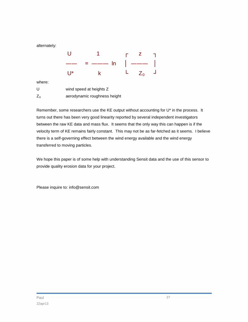
alternately:

U 1 ┌ z ┐

―― = ――― ln │ ――― │

U* k └ Z0

where:

┘

U wind speed at heights Z

Z0

aerodynamic roughness height

Remember, some researchers use the KE output without accounting for U* in the process. It

turns out there has been very good linearity reported by several independent investigators

between the raw KE data and mass flux. It seems that the only way this can happen is if the

velocity term of KE remains fairly constant. This may not be as far-fetched as it seems. I believe

there is a self-governing effect between the wind energy available and the wind energy

transferred to moving particles.

We hope this paper is of some help with understanding Sensit data and the use of this sensor to

provide quality erosion data for your project.

Please inquire to: info@sensit.com

Paul 22apr13

28

Figure 13A & B – Electrical Hookup Wiring Code

Model H11B wiring color code.

Model H14-LIN wiring color code.

POS

N EG

D ATALOGGER

P1 P2V+Gnd

SE

NS

IT

Black

W hite

Brow n

R ed

(KE)

(KEpw )

(Gnd)

(+12V)

Model 11B2

FIELD WIRING DIAGRAM

SENSIT

(PC)

B lue (PCpw)

KW pw PCpw

A lternate outputs*

*K E & P C toggeled to form pulse width m odulation

B RN & WHITE outputs: CM OS /TTL (+Q)

Power: 12VDC @90ma

Nov. 2, 2006

Green

(New W ire Color Code)

Paul 22apr13

29

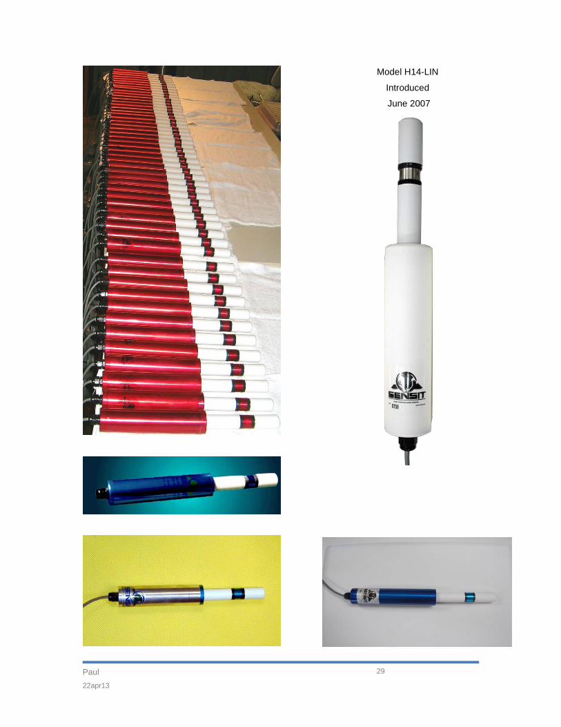
Model H14-LIN

Introduced

June 2007