Embed Size (px)
Citation preview

NASA Technical Memorandum 4804
A Summary of Numerous Strain-Gage Load Calibrations on Aircraft Wings and Tails in a Technology Format
Jerald M. Jenkins and V. Michael DeAngelis
July 1997

National Aeronautics and Space Administration
Office of Management
Scientific and Technical Information Program
1997
NASA Technical Memorandum 4804
A Summary of Numerous Strain-Gage Load Calibrations on Aircraft Wings and Tails in a Technology Format
Jerald M. Jenkins and V. Michael DeAngelis
Dryden Flight Research CenterEdwards, California

ABSTRACT
Fifteen aircraft structures that were calibrated for flight loads using strain gages are examined. The primarypurpose of this paper is to document important examples of load calibrations on airplanes during the past fourdecades. The emphasis is placed on studying the physical procedures of calibrating strain-gaged structures and allthe supporting analyses and computational techniques that have been used. The results and experiences obtainedfrom actual data from 14 structures (on 13 airplanes and 1 laboratory test structure) are presented. This group ofstructures includes fins, tails, and wings with a wide variety of aspect ratios. Straight-wing, swept-wing, and delta-wing configurations are studied. Some of the structures have skin-dominant construction; others are spar-dominant. Anisotropic materials, heat shields, corrugated components, nonorthogonal primary structures, andtruss-type structures are particular characteristics that are included.
NOMENCLATURE
A area, in2
aij element in an array of numbers
Aij a notable element in an array of numbers
AL loaded area or lower area, in2
AT total area, in2
AU upper area, in2
B bending moment, in-lbf
c distance to outer fiber from neutral axis, h/2, in.
CR relevance coefficient, nondimensional
E modulus of elasticity, lbf/in2
eo output voltage, V
EX excitation voltage, V
F. S. fuselage station
G shear modulus, lbf/in2
GF gage factor, nondimensional
h distance between upper and lower centroids, in.
HiMAT Highly Maneuverable Aircraft Technology
HWTS Hypersonic Wing Test Structure
i arbitrary integer
I moment of inertia, in4
IBAR moment of inertia of a beam element, in4
IC influence coefficient, output/lbf
j arbitrary integer
J polar moment of inertia of cross-sectional area, in4
K linear constant, nondimensional
L load or left load, lbf

M bending moment, in-lbf
n arbitrary integer
N strain-gage bridge factor, nondimensional
p cell perimeter, in.
P load, lbf
q shear flow, lbf/in
Q defined as Ah/4, in3
R right load, lbf
SG strain gage
t skin thickness, in.
tm thickness of model, in.
tw thickness of wing, in.
TACT Transonic Aircraft Technology
V section shear load, lbf
x Cartesian coordinate
y Cartesian coordinate
yL distance to lower centroid, in.
yU distance to upper centroid, in.
z Cartesian coordinate
β constant, nondimensional
γ shear strain, nondimensional
δ deflection, in., or voltage change resulting from straining the active arms of a strain-gage bridge, V
δcal reference voltage change resulting from shunting a calibrated resistor across one arm of a strain-gage bridge, V
ε normal strain, nondimensional
η span fraction
θ angle of rotation, deg
Λ wing sweep angle, deg
µ nondimensional strain-gage response, δ/δcal
ξ chord fraction
σ normal stress, lbf/in2
τ shear stress, lbf/in2
υ Poisson’s ratio, nondimensional
φ angle of rotation, deg
2
INTRODUCTION
The idea of using calibrated strain gages through influence-coefficient formats to measure flight loads onairplane components likely evolved from similar interests in other scientific fields. The common denominator wasthe response of the structure at some discrete location to load, which is the well-known influence coefficient. Themotivation to define the loads on lifting and stabilizing surfaces was greatly enhanced by rapidly evolving aircraftperformance in the 1930 to 1950 time period. Major efforts to measure loads with strain gages were ongoing in the1940’s; however, the approach was not solidified until 1954. The idea was perpetuated by Skopinske, Aiken, andHuston1 in their 1954 report. The linear regression approach to develop mathematical load equations from strain-gage responses obtained from physically applying loads to an airplane wing or other structural part is still theprimary and only commonly used method today. Other mathematical approaches such as singular-valueddecompositions2 are being investigated and may someday prove advantageous; however, these approaches need tobe demonstrated.
The complexity of load calibrations using strain gages has increased as the complexity of the structure andmaterials has also increased. Straight wings and tails with few and dominant spars characterized early airplanestructures. Swept wings and delta wings with many spars emerged later. Complex structures such as integratedhoneycomb skins and corrugated webs led to strain gages being located in less-than-optimum places. Compositematerials, many of which are anisotropic, also emerged to further complicate the situation. High-speed airplanesexperienced significant aerodynamic heating that affected the nature of strain-gage responses. All of these factorschallenged the load-measurement engineer to adapt and create new and better approaches and tools.
The increased cost associated with conducting load calibrations on aircraft introduced an economic factor thathas impacted recent aircraft programs. Aircraft developers are under extreme economic pressure to find less-expensive alternatives to the expensive strain-gage load calibrations. Advanced computer capabilities haveprovided new and better ways to visualize the mathematical situations, enhancing the load measurer’s ability tooptimize engineering judgements. All of these factors, circumstances, and tools in aggregate constitute the scienceof measuring loads with calibrated strain gages on aircraft.
The purpose of this paper is to document important examples of load calibrations on aircraft, many of whichwere flight-tested at the NASA Dryden Flight Research Facility at Edwards, California, during the past 30 years.The technical experiences and approaches leading to optimum load calibrations will be presented. The latest toolswill be identified, and examples and future directions for load calibrations will be projected.
The primary emphasis of this paper will be on studying the total physical procedures of calibrating strain-gaged structures and all the supporting analyses and computational techniques that have been used. Theload-calibration science will be studied using the results and experiences obtained from the actual data and fromefforts involving 14 structures on 13 aircraft and 1 laboratory test structure. The structures included in the effortare as follows:
• the M2-F2 tip fin
• the X-24 tip fin
• the HL-10 center fin
• the X-24 center fin
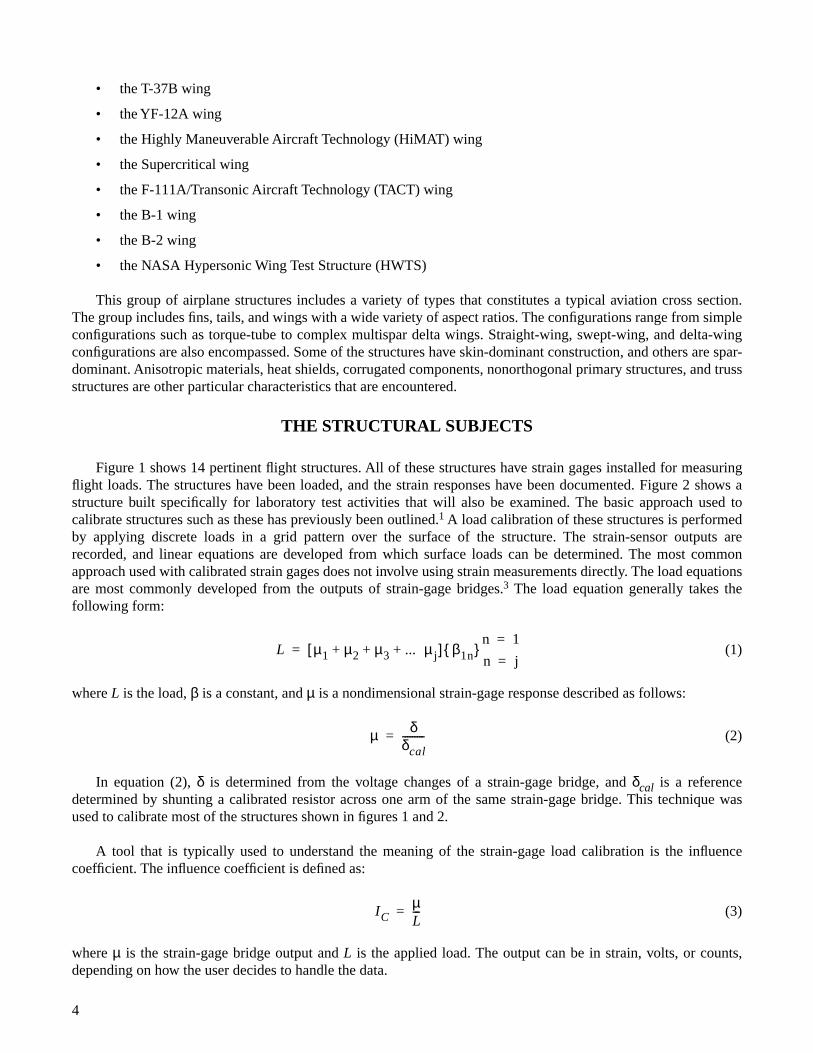
• the X-15 horizontal tail
• the F-89 wing
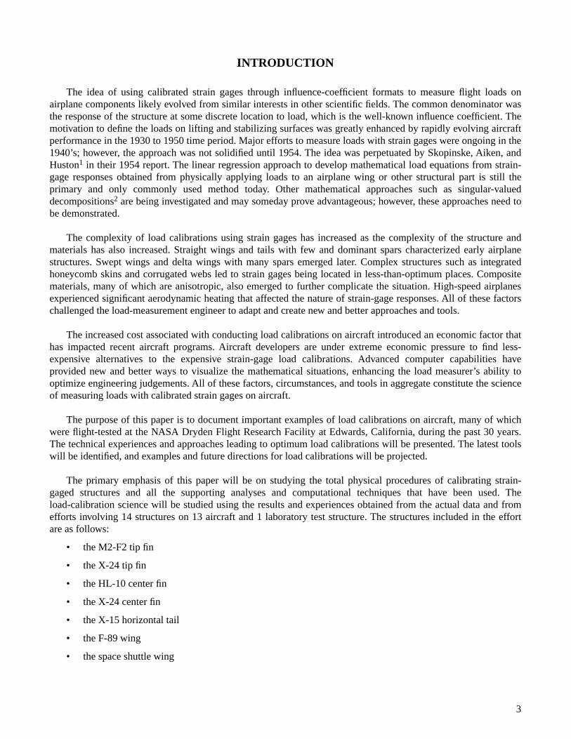
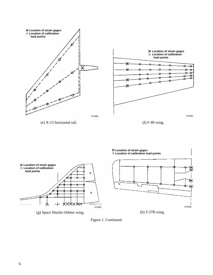
• the space shuttle wing
3
• the T-37B wing
• the YF-12A wing
• the Highly Maneuverable Aircraft Technology (HiMAT) wing
• the Supercritical wing
• the F-111A/Transonic Aircraft Technology (TACT) wing
• the B-1 wing
• the B-2 wing
• the NASA Hypersonic Wing Test Structure (HWTS)
This group of airplane structures includes a variety of types that constitutes a typical aviation cross section.The group includes fins, tails, and wings with a wide variety of aspect ratios. The configurations range from simpleconfigurations such as torque-tube to complex multispar delta wings. Straight-wing, swept-wing, and delta-wingconfigurations are also encompassed. Some of the structures have skin-dominant construction, and others are spar-dominant. Anisotropic materials, heat shields, corrugated components, nonorthogonal primary structures, and trussstructures are other particular characteristics that are encountered.
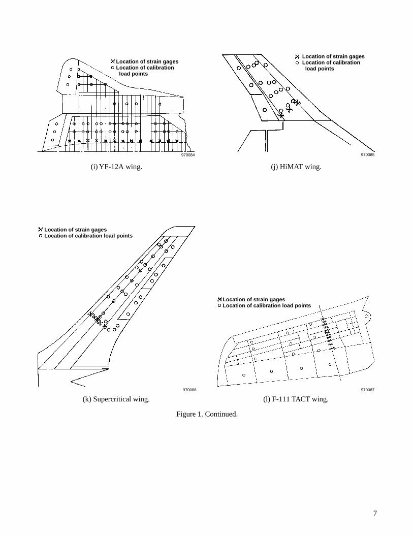
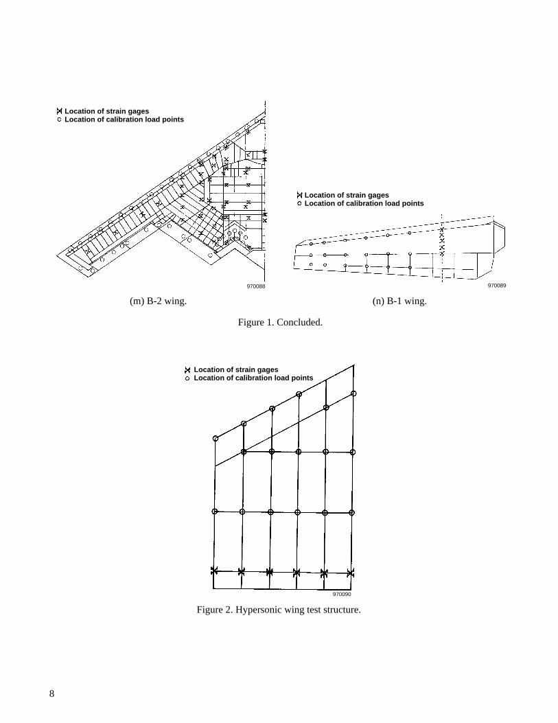
THE STRUCTURAL SUBJECTS
Figure 1 shows 14 pertinent flight structures. All of these structures have strain gages installed for measuringflight loads. The structures have been loaded, and the strain responses have been documented. Figure 2 shows astructure built specifically for laboratory test activities that will also be examined. The basic approach used tocalibrate structures such as these has previously been outlined.1 A load calibration of these structures is performedby applying discrete loads in a grid pattern over the surface of the structure. The strain-sensor outputs arerecorded, and linear equations are developed from which surface loads can be determined. The most commonapproach used with calibrated strain gages does not involve using strain measurements directly. The load equationsare most commonly developed from the outputs of strain-gage bridges.3 The load equation generally takes thefollowing form:
(1)
where L is the load, β is a constant, and µ is a nondimensional strain-gage response described as follows:
(2)
In equation (2), δ is determined from the voltage changes of a strain-gage bridge, and δcal is a referencedetermined by shunting a calibrated resistor across one arm of the same strain-gage bridge. This technique wasused to calibrate most of the structures shown in figures 1 and 2.
A tool that is typically used to understand the meaning of the strain-gage load calibration is the influencecoefficient. The influence coefficient is defined as:
(3)
where µ is the strain-gage bridge output and L is the applied load. The output can be in strain, volts, or counts,depending on how the user decides to handle the data.
L µ1 µ2 µ3 ... µ j+ + +[ ] β 1n{ }n 1=
n j==
µ δδcal---------=
ICµL---=
4

5
Location of strain gagesLocation of calibration load points
970076
(a) M2-F2 tip fin.
Location of strain gagesLocation of calibration load points
970077
(b) X-24A tip fin.
(c) HL-10 center fin. (d) X-24A center fin.
Location of strain gagesLocation of calibration load points
970078
Location of strain gagesLocation of calibration load points
970079
Figure 1. Lifting or stabilizing surfaces studied for load calibration characteristics.
6
Location of strain gagesLocation of calibration load points
970080
970081
Location of strain gagesLocation of calibration load points
970082
Location of strain gagesLocation of calibration load points
970083
Location of strain gagesLocation of calibration load points
(e) X-15 horizontal tail. (f) F-89 wing.
(g) Space Shuttle Orbiter wing. (h) T-37B wing.
Figure 1. Continued.
7
970084
Location of strain gagesLocation of calibration load points
970085
Location of strain gagesLocation of calibration load points
970086
Location of strain gagesLocation of calibration load points
970087
Location of strain gagesLocation of calibration load points
(i) YF-12A wing. (j) HiMAT wing.
(k) Supercritical wing. (l) F-111 TACT wing.
Figure 1. Continued.
8
970088
Location of strain gagesLocation of calibration load points
970089
Location of strain gagesLocation of calibration load points
Figure 1. Concluded.
(m) B-2 wing. (n) B-1 wing.
970090
Location of strain gagesLocation of calibration load points
Figure 2. Hypersonic wing test structure.
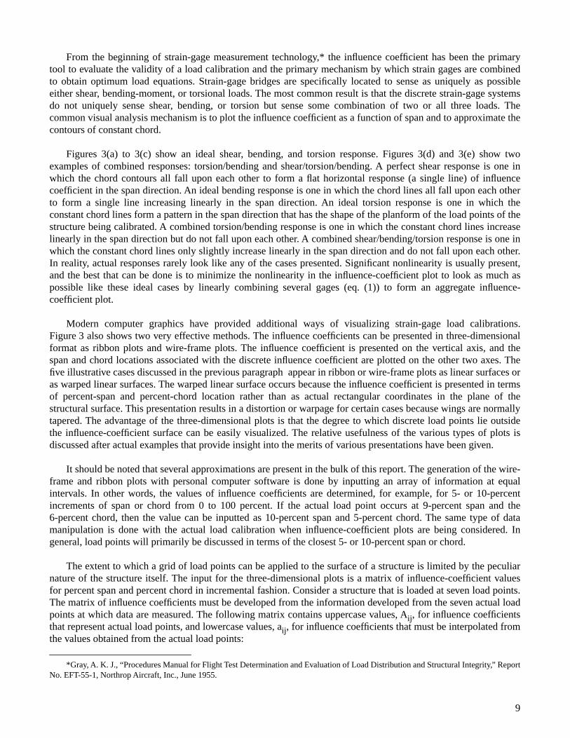
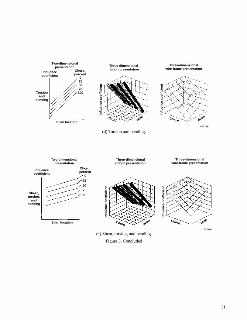
From the beginning of strain-gage measurement technology,* the influence coefficient has been the primarytool to evaluate the validity of a load calibration and the primary mechanism by which strain gages are combinedto obtain optimum load equations. Strain-gage bridges are specifically located to sense as uniquely as possibleeither shear, bending-moment, or torsional loads. The most common result is that the discrete strain-gage systemsdo not uniquely sense shear, bending, or torsion but sense some combination of two or all three loads. Thecommon visual analysis mechanism is to plot the influence coefficient as a function of span and to approximate thecontours of constant chord.
Figures 3(a) to 3(c) show an ideal shear, bending, and torsion response. Figures 3(d) and 3(e) show twoexamples of combined responses: torsion/bending and shear/torsion/bending. A perfect shear response is one inwhich the chord contours all fall upon each other to form a flat horizontal response (a single line) of influencecoefficient in the span direction. An ideal bending response is one in which the chord lines all fall upon each otherto form a single line increasing linearly in the span direction. An ideal torsion response is one in which theconstant chord lines form a pattern in the span direction that has the shape of the planform of the load points of thestructure being calibrated. A combined torsion/bending response is one in which the constant chord lines increaselinearly in the span direction but do not fall upon each other. A combined shear/bending/torsion response is one inwhich the constant chord lines only slightly increase linearly in the span direction and do not fall upon each other.In reality, actual responses rarely look like any of the cases presented. Significant nonlinearity is usually present,and the best that can be done is to minimize the nonlinearity in the influence-coefficient plot to look as much aspossible like these ideal cases by linearly combining several gages (eq. (1)) to form an aggregate influence-coefficient plot.
Modern computer graphics have provided additional ways of visualizing strain-gage load calibrations.Figure 3 also shows two very effective methods. The influence coefficients can be presented in three-dimensionalformat as ribbon plots and wire-frame plots. The influence coefficient is presented on the vertical axis, and thespan and chord locations associated with the discrete influence coefficient are plotted on the other two axes. Thefive illustrative cases discussed in the previous paragraph appear in ribbon or wire-frame plots as linear surfaces oras warped linear surfaces. The warped linear surface occurs because the influence coefficient is presented in termsof percent-span and percent-chord location rather than as actual rectangular coordinates in the plane of thestructural surface. This presentation results in a distortion or warpage for certain cases because wings are normallytapered. The advantage of the three-dimensional plots is that the degree to which discrete load points lie outsidethe influence-coefficient surface can be easily visualized. The relative usefulness of the various types of plots isdiscussed after actual examples that provide insight into the merits of various presentations have been given.
It should be noted that several approximations are present in the bulk of this report. The generation of the wire-frame and ribbon plots with personal computer software is done by inputting an array of information at equalintervals. In other words, the values of influence coefficients are determined, for example, for 5- or 10-percentincrements of span or chord from 0 to 100 percent. If the actual load point occurs at 9-percent span and the6-percent chord, then the value can be inputted as 10-percent span and 5-percent chord. The same type of datamanipulation is done with the actual load calibration when influence-coefficient plots are being considered. Ingeneral, load points will primarily be discussed in terms of the closest 5- or 10-percent span or chord.
The extent to which a grid of load points can be applied to the surface of a structure is limited by the peculiarnature of the structure itself. The input for the three-dimensional plots is a matrix of influence-coefficient valuesfor percent span and percent chord in incremental fashion. Consider a structure that is loaded at seven load points.The matrix of influence coefficients must be developed from the information developed from the seven actual loadpoints at which data are measured. The following matrix contains uppercase values, Aij, for influence coefficientsthat represent actual load points, and lowercase values, aij, for influence coefficients that must be interpolated fromthe values obtained from the actual load points:
*Gray, A. K. J., “Procedures Manual for Flight Test Determination and Evaluation of Load Distribution and Structural Integrity,” ReportNo. EFT-55-1, Northrop Aircraft, Inc., June 1955.
9

10
Influencecoefficient
Two-dimensionalpresentation
Three-dimensionalribbon presentation
Three-dimensionalwire-frame presentation
Shear
970091Span location
0- to 100-percent chord
ChordChordSpan Span
Infl
uen
ce c
oef
fici
ent
Infl
uen
ce c
oef
fici
ent
Influencecoefficient
Two-dimensionalpresentation
Three-dimensionalribbon presentation
Three-dimensionalwire-frame presentation
Bendingmoment
970735
Span location
0- to 100-percentchord Chord Chord
SpanSpan
Infl
uen
ce c
oef
fici
ent
Infl
uen
ce c
oef
fici
ent
Influence coefficient
Two-dimensional presentation
Three-dimensional ribbon presentation
Three-dimensional wire-frame presentation
Torsion
970099Span location
Chord, percent
0 25 50 75
100
ChordChordSpan
Span
Infl
uen
ce c
oef
fici
ent
Infl
uen
ce c
oef
fici
ent
(a) Shear.
(b) Bending moment.
(c) Torsion.
Figure 3. Methods of presenting the common lifting-surface strain-gage responses in terms of influence-coefficient plots.
11
Influencecoefficient
Two-dimensionalpresentation Three-dimensional
ribbon presentationThree-dimensional
wire-frame presentation
Torsionand
bending
970736
Span location
Chord,percent
0255075100
Chord ChordSpanSpan
Infl
uen
ce c
oef
fici
ent
Infl
uen
ce c
oef
fici
ent
970100
Influencecoefficient
Two-dimensionalpresentation
Three-dimensionalribbon presentation
Three-dimensionalwire-frame presentation
Shear,torsion,
andbending
Span location
Chord,percent
0
25
5075
100
ChordChordSpan
Span
Infl
uen
ce c
oef
fici
ent
Infl
uen
ce c
oef
fici
ent
(d) Torsion and bending.
(e) Shear, torsion, and bending.
Figure 3. Concluded
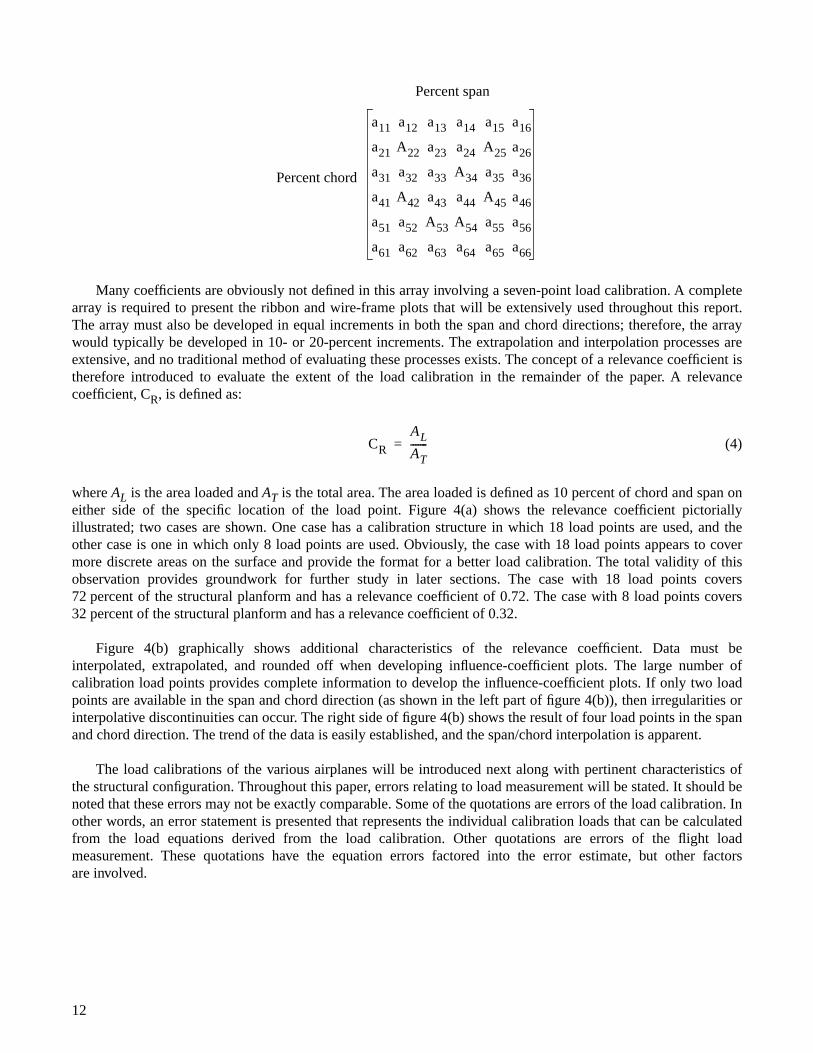
Many coefficients are obviously not defined in this array involving a seven-point load calibration. A completearray is required to present the ribbon and wire-frame plots that will be extensively used throughout this report.The array must also be developed in equal increments in both the span and chord directions; therefore, the arraywould typically be developed in 10- or 20-percent increments. The extrapolation and interpolation processes areextensive, and no traditional method of evaluating these processes exists. The concept of a relevance coefficient istherefore introduced to evaluate the extent of the load calibration in the remainder of the paper. A relevancecoefficient, CR, is defined as:
(4)
where AL is the area loaded and AT is the total area. The area loaded is defined as 10 percent of chord and span oneither side of the specific location of the load point. Figure 4(a) shows the relevance coefficient pictoriallyillustrated; two cases are shown. One case has a calibration structure in which 18 load points are used, and theother case is one in which only 8 load points are used. Obviously, the case with 18 load points appears to covermore discrete areas on the surface and provide the format for a better load calibration. The total validity of thisobservation provides groundwork for further study in later sections. The case with 18 load points covers72 percent of the structural planform and has a relevance coefficient of 0.72. The case with 8 load points covers32 percent of the structural planform and has a relevance coefficient of 0.32.
Figure 4(b) graphically shows additional characteristics of the relevance coefficient. Data must beinterpolated, extrapolated, and rounded off when developing influence-coefficient plots. The large number ofcalibration load points provides complete information to develop the influence-coefficient plots. If only two loadpoints are available in the span and chord direction (as shown in the left part of figure 4(b)), then irregularities orinterpolative discontinuities can occur. The right side of figure 4(b) shows the result of four load points in the spanand chord direction. The trend of the data is easily established, and the span/chord interpolation is apparent.
The load calibrations of the various airplanes will be introduced next along with pertinent characteristics ofthe structural configuration. Throughout this paper, errors relating to load measurement will be stated. It should benoted that these errors may not be exactly comparable. Some of the quotations are errors of the load calibration. Inother words, an error statement is presented that represents the individual calibration loads that can be calculatedfrom the load equations derived from the load calibration. Other quotations are errors of the flight loadmeasurement. These quotations have the equation errors factored into the error estimate, but other factorsare involved.
Percent chord
Percent span
a11 a12 a13 a14 a15 a16
a21 A22 a23 a24 A25 a26
a31 a32 a33 A34 a35 a36
a41 A42 a43 a44 A45 a46
a51 a52 A53 A54 a55 a56
a61 a62 a63 a64 a65 a66
CR
AL
AT-------=
12
13
970092Span, percent
Effective loading area
100806040200
0
20
40
60
80
100
Span, percent100806040200
CR = 0.72
Heavily loaded(18 load points)
Chord,percent
CR = 0.32
Sparsely loaded(8 load points)
970093
Chord
Span
Chord
Final interpolated input for generation of influence-coefficient surface plots
Load-point locations
Low CR calibrationSpan
Chord
Span
Chord
Interpolative incompatibility
Span
Infl
uen
ce c
oef
fici
ent
Infl
uen
ce c
oef
fici
ent
Infl
uen
ce c
oef
fici
ent
Infl
uen
ce c
oef
fici
ent
High CR calibration
(b) Effect of the relevance coefficient on the generation of influence-coefficient input data for ribbon andwire-frame plots.
Figure 4. The relevance coefficient and how input data are generated for the ribbon and wire-frame plots.
(a) Pictorial illustration of the relevance coefficient.
CALIBRATION OF THE AIRCRAFT STRUCTURES
The basic purpose of this section is to present the physical load calibration of the strain gages and thecharacteristics of the response. The number of load points, the location of the load points, the location of the straingages, the structural arrangement, the influence coefficients, and all other circumstances and facts pertinent to theload calibration are presented in this section.
M2-F2 Tip Fin
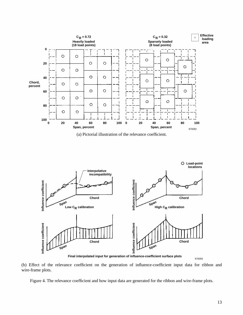
Appendix A shows a three-view sketch of the M2-F2 lifting body. Loads were measured on the tip fin, whichfigure 1(a) shows in more detail. The stabilizing surface is a low-aspect-ratio structure with multiple spars.Figure 1(a) also shows the location of strain gages and an extensive grid of calibration load points. The basicstrain-gage load calibration has been documented,* and the flight results have previously been presented.4 Thirty-five load points were used to calibrate 20 strain-gage bridges located in and around the 7 spars. The very lowaspect ratio of this structure coupled with multiple short spars provided at least one unique strain-gage responsecharacteristic. The three-dimensional ribbon plot (fig. 5) is the primary method used to present data forthis structure.
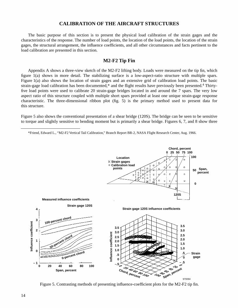
Figure 5 also shows the conventional presentation of a shear bridge (120S). The bridge can be seen to be sensitiveto torque and slightly sensitive to bending moment but is primarily a shear bridge. Figures 6, 7, and 8 show three
*Friend, Edward L., “M2-F2 Vertical Tail Calibration,” Branch Report BR-2, NASA Flight Research Center, Aug. 1966.
14
Figure 5. Contrasting methods of presenting influence-coefficient plots for the M2-F2 tip fin.
Strain gage 120S influence coefficients
120S
Chord, percent
Span,percent
Strain gage 120S
100-percent chord
0-percent chord
50-percent chord
Measured influence coefficients
3.5
Strain gage
3.0
2.52.01.5
1.0
.50
– .5
970094
Chord, percent Span, percent
1001008080
60604040
202000
Infl
uen
ce c
oef
fici
ent
3.5
0 40Span, percent
6020 80
0 25 50 75 100100
50
0
100
Infl
uen
ce c
oef
fici
ent
4
3
– 1
2
1
0
3.0
2.52.01.5
1.0
.50
–.5
LocationStrain gagesCalibration load points
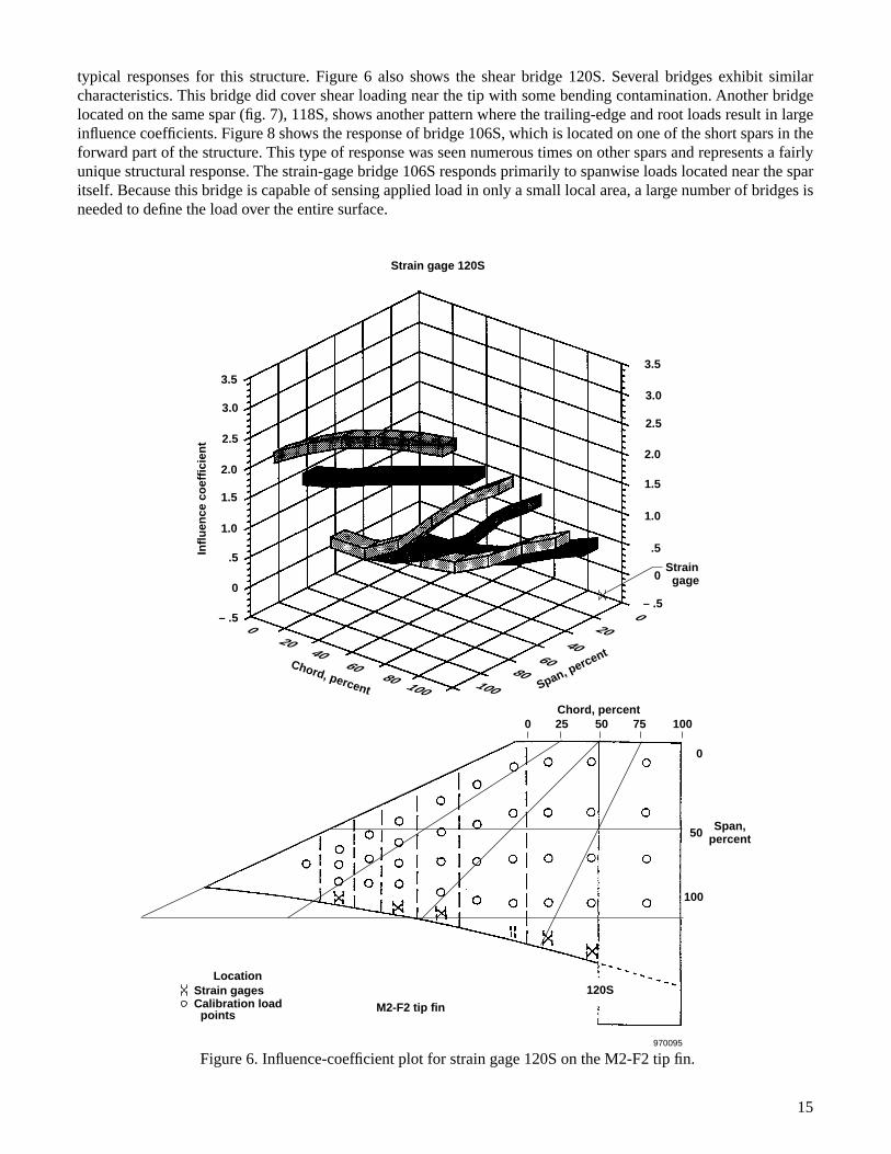
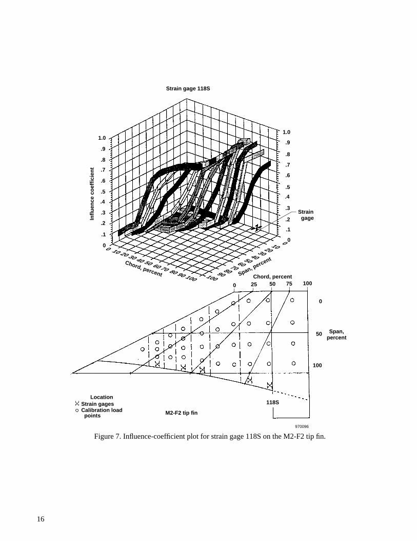
typical responses for this structure. Figure 6 also shows the shear bridge 120S. Several bridges exhibit similarcharacteristics. This bridge did cover shear loading near the tip with some bending contamination. Another bridgelocated on the same spar (fig. 7), 118S, shows another pattern where the trailing-edge and root loads result in largeinfluence coefficients. Figure 8 shows the response of bridge 106S, which is located on one of the short spars in theforward part of the structure. This type of response was seen numerous times on other spars and represents a fairlyunique structural response. The strain-gage bridge 106S responds primarily to spanwise loads located near the sparitself. Because this bridge is capable of sensing applied load in only a small local area, a large number of bridges isneeded to define the load over the entire surface.
15
Strain gage 120S
120S
Chord, percent
Span,percent
M2-F2 tip fin
3.5
Strain gage
3.0
2.5
2.0
1.5
1.0
.5
0
– .5
970095
Chord, percent Span, percent
1001008080
6060
4040
2020
00
Infl
uen
ce c
oef
fici
ent
3.5
0 25 50 75 100
100
50
0
3.0
2.5
2.0
1.5
1.0
.5
0
– .5
LocationStrain gagesCalibration load points
Figure 6. Influence-coefficient plot for strain gage 120S on the M2-F2 tip fin.
16
Strain gage 118S
118S
Chord, percent
Span,percent
M2-F2 tip fin
Strain gage
970096
0 25 50 75 100
100
50
0
1.0
Chord, percent Span, percent
100100809090
8060
507060 70
4040
102030201030
50
00
Infl
uen
ce c
oef
fici
ent
1.0
.9
.8
.7
.6
.5
.4
.3
.2
.1
0
.9
.8
.7
.6
.5
.4
.3
.2
.1
0
LocationStrain gagesCalibration load points
Figure 7. Influence-coefficient plot for strain gage 118S on the M2-F2 tip fin.
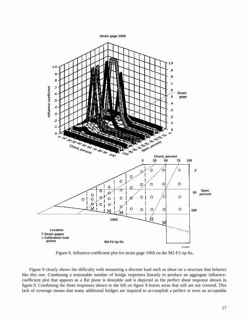
Strain gage 106S
Chord, percent
Span,percent
Strain gage
970097
Chord, percent Span, percent
100100
80909080
6050
7060 70
4040
1020302010
3050
00
0 25 50 75 100
100
50
0
1.0
Infl
uen
ce c
oef
fici
ent
1.0
.9
.8
.7
.6
.5
.4
.3
.2
.1
0
.9
.8
.7
.6
.5
.4
.3
.2
.1
0
LocationStrain gagesCalibration load points
106S
M2-F2 tip fin
Figure 8. Influence-coefficient plot for strain gage 106S on the M2-F2 tip fin.
Figure 9 clearly shows the difficulty with measuring a discrete load such as shear on a structure that behaveslike this one. Combining a reasonable number of bridge responses linearly to produce an aggregate influence-coefficient plot that appears as a flat plane is desirable and is depicted as the perfect shear response shown infigure 9. Combining the three responses shown to the left on figure 9 leaves areas that still are not covered. Thislack of coverage means that many additional bridges are required to accomplish a perfect or even an acceptable
17
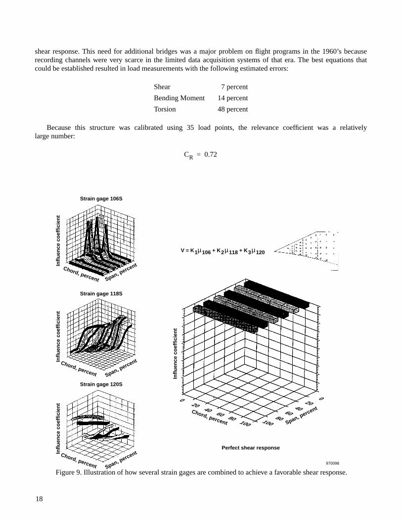
shear response. This need for additional bridges was a major problem on flight programs in the 1960’s becauserecording channels were very scarce in the limited data acquisition systems of that era. The best equations thatcould be established resulted in load measurements with the following estimated errors:
Because this structure was calibrated using 35 load points, the relevance coefficient was a relativelylarge number:
Shear 7 percent
Bending Moment 14 percent
Torsion 48 percent
CR 0.72=
18
970098
Chord, percent
Chord, percent
Span, percent
Span, percent
1001008080
60604040
202000
Infl
uen
ce c
oef
fici
ent
Strain gage 118S
Infl
uen
ce c
oef
fici
ent
Chord, percent Span, percentInfl
uen
ce c
oef
fici
ent
Chord, percent Span, percentInfl
uen
ce c
oef
fici
ent
Strain gage 106S
V = K1µ106 + K2µ118 + K3µ120
Perfect shear response
Strain gage 120S
Figure 9. Illustration of how several strain gages are combined to achieve a favorable shear response.
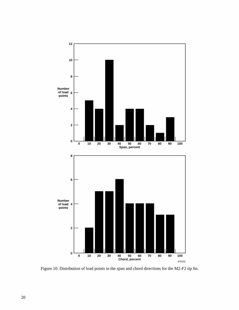
Figure 10 shows the distribution of the calibration load points in terms of span and chord. The large number ofload points provides extensive coverage that leads to the large relevance coefficient of 0.72. The large relevancecoefficient logically would imply a situation where very accurate loads would be measured. This accuracy wascertainly not the case for at least the bending moment and torsion. The most likely reason for the poor accuracy isthe limited number of recording channels available to record flight data. More flight recording channels wouldallow more strain-gage bridges to be used in the equations, which would likely better define the overall response tosurface loads on the structure than when limited channels are available.
X-24A Tip Fin
Appendix A shows a three-view sketch of the X-24 lifting body. Figure 1(b) shows the tip fin in more detailand where calibration load points are located along with strain gages. The stabilizing surface can be seen to be alow-aspect-ratio structure with three main spars and a large rear-located control surface. Considerably fewer loadpoints were used to calibrate this structure than were used on the M2-F2 fin (16 as opposed to 35). Sixteen strain-gage bridges were available compared to 21 for the M2-F2 fin. The basic strain-gage calibration has beendocumented,* and the flight results have previously been presented.5
The X-24 strain-gage situation was unique in that the strain-gage instrumentation was installed to measurediscrete stresses; hence, only single-active-arm strain gages were used. This choice has the drawback of havingvery low strain-gage outputs (around one-third to one-fourth of the output, depending on the configuration thatwould be obtained from a four-active-arm strain-gage bridge). This low output can be noted when X-24 tip fininfluence-coefficient values are compared with values for other structures in this report. The low resolution of thecalibration sensors creates a factor that could negatively impact the results of the load calibration.
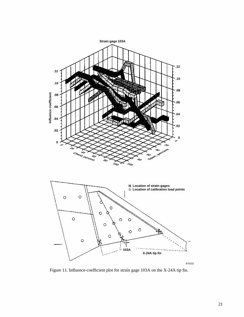
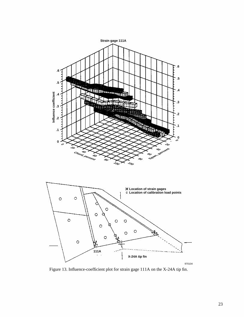
Figures 11, 12, and 13 show influence-coefficient plots that cover the range of responses seen on this structure.Figure 11 shows an influence-coefficient plot that illustrates a typical shear response. Numerous strain gagesrespond in a similar manner. Figure 12 shows the response of the strain gage that shows a sensitivity to the loadson the control surface at the rear of the structure. Figure 13 shows a response that illustrates a very specificbending effect. Numerous sensors showed a similar dominant bending effect. By inspecting the three drasticallydifferent types of responses of the individual strain gages of figure 14, the linear combining of the gages falls shortof the flat response required for a well-defined shear equation.
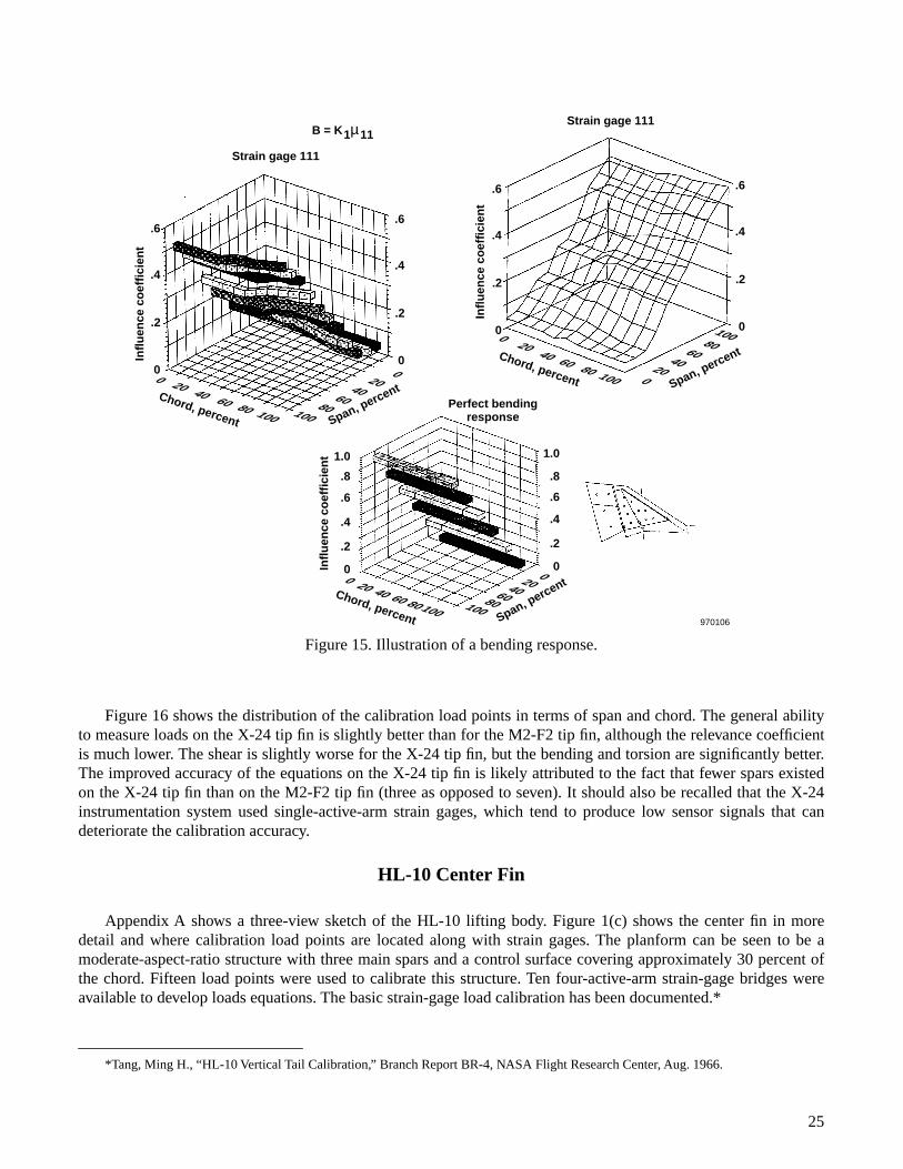
Figure 15 shows a strain gage that exhibits a very good characteristic in terms of sensing bending moment. The“perfect” bending response is shown as a ribbon plot along with the ribbon plot of the actual strain gage (SG 111).The wire-frame plot is introduced as another tool to look at the influence-coefficient plots. The wire-framesoftware plots the span values opposite to the ribbon plot, providing a reverse way of looking at the data.
The best equations that could be developed resulted in load measurements with the following estimated errors:
The 16 load points used in the calibration resulted in the following relevance coefficient:
*DeAngelis, V. Michael, “X-24A Loads Calibration,” Branch Report BR-26, NASA Flight Research Center, 1968.
Shear 11 percent
Bending Moment 7 percent
Torsion 18 percent
CR 0.49=
19
20
0 10 20 30 40 50Span, percent
60 70 80 90 100
0 10 20 30 40 50Chord, percent
60 70 80 90 100
970101
8
6
4Numberof loadpoints
2
12
10
8
6Numberof loadpoints
2
4
0
0
Figure 10. Distribution of load points in the span and chord directions for the M2-F2 tip fin.
21
Strain gage 103A
.12
.10
.08
.06
.04
.02
0
.12
Infl
uen
ce c
oef
fici
ent
.10
.08
.06
.04
.02
0
100
Chord, percent Span, percent
100
8080
6060
4040
2020
00
Location of strain gagesLocation of calibration load points
103AX-24A tip fin
970102
Figure 11. Influence-coefficient plot for strain gage 103A on the X-24A tip fin.

22
Strain gage 106A
.12
.14
.16
Infl
uen
ce c
oef
fici
ent
.10
.08
.06
.04
.02
0
.12
.14
.16
.10
.08
.06
.04
.02
0
100
Chord, percent Span, percent
100
8080
6060
4040
20
200
Location of strain gagesLocation of calibration load points
106AX-24A tip fin
970103
Figure 12. Influence-coefficient plot for strain gage 106A on the X-24A tip fin.
23
Strain gage 111A
.6
.5
.4
.3
.2
.1
0
.6
Infl
uen
ce c
oef
fici
ent
.5
.4
.3
.2
.1
0
100
Chord, percent Span, percent
100
8080
6060
4040
2020
00
Location of strain gagesLocation of calibration load points
111A
X-24A tip fin
970104
Figure 13. Influence-coefficient plot for strain gage 111A on the X-24A tip fin.

24
970105
Chord, percent Span, percent
1001008080
60604040
20200
0
0
1001008080
60604040
20200
Infl
uen
ce c
oef
fici
ent
Chord, percent Span, percent
Span, percent
Strain gage 103
Strain gage 106
V = K1µ103 + K2µ106 + K3µ111
Perfect shear response
.5
.4
.3
.2
.1
0
.5
.4
.3
.2
.1
.0
Infl
uen
ce c
oef
fici
ent
.16
.12
.08
.04
0
.16
.12
.08
.04
0
0
1001008080
60604040
20200Chord, percent Span, percent
Infl
uen
ce c
oef
fici
ent
.12
.08
.04
0
.12
.08
.04
00
1001008080
60604040
20200Chord, percent Span, percent
Infl
uen
ce c
oef
fici
ent
0
.2
.4
.6
0
.2
.4
.6
Strain gage 111
Figure 14. Illustration of how several strain gages are combined to obtain a favorable shear response.
0
1001008080
60604040
20200
10080
6040
200
Chord, percent
Chord, percent
Span, percent
0
10080
6040
20
Span, percent
Infl
uen
ce c
oef
fici
ent
Infl
uen
ce c
oef
fici
ent 1.0
.8
.6
.4
.2
0
1.0
.8
.6
.4
.2
0
.6
.4
.2
0
.6
.4
.2
0
.6
.4
.2
0
.6
.4
.2
0100
01002080
40606040
80200Chord, percent Span, percent
Infl
uen
ce c
oef
fici
ent
Strain gage 111
Strain gage 111
Perfect bendingresponse
B = K1µ11
970106
Figure 15. Illustration of a bending response.
Figure 16 shows the distribution of the calibration load points in terms of span and chord. The general abilityto measure loads on the X-24 tip fin is slightly better than for the M2-F2 tip fin, although the relevance coefficientis much lower. The shear is slightly worse for the X-24 tip fin, but the bending and torsion are significantly better.The improved accuracy of the equations on the X-24 tip fin is likely attributed to the fact that fewer spars existedon the X-24 tip fin than on the M2-F2 tip fin (three as opposed to seven). It should also be recalled that the X-24instrumentation system used single-active-arm strain gages, which tend to produce low sensor signals that candeteriorate the calibration accuracy.
HL-10 Center Fin
Appendix A shows a three-view sketch of the HL-10 lifting body. Figure 1(c) shows the center fin in moredetail and where calibration load points are located along with strain gages. The planform can be seen to be amoderate-aspect-ratio structure with three main spars and a control surface covering approximately 30 percent ofthe chord. Fifteen load points were used to calibrate this structure. Ten four-active-arm strain-gage bridges wereavailable to develop loads equations. The basic strain-gage load calibration has been documented.*
*Tang, Ming H., “HL-10 Vertical Tail Calibration,” Branch Report BR-4, NASA Flight Research Center, Aug. 1966.
25
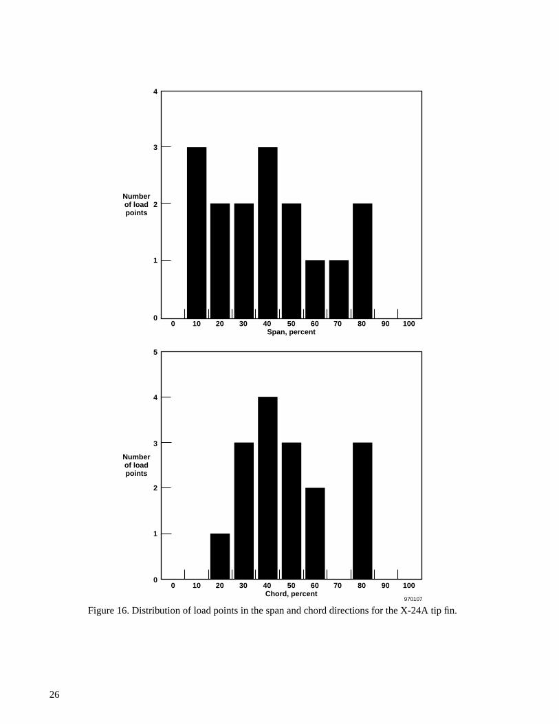
26
0 10 20 30 40 50Span, percent
60 70 80 90 100
0 10 20 30 40 50Chord, percent
60 70 80 90 100
970107
4
3
2Numberof loadpoints
1
5
4
3
2
Numberof loadpoints
1
0
0
Figure 16. Distribution of load points in the span and chord directions for the X-24A tip fin.

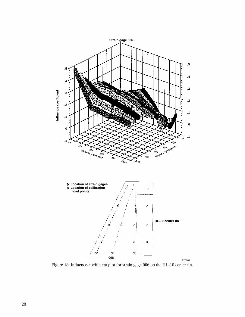
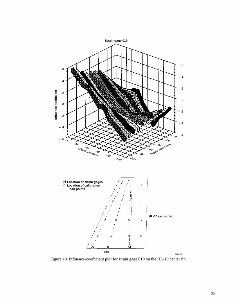
The HL-10 center fin has a large, slim planform; hence, the problems associated with very low-aspect-ratiostructures should not be present. All 10 strain-gage bridges were sensitive to some degree to both bending andtorsion. Figures 17, 18, and 19 show as ribbon plots the responses of 3 strain-gage bridges that are characteristic ofthe group of 10. Figure 17 shows the strain-gage bridge located on the center spar, and the response is largely abending one. Figure 18 shows a strain-gage bridge also located on the center spar. The dominant response of thisbridge is shear with bending and torsion contaminants. Figure 19 shows a strain-gage bridge located on the aftspar. This bridge responds largely to torsion with some bending contamination.
27
Strain gage 004
.6
Infl
uen
ce c
oef
fici
ent
.4
.2
0
– .2
– .4
.6
.4
.2
0
– .2
– .4
100
Chord, percent Span, percent
100
8080
6060
4040
2020
00
Location of strain gagesLocation of calibration load points
004
HL-10 center fin
970108
Figure 17. Influence-coefficient plot for strain gage 004 on the HL-10 center fin.
28
Strain gage 006
.5
.4
.3
.2
.1
0
– .1
.5
.4
.3
.2
.1
0
– .1
Infl
uen
ce c
oef
fici
ent
100
Chord, percent Span, percent
100
8080
6060
4040
2020
00
Location of strain gagesLocation of calibration load points
006
HL-10 center fin
970109
Figure 18. Influence-coefficient plot for strain gage 006 on the HL-10 center fin.
29
Strain gage 010
.6
.4
.2
0
– .2
– .4
– .6
.6
.4
.2
0
– .2
– .4
– .6
Infl
uen
ce c
oef
fici
ent
100
Chord, percent Span, percent
100
8080
6060
4040
2020
00
Location of strain gagesLocation of calibration load points
010
HL-10 center fin
970110
Figure 19. Influence-coefficient plot for strain gage 010 on the HL-10 center fin.
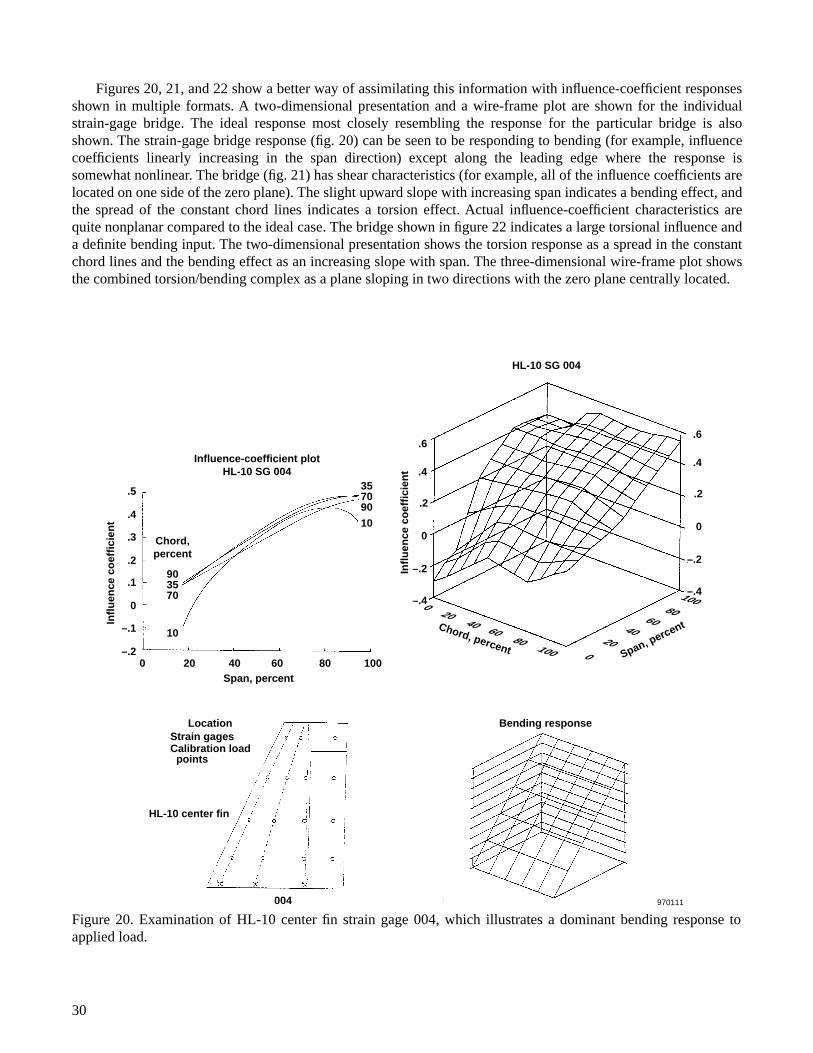
Figures 20, 21, and 22 show a better way of assimilating this information with influence-coefficient responsesshown in multiple formats. A two-dimensional presentation and a wire-frame plot are shown for the individualstrain-gage bridge. The ideal response most closely resembling the response for the particular bridge is alsoshown. The strain-gage bridge response (fig. 20) can be seen to be responding to bending (for example, influencecoefficients linearly increasing in the span direction) except along the leading edge where the response issomewhat nonlinear. The bridge (fig. 21) has shear characteristics (for example, all of the influence coefficients arelocated on one side of the zero plane). The slight upward slope with increasing span indicates a bending effect, andthe spread of the constant chord lines indicates a torsion effect. Actual influence-coefficient characteristics arequite nonplanar compared to the ideal case. The bridge shown in figure 22 indicates a large torsional influence anda definite bending input. The two-dimensional presentation shows the torsion response as a spread in the constantchord lines and the bending effect as an increasing slope with span. The three-dimensional wire-frame plot showsthe combined torsion/bending complex as a plane sloping in two directions with the zero plane centrally located.
30
Figure 20. Examination of HL-10 center fin strain gage 004, which illustrates a dominant bending response toapplied load.
100
0100
20804060
60408020
0
Chord, percent Span, percent
Infl
uen
ce c
oef
fici
ent
Infl
uen
ce c
oef
fici
ent
.6
.4
.2
0
–.2
–.4
.6
.4
.2
0
–.2
–.4
HL-10 SG 004
HL-10 center fin
004
Bending responseLocationStrain gagesCalibration load points
970111
Chord,percent
Span, percent
Influence-coefficient plotHL-10 SG 004
903570
357090
10
10
0
.5
.4
.3
.2
.1
0
–.1
–.220 40 80 10060

31
0
10080
6040
20Chord, percent
100
020
4060
80
Span, percent
Infl
uen
ce c
oef
fici
ent
.5
.4
.3
.2
.1
0
.5
.4
.3
.2
.1
0
HL-10 center fin
006
Shear with torsion/bending
LocationStrain gagesCalibration load points
970112
Influence-coefficient plotHL-10 SG 006
Chord,percent
357010
357090
Infl
uen
ce c
oef
fici
ent .5
.4
.3
.2
.1
0
90
10
Span, percent20 40 80 10060
HL-10 SG 006
Figure 21. Examination of HL-10 center fin strain gage 006, which illustrates an example of a shear response withtorsion and bending superimposed.

0
10080
6040
20Chord, percent
100
020
4060
80
Span, percent
Infl
uen
ce c
oef
fici
ent
.6
.4
.2
0
–.2
–.4
.6
.4
.2
0
–.2
–.4
HL-10 center fin
010
Bending/torsion response
LocationStrain gages Calibration load points
970113
Influence-coefficient plot HL-10 SG 010
Chord, percent
Infl
uen
ce c
oef
fici
ent
.4
.3
.2
.1
0
–.1
–.2
–.3
–.4
–.5
10
35
90
70
70
90
35
10
Span, percent0 20 40 80 10060
HL-10 SG 010
Figure 22. Examination of HL-10 center fin strain gage 010, which illustrates an example of a response with strongtorsion and bending characteristics.
The best equations that could be developed resulted in load measurements with the following estimated errors:
The 16 load points used in calibrating the strain-gage bridges on this structure resulted in a fairly largerelevance coefficient:
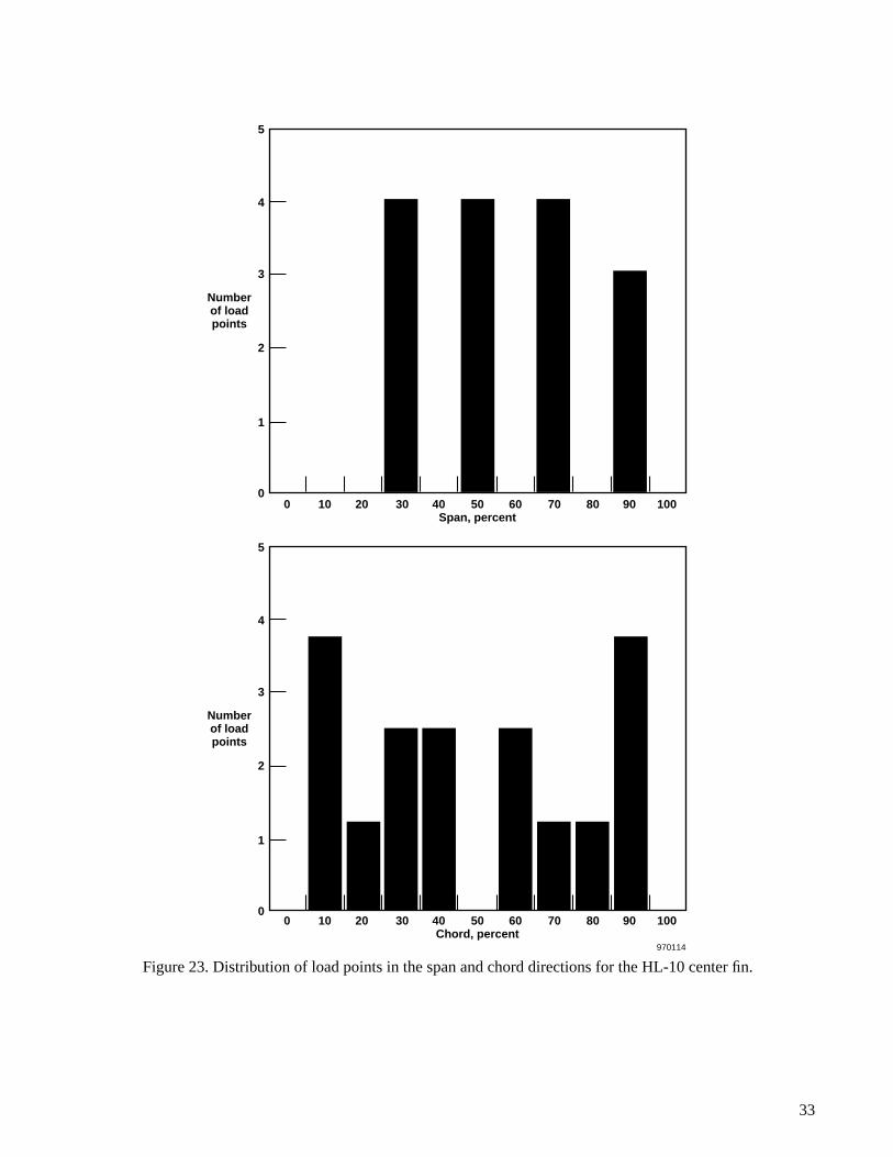
Figure 23 shows the distribution of the calibration load points in terms of span and chord. The relatively goodstrain-gage calibration is attributable to several favorable circumstances. The large aspect ratio of a lifting andstabilizing structure provides a favorable geometry for a good calibration. The strain-gage bridge outputs werefairly large, which eliminates resolution problems. A relevance coefficient of 0.60 results in a favorable loadingdistribution.
Shear 10 percent
Bending Moment 6 percent
Torsion 16 percent
CR 0.60=
32
33
5
4
3
2
Numberof loadpoints
1
0
5
4
3
2
Numberof loadpoints
1
00 10 20 30 40 50
Chord, percent60 70 80 90 100
0 10 20 30 40 50Span, percent
60 70 80 90 100
970114
Figure 23. Distribution of load points in the span and chord directions for the HL-10 center fin.
X-24 Center Fin
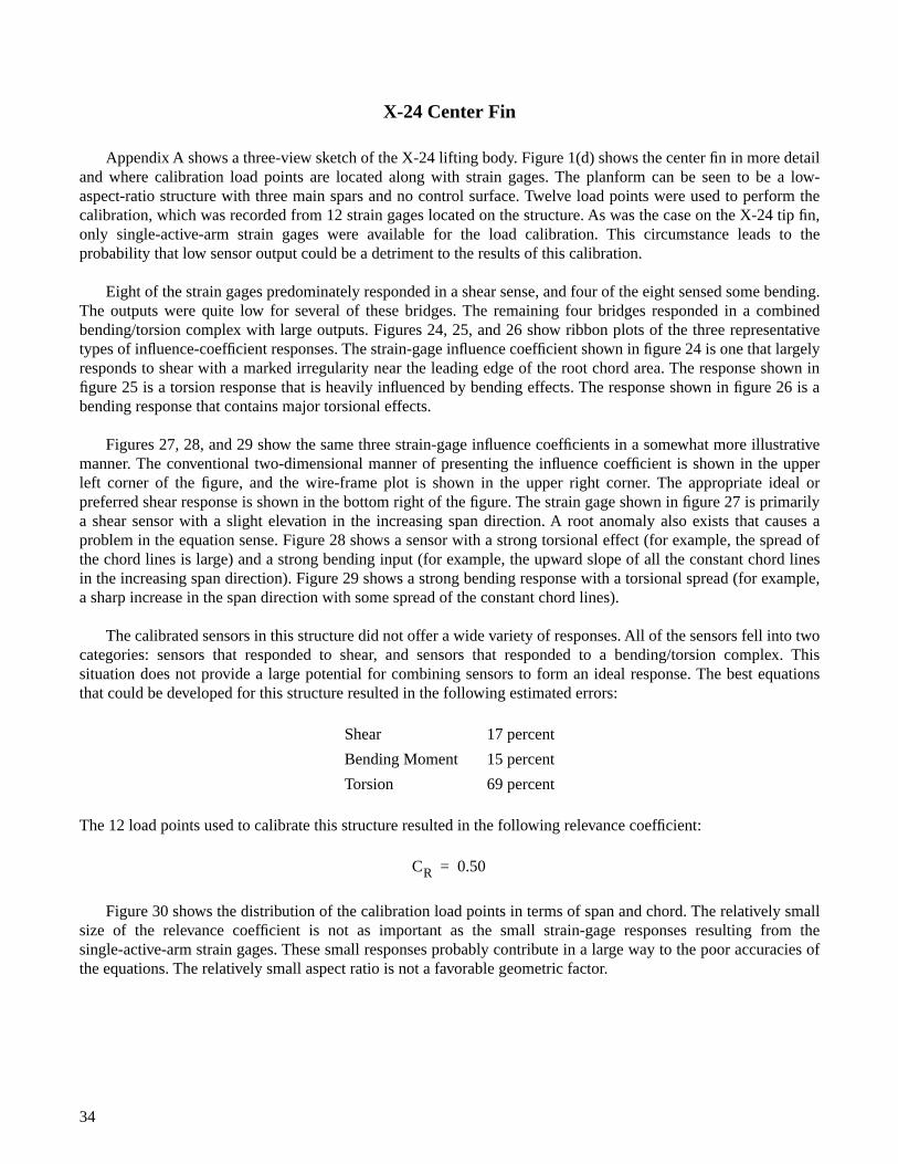
Appendix A shows a three-view sketch of the X-24 lifting body. Figure 1(d) shows the center fin in more detailand where calibration load points are located along with strain gages. The planform can be seen to be a low-aspect-ratio structure with three main spars and no control surface. Twelve load points were used to perform thecalibration, which was recorded from 12 strain gages located on the structure. As was the case on the X-24 tip fin,only single-active-arm strain gages were available for the load calibration. This circumstance leads to theprobability that low sensor output could be a detriment to the results of this calibration.
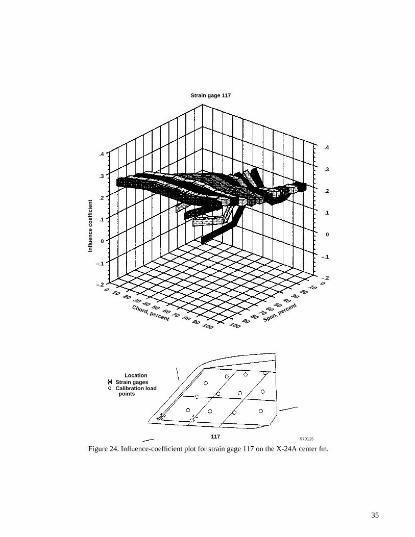
Eight of the strain gages predominately responded in a shear sense, and four of the eight sensed some bending.The outputs were quite low for several of these bridges. The remaining four bridges responded in a combinedbending/torsion complex with large outputs. Figures 24, 25, and 26 show ribbon plots of the three representativetypes of influence-coefficient responses. The strain-gage influence coefficient shown in figure 24 is one that largelyresponds to shear with a marked irregularity near the leading edge of the root chord area. The response shown infigure 25 is a torsion response that is heavily influenced by bending effects. The response shown in figure 26 is abending response that contains major torsional effects.
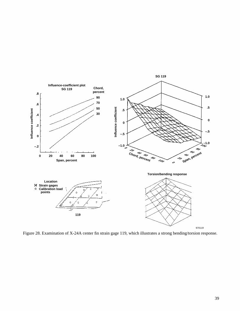
Figures 27, 28, and 29 show the same three strain-gage influence coefficients in a somewhat more illustrativemanner. The conventional two-dimensional manner of presenting the influence coefficient is shown in the upperleft corner of the figure, and the wire-frame plot is shown in the upper right corner. The appropriate ideal orpreferred shear response is shown in the bottom right of the figure. The strain gage shown in figure 27 is primarilya shear sensor with a slight elevation in the increasing span direction. A root anomaly also exists that causes aproblem in the equation sense. Figure 28 shows a sensor with a strong torsional effect (for example, the spread ofthe chord lines is large) and a strong bending input (for example, the upward slope of all the constant chord linesin the increasing span direction). Figure 29 shows a strong bending response with a torsional spread (for example,a sharp increase in the span direction with some spread of the constant chord lines).
The calibrated sensors in this structure did not offer a wide variety of responses. All of the sensors fell into twocategories: sensors that responded to shear, and sensors that responded to a bending/torsion complex. Thissituation does not provide a large potential for combining sensors to form an ideal response. The best equationsthat could be developed for this structure resulted in the following estimated errors:
The 12 load points used to calibrate this structure resulted in the following relevance coefficient:
Figure 30 shows the distribution of the calibration load points in terms of span and chord. The relatively smallsize of the relevance coefficient is not as important as the small strain-gage responses resulting from thesingle-active-arm strain gages. These small responses probably contribute in a large way to the poor accuracies ofthe equations. The relatively small aspect ratio is not a favorable geometric factor.
Shear 17 percent
Bending Moment 15 percent
Torsion 69 percent
CR 0.50=
34
35
Strain gage 117
117 970115
Chord, percent Span, percent
100100
80909080
6050
7060 70
4040
1020302010
3050
00
Infl
uen
ce c
oef
fici
ent
.4
.3
.2
.1
0
–.1
–.2
.4
.3
.2
.1
0
–.1
–.2
LocationStrain gages Calibration load points
Figure 24. Influence-coefficient plot for strain gage 117 on the X-24A center fin.
36
Strain gage 119
119970116
Chord, percent Span, percent
100100
80909080
6050
7060 70
4040
1020302010
3050
00
Infl
uen
ce c
oef
fici
ent
1.0
.5
0
–.5
–1.0
LocationStrain gages Calibration load points
1.0
.5
0
–.5
–1.0
Figure 25. Influence-coefficient plot for strain gage 119 on the X-24A center fin.

37
Strain gage 124
124 970117
Chord, percent Span, percent
100100
80909080
6050
7060 70
4040
1020302010
3050
00
Infl
uen
ce c
oef
fici
ent
LocationStrain gages Calibration load points
1.0
.8
.4
.6
.2
0
–.2
1.0
.8
.4
.6
.2
0
–.2
Figure 26. Influence-coefficient plot for strain gage 124 on the X-24A center fin.

38
0
10080
6040
20Chord, percent
100
020
4060
80
Span, percent
Infl
uen
ce c
oef
fici
ent
.4
.3
.2
.1
0
–.1
117
X-24 center fin
Shear response
SG 117
.4
.3
.2
.1
0
–.1
LocationStrain gages Calibration load points
970118
Influence-coefficient plot SG 117
Chord, percent
Infl
uen
ce c
oef
fici
ent
.4
.2
0
90
70
30
50
Span, percent20 40 80 10060
Figure 27. Examination of X-24A center fin strain gage 117, which illustrates a strong shear response.
39
100
0100
20804060
60408020
0
Chord, percent Span, percent
Infl
uen
ce c
oef
fici
ent
Infl
uen
ce c
oef
fici
ent
1.0
.5
0
–.5
–1.0
SG 119
119
Torsion/bending response
LocationStrain gages Calibration load points
970119
Chord, percent
Span, percent
Influence-coefficient plot SG 119
90
70
50
30
0
.6
.4
.2
0
.8
20 40 80 10060
1.0
.5
0
–.5
–1.0–.2
Figure 28. Examination of X-24A center fin strain gage 119, which illustrates a strong bending/torsion response.

40
100
0100
20804060
60408020
0
Chord, percent Span, percent
Infl
uen
ce c
oef
fici
ent
Infl
uen
ce c
oef
fici
ent
SG 124
124
Bending response
LocationStrain gages Calibration load points
970120
Chord, percent
Span, percent
Influence-coefficient plot SG 124
90
70
50
30
0
.6
.4
.2
0
–.2
.8
20 40 80 10060
1.0
.8
.6
.4
.2
0
1.0
.8
.6
.4
.2
0
Figure 29. Examination of X-24A center fin strain gage 124, which illustrates a strong bending response.

41
4
3
2Numberof loadpoints
1
00 10 20 30 40 50
Span, percent60 70 80 90 100
4
3
2Numberof loadpoints
1
00 10 20 30 40 50
Chord, percent60 70 80 90 100
970121
Figure 30. Distribution of load points in the span and chord directions for the X-24A center fin.
X-15 Horizontal Tail
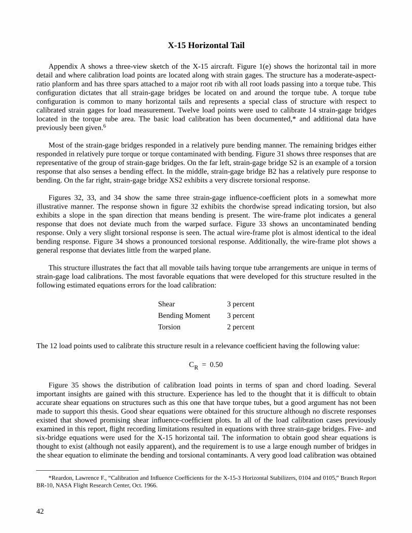
Appendix A shows a three-view sketch of the X-15 aircraft. Figure 1(e) shows the horizontal tail in moredetail and where calibration load points are located along with strain gages. The structure has a moderate-aspect-ratio planform and has three spars attached to a major root rib with all root loads passing into a torque tube. Thisconfiguration dictates that all strain-gage bridges be located on and around the torque tube. A torque tubeconfiguration is common to many horizontal tails and represents a special class of structure with respect tocalibrated strain gages for load measurement. Twelve load points were used to calibrate 14 strain-gage bridgeslocated in the torque tube area. The basic load calibration has been documented,* and additional data havepreviously been given.6
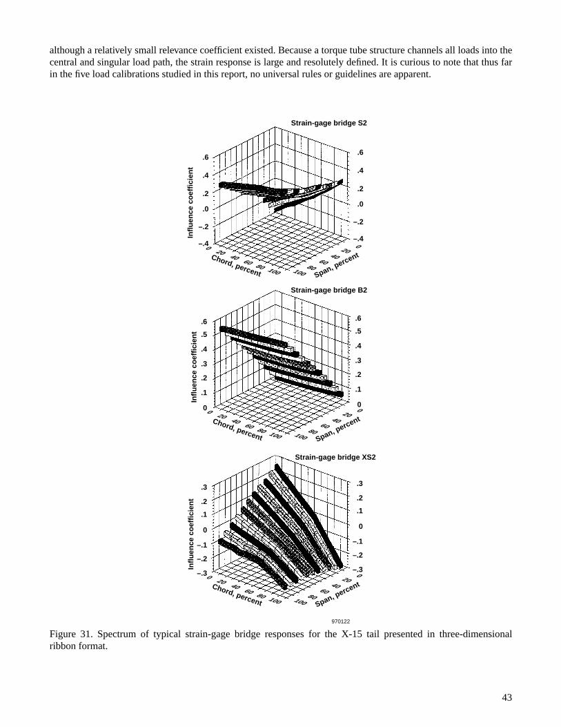
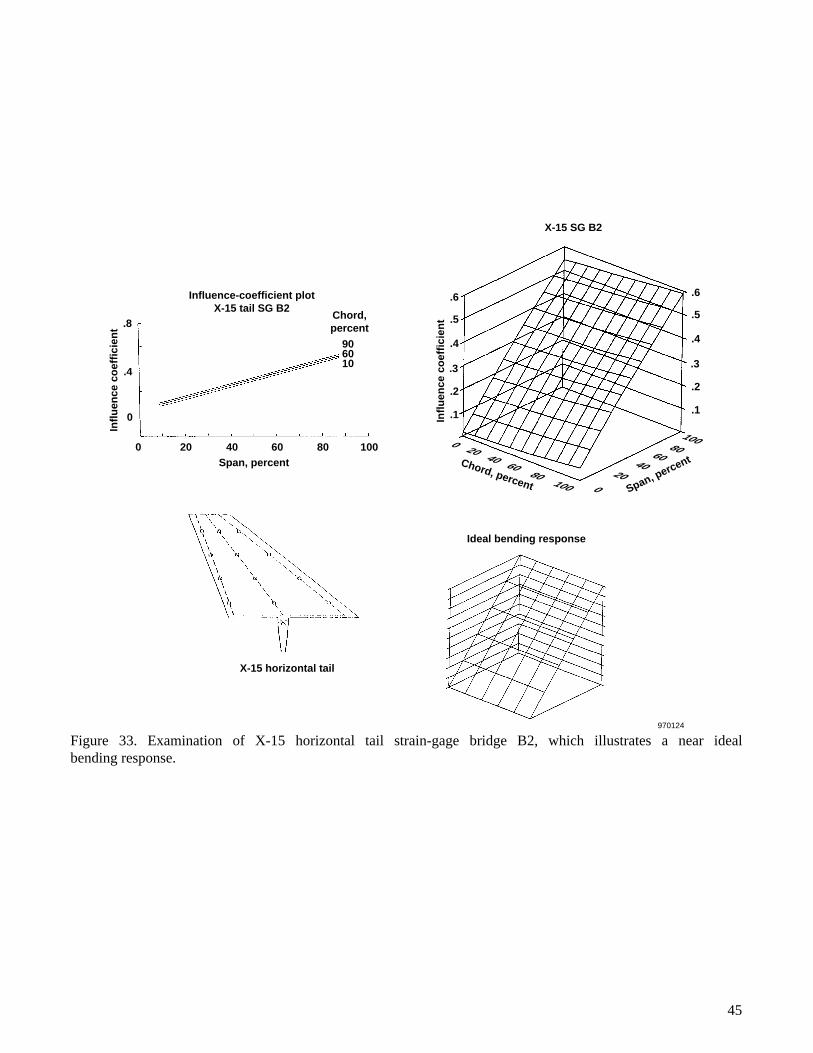
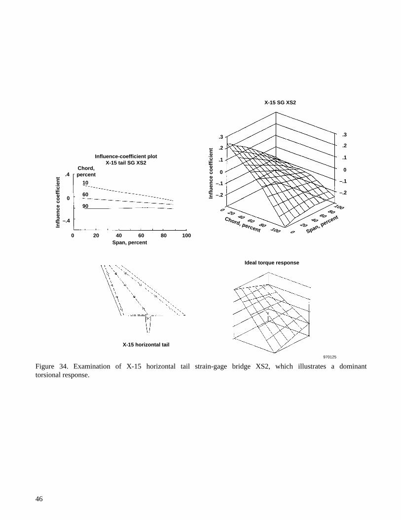
Most of the strain-gage bridges responded in a relatively pure bending manner. The remaining bridges eitherresponded in relatively pure torque or torque contaminated with bending. Figure 31 shows three responses that arerepresentative of the group of strain-gage bridges. On the far left, strain-gage bridge S2 is an example of a torsionresponse that also senses a bending effect. In the middle, strain-gage bridge B2 has a relatively pure response tobending. On the far right, strain-gage bridge XS2 exhibits a very discrete torsional response.
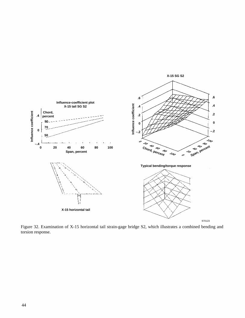
Figures 32, 33, and 34 show the same three strain-gage influence-coefficient plots in a somewhat moreillustrative manner. The response shown in figure 32 exhibits the chordwise spread indicating torsion, but alsoexhibits a slope in the span direction that means bending is present. The wire-frame plot indicates a generalresponse that does not deviate much from the warped surface. Figure 33 shows an uncontaminated bendingresponse. Only a very slight torsional response is seen. The actual wire-frame plot is almost identical to the idealbending response. Figure 34 shows a pronounced torsional response. Additionally, the wire-frame plot shows ageneral response that deviates little from the warped plane.
This structure illustrates the fact that all movable tails having torque tube arrangements are unique in terms ofstrain-gage load calibrations. The most favorable equations that were developed for this structure resulted in thefollowing estimated equations errors for the load calibration:
The 12 load points used to calibrate this structure result in a relevance coefficient having the following value:
Figure 35 shows the distribution of calibration load points in terms of span and chord loading. Severalimportant insights are gained with this structure. Experience has led to the thought that it is difficult to obtainaccurate shear equations on structures such as this one that have torque tubes, but a good argument has not beenmade to support this thesis. Good shear equations were obtained for this structure although no discrete responsesexisted that showed promising shear influence-coefficient plots. In all of the load calibration cases previouslyexamined in this report, flight recording limitations resulted in equations with three strain-gage bridges. Five- andsix-bridge equations were used for the X-15 horizontal tail. The information to obtain good shear equations isthought to exist (although not easily apparent), and the requirement is to use a large enough number of bridges inthe shear equation to eliminate the bending and torsional contaminants. A very good load calibration was obtained
*Reardon, Lawrence F., “Calibration and Influence Coefficients for the X-15-3 Horizontal Stabilizers, 0104 and 0105,” Branch ReportBR-10, NASA Flight Research Center, Oct. 1966.
Shear 3 percent
Bending Moment 3 percent
Torsion 2 percent
CR 0.50=
42
although a relatively small relevance coefficient existed. Because a torque tube structure channels all loads into thecentral and singular load path, the strain response is large and resolutely defined. It is curious to note that thus farin the five load calibrations studied in this report, no universal rules or guidelines are apparent.
43
Strain-gage bridge XS2
Strain-gage bridge B2
Strain-gage bridge S2
970122
Chord, percent Span, percent
1001008080
60604040
202000
Infl
uen
ce c
oef
fici
ent
–.3
–.2
–.1
0
.1
.2
.3
Chord, percent Span, percent
1001008080
60604040
202000
Chord, percent Span, percent
1001008080
60604040
202000
Infl
uen
ce c
oef
fici
ent .5
.6
.4
.3
.2
.1
0
Infl
uen
ce c
oef
fici
ent
.6
.4
.2
.0
–.2
–.4
.6
.4
.2
.0
–.2
–.4
.5
.6
.4
.3
.2
.1
0
–.3
–.2
–.1
0
.1
.2
.3
Figure 31. Spectrum of typical strain-gage bridge responses for the X-15 tail presented in three-dimensionalribbon format.
44
100
01002080
40606040
80200
Chord, percent Span, percent
Infl
uen
ce c
oef
fici
ent
Infl
uen
ce c
oef
fici
ent
X-15 SG S2
X-15 horizontal tail
Typical bending/torque response
970123
Chord, percent
Span, percent
Influence-coefficient plot X-15 tail SG S2
90
70
50
0
.4
0
–.480 100604020
.6
.4
.2
–.2
0
.6
.4
.2
–.2
0
Figure 32. Examination of X-15 horizontal tail strain-gage bridge S2, which illustrates a combined bending andtorsion response.
45
100
01002080
40606040
80200
Chord, percent Span, percent
Infl
uen
ce c
oef
fici
ent
Infl
uen
ce c
oef
fici
ent
X-15 SG B2
X-15 horizontal tail
Ideal bending response
970124
Chord, percent
Span, percent
Influence-coefficient plot X-15 tail SG B2
906010
0
.8
.4
0
80 100604020
.6
.5
.4
.2
.1
.3
.6
.5
.4
.2
.1
.3
Figure 33. Examination of X-15 horizontal tail strain-gage bridge B2, which illustrates a near idealbending response.
46
100
01002080
40606040
80200
Chord, percent Span, percentIn
flu
ence
co
effi
cien
t
Infl
uen
ce c
oef
fici
ent
X-15 SG XS2
X-15 horizontal tail
Ideal torque response
970125
Chord, percent
Span, percent
Influence-coefficient plot X-15 tail SG XS2
90
60
10
0
.4
0
–.4
80 100604020
.3
.2
.1
–.1
–.2
0
.3
.2
.1
–.1
–.2
0
Figure 34. Examination of X-15 horizontal tail strain-gage bridge XS2, which illustrates a dominanttorsional response.

47
4
3
2Numberof loadpoints
1
0
5
4
3
2
Numberof loadpoints
1
00 10 20 30 40 50
Chord, percent60 70 80 90 100
0 10 20 30 40 50Span, percent
60 70 80 90 100
970126
Figure 35. Distribution of load points in the span and chord directions for the X-15 horizontal tail.

F-89 Wing
Appendix A shows a three-view sketch of the F-89 aircraft. Figure 1(f) shows the wing in more detail andwhere calibration load points are located along with strain-gage bridges. The structure is of a straight-wingconfiguration with a moderate-aspect-ratio planform with five primary spars. Major control surfaces are located atthe aft of the wing. Thirty load points were used to calibrate the strain gages located near the root of the five spars.This structure was not a NASA-calibrated structure but is included because it is the first example of the extensiveapplication of reference 1. The detail has been documented in partial form.* A table of primary influencecoefficients is not available.
This structure is included in this report because of the historic timing of the calibration, and because itrepresents a case where the subject of nonlinearity can be introduced. The influence-coefficient plot for straingage 62 is shown in the upper left corner of figure 36. The locations of the load points and the root strain gages(including 62) are shown at the upper right. This structure was not loaded aft of the 62-percent chord; therefore,approximately the aft 40 percent of the structure was not loaded. The inboard 20 percent was also not loaded. Thisstructure presents a case where large areas of the structure are not directly loaded. This case requires extensiveextrapolation to develop a linear equation that defines the response of strain gage 62 to discrete loads over theentire wing surface. A minimum of three methods of extrapolating the load calibration were used: linearextrapolation, extrapolation of the last two points, and nonlinear curve fitting. The left bottom of figure 36 shows
*Gray, A. K. J., “Procedures Manual for Flight Test Determination and Evaluation of Load Distribution and Structural Integrity,” ReportNo. EFT-55-1, Northrop Aircraft, Inc., June 1955.
48
Infl
uen
ce c
oef
fici
ent,
ou
tpu
t/lb
f
970127
Chord,percent
Span, percent
Strain gage
60
50402510
Chord,percent
General fairing Extrapolationoflast two points
Nonlinearextrapolation
6050402510
Chord,percent
6050402510
Chord,percent
6050402510
2400 x 10 – 6
1600
800
0
– 800
Infl
uen
ce c
oef
fici
ent,
ou
tpu
t/lb
f
2400 x 10 – 6
1600
800
0
– 800
1000 20 40 60 80
Span, percent1000 20 40 60 80
Span, percent1000 20 40 60 80
Span, percent1000 20 40 60 80
LocationStrain gagesCalibration load points
Figure 36. General load calibration characteristics of strain gage 62 on the F-89 wing.
how a linear regression would extrapolate for values to a maximum 60-percent chord. If the two inboard loadcalibration stations were used, then the two most inboard load points, shown in the bottom middle of the figure,would be used to project the extrapolation. The third approach, shown at the bottom right, is the full curve fit,which would be used to develop a nonlinear approximation and extrapolation.
The significance of these three comparisons is typically illustrated by examining the zero-span intercept. Theload points at the 20-percent span location do not seem to follow the trend of the other load points for constantchord values. In other words, as the load points get closer to the location of the strain gages, local anomalies beginto appear in the data near the root of the lifting surface. The three methods of extrapolation shown at the bottom offigure 36 illustrate the importance of representing the extrapolation in an appropriate manner.
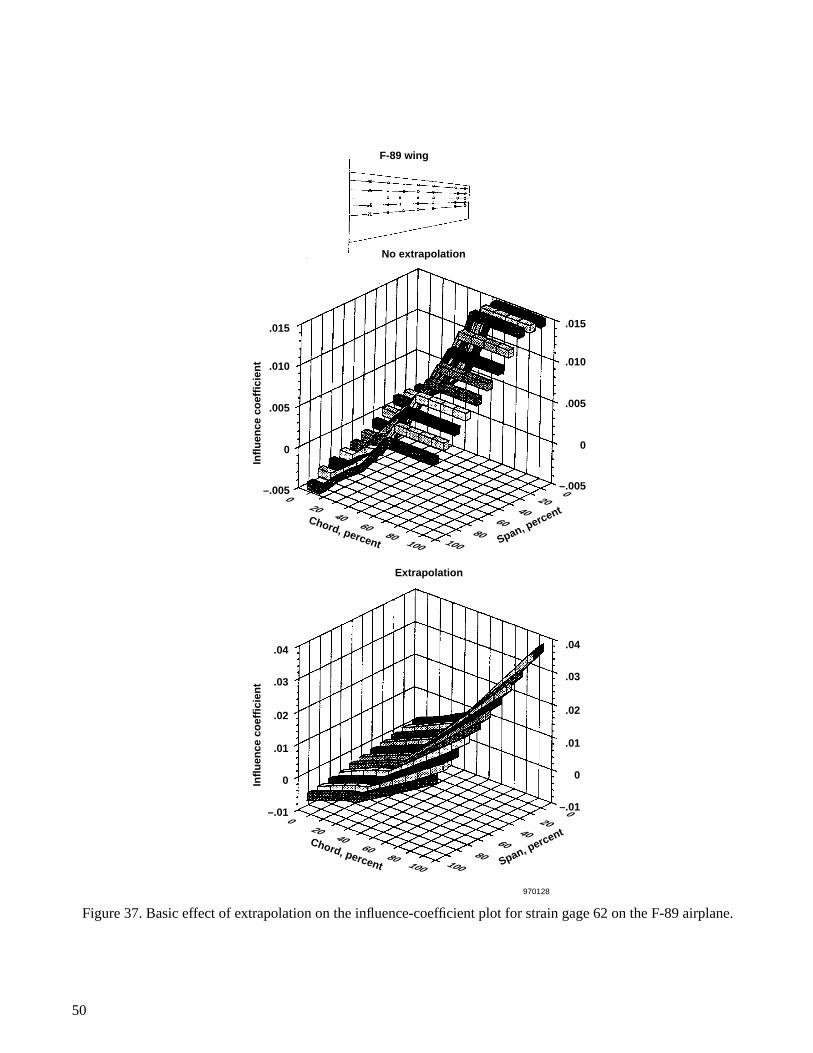
Figure 37 shows insight into the overall span/chord extrapolation relationship for strain gage 62. In the casewith no extrapolation (top ribbon plot), the curved areas represent the basic load calibration. The values at theboundaries of the calibration loads points are extended to cover 100 percent of the wing (seen as the flat areas inthe figure). In the case with extrapolation (bottom ribbon plot), the curved areas represent the basic loadcalibration. The extrapolation shown in the bottom right side of the figure consisted of extrapolating the data fromthe last two points in the chord and span directions. The extrapolation appears to minimize the actual extent of theload calibration data (fig. 37). This minimization means that the method and the extent of the extrapolation havefar-reaching impact on the equations defining loads.
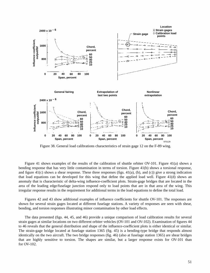
Figure 38 shows an even more extreme case, where the results of strain gage 12 are presented. The results canbe seen to diverge at and about the 20-percent span area. The zero-span intercept varies widely, and the feasibilityof applying a nonlinear curve fit as the extrapolation approach to the 50- and 60-percent chord lines seems apoor option.
This phenomenon in the area of the wing root will be seen later in the calibrations of the structures of otherwings. The phenomenon is important, and the actual mechanism has a great impact on load calibrations and theresulting equations.
The F-89 wing was calibrated with 30 load points, but because of the distribution of the spars, the relevancecoefficient was small:
Figure 39 shows the distribution of the calibration load points in terms of span and chord.
Space Shuttle Orbiter
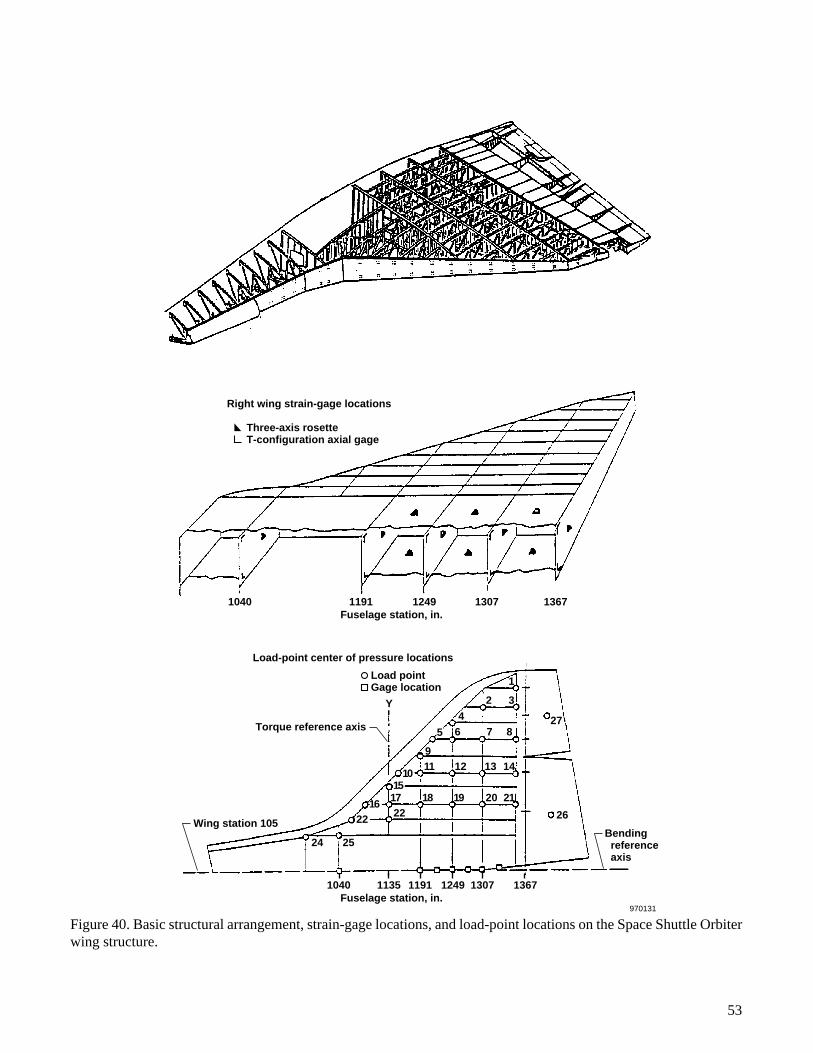
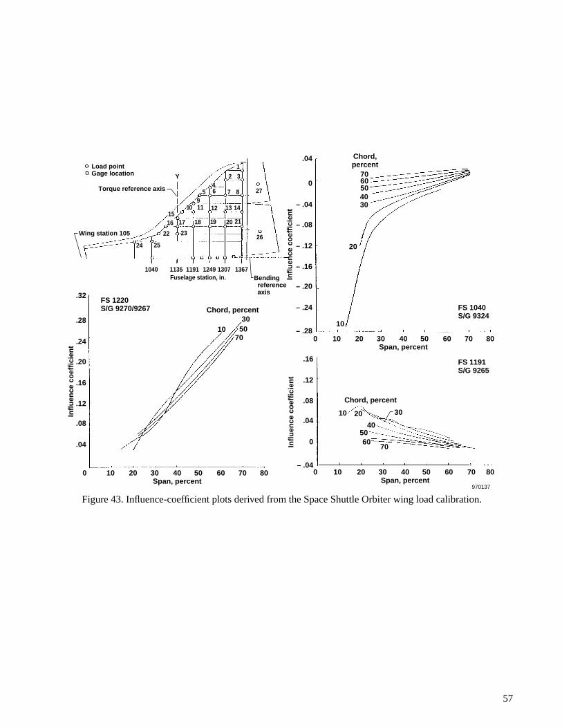
Appendix A shows a three-view sketch of the space shuttle orbiter. Figure 1(g) shows the wing in more detailand where calibration load points are located along with strain-gage bridges. The wing structure has a low-aspect-ratio planform with multiple spars that have corrugated webs and ribs that are trusses. The wing structure has largeelevons at the trailing edge and a large fairing merging with the forward fuselage. Figure 40 shows the wingstructure along with general strain-gage bridge locations. Twenty-seven load points were used to calibrate thisstructure at the locations shown (fig. 40). The shuttle orbiter wing is typical of a low-aspect-ratio delta-wingaircraft in that multiple spars and ribs are present along with a landing gear embedded in the wing. The wing alsohas control surfaces along the rear of the structure. Sufficient resources were available to complete a credible loadcalibration*† with sufficient instrumentation available. In addition, the calibration results for two shuttle orbiteraircraft (designated OV-101 and OV-102) will be presented in this section.
*Carter, A. L., “OV-101 Strain Gage Calibration for Flight Load Measurement,” Memorandum to Aerostructures Files, NASA FlightResearch Center, Apr. 1977.
†Carter, A. L., “OV-102 Wing Calibration Results,” Memorandum to Aerostructures Branch Files, NASA Flight Research Center,Oct. 1978.
CR 0.49=
49
50
F-89 wing
No extrapolation
Extrapolation
970128
Chord, percent Span, percent
1001008080
6060
4040
2020
00
Infl
uen
ce c
oef
fici
ent
–.01
0
.01
.02
.03
.04
–.01
0
.01
.02
.03
.04
Infl
uen
ce c
oef
fici
ent
–.005
0
.005
.010
.015
Chord, percent Span, percent
1001008080
6060
4040
2020
00–.005
0
.005
.010
.015
Figure 37. Basic effect of extrapolation on the influence-coefficient plot for strain gage 62 on the F-89 airplane.
Infl
uen
ce c
oef
fici
ent,
ou
tpu
t/lb
f
970129
Chord,percent
Span, percent
Strain gage
6050402510
Chord,percent
General fairing Extrapolation oflast two points
Nonlinearextrapolation
6050402510
Chord,percent
6050402510
Chord,percent
6050402510
2400 x 10 – 6
1600
0
Infl
uen
ce c
oef
fici
ent,
ou
tpu
t/lb
f
2400 x 10 – 6
1600
800
10020 40 60 80
Span, percent0 20 40 60 10080
Span, percent0 20 40 60 10080
Span, percent0 20 40 60 10080
LocationStrain gagesCalibration load points
800
Figure 38. General load calibrations characteristics of strain gage 12 on the F-89 wing.
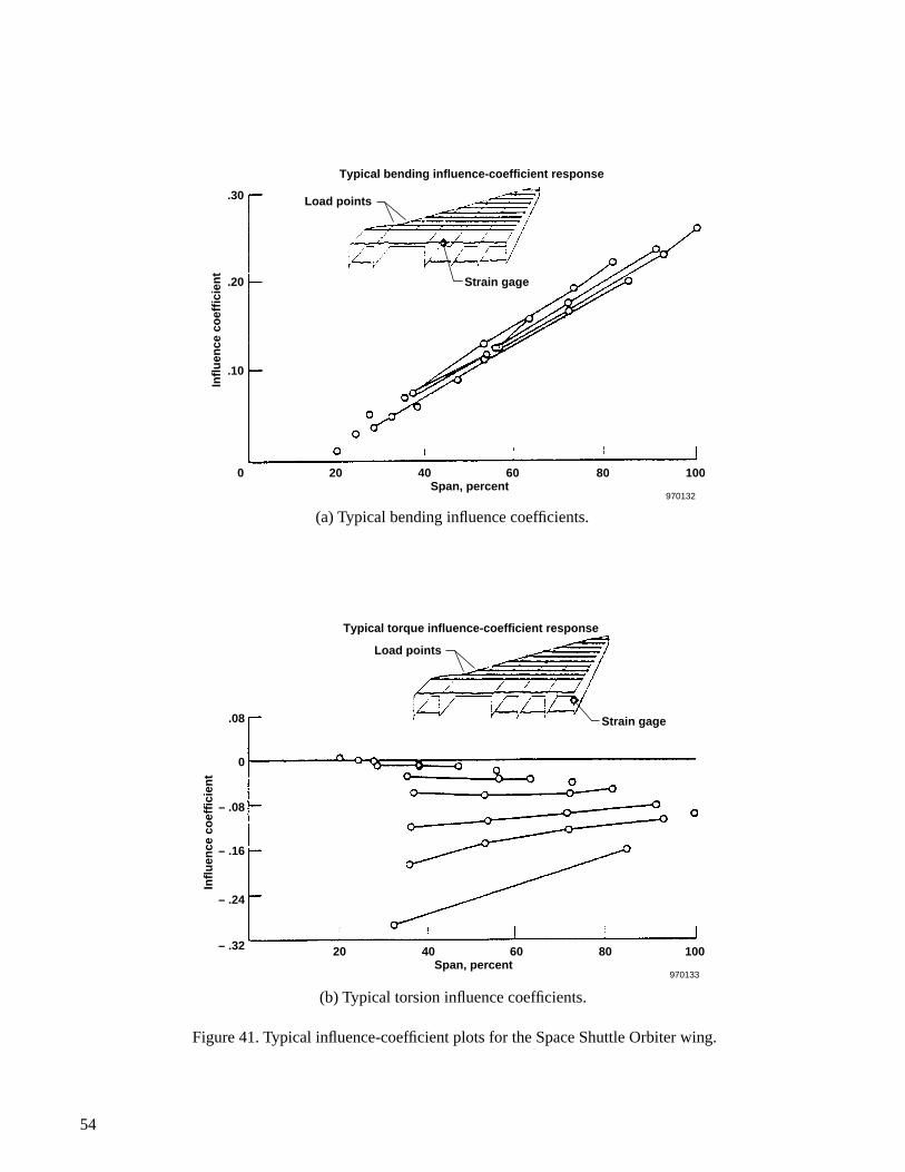
Figure 41 shows examples of the results of the calibration of shuttle orbiter OV-101. Figure 41(a) shows abending response that has very little contamination in terms of torsion. Figure 41(b) shows a torsional response,and figure 41(c) shows a shear response. These three responses (figs. 41(a), (b), and (c)) give a strong indicationthat load equations can be developed for this wing that define the applied load well. Figure 41(d) shows ananomaly that is characteristic of delta-wing influence-coefficient plots. Strain-gage bridges that are located in thearea of the leading edge/fuselage junction respond only to load points that are in that area of the wing. Thisirregular response results in the requirement for additional terms in the load equations to define the total load.
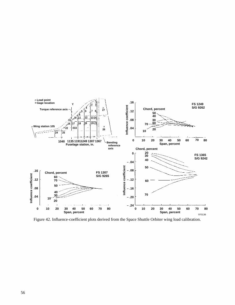
Figures 42 and 43 show additional examples of influence coefficients for shuttle OV-101. The responses areshown for several strain gages located at different fuselage stations. A variety of responses are seen with shear,bending, and torsion responses illustrating minor contamination by other load effects.
The data presented (figs. 44, 45, and 46) provide a unique comparison of load calibration results for severalstrain gages at similar locations on two different orbiter vehicles (OV-101 and OV-102). Examination of figures 44to 46 reveals that the general distribution and shape of the influence-coefficient plots is either identical or similar.The strain-gage bridge located at fuselage station 1365 (fig. 45) is a bending-type bridge that responds almostidentically on the two aircraft. The two bridge responses (fig. 46) (also at fuselage station 1365) are shear bridgesthat are highly sensitive to torsion. The shapes are similar, but a larger response exists for OV-101 thanfor OV-102.
51

52
25 50Span, percent
75 100
970130
4
3
2Numberof loadpoints
1
6
4
5
3
2
Numberof loadpoints
1
0
25 50Chord, percent
75 1000
Figure 39. Distribution of load points in the span and chord directions for the F-89 wing.
53
Right wing strain-gage locations
Load-point center of pressure locations
1191Fuselage station, in.
1249 1307
Y
27
26
1
32
46 7 8
13671040
1135Fuselage station, in.
1191 13071249 13671040
Wing station 105
Torque reference axis
Bending reference axis
Three-axis rosetteT-configuration axial gage
Load pointGage location
9
1011 12 13 14
151716
22 22
2524
18 19 20 21
970131
5
Figure 40. Basic structural arrangement, strain-gage locations, and load-point locations on the Space Shuttle Orbiterwing structure.
54
40200
.10
.20
.30 Load points
Typical bending influence-coefficient response
Infl
uen
ce c
oef
fici
ent
Strain gage
60 80 100Span, percent
970132
(a) Typical bending influence coefficients.
4020
0
– .32
– .24
– .16
– .08
.08
Load points
Typical torque influence-coefficient response
Infl
uen
ce c
oef
fici
ent
Strain gage
60 80 100Span, percent
970133
(b) Typical torsion influence coefficients.
Figure 41. Typical influence-coefficient plots for the Space Shuttle Orbiter wing.

55
0 20 40
Strain gage
Load pointsTypical shear influence-coefficient response
60Span, percent
Influencecoefficent
80 100
970134
.16
.08
0
– .08
.08
0
0 20 40
2225
24
16
Strain gage
Load point
Shear influence-coefficient for fuselage station 1040
162524
22
Fuselage station 1040
60Span, percent
Influencecoefficent
80 100
970135
– .08
– .16
– .24
– .32
(c) Typical shear influence coefficients.
(d) Complex influence-coefficient plot.
Figure 41. Concluded.
56
Load pointGage location
Torque reference axis
Wing station 105
Bending reference axis
Y
26
32
8
14
6 7
2120191817
131211
27
1367130712491191Fuselage station, in.11351040
4
1
910
1615
22
24 25
2323
5
2010 40Span, percent30 6050 80
70
70
60
50
4030
2010
.04
.08
.12
.16
0 2010 40Span, percent30 6050 80700
FS 1307S/G 9265
FS 1365S/G 9242
Infl
uen
ce c
oef
fici
ent
– .24
– .20
– .16
– .12
– .08
– .04
0
Infl
uen
ce c
oef
fici
ent
Chord, percent
2010 40Span, percent30 6050 80
70
70
60
504030
2010.04
.08
.12
.16
0
FS 1249S/G 9262
Infl
uen
ce c
oef
fici
ent
Chord, percent
70
60
50
403020
Chord, percent
970136
Figure 42. Influence-coefficient plots derived from the Space Shuttle Orbiter wing load calibration.
57
2010 40Span, percent
30 6050 80
70
70
60504030
20
10
– .04
.04
– .24
– .28
– .20
– .16
– .12
– .08
0
0
FS 1040S/G 9324
Load pointGage location
Torque reference axis
Wing station 105
Bending reference axis
Y
26
32
8
14
6 7
2120191817
131211
27
1367130712491191Fuselage station, in.11351040
Infl
uen
ce c
oef
fici
ent
Chord,percent
2010 40Span, percent
30 6050 80
70
70
5030
10
.24
.32
.04
.08
.12
.16
.20
.28
0
FS 1220S/G 9270/9267
Infl
uen
ce c
oef
fici
ent
Chord, percent
2010 40Span, percent
30 6050 80
70
70
6050
40
302010
0
– .04
.04
.08
.12
.16
0
FS 1191S/G 9265
Infl
uen
ce c
oef
fici
ent
Chord, percent
970137
4
1
59
10
1615
22
24 25
23
Figure 43. Influence-coefficient plots derived from the Space Shuttle Orbiter wing load calibration.

58
1040 1191 1249Fuselage station, in.
1307 1367
20 40 Span, percent
60 100
70
80
9050
30
10
– .010
– .015
– .005
0
.005
0
OV 102FS 1278S/G 9639In
flu
ence
co
effi
cien
t
Infl
uen
ce c
oef
fici
ent Chord, percent
20 40 Span, percent
60 100
70
80
90
5030
10
– .005
– .010
0
.005
.010
0
OV 101FS 1278S/G 9291
Chord,percent
970138
1040 1191 1249Fuselage station, in.
1307 1367
70 5030
10
OV 102FS 1365S/G 9438
Infl
uen
ce c
oef
fici
ent
Chord,percent
20 40 60Span, percent
100
70
80
50
30
10
.010
.005
.015
.020
.025
0
Infl
uen
ce c
oef
fici
ent
20 40 60Span, percent
10080
.010
.005
.015
.020
.025
0
OV 101FS 1365S/G 9334
Chord, percent
970139
Figure 44. Comparison of shear influence-coefficient plots for comparable strain-gage bridges on Space ShuttleOrbiters OV-101 and OV-102.
Figure 45. Comparison of bending influence-coefficient plots for comparable strain gage on Space Shuttle OrbitersOV-101 and OV-102.
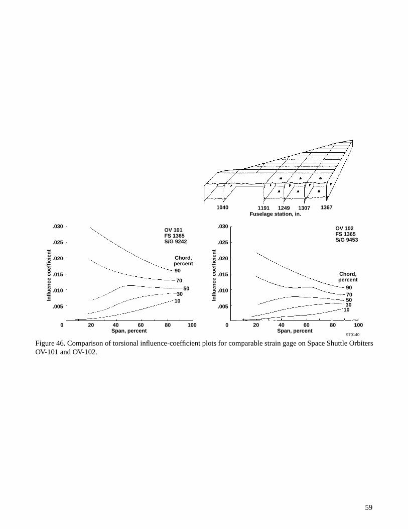
59
1040 1191 1249Fuselage station, in.
1307 1367
20 40 Span, percent
60 100
70
80
90
5030
10
.030
.025
.020
.015
.010
.005
0
OV 102FS 1365S/G 9453
Infl
uen
ce c
oef
fici
ent
20 40 Span, percent
60 10080
.030
.025
.020
.015
.010
.005
0
Infl
uen
ce c
oef
fici
ent
Chord,percent70
90
5030
10
OV 101FS 1365S/G 9242
Chord,percent
970140
Figure 46. Comparison of torsional influence-coefficient plots for comparable strain gage on Space Shuttle OrbitersOV-101 and OV-102.
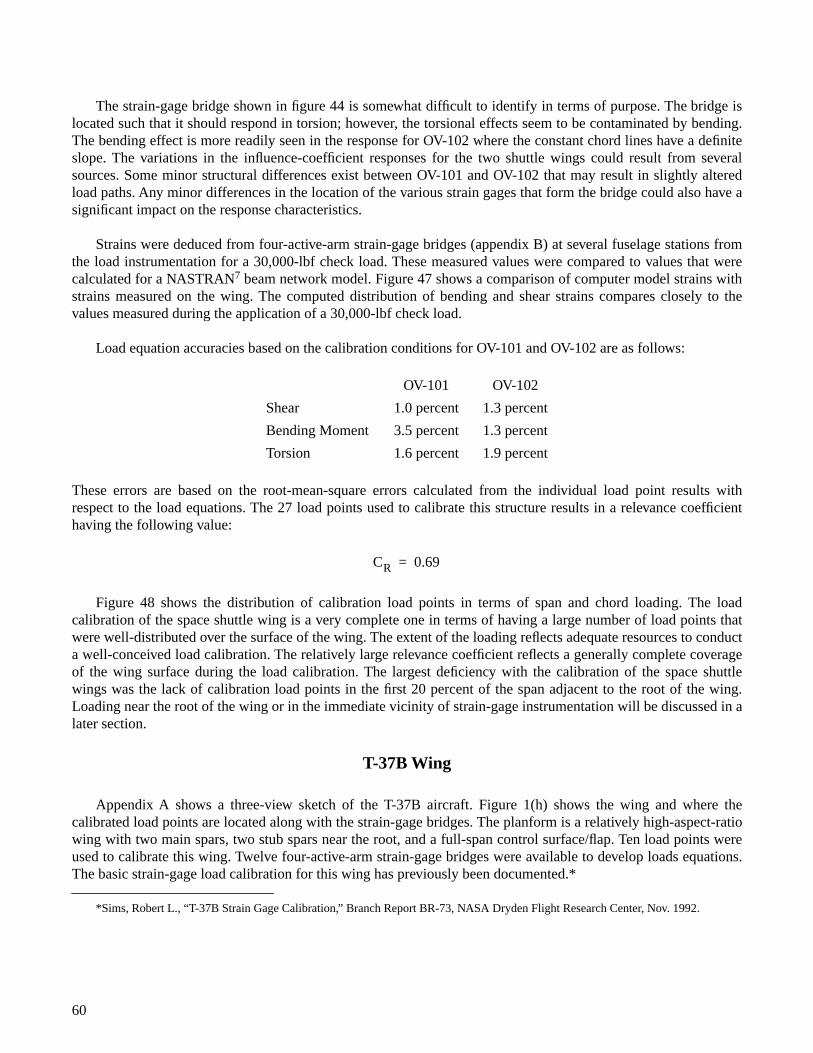
60
The strain-gage bridge shown in figure 44 is somewhat difficult to identify in terms of purpose. The bridge islocated such that it should respond in torsion; however, the torsional effects seem to be contaminated by bending.The bending effect is more readily seen in the response for OV-102 where the constant chord lines have a definiteslope. The variations in the influence-coefficient responses for the two shuttle wings could result from severalsources. Some minor structural differences exist between OV-101 and OV-102 that may result in slightly alteredload paths. Any minor differences in the location of the various strain gages that form the bridge could also have asignificant impact on the response characteristics.
Strains were deduced from four-active-arm strain-gage bridges (appendix B) at several fuselage stations fromthe load instrumentation for a 30,000-lbf check load. These measured values were compared to values that werecalculated for a NASTRAN7 beam network model. Figure 47 shows a comparison of computer model strains withstrains measured on the wing. The computed distribution of bending and shear strains compares closely to thevalues measured during the application of a 30,000-lbf check load.
Load equation accuracies based on the calibration conditions for OV-101 and OV-102 are as follows:
These errors are based on the root-mean-square errors calculated from the individual load point results withrespect to the load equations. The 27 load points used to calibrate this structure results in a relevance coefficienthaving the following value:
Figure 48 shows the distribution of calibration load points in terms of span and chord loading. The loadcalibration of the space shuttle wing is a very complete one in terms of having a large number of load points thatwere well-distributed over the surface of the wing. The extent of the loading reflects adequate resources to conducta well-conceived load calibration. The relatively large relevance coefficient reflects a generally complete coverageof the wing surface during the load calibration. The largest deficiency with the calibration of the space shuttlewings was the lack of calibration load points in the first 20 percent of the span adjacent to the root of the wing.Loading near the root of the wing or in the immediate vicinity of strain-gage instrumentation will be discussed in alater section.
T-37B Wing
Appendix A shows a three-view sketch of the T-37B aircraft. Figure 1(h) shows the wing and where thecalibrated load points are located along with the strain-gage bridges. The planform is a relatively high-aspect-ratiowing with two main spars, two stub spars near the root, and a full-span control surface/flap. Ten load points wereused to calibrate this wing. Twelve four-active-arm strain-gage bridges were available to develop loads equations.The basic strain-gage load calibration for this wing has previously been documented.*
*Sims, Robert L., “T-37B Strain Gage Calibration,” Branch Report BR-73, NASA Dryden Flight Research Center, Nov. 1992.
OV-101 OV-102
Shear 1.0 percent 1.3 percent
Bending Moment 3.5 percent 1.3 percent
Torsion 1.6 percent 1.9 percent
CR 0.69=
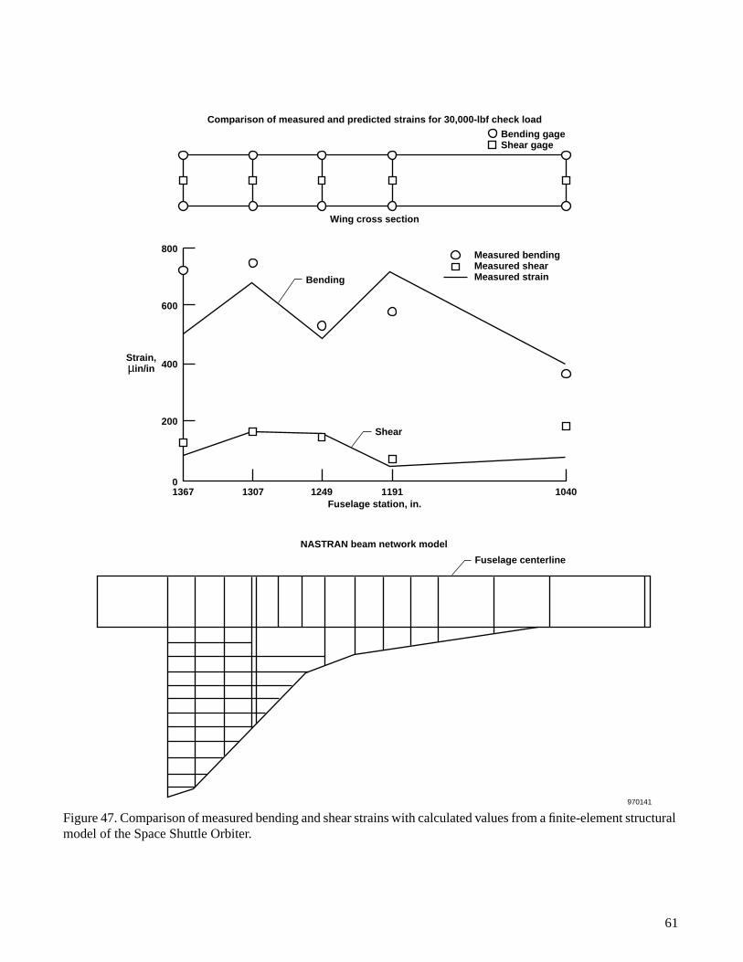
61
800
600
400
200
01307 1249
Strain,µin/in
1191
Shear
Bending
Measured bendingMeasured shearMeasured strain
Bending gageShear gage
1040Fuselage station, in.
NASTRAN beam network model
Wing cross section
Comparison of measured and predicted strains for 30,000-lbf check load
1367
Fuselage centerline
970141
Figure 47. Comparison of measured bending and shear strains with calculated values from a finite-element structuralmodel of the Space Shuttle Orbiter.
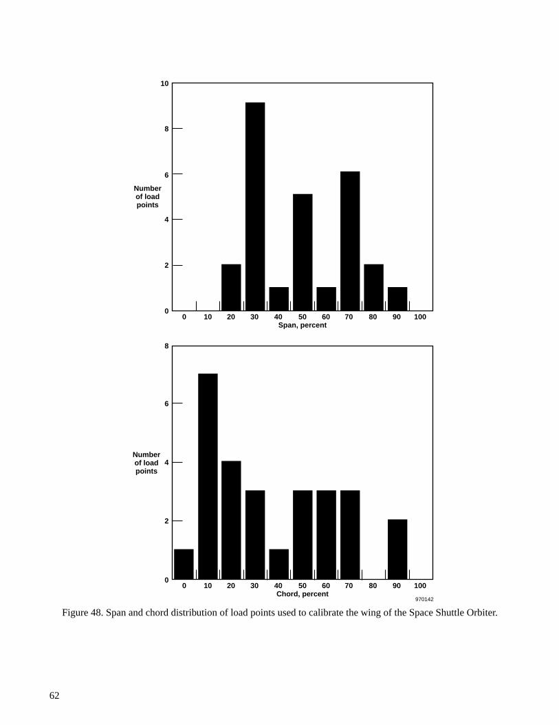
62
0 10 20 30 40 50Span, percent
60 70 80 90 100
0 10 20 30 40 50Chord, percent
60 70 80 90 100
970142
8
6
4Numberof loadpoints
2
10
8
6
4
Numberof loadpoints
2
0
0
Figure 48. Span and chord distribution of load points used to calibrate the wing of the Space Shuttle Orbiter.
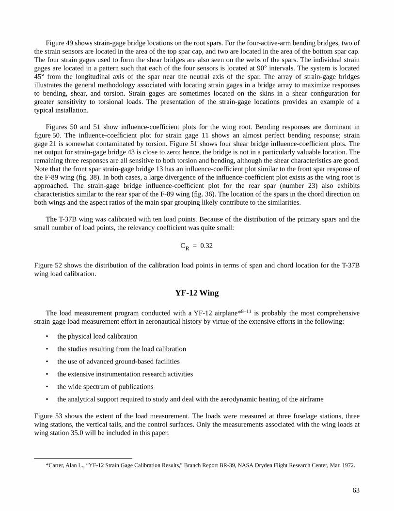
Figure 49 shows strain-gage bridge locations on the root spars. For the four-active-arm bending bridges, two ofthe strain sensors are located in the area of the top spar cap, and two are located in the area of the bottom spar cap.The four strain gages used to form the shear bridges are also seen on the webs of the spars. The individual straingages are located in a pattern such that each of the four sensors is located at 90° intervals. The system is located45° from the longitudinal axis of the spar near the neutral axis of the spar. The array of strain-gage bridgesillustrates the general methodology associated with locating strain gages in a bridge array to maximize responsesto bending, shear, and torsion. Strain gages are sometimes located on the skins in a shear configuration forgreater sensitivity to torsional loads. The presentation of the strain-gage locations provides an example of atypical installation.
Figures 50 and 51 show influence-coefficient plots for the wing root. Bending responses are dominant infigure 50. The influence-coefficient plot for strain gage 11 shows an almost perfect bending response; straingage 21 is somewhat contaminated by torsion. Figure 51 shows four shear bridge influence-coefficient plots. Thenet output for strain-gage bridge 43 is close to zero; hence, the bridge is not in a particularly valuable location. Theremaining three responses are all sensitive to both torsion and bending, although the shear characteristics are good.Note that the front spar strain-gage bridge 13 has an influence-coefficient plot similar to the front spar response ofthe F-89 wing (fig. 38). In both cases, a large divergence of the influence-coefficient plot exists as the wing root isapproached. The strain-gage bridge influence-coefficient plot for the rear spar (number 23) also exhibitscharacteristics similar to the rear spar of the F-89 wing (fig. 36). The location of the spars in the chord direction onboth wings and the aspect ratios of the main spar grouping likely contribute to the similarities.
The T-37B wing was calibrated with ten load points. Because of the distribution of the primary spars and thesmall number of load points, the relevancy coefficient was quite small:
Figure 52 shows the distribution of the calibration load points in terms of span and chord location for the T-37Bwing load calibration.
YF-12 Wing
The load measurement program conducted with a YF-12 airplane*8–11 is probably the most comprehensivestrain-gage load measurement effort in aeronautical history by virtue of the extensive efforts in the following:
• the physical load calibration
• the studies resulting from the load calibration
• the use of advanced ground-based facilities
• the extensive instrumentation research activities
• the wide spectrum of publications
• the analytical support required to study and deal with the aerodynamic heating of the airframe
Figure 53 shows the extent of the load measurement. The loads were measured at three fuselage stations, threewing stations, the vertical tails, and the control surfaces. Only the measurements associated with the wing loads atwing station 35.0 will be included in this paper.
*Carter, Alan L., “YF-12 Strain Gage Calibration Results,” Branch Report BR-39, NASA Dryden Flight Research Center, Mar. 1972.
CR 0.32=
63
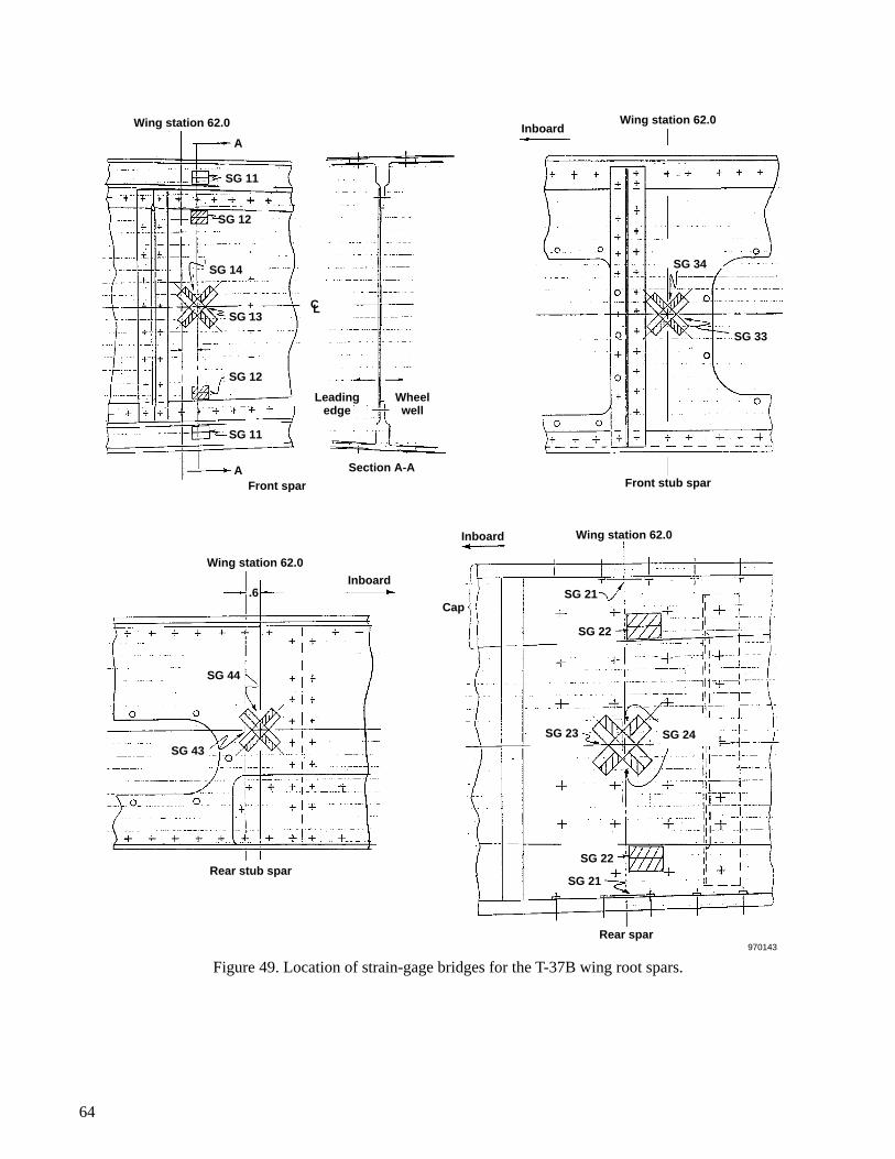
Rear stub spar
Rear spar970143
Inboard
Inboard
Cap.6
SG 44
SG 43SG 24
SG 21
SG 22
SG 23
SG 22
SG 21
Wing station 62.0
CL
A
A Section A-A
SG 11
SG 12
SG 14
SG 13
SG 12
SG 11
Wing station 62.0
Wing station 62.0
Wheelwell
Leadingedge
Front stub sparFront spar
SG 34
SG 33
InboardWing station 62.0
Figure 49. Location of strain-gage bridges for the T-37B wing root spars.
64

.200
.0001
.0002
.0003
.0004
.0005
.0006
.0007
.4
2040
6080
.6Span fraction
.8 1.0
970144
.2 .4 .6Span fraction
Strain gage 21 Strain gage 11Chord,percent
20
40
60
80
Chord, percent
LocationCalibration load points
Strain gages
11
Infl
uen
ce c
oef
fici
ent,
ou
tpu
t/lo
ad
.8 1.0
21
Figure 50. Influence-coefficient plots for typical bending strain-gage bridges for the T-37B wings.
65
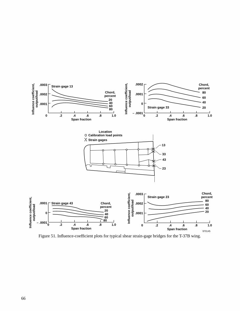
66
.2
.0001
.0001
– .0001
0
.0002
.0003
.4
204060
80
.6Span fraction
.8 1.0
.20 .4 .6Span fraction
.8 1.0.20 .4 .6Span fraction
.8 1.0
.20 .4 .6Span fraction
.8 1.0
970145
Strain gage 43
Strain gage 13
Strain gage 33
Strain gage 23
Chord,percent
20406080
Chord,percent
80
60
40
20
Chord,percent
80604020
Chord,percent
LocationCalibration load points
Strain gages
13
Infl
uen
ce c
oef
fici
ent,
ou
tpu
t/lo
adIn
flu
ence
co
effi
cien
t,o
utp
ut/
load
.0001
– .0001
0
.0001
.0002
.0002
.0003
0
Infl
uen
ce c
oef
fici
ent,
ou
tpu
t/lo
ad
Infl
uen
ce c
oef
fici
ent,
ou
tpu
t/lo
ad
33
43
23
Figure 51. Influence-coefficient plots for typical shear strain-gage bridges for the T-37B wing.

67
0 10 20 30 40 50Span, percent
60 70 80 90 100
0 10 20 30 40 50Chord, percent
60 70 80 90 100
970146
4
5
4
3
2
Numberof loadpoints
1
3
2
Numberof loadpoints
1
0
0
Figure 52. Distribution of load points in the span and chord directions for the T-37B wing load calibration.
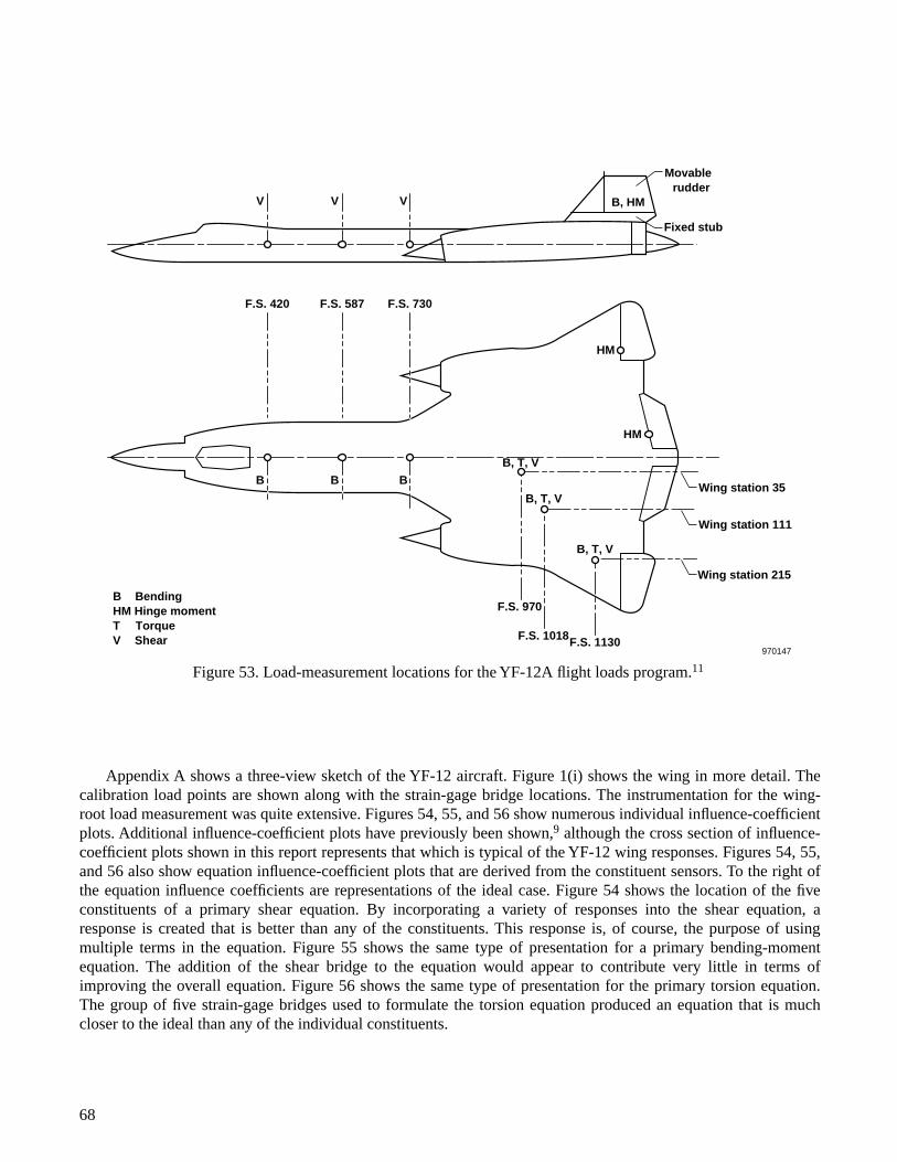
F.S. 1130
Wing station 215
Wing station 35
Wing station 111
B, T, V
B, T, V
BBB
B, T, V
HM
B, HM
Movable rudder
Fixed stub
HM
F.S. 1018
VVV
F.S. 730F.S. 587F.S. 420
B BendingHM Hinge momentT TorqueV Shear
F.S. 970
970147
Figure 53. Load-measurement locations for the YF-12A flight loads program.11
Appendix A shows a three-view sketch of the YF-12 aircraft. Figure 1(i) shows the wing in more detail. Thecalibration load points are shown along with the strain-gage bridge locations. The instrumentation for the wing-root load measurement was quite extensive. Figures 54, 55, and 56 show numerous individual influence-coefficientplots. Additional influence-coefficient plots have previously been shown,9 although the cross section of influence-coefficient plots shown in this report represents that which is typical of the YF-12 wing responses. Figures 54, 55,and 56 also show equation influence-coefficient plots that are derived from the constituent sensors. To the right ofthe equation influence coefficients are representations of the ideal case. Figure 54 shows the location of the fiveconstituents of a primary shear equation. By incorporating a variety of responses into the shear equation, aresponse is created that is better than any of the constituents. This response is, of course, the purpose of usingmultiple terms in the equation. Figure 55 shows the same type of presentation for a primary bending-momentequation. The addition of the shear bridge to the equation would appear to contribute very little in terms ofimproving the overall equation. Figure 56 shows the same type of presentation for the primary torsion equation.The group of five strain-gage bridges used to formulate the torsion equation produced an equation that is muchcloser to the ideal than any of the individual constituents.
68
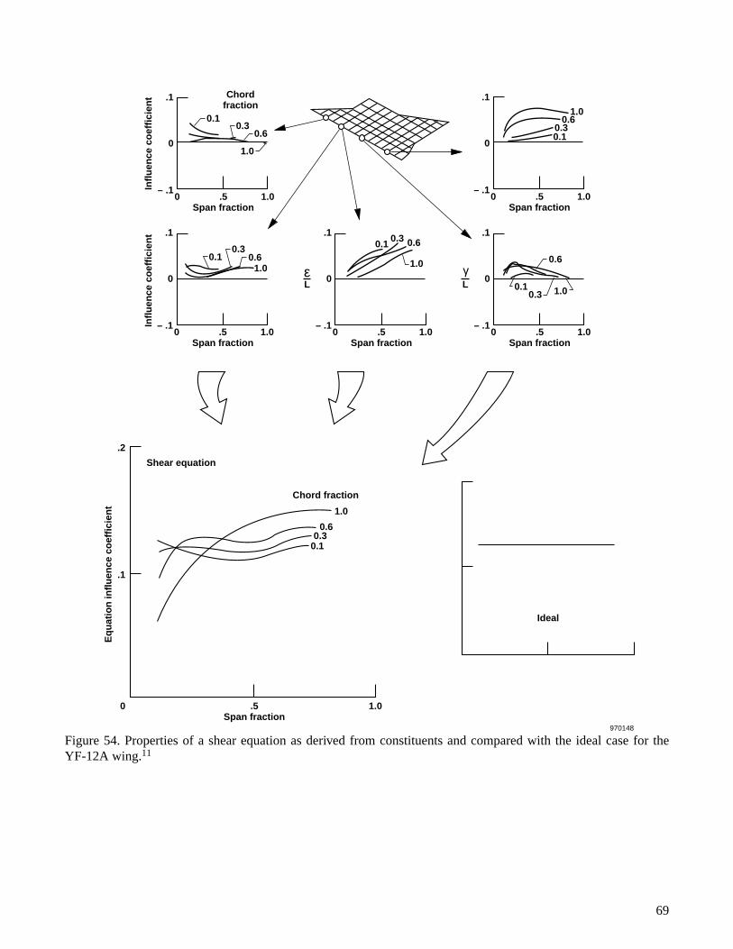
69
.5Span fraction
1.00
γL
– .1
0
.1
.5Span fraction
1.00
.5Span fraction
1.0
1.0
0.60.3
0.1
Chord fraction
Shear equation
Ideal
0
.1
.2
εL
– .1
0
.1
.5Span fraction
1.00
Infl
uen
ce c
oef
fici
ent
Eq
uat
ion
infl
uen
ce c
oef
fici
ent
Infl
uen
ce c
oef
fici
ent
– .1
0
.1
.5Span fraction
Chordfraction
1.0
1.0
0– .1
0
.1
0.10.3
0.6
1.00.1
0.30.6
1.0
0.1 0.3 0.6
1.00.10.3
0.6
1.0
0.10.3
0.6
.5Span fraction
1.00– .1
0
.1
970148
Figure 54. Properties of a shear equation as derived from constituents and compared with the ideal case for theYF-12A wing.11
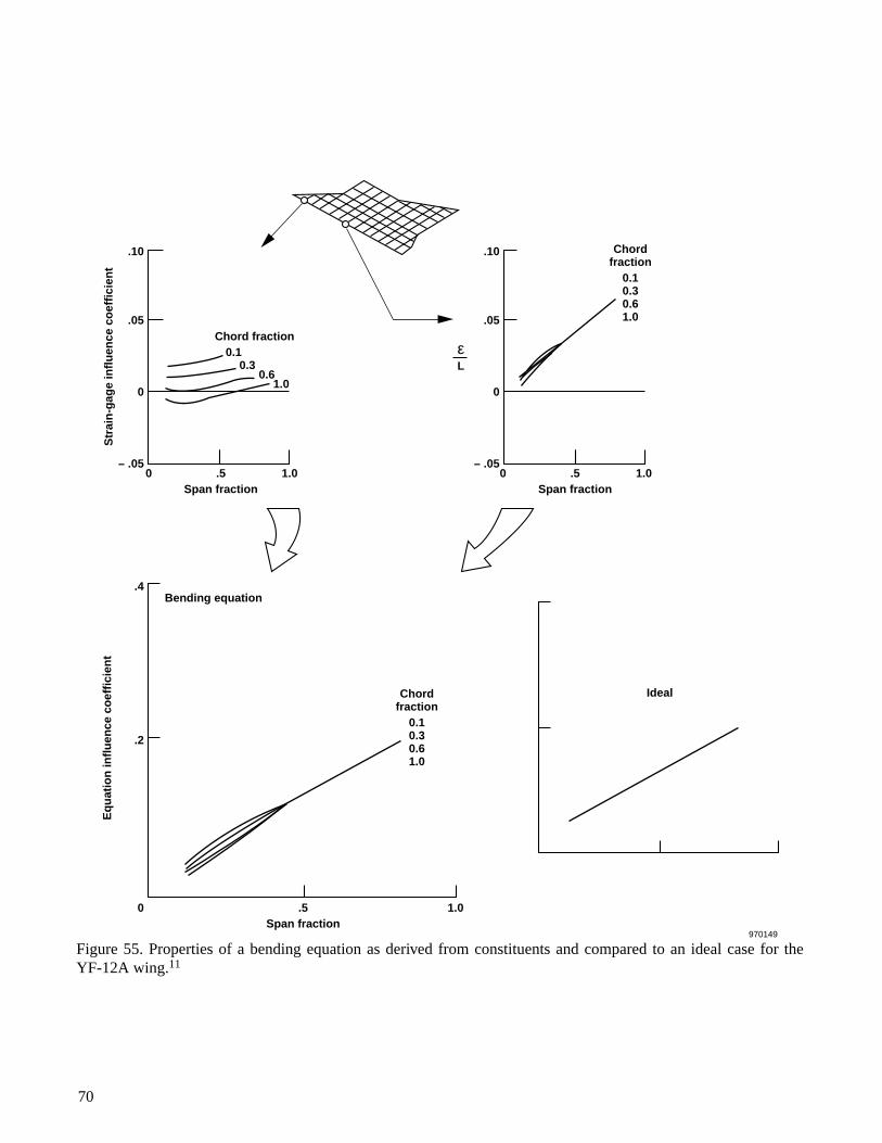
70
970149
Chordfraction
0.10.30.61.0
Chordfraction
0.10.30.61.0
.5Span fraction
1.00
0
– .05
.05
.10
Chord fraction
Str
ain
-gag
e in
flu
ence
co
effi
cien
t
.5Span fraction
1.00
.5Span fraction
1.0
Ideal
0
– .05
Eq
uat
ion
infl
uen
ce c
oef
fici
ent
.4Bending equation
.2
0
.05
.10
εL
1.00.6
0.30.1
Figure 55. Properties of a bending equation as derived from constituents and compared to an ideal case for theYF-12A wing.11
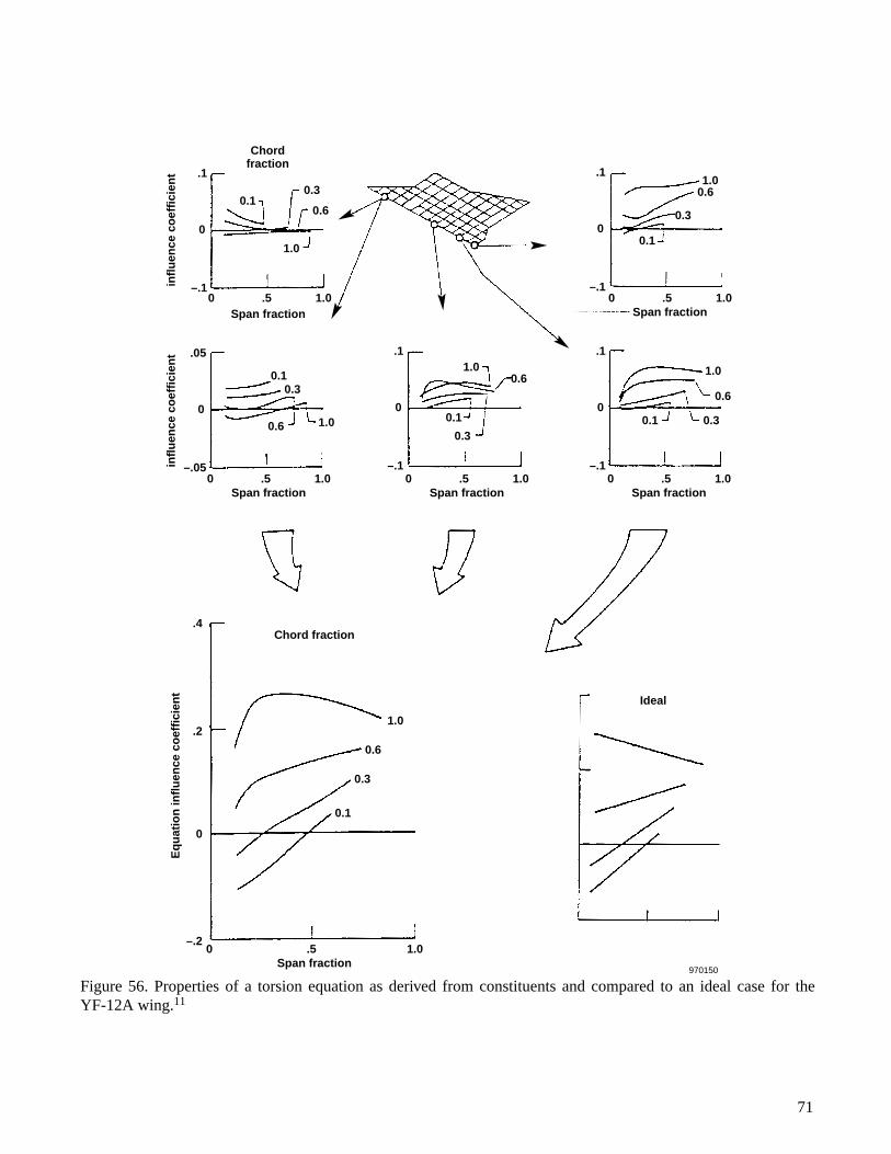
71
0
0
–.1
.1
.2
.4
–.2
970150Span fraction
Chord fraction
Chordfraction
Ideal
Eq
uat
ion
infl
uen
ce c
oef
fici
ent
0
–.1
.1
0
–.05
.05
infl
uen
ce c
oef
fici
ent
infl
uen
ce c
oef
fici
ent
.5 1.0
1.0
0.6
0.6
0.6
0.6
0.6
0.6
0.3
0.3
0.3
0.30.3
0.3
0.1
0.1
0.1 0.1
0.1
0
Span fraction.5 1.0
1.0
0
.5 1.00Span fraction
.5 1.00
Span fraction.5 1.00
Span fraction.5 1.00
0.11.0
1.0
1.0
1.0
0
–.1
.1
0
–.1
.1
Span fraction
Figure 56. Properties of a torsion equation as derived from constituents and compared to an ideal case for theYF-12A wing.11

One of the primary reasons that the YF-12 loads program was so valuable is that finite-element models of thestructure were developed to research the science of load measurement with strain gages. The simplified model (seeappendix C) of the wing (fig. 57) is of particular interest because of the insight that can be gained from a relativelyinexpensive and simple model. The individual calibration loads typically shown at the bottom right of figure 57were applied to both the model and the airplane in a laboratory; therefore, both measured and calculated influence-coefficient plots are available for comparison. Direct strains can also be compared (figs. 58 and 59). Shear strains(fig. 58) from the model are compared to shear strains measured for the same single-point loading conditions in thelaboratory. Figure 59 shows similar comparisons for bending strain. The overall comparison indicates promise interms of being able to predict strain from computer models. The strain gages on the YF-12 wing were wired infour-active-arm bridges, and the methodology used to convert this information to discrete strains is given inappendix B.
Figures 60 and 61 show a comparison of measured and calculated influence-coefficient plots for several strain-gage bridges located at several points along the root of the wing. Considering the simplicity of the model, thecomparison of calculated with measured influence-coefficient plots is amazingly good. This good comparison isattributed to the care with which the structural mechanics were input to formulate the elements of the NASTRANmodel. The careful detail of the modeling is considered to be so important that appendix D has been included toexplain how the structure was idealized. The comparison shown in figures 60 and 61 illustrates that the finite-element model can be effectively used to predict the nature of influence-coefficient plots for applied load points.The calculated values at the top right of figure 61 were somewhat larger than the measured values at the top left.
72
970151
NASTRAN bar model
Loading schematic asapplied to the model
Overhead restraining system forces
Nose gear reaction
Main landing gear reaction
Calibration load
Figure 57. YF-12A structural skeleton with the model representation and a typical load calibration condition.
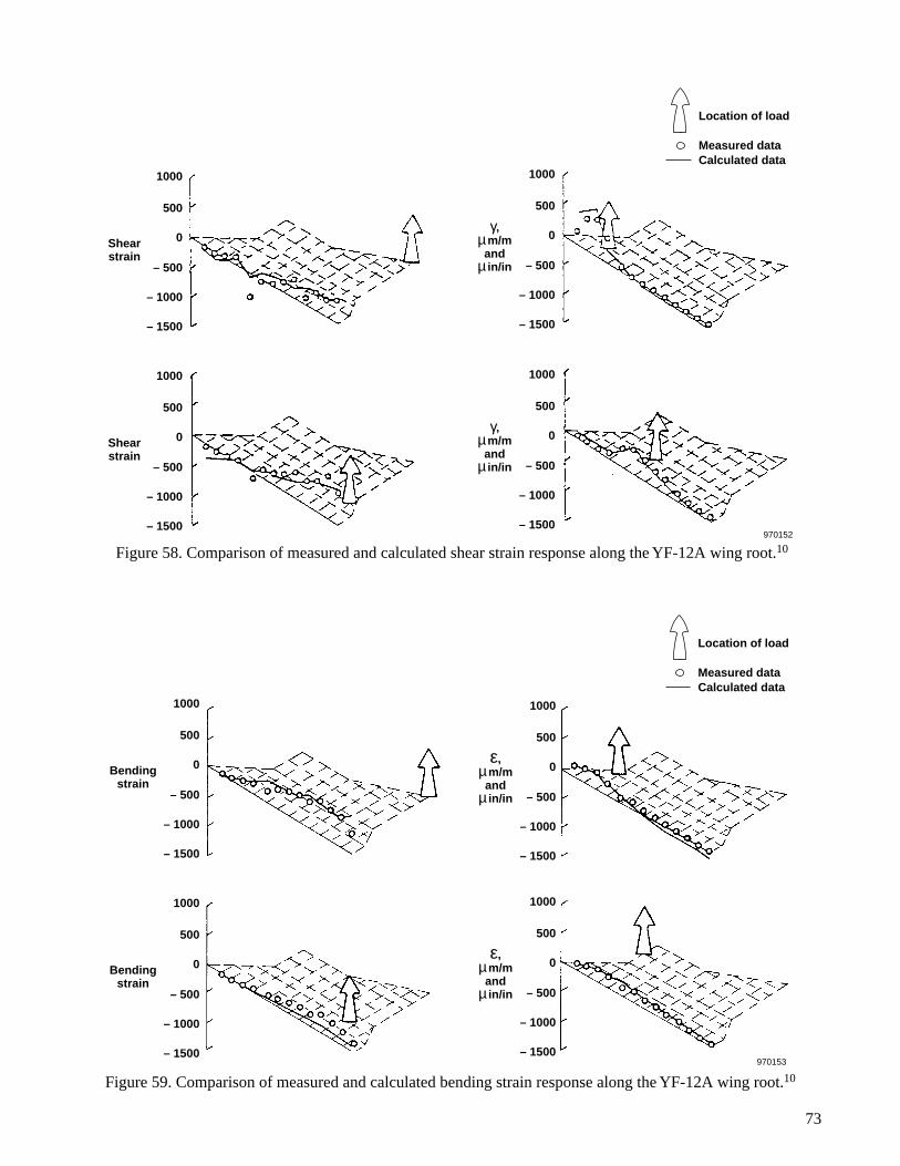
73
1000
500
0
– 500
– 1000
– 1500
1000
500
0
– 500
– 1000
– 1500
Shear strain
γ, µm/m
and µ in/in
1000
500
0
– 500
– 1000
– 1500
γ, µm/m
and µ in/in
1000
500
0
– 500
– 1000
– 1500
Shear strain
970152
Location of load Measured data Calculated data
Figure 58. Comparison of measured and calculated shear strain response along the YF-12A wing root.10
1000
500
0
– 500
– 1000
– 1500
1000
500
0
– 500
– 1000
– 1500
Bending strain
ε, µm/m
and µ in/in
1000
500
0
– 500
– 1000
– 1500
ε, µm/m
and µ in/in
1000
500
0
– 500
– 1000
– 1500
Bending strain
970153
Location of load Measured data Calculated data
Figure 59. Comparison of measured and calculated bending strain response along the YF-12A wing root.10
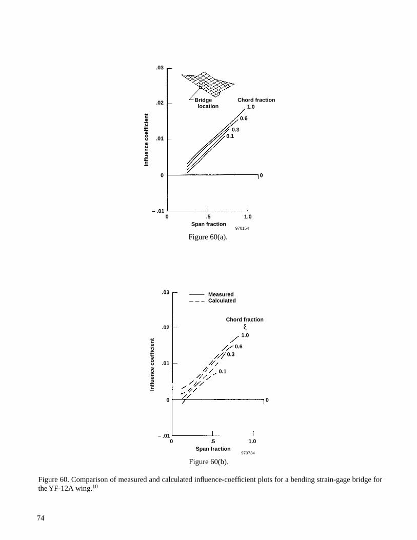
74
0 .5Span fraction
1.0
1.0
0.6
0.30.1
Chord fractionBridge location
0 0
.01
.02
.03
– .01
Infl
uen
ce c
oef
fici
ent
970154
Figure 60(a).
0 .5Span fraction
1.0
1.0
0.60.3
0.1
Chord fraction
MeasuredCalculated
0 0
.01
.02
.03
– .01
Infl
uen
ce c
oef
fici
ent
970734
ξ
Figure 60. Comparison of measured and calculated influence-coefficient plots for a bending strain-gage bridge forthe YF-12A wing.10
Figure 60(b).

75
.03
.02
.01
.01
0
–.02
–.01
.1
0
–.1
γ /L, µm/m
Nγ /L,
µ in/in
lbf
Bridge location
.03
.02
0
–.02
–.01
.1
0
–.1
γ /L, µm/m
N
γ /L, µ in/in
lbf
Bridge location
.01
.03
.02
0
–.02
–.01
.1
0
–.1
γ /L, µm/m
Nγ /L,
µ in/in
lbf
Bridge location
0.3
0.3
0.3
0.1
0.1
0.1
0.6
0.6
0.6
1.0
1.0
1.0
Measured Calculated
ξ
ξ
ξ
.03
.02
.01
.01
0
–.02
–.01
.1
0
–.1
γ /L, µm/m
Nγ /L,
µ in/in
lbf
.03
.02
0
–.02
–.01
.1
0
–.1
γ /L, µm/m
N
γ /L, µ in/in
lbf
.01
.03
.02
0
–.02
–.01
.1
0
–.1
γ /L, µm/m
N
γ /L, µ in/in
lbf
0.3
0.3
0.3
0.1
0.1
0.1
0η.5 1.0 0
η.5 1.0
0.6
0.6
0.6
1.0
1.0
1.0
ξ
ξ
ξ
970155
Figure 61. Comparison of measured and calculated influence-coefficient plots for shear strain-gage bridges on theYF-12A wing.10

The YF-12 wing was calibrated using 33 load points. Because the calibration was very extensive, the relevancycoefficient is a relatively large number:
Figure 62 shows the distribution of calibration load jacks. Any apparent discrepancy in the number of loadpoints is caused by the fact that some of the loading conditions involved two jacks applying the load in closeproximity. The aggregate of the two jacks can be considered a single load point for some purposes (such as thederivation of equations and influence-coefficient plots) but can be considered two loadings for other purposes(such as summarizing the extent of the surface load distributions).
Highly Maneuverable Aircraft Technology Wing
Appendix A shows a plan view of the Highly Maneuverable Aircraft Technology (HiMAT) aircraft. Figure 1(j)shows the HiMAT wing in more detail and where the calibrated load points are located along with the strain-gagebridges. The wing is of a moderate aspect ratio with two main spars. Seventeen load points were used to calibratethe strain-gage bridges on the HiMAT wing. This wing is unique in that the skin is a composite with reinforcinglayups tailored to the purpose of the wing. The sketch on the left side of figure 63 shows the principal direction ofthe ply lay-ups. When anisotropy is introduced to a wing, conventional influence-coefficient plots normally used toaid in bridge selection may not be valid. The validity depends on the degree and nature of the anisotropy. AppendixE gives a presentation of the physics of anisotropy with regard to the interpretation of influence coefficients withrespect to strain-gage load calibrations.
The anisotropy associated with the skin does not appear to be significant enough to have a major effect on thetraditional appearance of the influence-coefficient plot for the bending-moment bridge, B2. The plot shows abending response that is characteristically the same as for other bending-moment plots (fig. 63). The onlydistinguishing difference is a larger-than-usual torsional spread. No clear reason exists to believe that this torsionalspread is caused by the anisotropy.
The influence-coefficient plots shown in figure 64 exhibit characteristics that could be affected by theanisotropic skins. In the traditional sense, the plots do not appear to be favorable, particularly for sensing shear.The overall outputs are very low. Strain-gage bridges S1 and S2 both change sign in the span direction. This effectcould be interpreted as not a traditionally favorable response. The basic difference between elasticityand anisotropic elasticity is addressed in some detail in appendix E, where the basic anisotropic equationsare presented.
The 17 load points used to calibrate the HiMAT wing resulted in the following relevancy coefficient:
Figure 65 shows the distribution of the calibration load points in terms of span and chord. Additional informationregarding the HiMAT wing and the general program has previously been given.12–14
Supercritical Wing
Appendix A shows a three-view sketch of an F-8 aircraft modified to fly with a supercritical wing. Figure 1(k)shows where the calibration load points are located on the wing along with the strain-gage bridges. Thesupercritical wing is a high-aspect-ratio, high-degree-of-sweep wing with trailing-edge high-lift devices. Twenty-eight load points were used (fig. 66) to calibrate this wing panel. Figure 1(k) shows the general location of thestrain-gage bridges. The information relating to the supercritical wing load calibration has been developed fromunpublished, undocumented files and notebooks of Aerostructures Branch personnel at NASA Dryden. Someinformation regarding the program has been published.15, 16 The strain-gage bridges are located on or about thethree primary spars. This wing structure has the highest aspect ratio of any lifting surface included in this report.
CR 0.70=
CR 0.51=
76
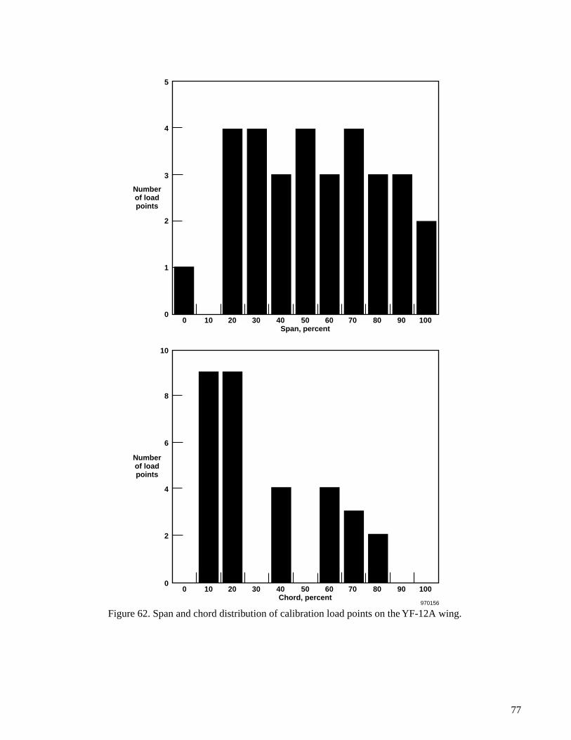
77
0 10 20 30 40 50Span, percent
60 70 80 90 100
0 10 20 30 40 50Chord, percent
60 70 80 90 100
970156
10
8
6
Numberof loadpoints
4
2
5
4
3
2
Numberof loadpoints
1
0
0
Figure 62. Span and chord distribution of calibration load points on the YF-12A wing.

78
.1
.2
.3
.4
Span fraction.2
15
55
40
Chord,percent
HiMAT wing SG bridge B2
Infl
uen
ce c
oef
fici
ent,
ou
tpu
t/lo
ad
0
S1T1
B1B2
S2
– 50°
50°
35°0
.4 .6 .8 1.0
970157
–.05
0
.05
Span fraction
HiMAT wing SG bridge S1
.2
HiMAT wing SG bridge S2
80
55
55
55
30
30
30
15
15
15
Chord,percent
80
80
HiMAT wing SG bridge T1
Infl
uen
ce c
oef
fici
ent,
ou
tpu
t/lo
ad
–.05
0
.05
Infl
uen
ce c
oef
fici
ent,
ou
tpu
t/lo
ad
–.05
0
.05
Infl
uen
ce c
oef
fici
ent,
ou
tpu
t/lo
ad
0
S1
T1
B1
B2
S2
– 50°
50°
35°0
.4 .6 .8 1.0
970158
Chord,percent
Chord,percent
Figure 63. Influence-coefficient plot for a bending strain-gage bridge on the HiMAT aircraft wing.
Figure 64. Influence-coefficient plots for strain-gage bridges configured for sensing shear on the HiMATaircraft wing.
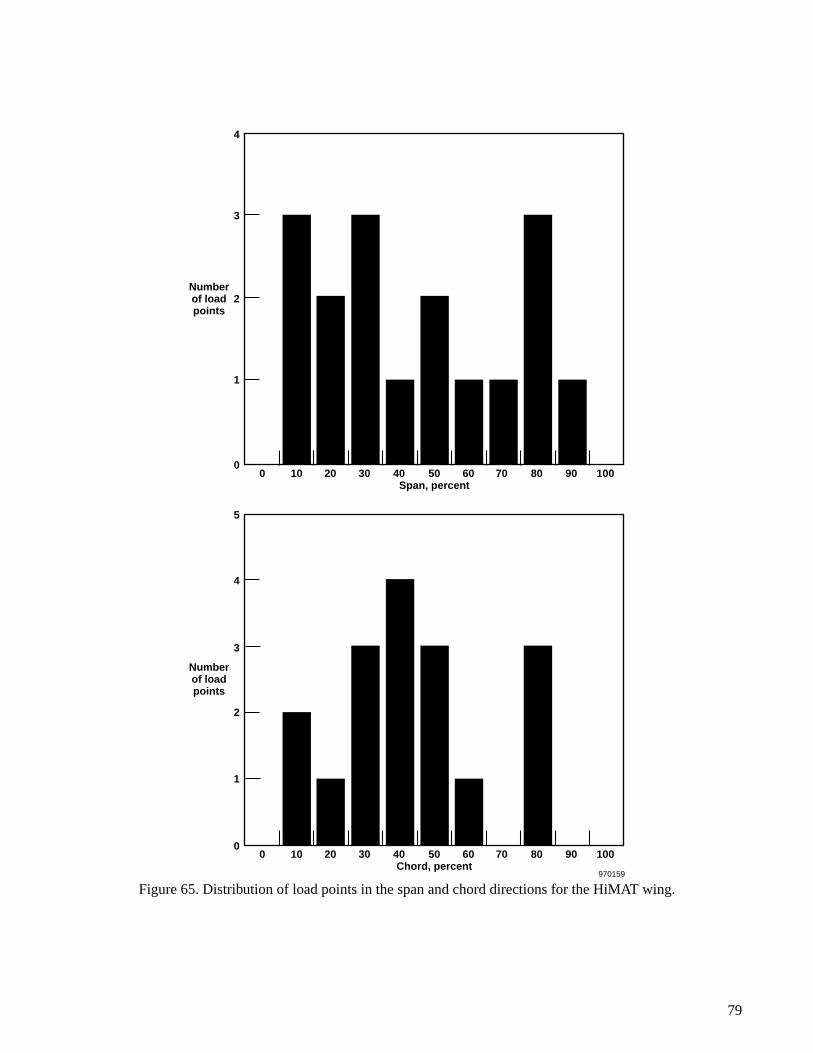
79
0 10 20 30 40 50Span, percent
60 70 80 90 100
0 10 20 30 40 50Chord, percent
60 70 80 90 100
970159
4
3
2Numberof loadpoints
1
5
4
3
2
Numberof loadpoints
1
0
0
Figure 65. Distribution of load points in the span and chord directions for the HiMAT wing.
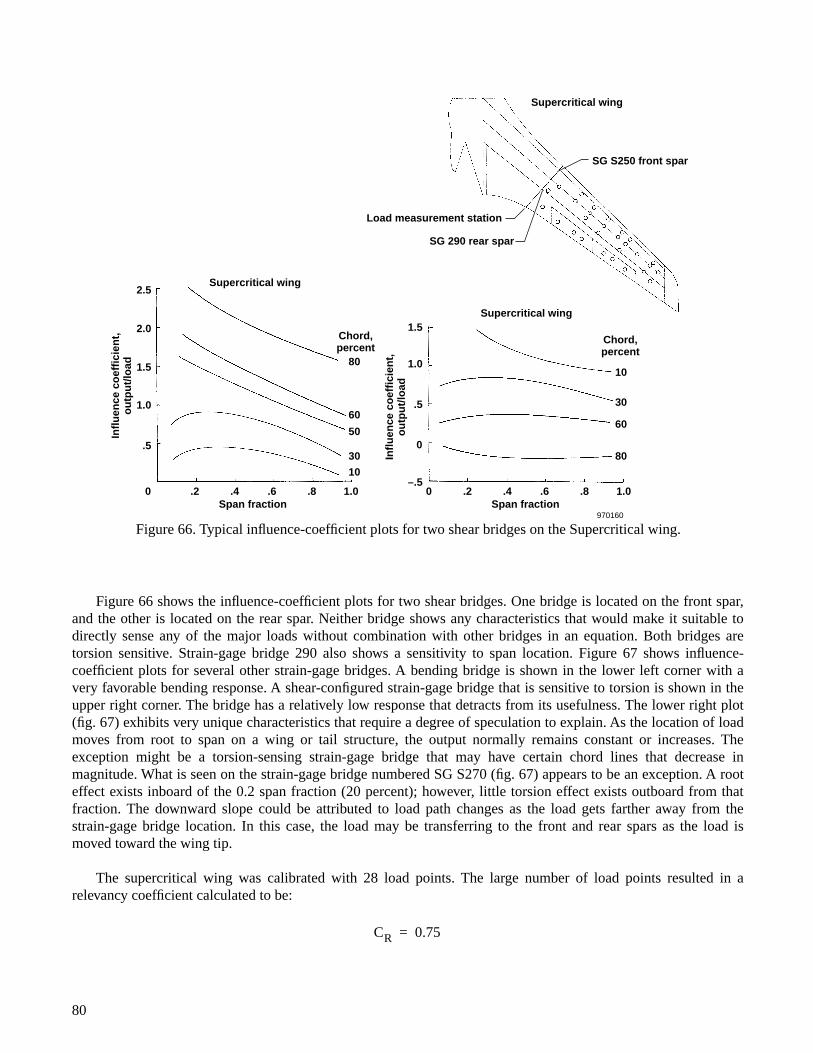
.5
.5
–.5
2.0
2.5
1.5
1.5
1.0
1.0
Span fraction.2 .4 .6 .8 1.0
Span fraction.20 .4 .6 .8 1.0
60
50
30
10
10
Load measurement station
SG 290 rear spar
SG S250 front spar
30
60
80
80
Chord, percent
Chord, percent
Supercritical wing
Supercritical wing
Supercritical wingIn
flu
ence
co
effi
cien
t,
ou
tpu
t/lo
ad
Infl
uen
ce c
oef
fici
ent,
o
utp
ut/
load
0
0
970160
Figure 66. Typical influence-coefficient plots for two shear bridges on the Supercritical wing.
Figure 66 shows the influence-coefficient plots for two shear bridges. One bridge is located on the front spar,and the other is located on the rear spar. Neither bridge shows any characteristics that would make it suitable todirectly sense any of the major loads without combination with other bridges in an equation. Both bridges aretorsion sensitive. Strain-gage bridge 290 also shows a sensitivity to span location. Figure 67 shows influence-coefficient plots for several other strain-gage bridges. A bending bridge is shown in the lower left corner with avery favorable bending response. A shear-configured strain-gage bridge that is sensitive to torsion is shown in theupper right corner. The bridge has a relatively low response that detracts from its usefulness. The lower right plot(fig. 67) exhibits very unique characteristics that require a degree of speculation to explain. As the location of loadmoves from root to span on a wing or tail structure, the output normally remains constant or increases. Theexception might be a torsion-sensing strain-gage bridge that may have certain chord lines that decrease inmagnitude. What is seen on the strain-gage bridge numbered SG S270 (fig. 67) appears to be an exception. A rooteffect exists inboard of the 0.2 span fraction (20 percent); however, little torsion effect exists outboard from thatfraction. The downward slope could be attributed to load path changes as the load gets farther away from thestrain-gage bridge location. In this case, the load may be transferring to the front and rear spars as the load ismoved toward the wing tip.
The supercritical wing was calibrated with 28 load points. The large number of load points resulted in arelevancy coefficient calculated to be:
CR 0.75=
80
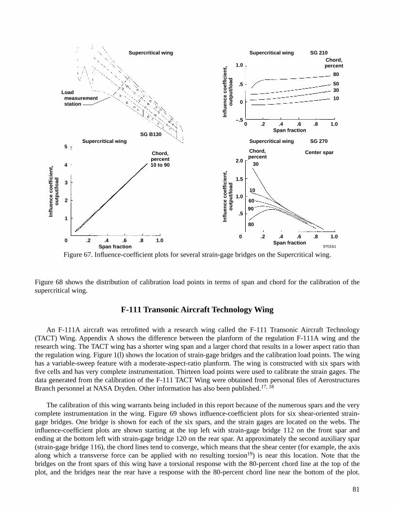
5
2.0
1.5
1.0
.5
4
3
2
1
Span fraction.4 .6 .8 1.0.20 Span fraction
.4 .6 .8 1.0.2
Span fraction.4 .6 .8 1.0.20
0
1.0
.5
–.5
0
Load measurement station
Chord, percent 10 to 90
Chord, percent
Chord, percent
30
80
5030
10
10
60
90
80
Supercritical wing
Supercritical wing
SG B130Supercritical wing SG 270
Center spar
Supercritical wing SG 210In
flu
ence
co
effi
cien
t,
ou
tpu
t/lo
ad
Infl
uen
ce c
oef
fici
ent,
o
utp
ut/
load
Infl
uen
ce c
oef
fici
ent,
o
utp
ut/
load
970161
Figure 67. Influence-coefficient plots for several strain-gage bridges on the Supercritical wing.
Figure 68 shows the distribution of calibration load points in terms of span and chord for the calibration of thesupercritical wing.
F-111 Transonic Aircraft Technology Wing
An F-111A aircraft was retrofitted with a research wing called the F-111 Transonic Aircraft Technology(TACT) Wing. Appendix A shows the difference between the planform of the regulation F-111A wing and theresearch wing. The TACT wing has a shorter wing span and a larger chord that results in a lower aspect ratio thanthe regulation wing. Figure 1(l) shows the location of strain-gage bridges and the calibration load points. The winghas a variable-sweep feature with a moderate-aspect-ratio planform. The wing is constructed with six spars withfive cells and has very complete instrumentation. Thirteen load points were used to calibrate the strain gages. Thedata generated from the calibration of the F-111 TACT Wing were obtained from personal files of AerostructuresBranch personnel at NASA Dryden. Other information has also been published.17, 18
The calibration of this wing warrants being included in this report because of the numerous spars and the verycomplete instrumentation in the wing. Figure 69 shows influence-coefficient plots for six shear-oriented strain-gage bridges. One bridge is shown for each of the six spars, and the strain gages are located on the webs. Theinfluence-coefficient plots are shown starting at the top left with strain-gage bridge 112 on the front spar andending at the bottom left with strain-gage bridge 120 on the rear spar. At approximately the second auxiliary spar(strain-gage bridge 116), the chord lines tend to converge, which means that the shear center (for example, the axisalong which a transverse force can be applied with no resulting torsion19) is near this location. Note that thebridges on the front spars of this wing have a torsional response with the 80-percent chord line at the top of theplot, and the bridges near the rear have a response with the 80-percent chord line near the bottom of the plot.
81
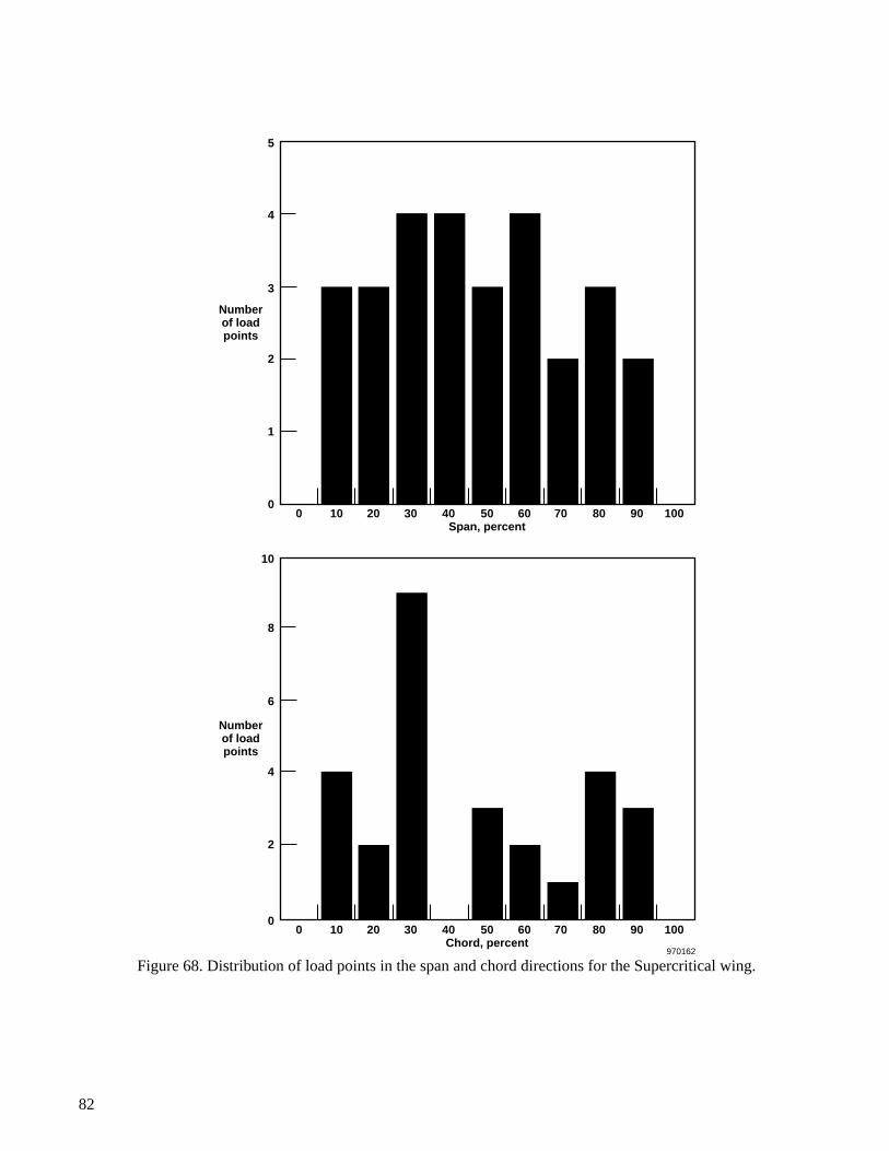
82
0 10 20 30 40 50Span, percent
60 70 80 90 100
0 10 20 30 40 50Chord, percent
60 70 80 90 100
970162
10
Numberof loadpoints
5
4
3
2
Numberof loadpoints
1
8
6
4
2
0
0
Figure 68. Distribution of load points in the span and chord directions for the Supercritical wing.
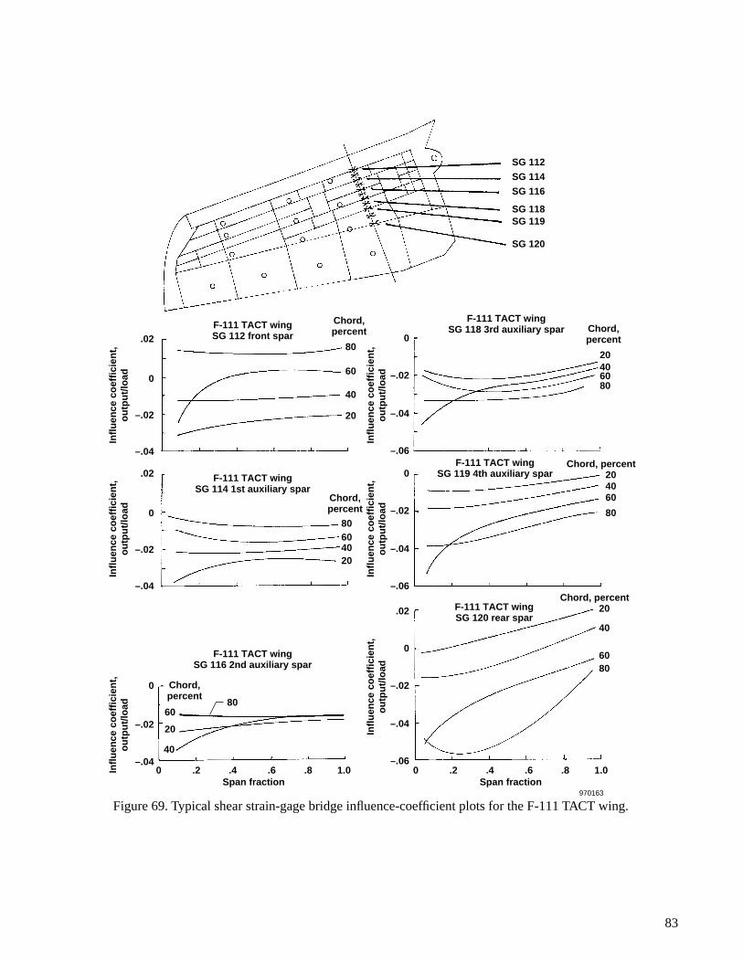
83
0
–.04
–.02
0
.02
–.02
–.04 –.06
–.04
–.02
0
–.06
–.04
–.02
0
.02
Span fraction
–.04
–.02
0
.02
Infl
uen
ce c
oef
fici
ent,
ou
tpu
t/lo
adIn
flu
ence
co
effi
cien
t,o
utp
ut/
load
Infl
uen
ce c
oef
fici
ent,
ou
tpu
t/lo
ad
Infl
uen
ce c
oef
fici
ent,
ou
tpu
t/lo
adIn
flu
ence
co
effi
cien
t,o
utp
ut/
load
Infl
uen
ce c
oef
fici
ent,
ou
tpu
t/lo
ad
–.06
–.04
–.02
0
.4.20 .6 .8 1.0Span fraction
.4.20 .6 .8 1.0
Chord,percent
F-111 TACT wingSG 114 1st auxiliary spar
F-111 TACT wingSG 116 2nd auxiliary spar
F-111 TACT wingSG 118 3rd auxiliary spar
F-111 TACT wingSG 119 4th auxiliary spar
F-111 TACT wingSG 120 rear spar
F-111 TACT wingSG 112 front spar
80
Chord,percent
Chord,percent
Chord,percent
20406080
80
Chord, percent20
Chord, percent20
40
6080
60
20
40
80
4060
80
604020
60
40
20
SG 112
SG 114
SG 116
SG 118SG 119
SG 120
970163
Figure 69. Typical shear strain-gage bridge influence-coefficient plots for the F-111 TACT wing.

It is obvious that if a strain-gage bridge with a pure shear response is sought, then a likely place to locate shearbridges is near the shear center. The influence-coefficient plot for strain-gage bridge 116 exemplifies a very goodshear bridge. Locating shear bridges on spars near the shear center is probably a good rule to use on moderate- andhigh-aspect-ratio lifting-surface structures. Low-aspect-ratio lifting-surface structures are less likely to exhibitsuch a trait.
Figure 70 shows the influence-coefficient plots for two bridges located on the skin between spars. Thesebridges are configured and located to sense torsional loads. These two influence-coefficient plots are presented toillustrate the response of strain-gage bridges located on the skin of the structures. The strain-gage bridge responsesfor the influence-coefficient plots shown in figure 71 are typically bending in nature. Strain-gage bridge 102 islocated on the spar caps near the shear center. The bridge appears to sense bending without contamination fromshear or torsion. The influence-coefficient plot for strain-gage bridge 106 shows the bridge to be somewhatcontaminated with torsion, particularly for the load points on the control surfaces. This strain-gage bridge islocated considerably aft of the shear center.
The F-111 TACT Wing was calibrated with 13 load points that resulted in a relevancy coefficient of:
Figure 72 shows the distribution of the calibration load points in terms of spar and chord location.
B-2 Wing
Most of the specific details of the calibration of the B-2 wing remain obscure because of classificationconsiderations. Enough information is available, however, to extract some valuable information relative to thescience of calibrated strain gages and to current characteristics of airplane load calibrations.
Appendix A shows a plan view of the B-2 aircraft. Figure 1(m) shows the B-2 wing in more detail and wherethe calibration load points are located along with the strain-gage bridges. The wing is extensively instrumentedwith strain gages. The structural arrangement is very complex, with spars and ribs intersecting obliquely. The loadpoints are not widely distributed over the surface of the wing. Further, the loads were not applied individually assuggested1 but were applied as a relatively small number of distributed loads with many individual jacks usedsimultaneously.
Figure 73 shows the distribution of jack points. A major portion of the wing obviously has no applied loads.Because of the nature of the outer surface of the wing, structure loads could only be applied to the forward and therear parts of the wing surface, which raises several questions about the philosophy of the load calibration. If amajor part of the surface of the wing cannot be loaded, then how can flight loads in that area be interpreted? Inaddition, a discrete load calibration was not conducted; a distributed load calibration was used instead. The basicphilosophy behind the two contrasting approaches (discrete rather than distributed) to calibrating has really notbeen discussed. The method of calibration (calibration methods will be addressed in the Discussion section) is notas important as the significance of the large unloaded area that would similarly affect either load calibrationapproach. The casual observer would question the validity of a load calibration that has such a large portion of theproblem missing.
Although the data cannot be presented in this report, the load calibration was considered to be satisfactorybecause the flight measurements correlated well with predicted loads. Figure 74 shows a possible explanation forthis correlation. A classic subsonic load distribution20 is shown at the top of the figure, and the distribution of theapplied calibration loads is shown at the bottom of the figure. The primary distribution of this flight loadis centered in the forward part of the chord of the wing. The application of calibration loads in the area where theflight loads are dominant provides an explanation of why the load calibration was thought to be valid.
CR 0.50=
84
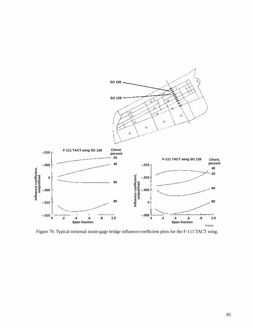
85
–.005
0
–.005
–.010
–.015
Span fraction.4.20 .6 .8 1.0
Span fraction.4.20 .6 .8 1.0
F-111 TACT wing SG 126 Chord,percent
20
40
60
80
F-111 TACT wing SG 128 Chord,percent
40
20
60
80
SG 126
SG 128
970164
Infl
uen
ce c
oef
fici
ent,
ou
tpu
t/lo
ad
–.015
–.010
–.005
0
–.005
–.010
Infl
uen
ce c
oef
fici
ent,
ou
tpu
t/lo
ad
Figure 70. Typical torsional strain-gage bridge influence-coefficient plots for the F-111 TACT wing.
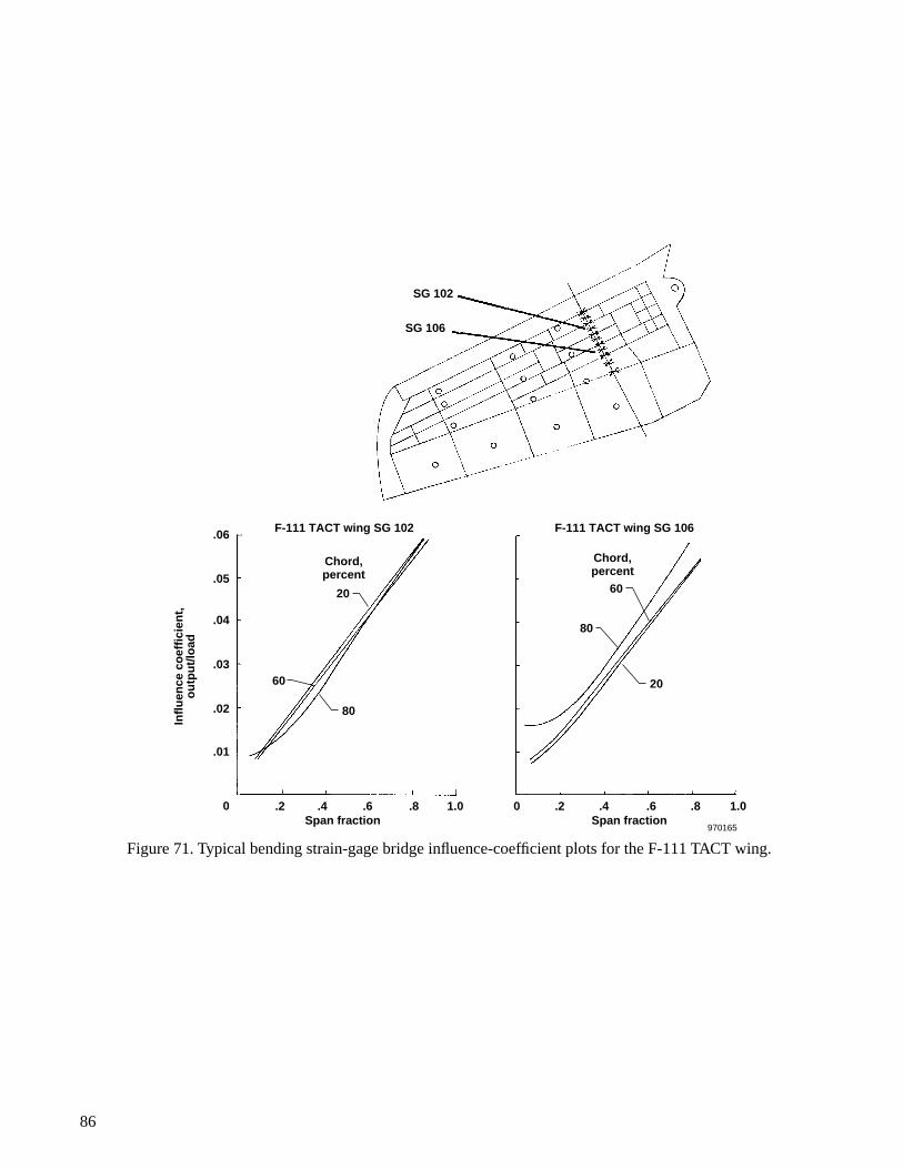
86
Span fraction.4.20 .6 .8 1.0
Span fraction.4.2 .6 .8 1.0
Chord,percent
20
60
80
SG 102
SG 106
970165
0
.01
.02
.03
.04
.05
.06
Infl
uen
ce c
oef
fici
ent,
ou
tpu
t/lo
ad
Chord,percent
60
80
20
F-111 TACT wing SG 102 F-111 TACT wing SG 106
Figure 71. Typical bending strain-gage bridge influence-coefficient plots for the F-111 TACT wing.
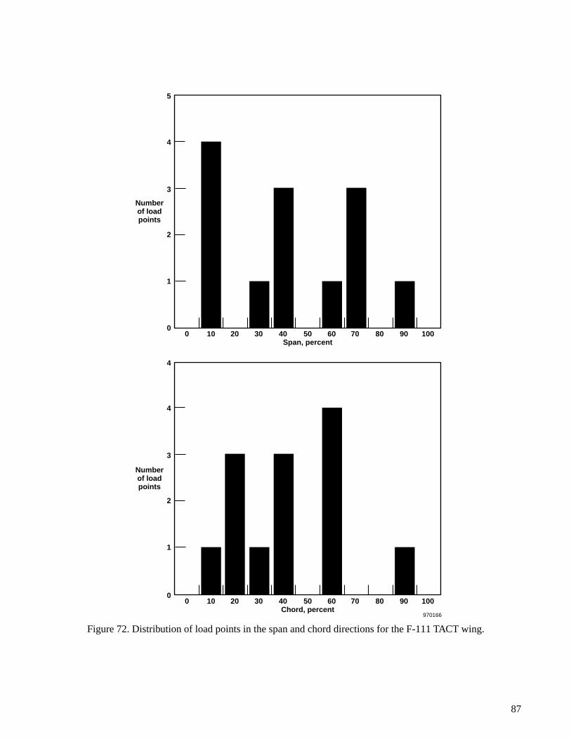
87
0 10 20 30 40 50Span, percent
60 70 80 90 100
0 10 20 30 40 50Chord, percent
60 70 80 90 100
970166
4
Numberof loadpoints
5
4
3
2
Numberof loadpoints
1
4
3
2
1
0
0
Figure 72. Distribution of load points in the span and chord directions for the F-111 TACT wing.

88
0 10 20 30 40 50Span, percent
60 70 80 90 100
0 10 20 30 40 50Chord, percent
60 70 80 90 100
970167
8
6
4Numberof loadpoints
2
20
10Numberof loadpoints
0
0
Figure 73. Span and chord distribution of load points on the B-2 wing.

89
Span direction Chord direction
Su
bso
nic
dis
trib
uti
on
Su
rfac
e lo
ad
Span direction Chord direction
Lo
ad c
alib
rati
on
dis
trib
uti
on
Su
rfac
e lo
ad
970168
Figure 74. Comparison of a subsonic load distribution with the load calibration loads on the B-2 wing.

A second typical wing load distribution should be considered in evaluating the validity of the basic loadcalibration. A totally different load distribution occurs when the control surfaces are deflected. This difference issomewhat more difficult to identify in a classic sense; however, the primary result is to add load to the rear of thestructure. Figure 74 shows that the spectrum of the load calibration also includes some large calibration loads inthe rear of the wing. The two primary load distributions are safely assumed to be covered by the spectrum of loadsused for the calibration. The two areas where flight load was concentrated largely corresponded to the two areaswhere large loads were applied during the load calibration.
The nature of the B-2 wing raises some very provocative thoughts relative to the strain-gage calibrations offuture aircraft. If, in the future, large surface areas of wings cannot be physically loaded, then pursuing alternateapproaches is logically prudent. Figure 75 shows two such approaches that are pertinent for both the B-2 wing andother aircraft. One approach involves using a finite-element structural model to develop a load calibrationanalytically. An incomplete loading such as the B-2 wing case could serve as a check load to verify the accuracy ofthe load equations developed from the analytical model. This idea is depicted in the right side of figure 75, wherethe square symbols represent analytical load points applied to the finite-element model from which load equationsare developed. The accuracy of the analytically established load equations would then be verified by some type ofphysical loading such as is depicted as a check load by the circular symbols.
A second approach is shown in the left side of figure 75, where a hybrid load calibration is suggested. The ideain this approach is to apply physical loads to the structure where possible and augment these loads with analyticalloadings using a finite-element structural model in the areas where load cannot be physically applied. Both of theapproaches shown in figure 75 require a level of confidence in the accuracy of an analytical structural model.Structural modeling will be addressed in the Discussion section.
Eleven distributed-load calibration conditions were used to calibrate the structure. The aggregate of all loadpoints resulted in a relevancy coefficient of:
Figure 73 shows the distribution of these loads.
B-1 Wing
The strain-gage loads calibration of the B-1 wing provides one of the more unique aspects of all structurespresented in this document. The strain-gage bridges were calibrated independently at different times using adistributed-load method in one case and a point-load method in another case. Equations were derived for bothapproaches using the same set of strain-gage bridges. This circumstance provides the opportunity to comparecalculated flight loads using equations that have been derived with different calibration methods.
The B-1 wing is a high-aspect-ratio variable-sweep lifting surface with a configuration typical of this family ofconfigurations that began with the F-111 airplane. Appendix A shows a three-view drawing of the B-1 aircraft.Figure 1(n) shows the B-1 wing in more detail and where the calibration load points and strain-gage bridges arelocated. The structural arrangement is relatively simple for a modern aircraft. Two primary spars (front and rear)exist from which leading- and trailing-edge control surfaces are cantilevered. The arrangements of the jack pointsfor the point-load calibration is very straightforward, with the load points being applied at six span stations alongthree constant chord lines. The 18 load points provide a well-balanced distribution of applied loads. Thedistributed-load calibration was developed from static test loads that correspond to wing design conditions.Information concerning the distributed-load calibration has previously been published.21 Information concerningthe point-load calibration has been given.*
*Schuster, Lawrence S., “B-1 Point Load Calibration,” Memorandum to Aerostructures Branch Files, NASA Dryden Flight ResearchCenter, July 1981.
CR 0.45=
90
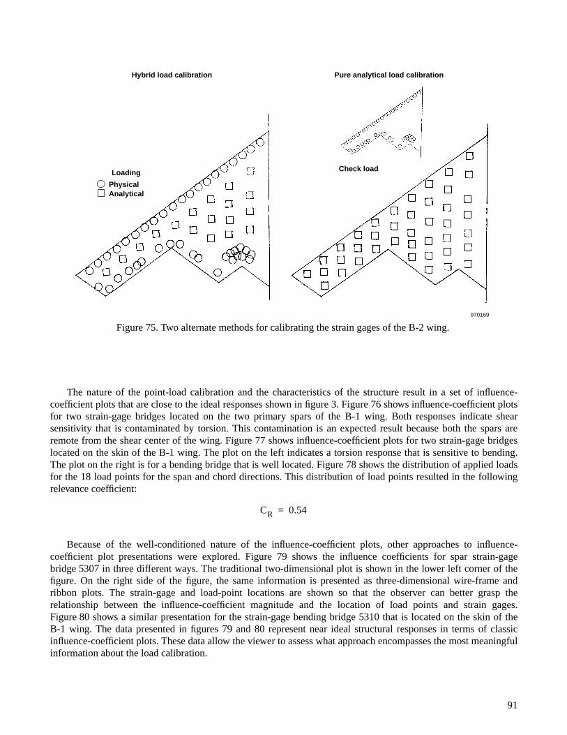
970169
Physical Analytical
Loading
Pure analytical load calibration
Check load
Hybrid load calibration
Figure 75. Two alternate methods for calibrating the strain gages of the B-2 wing.
The nature of the point-load calibration and the characteristics of the structure result in a set of influence-coefficient plots that are close to the ideal responses shown in figure 3. Figure 76 shows influence-coefficient plotsfor two strain-gage bridges located on the two primary spars of the B-1 wing. Both responses indicate shearsensitivity that is contaminated by torsion. This contamination is an expected result because both the spars areremote from the shear center of the wing. Figure 77 shows influence-coefficient plots for two strain-gage bridgeslocated on the skin of the B-1 wing. The plot on the left indicates a torsion response that is sensitive to bending.The plot on the right is for a bending bridge that is well located. Figure 78 shows the distribution of applied loadsfor the 18 load points for the span and chord directions. This distribution of load points resulted in the followingrelevance coefficient:
Because of the well-conditioned nature of the influence-coefficient plots, other approaches to influence-coefficient plot presentations were explored. Figure 79 shows the influence coefficients for spar strain-gagebridge 5307 in three different ways. The traditional two-dimensional plot is shown in the lower left corner of thefigure. On the right side of the figure, the same information is presented as three-dimensional wire-frame andribbon plots. The strain-gage and load-point locations are shown so that the observer can better grasp therelationship between the influence-coefficient magnitude and the location of load points and strain gages.Figure 80 shows a similar presentation for the strain-gage bending bridge 5310 that is located on the skin of theB-1 wing. The data presented in figures 79 and 80 represent near ideal structural responses in terms of classicinfluence-coefficient plots. These data allow the viewer to assess what approach encompasses the most meaningfulinformation about the load calibration.
CR 0.54=
91

92
.4.20 .8.6 1.0
B-1 strain gage 5306 B-1 strain gage 5307
53125310
53075306
g g g
Front spar
Rear spar
Span, percent.4.2 .8.6 1.0
Span, percent
Chord, percent
56
56
85
8515
Chord, percent
15
970170
30
20
10
0
– 10
40
30
20
10
0
Infl
uen
ce c
oef
fici
ent
Infl
uen
ce c
oef
fici
ent
Load-point
Figure 76. Typical influence-coefficient plots for strain-gage bridges located on the primary spars of the B-1 wing.
.40 .8 1.0.6.2
B-1 strain gage 5312 B-1 strain gage 5310
5312 5310
53075306
B-1 wing location of strain gages
Front spar
Rear spar
Span, percent.4.2 .8.6 1.0
Span, percent
Chord,percent
56
56
85
85
15 Chord,percent
15
970171
10
0
5
– 10
40
30
20
10
0
Infl
uen
ce c
oef
fici
ent
Infl
uen
ce c
oef
fici
ent
LocationStrain-gageLoad-point
– 5
Figure 77. Typical influence-coefficient plots for strain-gage bridges located on the skin of the B-1 wing.
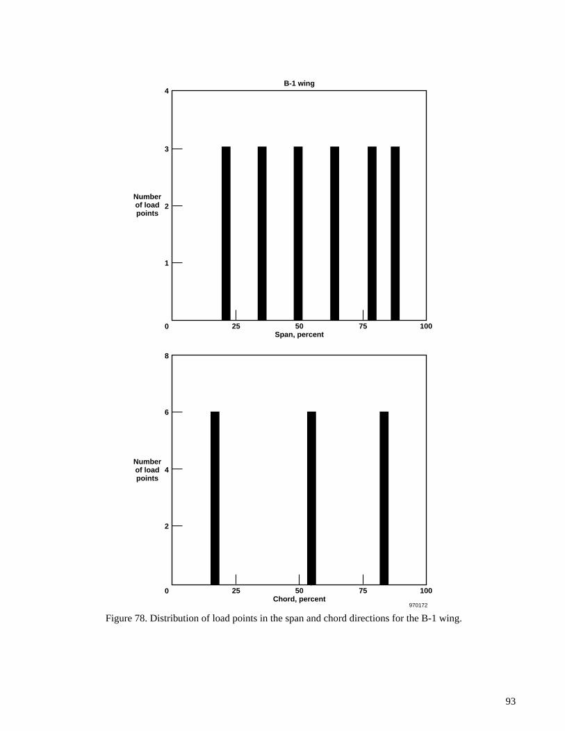
93
25 50Span, percent
B-1 wing
75 100
970172
8
6
4Numberof loadpoints
2
4
3
2Numberof loadpoints
1
0
25 50Chord, percent
75 1000
Figure 78. Distribution of load points in the span and chord directions for the B-1 wing.

400 80 1006020
B-1 strain gage 5307
Two-dimensional plot
Ribbon plot
Wire-frame plot
5307Load points
5312 5310
53075306
Front spar
Rear spar
Span, percent
Chord, percent
56
85
15
970173
40
20
30
Infl
uen
ce c
oef
fici
ent
454035302520151050
LocationStrain-gage Load-point
10
0
100Span, percent
100
0Chord, percent
0
100Span, percent
100
0Chord, percent
Infl
uen
ce c
oef
fici
ent
454035302520151050
Infl
uen
ce c
oef
fici
ent
Strain-gage bridge 5307
Figure 79. Comparison of methods of presenting influence-coefficient plots for a strain-gage bridge located on a B-1wing spar.
Figure 81 shows the most unique aspect of the strain-gage calibration of the B-1 wing. Because the wing wascalibrated using both a distributed-load and a point-load approach, the opportunity arises to compare the resultsobtained from the two methods. A spectrum of flight points is shown in the upper left corner of figure 81 in termsof load factor and Mach number. The five points selected represent a cross section of load distributions andmagnitudes. The high- and low-load factors represent different magnitudes of loads, and the subsonic andsupersonic Mach numbers provide a variation of load distribution in terms of forward and aft center of pressure.The remainder of the figure shows comparisons of computed shear, bending, and torsional loads from equationsdeveloped from both the distributed- and point-load calibrations. Very little difference exists in loads calculatedfrom the two methods. The mean difference in loads calculated from the two methods is less than two percent forall the data shown.
Hypersonic Wing Test Structure
A significant laboratory test article representing part of a delta-wing structure (fig. 2) was fabricatedapproximately two decades ago.22 The general area from which the test article was deduced is shown as the shadedarea on the wing of a hypersonic airplane (fig. 82). Although the hypersonic wing test structure (HWTS) wasprimarily used for high-temperature structures research, studies associated with strain-gage load calibrations were
94
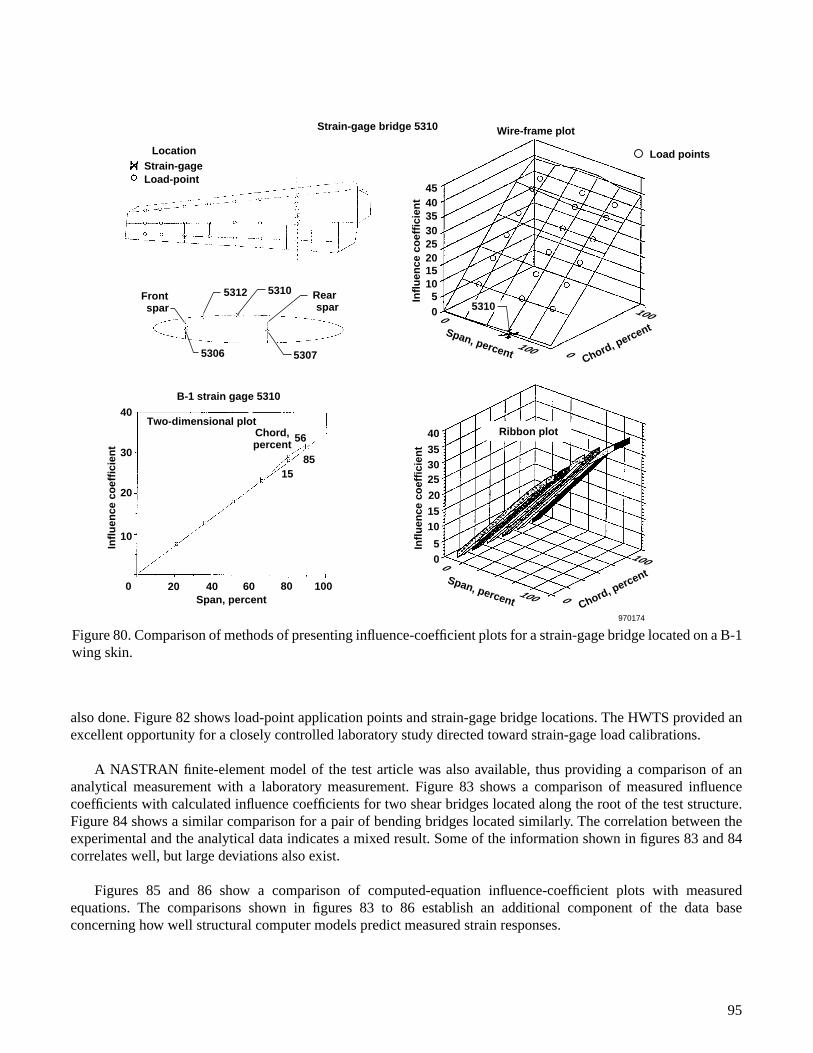
400 80 1006020
B-1 strain gage 5310
Strain-gage bridge 5310
Two-dimensional plotRibbon plot
Wire-frame plot
Load points
5312 5310
53075306
Front spar
Rear spar
Span, percent
Chord, percent
56
8515
970174
40
20
30
Infl
uen
ce c
oef
fici
ent
454035302520151050
LocationStrain-gage Load-point
10
0
100Span, percent
100
0Chord, percent
0
100Span, percent
100
0Chord, percent
Infl
uen
ce c
oef
fici
ent
40
353025
20
1510
50
Infl
uen
ce c
oef
fici
ent
5310
Figure 80. Comparison of methods of presenting influence-coefficient plots for a strain-gage bridge located on a B-1wing skin.
also done. Figure 82 shows load-point application points and strain-gage bridge locations. The HWTS provided anexcellent opportunity for a closely controlled laboratory study directed toward strain-gage load calibrations.
A NASTRAN finite-element model of the test article was also available, thus providing a comparison of ananalytical measurement with a laboratory measurement. Figure 83 shows a comparison of measured influencecoefficients with calculated influence coefficients for two shear bridges located along the root of the test structure.Figure 84 shows a similar comparison for a pair of bending bridges located similarly. The correlation between theexperimental and the analytical data indicates a mixed result. Some of the information shown in figures 83 and 84correlates well, but large deviations also exist.
Figures 85 and 86 show a comparison of computed-equation influence-coefficient plots with measuredequations. The comparisons shown in figures 83 to 86 establish an additional component of the data baseconcerning how well structural computer models predict measured strain responses.
95
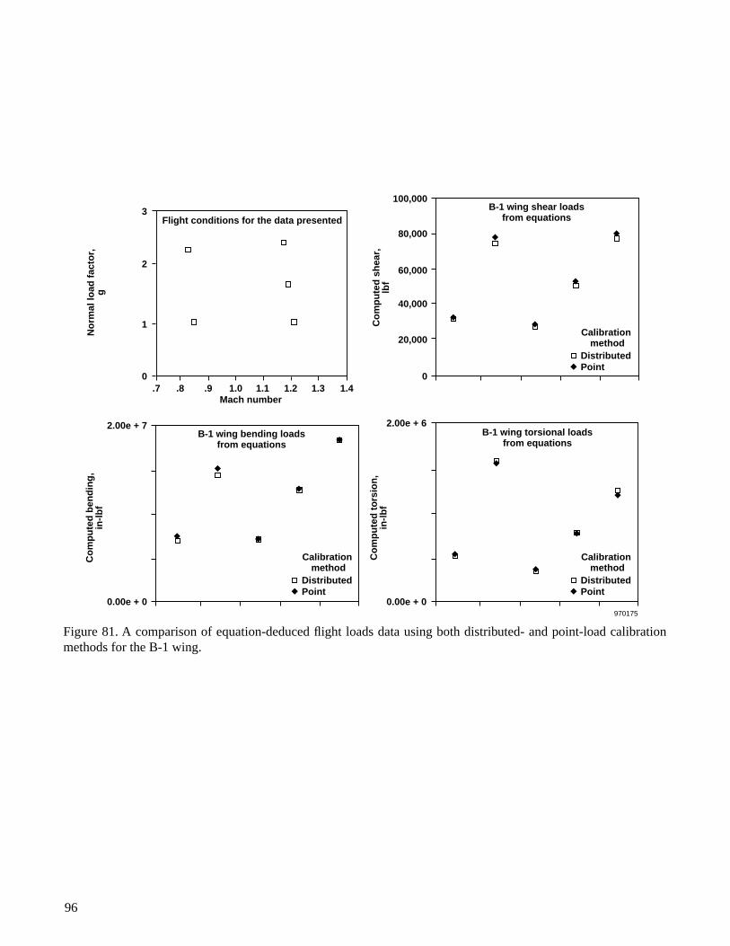
96
.7 .8 .9 1.0 1.1 1.2 1.3 1.4Mach number
Flight conditions for the data presented
B-1 wing bending loadsfrom equations
B-1 wing torsional loadsfrom equations
B-1 wing shear loadsfrom equations
970175
No
rmal
load
fac
tor,
gC
om
pu
ted
ben
din
g,
in-l
bf
Co
mp
ute
d s
hea
r,lb
f
1
0 0
20,000
40,000
60,000
80,000
100,000
2.00e + 7
0.00e + 0
Co
mp
ute
d t
ors
ion
,in
-lb
f
2.00e + 6
0.00e + 0
2
3
Calibration method
DistributedPoint
Calibration method
DistributedPoint
Calibration method
DistributedPoint
Figure 81. A comparison of equation-deduced flight loads data using both distributed- and point-load calibrationmethods for the B-1 wing.

97
Test structure
Torque reference axis
Typical bending bridge
Typical shear bridge
Strain-gagebridge
Wing leading edgeY
1314
1516
1718
12
11
109
8
7
1
2
3
11041105
904905
704705
504505
304305
1041054
5
6
X
20 in.
Chord 100 in.
Span 143 in.
Load pointStrain gage
Wing root
Bending reference axis
38 ft
85°
70°
970176
101 ft
Figure 82. Location of strain gages and load points on the Hypersonic Wing Test Structure.25
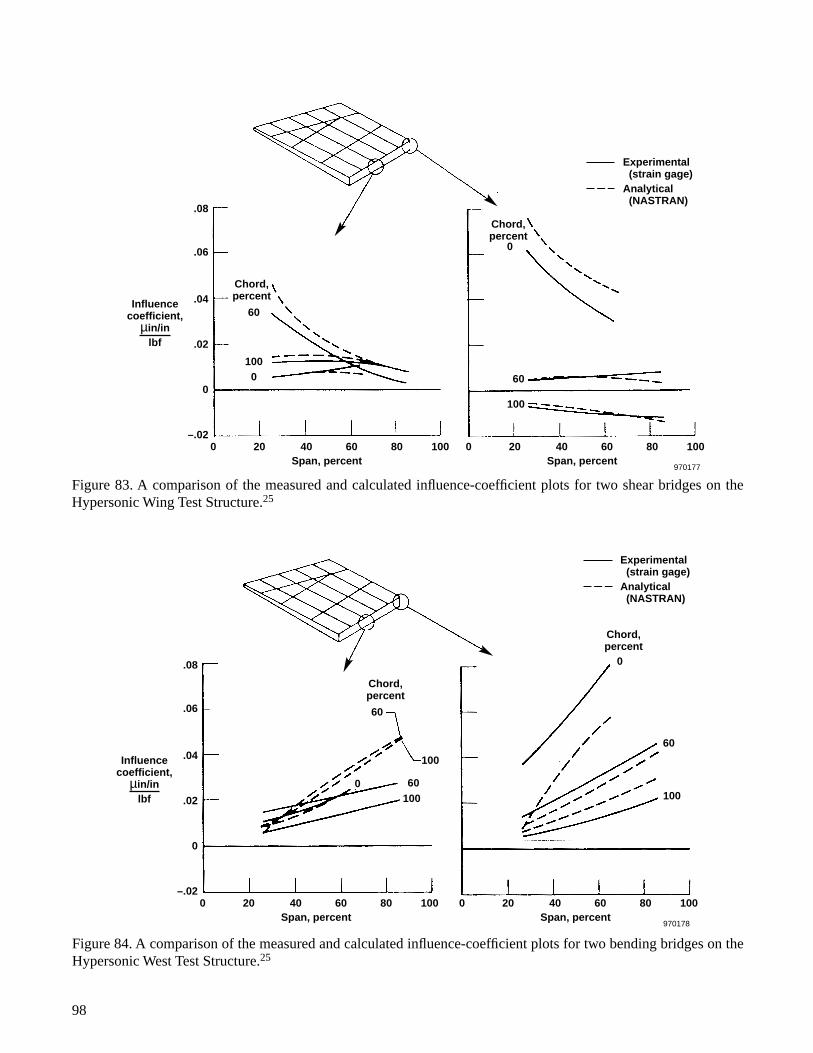
98
.08
.06
.02
0
.04
–.02
Span, percent
Chord, percent
Chord, percent
0 20 40 60 80 100Span, percent
0 20 40 60 80 100
970177
Influence coefficient,
µin/in lbf
60
60
100
100
0
0
Experimental (strain gage) Analytical (NASTRAN)
.08
.06
.02
0
.04
–.02
Span, percent
Chord, percent
Chord, percent
0 20 40 60 80 100Span, percent
0 20 40 60 80 100
970178
Influence coefficient,
µin/in lbf
60
60
60
100
100 1000
0
Experimental (strain gage) Analytical (NASTRAN)
Figure 83. A comparison of the measured and calculated influence-coefficient plots for two shear bridges on theHypersonic Wing Test Structure.25
Figure 84. A comparison of the measured and calculated influence-coefficient plots for two bending bridges on theHypersonic West Test Structure.25
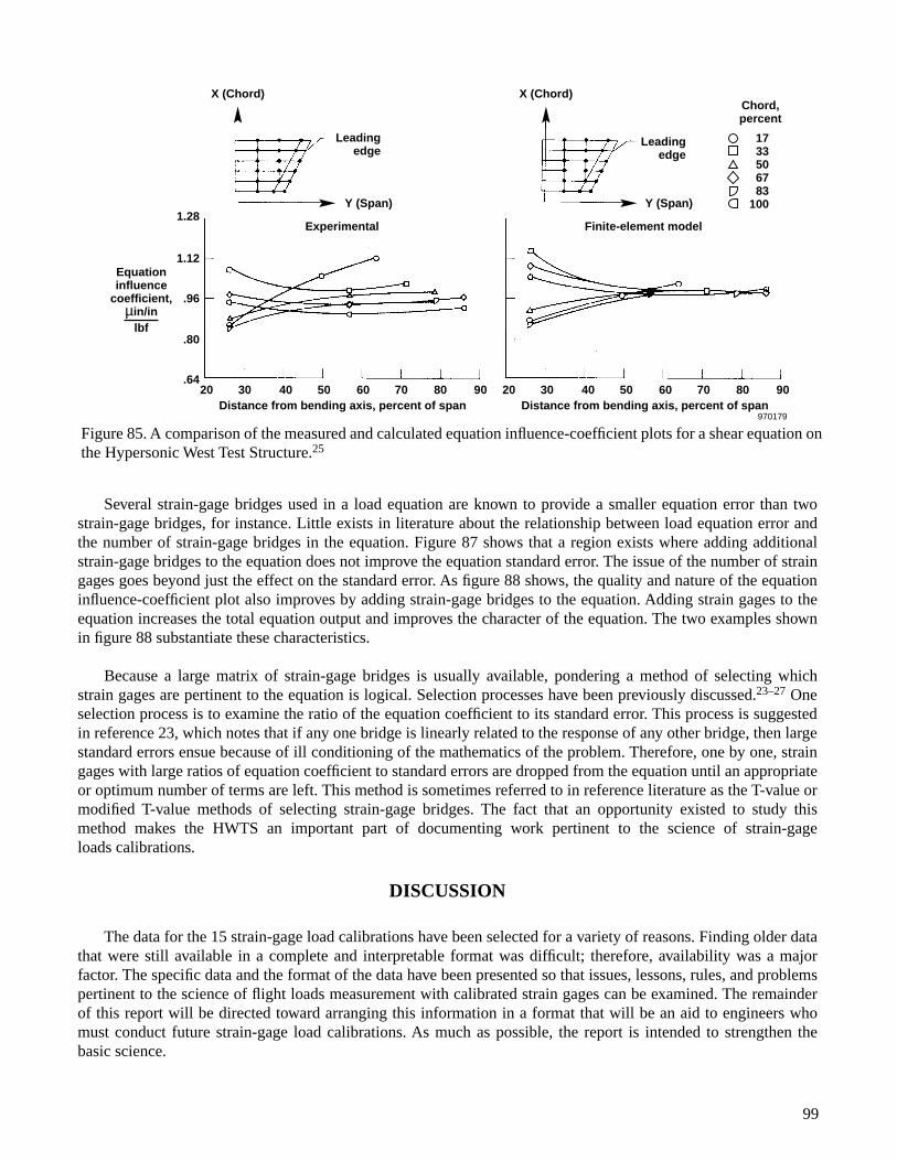
Distance from bending axis, percent of span20 30 908070
Experimental Finite-element model
605040Distance from bending axis, percent of span
20 30 908070605040
970179
Equation influence
coefficient, µin/in
lbf
.64
.80
.96
1.12
1.28
Leading edge
Y (Span)
X (Chord)
Leading edge
Y (Span)
X (Chord)Chord, percent
17 33 50 67 83
100
Figure 85. A comparison of the measured and calculated equation influence-coefficient plots for a shear equation onthe Hypersonic West Test Structure.25
Several strain-gage bridges used in a load equation are known to provide a smaller equation error than twostrain-gage bridges, for instance. Little exists in literature about the relationship between load equation error andthe number of strain-gage bridges in the equation. Figure 87 shows that a region exists where adding additionalstrain-gage bridges to the equation does not improve the equation standard error. The issue of the number of straingages goes beyond just the effect on the standard error. As figure 88 shows, the quality and nature of the equationinfluence-coefficient plot also improves by adding strain-gage bridges to the equation. Adding strain gages to theequation increases the total equation output and improves the character of the equation. The two examples shownin figure 88 substantiate these characteristics.
Because a large matrix of strain-gage bridges is usually available, pondering a method of selecting whichstrain gages are pertinent to the equation is logical. Selection processes have been previously discussed.23–27 Oneselection process is to examine the ratio of the equation coefficient to its standard error. This process is suggestedin reference 23, which notes that if any one bridge is linearly related to the response of any other bridge, then largestandard errors ensue because of ill conditioning of the mathematics of the problem. Therefore, one by one, straingages with large ratios of equation coefficient to standard errors are dropped from the equation until an appropriateor optimum number of terms are left. This method is sometimes referred to in reference literature as the T-value ormodified T-value methods of selecting strain-gage bridges. The fact that an opportunity existed to study thismethod makes the HWTS an important part of documenting work pertinent to the science of strain-gageloads calibrations.
DISCUSSION
The data for the 15 strain-gage load calibrations have been selected for a variety of reasons. Finding older datathat were still available in a complete and interpretable format was difficult; therefore, availability was a majorfactor. The specific data and the format of the data have been presented so that issues, lessons, rules, and problemspertinent to the science of flight loads measurement with calibrated strain gages can be examined. The remainderof this report will be directed toward arranging this information in a format that will be an aid to engineers whomust conduct future strain-gage load calibrations. As much as possible, the report is intended to strengthen thebasic science.
99
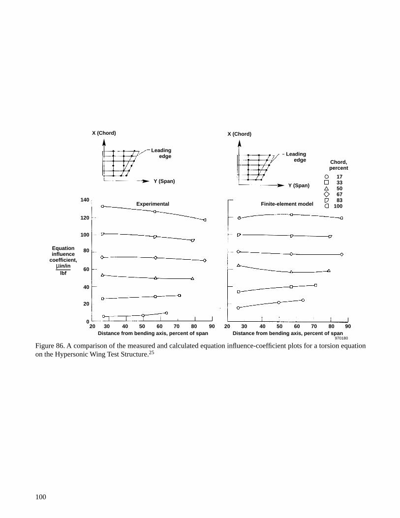
100
Distance from bending axis, percent of span20 30 908070
Experimental Finite-element model
605040Distance from bending axis, percent of span
20 30 908070605040
970180
Equation influence
coefficient, µin/in
lbf
0
20
40
60
80
100
120
140
Leading edge
Y (Span)
X (Chord)
Leading edge
Y (Span)
X (Chord)
Chord, percent
17 33 50 67 83
100
Figure 86. A comparison of the measured and calculated equation influence-coefficient plots for a torsion equationon the Hypersonic Wing Test Structure.25
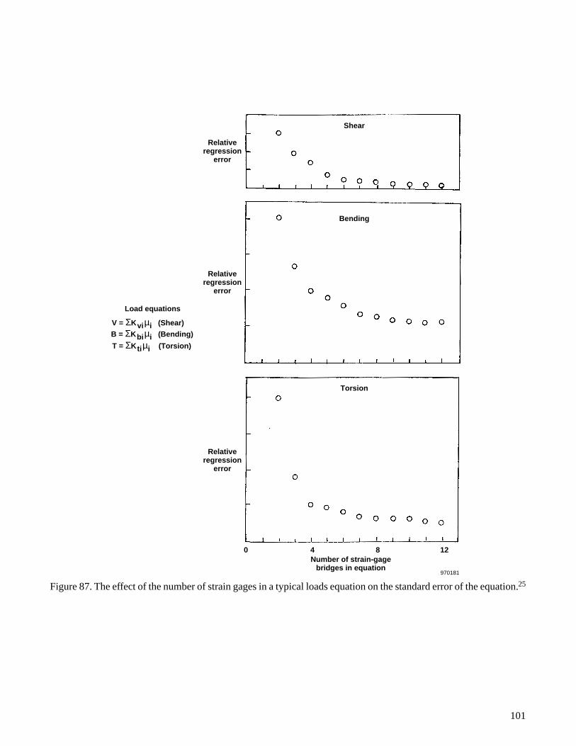
101
970181
0 1284
Relative regression
error
Shear
Bending
Torsion
Relative regression
error
Load equations
V = ΣKviµi (Shear) B = ΣKbiµi (Bending)
T = ΣKtiµi (Torsion)
Relative regression
error
Number of strain-gage bridges in equation
Figure 87. The effect of the number of strain gages in a typical loads equation on the standard error of the equation.25
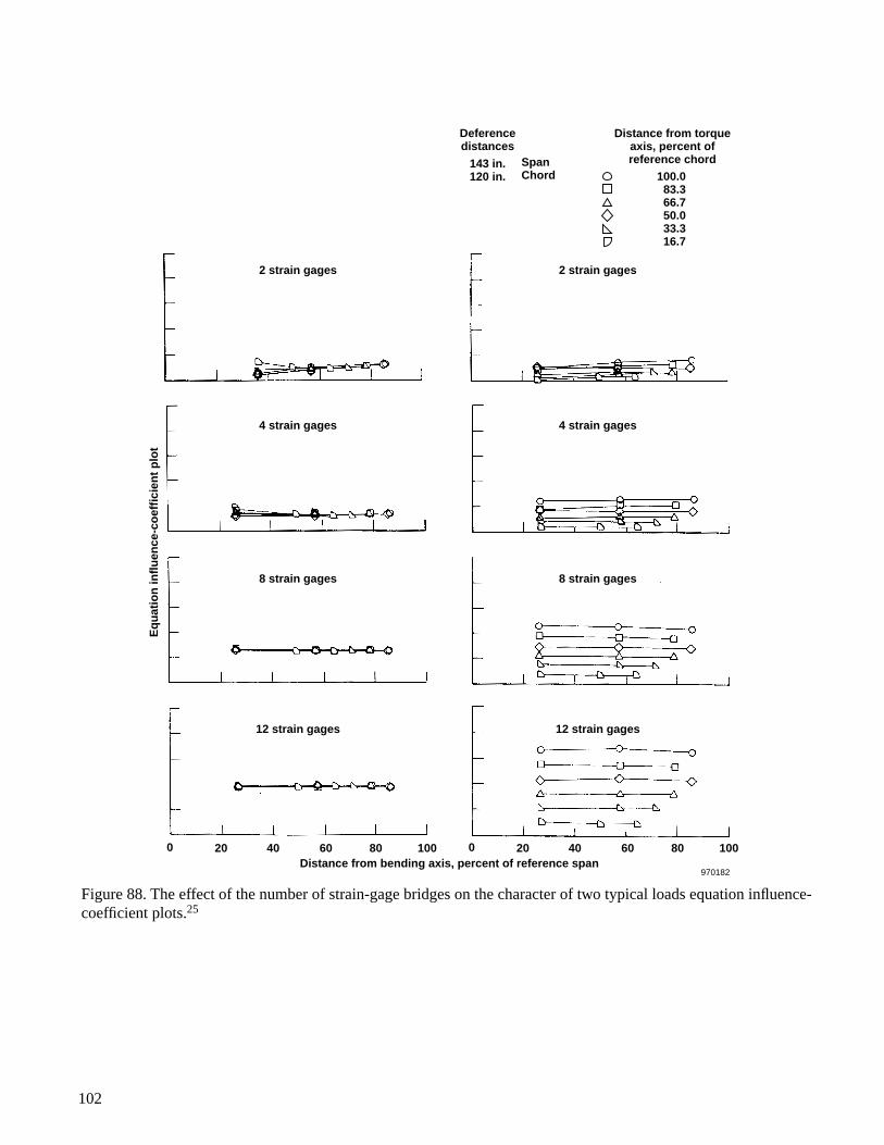
102
970182
0 20 40 60 80 1000 20 40 60 80 100
12 strain gages
Distance from bending axis, percent of reference span
12 strain gages
8 strain gages8 strain gages
4 strain gages4 strain gages
2 strain gages2 strain gages
SpanChord
Deferencedistances
143 in.120 in.
Eq
uat
ion
infl
uen
ce-c
oef
fici
ent
plo
t
Distance from torqueaxis, percent ofreference chord
100.083.366.750.033.316.7
Figure 88. The effect of the number of strain-gage bridges on the character of two typical loads equation influence-coefficient plots.25
The basic science of measuring loads with calibrated strain gages is still evolving and somewhat fluid becausethe approaches must be constantly adapted to changing aircraft technology. The goal of this report is to providemore than just a catalog of information regarding the load calibrations of the various aircraft. Trends, rules, results,presumptions, and directions can be deduced from the data thus far presented that collectively are pertinent todeveloping a science. Although measuring loads with calibrated strain gages is not an exact, well-defined science,approaches certainly exist that are appropriate, and issues exist that should be examined on an individual basis.This section will therefore interpret the information that has thus far been presented with respect to individualaircraft strain-gage calibrations. The format will address specific critical issues in subjects that should form thebasis of a check list for any scientist engaged in measuring loads with strain gages.
Location of Strain Gages
Load measurements are best taken if strain gages are wired in four-active-arm bridges so that the summingeffect of the outputs of four strain gages can be used. Locating shear-sensing bridges on the webs near the shearcenter of the structure minimizes contamination from bending and torsion. Bending bridges should be located onskins or outer caps as far from the neutral axis as possible to maximize the bending outputs. Torsional bridgesshould be located on skins or webs as far from the shear center of the structure as possible, preferably near theplane of the neutral axis, to maximize the torsional response and minimize the bending response. If the location ofthe strain-gage bridge is subjected to temperature changes, the configuration of the strain-gage bridge can be usedto provide temperature compensation. Appendix B provides more details concerning strain-gage bridgeconfigurations. Figure 49 shows detailed locations for an actual strain-gage bridge installation for the T-37B wing.
Selection of Load Points
The point-load calibration of a set of strain gages on a wing- or tail-type structure should include pointloadings in all areas where flight load occur. The spectrum of calibration loads should encompass as much of thespan/chord area as is practical to result in a more complete statistical correlation between the actual flight loadspectrum and the ground load calibration spectrum.
Limitations frequently exist on where loads can be applied to the surface of an aircraft structure. Because loadsare normally applied in some concentrated manner, finding hard points such as spars or ribs that can withstandhigh local stress levels is necessary. The manner in which calibration load points is distributed is greatly influencedby where loads can or cannot be applied to the surface of a wing or tail or other structure. In many respects, thelocation and number of load points is determined more by practicality than by planning.
Number of Strain Gages in Loads Equations
The number of strain gages needed to successfully make a load measurement has always been a subject formuch analysis and evaluation. For some measurements, particularly bending moment, a relatively small number ofterms in the loads equation has yielded very good results. Measuring shear and torsion is clearly a different matter.In order to adequately describe the applied calibration loads, three, four, or even five strain-gage bridges may haveto be included in the equation. Limitations in the number of flight data recording channels is a frequent problemwhen large numbers of strain-gage bridges must be used to acquire the load measurement. Data recordinglimitations may dictate a small number of strain-gage measurements, hence compromising the accuracy of themeasurement. This subject was well covered in figures 87 and 88, where the general trends were studied on alaboratory test structure. Note that the trends and accuracies of the data shown in figures 87 and 88 apply only tothe spectrum of the loads that were applied during the load calibration and that were also used in the derivation ofthe loads equations. Loading conditions outside the spectrum of the load calibration will be discussed in detail in alater section.
103
Derivation of Equations
The conventional approach associated with deriving loads equations has been identified,1 and appendix Fpresents an example of the calculative process. Equations can also be derived using the singular-valueddecomposition approach;2 however, this approach is basically untried on strain-gage load calibrations. If anadvantage to the method of reference 2 exists, it is neither apparent nor demonstrated. Regardless of how theequations are derived, it is important to recognize and be cognizant of the fact that the derivation process leads toan equation that is directed to define the applied loads and not necessarily anything else. Therefore, measuringloads that are not within the spectrum of the calibration loads must be approached with caution.
It is also worthwhile to note that reference 1 suggests two simplified approaches to obtaining loads equations.The first approach is to use n strain gages and apply n load points to the structure and then determine the equationcoefficients exactly by merely solving a set of simultaneous equations of order n. These authors are unaware ofdocumented applications of this method, so evaluating how well this method works is difficult. Another approachis to devise a group of n distributed loads pertinent to the character of the load to be measured. Again, a set ofsimultaneous equations of order n would be solved to obtain the equation coefficients. These authors are alsounaware of any documented examples of this approach.
Automated Strain-Gage Selections
If the structure to be calibrated is complex or highly redundant and a large number of strain-gage bridges areavailable for use in the equations, then choosing the best three, four or five strain-gage bridges for the equation is aformidable task. Automatic selections processes were previously identified.23–27 An additional approach has beendeveloped recently.28 This approach employs genetic algorithms to select an appropriate set of strain-gage bridgesfor the equation. These approaches certainly appear to save considerable work for the load measurement engineer.
In any case where automation is used, spot-checking to make certain that the result appears to correlate withthe physical circumstance of the problem (for instance, the result appears logical) is prudent. In an automatedprocess, a wise approach would be to examine the influence-coefficient plots of the strain-gage bridges that arefinally selected to see if the bridges generally appear to be the combinations that would logically be selectedby inspection.
Load Calibration Relevancy and Load Measurement Error
It is unfortunate that so much emphasis has been given to the handling of the load calibration data. Theaccuracies that are associated with the development of the load equations are only a part of the scenario that leadsto a number that represents load measurement accuracy. Consider a wing in which a load calibration was done byapplying loads to only 20 percent of the wing area, then equations were derived from this 20-percent loadcalibration, and the equation accuracies turned out to be quite good. Further consider the circumstance that inflight, no load occurred on the 20 percent that was calibrated, but the flight loads occurred on the remaining 80percent. Figure 89 shows this extreme example. Although the equations derived from the 20-percent loadcalibration are calculated to be quite good, no reason exists to believe these numbers are relevant to measuring theflight load that occurs on the remaining 80 percent of the wing. Deducing an accuracy in this case would requiresome very far-reaching extrapolation.
This issue was somewhat addressed earlier in this report with the introduction of the relevancy coefficient.This attempt only related the coverage of the calibration loads to the total surface area of the wing or tail that wasto be calibrated. As more load calibrations were introduced, this relevancy coefficient was obviously not thatrelevant, particularly with regard to the load to be measured. Other factors existed that should have been includedin any relevancy measurement, such as aspect ratio, degree of structural redundancy, structural arrangement, and
104
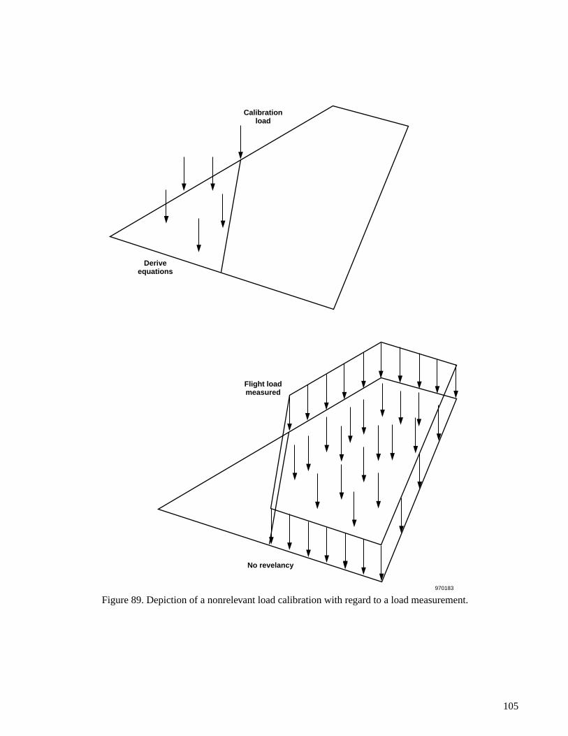
105
Flight loadmeasured
Calibrationload
Deriveequations
No revelancy
970183
Figure 89. Depiction of a nonrelevant load calibration with regard to a load measurement.

the distribution of load. No clearly defined way of establishing a number that represents the accuracy of the loadmeasurement exists. The closest approach to defining such a number would be the application of a distributedcheck load based on some pertinent knowledge of the actual flight load. A distributed check load provides somelink between the equation determined by the load calibration and a relevant distributed check load. If the flight datarecording system is used, then a reasonably good evaluation of the accuracy of the load measurement may result.
Point- and Distributed-Load Calibrations
Strain-gage load calibrations have been successfully accomplished using either point- or distributed-loadingschemes. Other load calibrations have been accomplished using a combination of the two methods in a hybridfashion. Some tendency exists to adopt an approach that is believed to be philosophically the best; however, thehistory of load calibrations indicates that success can be accomplished with any of the point-, distributed-, orhybrid-loading schemes. The approach is more one of applicability rather than philosophical superiority.
Many factors exist that determine the selection process associated with the calibration approach. In recenttimes, the cost of load calibrations has drastically inflated, raising the possibility that load measurements will notbe done. Cost considerations might lead to combining the load calibration with some sort of proof test that mightalso dictate a distributed-load calibration. If the calibration has to be done on the airplane after it is ready to fly, theproblem of reacting large calibration loads always exists. This factor tends to direct the effort toward a discretepoint loading. Also, if the nature of the load to be measured is well known, then a distributed-load calibration withits more restrictive spectrum would seem more appropriate. If the spectrum of possible loads was quite large,however, then the more universal or global point-load approach would seem the most appropriate. In more recentyears, the degree to which an airplane can be loaded has become more restrictive, hence complicating the loadcalibration process. Each strain-gage load calibration, however, must clearly be considered as a unique entity thatrequires an approach tailored to the circumstance.
The B-1 wing was calibrated with both distributed-load and point-load arrays, providing some insight into theissue. The insight is very narrow in perspective, however, because the B-1 wing is a two-cell, high-aspect-ratiostructure that represents one end of the configuration spectrum. In the case of this particular structure, bothcalibration approaches essentially yielded the same results. It cannot be deduced that the same result might beobtained for a different configuration such as a low-aspect-ratio multispar wing. This issue requires additionalinformation to establish generalizations.
Planform Aspect Ratio
Low-aspect-ratio planforms have generally been observed to be more difficult to calibrate than high-aspect-ratio planforms. This effect is likely more appropriately related to the redundancy of the structure than to the shapeof the planform. Structures that have many spars have traditionally resulted in high error calibrations. Thesestructures have also tended to be on the low end of the range of aspect ratios. Wings and tails on the high range ofaspect ratios generally have fewer spars and have better-defined load paths that typically result in lower equationerrors for each load calibration. The effect is most prominent in the measurement of shear. Bending-momentequation errors seem little affected by planform shape; torsion equations are somewhat more affected. Oneanomaly that is an exception to this generalization is the common high-aspect-ratio horizontal tail that frequentlyis attached to the fuselage with a spindle arrangement. Measuring shear on spindle-type structures has historicallybeen very difficult, regardless of the planform shape.
The planform or aspect-ratio effect would not be as noticeable if the number of strain-gage bridges used in theequations were better correlated with the degree of redundancy of the individual structure. A lifting surface withmany spars is usually low in aspect ratio, is highly redundant, and requires many strain-gage bridges in the loadsequations. Therefore, if the number of strain gages in the equations is more closely representative of the degree ofredundancy, then a planform (aspect-ratio) effect would probably not exist.
106

Influence-Coefficient Plots
The influence-coefficient plot is the single most important tool for evaluating the status of a load calibrationand for comparing the character of the calibration with other strain-gage load calibrations. The variation of theinfluence coefficient must be plotted on the vertical axis, with the span plotted on the horizontal axis with constantchord lines in the field. This type of plot can be interpreted in the manner presented in the previous sections ofthis document.
Many calibrations are done without the benefit of influence-coefficient plots. With the capability to automateall parts of a strain-gage load calibration, the opportunity to separate the engineer from the physical problem isextensive. This automation creates the environment for very serious misinterpretations, presumptions, oroversights. Influence-coefficient plots are strongly recommended to be used, and the loads measurement engineershould remain very close to the physical load calibration so that it is apparent that the result is logical.
Because many computer graphics programs are available, influence-coefficient plots were examined from thethree-dimensional point of view. Several cases were presented earlier in this report, and two-dimensionalpresentation was concluded to be more comprehensive than the three-dimensional presentation. This conclusionwas reached because recognizing trends seemed more difficult when the viewer had to address three variables atone time. When addressing the two-dimensional presentation, the viewer could examine two of the variables andthen note the effect of the third variable. This latter approach seemed to provide an easier method of reading thetrends and also seemed more informative.
Local Root Effects
Almost all of the influence-coefficient plots presented in this document exhibit characteristics near the rootthat deviate from the trends that are seen outboard of the root area. These root trends might be characterized asirregularities, nonlinearities, or deviations from the general character of the influence-coefficient plots. The trendsare, in reality, local effects caused by the close proximity of the load to the strain-gage bridges.
Figure 90 shows this effect, where loads A and B can be seen to cause elemental stresses that are different thanthose resulting from load C. What happens is that loads A and B predominately cause bending and shear responsesin terms of the elemental stresses at the strain-gage locations. Load C results in bending, shear, and compressiveresponses at the elemental stress level at the strain-gage locations. For some load points, the strain-gage bridgesrespond to shear, bending, and torsion effects; and for a few other load points, the strain-gage bridges respond toshear, bending, torsion, and compression effects.
The knowledge of the nature of the problem and the knowledge of how to fix the problem can be widelyseparate issues. A calibration load is a very concentrated entity that may bear no resemblance to the way an airload in the same area is distributed to the structure. This lack of resemblance is a problem if the strain-gage bridgehappens to be located in close proximity to the calibration loading jack. Load points that are located remote to thestrain-gage bridge are not capable of causing the compression effect because of the St. Venant effect.19 Therefore,the degree of similarity between the root load point and the air load must somehow be established if any problem-solving is to be accomplished. If the response of the structure to the air load is different from the response of thestructure to the calibration load, then it may be better to discard the root load points from the equation derivationprocess. In other words, the loading at the root area may not be relevant to the measurement of the air loads;therefore, the root loading should not be included in the equation derivation. However, this case is only onescenario. In all probability, the root loading will not be totally irrelevant, in which case a major problem will needto be solved. Concentrated loads on the spars at the root may not be acceptable, in which case distributed loadsthat more closely simulate the actual flight loading at the root may be required. An analytical correction might alsobe applicable. The entire problem of local root effects is one in which considerable effort is required to effect asolution. The mechanics of the local root effects are presented in appendix G in terms of carryover expectations.
107
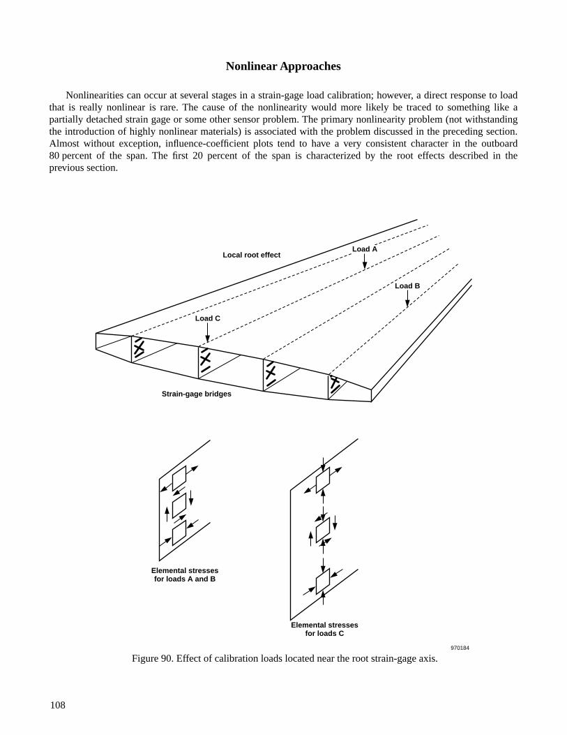
Nonlinear Approaches
Nonlinearities can occur at several stages in a strain-gage load calibration; however, a direct response to loadthat is really nonlinear is rare. The cause of the nonlinearity would more likely be traced to something like apartially detached strain gage or some other sensor problem. The primary nonlinearity problem (not withstandingthe introduction of highly nonlinear materials) is associated with the problem discussed in the preceding section.Almost without exception, influence-coefficient plots tend to have a very consistent character in the outboard80 percent of the span. The first 20 percent of the span is characterized by the root effects described in theprevious section.
108
Local root effect
Elemental stressesfor loads A and B
Elemental stressesfor loads C
Strain-gage bridges
Load B
Load C
970184
Load A
Figure 90. Effect of calibration loads located near the root strain-gage axis.

The difficulty of providing nonlinear definition of the influence-coefficient plots was illustrated quite well infigure 38, where a very severe nonlinearity was evident. The irregularity is so severe in the influence-coefficientplot (fig. 38) that the condition might be more appropriately referred to as a discontinuity, because some of theinformation appears asymptotic. Because applied loads and strain-gage bridge responses are definitely finite,asymptotic information in an influence-coefficient plot obviously cannot exist. Very irregular responses result inunusually complex requirements for any algorithm that would be used to define the influence-coefficient plot.Judgments would have to be made based on solid mechanics theories; hence, a nonlinear approach is thought to beimprudent. An algorithm that could generate the basic influence-coefficient plots from raw data would have to bevery complex and have a large computational requirement.
Computational Strains
As early as 1970, when the YF-12A flight loads efforts were in progress, it became apparent that the powerfulcomputational capabilities associated with evolving finite-element structures computer programs would have greatimpact on strain-gage load calibrations. What role these newly introduced computational capabilities might havewas not clear at that time. In 1970, large structural models were not a realistic goal because of computerlimitations. Small models were available but were not considered sufficiently sophisticated to provide detailedstrains in discrete areas. However, the comparison of computed and measured strain patterns (as shown by theinfluence-coefficient plots and by strains reduced from bridge outputs by the method given in appendix B) wasgenerally quite close for the YF-12A wing. This observation was made in approximately 1970, and at that timereliable computed influence-coefficient plots were recognized as a reality. This result could also be extrapolated todeduce that more could be done in terms of conducting or augmenting the actual load calibration than was possibleat the time.
Later, computational data from the space shuttle and a laboratory test structure (the HWTS) contributed to theagglomerate associated with the ability to compute structural strains from computer models. The correlations ofthe computed influence-coefficient plots with the measured values indicate that, by using a finite-element modelwith sufficient elemental detail, a computational load calibration should be feasible. The primary correlationdeficiency associated with computational efforts was shown to be in the magnitudes of influence-coefficient plots;the shape or character of the influence-coefficient plot correlated well with measurements. The cases where themeasured and calculated values of strain did not correlate well were associated with shear-sensing strain gages.The shear strains associated with direct shear and shear flow are dependent on the thickness of the local structure.The thicknesses used for finite-element models are thought to be incompatible with the actual structure. Thisincompatibility exists because sufficient structural modeling detail does not exist in the areas where the straingages were located.
Figure 91 shows this lack of detail. This figure shows that an actual spar may be a very complex built-upstructure with many doublers. The more efficient the structural design is, the more probable this complexity willexist. The coarser finite element (typical of past models) may very well use one element having one thickness torepresent the actual doublers/webs. This representation means the model does not have a correct thickness at thediscrete location of the strain gage. This incorrect thickness results in the model generating an incorrect shearstrain that obviously will not correlate well with the measurement. This problem can be fixed by using a finite-element model of sufficient detail to provide an accurate thickness at the location of the strain gage. This problemis believed to be resolvable because adequately modeling the local structure is easier with the powerful modelingand computational systems of today.
The need to use a finite-element structural model in association with a load calibration was graphicallyillustrated when the B-2 load calibration was discussed. Surface areas on airplanes that cannot be loadedfrequently exist, such as in the case of the B-2 airplane. However, if a finite-element model of an airplane could beused to develop an analytical load calibration in lieu of a physical loading, the financial savings would be a majorfactor in the overall development cost. The degree to which augmentation, hybridization, and analytics are used incomputational load calibrations is a scenario that has yet to be actualized. The important element is that the timefor computational load calibrations has come.
109
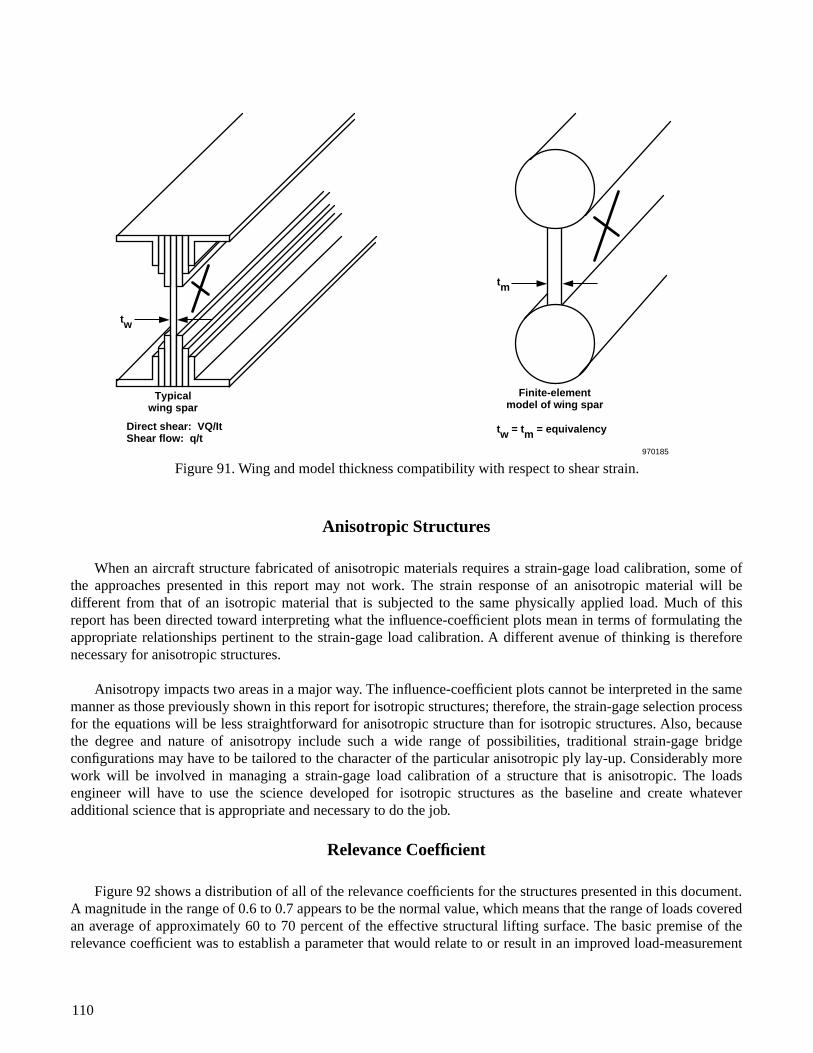
tw
tw = tm = equivalency
tm
Finite-elementmodel of wing spar
Typicalwing spar
Direct shear: VQ/ItShear flow: q/t
970185
Figure 91. Wing and model thickness compatibility with respect to shear strain.
Anisotropic Structures
When an aircraft structure fabricated of anisotropic materials requires a strain-gage load calibration, some ofthe approaches presented in this report may not work. The strain response of an anisotropic material will bedifferent from that of an isotropic material that is subjected to the same physically applied load. Much of thisreport has been directed toward interpreting what the influence-coefficient plots mean in terms of formulating theappropriate relationships pertinent to the strain-gage load calibration. A different avenue of thinking is thereforenecessary for anisotropic structures.
Anisotropy impacts two areas in a major way. The influence-coefficient plots cannot be interpreted in the samemanner as those previously shown in this report for isotropic structures; therefore, the strain-gage selection processfor the equations will be less straightforward for anisotropic structure than for isotropic structures. Also, becausethe degree and nature of anisotropy include such a wide range of possibilities, traditional strain-gage bridgeconfigurations may have to be tailored to the character of the particular anisotropic ply lay-up. Considerably morework will be involved in managing a strain-gage load calibration of a structure that is anisotropic. The loadsengineer will have to use the science developed for isotropic structures as the baseline and create whateveradditional science that is appropriate and necessary to do the job.
Relevance Coefficient
Figure 92 shows a distribution of all of the relevance coefficients for the structures presented in this document.A magnitude in the range of 0.6 to 0.7 appears to be the normal value, which means that the range of loads coveredan average of approximately 60 to 70 percent of the effective structural lifting surface. The basic premise of therelevance coefficient was to establish a parameter that would relate to or result in an improved load-measurement
110
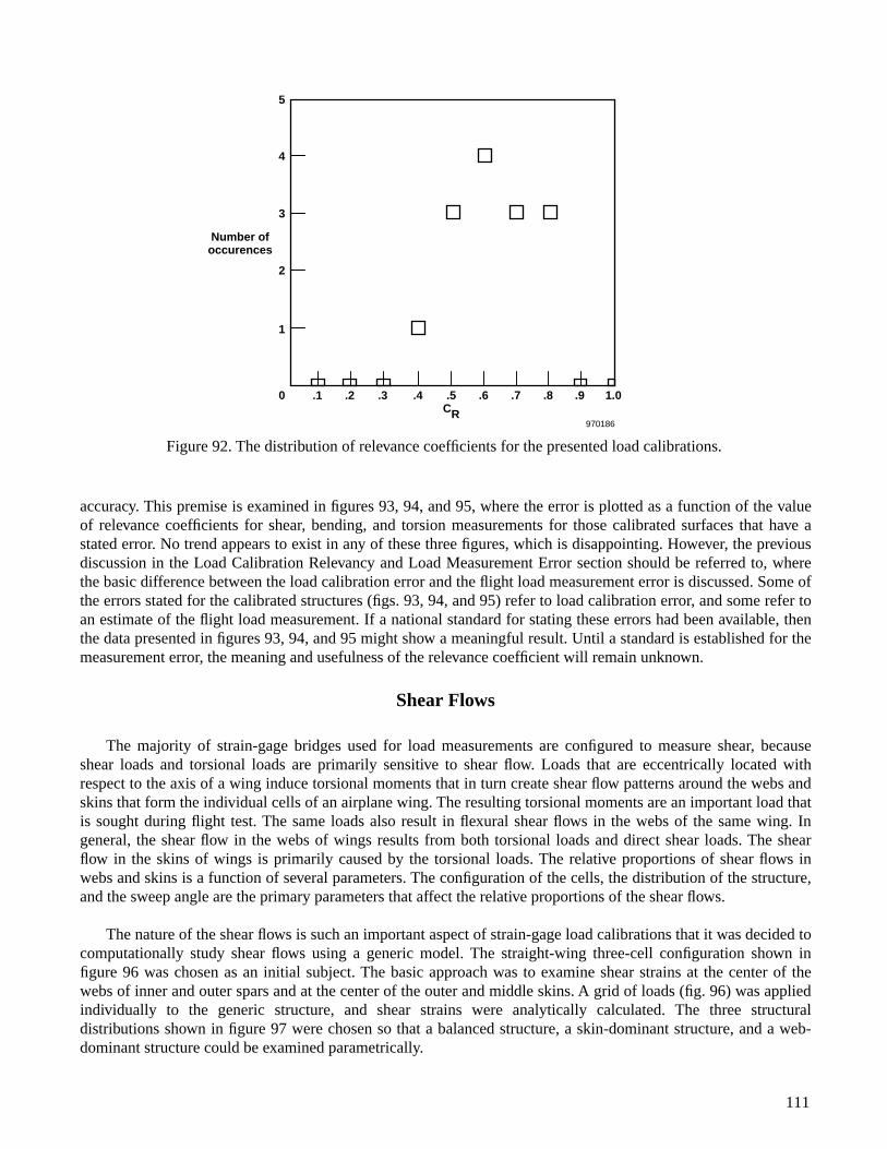
.5CR
.6 .7 .8 .9 1.00
1
2
3
4
5
.1 .2 .3 .4
Number ofoccurences
970186
Figure 92. The distribution of relevance coefficients for the presented load calibrations.
accuracy. This premise is examined in figures 93, 94, and 95, where the error is plotted as a function of the valueof relevance coefficients for shear, bending, and torsion measurements for those calibrated surfaces that have astated error. No trend appears to exist in any of these three figures, which is disappointing. However, the previousdiscussion in the Load Calibration Relevancy and Load Measurement Error section should be referred to, wherethe basic difference between the load calibration error and the flight load measurement error is discussed. Some ofthe errors stated for the calibrated structures (figs. 93, 94, and 95) refer to load calibration error, and some refer toan estimate of the flight load measurement. If a national standard for stating these errors had been available, thenthe data presented in figures 93, 94, and 95 might show a meaningful result. Until a standard is established for themeasurement error, the meaning and usefulness of the relevance coefficient will remain unknown.
Shear Flows
The majority of strain-gage bridges used for load measurements are configured to measure shear, becauseshear loads and torsional loads are primarily sensitive to shear flow. Loads that are eccentrically located withrespect to the axis of a wing induce torsional moments that in turn create shear flow patterns around the webs andskins that form the individual cells of an airplane wing. The resulting torsional moments are an important load thatis sought during flight test. The same loads also result in flexural shear flows in the webs of the same wing. Ingeneral, the shear flow in the webs of wings results from both torsional loads and direct shear loads. The shearflow in the skins of wings is primarily caused by the torsional loads. The relative proportions of shear flows inwebs and skins is a function of several parameters. The configuration of the cells, the distribution of the structure,and the sweep angle are the primary parameters that affect the relative proportions of the shear flows.
The nature of the shear flows is such an important aspect of strain-gage load calibrations that it was decided tocomputationally study shear flows using a generic model. The straight-wing three-cell configuration shown infigure 96 was chosen as an initial subject. The basic approach was to examine shear strains at the center of thewebs of inner and outer spars and at the center of the outer and middle skins. A grid of loads (fig. 96) was appliedindividually to the generic structure, and shear strains were analytically calculated. The three structuraldistributions shown in figure 97 were chosen so that a balanced structure, a skin-dominant structure, and a web-dominant structure could be examined parametrically.
111

112
.5CR
.6 .7 .8 .9 1.00
10
20
30
70
60
50
40
80
.1 .2 .3 .4
Shear error,percent
970187
Figure 93. The variation of the shear equation error with the value of the relevancy coefficient.
.5CR
.6 .7 .8 .9 1.00
10
20
30
70
60
50
40
80
.1 .2 .3 .4
Bendingerror,
percent
970188
Figure 94. The variation of the bending-moment equation error with the value of the relevancy coefficient.
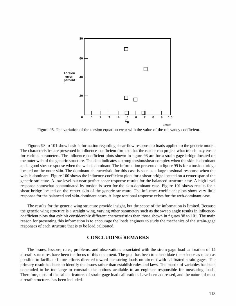
.5CR
.6 .7 .8 .9 1.00
20
60
40
80
.1 .2 .3 .4
Torsionerror,
percent
970189
Figure 95. The variation of the torsion equation error with the value of the relevancy coefficient.
Figures 98 to 101 show basic information regarding shear-flow response to loads applied to the generic model.The characteristics are presented in influence-coefficient form so that the reader can project what trends may ensuefor various parameters. The influence-coefficient plots shown in figure 98 are for a strain-gage bridge located onthe outer web of the generic structure. The data indicates a strong torsion/shear complex when the skin is dominantand a good shear response when the web is dominant. The information presented in figure 99 is for a torsion bridgelocated on the outer skin. The dominant characteristic for this case is seen as a large torsional response when theweb is dominant. Figure 100 shows the influence-coefficient plots for a shear bridge located on a center spar of thegeneric structure. A low-level but near perfect shear response results for the balanced structure case. A high-levelresponse somewhat contaminated by torsion is seen for the skin-dominant case. Figure 101 shows results for ashear bridge located on the center skin of the generic structure. The influence-coefficient plots show very littleresponse for the balanced and skin-dominant cases. A large torsional response exists for the web-dominant case.
The results for the generic wing structure provide insight, but the scope of the information is limited. Becausethe generic wing structure is a straight wing, varying other parameters such as the sweep angle results in influence-coefficient plots that exhibit considerably different characteristics than those shown in figures 98 to 101. The mainreason for presenting this information is to encourage the loads engineer to study the mechanics of the strain-gageresponses of each structure that is to be load calibrated.
CONCLUDING REMARKS
The issues, lessons, rules, problems, and observations associated with the strain-gage load calibration of 14aircraft structures have been the focus of this document. The goal has been to consolidate the science as much aspossible to facilitate future efforts directed toward measuring loads on aircraft with calibrated strain gages. Theprimary result has been to identify the issues rather than establish rules and laws. The matrix of variables has beenconcluded to be too large to constrain the options available to an engineer responsible for measuring loads.Therefore, most of the salient features of strain-gage load calibrations have been addressed, and the nature of mostaircraft structures has been included.
113

114
20 in.
Location of strain-gage bridges
970190
20 in.20 in.
A
BC
D
30 in.
Location of load points
45 in.
Figure 96. Physical description of generic wing used to study shear-flow patterns.
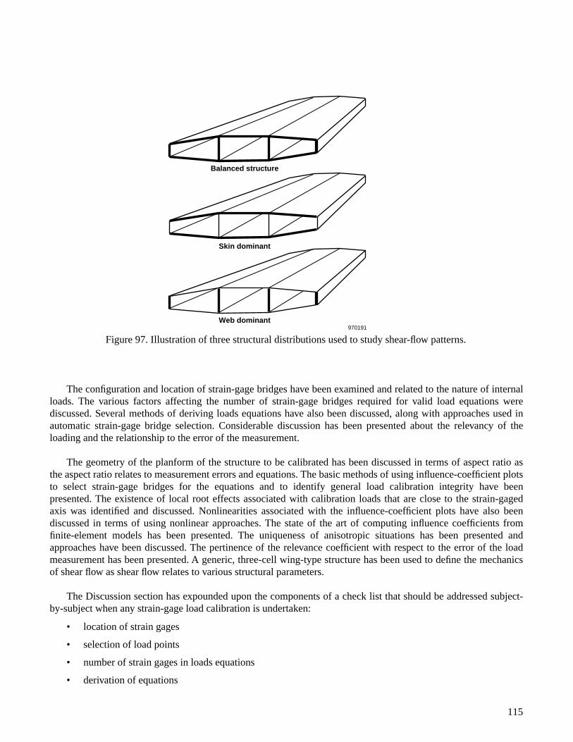
Balanced structure
Skin dominant
Web dominant970191
Figure 97. Illustration of three structural distributions used to study shear-flow patterns.
The configuration and location of strain-gage bridges have been examined and related to the nature of internalloads. The various factors affecting the number of strain-gage bridges required for valid load equations werediscussed. Several methods of deriving loads equations have also been discussed, along with approaches used inautomatic strain-gage bridge selection. Considerable discussion has been presented about the relevancy of theloading and the relationship to the error of the measurement.
The geometry of the planform of the structure to be calibrated has been discussed in terms of aspect ratio asthe aspect ratio relates to measurement errors and equations. The basic methods of using influence-coefficient plotsto select strain-gage bridges for the equations and to identify general load calibration integrity have beenpresented. The existence of local root effects associated with calibration loads that are close to the strain-gagedaxis was identified and discussed. Nonlinearities associated with the influence-coefficient plots have also beendiscussed in terms of using nonlinear approaches. The state of the art of computing influence coefficients fromfinite-element models has been presented. The uniqueness of anisotropic situations has been presented andapproaches have been discussed. The pertinence of the relevance coefficient with respect to the error of the loadmeasurement has been presented. A generic, three-cell wing-type structure has been used to define the mechanicsof shear flow as shear flow relates to various structural parameters.
The Discussion section has expounded upon the components of a check list that should be addressed subject-by-subject when any strain-gage load calibration is undertaken:
• location of strain gages
• selection of load points
• number of strain gages in loads equations
• derivation of equations
115
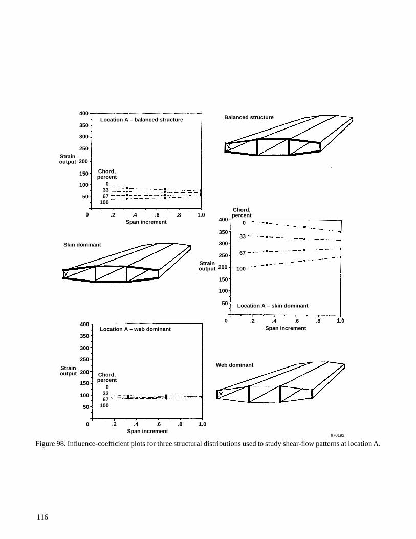
116
Span increment
Chord,percent
Chord,percent
Strainoutput
Web dominant
Skin dominant
Balanced structure
Location A – web dominant
Location A – skin dominant
Location A – balanced structure
.2
03367
100
Chord,percent
03367
100
0
33
67
100
.4 .6 .8 1.00
Span increment.2 .4 .6 .8 1.00
Span increment.2 .4 .6 .8 1.00
50
100
150
0200
250
300
350
400
Strainoutput
50
100
150
200
250
300
350
400
Strainoutput
50
100
150
200
250
300
350
400
970192
Figure 98. Influence-coefficient plots for three structural distributions used to study shear-flow patterns at location A.

117
Span increment
Chord, percent
Shear-strain output
Web dominant
Skin dominant
Balanced structure
Location B – web dominant
Location B – skin dominant
Location B – balanced structure
.2
0
33
67
100
Chord, percent
0 33 67
100
.4 .6 .8 1.00
Span increment.2 .4 .6 .8 1.0
40
20
60
80
0100
120
160
140
180
200
Shear-strain output
40
20
60
80
100
120
160
140
180
200
970193
Span increment.2 .4 .6 .8 1.00
Shear-strain output
40
20
60
80
0100
120
160
140
180
200
0
Chord, percent
0 33 67
100
Figure 99. Influence-coefficient plots for three structural distributions used to study shear-flow patterns at location B.
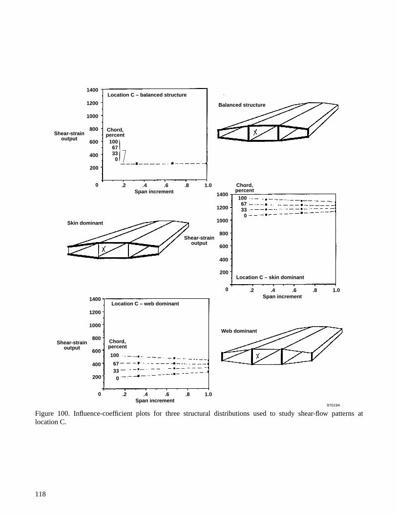
118
Span increment
Chord,percent
Web dominant
Skin dominant
Balanced structure
Location C – web dominant
Location C – skin dominant
Location C – balanced structure
.2
03367
100
Chord,percent
10067330
.4 .6 .8 1.0
Span increment.2 .4 .6 .8 1.0
Span increment.2 .4 .6 .8 1.0
Shear-strainoutput
0
200
400
600
800
1000
1200
1400
970194
Chord,percent10067330
Shear-strainoutput
0
200
400
600
800
1000
1200
1400
Shear-strainoutput
0
200
400
600
800
1000
1200
1400
Figure 100. Influence-coefficient plots for three structural distributions used to study shear-flow patterns atlocation C.
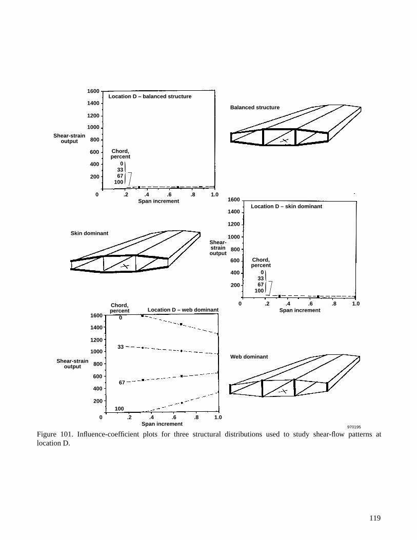
119
Chord, percent
Shear-strain output
Location D – web dominant0
33
67
100
Chord, percent
0 33 67
100
400
200
600
800
1000
1200
1400
1600
Shear- strain output
400
200
600
800
1000
1200
1400
1600
Shear-strain output
400
200
600
800
1000
1200
1400
1600
970195
Chord, percent
0 33 67
100
Span increment.2 .4 .6 .8 1.00
Span increment.2 .4 .6 .8 1.00
Span increment.2 .4 .6 .8 1.00
Web dominant
Skin dominant
Balanced structure
Location D – skin dominant
Location D – balanced structure
Figure 101. Influence-coefficient plots for three structural distributions used to study shear-flow patterns atlocation D.

• automated strain-gage selections
• load calibration relevancy and load measurement error
• point- and distributed-load calibrations
• planform aspect ratio
• influence-coefficient plots
• local root effects
• nonlinear approaches
• computational strains
• anisotropic structures
• relevance coefficient
• shear flows
Some of these subjects will obviously not be pertinent to specific cases. For those subjects that are applicable,however, all aspects of each subject should be considered for impact on the strains of the load calibration andultimately the flight load measurement.
Dryden Flight Research CenterNational Aeronautics and Space AdministrationEdwards, California, January 27, 1997
120

APPENDIX A
SKETCHES OF AIRCRAFT
This appendix contains sketches of twelve aircraft that are subjects considered in the text of this report. Someof the sketches are three-view, and some are plan-view. The purpose of these sketches is to show how some of thestructures interact with the rest of the aircraft.
(a) M2-F2 lifting body.
Figure A-1. Description of aircraft presented in this document.
970196
Station 0
Center-of-gravitylocation
Station 266
Rudders flaredRudders flared
Horizontal referenceline Upper flapsLower flap
9.95 ft(3.033 m)
22.2 ft(6.76 m)
CL
CL
121

(b) X-24A lifting body.
(c) HL-10 lifting body.
Figure A-1. Continued.
970197
Upper rudder
Lower rudder
Upper flap
Lower flap
13.75 ft(4.19 m)
24.50 ft(7.47 m)
7.30 ft(2.23 m)
CL
970198
Elevon flap
Rudder (speed brakes)
Inboard tip fin flap
Outboard tip fin flap
Elevons
15.12 ft(4.61 m)
21.17 ft(6.45 m)
9.60 ft(2.93 m)
122
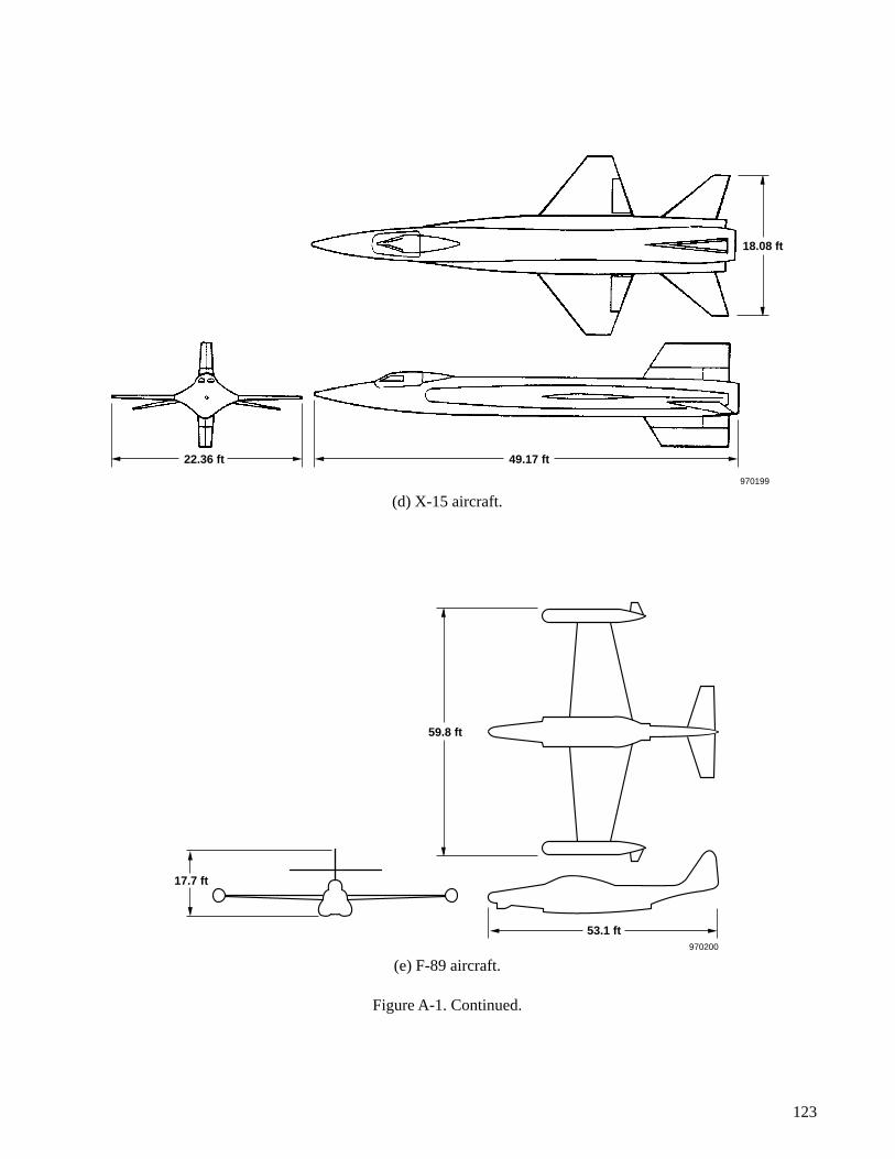
(d) X-15 aircraft.
(e) F-89 aircraft.
Figure A-1. Continued.
18.08 ft
49.17 ft22.36 ft
970199
53.1 ft
59.8 ft
17.7 ft
970200
123

(f) Space Shuttle Orbiter.
(g) T-37B aircraft.
Figure A-1. Continued.
128 ft
78 ft
50 ft
970201
29.2 ft
33.8 ft
9.2 ft
970202
124
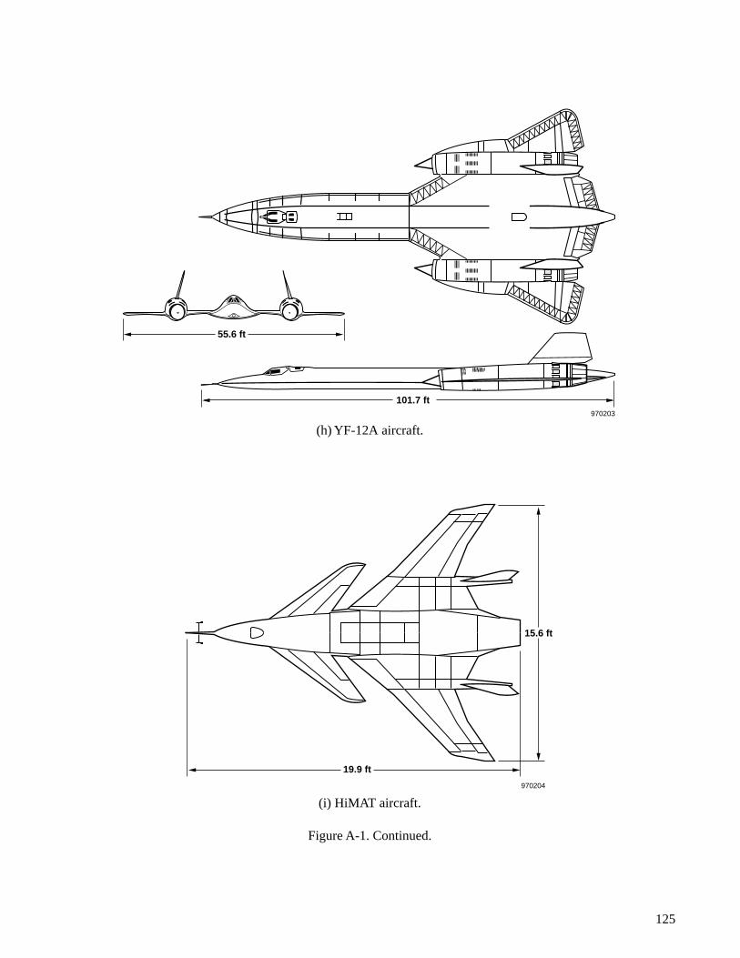
(h) YF-12A aircraft.
(i) HiMAT aircraft.
Figure A-1. Continued.
55.6 ft
101.7 ft970203
15.6 ft
19.9 ft
970204
125
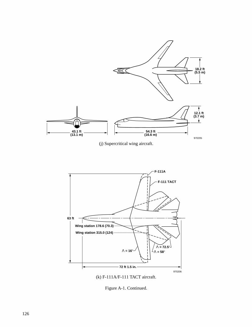
(j) Supercritical wing aircraft.
(k) F-111A/F-111 TACT aircraft.
Figure A-1. Continued.
18.2 ft(5.5 m)
12.1 ft(3.7 m)
43.1 ft(13.1 m)
54.3 ft(16.6 m)
970205
970206
Wing station 178.6 (70.3)
F-111A
F-111 TACT
Wing station 315.0 (124)
Λ = 16°Λ = 72.5°
Λ = 58°
72 ft 1.5 in.
63 ft
126
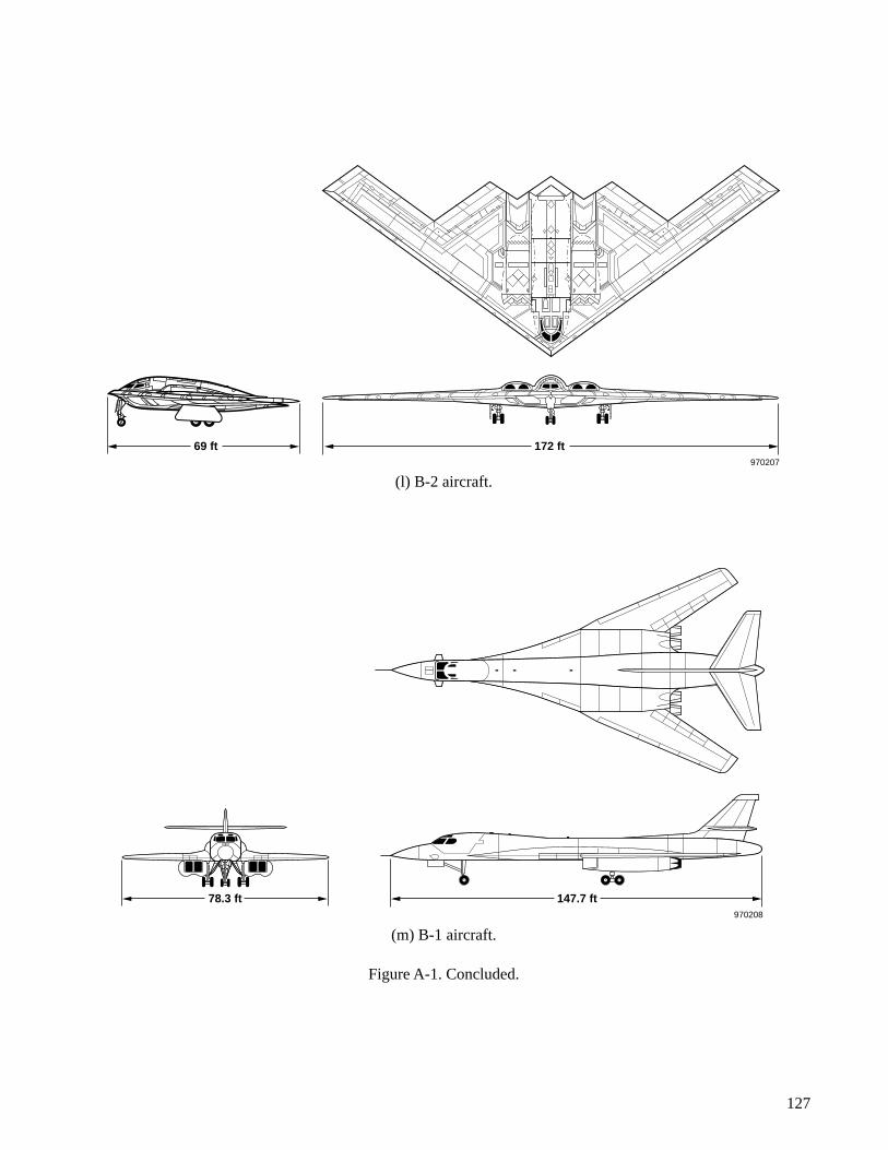
(l) B-2 aircraft.
(m) B-1 aircraft.
Figure A-1. Concluded.
172 ft69 ft970207
147.7 ft78.3 ft970208
127

APPENDIX B
METHOD FOR CONVERTING LABORATORY STRAIN-GAGEBRIDGE DATA TO DISCRETE STRAINS
The basic equation relating strain-gage bridge electrical output with strain is
or
The basic task that needs to be done in estimating the discrete strains is to determine the bridge factor N. Thearray of bending bridges shown at the right are usually wired in the bridge as shown at the left. Note that the signswould be reversed if the bending-moment direction were reversed.
The total effectiveness or the bridge factor is as follows:
where
eo = output voltage
N = bridge factor (dependent upon the stress/strain relationship and the bridge configuration)
GF = gage factor
EX = excitation voltage
eoN4----
GF( ) ε( ) EX( )=
ε4 eo( )
N( ) GF( ) EX( )----------------------------------=
4
3
1
2
3
4
µε− ε
2
1
− µεε
970210.C1
128

Therefore, the discrete bending strain at location 1 is as follows:
The array of strain gages shown at the right is usually wired in the bridge as shown at the left. Note that thesigns of the individual strain gages would reverse if the direction of the shear were reversed.
For a shear bridge, the total effectiveness or the bridge factor is as follows:
All shear strains are presumed to be the same and are considered to be discrete at the center of the strain-gagegrouping. Therefore,
Therefore, the discrete shear strain at the center of the bridge location is as follows:
N Gage 1 Gage 3 Gage 2 Gage 4––+=
N ε1 µε3 µε2– ε4–+=
N 1.00 0.33 0.33 1.00+ + +=
N 2.67=
ε4 eo( )
2.67 GF( ) EX( )------------------------------------=
4
3
1
2 3
4
2
1
− γ/2
− γ/2
γ/2 γ/2
970210.C2
Nγ1
2-----
γ3
2-----
γ2
2-----
γ4
2-----––+=
N 2.0=
γ4 eo( )
2.0 GF( ) EX( )---------------------------------=
129

�
APPENDIX C
PHILOSOPHY OF THE YF-12A FINITE-ELEMENT MODEL
Each spar and rib is idealized as an upper and lower cap connected by a vertical shear web. For example:
The cap area is considered to be the sum of the actual spar cap and a portion of the cover skin. For example:
The amount of cover skin considered effective was determined from tests conducted by the manufacturer. Themodel beam inertias were computed from the magnitude and centroid location of these effective cap areas.For example:
The nacelle spanwise bending was represented by equivalent beams that gave the same bending and shearstiffness as the actual nacelle rings:
AU
AL
Structural idealizationActual structure Bar element
yL
yU
970209.B1
970209.B2
�����
I AUyU 2
A
L
y
L 2
+=
970209.B3
Nacelle
970209.B4
φ δ
Ring
130
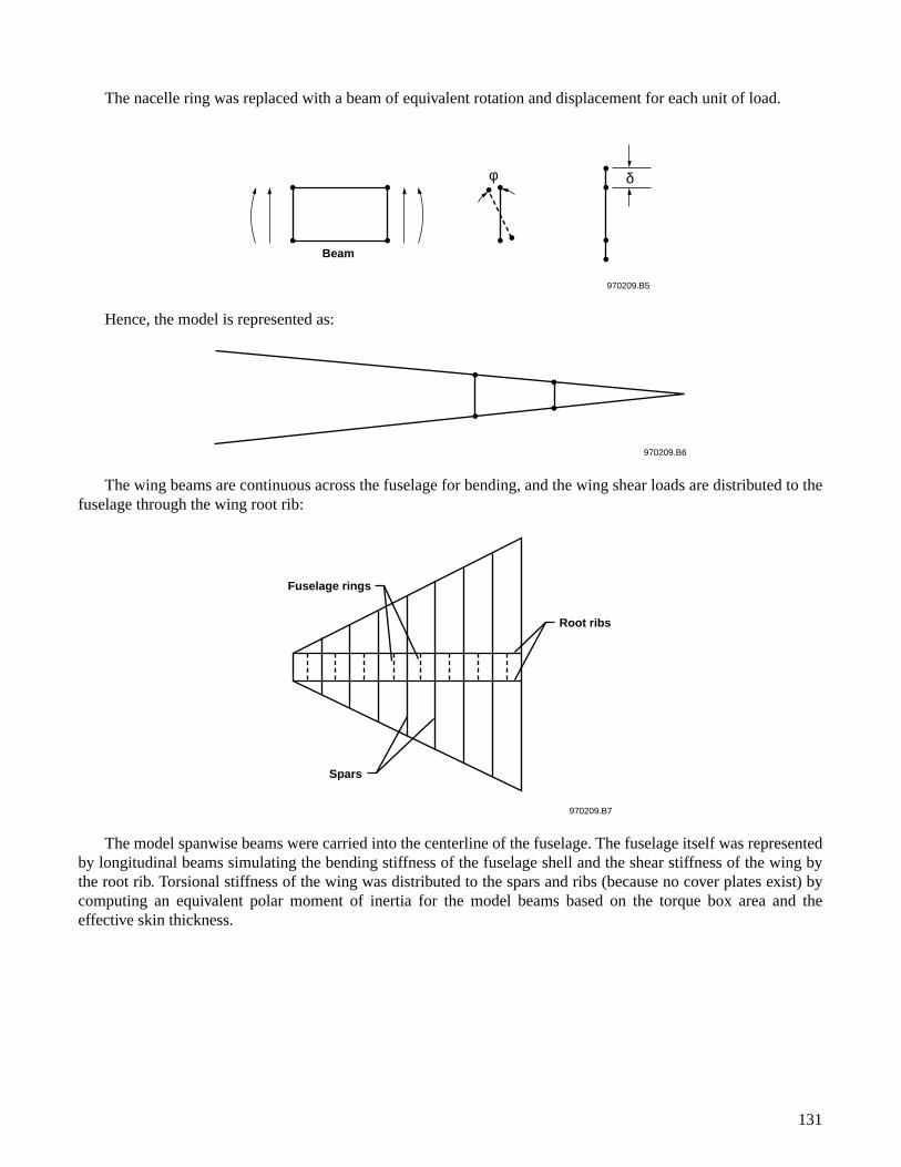
The nacelle ring was replaced with a beam of equivalent rotation and displacement for each unit of load.
Hence, the model is represented as:
The wing beams are continuous across the fuselage for bending, and the wing shear loads are distributed to thefuselage through the wing root rib:
The model spanwise beams were carried into the centerline of the fuselage. The fuselage itself was representedby longitudinal beams simulating the bending stiffness of the fuselage shell and the shear stiffness of the wing bythe root rib. Torsional stiffness of the wing was distributed to the spars and ribs (because no cover plates exist) bycomputing an equivalent polar moment of inertia for the model beams based on the torque box area and theeffective skin thickness.
970209.B5
Beam
φ δ
970209.B6
970209.B7
Spars
Fuselage rings
Root ribs
131

The structure basically looks like this:
The model looks like this:
The stiffness is determined by:
Torsional stiffness of longitudinal beams representing the fuselage and nacelle was determined in asimilar manner.
where A
= area of the cell formed by beams, webs, and upper and lower skins
t
= average skin thickness
p
= perimeter of the cell
970209.B8
970209.B9
J 4 A2 tp---=
970209.B10��
132

APPENDIX D
THE METHOD OF OBTAINING STRAINS FROM THE NASTRAN MODEL
The model is composed of BAR elements. A BAR element can be described by the following sketch:
NASTRAN prints out the following for BAR elements:
• bending moments at both ends
• shears in two planes
• average axial force
• torque about the BAR axis
To decrease the number of elements, the following shortcut was used. If part of the actual structure has fivespars, as shown below:
and if
I
represents the moment of inertia of spars 9, 10, 11, 12, and 13; then a single spar located at 11 can berepresented by the moment of inertia of spar 11 plus one-half the moment of inertia of spars 10 and 12, asshown below:
970211.D1
A/2
A/2
Shear
TorsionAxial force
Bending moment
End A
End B
970211.D2
I9 I10 I11 I12 I13
970211.D3
1/2 I12I111/2 I10
133
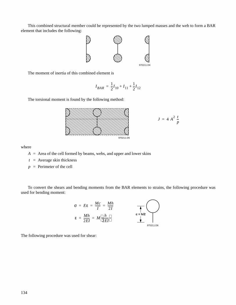
This combined structural member could be represented by the two lumped masses and the web to form a BARelement that includes the following:
The moment of inertia of this combined element is
The torsional moment is found by the following method:
To convert the shears and bending moments from the BAR elements to strains, the following procedure wasused for bending moment:
The following procedure was used for shear:
where
A
= Area of the cell formed by beams, webs, and upper and lower skins
t
= Average skin thickness
p = Perimeter of the cell
970211.D4
�����
���
���
���
���
IBAR12--- I10 I11
12--- I12+ +=
J 4 A2 tp---=
970211.D5
��
���
���
���
σ Eε McI
-------- Mh2I--------= = =
ε Mh2EI--------- M
h2EI---------
= =�970211.D6
c = h/2
134

The shear printed out for the NASTRAN BAR elements represents the lumped element properties; hence, theshear strain is as follows:
τ γGVQIt
--------= =
QA2---
h2---
Ah4
-------= =
I 2A2---
h2---
2 Ah2
4---------= =
τ γGV
Ah4
-------
Ah4
------- 2
t
-----------------= =
τ Vht-----=
γ V2Gth-------------=
��
970211.D7
h
t
c = h/2
A/2
A/2
γ V2Ght-------------=
����
970211.D8
V/2V/4 V/4
135
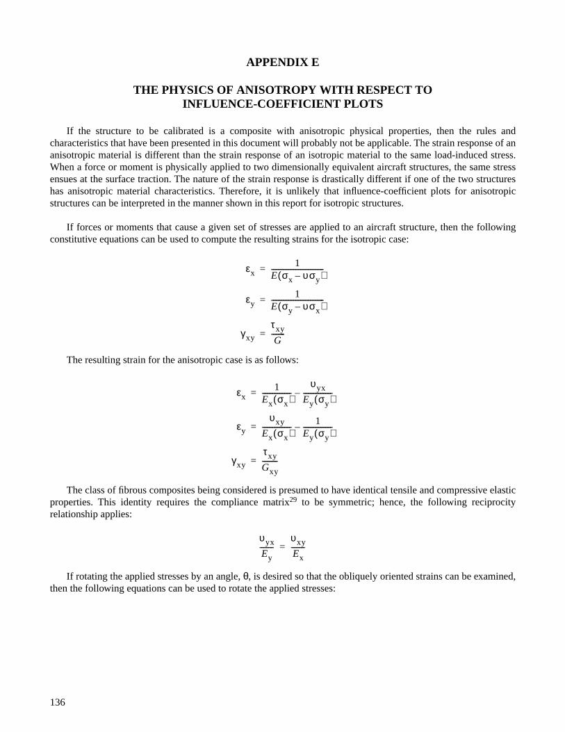
APPENDIX E
THE PHYSICS OF ANISOTROPY WITH RESPECT TOINFLUENCE-COEFFICIENT PLOTS
If the structure to be calibrated is a composite with anisotropic physical properties, then the rules andcharacteristics that have been presented in this document will probably not be applicable. The strain response of ananisotropic material is different than the strain response of an isotropic material to the same load-induced stress.When a force or moment is physically applied to two dimensionally equivalent aircraft structures, the same stressensues at the surface traction. The nature of the strain response is drastically different if one of the two structureshas anisotropic material characteristics. Therefore, it is unlikely that influence-coefficient plots for anisotropicstructures can be interpreted in the manner shown in this report for isotropic structures.
If forces or moments that cause a given set of stresses are applied to an aircraft structure, then the followingconstitutive equations can be used to compute the resulting strains for the isotropic case:
The resulting strain for the anisotropic case is as follows:
The class of fibrous composites being considered is presumed to have identical tensile and compressive elasticproperties. This identity requires the compliance matrix29 to be symmetric; hence, the following reciprocityrelationship applies:
If rotating the applied stresses by an angle, θ, is desired so that the obliquely oriented strains can be examined,then the following equations can be used to rotate the applied stresses:
εx1
E σx υσy–( )-------------------------------=
εy1
E σy υσx–( )-------------------------------=
γxy
τxy
G--------=
εx1
Ex σx( )-----------------
υyx
Ey σy( )-----------------–=
εy
υxy
Ex σx( )----------------- 1
Ey σy( )-----------------–=
γxy
τxy
Gxy---------=
υyx
Ey--------
υxy
Ex--------=
136
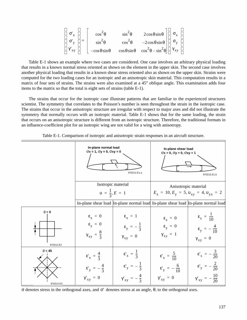
Table E-1 shows an example where two cases are considered. One case involves an arbitrary physical loadingthat results in a known normal stress oriented as shown on the element in the upper skin. The second case involvesanother physical loading that results in a known shear stress oriented also as shown on the upper skin. Strains werecomputed for the two loading cases for an isotropic and an anisotropic skin material. This computation results in amatrix of four sets of strains. The strains were also examined at a 45° oblique angle. This examination adds fouritems to the matrix so that the total is eight sets of strains (table E-1).
The strains that occur for the isotropic case illustrate patterns that are familiar to the experienced structuresscientist. The symmetry that correlates to the Poisson’s number is seen throughout the strain in the isotropic case.The strains that occur in the anisotropic structure are irregular with respect to major axes and did not illustrate thesymmetry that normally occurs with an isotropic material. Table E-1 shows that for the same loading, the strainthat occurs on an anisotropic structure is different from an isotropic structure. Therefore, the traditional formats inan influence-coefficient plot for an isotropic wing are not valid for a wing with anisotropy.
Table E-1. Comparison of isotropic and anisotropic strain responses in an aircraft structure.
Isotropic material Anisotropic material
In-plane shear load In-plane normal load In-plane shear load In-plane normal load
σ denotes stress in the orthogonal axes, and denotes stress at an angle, θ, to the orthogonal axes.
σ'xσ'yγ'xy
cos2θ sin
2θ 2 θ θsincos
sin2θ cos
2θ 2 θ θsincos–
θ θsincos– θ θsincos cos2θ sin
2θ–
σx
σy
γxy
=
In-plane normal loadσx = 1, σy = 0, σxy = 0
970212.E1.a
In-plane shear loadσx = 0, σy = 0, σxy = 1
970212.E1.b
υ 13--- E, 1= = Ex 10 Ey, 5 υxy, 4 υyx, 2= = = =
θ = 0
970212.E2
εx 0=
εy 0=
γxy83---=
εx 1=
εy 13---–=
γxy 0=
εx 0=
εy 0=
γxy 1=
εx110------=
εy 410------–=
γxy 0=
θ = 45
970212.E3
ε'x43---=
ε'y 43---–=
γ'xy 0=
ε'x13---=
ε'y 13---–=
γ'xy 43---–=
ε'x510------=
ε'y 610------–=
γ'xy 0=
ε'x 320------–=
ε'y 220------–=
γ'xy 1020------–=
σ'
137

APPENDIX F
AN ILLUSTRATION OF THE PROCESS OF DERIVING A LOAD EQUATION
This section is included to illustrate how a loads equation can be derived manually. Consider the lifting surfaceshown in figure F-1. The load calibration involves three load points with two strain gages. Using both strain gagesis desired in an equation to describe the applied shear load. For example:
where V is the shear load, µ is the strain-gage output, and β is the equation coefficient to be determined.
The results of the calibration from the table in figure F-1 lead to the following equation:
which can be written as
or
The matrix operations that lead to solving for the coefficients, β, are as follows:1, 30
The inverse of a matrix is the adjoint of the matrix divided by the determinant of the matrix:
V µ303β1 µ311β2+=
1000 0.273β1 0.285β2+=
2000 0.052β1 0.946β2+=
3000 0.054β1 0.909β2+=
1000
2000
3000 0.273 0.285
0.052 0.946
0.054 0.909
β1
β2
=
1
2
3 273 285
52 946
54 909
106– β1
β2
=
V{ } µ[ ] β{ }=
µ[ ] TV{ } µ[ ] T µ[ ] β{ }=
µ[ ] TV{ } µ[ ] T µ[ ]
1–β{ }=
A[ ] 1– 1A[ ]
-------- A ji[ ]=
138

The transpose of the strain-gage output matrix, [µ], is found:
The quantity, [µ]T [µ], is as follows:
A new matrix of the cofactors is constructed:
The transpose of the cofactor matrix is the adjoint:
The determinant of the matrix is as follows:
The inverse is the adjoint divided by the determinant:
Therefore:
273 285
52 946
54 909
T
273 52 54
285 946 909=
273 52 54
285 946 909
273 285
52 946
54 909
80149 176083
176083 1802422=
1802422 176083–
176083– 80149
1802422 176083–
176083– 80149
T1802422 176083–
176083– 80149=
80149 176083
176083 1802422113.4 10
9×= =
1
113.4 109×
---------------------------- 1802422 176100–
176100– 80200
15885 1552–
1552– 70710
9–=
µ[ ] TV{ } µ[ ] T µ[ ]
1–β{ }=
139
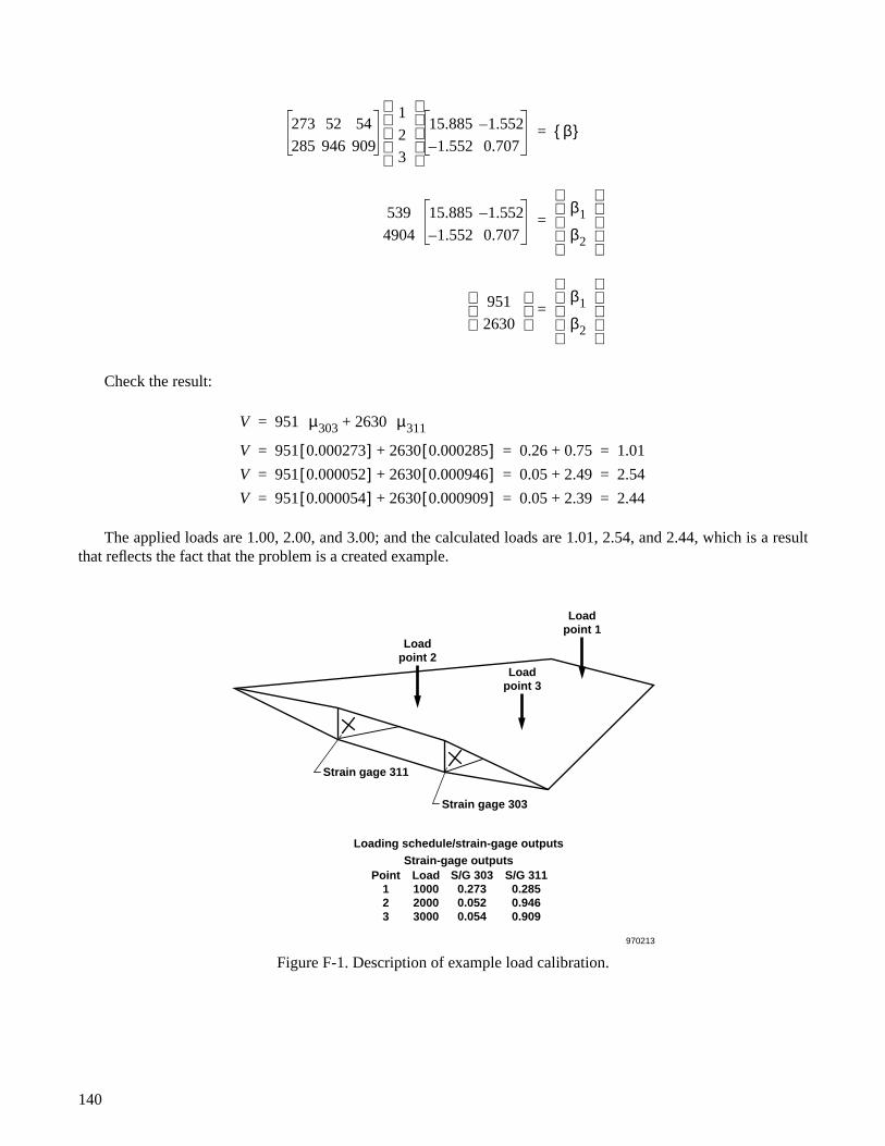
Check the result:
The applied loads are 1.00, 2.00, and 3.00; and the calculated loads are 1.01, 2.54, and 2.44, which is a resultthat reflects the fact that the problem is a created example.
Figure F-1. Description of example load calibration.
273 52 54
285 946 909
1
2
3
15.885 1.552–
1.552– 0.707β{ }=
539
4904
15.885 1.552–
1.552– 0.707
β1
β2
=
951
2630 β1
β2
=
V 951 µ303 2630 µ311+=
V 951 0.000273[ ] 2630 0.000285[ ]+ 0.26 0.75+ 1.01= = =
V 951 0.000052[ ] 2630 0.000946[ ]+ 0.05 2.49+ 2.54= = =
V 951 0.000054[ ] 2630 0.000909[ ]+ 0.05 2.39+ 2.44= = =
Point123
Load100020003000
S/G 3110.2850.9460.909
S/G 3030.2730.0520.054
970213
Strain-gage outputsLoading schedule/strain-gage outputs
Loadpoint 2
Loadpoint 1
Loadpoint 3
Strain gage 303
Strain gage 311
140
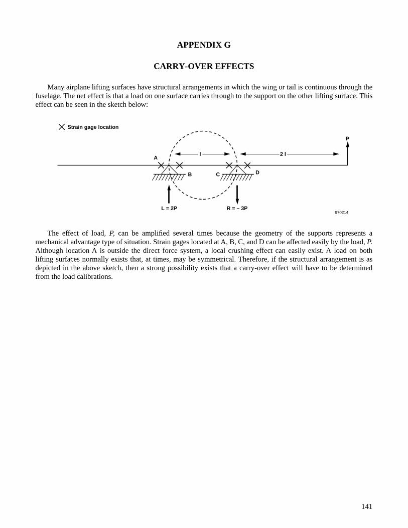
APPENDIX G
CARRY-OVER EFFECTS
Many airplane lifting surfaces have structural arrangements in which the wing or tail is continuous through thefuselage. The net effect is that a load on one surface carries through to the support on the other lifting surface. Thiseffect can be seen in the sketch below:
The effect of load, P, can be amplified several times because the geometry of the supports represents amechanical advantage type of situation. Strain gages located at A, B, C, and D can be affected easily by the load, P.Although location A is outside the direct force system, a local crushing effect can easily exist. A load on bothlifting surfaces normally exists that, at times, may be symmetrical. Therefore, if the structural arrangement is asdepicted in the above sketch, then a strong possibility exists that a carry-over effect will have to be determinedfrom the load calibrations.
l 2 l
R = – 3PL = 2P970214
P
B C D
A
Strain gage location
141

REFERENCES
1 Skopinski, T. H., Aiken, William S., Jr., and Huston, Wilber B., Calibration of Strain-Gage Installations inAircraft Structures for the Measurement of Flight Loads, NACA Report 1178, 1954.
2 Klema, Virginia C. and Laub, Alan J., “The Singular Value Decomposition: Its Computation and SomeApplications,” IEEE Transactions on Automatic Control, vol. AC-25, no. 2, Apr. 1980.
3 DeAngelis, V. Michael, “Strain Gage Loads Measurement Techniques for Hot Structures,” Workshop onCorrelation of Hot Structures Test Data With Analysis, NASA CP-3065, vol. 1, Nov. 1988, pp. 15–XX.
4 Jenkins, Jerald M., Tang, Ming H., and Pearson, George P. E., Vertical-Tail Loads and Control-Surface Hinge-Moment Measurements on the M2-F2 Lifting Body During Initial Subsonic Flight Tests, NASA TM-X-1712, Dec.1968.
5 Tang, Ming H., Sefic, Walter J., and Sheldon, Robert G., Flight-Measured X-24B Fin Loads and ControlSurface Hinge Moments and Correlation with Wind Tunnel Predictions, NASA TM-X-56042, Jan. 1977.
6 Fields, Roger A., A Study of the Accuracy of a Flight-Heating Simulation and Its Effect on Load Measurement,NASA TN-D-5741, Apr. 1970.
7 McCormick, Caleb W., ed., The NASTRAN User’s Manual (Level 15), NASA SP-222(01), 1972.
8 Sefic, Walter J. and Reardon, Lawrence F., “Loads Calibration of the Airplane,” NASA YF-12 Flight LoadsProgram, NASA TM-X-3061, May 1974, pp. 61–107.
9 Jenkins, Jerald M. and Kuhl, Albert E., A Study of the Effect of Radical Load Distributions on Calibrated StrainGage Load Equations, NASA TM-56047, July 1977.
10 Jenkins, Jerald M., Kuhl, Albert E., and Carter, Alan L., “Strain Gage Calibration of a Complex Wing,”Journal of Aircraft, vol. 14, no. 12, Dec. 1977, pp. 1192–1196.
11 National Aeronautics and Space Administration, NASA YF-12 Flight Loads Program, NASA TM-X-3061,May 1974.
12 DeAngelis, V. Michael and Monaghan, Richard C., “HiMAT Strain Gage Loads Calibration and Flight LoadsMeasurement,” Highly Maneuverable Aircraft Technology (U), NASA CP-2412, May 1984, pp. 207–226.
13 Monaghan, Richard C., Description of the HiMAT Tailored Composite Structure and Laboratory MeasuredVehicle Shape Under Load, NASA TM-81354, Feb. 1981.
14 Deets, Dwain A., DeAngelis, V. Michael, and Lux, David P., HiMAT Flight Program: Test Results andProgram Assessment Overview, NASA TM-86725, June 1986.
15 DeAngelis, V. Michael, Wing Panel Loads and Aileron Hinge Moments Measured in Flight on the F-8Supercritical Wing Airplane Including Correlations With Wind Tunnel Data, NASA TM-X-3098, Aug. 1974.
16 DeAngelis, V. Michael and Monaghan, Richard C., Buffet Characteristics of the F-8 Supercritical WingAirplane, NASA TM-56049, Sept. 1977.
17 Coe, Charles F. and Cunningham, Atlee M., Jr., Predictions of F-111 TACT Aircraft Buffet Response andCorrelations of Fluctuating Pressures Measured on Aluminum and Steel Models of the Aircraft, NASA CR-4069,May 1987.
18 Monaghan, Richard C., Flight-Measured Buffet Characteristics of a Supercritical Wing and a ConventionalWing on a Variable-Sweep Airplane, NASA TP-1244, May 1978.
19 Popov, E. P., Mechanics of Materials, Prentice-Hall, Inc., New Jersey, 1952.
142
20 Abbott, Ira H. and Van Doenhoff, Albert E., Theory of Wing Sections: Including a Summary of Airfoil Data,Dover Publications, Inc., New York, 1959.
21 Mock, W. D., Airloads Research Study: Distributed Load Calibration Data, NASA CR-143845, Feb. 1978.
22 Plank, P. P. and Penning, F. A., Hypersonic Wing Test Structure Design, Analysis, and Fabrication, NASACR-127490, Aug. 1973.
23 Hovell, P. B., Webber, D. A., and Roberts, T. A., “The Interpretation of Strain Measurements for Flight LoadDetermination,” C.P. No. 839, Her Majesty’s Stationery Office, London, 1966.
24 Hovell, P. B., Webber, D. A., and Roberts, T. A., “The Use of Calibrated Strain Gauges for Flight LoadDetermination,” C.P. No. 1041, Her Majesty’s Stationery Office, London, 1969.
25 Reardon, Lawrence F., Evaluation of a Strain-Gage Load Calibration on a Low-Aspect-Ratio Wing Structureat Elevated Temperatures, NASA TP-2921, June 1989.
26 Tang, Ming H., “A Modified T-Value Method for Selection of Strain Gages for Measuring Loads,” SESAWestern Regional Strain Gage Committee Fall Meeting, Naval Weapons Center, California, Sept. 16–17, 1980.
27 Tang, Ming H. and Sheldon, Robert G., A Modified T-Value Method for Selection of Strain Gages forMeasuring Loads on a Low Aspect Ratio Wing, NASA TP-1748, Nov. 1980.
28 Nelson, Sigurd A., II, Strain Gage Selection in Loads Equations Using a Genetic Algorithm, NASA CR-4597,Oct. 1994.
29 Whitney, James M., Daniel, Isaac M., and Pipes, R. Byron, Experimental Mechanics of Fiber ReinforcedComposite Materials, Society for Experimental Stress Analysis, Connecticut, 1982.
30 Wylie, C. R., Jr., Advanced Engineering Mathematics, McGraw-Hill Book Company, Inc., New York, 1960.
143

REPORT DOCUMENTATION PAGE Form ApprovedOMB No. 0704-0188
1. AGENCY USE ONLY (Leave blank) 2. REPORT DATE 3. REPORT TYPE AND DATES COVERED
4. TITLE AND SUBTITLE 5. FUNDING NUMBERS
6. AUTHOR(S)
8. PERFORMING ORGANIZATION REPORT NUMBER
7. PERFORMING ORGANIZATION NAME(S) AND ADDRESS(ES)
9. SPONSORING/MONITORING AGENCY NAME(S) AND ADDRESS(ES) 10. SPONSORING/MONITORING AGENCY REPORT NUMBER
11. SUPPLEMENTARY NOTES
12a. DISTRIBUTION/AVAILABILITY STATEMENT 12b. DISTRIBUTION CODE
13. ABSTRACT (Maximum 200 words)
14. SUBJECT TERMS 15. NUMBER OF PAGES
16. PRICE CODE
17. SECURITY CLASSIFICATION OF REPORT
18. SECURITY CLASSIFICATION OF THIS PAGE
19. SECURITY CLASSIFICATION OF ABSTRACT
20. LIMITATION OF ABSTRACT
NSN 7540-01-280-5500 Standard Form 298 (Rev. 2-89)Prescribed by ANSI Std. Z39-18298-102
Public reporting burden for this collection of information is estimated to average 1 hour per response, including the time for reviewing instructions, searching existing data sources, gathering andmaintaining the data needed, and completing and reviewing the collection of information. Send comments regarding this burden estimate or any other aspect of this collection of information,including suggestions for reducing this burden, to Washington Headquarters Services, Directorate for Information Operations and Reports, 1215 Jefferson Davis Highway, Suite 1204, Arlington,VA 22202-4302, and to the Office of Management and Budget, Paperwork Reduction Project (0704-0188), Washington, DC 20503.
.
A Summary of Numerous Strain-Gage Load Calibrations onAircraft Wings and Tails in a Technological Format
WU 505-63-50
Jerald M. Jenkins and V. Michael DeAngelis
NASA Dryden Flight Research CenterP.O. Box 273Edwards, California 93523-0273
H-2154
National Aeronautics and Space AdministrationWashington, DC 20546-0001 NASA TM-4804
Fifteen aircraft structures that were calibrated for flight loads using strain gages are examined. The primarypurpose of this paper is to document important examples of load calibrations on airplanes during the past fourdecades. The emphasis is placed on studying the physical procedures of calibrating strain-gaged structuresand all the supporting analyses and computational techniques that have been used. The results andexperiences obtained from actual data from 14 structures (on 13 airplanes and 1 laboratory test structure) arepresented. This group of structures includes fins, tails, and wings with a wide variety of aspect ratios. Straight-wing, swept-wing, and delta-wing configurations are studied. Some of the structures have skin-dominantconstruction; others are spar-dominant. Anisotropic materials, heat shields, corrugated components,nonorthogonal primary structures, and truss-type structures are particular characteristics that are included.
Anisotropic structure, Flight load, Isotropic structure, Load calibration,Loads measurement, Strain gage
A07
147
Unclassified Unclassified Unclassified Unlimited
July 1997 Technical Memorandum
Available from the NASA Center for AeroSpace Information, 800 Elkridge Landing Road, Linthicum Heights, MD 21090; (301)621-0390
Unclassified—UnlimitedSubject Category 01