Data Mining for Gene Mapping

Data Mining for Gene Mapping

Hannu Toivonen, Paivi Onkamo, Petteri Hintsanen,Evimaria Terzi, and Petteri Sevon

Department of Computer Science andHelsinki Institute of Information Technology

PO Box 26 (Teollisuuskatu 23)FI–00014 University of Helsinki, Finland

E-mail: [email protected], [email protected],[email protected], [email protected],

[email protected]

April 1, 2004

Abstract

Localization of disease susceptibility genes to certain areas in the human genome, or gene

mapping, requires careful analysis of genetic marker data. Gene mapping is often carried

out using a sample of individuals affected by the disease of interest and a sample of healthy

controls. From a data mining perspective, gene mapping can then be cast as a pattern discov-

ery and analysis task: which genetically motivated marker patterns help to separate affected

individuals from healthy ones?

The marker data constitutes haplotypes: a haplotype is a string of genetic markers from

one chromosome. Individuals who share a common ancestor, such as those that have inherited

the disease gene from this individual, potentially share a substring in their haplotypes. Classi-

fication or association analysis of haplotypes is thus one approach to gene mapping. Further,

analyzing the similarities of haplotypes and clustering them can provide insight to genetic rela-

tionships of individuals, to different mutations, and thus to the genetic etiology of the disease.

We describe and illustrate data mining approaches to gene mapping using haplotypes: as-

sociation analysis, similarity analysis, and clustering. The association-based gene mapping

methods have been found to perform well and are being routinely applied in gene mapping

projects.

Keywords: gene mapping, association analysis, haplotype, similarity, clustering

1DRAFT: accepted for publication in 'New Generation of Data Mining Applications'Jozef Zurada and Medo Kantardzic (Eds.), IEEE Press

1 Introduction

Modern biomedical research is uncovering the pathology of diseases once considered to be hope-

lessly complex and incurable. A great deal of this progress can be attributed to gene mapping, i.e.,

localization of disease susceptibility genes to certain areas in the human genome by a combination

of state-of-the-art laboratory and computational methods.

Gene mapping is often based on analysing genetic sequences called haplotypes. (We will re-

view basic concepts of genetics in more detail in the next section; here we aim to give a brief

introduction to the topic of this chapter.) A haplotype is a sparse representation of DNA in (some

part of) one chromosome: only the contents of some selected polymorphic locations of the chro-

mosome are included as symbols in the haplotype. In any particular study, haplotypes are strings

of a fixed length. When inherited from generation to generation, haplotypes are recombined by

cross-overs. This adds variance to the observed haplotypes, and the variance reflects the history

of each haplotype: two haplotypes that have a common ancestor potentially share a segment in

common from that ancestor. In so-called association mapping, geneticists search for segments that

are over-represented in patients of a given disease. The locations of those segments are likely sites

of genes that affect the disease, as the segments are potentially inherited from a common ancestor

together with the gene.

In this chapter we study data mining of haplotypes. A central goal is gene mapping, but we also

consider haplotype similarity and clustering as tools to analyse haplotypes and find some structure

in their relationships. All the methods we propose are based on discovering regularities or similar-

ities in haplotypes; in the case of gene mapping this is done in relationship to the disease/healthy

status of individuals in the study. A big challenge is the large amount of stochasticity in the data:

the recombination process that has led to the observed haplotypes is stochastic, and the disease

status typically correlates only weakly with any single gene.

Association mapping has several alternative formulations as a data mining problem (Section 3).

The first is an extension of association rule mining: the task is to find sets or sequences of polymor-

phic locations and their variants (“attribute-value pairs”) that are associated with the disease status

with a high confidence. A straightforward application of association rules does not work, however.

Three issues need to be addressed: specification of the pattern language, prediction of gene posi-

tion based on discovered patterns, and removing the effect of random associations. An alternative

formulation is classification: use a machine learning method to classify individuals to cases and

controls, and predict a gene to be close to the polymorphic locations used by the classifier.


Association mapping is based on the assumption that several carriers of the gene have inherited

it from a common ancestor and therefore they share haplotype fragments. Similarity measures for

individuals are a useful tool for assessing how closely related patients are and for finding structure

in the haplotypes (Section 4). Clustering, based on similarity measures or directly on genetically

motivated concepts, such as haplotype sharing, can be used to locate groups of individuals that are

likely to share the same genetic etiology (Section 5).

The methods we provide are intended to be used as exploratory tools by geneticists. Like in

any real data mining task, the user’s expertize and insight are in a key role. They are needed

in choosing the methods and parameter values, they are crucial in interpreting the results and in

designing better ways of mining the data. We hope that these tools will help the geneticist to make

useful discoveries.

In Sections 3–5 we will describe how different data mining approaches can be applied on gene

mapping and closely related problems, and illustrate the methods using both synthetic and real

data. Section 6 concludes with a discussion.

2 Genetic concepts

The human genome is organized into 23 different chromosomes,1 each present in every cell as two

homologous copies (Figure 1 A), one from mother and another from father. A chromosome is

a single, giant DNA molecule, consisting of millions of consecutive pairs of nitrogenous bases,

A-T (adenine and thymine), and C-G (cytosine and guanine), which form the well-known double

helix structure with 4-letter alphabet. Most of the DNA has no known functional relevance; only

minority of DNA is estimated to be genes or their regulatory factors (Figure 1 B).

(Figure 1 to be placed approximately here)

The order of the bases and genes is the same from individual to individual, with only minimal

variation: one of the most recent estimates, by Lon Cardon (in his presentation in the Annual

Meeting of The American Society of Human Genetics, 2003) is that there are individual differences

in 1 out of 330 base pairs. This variation inside the genome is utilized as genetic markers (Figure

1 C): the alternative forms of the markers, alleles, can readily be distinguished from each other

using standard laboratory methods (genotyping), and therefore they can be used in comparing

individuals or populations, and in estimating co-occurrence of a disease with certain combination

of marker alleles. A haplotype is a string of alleles in an individual’s chromosome. Haplotypes

1All genetic concepts that are printed in italics when mentioned for the first time can be found in the glossary inTable 1.


can be considered sparse, economic representations of chromosomes, whose focus and density is

set by the location and the density of the marker map used in the study. For genome scans the

marker map covers the whole genome or a full chromosome, for fine mapping studies the markers

are more densely located in a candidate area for a disease susceptibility gene.

A very basic phenomenon in genetics is that of recombination: a pair of homologous chro-

mosomes (represented by haplotypes for a gene mapping study) exchanges genetic material in the

process of gamete production (Figure 2). As a result, a chromosome transmitted from a parent to

an offspring is not an exact copy of either parental chromosomes, but a mosaic of them. Conse-

quently, recombination ensures that between-individual variation is maintained in each generation.

(An a large scale, such as those typically used in gene mapping, the probability of recombination is

approximately constant along the chromosome, and the number of recombinations correlates well

with the physical distance in the chromosome.) Recombination is the key factor for gene mapping:

since it fragments haplotypes, the genealogies of different loci in the genome are different, and this

helps to localize genes.


In association mapping, correlation between the disease or trait (phenotype) and markers is

sought in a sample of affected and healthy individuals from a given population (Figure 3 A). It

is assumed that disease mutations derive from one ancestral chromosome (thus, they are identical

by descent, IBD), where a single mutation occurred a long time ago. (In contrast, alleles which

are chemically identical but cannot be traced to common ancestor are identical by state, IBS.) As

the generations have passed, the disease mutation has been transmitted onward, while recurrent

recombinations have narrowed down the stretch of the ancestral haplotype around the mutation.

Therefore, in the present generation, one observes a haplotype segment overrepresented in the

affected individuals compared to the unaffected (Figure 3 C). There is then linkage disequilibrium

(LD) between the actual disease gene and the surrounding markers. The longer the time which has

passed since the original ancestral mutation, the shorter is the ancestral segment that contains the

mutation.


Association methods are utilized when (1) prior candidate genes exist, or (2) initial linkage to a

genetic region has been observed. Compared to association mapping, linkage analysis, the search

of co-segregation of marker alleles and disease in carefully chosen pedigrees, is the means to get

an initial clue of a position of disease genes (Figure 3 B). Even though linkage analysis is not very

accurate, as only few recombinations can be expected to happen in a chromosome during a couple


of generations, it has proven very useful in locating areas where fine-mapping efforts should be

concentrated. Ultimately, both linkage analysis and association methods search for shared genetic

factors between affected individuals, the difference lying in the size of the “pedigree” concerned

(Figure 3). In this article, we will only consider association mapping.

We will describe novel data mining approaches to association mapping (and the term “gene

mapping” in the rest of this chapter refers to association mapping, not linkage mapping). Due to

historical reasons, the vast majority of gene mapping methodology is based on statistical mod-

elling, in a field that is referred to as ”genetic epidemiology”. The idea of applying data mining

methods to the mapping problem is quite unique, and we are not aware of any similar publications.

We will illustrate our methods with two different data sets.

1. A simulated but realistic data set. The simulated population is an isolate whose age is 20

generations; the marker map is relatively sparse and covers a small chromosome. The final

sample consists of 200 cases and 200 controls. The simulation procedure is described in

more detail in Appendix A.

2. A data set for SLE (systemic lupus erythematosus), where a founder mutation haplotype

has been found very recently [13]. SLE is a rare autoimmune disorder. Its pathogenesis is

polygenic with potential environmental effects. Genes are not yet very well known, though

some candidates have been found by genome scans. We concentrate on a linkage peak area in

chromosome 14 [13, 11]. Both the linkage peak, as well as an association peak were shown

to reside at the same position, in close vicinity of marker D14S1055 at 50.30 cM, which for

the present knowledge is, or is very near to, the actual position of the susceptibility gene.

The proportion of affected individuals actually carrying the particular founder mutation in

chr 14 is on the order of 20%, which is typical for multifactorial diseases.

(Table 1 to be placed approximately here)

3 Gene mapping

3.1 The problem

The goal in gene mapping is to locate disease-predisposing genes. A usual setting consists of

cases and controls: cases are persons that have the disease that is being studied, and controls

are healthy individuals. The existence and importance of a genetic component in the etiology of

the disease has usually already been identified, so the question now is about where the disease


susceptibility (DS) gene or genes are located. Given the haplotypes of cases and controls, the basic

idea in association mapping is to search for genetic patterns that are more common within cases

than controls. Sometimes the trait to be analyzed is quantitative, e.g., blood pressure, rather than

dichotomous case vs. control. In this chapter we consider case–control settings, and will only

briefly outline how to extend the methods for quantitative traits and covariates.

In the following we assume that the gene has been initially mapped to an area on a chromosome.

The area has been saturated with markers and genotyped in a number of individuals. Each individ-

ual in our sample contributes a chromosome pair (one maternal and one paternal chromosome), so

the number of chromosomes in the data is twice the number of individuals. For simplicity, we con-

sider the input data as consisting of a set of disease-associated haplotypes (from the cases) and a set

of control haplotypes (from the controls). It is typical that many or most of the disease-associated

haplotypes do not carry the actual predisposing mutation, and many control haplotypes do carry it.

The association-based gene mapping problem The input consists of a marker map M ��1� � � � �m�,

a set A � �A1� � � � �Ap� of disease-associated haplotypes Ai over map M, and a set C � �C1� � � � �Cq�of control haplotypes Cj over map M. A haplotype H over map M is a vector H � �a1� � � � �am� of

alleles, where ai � Ai and Ai is the set of alleles at marker i. The task is to predict the location of a

disease susceptibility gene on the map M.

3.2 Standard data mining formulations of the gene mapping problem

The problem formulation is vague: it does not say anything about how to predict the gene location.

We next briefly review possible straightforward data mining formulations of the problem.

From a data mining or machine learning view point, gene mapping can be seen as a classifica-

tion problem. This seems obvious, since the input data is readily classified into cases and controls.

The strategy for gene mapping as a classification task is as follows. First, learn to predict whether

a haplotype is a case or a control. Then, by looking at the prediction model, identify the area of

the chromosome that is most important for the classification. The gene is potentially in this area.

While the classification approach may seem tempting, due to the existence of a large variety of

effective and well known classification methods, there are severe problems in any straightforward

application of machine learning methods to this problem. First, the search space is usually huge

with respect to the number of training instances. The number of haplotypes is typically in the

order of tens or hundreds, while the number of markers can be of the same order of much larger.

Machine learning methods would often find over-fit classifiers that perform perfectly with the


available training data, but whose predictions are based on totally irrelevant markers. Further, the

data is extremely noisy. Both cases and controls contain both mutation carrying and non-carrying

haplotypes (class noise), and haplotypes have errors and missing data (attribute noise). Finally,

depending on the classifier, it can be difficult to tell which markers are the most important for

classification.

Another possible approach is to use association rules of the form X �C, where X is a set of

(marker, allele) pairs and C is the case/control status. This is similar to looking for conjunctive

classification patterns, and this approach shares the problems of the classification approach. Al-

though the pattern language is quite restricted and therefore the danger of over-fitting is smaller,

association rules still typically consist of markers that are not related to the mutation. Still another

possibility from machine learning and data mining would be to use feature selection methods to

rank or choose the markers that are most important and thus potentially close to the gene. Again,

in most cases, irrelevant markers would be identified as most important ones.

3.3 Haplotype pattern mining

Like practically any application of data mining or machine learning, the gene mapping problem

requires careful engineering of the types of patterns to be used, i.e., feature construction. The

following three issues need to be addressed:

1. definition of a pattern language that expresses meaningful concepts of the problem at hand,

2. prediction of gene locus based on discovered patterns, and

3. removing the effect of random associations.

We next describe Haplotype Pattern Mining (HPM), a method that has been successfully applied

on gene mapping, and explain how it solves these three issues.

HPM is based on the simple observation that linkage disequilibrium with the DS gene is likely

to be strongest around it and, consequently, the gene locus is likely to be where most of the

strongest associations are. The method looks for haplotype patterns, and predicts the DS locus

to be where strongly disease-associated haplotype patterns are. We give a declarative specifica-

tion of the HPM method after Toivonen et al. [21]; implementation details can be found elsewhere

[21, 22].

Haplotype patterns and disease association We examine linkage disequilibrium by looking

for haplotype patterns that consist of a set of nearby markers, not necessarily consecutive ones.


Given a marker map M � �1� � � � �m�, a haplotype pattern P on M is a vector �p1� � � � � pm�, where

pi � Ai�� for all i�1� i� m, where Ai is the set of alleles at marker i, and * is the ‘don’t care’

symbol. A haplotype pattern P occurs in a given haplotype vector (chromosome) H � �h1� � � � �hm�

if either pi � hi or pi � � for all i�1� i� m.

Example 1 Consider a marker map of 10 markers. The vector

P1 � ��2�5��3��

where 1�2�3� � � � are marker alleles, is an example of a haplotype pattern. This pattern occurs, for

instance, in a chromosome with haplotype �4�2�5�1�3�2�6�4�5�3�.

HPM is based on recognizing disease-associated haplotype patterns that are potentially iden-

tical by descent, i.e., derived from a common ancestor. Gaps are allowed in the patterns to better

accommodate for mutations, errors, missing data, and recombinations.

Example 2 Assume that a continuous chromosomal region including markers 2–5 is inherited

from a common founder by a number of individuals, and that a marker mutation early in the

coalescence history of the disease chromosome has changed the allele in marker 4 for a large

fraction of current chromosomes. The haplotype shared by these individuals can be expressed as a

haplotype pattern of the form of P1 in Example 1.

Example 3 Assume that a continuous chromosomal region including markers 2–5 is inherited

from a common diseased founder by a number of individuals. Errors in genotyping marker 4 may

lead to a situation where a continuous haplotype pattern is not as significantly associated to the

disease status as the one with a gap.

Errors of another type can be introduced in the construction of marker maps, by inferring a

wrong order of markers. Assuming the physical order of markers 4 and 5 is actually the reverse,

situations may occur where pattern P1 is observed for continuous shared regions.

Gaps caused by marker mutations and errors are short, whereas missing information can span

several consecutive markers, depending on how the data has been collected. Long gaps could be

introduced by double recombinations, but they are rare on the genetically short distances where

patterns can be observed in the first place. Since long patterns are not likely to exist, at least not in

significant amounts, it can be useful for performance reasons to restrict the length of the patterns

that are used in gene localization.


Assume a haplotype pattern P � �p1� � � � � pm�. The (genetic) length of P is the maximum

genetic distance (in Morgans) between any two markers i� j with pi �� p j. Gaps are maximal

subsequences of ‘don’t care’ symbols, excluding the tails of the pattern: a gap in P is a contiguous

sequence pu� � � � � pv of alleles, where

1. pi � � for all i�u� i� v (the gap consists of ‘don’t care’ symbols),

2. u � 1 and v � m (the gap is not at either end of the pattern), and

3. pu�1 �� and pv�1 �� (the gap is bounded by alleles, rather than ‘don’t care’ symbols). The

length of the gap is v�u�1.

The HPM algorithm takes as parameters the maximum number and maximum length of gaps, as

well as the maximum length of patterns to be considered.

We use the signed χ2 statistic, denoted χ2, to measure the marker–disease association. A

signed version of the measure is used in order to discriminate disease association from control

association, i.e., from protective haplotypes. The signed χ2 measure χ2�P� of a haplotype pat-

tern P is the standard χ2 measure where the sign is positive if the relative frequency of P is higher

in cases than in controls, and negative otherwise. Given a positive association threshold x, we

say that P is strongly associated with the disease if χ2�P� x. Given the data — markers M,

a set A of disease-associated haplotypes and a set C of control haplotypes on M — and an asso-

ciation threshold x, we denote the collection of all strongly disease-associated patterns by P , i.e.,

P � �P is a haplotype pattern on M � χ2�P� x��If pattern parameters are specified — a maximum genetic length, a maximum number of gaps,

or a maximum length for gaps — the set P is refined by requiring that these additional restrictions

are also fulfilled by the patterns in P . Fisher’s exact test could also be used instead of χ2, especially

if any of the values used in the computation of χ2 are small. Since we do not use χ2 for exact p

value computations, the selection of the test is not critical.

Prediction of gene locus Haplotype patterns close to the DS locus are likely to have stronger

association than haplotypes further away; consequently the locus is likely to be where most of the

strongest associations are. The marker frequency f �i� of marker i (with respect to M�A�C�x as

above) is the number of strongly disease-associated patterns that contain marker i, possibly in a

gap:

f �i� � ��P � �p1� � � � � pm� � P � there exist t � i


and u i such that pt �� pu��

The idea is that each haplotype pattern roughly corresponds to a continuous chromosomal region,

potentially identical by descent, where gaps allow for corruption of marker data. While markers

within gaps are not used in measuring the disease association of the pattern, the whole chromoso-

mal region of the pattern is relevant under the assumption of the region being identical by descent.

The marker frequency gives a score for each marker. On the condition that we assume a DS

gene to be present, e.g., based on linkage analysis, we would predict the gene to be somewhere

close to the markers with largest frequencies. As a point prediction we can simply give the locus of

the most frequent marker: the HPM point prediction of DS gene locus is the location of the marker

i that has maximal frequency f �i�.

This prediction method does not, of course, imply that we assume the DS locus to really overlap

with the marker; we simply predict at the granularity of marker density. Consequently, the optimal

point predictions of our method are within one half of the inter-marker distance from the true loci.

Removing the effect of random associations The frequency-based approach has some poten-

tially severe problems: uneven marker spacing, different allele distributions of markers, unevenly

distributed missing and erroneous data, and background linkage disequilibrium all can change the

observed marker frequencies from what they would be in an ideal situation. This can lead to a

situation where, for instance, a large number of patterns are observed in a certain region due to

larger heterogeneity in and weaker LD between the markers. Some of these patterns can seem sig-

nificant just by random. To avoid these problems we estimate the statistical significance of marker

frequencies. Given a marker i, p�i� is the statistical significance of the frequency f �i� of i under

the null hypothesis that ‘chromosomes are drawn from the same distribution’, i.e., that there is no

gene effect.

Marker significance can be estimated by standard permutation tests. Under the null hypothesis

case and control haplotypes come from the same distribution; by randomly permuting the statuses

of haplotypes we obtain samples from the null distribution. We generate for instance 10 000 such

random permutations and compute the marker frequencies in each of those. The p value p�i� is

then estimated as the fraction of permutations that achieved frequency of at least f �i�.

The HPM significance-based point prediction is the location of the marker i that has minimal

(i.e., highest) significance p�i�. The use of marker significances can be illustrated as follows.

Consider the frequency of a fixed marker as the test statistic. If it is very unlikely that at least that

large a frequency occurs by chance, then it is likely that the DS locus is genetically close to that


marker. The significance-based approach predicts the DS gene to be in the vicinity of the marker

with the smallest p value. Consecutive markers are dependent, and thus a large number of mutually

dependent p values are produced. This is not a problem, however, since we do not use the p values

for hypothesis testing, but only for ranking markers.

3.4 HPM algorithm

In a nutshell, the HPM algorithm is as follows (Figure 4). First, given an association threshold

for the χ2 statistic, a lower bound can be derived for the frequency of strongly disease-associated

haplotype patterns (Step 1). Second, given such a frequency threshold, all patterns exceeding the

threshold can be enumerated efficiently with a fairly straightforward depth-first search method

(Step 2; see [22] for more information about these first two steps).


The strengths of the patterns are then computed, and the the strong ones are used to compute the

marker frequencies f �i� (Steps 3–4). The permutation testing is carried out next (Steps 5–9). The

same set of frequent patterns is reused in every iteration, but the strengths are recomputed based

on the randomized status fields. The final output is a sorted list of markers and their significances.

The first markers in the output have the highest likelihood of being close to the DS gene.

3.5 Extensions of HPM

It is relatively easy to modify HPM to accommodate different kinds of input data. QHPM [20, 16]

is an extension of HPM which can handle quantitative traits and covariates, such as body mass

index, smoking habits, etc. The pattern–trait association is measured via a linear model having the

trait as the response variable and the covariates and an indicator variable for the occurrence of the

pattern as explanatory variables. The significance of the pattern as an explanatory variable can be

tested by comparing the best fit model to the best fit model where the coefficient corresponding to

the pattern is zero. We also replaced marker frequencies with a score function measuring the skew

of the p values of the overlapping patterns.

F-HPM by Zhang and Zhao [23] uses family data instead of independent haplotypes. A family-

based association test proposed by the same authors is used for measuring the pattern–trait associ-

ation.


3.6 Examples

Figure 5 gives graphical representations of the output of HPM on the simulated data set (Ap-

pendix A). The parameters for HPM were set as follows: χ2 threshold was 9, maximum pattern

length was 7 markers, maximum number of gaps was 1, and maximum length of gap was 1 marker.

Permutation tests were carried out with 100,000 iterations. Negated logarithms of p values are

used to illustrate the significance-based predictions, as they are more intuitive than plain p values:

higher values mean stronger association and differences between small p values are more easily

observed. The signal is very strong for the locus on the right, and the number of permutations was

not sufficient to differentiate the markers around the locus. With real data one usually does not

expect to find such a strong signal. The locus on the left is more difficult to detect, and the peak is

off the correct location by 5 cM.


Next, we demonstrate HPM on real Type 1 diabetes data [4, 21] and the SLE data set described

in Section 2. The original diabetes data consisted of affected 385 sib-pair families. There were

25 markers spanning over a 14 Mb region. There are two known genes affecting risk for diabetes,

very close to each other. The genes lie inside the HLA-complex, a region of very high LD, making

the mapping task more difficult. We down-sampled the data to 200 disease-associated and 200

control haplotypes. The same parameters were used as with the simulated data set above. The

result in Figure 6A indicates that HPM is capable of localizing genes even in presence of very

strong background LD.

The SLE data set consisted of 104 disease-associated and 100 control haplotypes. There were

32 markers spread over a 25 cM region. The results (Figure 6B) show suggestive association at

45–50 cM, coinciding with earlier linkage results [13]. Some of the patterns strongly associated

with SLE are listed in Table 2.



HPM has been found to be a valuable tool for narrowing down the region resulting from an

initial linkage analysis. It has been utilized in several disease projects, for instance, asthma and

high IgE [10, 19], SLE [12, 13] glioma [17], and dyslexia (unpublished).


4 Haplotype similarity

Gene mapping, as described above, is indirectly based on finding similar haplotypes among the

affected individuals. In this section we consider explicit similarity measures for haplotypes. For-

mally, given a set G containing n haplotypes with m markers, we want to define a similarity func-

tion sim : G�G � �0�1�, where 0 means total dissimilarity and 1 total similarity. This function

allows us to quantitatively measure a (genetic) similarity between any pair of haplotypes taken

from the set G. The idea is that the similarity is greater if the haplotypes are closely related and

share more of the genome IBD (identical by descent). Depending on the genealogical properties

of the haplotypes G and the exact formulation of sim, this function can be used e.g. to distinguish

between different disease gene mutation carriers or to measure a relationship between haplotypes

or individuals.

4.1 Similarity measures

Given a haplotype pair H1�H2 � G, we compare the alleles at the same locus (marker) within

the haplotypes. By performing this pairwise comparison at every marker, we obtain a similarity

vector �sH1�H2 � �s1� � � � �sm�, where each element si, 1 � i� m, is a result of an allele comparison

at the ith marker: si � 1 if the alleles at ith marker match and si � 0 otherwise. The similarity

vector�sH1�H2 is the base for all our similarity functions.

To begin with, we could simply count the number of 1s in the vector and divide by m, which

yields a similarity function sim�H1�H2� � �∑mi�1 si��m. Observe that 1� sim�H1�H2� is a (normal-

ized) Hamming distance between H1 and H2. The Hamming distance gives an equal weight to ev-

ery match and completely ignores LD (linkage disequilibrium). Therefore it weakly distinguishes

IBD sharing from IBS sharing: it is possible that most of the matching markers are identical by

state and do not reflect true genetic relatedness. (Obviously, the probability that two alleles are

identical by state is higher when the number of different alleles in the corresponding marker is

low. SNP markers only have two alleles, so the probability of IBS sharing is considerably high.)

Longer sequences of matching markers are more likely to be identical by descent due to the LD

between adjacent markers. We consider two simple methods that give more weight for probable

IBD sharing, and one a bit more elaborate method.

Elementary measures First we consider a sliding window technique. Fix a window width w �� . For each marker k in�sH1�H2, we count the amount ak of matching markers covered by the win-


dow starting at the marker: ak � ∑k�w�1i�k si, where si � 0 for i �� 1� � � � �m� (we allow the window

to slide “over the edges” of �sH1�H2). The windowing technique is not sensitive to mismatches in

the middle of the sequence of matches in �sH1�H2. This property makes it robust against genotyp-

ing errors, missing data and point mutations, and gives a smooth weighting for consecutive or

near-consecutive matches.

Now, compute the similarity as a � ∑mk��w�2� a

αk for some constant α 1. The exponent α

gives the desired weight for the possible observed LD: larger values of α put more emphasis

on longer matches. Finally we normalize a by dividing it by the maximum possible score C �

�m�w�1�wα �2∑w�1k�1 kα and let sim�H1�H2� � a�C be the normalized value.

In the second method, we consider each sequence of consecutive matches separately. Let

si� � � � �sk, for 1 � i � k � m, be a substring of �sH1�H2 such that s j � 1 for all i � j � k and si�1 �

sk�1 � 0. Denote by S the set of all such sequences. Let a � ∑s�S �s�α for some α 1, where �s� is

the length of the sequence s. Finally we normalize a so that sim�H1�H2� � a�mα.

As with the sliding window, constant α gives the desired weight for the possible observed

LD. However, unlike the sliding window, this method does not allow any gaps in sequences of

consecutive matches.

Second-order similarity In the second-order similarity (similar in spirit to external similarity

[6]) we do not compare a pair of haplotypes directly to each other, but instead consider their

relations with other haplotypes. The general idea can be described as follows: if two persons share

a lot of (close) relatives, then they probably are (close) relatives, too. We use the above described

elementary similarity measures to estimate which other haplotypes are related and to which degree

with the two haplotypes at hand.

This second-order similarity is useful since the elementary similarity has a large variance due

to the stochasticity of the recombination process and random sharing of alleles. The second order

similarity helps us see more systematic relations between haplotypes. As an extreme example,

suppose that two haplotypes A and B share a DS gene. Assume further that there have been

recombinations very close to the gene in the genealogies of both A and B, but on different sides

of the gene. The haplotypes thus share only few alleles, if any, around the gene locus. The

elementary measures obviously would not consider these haplotypes similar (unless A and B share

a significant amount of alleles somewhere else by chance). If there are other haplotypes carrying

the same mutation, they can help us see A and B as similar. Consider such a mutation carrier C

with its own history of recombinations, all further away from the gene. Then C shares a haplotype


fragment with A (on one side of the gene), another fragment with B (on the other side of the gene),

and has high elementary similarity with both A and B. With several other such haplotypes, we say

that A and B are similar in the second order since they share many closely related haplotypes.

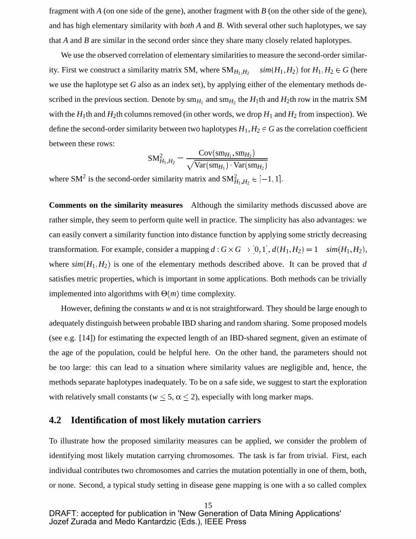
We use the observed correlation of elementary similarities to measure the second-order similar-

ity. First we construct a similarity matrix SM, where SMH1�H2 � sim�H1�H2� for H1�H2 � G (here

we use the haplotype set G also as an index set), by applying either of the elementary methods de-

scribed in the previous section. Denote by smH1 and smH2 the H1th and H2th row in the matrix SM

with the H1th and H2th columns removed (in other words, we drop H1 and H2 from inspection). We

define the second-order similarity between two haplotypes H1�H2 �G as the correlation coefficient

between these rows:

SM2H1�H2

�Cov�smH1�smH2��

Var�smH1� Var�smH2�

where SM2 is the second-order similarity matrix and SM2H1�H2

� ��1�1�.

Comments on the similarity measures Although the similarity methods discussed above are

rather simple, they seem to perform quite well in practice. The simplicity has also advantages: we

can easily convert a similarity function into distance function by applying some strictly decreasing

transformation. For example, consider a mapping d : G�G� �0�1�, d�H1�H2� � 1� sim�H1�H2�,

where sim�H1�H2� is one of the elementary methods described above. It can be proved that d

satisfies metric properties, which is important in some applications. Both methods can be trivially

implemented into algorithms with Θ�m� time complexity.

However, defining the constants w and α is not straightforward. They should be large enough to

adequately distinguish between probable IBD sharing and random sharing. Some proposed models

(see e.g. [14]) for estimating the expected length of an IBD-shared segment, given an estimate of

the age of the population, could be helpful here. On the other hand, the parameters should not

be too large: this can lead to a situation where similarity values are negligible and, hence, the

methods separate haplotypes inadequately. To be on a safe side, we suggest to start the exploration

with relatively small constants (w� 5, α� 2), especially with long marker maps.

4.2 Identification of most likely mutation carriers

To illustrate how the proposed similarity measures can be applied, we consider the problem of

identifying most likely mutation carrying chromosomes. The task is far from trivial. First, each

individual contributes two chromosomes and carries the mutation potentially in one of them, both,

or none. Second, a typical study setting in disease gene mapping is one with a so called complex


disease, where several genes and environmental factors contribute to the disease susceptibility,

and potentially only a small proportion of the chromosomes carry any particular disease mutation.

A single haplotype can carry several mutations, although we restrict our attention to only single

mutation per haplotype for simplicity.

Since carriers sharing a common mutation potentially share several markers IBD around the

mutation locus (depending on the time since the last common ancestor and the density of the

marker map), they are likely to be similar to each other. In addition, any two persons in the dataset

could be related via a common ancestor, so mutation sharing is not the only source of similarity.

Finally, haplotypes can be similar just by chance. We show how the proposed similarity measures

can be applied to distinguish between carrier and non-carrier haplotypes.

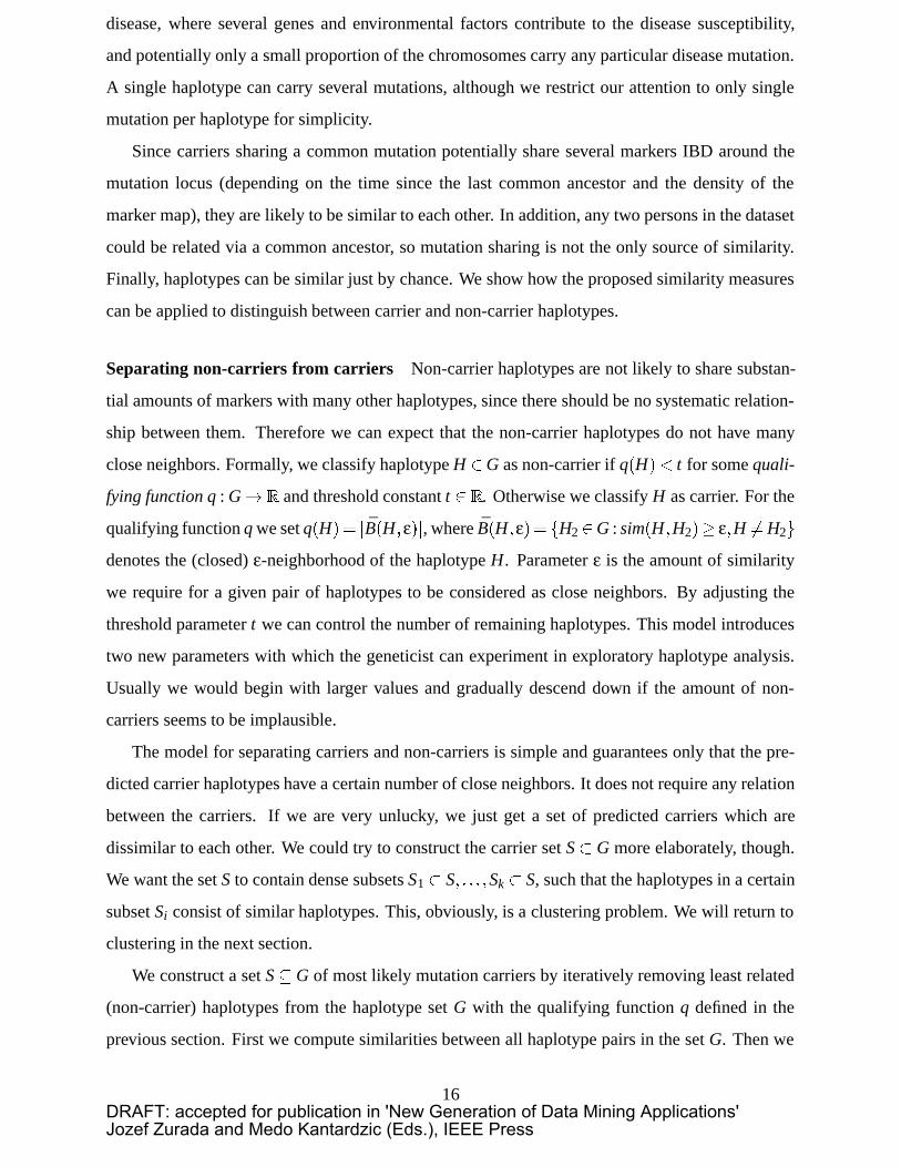
Separating non-carriers from carriers Non-carrier haplotypes are not likely to share substan-

tial amounts of markers with many other haplotypes, since there should be no systematic relation-

ship between them. Therefore we can expect that the non-carrier haplotypes do not have many

close neighbors. Formally, we classify haplotype H �G as non-carrier if q�H�� t for some quali-

fying function q : G� � and threshold constant t � �. Otherwise we classify H as carrier. For the

qualifying function q we set q�H�� B�H�ε��, where B�H�ε�� H2 �G : sim�H�H2� ε�H ��H2�denotes the (closed) ε-neighborhood of the haplotype H. Parameter ε is the amount of similarity

we require for a given pair of haplotypes to be considered as close neighbors. By adjusting the

threshold parameter t we can control the number of remaining haplotypes. This model introduces

two new parameters with which the geneticist can experiment in exploratory haplotype analysis.

Usually we would begin with larger values and gradually descend down if the amount of non-

carriers seems to be implausible.

The model for separating carriers and non-carriers is simple and guarantees only that the pre-

dicted carrier haplotypes have a certain number of close neighbors. It does not require any relation

between the carriers. If we are very unlucky, we just get a set of predicted carriers which are

dissimilar to each other. We could try to construct the carrier set S� G more elaborately, though.

We want the set S to contain dense subsets S1 � S� � � � �Sk � S, such that the haplotypes in a certain

subset Si consist of similar haplotypes. This, obviously, is a clustering problem. We will return to

clustering in the next section.

We construct a set S � G of most likely mutation carriers by iteratively removing least related

(non-carrier) haplotypes from the haplotype set G with the qualifying function q defined in the

previous section. First we compute similarities between all haplotype pairs in the set G. Then we


discard all haplotypes H �G for which q�H�� t with some fairly large threshold and neighborhood

“radius” (for example t � 10 and ε � 0�3 using second-order similarity). If all of the haplotypes get

discarded, we drop the threshold t by one and prune again. If the threshold drops to one (or some

other lower bound we set for the density), we have to adjust ε and try again. We emphasize the

exploratory nature of the process, and the use of genetic insight in the interpretation of the results.

Every haplotype in the set S has a certain number of close neighbors. However, these hap-

lotypes do not need to be close to each other. Therefore we repeat the pruning described above

for the set S without adjusting the parameters t and ε. This removes possible “distant” haplotypes

from the set S. Denote the resulting set of this iteration by S �. If �S�� S��, we are done (now the

set S contains only haplotypes which form group or groups). Otherwise we set S � S � and repeat

the pruning again. Since �S� decreases monotonically, iterating will stop. The subset S might end

up empty, in which case we have to relax threshold parameters.

4.3 Examples

In our first set of examples we use the simulated dataset with 400 haplotypes from affected indi-

viduals with 101 microsatellite markers (Appendix A). There are three different mutations (labeled

M2, M1 and M11) in the sample represented by 58, 56 and 42 carriers. (Two other mutations still

present in the final population are ignored, because they have only one carrier haplotype each.)

Thus, we have four classes, one for each mutation and one for non-carriers.

Similarity between classes First we verify that carriers of a particular mutation are indeed sim-

ilar to each other. This is done by calculating the median similarity with respect to all classes for

each haplotype. We can do this since we know whether a certain haplotype in the simulated dataset

is a carrier or not, and if it is, which mutation the haplotype carries (that is, we know the correct

class for each haplotype). More precisely, for each haplotype H � G and class i we calculate

SHi � medianH2�CiH2 ��H

sim�H�H2�� 1� i� 4�

where C1� � � � �C4 are the known classes.

Figure 7 shows the distributions of SHi . Most of the carrier haplotypes have, as expected,

greater median similarity within their own classes. Observe that most of the non-carrier haplotypes

do not appear to be significantly similar to any group. This is a crucial property when predicting

the carrier haplotypes.



Identification of mutation carriers We next apply the approximation heuristic to the predic-

tion of mutation carriers. For the threshold parameters we set ε � 0�35 and t � 5 and use the

second-order similarity with the sliding window method for measuring pairwise similarities be-

tween haplotypes (with parameters w � 5 and α � 2). Our results are summarized in Table 3.


From the table we observe that all classes are present in the set of predicted carriers. Figure 8

illustrates the trade-off in selectivity. In the figure, two different parameter combinations have been

used and the resulting sets are plotted onto the plane after multidimensional scaling. Although the

heuristic discards a substantial amount of carriers during the process, the remaining haplotypes

are the most likely carriers, and they are likely to show the most distinctive haplotype patterns of

carrier haplotypes. They can be useful, for instance, for developing gene tests before the actual

gene is recognized and can be tested directly.


Structure discovery from real data In our last example we look for similarities in the real

SLE dataset described in Section 2. There are 204 haplotypes with 32 microsatellite markers.

Approximately 8.5 percent of the alleles are missing. When comparing two alleles, the result is

conservatively considered to be a mismatch if either one of the alleles is missing.

We calculate the pairwise similarities with the second-order similarity using the sliding window

method with parameters w � 5 and α � 2. Figure 9A shows the whole dataset plotted onto a plane

with Sammon’s mapping. There are roughly two clusters, which do not seem to be in direct relation

with the disease status or mutation.

To better distinguish the two clusters, we apply the approximation heuristic with parameters

ε � 0�375 and t � 10. This removes exactly half of the haplotypes. We calculate the pairwise sim-

ilarities for the remaining haplotypes with the second order similarity using the same parameters

as before (Figure 9B). The two clusters are now more clearly visible. Again, the disease status or

gene does not seem to have any significance in the separation of the two clusters. The two clusters

suggest, however, that there is some clear structure in the data besides the disease status.



5 Haplotype clustering

5.1 The clustering problem

By haplotype clustering we aim to identify groups of related haplotypes. In some gene mapping

studies, such groups could correspond to different disease gene mutations. Assume a population

isolate created by a relatively small number of founders, constituting the initial generation. Further,

assume that disease susceptibility mutations for the disease of interest have been introduced by few

of the founders. Can the corresponding groups of carriers of different mutations be identified in

the current population? This can be seen as a clustering problem: the goal is to group together

individuals of the present population that have inherited specific regions of their haplotypes from

specific individual founders. Solving this problem can be a rather difficult task, particularly when

the number of generations between the initial and the final population is large, due to the large

number of recombinations and mutations that might have occurred at multiple points.

The problem is closely related to gene mapping, as described in Section 3. The main difference

is that here we are not (directly) concerned with the disease status of the individuals and the goal

is not to separate the control haplotypes from cases but to find groups of haplotypes that have

inherited the mutation from the same ancestral haplotype.

Clustering is the process of grouping together items that have something in common. Several

clustering algorithms exist, most of them requiring a measure of similarity between the items.

(An extensive review of these clustering methods is provided for instance by Jaine et al. [2].)

As discussed in previous sections, a consequence of the recombination process is that haplotypes

that have inherited the mutation from the same ancestor are expected to share some more genetic

material around the mutation locus, and haplotypes that share alleles in consecutive markers should

be considered similar to each other.

This notion of similarity implies that conventional similarity measures are not very useful

for haplotype clustering. Consider for example the three haplotypes shown in Table 4. The

table shows the alleles of 3 haplotypes for markers 1 to 9. By observation the substring 3 4

3 shared by H1 and H2 seems to be genetically significant, since it may correspond to a part

of their common ancestral haplotype. However, using Hamming or Euclidean distance haplo-

type H1 is closer to H2: Hamming Distance�H1�H2� � 6, Hamming Distance�H1�H3� � 4, and

Euclidean Distance�H1�H2� � 36, Euclidean Distance�H1�H3� � 5. Since our goal is to identify

groups of haplotypes that share a mutation from a common ancestor, the clustering method should

be based on some groupwise similarity measure rather than any pairwise similarity.



5.2 Conceptual clustering

Conceptual clustering builds on the idea that the clustering algorithm should produce clusters that

can be described in a given language L , which has been designed to express meaningful concepts of

the domain. (For a discussion of the properties of certain conceptual clustering models, see [18].)

In the sequel we describe the concept language as well as the haplotype clustering algorithms that

have been employed for automating the concept formulation.

The concept language Given that the haplotypes of each cluster are expected to be genetically

related by sharing a gene inherited from a common ancestor, the concept language should con-

sist of expressions that describe shared haplotype segments. Due to recombinations, however, it

is possible that there is no single haplotype segment that would both match most haplotypes in

the (desired) cluster as well as separate them from other haplotypes. Therefore, the clusters are

described by disjunctions of partially overlapping haplotype segments; the goal is that they are

likely to be parts of ancestral haplotypes shared by subgroups. Disjunctions allow flexibility that

is necessary due to different recombination histories of different haplotypes, while the overlap po-

tentially contains the disease susceptibility gene, and also makes it more likely that the haplotypes

within a cluster are related.

Example 4 An example of a disjunctive concept is shown in Table 5. Marker 88 is probably

inherited from a common ancestor, while the different haplotype segments to the left and to the

right are the results of different recombinations.


Formally, the haplotype cluster description language L consists of disjunctions of overlapping

haplotype segments of the form

i : ai�ai�1� � � � �ai�Li or j : a j�a j�1� � � � �a j�L j or k : ak�ak�1� � � � �ak�Lk�

where i� j� ��k are markers, ai is an allele at marker i, Li�Lj� ��Lk are the lengths of the disjuncts,

and there is at least one shared marker h such that i� h� i�Li� j� h� j�Lj� � � � �k� h� k�Lk.

The clustering algorithm As potential disjuncts in the concepts, we consider all haplotype seg-

ments shared by more than a certain number of haplotypes. For finding them efficiently we use a


slight modification of the Apriori algorithm [1]. We then focus on each marker in turn and con-

struct the subsegment containment lattice of overlapping segments that contain this marker. An

abstract description of the haplotype clustering algorithm is given in Figure 10, while some details

of the method are discussed in the sequel.


At each marker i we construct the containment lattice LAT Ti of the frequent haplotype segments

that contain i (Steps 1 and 2). In the first level of LAT Ti we consider the alleles that are frequent in

this marker and use them as the roots of the lattice. In the next level segments of length two that

contain the marker-allele pairs already considered in the previous level are considered, and so on.

The use of the lattice structure biologically motivated. Assuming that a locus is identical by de-

scent in the given haplotypes then the genealogy of the locus is tree-shaped. Under the assumption

of no marker mutations this tree is contained in the haplotype segment lattice build at that locus.

These assumptions are not fully realistic: first, only an unknown subset of haplotypes shares a mu-

tation of interest IBD; second, marker mutations, errors and missing data can violate the second

assumption. Since we do not know the loci of interest, we build a lattice at every marker locus

to obtain a representative collection of lattices that potentially contain an interesting genealogy.

Unlike the unknown trees, the lattices are unique and efficient to construct.

We next select the most promising lattices, based on the number of nodes in each lattice. Close

to the mutation locus, where several haplotypes have segments identical by descend, the lattices

are expected to have more internal nodes when compared to the number of internal nodes in the

lattices for loci where sharing is by state only.

Finally we select the most descriptive nodes of each lattice and output their disjunction as a

cluster description (Steps 4–6). We assign a score for each node (haplotype segment) of the lattice,

based on the heuristic that a haplotype segment constitutes a good description if it is long and

frequent. These two requirements of a good description are combined in the following heuristic,

recursive definition of the score of a node n:

score�n� �

�n.length�n.frequency� if n is a leaf

∑u�children of �n�u.frequencyn.frequency � score�u� if n is not a leaf.

For each lattice LAT Tj � S LAT T the score of the nodes in the lattice is evaluated and the nodes

are sorted in decreasing order. A disjunction of the p highest scoring haplotype segments is used

as the cluster description. There can be logically redundant disjuncts in a cluster description; we

have decided to keep them since they may be informative to the user, even if they do not affect

cluster memberships.


5.3 Examples

Figure 11 shows the distributions of different mutations (founder/locus pair) in clusters discovered

in the simulated dataset. Most original mutations have disappeared in the course of the history

of the population, and only three are left in the final sample (1, 2, 11). Label NC in the graphs

corresponds to non-carriers. Mutation 1 is best picked out by clusters 8–10, mutation 2 by cluster

7, mutation 11 by clusters 4 and 5, and non-carriers by none of the clusters, as expected. For our

goal, best clusters have one dominant mutation. Clusters 4 and 7, that are among the best in this

respect, are also those that correspond to the marker positions closest to the mutation loci. There

is considerable noise in the results, i.e., clusters do not match to mutations one-to-one, but this is

inherent due to the stochasticity of the data.


The real SLE dataset (Section 2) has been used for clustering experiments as well. We carried

out two experiments, where the goal was to test if we can re-discover some already known structure

from this real data. In the first experiment we only considered affected individuals of the population

(Table 6). There are 104 affected haplotypes, and 11 of them are actual mutation carriers. In the

clusterings, done without information about who is a carrier and who is not, 10 out of 11 mutation

carriers are in cluster 6, together with 34 non-carriers. In general, the two classes are not separated

well. An obvious reason is that the discovered cluster descriptions are so short that they will match

a large number haplotypes. However, it is interesting to note that the topmost clusters contain more

than half of the 11 carriers, i.e., the clusters tend to have been created around them rather than the

dominating set of 93 predicted non-carriers.

In the second experiment we considered the whole population. In this case the dataset consists

of the 104 affected individuals, 11 of which carry the mutation, and 100 control haplotypes, and all

information about these classes was hold back in the clustering process. The resulting clusters (not

shown) typically contain the same amount of cases and controls, and zero or one mutation carrier.

It seems that in this case the signal from 11 carriers is too weak, and the clusters reflect haplotype

patterns of the general population.


6 Discussion

Analysis of haplotypes is important for human health care. Gene mapping helps to locate disease

susceptibility genes, similarity and clustering analysis in turn can be used to find different subtypes


of the mutations or to develop diagnostic tests: a new patient probably carries a disease mutation

if the haplotype is similar to many carrier haplotypes or falls into one of the carrier clusters.

In this chapter we described novel data mining approaches to haplotype analysis tasks. Practi-

cally none of the previous research on gene mapping has originated from computer science com-

munity, as the problem has been approached mostly with statistical perspectives. Data mining and

machine learning can contribute to the field with their concepts and algorithms, as we have illus-

trated with associations and classification, similarity, and clustering. The association-based gene

mapping methodology, HPM, has been applied successfully to real gene mapping studies and has

been competitive with previous state of the art methods [21, 10, 16, 17, 13]. The similarity and

clustering research is more recent and has yet to demonstrate its value in practical gene mapping.

The presented methods are mostly meant to be used as tools for exploratory data analysis. For

instance, choosing parameter values for similarity computation is not straightforward. Suitable

values depend on the dataset and application, and need to be tuned manually. Tests with simulated

data sets are also one possible approach to finding roughly suitable values.

This chapter has two major lessons for data miners. First, gene mapping has a number of

important problems where data mining can have interesting applications. Second, it is often crucial

to tailor data mining methods to the problem at hand. Even though the data mining techniques in

this chapter are quite simple, they are successful because they have been tuned for these particular

problems: the similarity measures are novel, haplotypes are clustered using a suitable concept

language, and an appropriate pattern language is also needed for finding associations that are useful

for gene mapping.

Several interesting gene mapping related data analysis problems have not been covered here.

First, most interesting hereditary diseases are affected by several genes, there are interactions be-

tween genes, and between genes and the environment. The signal to detect only one gene at a

time might be weak, and models for multiple genes and interactions could be more powerful for

gene mapping. Second, there are a number of recent directions for research on haplotypes. It has

been observed that haplotypes are made up of blocks, within which recombinations are unlikely

(see e.g. [5, 8]). Haplotype blocks thus tend to be inherited as whole from generation to genera-

tion. Identification and utilization of such blocks is now a popular topic. A closely related topic is

marker selection (see e.g. [3]): given that haplotyping is expensive and not all markers can be used

in a particular study, which markers are the most informative? Finally, haplotypes are not obtained

directly from the wet lab. Instead, they need to be inferred from genotype data where for each

marker there is a pair of alleles from the two chromosomes of the individual, without information


about which allele belongs to the chromosome (haplotype) inherited from the mother, and which

to the one from the father. Haplotyping is an interesting combinatorial problem (see e.g. [9, 7]).

An alternative approach would be to try to map genes directly from the genotype data instead of

using haplotypes.

References

[1] R. Agrawal, H. Mannila, R. Srikant, H. Toivonen, and I. Verkamo. Fast discovery of associ-

ation rules. In Advances in Knowledge Discovery and Data Mining, pages 307–328 (1996).

[2] A. Jain, M. Murty, and P. Flynn. Data clustering: A review. ACM Computer Surveys, 31:264–

323 (1999).

[3] H. Avi-Itzhak, X. Su, and F. De La Vega. Selection of minimum subsets of single nucleotide

polymorphisms to capture haplotype block diversity. In Pacific Symposium on Biocomputing,

pages 466–477 (2003).

[4] S. Bain, J. Todd, and A. Barnett. The British Diabetic Association – Warren repository.

Autoimmunity, 7:83–85 (1990).

[5] M. Daly, J. Rioux, S. Schaffner, T. Hudson, and E. Lander. High-resolution haplotype struc-

ture in the human genome. Nature Genetics, 29:229–232 (2001).

[6] G. Das, H. Mannila, and P. Ronkainen. Similarity of attributes by external probes. In Pro-

ceedings of the Fourth International Conference on Knowledge Discovery and Data Mining,

pages 23–29 (1998).

[7] L. Eronen, F. Geerts, and H. Toivonen. A Markov chain approach to reconstruction of long

haplotypes. In Pacific Symposium on Biocomputing 2004, pages 104–115 (2004).

[8] S. Gabriel, S. Schaffner, H. Nguyen, J. Moore, J. Roy, B. Blumenstiel, J. Higgins, M. De-

Felice, A. Lochner, M. Faggart, S. Liu-Cordero, C. Rotimi, A. Adeyemo, R. Cooper, R.

Ward, E. Lander, M. Daly, and D. Altshuler. The structure of haplotype blocks in the human

genome. Science, 296:2225–2229 (2002).

[9] D. Gusfield. Inference of haplotypes from samples of diploid populations: Complexity and

algorithms. Computational Biology, 8:305–324 (2001).


[10] P. Kauppi, K. Lindblad-Toh, P. Sevon, H. Toivonen, J. Rioux, A. Villapakka, L. Laitinen, T.

Hudson, J. Kere, and T. Laitinen. A second-generation association study of the 5q31 cytokine

gene cluster and interleukin-4 receptor in asthma. Genomics, 77:35–42 (2001).

[11] S. Koskenmies, P. Lahermo, H. Julkunen, V. Ollikainen, J. Kere, and E. Widen. Linkage

mapping of systemic lupus erythematosus (SLE) in Finnish multiplex families. Journal of

Medical Genetics, 41:e2–5 (2004).

[12] S. Koskenmies, E. Widen, J. Kere, and H. Julkunen. Familial systemic lupus erythematosus

in Finland. Journal of Rheumatology, 28(4):758–760 (2001).

[13] S. Koskenmies, E. Widen, P. Onkamo, M. Zucchelli, P. Sevon, H. Julkunen, and J. Kere.

Haplotype associations define target regions for susceptibility loci in SLE. European Journal

of Human Genetics, in press.

[14] M. McPeek and A. Strahs. Assessment of linkage disequilibrium by the decay of haplo-

type sharing, with application to fine-scale genetic mapping. American Journal of Human

Genetics, 65:858–875 (1999).

[15] V. Ollikainen. Simulation techniques for disease gene localization in isolated populations.

PhD thesis, University of Helsinki, Department of Computer Science (2002).

[16] P. Onkamo, V. Ollikainen, P. Sevon, H. Toivonen, H. Mannila, and J. Kere. Association

analysis for quantitative traits by data mining: QHPM. The Annals of Human Genetics,

66:419–429 (2002).

[17] N. Paunu, P. Lahermo, P. Onkamo, V. Ollikainen, P. Helen, I. Rantala, K. Simola, J Kere,

and H. Haapasalo. A novel low-penetrance susceptibility locus for familial glioma at 15q23-

q26.3. Cancer Research, 62:3798–3802 (2002).

[18] L. Pitt and R. Reinke. Polynomial-time solvability of clustering and conceptual clustering

problems: The agglomerative-hierarchical algorithm. Technical Report UIUCDCS-R-87-

1371, University of Illinois, Department of Computer Science (1987).

[19] A. Polvi, T. Polvi, P. Sevon, T. Petays, T. Haahtela, L. A. Laitinen, J. Kere, and T. Laitinen.

Physical map of asthma susceptibility locus in 7p15-p14 and an association study of TCRG.

European Journal of Human Genetics, 10:658–665 (2002).


[20] P. Sevon, V. Ollikainen, P. Onkamo, H. Toivonen, H. Mannila, and J. Kere. Mining associa-

tions between genetic markers, phenotypes, and covariates. Genetic Epidemiology, 21(Suppl

1):S588–S593 (2001).

[21] H. Toivonen, P. Onkamo, K. Vasko, V. Ollikainen, P. Sevon, H. Mannila, M. Herr, and J.

Kere. Data mining applied to linkage disequilibrium mapping. American Journal of Human

Genetics, 67(1):133–145 (2000).

[22] H. Toivonen, P. Onkamo, K. Vasko, V. Ollikainen, P. Sevon, H. Mannila, and J. Kere. Gene

mapping by haplotype pattern mining. In IEEE International Symposium on Bio-Informatics

& Biomedical Engineering, pages 99–108 (2000).

[23] S. Zhang and H. Zhao. On a family-based haplotype pattern mining method for linkage

disequilibrium mapping. In Proceedings of Pacific Symposium on Biocomputing, pages 100–

111 (2002).


Appendix A: Simulation of data

A simulated data set is used for examples in the chapter. The simulation was carried out using

Populus-package by Vesa Ollikainen [15].

The simulated population expands from the initial 100 individuals to 80,000 over 20 genera-

tions. Random mating and meioses were simulated at each generation. A single 100 cM chromo-

some is considered with 101 evenly spaced microsatellite markers. In the initial population there

are four alleles at each marker; a single allele with frequency 0.4, and three alleles with frequency

0.2. Marker mutations were not simulated.

There are two genes in the simulated chromosome with identical effect on the disease risk. The

locations of the genes were randomly selected. At both loci, a mutated allele was inserted to six

randomly chosen founder chromosomes. Some founder mutations may have disappeared during

the course of the generations.

The disease model is based on liability: a person is affected with probability

p �eL

1� eL �

Liability L is defined by

L � 5xg1 �5xg2 � xr�

3�C�

where xg1 and xg2 are indicator variables for the presence of the mutated allele at the two loci, and

xr is a normal random variable. C is a constant, whose value is adjusted to obtain prevalence of

4%.

From the final population of 80,000 individuals, 200 affected individuals were randomly se-

lected to form the data set. (The parents were used in the inference of their haplotypes.)


18pter-p11.3 collectin sub-family member 12

18p clusterin-like 1 (retinal)18p11.3 TGFB-induced factor (TALE family homeobox)

18p11.21 protein phosphatase 4, regulatory subunit 1etc...

M1

M2

M3

M4

M5

M6

...G

GG

AC

GA

GG

GG

CA

TA

TA

TA

TA

TA

TA

TA

TA

TA

TA

TC

CT

TG

A...

A

B

C D

Figure 1: A) A homologous pair of human chromosome 18. B) Enlargement of a chromosomeview from NCBI GenBank: the annotated human chromosome 18. Cytogenetic locations are givenon the left, and on the right side, the known and predicted genes, shown with colored dots alongthe vertical line. In the upper right corner there are examples of names of the genes as they appearin NCBI site. C) Zoom-in on a small section of chromosome showing some marker loci (denotedby M1-M6). The alleles at M1-M6 constitute a haplotype. D) Enlargement from C, a stretch ofDNA sequence including an 11-repeat allele of locus M4, flanked by unique DNA sequence.


3

5 6

21

4 3

5 6

1 2

4 3

56

1 2

4

Figure 2: Crossing-over and recombination. Two homologous chromosomes have been dupli-cated in the process of meiosis. (Here, only two of the four are shown for the sake of simplicity.)Crossing-over and recombination occurs between a pair, chromosomal arms are exchanged (inthe middle), and the resulting daughter chromosomes are transmitted to different gametes (in theright).


Figure 3: Gene mapping strategies. A) Association analysis. The disease mutation has originatedin a common ancestor, and has spread in the population. In the course of generations, consecu-tive recombinations narrow down the area of conserved haplotype around the disease mutation.In the current generation, only a short stretch of original ancestral haplotype is remaining; now,genotyping a dense map of markers along the chromosome in affected and unaffected individualsand comparing the haplotypes would reveal the area of increased sharing in the disease-associatedchromosomes (in red). B) Linkage approach. Co-segregation of the phenotype and genetic markersis tracked in pedigrees of closely related individuals. If several related, affected individuals seemto have inherited the same chromosomal area from a common ancestor more often than based onbare chance, it is deduced that the disease gene is somewhere inside that area. Linkage is oftenutilized in the first stage of gene mapping project, and when approximate areas of interest havebeen detected, fine-scale mapping is carried out with association-based methods. C) Enlargementof a disease mutation carrying chromosome.


Outline of the HPM algorithmInput: Marker map, set of disease-associated haplotypes, set of control haplo-types, association threshold.Output: (Marker, significance) pairs in decreasing order of likelihood of DS geneassociation.Method:1. Compute a lower bound lb for the frequency of strong patterns2. Find all patterns that are frequent with respect to lb3. Evaluate the strength of the frequent patterns4. For each marker i, compute the marker frequency f �i� in the strong patterns5. For j � 1� � � � �K:6. Randomly permute the status fields of haplotypes7. Evaluate the strength of the frequent patterns8. For each marker i, compute the marker frequency f j�i� in the strong patterns9. For each marker i compute p�i� � �� j � f j�i�� f �i��K10. Output pairs �i� p�i�� sorted by decreasing p�i�

Figure 4: The HPM algorithm


0

20

40

60

80

100

120

140

0 20 40 60 80 100

Sco

re

Location (cM)

A. Scores

0

1

2

3

4

5

6

0 20 40 60 80 100

-log(

p)

Location (cM)

B. p values

Figure 5: An example of the output of HPM on a simulated data set. A) Observed scores (solidcurve) and critical scores for p values 0.001, 0.005, 0.01, 0.02 and 0.05 obtained by permutationtests (dotted curves). B) Negated logarithms (base 10) of the p values. The finite number ofpermutations causes a cut-off at y � 5. The dashed vertical lines denote the true gene loci.


0

1

2

3

4

5

0 2 4 6 8 10 12 14

-log(

P)

Physical location (Mb)

A. Type 1 diabetes

0

0.5

1

1.5

2

45 50 55 60 65 70

15

30

45

60

-log(

P)

scor

e

Location (cM)

B. SLE

-log(p)score

Figure 6: A) Localization of Type 1 diabetes susceptibility genes. The location of the knownsusceptibility gene is denoted by the solid vertical line. B) Results for the SLE data set. Thesusceptibility gene is located near or at 50,30 cM.


0.098 0.13 0.17 0.20

5

10

15

20

0.092 0.12 0.16 0.20

5

10

15

20

25

0.11 0.13 0.17 0.20

2

4

6

8

10

12

14

0.095 0.12 0.15 0.170

10

20

30

40

50

60

70M2M1M11NC

M2M1M11NC

M2M1M11NC

M2M1M11NC

Figure 7: Distributions (histograms) of SHi values in the simulated data. Upper left plot shows thedistribution of median similarities of mutation M2 carriers to each of the classes (M1, M2, M11,non-carriers). Other plots contain similar distributions for members of class M1 (top right), M11(bottom left), and non-carriers (bottom right).


−0.5 0 0.5−0.4

−0.2

0

0.2

0.4

−0.500.5

−0.4

−0.2

0

0.2

0.4−0.5 0 0.5

−0.4

−0.2

0

0.2

0.4

Figure 8: Predicted mutation carriers from the approximative method, with gradually more re-stricting parameters. Symbols +, � and � denote carriers of different mutations; non-carriers aredenoted by dots. The plot on the left contains the whole dataset. In the middle plot (ε � 0�3, t � 5)most of the carriers are present, but there is visible overlap. In the rightmost plot (ε � 0�35, t � 5)the three groups are clearly separate (except for few outliers) from each other and the amount ofnon-carriers is minimal.


−1.5 −1.0 −0.5 0.0 0.5

−1.

0−

0.5

0.0

0.5

1.0

1.5

(a)

−0.5 0.0 0.5 1.0

−0.

6−

0.4

−0.

20.

00.

20.

40.

6

(b)

Figure 9: Experiments with the SLE dataset. Triangles, boxes and dots denote mutation carriers,affected and controls, respectively. A) The whole dataset shows roughly two clusters. B) Afterapplying the approximation heuristic, these two clusters become more obvious.


Outline of the haplotype clustering algorithmInput: Set of haplotypes, threshold p of the number of disjunctions per cluster.Output: Set of clusters, the disjunctive concepts for each cluster.Method:1. For each marker i2. form the haplotype segment containment lattice LATTi

of frequent segments containing i3. Select the lattices that have the largest number of nodes and store them in

S LATT � LATT � �LATT1�LATT2� ��LAT Tm�4. For each LATTi � S LATT5. select the p highest scoring nodes of LATTi6. output the disjunction of the haplotype segments in the selected nodes

Figure 10: The haplotype clustering algorithm


1 2 11 NC0

50

100

Mutation

Cluster 1

Fre

quen

cy

1 2 11 NC0

50

100

Mutation

Cluster 2

1 2 11 NC0

50

100

Mutation

Cluster 3

1 2 11 NC0

50

100

Mutation

Cluster 4

1 2 11 NC0

50

100

Mutation

Cluster 5

1 2 11 NC0

50

100

Cluster 6

Mutation

Fre

quen

cy

1 2 11 NC0

50

100

Cluster 7

Mutation1 2 11 NC

0

50

100

Cluster 8

Mutation1 2 11 NC

0

50

100

Cluster 9

Mutation1 2 11 NC

0

50

100

Cluster 10

Mutation

Figure 11: Distributions of carriers of different mutations within different clusters.


Alle

leA

nal

tern

ativ

efo

rmof

age

neor

am

arke

rB

ase

pair

(bp)

Apa

irof

com

plem

enta

ryni

trog

enou

sba

ses

(ade

nine

and

thym

ine

orgu

anin

ean

dcy

tosi

ne)

ina

DN

Am

olec

ule.

Als

o,th

eun

itof

mea

sure

men

tfor

DN

Ase

quen

ces

(e.g

.,20

0bp

)C

hrom

osom

eA

sing

leD

NA

mol

ecul

eco

ntai

ning

gene

s(a

ndm

arke

rs)

inlin

ear

orde

r.In

hum

ans,

23pa

irs

ofch

rom

osom

es,e

ach

pair

cont

aini

ngon

ech

rom

osom

efr

omea

chpa

rent

,car

ryth

een

tire

gene

ticco

deC

ross

ing

over

The

inte

rcha

nge

ofse

ctio

nsbe

twee

npa

irin

gho

mol

ogou

sch

rom

osom

esdu

ring

mei

osis

Dis

ease

mod

elN

umbe

rofg

enes

,env

iron

men

talf

acto

rs,a

ndin

tera

ctio

nsw

hich

affe

ctth

edi

seas

esu

scep

tibili

tyfo

race

rtai

ndi

seas

e.D

isea

sew

ithge

netic

cont

ribu

tion

may

bem

onog

enic

(Men

delia

non

e-ge

nedi

seas

e),o

ligog

enic

,whe

reju

sta

few

gene

sar

ein

volv

ed,o

rpo

lyge

nic

with

seve

ral

gene

sw

ithw

eak

effe

cts

each

,for

exam

ple

Gen

eB

asic

elem

ento

fhe

redi

tyth

atde

term

ines

trai

ts,c

odin

gfo

rpr

otei

nsG

enet

icas

soci

atio

nC

orre

latio

nof

pres

ence

ofa

dise

ase

ora

trai

twith

pres

ence

ofce

rtai

nm

arke

ralle

le(s

)(or

alle

les

atge

nes)

,obs

erve

dat

the

popu

latio

nle

vel

Gen

otyp

eT

hepa

rtic

ular

alle

les

atsp

ecifi

edlo

cus

pres

enti

nan

indi

vidu

alH

aplo

type

Ast

ring

ofal

lele

sfr

omge

nes

orm

arke

rsw

hich

are

loca

ted

clos

ely

toge

ther

onth

esa

me

chro

mos

ome

and

whi

chte

ndto

bein

heri

ted

toge

ther

Iden

tity

byde

scen

t(IB

D)

Whe

retw

oco

pies

ofan

iden

tical

alle

leha

vebe

enin

heri

ted

from

aco

mm

onan

cest

or(s

eeIB

S)Id

entit

yby

stat

e(I

BS)

Any

two

copi

esof

anal

lele

whi

char

ech

emic

ally

iden

tical

.Nee

dno

tto

bein

heri

ted

from

sam

eso

urce

(see

IBD

)L

inka

geT

hete

nden

cyof

gene

sin

prox

imity

ofea

chot

her

tobe

inhe

rite

dto

geth

er.

The

clos

erth

elo

ci,t

hegr

eate

rth

epr

obab

ility

that

they

will

bein

heri

ted

toge

ther

Lin

kage

dise

quili

briu

m(L

D)

Alle

les

ofse

para

telo

cioc

cur

toge

ther

atpo

pula

tion

leve

lmor

eof

ten

than

can

beac

coun

ted

for

bych

ance

.U

sual

lyin

dica

tes

that

the

loci

are

phys

ical

lycl

ose

toea

chot

her

onth

ech

rom

osom

eL

ocus

(plu

rall

oci)

The

spec

ific

site

ofa

part

icul

arge

neor

mar

ker

onits

chro

mos

ome

Mar

ker

Age

neor

ast

retc

hof

non-

codi

ngD

NA

sequ

ence

,the

alte

rnat

ive

form

s(a

llele

s)of

whi

chca

nbe

relia

bly

dete

cted

byge

noty

ping

tech

nolo

-gi

esM

arke

rm

apT

hepo

sitio

nsof

ase

tof

mar

ker

gene

sch

osen

for

som

epa

rtic

ular

map

ping

stud

yM

eios

isC

elld

ivis

ion

that

prod

uces

repr

oduc

tive

cells

inse

xual

lyre

prod

ucin

gor

gani

sms;

the

nucl

eus

divi

des

into

four

nucl

eiea

chco

ntai

ning

half

the

chro

mos

ome

num

ber(

lead

ing

toga

met

esin

anim

als

and

spor

esin

plan

ts)

Mor

gan,

cent

iMor

gan

(cM

)A

unit

ofm

easu

reof

reco

mbi

natio

nfr

eque

ncy.

One

Mor

gan

iseq

ualt

opr

obab

ility

1th

ata

mar

ker

aton

ege

netic

locu

sw

illbe

sepa

rate

dfr

oma

mar

ker

ata

seco

ndlo

cus

due

tocr

ossi

ngov

erin

asi

ngle

gene

ratio

n.cM

is1�

100

ofM

orga

n.In

hum

anbe

ings

,1ce

ntim

orga

nis

equi

vale

nt,o

nav

erag

e,to

1m

illio

nba

sepa

irs

ofD

NA

.Pe

digr

eeA

fam

ilytr

eedi

agra

mw

hich

show

sth

ege

netic

hist

ory

ofa

part

icul

ar(o

ften

mul

tigen

erat

iona

l)fa

mily

Phas

ePa

rent

alor

igin

ofa

hapl

otyp

eor

chro

mos

ome

Phen

otyp

eT

heob

serv

able

and

mea

sura

ble

char

acte

rist

ics

ofan

orga

nism

,e.g

.pre

senc

eof

adi

seas

e,w

hich

may

orm

ayno

tbe

gene

ticPo

pula

tion

Agr

oup

ofor

gani

sms

ofth

esa

me

spec

ies

rela

tivel

yis

olat

edfr

omot

her

grou

psof

the

sam

esp

ecie

sR

ecom

bina

tion

The

proc

ess

byw

hich

offs

prin

gde

rive

aco

mbi

natio

nof

gene

s(o

rm

arke

rs)

diff

eren

tfro

mth

atof

eith

erpa

rent

.Occ

urs

bycr

ossi

ngov

erSN

PSi

ngle

nucl

etid

epo

lym

orph

ism

diff

erin

gin

asi

ngle

base

pair.

Tri

o,tr

iple

tA

nof

fspr

ing

and

the

pare

nts

(fam

ilytr

io)

Tabl

e1:

Gen

etic

sgl

ossa

ry


Markers/allelesχ2 1 2 3 4 5 6 7 8 9 10

8.6095 * 1 * 5 * * * * * *7.1138 * * 5 * 6 * * * * *6.2421 * * * * 6 * 1 1 1 *5.8522 * * * * 6 * 2 1 * *5.8163 * * * * * 3 2 * 2 *5.3402 * 1 1 * 6 2 * * * *5.3402 * 1 1 * 6 * * * * *5.2571 * * 1 * 6 * * * * *5.0892 * * * * 6 * 1 1 * *

Table 2: Haplotype patterns over markers 1–10 strongly associated with SLE

Class Haplotypes in total Predicted mutation carriersM2 carriers 58 (14.5%) 32 (35.2%)M1 carriers 56 (14.0%) 32 (35.2%)M11 carriers 42 (10.5%) 19 (20.9%)Non-carriers 244 (61.0%) 8 (8.7%)Total 400 91

Table 3: Number of predicted mutation carriers (approximative method)

Markers/alleles1 2 3 4 5 6 7 8 9

haplotype H1 1 4 1 2 1 2 3 4 3haplotype H2 3 1 4 4 4 4 3 4 3haplotype H3 1 3 1 1 1 3 3 3 3

Table 4: Example of three haplotypes and their similarities

Markers/alleles85 86 87 88 89 90 91

85: 4 3 1 3 - - -88: - - - 3 4 2 385: 3 3 2 3 - - -88: - - - 3 2 1 4

Table 5: Example of a disjunctive concept


Cluster 1 C NC15:[1] 10 3415:[1, 3] 6 1015:[1, 1] 3 1615:[1, 3, 3] 1 514:[3, 1, 1] 3 1Cluster 2 C NC19:[1] 8 4419:[1, 1] 1 1219:[1, 3] 3 718:[1, 1, 3] 1 518:[1, 1, 3, 2] 1 4Cluster 3 C NC21:[2] 8 6821:[2, 1] 0 1321:[2, 8] 5 1520:[3, 2, 8] 2 519:[1, 3, 2, 8] 2 3Cluster 4 C NC2:[1] 7 561:[4, 1] 1 102:[1, 1] 2 112:[1, 1, 3] 2 62:[1, 1, 3, 6] 2 4

Cluster 5 C NC9:[1] 7 529:[1, 2] 1 149:[1, 11] 2 29:[1, 5] 2 108:[5, 1, 1] 0 3Cluster 6 C NC11:[1] 7 5211:[1, 1] 0 1210:[2, 1, 1] 0 511:[1, 1, 4] 0 910:[2, 1, 1, 4] 0 5Cluster 7 C NC17:[3] 6 5017:[3, 1] 1 2616:[3, 3, 1] 0 1216:[4, 3, 1] 0 417:[3, 1, 1, 3] 1 4Cluster 8 C NC27:[1] 6 4327:[1, 1] 1 726:[3, 1, 1] 0 425:[3, 3, 1, 1] 0 325:[3, 3, 1, 1, 7] 0 3

Cluster 9 C NC6:[2] 5 336:[2, 2] 1 106:[2, 1] 2 176:[2, 2, 5] 0 55:[6, 2, 2, 5] 0 3Cluster 10 C NC30:[1] 5 5629:[11, 1] 0 630:[1, 2, 3] 1 629:[7, 1, 1] 0 429:[7, 1, 1, 3] 0 4Cluster 11 C NC13:[4] 1 4413:[4, 2] 0 2113:[4, 1] 0 1512:[1, 4, 1] 0 512:[4, 4, 2] 0 3

Table 6: Cluster descriptions for the affected individuals in the SLE data. In all cases, the firstline in the description is the only logically non-redundant disjunct, but others are listed for theirpotential information to the user. The distributions of carriers (C) and non-carriers (NC) of themutation are also shown for each disjunct.


Documents

Data Mining for Gene Mapping