Data Logger DAQ-616SC Manualmmrc.caltech.edu/EQCM/Manuals/Docs/Data Logger m… · Web viewCMRR: 95 dB (at 60 Hz), ... MS Word. MS Excel. MS PowerPoint. Microprocessor: Intel Pentium

DATA LOGGERDATA LOGGER

Model DAQ-716vuModel DAQ-716vu

Version 5.0.95with

Voltscan 5.0 software

ELCHEMAPotsdam, New York

1

CONTENTS

1. Introduction ........................................................................................................... 22. Specifications ........................................................................................................ 33. Installation ............................................................................................................. 54. How to Start Voltscan Program ........................................................................... 8

Initial conditions ............................................................................................. 8The ways to start ............................................................................................ 8Startup procedure ........................................................................................... 9

5. Program Waveform .............................................................................................. 10Types of waveform parameters ..................................................................... 10Waveform shape ............................................................................................ 10Number of points ........................................................................................... 11Averaging ....................................................................................................... 12

6. Plot Scale .............................................................................................................. 13Variables ......................................................................................................... 13RANGE per Volt ............................................................................................ 14MIN%, MAX%: set plot scale in percentage of the RANGE per Volt ........ 15Potentiostatic and galvanostatic mode ........................................................... 17

7. Variables ............................................................................................................... 19DAQ channels: variables to be measured ..................................................... 19Changing units ............................................................................................... 20Adding and modifying variable names and symbols ................................... 20

8. Running an Experiment ....................................................................................... 21Set the program and other parameters first ................................................... 21Start experiment with the RUN button ......................................................... 21

9. Save and Load Operations .................................................................................. 2310. Data Processing and Graphics ............................................................................ 25

Plot ................................................................................................................ 25Data ............................................................................................................... 25Tools ............................................................................................................. 27Calc ............................................................................................................... 27

11. Ending the Session with Voltscan ...................................................................... 28

1

INTRODUCTION Chapter 1

Chapter 1

INTRODUCTION

The Data Logger DAQ-716v has been designed to provide means to perform simultaneously two tasks: (1) to compose and deliver a program waveform for any kind of potentiostat equipped with an analog program input and (2) gather transient data of three measurables: potential E, current i, and mass change m (or frequency shift f) by digitization, storage, and plotting any two functions of these variables and time t on the computer monitor. The program waveform generation, data acquisition, storage, and plotting are all performed in real-time. In this way, the Data Logger is fully functional to assist in electrochemical quartz crystal nanogravimetric (EQCN) measurements. In Version 5.12, these functions have been extended for Quartz Crystal Immittance (QCI) measurement capabilities based on EQCN-900 series nanobalance instruments and QCI 2.0 software.

The DAQ-716v is built on the basis of a 32/64-bit microcomputer, a digital-to-analog converter, 16-bit analog-to-digital converters, and a real-time data acquisition and control system Voltscan 5.0. The latter features a high resolution XGA or SVGA graphics with user-friendly interface and an interactive data acquisition allowing for convenient control of the measurements, display, and data storage. The data are stored on disk in a binary or ASCII (text) format that can be read directly by spreadsheet programs, such as Microsoft EXCEL or Microcal Origin, which can be used for further data processing and graphing purposes.

The information on software operation can be found in Voltscan and QCI manuals. For your convenience, this information is also reprinted in this manual. In the case of software upgrades, refer to the upgrade manual for any changes that might be introduced to the operation of Voltscan.

2

INTRODUCTION Chapter 1

3

SPECIFICATIONS Chapter 2

Chapter 2

SPECIFICATIONS

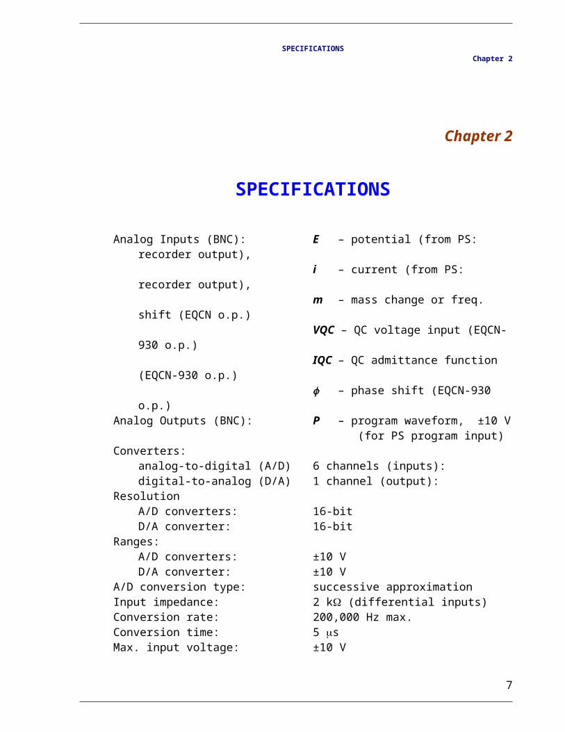
Analog Inputs (BNC): E – potential (from PS: recorder output),i – current (from PS: recorder output),m – mass change or freq. shift (EQCN o.p.)

VQC – QC voltage input (EQCN-930 o.p.)

IQC – QC admittance function (EQCN-930 o.p.)

– phase shift (EQCN-930 o.p.)Analog Outputs (BNC): P – program waveform, ±10 V

(for PS program input)Converters:

analog-to-digital (A/D) 6 channels (inputs):digital-to-analog (D/A) 1 channel (output):

ResolutionA/D converters: 16-bitD/A converter: 16-bit

Ranges:A/D converters: ±10 VD/A converter: ±10 V

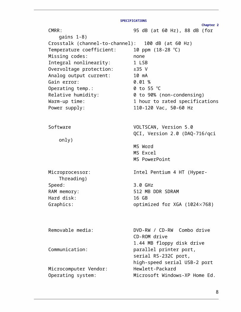
A/D conversion type: successive approximationInput impedance: 2 k (differential inputs)Conversion rate: 200,000 Hz max.Conversion time: 5 sMax. input voltage: ±10 V CMRR: 95 dB (at 60 Hz), 88 dB (for gains 1-8)Crosstalk (channel-to-channel): 100 dB (at 60 Hz)Temperature coefficient: 10 ppm (18-28 oC)Missing codes: noneIntegral nonlinearity: 1 LSBOvervoltage protection: ±35 VAnalog output current: 10 mAGain error: 0.01 %Operating temp.: 0 to 55 oCRelative humidity: 0 to 90% (non-condensing)Warm-up time: 1 hour to rated specificationsPower supply: 110-120 Vac, 50-60 Hz

4

SPECIFICATIONS Chapter 2

Software VOLTSCAN, Version 5.0QCI, Version 2.0 (DAQ-716/qci only)MS WordMS ExcelMS PowerPoint

Microprocessor: Intel Pentium 4 HT (Hyper-Threading)Speed: 3.0 GHzRAM memory: 512 MB DDR SDRAMHard disk: 16 GBGraphics: optimized for XGA (1024768)

Removable media: DVD-RW / CD-RW Combo driveCD-ROM drive1.44 MB floppy disk drive

Communication: parallel printer port,serial RS-232C port,high-speed serial USB-2 port

Microcomputer Vendor: Hewlett-PackardOperating system: Microsoft Windows-XP Home Ed.

5

INSTALLATION Chapter 3

Chapter 3

INSTALLATION

All software necessary to operate the Data Logger is factory installed and the instrument is ready to run. The information below is provided in case a software re-installation or up-grade is needed.

Software re-installation or upgrade

Turn the computer on and wait until Microsoft Windows-98/ME/2000/XP boots up. If you already have the computer turned on, exit from any program you might be in and close all other running programs. On the computer screen, you should have only a desktop and no working windows open. The quick launch panel (the one with Windows START button) should indicate that there are no running programs.

Press the button on the CD-ROM drive to open the drive door. Insert the Voltscan CD-ROM disk and close the door by slightly pushing the drive drawer. Wait a few seconds (it can be, sometimes, up to a minute) until the installation program recorded on the Voltscan CD is loaded and shows up on the screen. If, for any reason, the auto-run feature does not work and the auto-installation program does not start automatically, use the Windows Explorer and go to the CD-ROM drive. Find the INSTALL.exe program in the main directory and click on it to start the Voltscan installation manually.

The installation is self-explanatory and does not require any additional comments. After the software installation has successfully been completed, open the CD-ROM drive, remove the disk, and store it in a safe place free of dust and moisture. Restart the computer.

6


File structureThe following information may help you in further

configuring your data file structure.The executable program files and binary files necessary for

operation of the main program are stored in c:\Program Files\Elchema\Voltscan 5.0 and other c:\Program Files\Elchema folders. Do not open or change any of the files included in these folders as the program may not then run correctly or may not run at all. However, you can access the information stored in the folder c:\Program Files\Elchema\Manuals, which contains manuals for a potentiostat, quartz crystal nanobalance, Voltscan software, tips for setting up your experimental system, etc.

The user data files can be stored in any folder (directory). The default folder is:

c:\data5

which contains example .vv5 data files.You can create additional folders with names reflecting different series of experiments, e.g.:

c:\data\copperc:\data\silverc:\data\PPyetc.

or:My Documents\data5\copperMy Documents\data5\silverMy Documents\data\PPyetc.

If you are going to collect large amounts of files, you may consider storing some data on recordable compact disks CD-R's, removable floppy diskettes, IOmega ZIP-disks, Compact Flash cards, tapes, or other media. You can transfer some folders with data files to the removable media later on for the purpose of proper storage or to make some more space in the computer. Consider also saving copies of important data files on external media as a backup to prevent any accidental data loss.

The installation program creates also some icons, which are painted onto the desktop. These are short-cuts to Voltscan data acquisition program and to the data directory. They will help you to start quickly the acquisition experiments and view data files.

7


After the installation has been completed, you can run VOLTSCAN (refer to the next Chapter). Voltscan based Data Loggers DAQ-716v have D/A and A/D converters assembled and tested and do not require any further attention.

8

HOW TO START VOLTSCAN PROGRAM Chapter 4

Chapter 4

HOW TO START VOLTSCANPROGRAM

The information contained in this chapter can also be found in the the Voltscan manual. In case the software has been upgraded, follow the software manual, which brings the details of the Voltscan operation.

Initial conditions

If your computer is not on yet, turn on the computer and wait until Microsoft Windows-98/ME/2000/XP boots up. If you are already working on the computer, exit from any program you are in. It is recommended to close all other running programs as they may interfere with the data logger timing functions. On the computer screen, you should have only a desktop and no working windows open.

The ways to start

You can start Voltscan 5.0 Data Acquisition and Control program or QCI 2.0 program in at least two ways:(1) On the desktop, find a corresponding icon, which is marked Voltscan 5.0 or QCI 2.0 and double-click on it. It will start the program automatically. (2) Click the Windows START button located on the Quick Launch bar at the bottom or at the side of the screen. Select PROGRAMS option, and then ELCHEMA group, and VOLTSCAN or QCI software. Click on it to start it to start the program.

9

HOW TO START VOLTSCAN PROGRAM Chapter 4

Startup procedure

Right after the Voltscan program has been started, it displays a bitmap picture with program name VOLTSCAN, Version 5.0. When asked for a password, type it in and press the ENTER key. For Data Logger computers set up in the Elchema factory, the principal investigator name is usually entered as the password, which is then remembered by the computer, and you need only to press the CONFIRM button. The program initialization routines load standard parameter sets from disk and then load the last data recorded in the previous session with Voltscan. These experimental data are stored in the file LastData.vv in the folder c:\Program FIles\Elchema\Voltscan. These data are automatically scaled and plotted on the screen canvas. To prepare experimental parameters for a new experiment, click on the PARAMS button located on a Cool Bar in the upper part of the screen. This will activate the Tabbed Notebook with parameters to set. Follow the instructions to modify the program waveform, plot scaling, etc., described in the next chapters.

10

PROGRAM WAVEFORM Chapter 5

Chapter 5

PROGRAM WAVEFORM

To set parameters of the analog program waveform, which controls the potentiostat, enter the Tabbed Notebook by clicking on the PARAMS button located on the Cool Bar in the upper part of the screen. Select the page of the notebook named WAVE by clicking the tab with that label. Alternatively, you can select Waveform in the main menu, which will activate Notebook, if it is not active, and open the page Wave.

Types of waveform parameters

The program waveform parameters to set up include two types of parameters:(1) the waveform shape characteristic and (2) parameters of the digitizing process.

In order to define the waveform shape, you have to specify the waveform vertexes, scan rates, holding times, and number of semi-cycles. The digitizing specification will include the number of points to be collected and the number of measurements to be done for averaging of each data point collected.

Waveform shape

The waveform is composed of segments, which include holding at a constant potential and scans or steps. A combination of holding and scan, or holding and step, is called a stage (or semi-cycle). In the wave parameters table, four sets of values including the limit potential En, holding time n, and scan rate sn, are presented. Here, the potential E1 is the initial potential and the holding time 1 corresponds to the holding at the initial potential. The value s1 indicates the potential scan

11


rate, in mV/s, for a scan from potential E1 to potential E2. The potential E4 is the final potential. By definition, the scan rate of 0 is interpreted as a step. In other words, '0' replaces infinitely high scan rate (corresponding to a step). From now on, by scanning we will mean a potential scan or step. The number of stages can be set from 0 to 9 in the spin box labeled STAGES. If the total number of stages is 3, then the wave corresponds exactly to the three stages listed in the table, the final scan ending up at E4. If number of stages is greater than 3, then the stage 4 continues to potential E2, with holding there for 2 and scanning at rate s2 to the next potential (E3 or, if this is the final scan, to E4). The scanning between E2 and E3 continues until the last scan, which always ends up at E4. If the number of stages is less than 3, e.g. 2, then the second stage includes holding at E2 for 2 and scanning at a rate s2 to the final potential E4, omitting entirely stage 3. If the total number of stages is 1, then the first stage is composed of holding at E1 for 1 and scanning at a rate s1 to the final potential E4, omitting entirely stages 2 and 3.

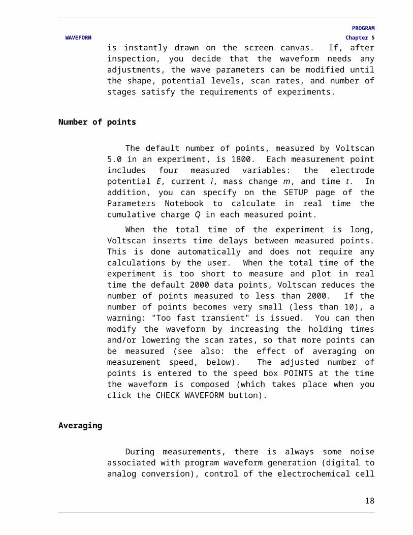
Although, the program waveform composing looks at first very complicated, after a few trials you will find it very quick and convenient. To see the immediate effect of the waveform settings, you can click on the button CHECK WAVEFORM. A graph of E vs. t is instantly drawn on the screen canvas. If, after inspection, you decide that the waveform needs any adjustments, the wave parameters can be modified until the shape, potential levels, scan rates, and number of stages satisfy the requirements of experiments.

Number of points

The default number of points, measured by Voltscan 5.0 in an experiment, is 1800. Each measurement point includes four measured variables: the electrode potential E, current i, mass change m, and time t. In addition, you can specify on the SETUP page of the Parameters Notebook to calculate in real time the cumulative charge Q in each measured point.

When the total time of the experiment is long, Voltscan inserts time delays between measured points. This is done automatically and does not require any calculations by the user. When the total time of the experiment is too short to measure and plot in real time the default 2000 data points, Voltscan reduces the number of points measured to less than 2000. If the number of points becomes very small (less than 10), a warning: "Too fast transient" is issued. You can then modify the waveform by increasing the holding times and/or lowering the scan rates,

12


so that more points can be measured (see also: the effect of averaging on measurement speed, below). The adjusted number of points is entered to the speed box POINTS at the time the waveform is composed (which takes place when you click the CHECK WAVEFORM button).

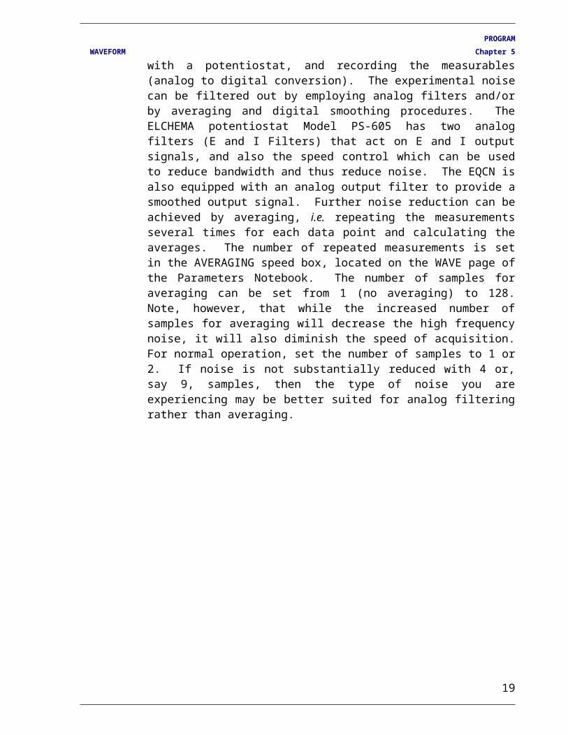
Averaging

During measurements, there is always some noise associated with program waveform generation (digital to analog conversion), control of the electrochemical cell with a potentiostat, and recording the measurables (analog to digital conversion). The experimental noise can be filtered out by employing analog filters and/or by averaging and digital smoothing procedures. The ELCHEMA potentiostat Model PS-605 has two analog filters (E and I Filters) that act on E and I output signals, and also the speed control which can be used to reduce bandwidth and thus reduce noise. The EQCN is also equipped with an analog output filter to provide a smoothed output signal. Further noise reduction can be achieved by averaging, i.e. repeating the measurements several times for each data point and calculating the averages. The number of repeated measurements is set in the AVERAGING speed box, located on the WAVE page of the Parameters Notebook. The number of samples for averaging can be set from 1 (no averaging) to 128. Note, however, that while the increased number of samples for averaging will decrease the high frequency noise, it will also diminish the speed of acquisition. For normal operation, set the number of samples to 1 or 2. If noise is not substantially reduced with 4 or, say 9, samples, then the type of noise you are experiencing may be better suited for analog filtering rather than averaging.

13

PLOT SCALE Chapter 6

Chapter 6

PLOT SCALE

Variables

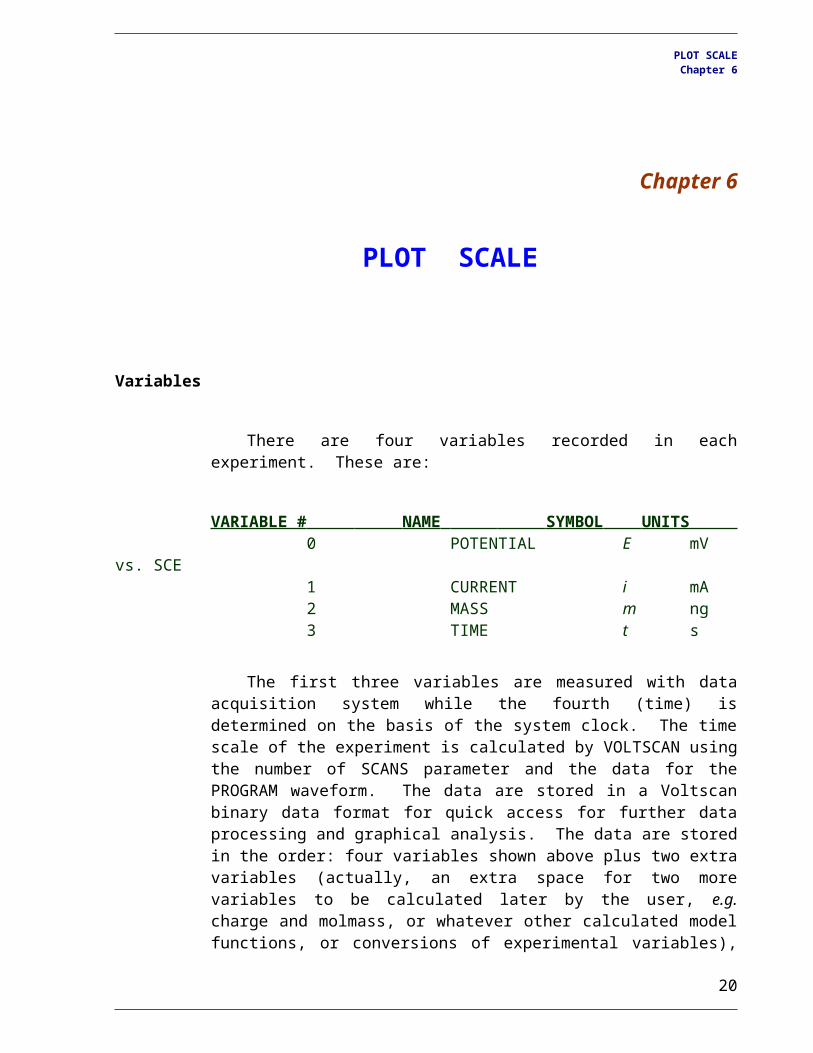
There are four variables recorded in each experiment. These are:

VARIABLE # NAME SYMBOL UNITS 0 POTENTIAL E mV vs. SCE 1 CURRENT i mA 2 MASS m ng 3 TIME t s

The first three variables are measured with data acquisition system while the fourth (time) is determined on the basis of the system clock. The time scale of the experiment is calculated by VOLTSCAN using the number of SCANS parameter and the data for the PROGRAM waveform. The data are stored in a Voltscan binary data format for quick access for further data processing and graphical analysis. The data are stored in the order: four variables shown above plus two extra variables (actually, an extra space for two more variables to be calculated later by the user, e.g. charge and molmass, or whatever other calculated model functions, or conversions of experimental variables), all for the first "data point", then all six variables values for the second "data point", and so on. The data are preceded and followed by a list of variable names, symbols, and units, number of points collected, etc. You do not need to know any details of the data format, or how many points have been collected. It is all transparent to the user. Just keep track of the file names and experimental conditions.

14


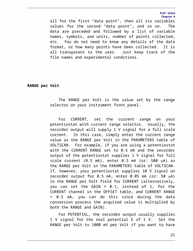
RANGE per Volt

The RANGE per Volt is the value set by the range selector on your instrument front panel.

For CURRENT, set the current range on your potentiostat with current range selector. Usually, the recorder output will supply 1 V signal for a full scale current. In this case, simply enter the current range value as the RANGE per Volt in the PARAMETERS table of VOLTSCAN. For example, if you are using a potentiostat with the CURRENT RANGE set to 0.5 mA and the recorder output of the potentiostat supplies 1 V signal for full scale current (0.5 mA), enter 0.5 mA (or: 500 A) as the RANGE per Volt in the PARAMETERS table of VOLTSCAN. If, however, your potentiostat supplies 10 V signal on recorder output for 0.5 mA, enter 0.05 mA (or: 50 A) in the RANGE per Volt field for CURRENT (alternatively, you can set the GAIN = 0.1, instead of 1, for the CURRENT channel in the OFFSET table, and CURRENT RANGE = 0.5 mA; you can do this since during the data conversion process the acquired value is multiplied by both the RANGE and GAIN).

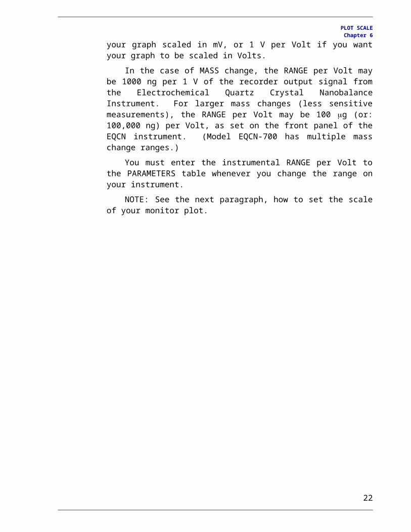
For POTENTIAL, the recorder output usually supplies 1 V signal for the real potential E of 1 V. Set the RANGE per Volt to 1000 mV per Volt if you want to have your graph scaled in mV, or 1 V per Volt if you want your graph to be scaled in Volts.

In the case of MASS change, the RANGE per Volt may be 1000 ng per 1 V of the recorder output signal from the Electrochemical Quartz Crystal Nanobalance Instrument. For larger mass changes (less sensitive measurements), the RANGE per Volt may be 100 g (or: 100,000 ng) per Volt, as set on the front panel of the EQCN instrument. (Model EQCN-700 has multiple mass change ranges.)

You must enter the instrumental RANGE per Volt to the PARAMETERS table whenever you change the range on your instrument.

NOTE: See the next paragraph, how to set the scale of your monitor plot.

15


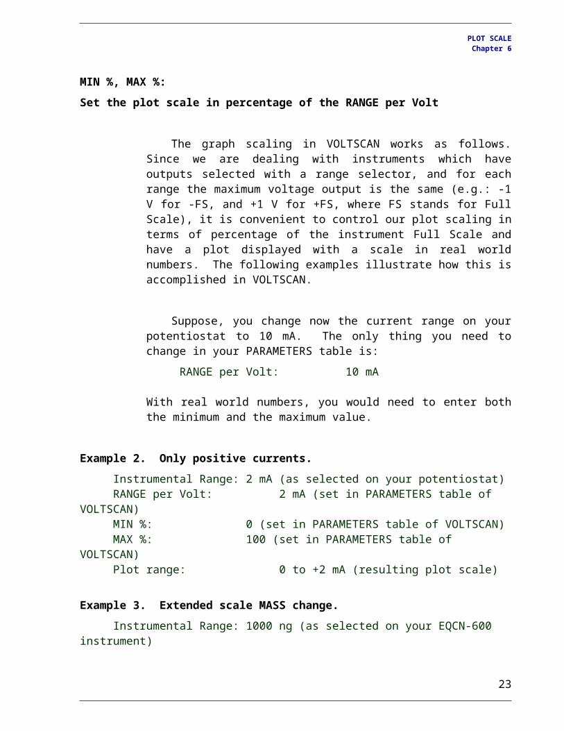
MIN %, MAX %: Set the plot scale in percentage of the RANGE per Volt

The graph scaling in VOLTSCAN works as follows. Since we are dealing with instruments which have outputs selected with a range selector, and for each range the maximum voltage output is the same (e.g.: -1 V for -FS, and +1 V for +FS, where FS stands for Full Scale), it is convenient to control our plot scaling in terms of percentage of the instrument Full Scale and have a plot displayed with a scale in real world numbers. The following examples illustrate how this is accomplished in VOLTSCAN.

Suppose, you change now the current range on your potentiostat to 10 mA. The only thing you need to change in your PARAMETERS table is:

RANGE per Volt: 10 mA

With real world numbers, you would need to enter both the minimum and the maximum value.

Example 2. Only positive currents.Instrumental Range: 2 mA (as selected on your potentiostat)RANGE per Volt: 2 mA (set in PARAMETERS table of VOLTSCAN)MIN %: 0 (set in PARAMETERS table of VOLTSCAN)MAX %: 100 (set in PARAMETERS table of VOLTSCAN)Plot range: 0 to +2 mA (resulting plot scale)

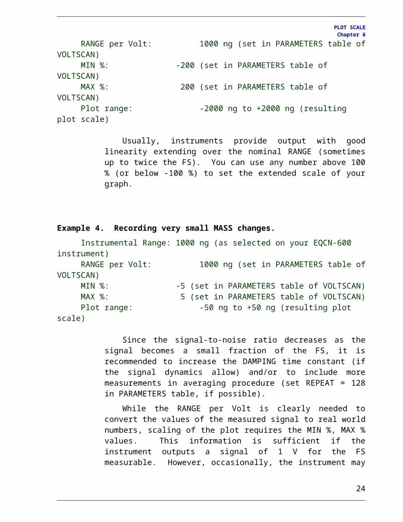
Example 3. Extended scale MASS change.Instrumental Range: 1000 ng (as selected on your EQCN-600 instrument)RANGE per Volt: 1000 ng (set in PARAMETERS table of VOLTSCAN)MIN %: -200 (set in PARAMETERS table of VOLTSCAN)MAX %: 200 (set in PARAMETERS table of VOLTSCAN)Plot range: -2000 ng to +2000 ng (resulting plot scale)

Usually, instruments provide output with good linearity extending over the nominal RANGE (sometimes up to twice the FS). You can use any number above 100 % (or below -100 %) to set the extended scale of your graph.

16


Example 4. Recording very small MASS changes.Instrumental Range: 1000 ng (as selected on your EQCN-600 instrument)RANGE per Volt: 1000 ng (set in PARAMETERS table of VOLTSCAN)MIN %: -5 (set in PARAMETERS table of VOLTSCAN)MAX %: 5 (set in PARAMETERS table of VOLTSCAN)Plot range: -50 ng to +50 ng (resulting plot scale)

Since the signal-to-noise ratio decreases as the signal becomes a small fraction of the FS, it is recommended to increase the DAMPING time constant (if the signal dynamics allow) and/or to include more measurements in averaging procedure (set REPEAT = 128 in PARAMETERS table, if possible).

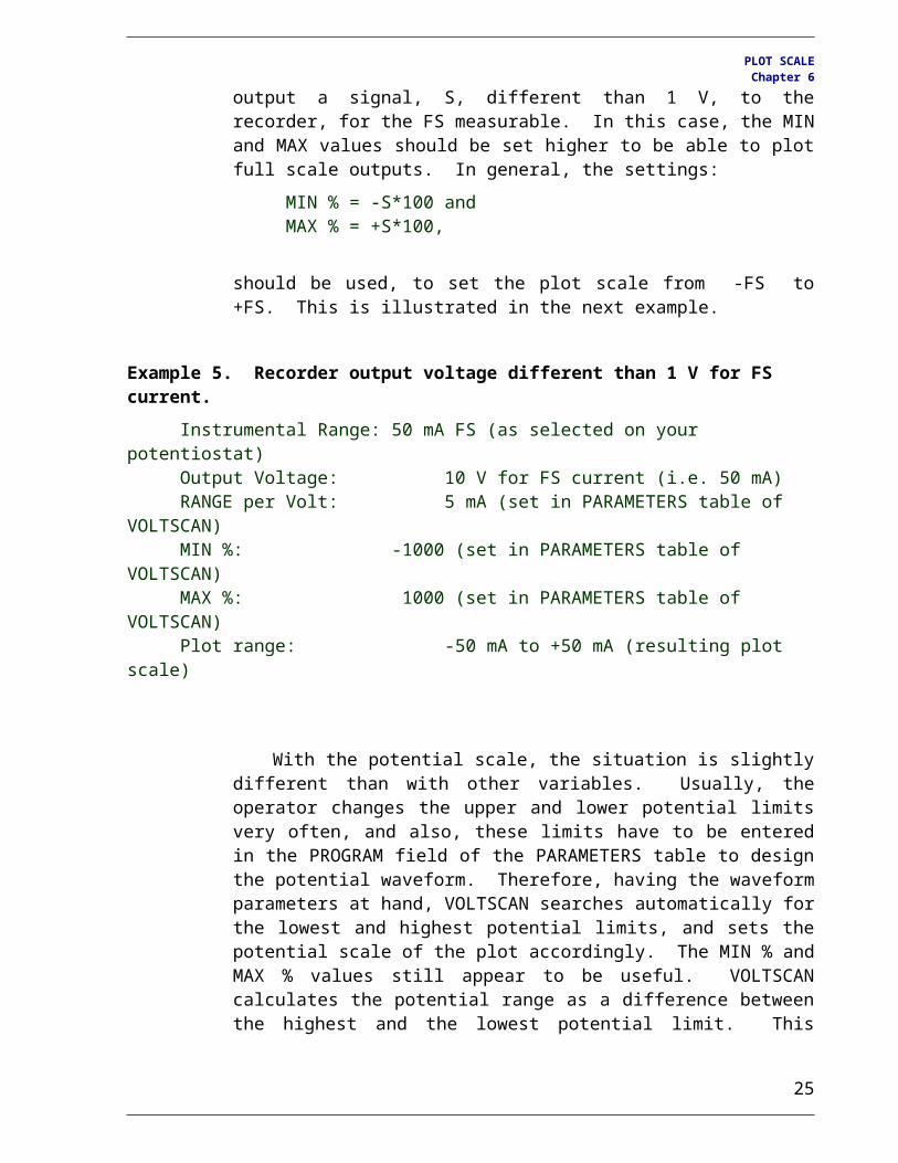
While the RANGE per Volt is clearly needed to convert the values of the measured signal to real world numbers, scaling of the plot requires the MIN %, MAX % values. This information is sufficient if the instrument outputs a signal of 1 V for the FS measurable. However, occasionally, the instrument may output a signal, S, different than 1 V, to the recorder, for the FS measurable. In this case, the MIN and MAX values should be set higher to be able to plot full scale outputs. In general, the settings:

MIN % = -S*100 andMAX % = +S*100,

should be used, to set the plot scale from -FS to +FS. This is illustrated in the next example.

Example 5. Recorder output voltage different than 1 V for FS current.Instrumental Range: 50 mA FS (as selected on your potentiostat)Output Voltage: 10 V for FS current (i.e. 50 mA)RANGE per Volt: 5 mA (set in PARAMETERS table of VOLTSCAN)MIN %: -1000 (set in PARAMETERS table of VOLTSCAN)MAX %: 1000 (set in PARAMETERS table of VOLTSCAN)Plot range: -50 mA to +50 mA (resulting plot scale)

With the potential scale, the situation is slightly different than with other variables. Usually, the operator changes the upper and lower potential limits very often, and also, these limits have to be entered in the PROGRAM field of the PARAMETERS table to design the potential waveform. Therefore, having the waveform parameters at hand, VOLTSCAN searches automatically for the lowest and highest potential limits, and sets

17


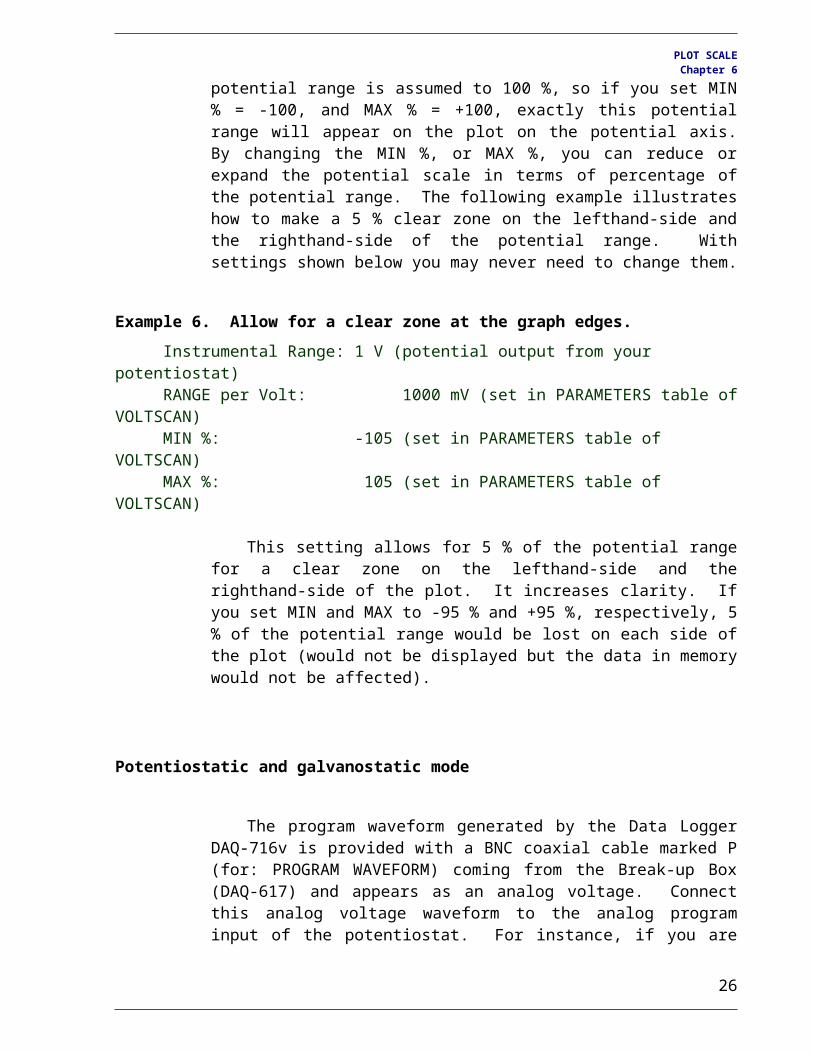
the potential scale of the plot accordingly. The MIN % and MAX % values still appear to be useful. VOLTSCAN calculates the potential range as a difference between the highest and the lowest potential limit. This potential range is assumed to 100 %, so if you set MIN % = -100, and MAX % = +100, exactly this potential range will appear on the plot on the potential axis. By changing the MIN %, or MAX %, you can reduce or expand the potential scale in terms of percentage of the potential range. The following example illustrates how to make a 5 % clear zone on the lefthand-side and the righthand-side of the potential range. With settings shown below you may never need to change them.

Example 6. Allow for a clear zone at the graph edges.Instrumental Range: 1 V (potential output from your potentiostat)RANGE per Volt: 1000 mV (set in PARAMETERS table of VOLTSCAN)MIN %: -105 (set in PARAMETERS table of VOLTSCAN)MAX %: 105 (set in PARAMETERS table of VOLTSCAN)

This setting allows for 5 % of the potential range for a clear zone on the lefthand-side and the righthand-side of the plot. It increases clarity. If you set MIN and MAX to -95 % and +95 %, respectively, 5 % of the potential range would be lost on each side of the plot (would not be displayed but the data in memory would not be affected).

Potentiostatic and galvanostatic mode

The program waveform generated by the Data Logger DAQ-716v is provided with a BNC coaxial cable marked P (for: PROGRAM WAVEFORM) coming from the Break-up Box (DAQ-617) and appears as an analog voltage. Connect this analog voltage waveform to the analog program input of the potentiostat. For instance, if you are using ELCHEMA Precision Potentiostat/Galvanostat, Model PS-605, the input C is the analog program input.

If you want to perform a potentiostatic experiment, select the option PS with the MODE switch on the potentiostat and choose PS in the MODE radio button section on the WAVE page of the Parameters Notebook in Voltscan. The voltage program waveform will be translated to the potential values of the same sign and magnitude (by 'potential' we mean the potential of the

18


working electrode vs. the reference electrode). Note that potentiostats from other vendors may have a program input with an inverted sign (i.e., corresponding to the potential of the reference electrode vs. working electrode).

If you want to perform a galvanostatic experiment, select the option GS with the MODE switch on the potentiostat and choose GS in the MODE radio button section on the WAVE page of the Parameters Notebook in Voltscan. The voltage program waveform will be translated to the current values. The program voltage of 1000 mV will generate current equal to the nominal current range selected on the potentiostat. For instance, if a current range 100 μA is selected on the potentiostat, the program voltage of -500 mV will generate current of -50 μA (i.e., 100*(-500)/1000 = -50 ). Negative program voltage generates a cathodic current, and positive program voltage generates an anodic current. Note that potentiostats of other vendors may have a different translation coefficient and even a different sign convention.

19

VARIABLES Chapter 7

Chapter 7

VARIABLES

The selection of variables to be plotted, both during an experiment as well as during a post-experiment inspection, is done by means of the variables table and pull-down boxes available on the page VARIABLES in the Parameters Notebook. With the pull-down boxes, which list all variable symbols currently used by the system, you can select variables for two ordinates (left and right) and for abscissa. If only one ordinate is desired, select NONE for the variable for second ordinate.

DAQ channels: variables to be measured

The three variables recorded in each experiment are digitized using channels 0, 1, and 2 of the Data Logger, as follows:

CHANNEL # VARIABLE SYMBOL 0 POTENTIAL E 1 CURRENT i 2 MASS m

The fourth variable (time t) is determined on the basis of the system clock. The time scale of the experiment is calculated by VOLTSCAN using the number of STAGES parameter and the data for the PROGRAM waveform. The data are stored in the Voltscan binary data format for quick access for further data processing and graphical analysis. The data are stored in the order: four variables shown above plus two extra variables (i.e., an extra space for two more variables to be calculated later by the user, e.g. charge and molmass, or whatever other calculated model functions, or conversions of experimental variables), all for the first 'data point', then all six variables values for the second 'data point', and so on. The data are preceded and followed by a list of

20

VARIABLES Chapter 7

variable names, symbols, and units, number of points collected, etc. You do not need to know any details of the data format, or how many points have been collected. It is all transparent to the user. Just keep track of the file names and experimental conditions. You can load this set of variables by clicking on the LOAD DEFAULT VARIABLES button located on the VARIABLES page of the Parameters Notebook.

Changing units

If it is necessary to change the units of any variables, it can be done by simply replacing the old units with new ones. To do that, click on the appropriate cell of the VARIABLES table to gain focus on that cell and type in the new units. The new units will appear on any graph drawn during the real-time data acquisition or when reviewing the data from finished experiment or from disk.

Adding and modifying variable names and symbols

In the same way, as for the units, described above, you can add or change variable names and symbols for the additional variables (#4 and #5). Do not attempt to change the first four variables, since they are assigned to the DAQ channels (and time, which is a system variable), as described earlier in this chapter, and cannot be modified. After any addition or change, click on the CONFIRM button to accept changes and transfer the new data into the pull-down boxes for Y1, Y2, and X axes.

You can save a frequently used set of variables and units by clicking on the button SAVE VARIABLES. This set of variables can readily be retrieved later on by clicking on the button LOAD VARIABLES. This set of variables will be automatically stored on a hard disk and, thus, can be retrieved in subsequent sessions with Voltscan.

21

RUNNING AN EXPERIMENT Chapter 8

Chapter 8

RUNNING AN EXPERIMENT

Set the program and other parameters first

Before you start an experiment, make sure you set all the parameters in the program waveform table and spin boxes on the WAVE page of the Parameters Notebook. Also, the plot scale should be set on the SCALE page of the Notebook. Finally, the variables to be plotted and their units should be set on page VARIABLES of the Notebook. It is recommended to always check the shape and levels of the waveform designed for the experiment. It is not time consuming but you can be sure that no mistakes are made with the program. If you perform a series of experiments with the same parameters, you do not need to invoke the Parameters Notebook and set the parameters again. Just save the data and click on the RE-RUN button to repeat the experiment. The program waveform is automatically loaded and read when you start the experiment.

Start experiment with the RUN button

To start an experiment, click on the WAVE/CHECK WAVEFORM/RUN buttons. The RUN button is located on the RUN the Run Panel displayed after pressing the CHECK WAVEFORM button. The CHECK WAVEFORM button starts the preparation routines for data acquisition and composes the waveform for potentiostat. A plot with the program waveform is then displayed on the screen canvas and the Notebook is deactivated. Another panel, the Run Panel, appears on the right-side of the screen with a RUN button and you can click on it to start the experiment.

22

RUNNING AN EXPERIMENT Chapter 8

Make sure that your potentiostat and nanobalance, if any, are properly connected to the data logger and the program waveform is supplied to the potentiostat analog input. Before starting the program sequence execution, the CELL toggle switch in potentiostat should switched to ON and the program input switch to ON.

The parameters from the Parameters Notebook are used to initialize the data acquisition board. A prescaled plot is displayed on the screen at the beginning of an experiment, after you click on the RUN button. Since the initialization of the DAQ board takes ca. 1-2 seconds, the data do not show up on the graph immediately, but only after this initialization period. The initialization is performed at the beginning of each experiment.

During the acquisition, a message "Acquisition in progress" is displayed on the screen, on a Cool Bar. Do not interrupt the acquisition process. When the experiment is finished, another message is displayed: "Acquisition finished". At that time, you can inspect the data collected, replot them, autoscale, change variables, etc. But, most importantly, you must save the data on a hard disk or removable media before a new data set takes its place in the computer RAM memory.

If you are going to use the same set of data acquisition parameters for the next experiment, as in the preceding experiment, you do not need to invoke the Parameters Notebook again before clicking on the RE-RUN button. The program waveform and other parameters are stored in computer memory and read automatically when you start new experiment.

23

SAVE AND LOAD OPERATIONS Chapter 9

Chapter 9

SAVE AND LOAD OPERATIONS

The save and load operations in Voltscan conform to the Microsoft Windows-98/ME/2000/XP standards and do not require any detailed descriptions. However, it is important to introduce the user to the special formats the experimental data can be stored in for further processing. These include two file formats:(1) binary format,(2) ASCII (or: text) data format.

The basic data format is the Voltscan 5 binary data format. The binary files store the measured data, variable specifications, and all the experimental conditions. Retrieving a binary files is, therefore, equivalent to loading the corresponding experimental conditions, which may be useful for future reference. The binary files are also more compact and are saved and loaded faster than text files.

The Voltscan 5.0 ASCII data files contain the information about the number of variables (by default: 6) and the number of data points. This information is followed by the specification of variables and their units. The following measured data are organized in this way: first, the values for each of the six variables corresponding to the first experimental point are listed and separated by the tab characters; then the values for each variable corresponding to the second experimental point are listed, followed by those for the third point, and so on. The data for each point are separated by the line feed and carriage return character. The ASCII data files are larger and so they occupy more of the disk storage space. Also, the saving of these files is slower.

While the normal operation of Voltscan 5, and also earlier versions, is based on the binary data format, at the stage of data processing, the ASCII format is useful, since it allows the user to utilize plotting and processing capabilities of software packages

24

SAVE AND LOAD OPERATIONS Chapter 9

available from other vendor, e.g. Microsoft EXCEL, Microcal ORIGIN, etc.

NOTE: Voltscan 5 is not compatible with earlier versions of Voltscan (1-4), which used a different file structure. The earlier binary format was based on 32-bit (6-byte) real numbers and reduced specification of experimental conditions. The Voltscan 5 binary file format is now based on double-precision 64-bit (8-byte) real numbers. However, Voltscan 5 program can recognize the old file format and load data from these files without operator intervention. The file name extension, both in the old files and the new files, are not essential. This means that you can add an extension .vv5 to the Voltscan files but the file can be retrieved with any other extension too, e.g., .123, .dat, etc. This is not the case, however, with the ASCII files, since Microsoft's EXCEL will not be able to import data from a text file, which has an extension different than .txt. Therefore, when saving a file in an ASCII format, do not force Voltscan to make a different extension than the default .txt extension, which is added automatically by Voltscan.

The data collected during an experiment are stored in the computer RAM (volatile) memory. If you are satisfied with the experiment, the data should be saved on disk.

You can save data after experiment by using one of the two possible routes:(a) by clicking on one of the SAVE AS buttons on the Cool Bar (one button is for saving data in a binary format and one for saving data in an ASCII format), or(b) by a proper selection in the main menu:

Alt/File/Save as Binary, or Alt/File/Save as ASCII.

25

DATA PROCESSING AND GRAPHICS Chapter 10

Chapter 10

DATA PROCESSING AND GRAPHICS

A variety of data processing and graphic control functions can be found in the main menu utilities: PLOT, DATA, TOOLS, and CALC. Most of these utilities are self-explanatory and base on the common MS Windows customs and procedures. A brief description of these functions follows:

PLOTThe PLOT group includes controls for manual scaling and autoscaling, specifications for curve drawing, such as the line, dots, marks, etc.; their color, and line thickness. Note that thicker lines may need to be selected for the purpose of printing and thinner for display on the monitor. The standard color setting for variables is the default setting but you can change it to any other color available on the palette.

DATAMost of the data processing functions are in this group. The meaning of the functions is as follows:CLEAR DATA deletes all data from Data Logger memory,DRAW ORIGINAL redraws original experimental data if they are

still present in memory,SMOOTH Savitzky-Golay 7-point digital data smoothing,LINEFIT least-squares linear fitting to a data range

selected with a cursor. Note that the two limiting points you select on the curve to define the data range do not need to be exactly on the curve since Voltscan will search the neighborhood to find the closest line and point on it. Once two points are selected, the line

26


statistics panel will appear with values of the slope, intercept, and correlation coefficient.

INTEGRATE Q=$idt Voltscan searches for variables: i and t, performs integration point-by-point, stores the calculated charge in variable Q, and then automatically scales and displays the Q function vs. the current x-axis variable.

INTEGRATE f=$ydx Similar to the integration Q=$idt, but in this case Voltscan uses y and x variables from the current graph (left and bottom axes) and performs the integration.

DIFFERENTIATE A differentiation dy/dx (y and x being the left and bottom axis variables, respectively) is performed. Note that a very smooth data are needed for this function to work well since differentiation amplifies even very little noise if present on an experimental curve.

PEAK PARAMS Creates a square-box cursor and searches for extremum on the curve. The peak data are automatically written to the Log-Book. Press the LOG-BOOK button to open the Log-Book. Press ESCAPE or AUTOSCALE to end PEAK search session.

POINT COORDINATES Data cursor that finds and displays coordinates on the Coordinate Panel.

RANGE SELECT Allows to select a range of points on a curve. That range can then be redrawn in an enlarged format (zoom) for further processing.

SECTION AVERAGE Selects a range of points and performs statistics on them with main goal to determine the mean value.

DISTANCE VERTICAL Allows one to select two points on a given curve (e.g. i in CV) and finds vertical distance between them.

MASS OFFSET Shifts all MASS data points by the value of the first measured point. In this way the MASS curve is offset to start at m = 0.

27


TOOLSThe following functions can be found in the TOOLS utilities:CHANGE PASSWORD - self-explanatory,FREE CURSOR While the data cursors operate basically on

curves (on data points), the free cursor can be used to read coordinates at any point on the graph.

DRAW FREE LINE A free line unconnected to any data points can be drawn on a graph for further analysis.

DRAW ARROW Very useful for marking graphs such as the m-E in which the direction of mass changes is not always very clear and must be explicitly shown with arrows.

DELETE LINES Deletes all lines including linefits, horizontal and vertical sections, arrows, and free lines from the graph and from the computer memory.

CALCThe CALC utility is located on the VARIABLES page of the Tabbed Notebook. It allows to graph a range of functions of variables using a simple three-step operation:(1) select variable to be converted by clicking on it in the variable list table,(2) if the function you are going to apply uses any constants, enter the constants values in edit boxes provided,(3) select the function from a list and click on it. The function is automatically calculated for all data points, scaled, and displayed on the graph.

28

ENDING THE SESSION WITH VOLTSCAN Chapter 11

Chapter 11

ENDING THE SESSION WITH VOLTSCAN

Be sure that your data set present in the volatile computer RAM memory is saved on hard disk or removable storage media, such as the floppy diskette, CD-RW optical disk, ZIP disk, solid state flash memory card, etc. To leave the program, it is essential to follow the exit procedure. It is important because various operating parameters must be saved and all open files closed before the program is terminated. Otherwise, some system data may be lost and the program may not work properly next time the computer is turned on.

The exit procedure includes activation of the Parameters Notebook (click on the PARAMS button, if it is not in an active state), selecting the EXIT page, and clicking on the QUIT button. Alternatively, you can go through the main menu and select:

Alt/File/Exit.

It is important to turn the CELL switch on your potentiostat OFF, before exiting from Voltscan program and turning off the Data Logger. The toggle switch for PROGRAM waveform input in potentiostat should also be turned OFF.

29