Data Gathering with Compressive Sensing in

Wireless Sensor Networks: An In-Network

Computation Perspective

Haifeng Zheng, Xinbing Wang, Xiaohua Tian, Shilin Xiao

Dept. of Electronic Engineering, Shanghai Jiao Tong University, P.R.China

Emails: zhenghf, xwang8, xtian, slxiao@sjtu.edu.cn

Abstract

In this paper, we investigate the fundamental performance limits of data gathering with compressive

sensing (CS) in wireless sensor networks, in terms of both energy and latency. We consider two scenarios

in which n nodes deliver data in centralized and distributed fashions, respectively. We take a new

look at the problem of data gathering with compressive sensing from the perspective of in-network

computation and formulate it as distributed function computation. We propose tree-based and gossip-

based computation protocols and characterize the scaling of energy and latency requirements for each

protocol. The analytical results of computation complexity show that the proposed CS-based protocols

are efficient for the centralized fashion. In particular, we show the proposed CS-based protocol can save

energy and reduce latency by a factor of Θ(√n lognm ) when m = O(

√n logn) in noiseless networks,

respectively, where m is the number of random projections for signal recovery. We also show that our

proposed protocol can save energy by a factor of Θ(√n

m√logn

) compared with the traditional transmission

approach when m = O(√

nlogn ) in noisy networks. For the distributed fashion, we show that the

proposed gossip-based protocol can improve upon the scheme using randomized gossip, which needs

fewer transmissions. Finally, simulations are also presented to demonstrate the effectiveness of our

proposed protocols.

Index Terms

In-network computation, data gathering, compressive sensing, wireless sensor networks.

Part of this paper is to appear in the Proceedings of IEEE INFOCOM 2012 (mini-conference) [31].

2

I. INTRODUCTION

Wireless sensor networks (WSNs) consisting of a large number of nodes, are usually deployed

in a large region for environmental monitoring, security and surveillance. Such networks are

typically designed to sense a field of interest, process sensed values, and transport data to one or

multiple sink(s). It is inefficient in many situations for directly transmitting all the raw data to

the sink(s). In particular, a sensing field usually exhibits high correlation between the measured

data and can be compressible in some transform domains. Thus, it is possible to deliver less

data to the destination without sacrificing the salient information. Therefore, it is desirable to

cooperate between the nodes and process the data in the networks so that the transport load can

be reduced. However, conventional aggregation techniques only capture some limited statistical

qualities, such as maximum, average of the measured data. Distributed source coding approaches,

such as Slepian-Wolf Coding [2], are also difficult to be applied in such scenarios since the prior

knowledge about the characteristics of data distribution should be known in advance.

Fortunately, compressive sensing (CS) provides an alternative approach for correlated data

transmission in an efficient manner. Compressive sensing allows for signal recovery with high

probability from a small number of random projections, i.e., random linear combinations of

measurements, as long as the signal is sparse or compressible in some domain [3]. In this paper,

we consider the application of compressive sensing in a data gathering scenario, where the

data collected by the sink is assumed to be spatially correlated [1]. In particular, we address the

following questions: how can we generate random projections from spatially distributed data, and

deliver them efficiently to the destination. What is the scaling of energy and latency requirements

to transmit these random projections over the network so that the original data can be recovered.

To answer these questions, we take a new look from the perspective of in-network computation.

We attempt to formulate the problem of data gathering with compressive sensing as distributed

function computation, and construct a multiround random linear function to compute random

projections. Such a function has much lower dimensions than the original signal, which reduces

the number of measurements that require to be transported in the network. In fact, the problem

we consider in this paper boils down to how to efficiently compute the given function and route

the computation results to the destination in the network. To address this problem, we study the

3

performance of routing and computing function in random geometric networks in terms of both

energy consumption and latency. To the best of our knowledge, this is the first work to analyze

the performance of energy consumption and latency for data gathering with compressive sensing

from the perspective of in-network computation.

The focus of this paper concentrates on devising efficient protocols for in-network function

computation in wireless sensor networks. We propose computation protocols for centralized and

distributed fashions, respectively. In the centralized fashion, we propose tree-based computation

protocols for both noiseless and noisy networks, where sensor nodes collect data , compute the

function and forward the results to the parents. The final computation results are obtained at the

destination which completes one round of in-network function computation. However, such a

protocol is susceptible to the failure of nodes and links. Specially, the failure of the destination

will cause the loss of all the computation results. In the distributed fashion, we propose a gossip-

based computation protocol, where the computation results can be available in each sensor node.

Thus, the gossip-based protocol provides a more robust approach to the failure of nodes and

links than the tree-based protocol. However, the robustness achieved in such a protocol is at the

cost of extra energy consumption. Our contributions are summarized as follows:

• For the first time, we formulate the problem of data gathering with compressive sensing as

in-network function computation. We construct a multiround random linear function, and

devise protocols for evaluating such a function computing in random networks.

• We propose tree-based computation protocols and analyze the scaling of computation com-

plexity in terms of energy consumption and latency for both noiseless and noisy networks.

We show that the computation protocols are efficient for both two networks. In particular,

the analytical results show that compared with the traditional transmission approach, the

proposed CS-based approach can save energy and reduce latency by a factor of Θ(√n lognm

)

when m = O(√n log n) in noiseless networks, respectively. We also show that our pro-

posed protocol can save energy by a factor of Θ(√n

m√logn

) compared with the traditional

transmission approach when m = O(√

nlogn

) in noisy networks.

• We propose a gossip-based computation protocol and derive the bounds of energy consump-

tion and latency based on the eigenstructure of the underlying graph in random networks.

4

We show that the gossip-based protocol can improve upon the scheme using randomized

gossip through theoretical analysis and simulations, which requires fewer transmissions.

Finally, simulation results are also presented to demonstrate the robustness of the gossip-

based protocol.

The remainder of this paper is organized as follows. In Section II, we review the related

work on in-network computation and data gathering with compressive sensing. In Section III,

we introduce the basic theory of compressive sensing, give the problem formulation and the

network model used in the paper. In Section IV, we propose a tree-based computation protocol

in noiseless random networks, and analyze the performance of computation in terms of energy

consumption and latency. In Section V, we present a tree-based computation protocol in noisy

random networks and study the scaling of energy consumption and latency of computation.

In Section VI, we also propose a gossip-based protocol for function computation, and derive

the bounds of energy consumption and latency. In Section VII, we carry out simulations to

demonstrate the performance of the proposed protocols. Finally, we conclude the paper in Section

VIII.

II. RELATED WORK AND DISCUSSION

In-network computation has been extensively studied in the past few years. Traditional dis-

tributed computation has been studied in terms of communication complexity in noiseless net-

works [11]. In [4], Giridhar and Kumar studied the computation of divisible functions and

symmetric functions over noiseless sensor networks. In [5], Khude and Kumar studied the scaling

laws for the time and energy consumption complexity of type-threshold functions computation

over random wireless sensor networks. Both these two work focus on noiseless networks.

Distributed computing in noisy networks was initially studied by El Gammal in [12], where

the communication complexity was studied in a noisy broadcast network model. The model

assums that when each node broadcasts one binary bit to its neighbors, the neighbors can

receive an independent noisy copy of the bit. Under this model, [12]–[15] studied computation

in noisy broadcast networks. Furthermore, [16]–[19], [32] studied computation in noisy random

geometric networks following the model of [12]. However, most of the above work concern

with computing certain functions with limited statistical qualities, such as max, mean, and sum

5

functions. Differently from most of previous work, we study the function computation which can

recover all source data from final computation results. More importantly, our work investigates

the performance of in-network computation in terms of energy consumption and latency, while

most of previous work concern only with energy consumption.

The above approaches to in-network computation are based on tree-based protocols, where

a forming spanning tree is rooted at the sink and then the computation results are aggregated

up to the tree. However, there are many drawbacks to these approaches. Firstly, the network

should provide undesirable information to establish and maintain routes, which results in energy

consumption overhead. Furthermore, unreliable links in wireless sensor networks may cause

the loss of all computation results since the computation results are only available at the sink.

To address the above problems, gossip algorithms have been proposed to solve the average

consensus problem. Several gossip algorithms have been proposed in [26]–[29], but again only

for some limited functions. A scheme using randomized gossip with compressive sensing has

been presented for a field estimation application in [6], [7]. However, we propose a gossip-based

protocol from the perspective of in-network computation in this paper. Moreover, we consider

transmission scheduling for the proposed computation protocol, which is a key issue we focus

on in our work.

On the other hand, the applications of compressive sensing for data gathering have been

studied in a few papers [20]–[23]. In [20], Luo et al. applied compressive sensing theory for

efficient data gathering in a large scale wireless sensor network. They showed that the proposed

scheme can substantially save communication cost and increase network capacity. In [21], Quer

et al. studied the behavior of CS in conjunction network topology and routing to transmit random

projections of the sensor data in a data gathering WSN. In [22], [23], Lee et al. investigated CS

for energy efficient data gathering in a multi-hop wireless sensor network. However, our work

studies data gathering with compressive sensing from the perspective of function computation

and characterizes the scaling laws of both energy consumption and latency in random networks.

6

III. PRELIMINARIES AND PROBLEM FORMULATION

A. Compressive Sensing Basics

Consider n sensor nodes deployed in a large-scale network measure temperature field. Let an

n× 1 column signal vector x = (x1, · · · , xn)T denote the signal obtained by the sensors in the

network. Suppose that in some n× n orthogonal basis Ψ = (ψ1, · · · , ψn)T , the signal x can be

represented as

x = Ψθ =n∑

i=1

θiψi, (1)

where θi is the coefficients of x in the basis Ψ. We reorder the coefficients θi in decreasing

magnitude such that

|θ1| ≥ |θ2| ≥ |θ3| ≥ · · · ≥ |θn|. (2)

If the ith largest transformation coefficient satisfies

|θi| ≤ Ri−1/p, R > 0, p ∈ (0, 1], (3)

we say that the signal x is a power-law decay signal in the basic Ψ. The best k-term approximation

of x is given by x =∑k

i=1 θiψi. We say that x is sparse or compressible in Ψ when the mean

squared approximation error behaves like

∥x − x∥2 ≤ Ck−1/p+1/2 (4)

for some constant C > 0, where the parameter p controls the compressibility of x in Ψ.

However, the coefficients θ are not easy to compute in WSN and the k most significant

coefficients are not usually known in advance. In order to avoid this problem, we make use of

the theory of compressive sensing. For the signal x, we can obtain the compression version y

through a measurement matrix Φ, i.e., y = Φx, where Φ is m×n random Gaussian or Bernoulli

matrix with m≪ n. Each element yi in the vector y is also called as random projection, which

can be computed as an inner product of form

yi =n∑

j=1

Φijxj. (5)

The theory of CS states that a k-sparse signal can be recovered from m random projections with

high probability if m ≥ ck log(n), where c is a small constant [9]. This indicates the number of

random projections m required for signal recovery scales linearly with signal sparsity k, and is

7

only logarithmic in signal length n. Recovering the signal x from y can be conducted through

solving an ℓ1-minimization problem:

minθ∈ℜN

∥ θ ∥ℓ1 s.t. y = ΦΨθ, x = Ψθ. (6)

If the signal x contains noise, recovery can be achieved by solving the following relaxed ℓ1-

minimization problem:

minθ∈ℜN

∥ θ ∥ℓ1 s.t. ∥ y − ΦΨθ ∥ℓ2< ε, x = Ψθ, (7)

where ε is a predefined error threshold.

B. Problem Formulation

Considering the scenario where the sink needs to collect data from n sensor nodes in the

network. At a sampling instant, sensor node j takes a measurement xj . Let x = (x1, · · · , xn)

denote the vector of measurements sampled by sensor nodes, where x is compressible. As stated

above, the processing of data gathering with compressive sensing consists of two parts: collecting

random projections y and recovering the signal x from y, which correspond to computing (5)

and solving (6) or (7), respectively. In fact, the former part can be viewed as the problem of

in-network function computation. The target function can be represented as a multiround random

linear function, which has the following form

F : xn → ym (8)

where y is the vector of random projections received by the sink, i.e., y = y1, · · · , ym and x

is the source vector generated by sensor nodes, i.e., x = x1, · · · , xn. The function Fi can be

written as∑n

j=1 Φijxj when the ith random projection yi is computed, where Φij are the entries

of a random Gaussian or Bernoulli matrix. When the function Fi is computed for m rounds,

the multiround random linear function computation is completed. In this paper, we focus on

devising protocols to efficiently perform computation of such a function in a random geometric

network. To measure the efficiency of a protocol, we consider energy consumption and latency

of a protocol, which are measured by the number of transmissions and the number of time

slots that the protocol takes to complete one round of the multiround random linear function

computation, respectively. We assume that each transmission consumes a fixed energy since the

each measurement has a constant length of the value.

8

C. Network Model

In this paper, we model the wireless sensor network as a random geometric graph G(V,E),

which consists of n nodes randomly deployed in a unit square. We assume all nodes share a

common wireless channel and the transmission range of the nodes is denoted by r(n). Let Xi

denote the location of sensor node i and |Xi −Xj| denote the Euclidean distance between node

i and node j. We adopt the protocol model [10], which is defined as follows:

Definition 1: Protocol Interference Model. When node i transmits to node j, the transmission

is successful if the following two conditions are satisfied

1) The distance |Xi − Xj| between node i and j is not greater than the transmission range

r(n), i.e., |Xi −Xj| ≤ r(n).

2) For other node k which transmits at the same time, the distance |Xk −Xj| between node

k and j should be greater than (1 +∆)r(n), i.e., |Xk −Xj| ≥ (1 +∆)r(n), where ∆ is a

positive constant that determines the size of the guard zone to prevent interference.

D. Cell Partition and Scheduling

Now we introduce our cell partition method adopted in our work. The unit square is tessellated

into cells with side length cn =√κ log n/n. We have the following lemma about network

connectivity.

Lemma 1: To guarantee connectivity with high probability, the following statements hold:

1) Each cell has Θ(log n) nodes with high probability when κ ≥ 8.

2) If the transmission range of a node is set to r(n) = 8√log n/n, each node in a cell can

communicate with any other node in the adjacent cells.

Proof: The proof of (1) follows easily from the result in [24]. The number of nodes ni in

any cell i satisfies

Pr(κ2log n ≤ ni ≤ 4κ log n∀i

)> 1− 2n(1−κ

8)

κ log n(9)

for large n. Thus, when κ ≥ 8, each cell has Θ(log n) nodes with high probability. For part (2),

we select κ = 8 and set the transmission range of a node r(n) = 2√2cn = 8

√log n/n which

is the maximum distance between two arbitrary nodes in adjacent cells so that a node in a cell

can communicate with any node in adjacent cells.

9

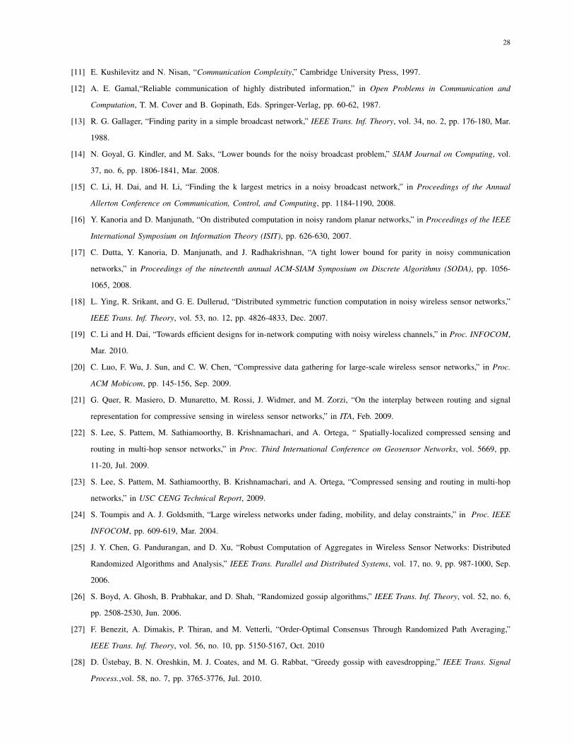
A K2-TDMA cell scheduling scheme is adopted in this paper. In this work, we use K2 colors

to schedule cells transmissions. Time is divided into slots and each slot is allocated to one cell

with the same color in different super cells, which is composed of K ×K cells. Fig.1 describes

an example of TDMA cell scheduling scheme with K = 3. The nodes in each cell take turns

to transmit to the nodes in the neighboring cell. Since cells with the same color in the adjacent

super cells are Kcn distance apart from each other, the minimum distance between a receiver

and other simultaneous transmitter should be set to (K − 2)cn ≥ (1 + ∆)2√2cn to guarantee

that concurrent transmissions can be successful without interfering with each other. Here, K is

a constant independent of n since K is only related to the value of ∆. Hence, the value K is

determined by the following lemma to guarantee that the nodes with the same color in super cells

can transmit simultaneously without interference. Using this scheduling scheme, the protocols

proposed in this paper can be oblivious in the sense that the transmission of a node is decided

in advance without causing collisions in any time slot. Such a cell scheduling scheme has been

commonly used in function computation [18], [19].

Lemma 2: If K ≥ 2 + (1 + ∆)2√2, there exists a TDMA scheme such that one node per

cell with the same color can simultaneously transmit a packet to all nodes in adjacent cells

successfully.

E. Preliminaries

In this subsection, we present a few results which are useful for our analysis in this paper.

Lemma 3: (Repetition Coding [33]): If a bit is sent M times over a binary symmetric channel

with error probability bounded above by a constant ϵ, then the probability of decoding error by

a majority rule is no greater than

(4ϵ(1− ϵ))12M . (10)

Lemma 4: [19]: For any γ > 0 and any integer m ≥ 1, there exists a codeword such that

an m-bit integer can be correctly received by a receiver with probability at least 1− e−γm with

O(m) broadcasts over a binary symmetric channel.

Lemma 5: (Khintchines inequality [30] ): Let b ∈ CM and ϵ = (ϵ1, . . . , ϵM) be a Rademacher

10

sequence. Then, for all p ≥ 2,(E|

M∑j=1

ϵjbj|p)1/p

≤ 23/(4p)e−1/2√p∥b∥2. (11)

IV. TREE-BASED COMPUTATION PROTOCOL WITH COMPRESSIVE SENSING IN NOISELESS

RANDOM NETWORKS

In this section, we first propose a tree-based protocol to compute the multiround random linear

function in noiseless random networks and then analyze the performance of the computation

protocol. Finally, we discuss the performance comparison with the traditional transmission

approach.

A. Protocol

As mentioned in Section III, since the unit square is divided into cells with side length

cn =√

8 log n/n, the total number of cells is l = ⌈√n/8 log n⌉2. By Lemma 1, each cell

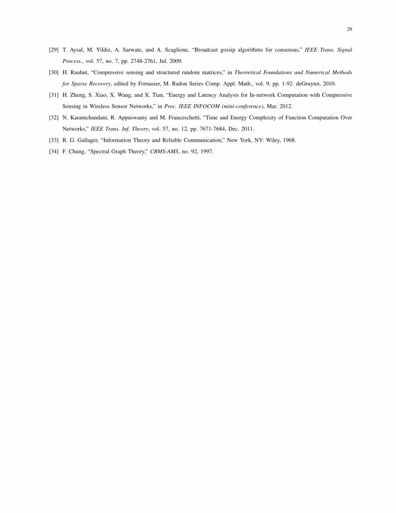
contains Θ(log n) nodes with high probability. In each cell, a node is randomly selected as a

cell head. A spanning tree is formed, as shown in Fig. 2, where the sink is designated as the

root, the vertices include all the cell heads and the links connect only between the adjacent

cell heads. The proposed protocol is composed of two protocols: an intra-cell protocol and an

inter-cell protocol. In the intra-cell protocol, a node in each cell is designated as a cell head

to collect the data from the neighboring nodes within the same cell. In the inter-cell protocol,

each cell head gets values from its children, aggregates and computes them, and then forwards

the results to its parent. Finally, the sink recovers all the raw data from the computation results.

Now we present the protocol in details.

1) Intra-cell protocol:

In each cell, a node is randomly designated as a cell head. We denote Hj as the cell

head and nj as the number of nodes in the jth cell Cj where j = 1, · · · , l. For each time

slot, the nodes in the jth cell take turns to transmit their data to the cell head Hj . Note

that there are nj = Θ(log n) nodes in each cell, and thus the cell head Hj has Θ(log n)

measurements including its own measurement in its transmitting buffer.

2) Inter-cell protocol: Now we describe how to compute the ith multiround random linear

function Fi, i.e., the ith random projection, and deliver computation results along the

11

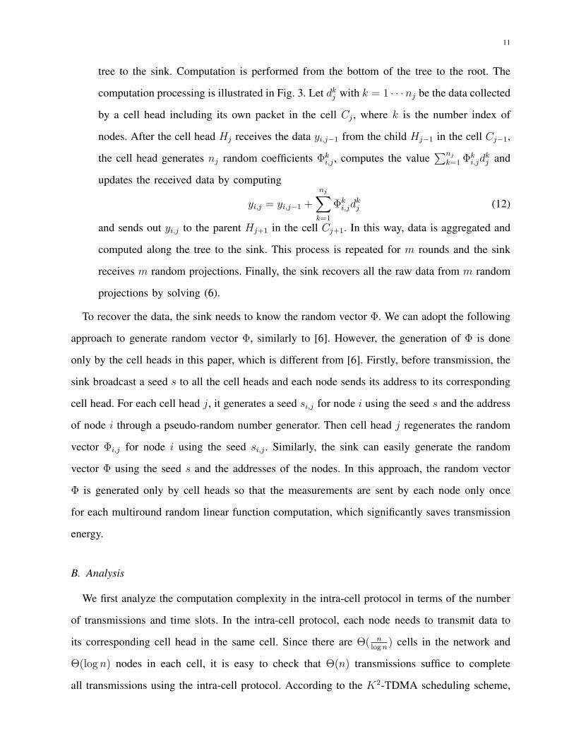
tree to the sink. Computation is performed from the bottom of the tree to the root. The

computation processing is illustrated in Fig. 3. Let dkj with k = 1 · · ·nj be the data collected

by a cell head including its own packet in the cell Cj , where k is the number index of

nodes. After the cell head Hj receives the data yi,j−1 from the child Hj−1 in the cell Cj−1,

the cell head generates nj random coefficients Φki,j , computes the value

∑nj

k=1Φki,jd

kj and

updates the received data by computing

yi,j = yi,j−1 +

nj∑k=1

Φki,jd

kj (12)

and sends out yi,j to the parent Hj+1 in the cell Cj+1. In this way, data is aggregated and

computed along the tree to the sink. This process is repeated for m rounds and the sink

receives m random projections. Finally, the sink recovers all the raw data from m random

projections by solving (6).

To recover the data, the sink needs to know the random vector Φ. We can adopt the following

approach to generate random vector Φ, similarly to [6]. However, the generation of Φ is done

only by the cell heads in this paper, which is different from [6]. Firstly, before transmission, the

sink broadcast a seed s to all the cell heads and each node sends its address to its corresponding

cell head. For each cell head j, it generates a seed si,j for node i using the seed s and the address

of node i through a pseudo-random number generator. Then cell head j regenerates the random

vector Φi,j for node i using the seed si,j . Similarly, the sink can easily generate the random

vector Φ using the seed s and the addresses of the nodes. In this approach, the random vector

Φ is generated only by cell heads so that the measurements are sent by each node only once

for each multiround random linear function computation, which significantly saves transmission

energy.

B. Analysis

We first analyze the computation complexity in the intra-cell protocol in terms of the number

of transmissions and time slots. In the intra-cell protocol, each node needs to transmit data to

its corresponding cell head in the same cell. Since there are Θ( nlogn

) cells in the network and

Θ(log n) nodes in each cell, it is easy to check that Θ(n) transmissions suffice to complete

all transmissions using the intra-cell protocol. According to the K2-TDMA scheduling scheme,

12

concurrent transmissions can occur in different super cells, where each time slot is allocated to

each node. It is easy to know that there are Θ(K2 log n) nodes in each super cell. Therefore,

it requires Θ(K2 log n) time slots for all the transmissions in this stage. By Lemma 2, K is a

constant. Therefore, the intra-cell protocol can be completed in this stage in T1 = Θ(log n) time

slots using E1 = Θ(n) transmissions.

Next we consider the computation complexity in the inter-cell protocol. There are Θ( nlogn

)

nodes in the spanning tree which only consists of cell heads. To compute one random projection,

each cell head transmits only once. Thus, it requires Θ( nlogn

) transmissions. Therefore, Θ( mnlogn

)

transmissions in total are needed to compute m random projections. Now we consider the cell

scheduling for the inter-cell protocol. Note that communication occurs only among cell heads

in this stage. The scheduling starts from the bottom of the tree since the nodes at a level can

not be scheduled before all the children at this level are scheduled. We note that each cell head

has a bounded number of children. Also, each cell head has a bounded number of interfering

neighbors. Therefore, the time required to schedule all the cell heads at one level is a constant.

The depth of the tree is Θ(√

nlogn

). Hence, the inter-cell protocol requires Θ(√

nlogn

) time slots to

compute one random projection. Therefore, to compute m random projections, Θ(m√

nlogn

) time

slots are needed. Thus, this stage requires E2 = Θ( mnlogn

) transmissions and T2 = Θ(m√

nlogn

)

time slots.

For signal recovery, m should satisfy the condition m = Ω(log n). Therefore, the bottleneck of

the computation complexity of the proposed protocol lies in the inter-cell protocol. Summarizing

the above analysis, we can conclude that the proposed protocol requires E = E1+E2 = Θ( mnlogn

)

transmissions and T = T1 + T2 = Θ(m√

nlogn

) time slots. Therefore, we have the following

theorem:

Theorem 1: In a random geometric network, the multiround random linear function can be

computed with Θ( mnlogn

) transmissions and Θ(m√

nlogn

) time slots.

C. Discussion

To compare with the above result, we consider the traditional transmission approach, where

the nodes collect data and forward it to the sink without any computations being performed at

the intermediate nodes. The data is directly transported to the sink via multihop transmissions

13

through the shortest path routing strategy. This approach corresponds to computing the identity

function [4]. The computation complexity of this approach has been analyzed in [5], which

is shown that it requires Θ(n√n/ log n) transmissions and Θ(n) time slots for computing the

max function. The traditional transmission approach allows all the raw data to be delivered

directly at the sink without any further recovery algorithm. In contrast, the proposed protocol

firstly performs computation at the cell heads and then reconstructs the raw data with a recovery

algorithm. From Theorem 1, we find that the CS-based approach can save energy and reduce

latency for data gathering by a factor of Θ(√n lognm

) respectively when m = O(√n log n). It can

be noted that the advantage of the proposed approach over the traditional transmission approach

can be exploited by the fact that the measurements in a dense sensor network are highly correlated

and the correlation can be further utilized by the approach of compressive sensing. However,

we also notice that the CS-based approach may be not energy efficient when m = ω(√n log n)

compared with the traditional transmission approach.

V. TREE-BASED COMPUTATION PROTOCOL WITH COMPRESSIVE SENSING IN NOISY

RANDOM NETWORKS

In this section, we present a protocol for computing the multiround random linear function

in noisy wireless networks. We adopt a noisy broadcast model, where each node can broadcast

measurements to the other nodes through independent binary symmetric channels with error

probability ϵ. This model has been commonly used in function computation in noisy random

networks [16]–[19]. The cell partition method and the cell scheduling scheme adopted in this

section are the same as those described in Section IV. The proposed protocol is also composed

of two protocols: an intra-cell protocol and an inter-cell protocol.

A. Protocol

The intra-cell protocol is responsible for collecting measurements from all the nodes in each

cell over a noisy channel. The intra-cell protocol works in four stages, which follows some

similar ideas from the work in [18].

Intra-cell protocol:

14

1) For any cell Cj , a node is randomly selected as a cell head Hj . Denote nj as the number

of nodes in the cell Cj , where nj = Θ(log n). Each node in the cell Cj takes turns to

broadcast its measurement 10λ(log log n) times, where λ = − log(4ϵ(1 − ϵ)). Thus, each

node in the cell Cj will receive 10λ(log log n) noisy copies from the other nodes.

2) Each node in the cell Cj decodes the measurements received from the other nodes using

a majority rule and gets nj estimates including its own measurement.

3) Randomly select lj =nj

log lognnodes in each cell. Each selected node concatenates its

estimates into a word and codes it with a codeword of length O(k1nj), and then transmits

it to the cell head, where k1 is a constant. Then the cell head receives each codeword

and decodes it. We will show that there exists a constant k1 such that each selected node

decodes the codeword correctly with high probability.

4) Each cell head makes the final estimates for the received measurements by using a majority

rule.

At the end of stage 4, the information is accumulated at the cell head. Before the inter-cell

protocol is executed, a spanning tree is formed, as shown in Fig. 2. Computation is performed

along the spanning tree, and finally all the computation results are aggregated at the sink. The

inter-cell protocol is executed as follows:

Inter-cell protocol:

1) Each cell head computes the value yi,j in (12) with the information from its own cell and

its child cell heads. The computation of the value yi,j is executed the same as the inter-cell

computation protocol in noiseless networks. Note that before computing the value yi,j ,

each cell head decodes the information from its child cell heads.

2) Each cell head encodes the value yi,j with a codeword of length O(k2 log n) and transmits

it to the parent cell head, where k2 is a constant.

The above inter-cell computation protocol is repeated for m times and the sink obtains m random

projections. Finally, the sink reconstruct data from these computation results using a recovery

algorithm.

15

B. Analysis

We now analyze the computation complexity in the intra-cell protocol as follows. In the intra-

cell protocol, it requires Θ(n · 10λ(log log n)) transmissions and Θ(K2 · log n · 10

λ(log log n)) time

slots in stage 1 since each node needs to transmit its measurement to its corresponding cell head

for 10λ(log log n) times and transmissions are scheduling under the K2-TDMA scheme. In stage 3,

the total number of transmissions is Θ(nj

log logn·k1nj · n

logn) = Θ( n logn

log logn) and it requires Θ(

K2nj ·nj

log logn)

time slots. Therefore, the intra-cell protocol can be completed in Θ(10n log lognλ

+ n lognlog logn

), i.e.,

Θ( n lognlog logn

) transmissions and Θ( log2 nlog logn

+ 8K2 logn log lognλ

) i.e., Θ( log2 nlog logn

) time slots.

We now consider the computation complexity in the inter-cell protocol. Note that there are

Θ( nlogn

) cell heads in the spanning tree. To compute one random projection, each cell head

transmits once. Therefore, it requires Θ(k2 log n · nlogn

), i.e., Θ(n) transmissions for the sink to

compute one random projections. Hence, to compute m random projections, it requires Θ(mn)

transmissions in total for the inter-cell protocol. The cell scheduling for the inter-cell protocol is

the same as that in noiseless networks, which also starts from the bottom of the tree. Therefore,

Θ(K2mk2 log n√

nlogn

) time slots are needed to compute m random projections. Thus, the inter-

cell protocol requires Θ(mn) transmissions and Θ(m√n log n) time slots.

We further consider the error probability for the intra-cell protocol and the inter-cell protocol,

respectively. For the intra-cell protocol, by Lemma 3, the error probability that each estimate is

decoded is at most p1 = nje−5 log logn = e−4 log logn in stage 2. In stage 3, by Lemma 4, it is easy

to check that there exists a codeword of length k1nj such that the error probability that each

cell head decodes the message is at most p2 = e−4nj = e−4 logn. Therefore, we can bound the

probability that each measurement can be decoded correctly by the cell head at the end of stage

4 in the intra-cell protocol as follows.

Pr(a measurement is decoded correctly)

≥ 1− (4(p1 + p2)(1− (p1 + p2)))nj

2 log logn

≥ 1− (4(e−4 log logn + e−4 logn))logn

2 log logn

≥ 1− (4(e−4 log logn + e−4 log logn))logn

2 log logn

≥ 1− 1

n2, for n large enough

(13)

Thus, the total probability that all the cell heads decode all the measurements correctly is at

16

least 1− nlogn

· 1n2 =1− 1

n logn.

For the inter-cell protocol, by Lemma 4, the probability of a codeword can be correctly decoded

by its parent cell head is at least

Pr(a codeword is decoded correctly)

≥ 1− e−k2 logn

(14)

By the union bound, the probability that the sink can recover the data from m random projections

Pr(the sink recovers the data correctly)

≥ 1− mn

log ne−k2 logn

≥ 1− m

nk2−1 log n

(15)

When k2 ≥ 2 and m ≪ n, we can conclude that the sink can recover the data correctly with

high probability.

From the above results, we show that the bottleneck of the complexity of the computation

protocol also lies in the inter-cell protocol when m = Ω(log n). Thus, the inter-cell protocol

needs Θ(mn) transmissions and Θ(m√n log n) time slots. Summarizing the above analysis, we

can have the following theorem

Theorem 2: In a noisy random network , the proposed computation protocol requires Θ(mn)

transmissions and Θ(m√n log n) time slots.

C. Discussion

From Theorem 2, we observe that the number of transmissions of the proposed computation

protocol in noisy networks is up to a factor Θ(log n) with respect to that in noiseless networks

which is Θ( mnlogn

). Furthermore, comparing the result with that of a general protocol proposed in

[19] for computing the identity function, which needs Θ( n2

logn) transmissions, we show that our

proposed protocol can save energy by a factor of Θ( nm logn

). Even though we compare with the

result of a more efficient protocol proposed in [19] (corresponding to the traditional transmission

approach), where the identity function can be computed correctly with high probability at the

cost of Θ(n√

nlogn

) transmissions, we also show that a gain of Θ(√n

m√logn

) can be achieved as

long as m = O(√

nlogn

). The distinction between our protocol and the protocol in [19] is that

the raw data can be reconstructed with a recovery algorithm in our protocol while the data is

directly transmitted to the sink without using any recovery algorithm.

17

VI. GOSSIP-BASED COMPUTATION PROTOCOL WITH COMPRESSIVE SENSING IN RANDOM

NETWORKS

In the above section, we have presented tree-based protocols for computing the multiround

random linear function in both noiseless and noisy networks. However, the tree-based protocol

suffers from some drawbacks. First, the tree-based protocol needs to maintain the structure of

the tree, which leads to energy consumption overhead. Furthermore, the tree-based protocol

is susceptible to the failure of nodes or links. Any failure of nodes or links will lead to the

topology of the WSN changing and the structure of the tree has to be rebuilt, thus increasing

energy consumption. Moreover, the computation results are not resilient to the failure of nodes

or links. Specially, the failure of the link to the sink node will cause the loss of the computation

results.

To overcome the problems we addressed above, we study a gossip-based protocol for comput-

ing the multiround random linear function in this section. In contrast to the tree-based protocol,

where the computation results are only available on the sink node, the proposed gossip-based

protocol spreads the information over the network. Thus, each sensor node will know the

computation results although the computation results may not always be accurate. Therefore,

the gossip-based protocol provides a more robust approach to the failure of nodes or links than

the tree-based protocol. In this section, we will detail the proposed gossip-based computation

protocol and analyze the performance of the protocol in terms of energy consumption and latency.

A. Protocol

The proposed protocol combines broadcast gossip algorithm with cell scheduling. The cell

scheduling scheme described in Section III is adopted in the proposed protocol. We first describe

how the tth random projection yt is computed and spread to each node. The protocol operates

as follows: Firstly every node obtains its measured value xi at a sampling instance. At each

time slot, one cell in a super cell actives and one node in the cell is randomly selected as a

cell head. The cell head broadcasts a message within distance r(n) from it, where r(n) is the

transmission range. Once neighboring nodes receive the message, a group is formed with the cell

head as group head and neighboring nodes as group members. And then the neighboring nodes

18

compute ωi = nΦi,txi where Φi,t are i.i.d. random variables which take the values of ±1/√n

with probability 1/2, and transmit the results to the group head. The group head collects all

the values from these neighboring nodes, computes the average value and broadcasts it to the

neighboring nodes. The neighboring nodes receive the average value and update their values with

it. In a super cell, each cell takes turns to be active and performs the same gossip algorithm.

By cell scheduling, the gossip algorithm can be simultaneously performed in different super

cells, which also speeds up convergence rate. Algorithm 1 gives a description of gossip-based

algorithm in a cell for computing the tth random projection. When the computation results are

within some desired accuracy range, the gossip algorithm stops and continues to compute the

next random projection. When all the computations for m random projections finish, the sink

can query any node for m random projections to recover an estimation of the signal x by solving

the optimization (7).

In order to reconstruct the signal x, the sink needs to know the random vector Φ. Similarly,

we can adopt the approach as described in the tree-based protocol. Differently from the tree-

based protocol where only the cell heads need to generate random vectors for the nodes within

the same cell, each node should generate its own random vector in the gossip-based protocol.

Therefore, before invocation of the gossip algorithm, the sink broadcasts a seed s. Each node i

generates another seed si using the seed s and its address through the pseudo-random number

generator. Then node i regenerates the random vector Φi using the seed si. Finally, the sink can

easily generate the random vector Φ using the seed s and the addresses of the nodes.

Algorithm 1 Gossip-based Computation Algorithm.1: When a cell C is active, one node within it is randomly selected as a cell head H;

2: The cell head H broadcasts a message to the neighboring nodes;

3: Each neighboring node i receives the message and sends the result ωi = nΦi,txi to the cell

head;

4: The cell head H collects all the values, computes the average value v =∑

i ωi/J where J

is the number of the received values, and broadcast it to the neighboring nodes;

5: The neighboring nodes receive the value v and update their values ωi with v;

19

B. Analysis

In this section, we analyze the performance of the gossip-based protocol in terms of energy

consumption and latency. The analysis of the proposed protocol is based on the work [25].

However, we consider the transmission scheduling and compute the multiround random linear

function in our paper, which make our analysis different. Before proceeding our analysis, we

present some preliminaries.

Definition 2: Consider a connected undirected graph G(V,E) with n nodes. Let x = (x1, · · · , xn)

denote the measured value vector of n nodes, where xi is the measured value of node i. To begin

an instance of gossip, each node i initializes the value ωi = nΦi,txi, where Φi,t are i.i.d random

variables which take the values of ±1/√n with probability 1/2. The potential of the graph G

is defined as

ϕ =n∑

i=1

(ωi − ω)2 =n∑

i=1

ωi2 − nω2, (16)

where ω =∑

i ωi/n is the average value on a node. Note that ϕ = 0 if and only if ω =

(ω, · · · , ω).

Definition 3: Convergence Rate. Let ϕ and ϕ′ denote the potential before and after the invo-

cation of the algorithm, respectively. Let δϕ denote the decrement of the potential ϕ− ϕ′. The

convergence rate is defined as δϕ/ϕ.

Let δφi denote the potential decrement of the group gi after executing one iteration of the

algorithm

δφi = (∑j∈gi

ωj2)−

(∑

j∈gi ωj2)

J=

1

J

∑j,k∈gi

(ωj − ωk)2, (17)

where J is the number of nodes in the group gi.

Furthermore, we introduce some linear algebraic concepts in this paper which are used in

our analysis. Let A denote the adjacency matrix of G and D denote the diagonal matrix (di,i)

where di,i is the degree of node i. The matrix L = D − A is the Laplacian Matrix of G. The

eigenvalues of L are 0 = λ1 < λ2 ≤ · · · ≤ λn. The eigenvalue λ2 is the algebraic connectivity

of G.

As mentioned before, the K2-TDMA scheduling scheme is adopted in our algorithm. For each

time slot, the cells with the same color are active and a node in each active cell is randomly

20

selected as a cell head. The number of simultaneously active group is n8K2 logn

. Therefore, the

probability that the node i is selected as a cell head to form a group gi at one time slot is

Pi =1

8K2 logn.

Lemma 6: The convergence rate

E(δϕ

ϕ) ≥ λ2

8K2dm log n(18)

where dm is the maximum degree of the graph G.

Proof:

E(δϕ) =∑i∈V

Pr(i ∈ gi)× (δφi)

=∑i∈V

Pi ×1

di,i + 1

∑j,k∈gi

(ωj − ωk)2

≥∑i∈V

1

8K2dm log n×∑j,k∈gi

(ωj − ωk)2,

(19)

where we use di,i + 1 ≈ di,i ≤ dm. Note that ϕ =∑

i∈V (ωi − ω)2. Therefore,

E(δϕ

ϕ) ≥ 1

8K2dm log n

∑j,k∈V (ωj − ωk)

2∑i∈V (ωi − ω)2

=1

8K2dm log n

(∑j,k∈V ((ωj − ω)− (ωk − ω))2∑

i∈V (ωi − ω)2

).

(20)

Let zi = ωi − ω and z = (z1, · · · , zn)T . Hence,

E(δϕ

ϕ) ≥ 1

8K2dm log n

(∑j,k∈V (zj − zk)

2∑ni=1 zi

2|

n∑i=1

zi = 0, z = 0

)

≥ 1

8K2dm log n

(zTLzzT z

|n∑

i=1

zi = 0, z = 0

).

(21)

Since∑n

i=1 zi = 0, z is orthogonal to the eigenvector u = (1, · · · , 1) of the matrix L, which

corresponds to the eigenvalue λ1. Then, using the Courant-Fischer Minimax Theorem [8]

λ2 = minz

(zTLzzT z

| z ⊥ u, z = 0

), (22)

it follows that

E(δϕ

ϕ) ≥ λ2

8K2dm log n. (23)

For convenience, we assume that

γ =λ2

8K2dm log n. (24)

Lemma 7: Let m1,m2, . . . ,mk be the independent random variables representing the simul-

21

taneous group distributions after the invocation of the algorithm at iteration 1, 2, . . . , k. Let

ϕ1, ϕ2, . . . , ϕk be the random variables representing the potentials after the invocation of the

algorithm at iteration 1, 2, . . . , k. Let Emk(ϕk) be the expected value of ϕk computed over all

possible group distributions at iteration k given the potential ϕk−1 at the previous iteration

k − 1. Let E(ϕk) be the expected value of ϕk computed over all possible group distribution to

m1, . . . ,mk, given the initial potential ϕ0. We have E(ϕk) ≤ (1− γ)kϕ0.

Proof: From Lemma 6, Emk(ϕk) ≤ (1− γ)ϕk−1.

E(ϕk) = Em1,m2,...,mk(ϕk)

= Em1(Em2(· · ·Emk−1(Emk

(ϕk))))

≤ (1− γ)Em1(Em2(· · ·Emk−1(ϕk−1)))

...

≤ (1− γ)kϕ0.

(25)

Let ϕk be the potential after the invocation of the algorithm at the iteration k. If ϕk ≤ ε2, then

the algorithm stops. Now we derive the bound of the number of iterations that the algorithm

requires before it stops.

By Lemma 7,

E(ϕk) ≤ (1− γ)kϕ0 ≤ ε2. (26)

Taking logarithms on the two right terms and applying the inequality − ln(1 − γ) ≥ γ for

−1 ≤ γ < 1, we obtain

k ≥ 1

γlog(

ϕ0

ε2). (27)

Also,

ϕ0 =n∑

i=1

(nΦi,txi)2 − n(

1

n

n∑i=1

nΦi,txi)2

= n

n∑i=1

xi2 − n(

n∑i=1

Φi,txi)2.

(28)

By the fact that Φi,t is a Rademacher sequence and Lemma 5, we have

n(n∑

i=1

Φi,txi)2 ≤ 23/4e−1 · 2

n∑i=1

x2i . (29)

22

Since the signal x is compressible , x has the finite energy. By orthonormality and (3),

||x||22 = ||θ||22 =n∑

i=1

xi2 ≤ R2

n∑i=1

i−2/p. (30)

The summation∑n

i=1 i−2/p is Riemann zeta function which converges to a constant when 0 <

p ≤ 1. Thus, ϕ0 ≤ n∑n

i=1 xi2 = O(n). Assuming that the algorithm stops when the potential ϕ

reaches at a small constant value ε, so ε2 = O(1). By Markov inequality,

Pr(ϕk > ε2) <E(ϕk)

ε2≤ (1− γ)kϕ0

ε2. (31)

Therefore, we can choose k = cγlog(ϕ0

ε2), where c ≥ 2, such that

Pr(ϕk > ε2) < e− log(ϕ0ε2

)c ϕ0

ε2= (

ε2

ϕ0

)c−1 −→ 0. (32)

Thus,

Pr(ϕk ≤ ε2) ≥ 1− (ε2

ϕ0

)c−1 −→ 1. (33)

Therefore, with high probability, the number of iterations requires

k = O

(c

γlog(

ϕ0

ε2)

). (34)

Furthermore, it is shown that λ2 is bounded by the following function of the diameter diam(G)

of the graph [29]:4

n · diam(G)≤ λ2 ≤

8dmdiam(G)2

log22 n. (35)

For the random geometric graph, to guarantee full connectivity, dm = Θ(log n). The diameter

of the the random geometric graph is defined as the number of hops from one corner to the

diagonally opposite corner, which is Θ(√n/ log n) [29], so the bounds of λ2 are

Ω(

√log n

n3/2) = λ2 = O(

log4 n

n). (36)

Combining (24), (34) and (36), we can get the following lower bound and upper bound of the

computation iterations

Ω(n

log n) = k = O(n3/2(log n)5/2). (37)

The above result is only for computing one random projection. Furthermore, for each round of

algorithm, each cell head needs Θ(log n) time slots to collect the data from the neighboring

nodes in the group. Hence, to compute m random projections, the total number of time slots

needed is O(km log n). Thus, we have the following theorem:

Theorem 3: Given a connected undirected graph G(V,E), the bounds of the total number of

time slots Tg needed for computing m random projections in a node within an accuracy ε = O(1)

23

are

Tg = Ω(mn) (38)

Tg = O(mn3/2(log n)7/2). (39)

We now consider the energy consumption by the number of transmissions for computing random

projections. We have the following theorem:

Theorem 4: Given a connected undirected graph G(V,E), the total expected energy consump-

tion Eg in terms of number of transmissions needed for computing m random projections in a

node within an accuracy ε = O(1) is

E(Eg) = Ω(mn2

log n) (40)

E(Eg) = O(mn5/2(log n)5/2). (41)

Proof: Since there are Θ( nlogn

) groups simultaneously compute random projections for each

iteration, the total expected number of transmissions needed for computing m random projections

is E(Eg) = Tg ×Θ( nlogn

). By Theorem 3, we obtain the above theorem.

C. Gossip-based computation protocol with link failures

In this subsection, we consider the case when wireless links may fail while gossip-based

computation protocol is being performed. We assume that the failures of wireless links occur

before the invocation of gossip algorithm. Thus, nodes may be unable to update their information

with group heads during the failures of links. We can obtain the performance of the gossip-based

computation protocol in the case of link failures along the line of the above analysis. We model a

wireless sensor network with link failures as the graph G′, which can be regarded as a subgraph

of G. Combining (24), (34) and replacing G by G′ , we can obtain the number of iterations for

the case of link failures

k′ = O

(d(G′) log n

λ2(G′)log(

ϕ

ε2)

)(42)

where d(G′) denotes the maximum degree of the graph G′ and λ2(G′) denotes the connectivity

of the graph G′. Similarly, the performance of the computation protocol under link failures

can be obtained following the above analysis in the case without link failures. However, from

(42) we can see that the performance is dependent on the network condition with respect to

24

link failures. Therefore, we will investigate the performance with different probabilities of link

failures through simulations.

D. Discussion

From Theorems 3 and 4, we know that the upper and lower bounds of energy consumption

and latency are not tight. They differ by a√n factor if the logarithmic terms are ignored. The

difference is due to the fact that the bounds of the geometric connectivity λ2 of graph G are not

tight. Reference [29] discusses the possible approach to tighten this upper bound. However, this

goes beyond our paper. Furthermore, we compare the performance of our gossip-based approach

with the performance of the scheme using randomized gossip [6], where a node randomly selects

one neighboring node to exchange random measurements and compute the average value for each

iteration of computation. In [6], it has been shown that the number of transmissions needed to

compute m random projections is Θ(mn2) within an accuracy ε = O(1) . In our work, we show

that our broadcast gossip-based approach requires Ω(mn2

logn) transmissions, which indicates that

our approach requires fewer transmissions than the randomized gossip-based approach. However,

comparing with the tree-based computation protocol which needs only Θ( mnlogn

) transmissions

for one round of computation, the gossip-based protocol is less efficient in energy consumption.

Thus, the robustness achieved in such a protocol is at the cost of extra energy consumption.

VII. NUMERICAL SIMULATIONS

In this section, we present some simulations to compare the performance of the proposed

protocols for function computation. We firstly discuss the compressibility of a sensing field

and demonstrate that the sensing field can be represented by an orthonormal basis using the

eigenvectors of the graph Laplacian in random geometric network. We also study the performance

of the proposed computation protocols for both the tree-based protocol and the gossip-based

protocol. Finally, we investigate the performance of the tree-based computation protocol and the

gossip-based computation protocol over unreliable wireless networks.

25

A. Compressibility of a piece-wise smooth field

We consider a random geometric network where n nodes are randomly and independently

distributed in a unit square area. The transmission range is set to be 8√log n/n. Since the

network topology of random geometric network is irregular and we can not use the transform

basis such as wavelet transform basis to sparsify the sensing data, here we use the eigenvectors

of the graph Laplacian as an orthonormal basis. The Laplacian Matrix L of the graph G(V,E)

is defined as follows [34]:

Li,j =

−1 if (i, j) ∈ E

di,i if i = j

0 otherwise,

(43)

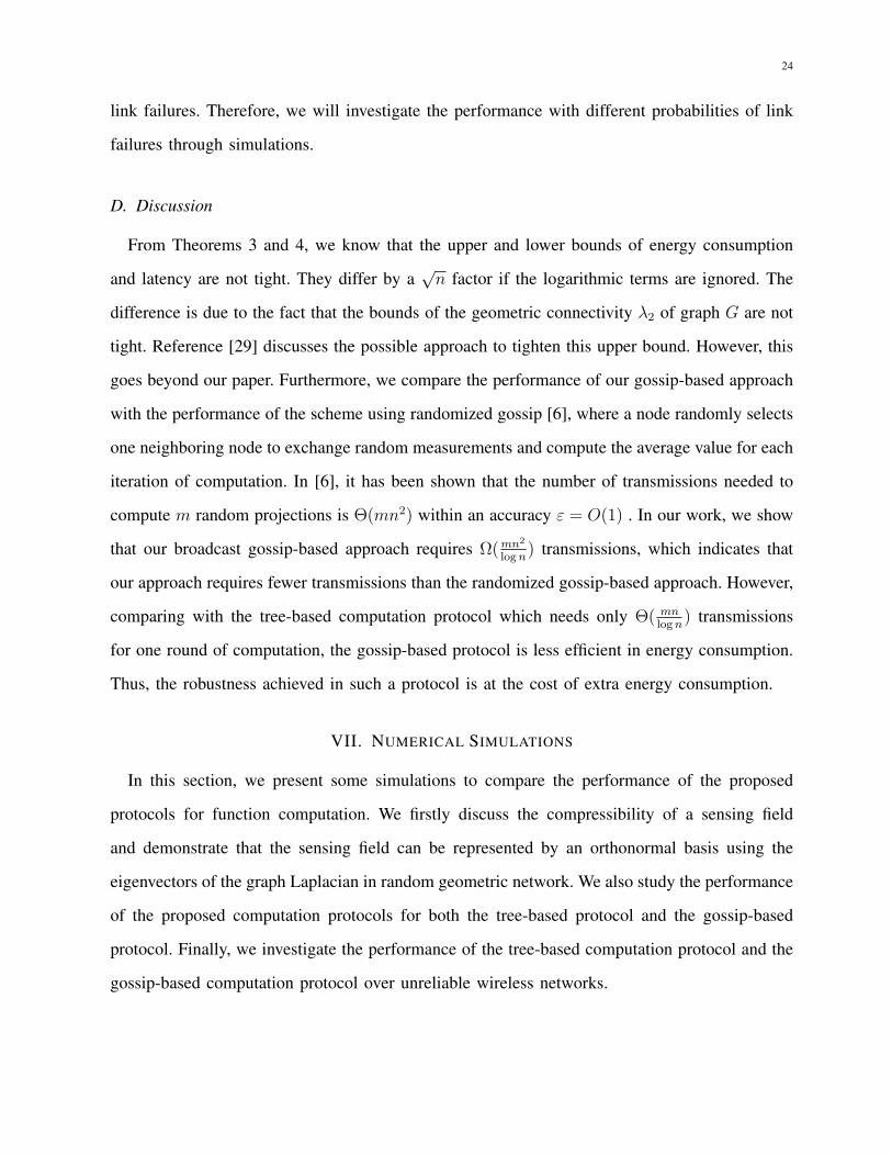
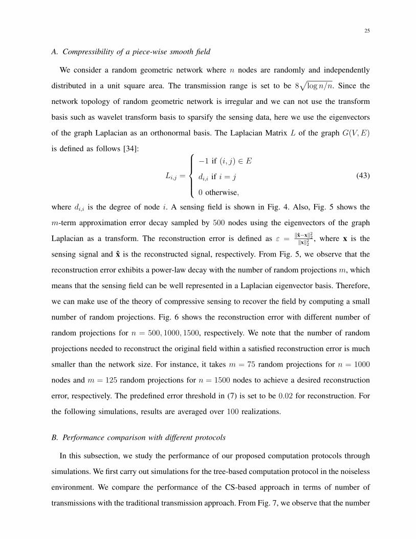
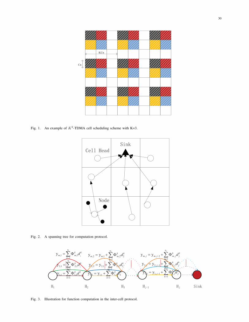
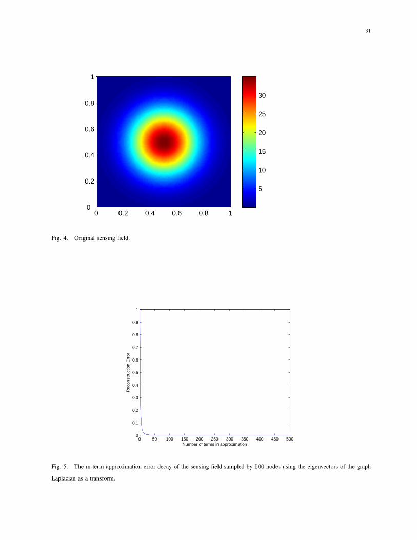
where di,i is the degree of node i. A sensing field is shown in Fig. 4. Also, Fig. 5 shows the

m-term approximation error decay sampled by 500 nodes using the eigenvectors of the graph

Laplacian as a transform. The reconstruction error is defined as ε =∥x−x∥22∥x∥22

, where x is the

sensing signal and x is the reconstructed signal, respectively. From Fig. 5, we observe that the

reconstruction error exhibits a power-law decay with the number of random projections m, which

means that the sensing field can be well represented in a Laplacian eigenvector basis. Therefore,

we can make use of the theory of compressive sensing to recover the field by computing a small

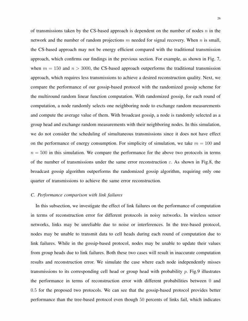
number of random projections. Fig. 6 shows the reconstruction error with different number of

random projections for n = 500, 1000, 1500, respectively. We note that the number of random

projections needed to reconstruct the original field within a satisfied reconstruction error is much

smaller than the network size. For instance, it takes m = 75 random projections for n = 1000

nodes and m = 125 random projections for n = 1500 nodes to achieve a desired reconstruction

error, respectively. The predefined error threshold in (7) is set to be 0.02 for reconstruction. For

the following simulations, results are averaged over 100 realizations.

B. Performance comparison with different protocols

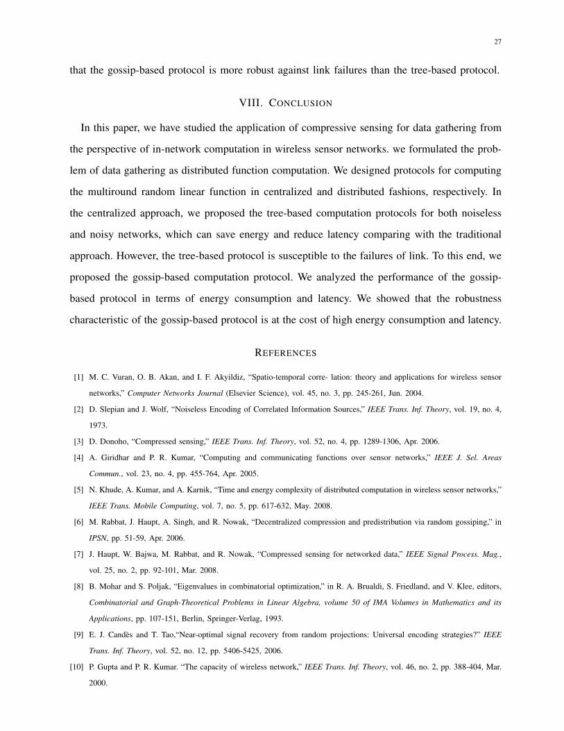
In this subsection, we study the performance of our proposed computation protocols through

simulations. We first carry out simulations for the tree-based computation protocol in the noiseless

environment. We compare the performance of the CS-based approach in terms of number of

transmissions with the traditional transmission approach. From Fig. 7, we observe that the number

26

of transmissions taken by the CS-based approach is dependent on the number of nodes n in the

network and the number of random projections m needed for signal recovery. When n is small,

the CS-based approach may not be energy efficient compared with the traditional transmission

approach, which confirms our findings in the previous section. For example, as shown in Fig. 7,

when m = 150 and n > 3000, the CS-based approach outperforms the traditional transmission

approach, which requires less transmissions to achieve a desired reconstruction quality. Next, we

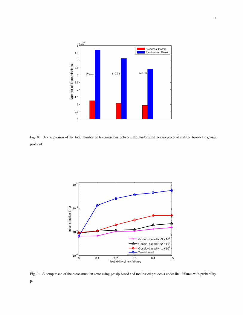
compare the performance of our gossip-based protocol with the randomized gossip scheme for

the multiround random linear function computation. With randomized gossip, for each round of

computation, a node randomly selects one neighboring node to exchange random measurements

and compute the average value of them. With broadcast gossip, a node is randomly selected as a

group head and exchange random measurements with their neighboring nodes. In this simulation,

we do not consider the scheduling of simultaneous transmissions since it does not have effect

on the performance of energy consumption. For simplicity of simulation, we take m = 100 and

n = 500 in this simulation. We compare the performance for the above two protocols in terms

of the number of transmissions under the same error reconstruction ε. As shown in Fig.8, the

broadcast gossip algorithm outperforms the randomized gossip algorithm, requiring only one

quarter of transmissions to achieve the same error reconstruction.

C. Performance comparison with link failures

In this subsection, we investigate the effect of link failures on the performance of computation

in terms of reconstruction error for different protocols in noisy networks. In wireless sensor

networks, links may be unreliable due to noise or interferences. In the tree-based protocol,

nodes may be unable to transmit data to cell heads during each round of computation due to

link failures. While in the gossip-based protocol, nodes may be unable to update their values

from group heads due to link failures. Both these two cases will result in inaccurate computation

results and reconstruction error. We simulate the case where each node independently misses

transmissions to its corresponding cell head or group head with probability p. Fig.9 illustrates

the performance in terms of reconstruction error with different probabilities between 0 and

0.5 for the proposed two protocols. We can see that the gossip-based protocol provides better

performance than the tree-based protocol even though 50 percents of links fail, which indicates

27

that the gossip-based protocol is more robust against link failures than the tree-based protocol.

VIII. CONCLUSION

In this paper, we have studied the application of compressive sensing for data gathering from

the perspective of in-network computation in wireless sensor networks. we formulated the prob-

lem of data gathering as distributed function computation. We designed protocols for computing

the multiround random linear function in centralized and distributed fashions, respectively. In

the centralized approach, we proposed the tree-based computation protocols for both noiseless

and noisy networks, which can save energy and reduce latency comparing with the traditional

approach. However, the tree-based protocol is susceptible to the failures of link. To this end, we

proposed the gossip-based computation protocol. We analyzed the performance of the gossip-

based protocol in terms of energy consumption and latency. We showed that the robustness

characteristic of the gossip-based protocol is at the cost of high energy consumption and latency.

REFERENCES

[1] M. C. Vuran, O. B. Akan, and I. F. Akyildiz, “Spatio-temporal corre- lation: theory and applications for wireless sensor

networks,” Computer Networks Journal (Elsevier Science), vol. 45, no. 3, pp. 245-261, Jun. 2004.

[2] D. Slepian and J. Wolf, “Noiseless Encoding of Correlated Information Sources,” IEEE Trans. Inf. Theory, vol. 19, no. 4,

1973.

[3] D. Donoho, “Compressed sensing,” IEEE Trans. Inf. Theory, vol. 52, no. 4, pp. 1289-1306, Apr. 2006.

[4] A. Giridhar and P. R. Kumar, “Computing and communicating functions over sensor networks,” IEEE J. Sel. Areas

Commun., vol. 23, no. 4, pp. 455-764, Apr. 2005.

[5] N. Khude, A. Kumar, and A. Karnik, “Time and energy complexity of distributed computation in wireless sensor networks,”

IEEE Trans. Mobile Computing, vol. 7, no. 5, pp. 617-632, May. 2008.

[6] M. Rabbat, J. Haupt, A. Singh, and R. Nowak, “Decentralized compression and predistribution via random gossiping,” in

IPSN, pp. 51-59, Apr. 2006.

[7] J. Haupt, W. Bajwa, M. Rabbat, and R. Nowak, “Compressed sensing for networked data,” IEEE Signal Process. Mag.,

vol. 25, no. 2, pp. 92-101, Mar. 2008.

[8] B. Mohar and S. Poljak, “Eigenvalues in combinatorial optimization,” in R. A. Brualdi, S. Friedland, and V. Klee, editors,

Combinatorial and Graph-Theoretical Problems in Linear Algebra, volume 50 of IMA Volumes in Mathematics and its

Applications, pp. 107-151, Berlin, Springer-Verlag, 1993.

[9] E. J. Candes and T. Tao,“Near-optimal signal recovery from random projections: Universal encoding strategies?” IEEE

Trans. Inf. Theory, vol. 52, no. 12, pp. 5406-5425, 2006.

[10] P. Gupta and P. R. Kumar. “The capacity of wireless network,” IEEE Trans. Inf. Theory, vol. 46, no. 2, pp. 388-404, Mar.

2000.

28

[11] E. Kushilevitz and N. Nisan, “Communication Complexity,” Cambridge University Press, 1997.

[12] A. E. Gamal,“Reliable communication of highly distributed information,” in Open Problems in Communication and

Computation, T. M. Cover and B. Gopinath, Eds. Springer-Verlag, pp. 60-62, 1987.

[13] R. G. Gallager, “Finding parity in a simple broadcast network,” IEEE Trans. Inf. Theory, vol. 34, no. 2, pp. 176-180, Mar.

1988.

[14] N. Goyal, G. Kindler, and M. Saks, “Lower bounds for the noisy broadcast problem,” SIAM Journal on Computing, vol.

37, no. 6, pp. 1806-1841, Mar. 2008.

[15] C. Li, H. Dai, and H. Li, “Finding the k largest metrics in a noisy broadcast network,” in Proceedings of the Annual

Allerton Conference on Communication, Control, and Computing, pp. 1184-1190, 2008.

[16] Y. Kanoria and D. Manjunath, “On distributed computation in noisy random planar networks,” in Proceedings of the IEEE

International Symposium on Information Theory (ISIT), pp. 626-630, 2007.

[17] C. Dutta, Y. Kanoria, D. Manjunath, and J. Radhakrishnan, “A tight lower bound for parity in noisy communication

networks,” in Proceedings of the nineteenth annual ACM-SIAM Symposium on Discrete Algorithms (SODA), pp. 1056-

1065, 2008.

[18] L. Ying, R. Srikant, and G. E. Dullerud, “Distributed symmetric function computation in noisy wireless sensor networks,”

IEEE Trans. Inf. Theory, vol. 53, no. 12, pp. 4826-4833, Dec. 2007.

[19] C. Li and H. Dai, “Towards efficient designs for in-network computing with noisy wireless channels,” in Proc. INFOCOM,

Mar. 2010.

[20] C. Luo, F. Wu, J. Sun, and C. W. Chen, “Compressive data gathering for large-scale wireless sensor networks,” in Proc.

ACM Mobicom, pp. 145-156, Sep. 2009.

[21] G. Quer, R. Masiero, D. Munaretto, M. Rossi, J. Widmer, and M. Zorzi, “On the interplay between routing and signal

representation for compressive sensing in wireless sensor networks,” in ITA, Feb. 2009.

[22] S. Lee, S. Pattem, M. Sathiamoorthy, B. Krishnamachari, and A. Ortega, “ Spatially-localized compressed sensing and

routing in multi-hop sensor networks,” in Proc. Third International Conference on Geosensor Networks, vol. 5669, pp.

11-20, Jul. 2009.

[23] S. Lee, S. Pattem, M. Sathiamoorthy, B. Krishnamachari, and A. Ortega, “Compressed sensing and routing in multi-hop

networks,” in USC CENG Technical Report, 2009.

[24] S. Toumpis and A. J. Goldsmith, “Large wireless networks under fading, mobility, and delay constraints,” in Proc. IEEE

INFOCOM, pp. 609-619, Mar. 2004.

[25] J. Y. Chen, G. Pandurangan, and D. Xu, “Robust Computation of Aggregates in Wireless Sensor Networks: Distributed

Randomized Algorithms and Analysis,” IEEE Trans. Parallel and Distributed Systems, vol. 17, no. 9, pp. 987-1000, Sep.

2006.

[26] S. Boyd, A. Ghosh, B. Prabhakar, and D. Shah, “Randomized gossip algorithms,” IEEE Trans. Inf. Theory, vol. 52, no. 6,

pp. 2508-2530, Jun. 2006.

[27] F. Benezit, A. Dimakis, P. Thiran, and M. Vetterli, “Order-Optimal Consensus Through Randomized Path Averaging,”

IEEE Trans. Inf. Theory, vol. 56, no. 10, pp. 5150-5167, Oct. 2010

[28] D. Ustebay, B. N. Oreshkin, M. J. Coates, and M. G. Rabbat, “Greedy gossip with eavesdropping,” IEEE Trans. Signal

Process.,vol. 58, no. 7, pp. 3765-3776, Jul. 2010.

29

[29] T. Aysal, M. Yildiz, A. Sarwate, and A. Scaglione, “Broadcast gossip algorithms for consensus,” IEEE Trans. Signal

Process., vol. 57, no. 7, pp. 2748-2761, Jul. 2009.

[30] H. Rauhut, “Compressive sensing and structured random matrices,” in Theoretical Foundations and Numerical Methods

for Sparse Recovery, edited by Fornasier, M. Radon Series Comp. Appl. Math., vol. 9, pp. 1-92. deGruyter, 2010.

[31] H. Zheng, S. Xiao, X. Wang, and X. Tian, “Energy and Latency Analysis for In-network Computation with Compressive

Sensing in Wireless Sensor Networks,” in Proc. IEEE INFOCOM (mini-conference), Mar. 2012.

[32] N. Karamchandani, R. Appuswamy and M. Franceschetti, “Time and Energy Complexity of Function Computation Over

Networks,” IEEE Trans. Inf. Theory, vol. 57, no. 12, pp. 7671-7684, Dec. 2011.

[33] R. G. Gallager, “Information Theory and Reliable Communication,” New York, NY: Wiley, 1968.

[34] F. Chung, “Spectral Graph Theory,” CBMS-AMS, no. 92, 1997.

30

Cn

KCn

Fig. 1. An example of K2-TDMA cell scheduling scheme with K=3.

Fig. 2. A spanning tree for computation protocol.

1

1,1 ,1

1

yn

k k

m m

k

d

!"1

12,1 2,1

1

yn

k k

k

d

!"1

11,1 1,1

1

yn

k k

k

d

!"

2

,2 ,1 ,2 2

1

y yn

k k

m m m

k

d

! "#2

2,2 2,1 2,2 2

1

y yn

k k

k

d

! "#2

1,2 1,1 1,2 2

1

y yn

k k

k

d

! "#

, , 1 ,

1

y yjn

k k

m j m j m j j

k

d

!

! " #$

2, 2, 1 2,

1

y yjn

k k

j j j j

k

d

!

! " #$

1, 1, 1 1,

1

y yjn

k k

j j j j

k

d

!

! " #$

Fig. 3. Illustration for function computation in the inter-cell protocol.

31

0 0.2 0.4 0.6 0.8 10

0.2

0.4

0.6

0.8

1

5

10

15

20

25

30

Fig. 4. Original sensing field.

0 50 100 150 200 250 300 350 400 450 5000

0.1

0.2

0.3

0.4

0.5

0.6

0.7

0.8

0.9

1

Number of terms in approximation

Rec

onst

ruct

ion

Err

or

Fig. 5. The m-term approximation error decay of the sensing field sampled by 500 nodes using the eigenvectors of the graph

Laplacian as a transform.

32

50 100 150 200 250 3000

0.1

0.2

0.3

0.4

0.5

0.6

0.7

0.8

0.9

Number of random projections

Rec

onst

ruct

ion

Err

or

n=500n=1000n=1500

Fig. 6. Reconstruction error vs. the number of random projections in the network with different number of nodes.

500 1000 1500 2000 2500 3000 3500 4000 4500 50000

0.5

1

1.5

2

2.5x 10

4

Number of Nodes

Num

ber

of T

rans

mis

sion

s

TRCS(M=100)CS(M=150)

Fig. 7. A comparison of the total number of transmissions between the CS-based approach and the traditional transmission

approach in the network.

33

0

0.5

1

1.5

2

2.5

3

3.5

4

4.5

5x 10

7

Num

ber

of T

rans

mis

sion

s

Broadcast GossipRandomized Gossip

ε=0.06ε=0.03ε=0.01

Fig. 8. A comparison of the total number of transmissions between the randomized gossip protocol and the broadcast gossip

protocol.

0 0.1 0.2 0.3 0.4 0.510

−3

10−2

10−1

100

Probability of link failures

Rec

onst

ruct

ion

Err

or

Gossip−based,N=3 × 107

Gossip−based,N=2 × 107

Gossip−based,N=1 × 107

Tree−based

Fig. 9. A comparison of the reconstruction error using gossip-based and tree-based protocols under link failures with probability

p.