Space-Time Coding Schemes for Wireless Communications over ...iwct.sjtu.edu.cn/personal/mxtao/paper/mxtaoPhDthesis.pdf · Space-Time Coding Schemes for Wireless Communications over

Space-Time Coding Schemes for Wireless

Communications over Flat Fading Channels

A PhD Thesis Submitted to The Hong Kong University of Science and Technology

in Partial Fulfillment of the Requirements for the Degree of Doctor of Philosophy

in Electrical and Electronic Engineering

by

Meixia TAO

B.S., Fudan University, 1999

Department of Electrical and Electronic Engineering The Hong Kong University of Science & Technology

Clear Water Bay, Kowloon, Hong Kong

June 2003, Hong Kong

Authorization

I hereby declare that I am the sole author of the thesis.

I authorize the Hong Kong University of Science & Technology to lend this thesis

to other institutions or individuals for the purpose of scholarly research.

I further authorize the Hong Kong University of Science & Technology to

reproduce the thesis by photocopying or by other means, in total or in part, at the request

of other institutions or individuals for the purpose of scholarship research.

Meixia TAO

ii



by

Meixia TAO

This is to certify that I have examined the above PhD thesis

and have found that it is complete and satisfactory in all respects, and that any and all revisions required by

the thesis examination committee have been made.

Prof. Roger S. CHENG (Thesis Supervisor)

Prof. Shihe YANG (Committee Chairman)

Prof. Ross D. MURCH (Committee Member)

Prof. Wai Ho MOW (Committee Member)

Prof. Gary S. H. CHAN (Committee Member)

Prof. Khaled BEN LETAIEF (Acting Head of Department)

Department of Electrical and Electronic Engineering Hong Kong University of Science & Technology

June 2003

iii

To my parents

iv

Acknowledgements

I would like to express my sincere gratitude to my advisor, Prof. Roger S. Cheng, who is

an endless source of enthusiasm, ideas, and patience. It was him who led me into this

exciting area of wireless communications, and has offered me constant encouragement

and advice throughout the last four years. I hope I have learned from him not just his

broad knowledge, but his insights, inspiration, and his way of conducting research.

I especially thank Prof. Khaled Ben Letaief for introducing me to the academic world

before I started my Ph.D. research, and for giving me useful suggestions in my thesis

proposal. I am grateful to Prof. Ross Murch, Prof. Wai Ho Mow, Prof. Gary Chan

(Computer Science Department) and Prof. Xiang-Gen Xia (Chinese University of Hong

Kong) for being on my committee and providing me some constructive comments. I also

would like to thank Prof. Min Yan (Mathematics Department) and Prof. Kunrui Yu

(Mathematics Department) for helping me to solve some mathematical problems.

I gratefully acknowledge all my former and present colleagues in the wireless

research group for creating such a pleasant work environment and for having useful

discussions with me. Particular thanks go to Jason Leung (ASTRI), Daniel So, Zhiyu Xu

(UTStarcom), Yinjun Zhang, Defeng Huang, Xiaoli Chu, Tao Li, Ruly Choi, Sana Sfar,

Nejib Boubaker, and Peter Chan. It is really wonderful to work with them and talk with

them on many subjects.

I owe deepest appreciation to Fan Zhang for his support. He has always been with me

in the whole journey. Without him, this thesis would never have been completed.

Finally, I would like to thank my parents who always encourage and support me in all

of my decisions.

v

Contents

Acknowledgements v

Contents vi

Notations ii

Abbreviations iii

Abstract xv

Chapter 1 Introduction 1

1.1 Promises of Multiple Antennas 1

1.2 Problem Statement and Research Contribution 2

1.2.1 Enhanced Design of Space-Time Codes 3

1.2.2 Intensive Study on Generalized Layered ST Architecture 4

1.2.3 New Schemes for Non-Coherent ST Coding and Modulation 5

1.3 Outline of Thesis 6

1.4 Publication 7

Chapter 2 Preliminaries 9

2.1 System Model 9

2.1.1 Fading Model 9

2.1.2 Signal Model 10

2.1.3 MIMO Channel Model 12

2.1.4 Digital Transmission over MIMO Channels 13

2.2 Performance Measure 14

2.2.1 Channel Capacity 14

2.2.2 Error Probability and Pair-Wise Error Probability 16

2.2.3 Diversity 17

2.2.4 Coding Gain 17

2.3 Relevant MIMO Transmission Schemes 18

2.3.1 Rate-Oriented Layered Space-time Architecture (VBLAST) 18

2.3.2 Diversity-Oriented Space-Time Codes 19

2.3.3 Rate-Diversity-Oriented Space-Time Techniques 23

vi

2.3.4 Non-Coherent Diversity-Oriented (Differential) Unitary Space-

Time Modulation 23

Chapter 3 Improved design of Space-Time Codes at different SNR 25

3.1 System Model 26

3.2 Improved Design Criteria 26

3.2.1 Case 1: α ≈ 1 (Moderate SNR) 27

3.2.2 Case 2: α << 1 (Low SNR) 27

3.2.3 Case 3: α >> 1 (High SNR) 28

3.3 Computer Searched Trellis Codes for Moderate SNR 28

3.3.1 Code Examples 29

3.3.2 Simulation Results 32

3.4 Summary 33

Chapter 4 Diagonal Block Space-Time Coding 35

4.1 System Model and Performance Criteria 36

4.2 Diagonal Block Space-Time Codes 37

4.2.1 Code Structure 37

4.2.2 Performance Measure 38

4.2.3 Discussions on Diagonal Structure 41

4.3 (M, 1) Nonbinary Block Code Construction 42

4.3.1 Optimal Construction for Given Constellations 42

4.3.2 Linear Construction for PSK Modulation 46

4.3.3 Discussions 48

4.4 Simulation Results 49

4.4.1 Comparison with Delay Diversity Codes 49

4.4.2 Comparison with Other Existing Codes 53

4.5 Summary 55

Chapter 5 Generalized Layered Space-Time Architecture 56

5.1 System Model 57

5.1.1 Encoding 58

5.1.2 Decoding 59

5.2 Optimal Power Allocation 60

vii

5.3 Optimal Decoding Order 64

5.4 Interleaved GLST with Hard-Decision Iterative Decoding 68

5.5 Summary 70

Chapter 6 Differential Space-Time Block Codes 73

6.1 System Model 74

6.2 Differential Encoding 75

6.2.1 Data Matrix 75

6.2.2 Transmitted Matrix 76

6.3 Non-Coherent Decoding 76

6.3.1 Optimal Differential Decoder 77

6.3.2 Near Optimal Differential Decoder 78

6.3.3 Optimal DD versus Near Optimal DD 78


6.5 Summary 84

Chapter 7 Trellis-Coded Differential Unitary Space-Time Modulation 86

7.1 Background on DUSTM 87

7.2 System Model and Performance Measure 88

7.2.1 System Model 88

7.2.2 Ideal Interleaver 89

7.2.3 No Interleaver 91

7.3 Code Construction 94

7.3.1 Ideal Interleaver 97

7.3.2 No Interleaver 98


7.5 Extensions to Trellis-Coded Differential Space-Time Block Codes 104

7.6 Summary 106

Chapter 8 Conclusion and Future Work 107

8.1 Conclusion 107

8.2 Future work 109

Bibliography 111

viii

List of Figures

2.1 BPSK and QPSK constellations

2.2 16QAM and 32QAM constellations

2.3 System diagram of MIMO wireless communications.

2.4 QPSK 4-state ST code with 2 transmit antennas

3.1 Performance of the QPSK, 8-state, 2 bit/s/Hz space-time codes with 2 transmit

and 3,4 receive antennas.

3.2 Performance of the 8-PSK, 8-state, 3 bit/s/Hz space-time codes with 2 transmit

and 3, 4 receive antennas.

4.1 Transmitter diagram of the diagonal block space-time codes, “D” denotes one

symbol delay.

4.2 Trellis diagram for the DBST code with QPSK and M = 2.

4.3 SER performance of 8PSK codes with M = 3 transmit antennas over a quasi-static

fading channel.

4.4 SER performance of 8PSK codes with M = 3 transmit antennas over a rapid

fading channel.

4.5 SER performance of 8PSK codes with M = 3 transmit antennas over a time-

varying fading channel with . 05.0=sdTf

4.6 Histogram of the gains shown in Table 4.4.

4.7 FER performance of 8PSK codes with M = 3, 4 transmit antennas over a quasi-

static fading channel.

5.1 Encoder of (interleaved) GLST (a) main layout, (b) HGLST, and (c) DGLST.

5.2 Performance comparison of different power allocation in the (a) (4,4) and (b)

(8,8) GLST systems.

5.3 Performance comparison of optimal ordered decoding in the (a) (4,4) and (b) (8,8)

GLST and BLAST systems.

5.4 Iterative decoding of interleaved GLST (a) main block diagram, (b) sub-block

diagram for the “ST Dec-Enc j’” component.

5.5 Performance of iterative decoding in the (a) (4,4) and (b) (8,8) HGLST systems.

ix

5.6 Performance comparison of interleaved HGLST and interleaved DGLST with

iterative decoding in the (4,4) and (8,8) systems.

6.1 Performance of differential decoding and coherent decoding for G2 with 16QAM

data symbols at M = 2, N = 1, and R = 4 bit/s/Hz.

6.2 Performance of differential decoding and coherent decoding for H4 with 16QAM

data symbols at M = 4, N = 1, and R = 3 bit/s/Hz.

6.3 Performance of differential decoder for G2 with 16PSK and 16QAM data symbols

and cyclic group code at M = 2, N = 1 and R = 4 bit/s/Hz.

6.4 Performance of differential decoder for H4 with 16PSK and 16QAM data symbols

at M = 4, N = 1, and R = 3 bit/s/Hz.

6.5 Performance of differential decoder for H4 with 6PSK data symbols and cyclic

group code at M = 4, N = 1 and R ≈ 2 bit/s/Hz.

7.1 Transmission system diagram of trellis-coded differential unitary space-time

modulation.

7.2 Set-partition of G = ([1 3]; 8).

7.3 Set-partition of G = ([1 7]; 32).

7.4. Trellis diagrams of the codes designed for ideal interleaver case.

7.5 Trellis diagrams of the codes designed for no interleaver case: (a) rate 2/3 4-state

with G = ([1 3]; 8); (b) rate 4/5 16-state with G = ([1 7]; 32).

7.6 BER of rate 2/3 4-state and 8-state G = ([1 3]; 8) TC-DUSTM compared with

uncoded G = ([1 1]; 4) DUSTM, ML differential decoder and ideal interleaver, R

= 1 bit/s/Hz.

7.7 FER of rate 2/3 4-state G = ([1 3]; 8) TC-USTM compared with uncoded G = ([1

1]; 4) USTM, ML coherent decoder and no interleaver, frame length = 100, R = 1

bit/s/Hz.

7.8 FER of rate 2/3 4-state G = ([1 3]; 8) TC-DUSTM compared with uncoded G =

([1 1]; 4) DUSTM and rate 1/2 4-state TC-DPSK, suboptimal differential decoder

and no interleaver, frame length = 102, R = 1 bit/s/Hz.

x

List of Tables

3.1 Space-time codes with QPSK, 4 states, 2 bit/s/Hz.



3.4 Space-time codes with 8PSK, 8 states, 3 bit/s/Hz.

4.1 Optimum block codes used in DBST coding for P = 4 and 8 with PSK modulation

4.2 Optimum block codes used in DBST coding for P = 16 and 32 with PSK/QAM

modulation

4.3 Linear block ring codes used in DBST coding for P = 16, 32, and 64 with PSK

4.4 Operating SNR [dB] at SER = 2 for codes with M = 2 transmit antennas

over a rapid fading channel

410−×

7.1 Determinant distance profile of G = ([1 3]; 8)

7.2 Determinant distance profile of G = ([1 7]; 32)

7.3 Parameters of the codes designed for ideal interleaver case

xi

Notations

Throughout this work scalars are given by lowercase letters (a), vectors by boldface

lowercase letters (a), and matrices by boldface uppercase letters (A). Certain constants or

parameters are given by standard uppercase letters (A).

• 1−=j .

• P(C) is the probability of the event C.

• P(C|D) is the conditional probability of the event C knowing that the event D has

occurred.

• p(a) is the probability density function of the random variable a.

• E[a] is the expectation of the random variable a

• a* is the conjugate of the complex scalar a.

• AT is the transpose of A.

• AH is the complex conjugate transpose of A.

• 0T×N is the T × N zero matrix, the dimension may be dropped if there is no

confusion.

• IM is the M × M identity matrix, the dimension may be dropped if there is no

confusion.

• For a complex number a, )()( aaa jIR +=

• 22 )()( aaa IR += is the absolute value of the complex scalar a.

• ∑∑= =

=N

n

M

mnma

1 1

2,

2A is the squared Euclidean norm of the M × N matrix A with the (m,

n)th entry [A]m,n =am,n.

• rank(A) is the rank of the matrix A.

• det(A) is the determinant of the matrix A.

• tr(A) is the trace of the matrix A.

• diag{a1, a2, …, aM} is an M × M diagonal matrix with diagonal elements a1, a2, …,

aM.

xii

Abbreviations

3G Third Generation Mobile Telephony System

AWGN Additive White Gaussian Noise

BER Bit Error Rate

BLAST Bell-lab LAyered Space-Time architecture

CSI Channel State Information

DBST Diagonal Block Space-Time

DGLST Diagonal Generalized Layered Space-Time architecture

DPSK Differential Phase-Shift-Keying

DSTBC Differential Space-Time Block Codes

DUSTM Differential Unitary Space-Time Modulation

FER Frame Error Rate

GLST Generalized Layered Space-Time architecture

HGLST Horizontal Generalized Layered Space-Time architecture

i.i.d Independent and Identically Distributed

MAP Maximum A Posteriori Probability

MIMO Multiple-Input Multiple-Output

ML Maximum Likelihood

MLSE Maximum Likelihood Sequence Estimator

MMSE Minimum Mean Square Error

PAM Pulse Amplitude Modulation

PWEP Pair-Wise Error Probability

PSK Phase Shift Keying

QAM Quadrature Amplitude Modulation

RF Radio Frequency

Rx Receiver

SER Symbol Error Rate

SISO Single-Input Single-Output

SNR Signal to Noise Ratio

xiii

ST Space-Time

STBC Space-Time Block Code

STC Space-Time Coding

STTC Space-Time Trellis Code

TCM Trellis-Coded Modulation

TC-DPSK Trellis-Coded Differential Phase-Shift-Keying

TC-DUSTM Trellis-Coded Differential Unitary Space-Time Modulation

Tx Transmitter

USTM Unitary Space-Time Modulation

VBLAST Vertical Bell-lab LAyered Space-Time architecture

xiv



by

Meixia TAO

Department of Electrical and Electronic Engineering

The Hong Kong University of Science & Technology

Abstract

The increasing demand for higher data rates and higher quality in wireless

communications has motivated the use of multiple antenna elements at both the

transmitter and the receiver sides in a wireless link. The problem discussed in our

research is the development of fundamental space-time (ST) coding and modulation

methods to achieve the gains provided by multiple antennas, in terms of both improved

robustness of the link and a higher spectral efficiency. We focus on a point-to-point

wireless environment, in which the channel is modeled as flat fading, and channel

knowledge is not available at the transmitter. Several new and improved schemes tailored

for different applications are proposed.

We first consider the design of ST trellis codes that reduce the probability of error

without loss of spectral efficiency. It is found that the typical assumption of high signal-

to-noise ratio (SNR) and, consequently, traditional design criteria are invalid in certain

situations. Analyzing pair-wise error probability, we derive two sets of tighter design

criteria for low and moderate SNR regions, respectively. New ST trellis codes optimized

for moderate SNR are provided via a computer search. To avoid the prohibitively high

complexity of searching for good codes with a larger number of transmit antennas and

higher-level modulation, we introduce a novel systematic code construction method,

diagonal block ST coding. This two-step approach demonstrates promising results at the

commonly assumed high SNR.

xv

We then conduct an intensive study into generalized layered ST architecture that

allows a tradeoff between error probability and spectral efficiency. Our goal is to enhance

the tradeoff by further reducing the error probability. Techniques with no or little increase

in receiver complexity, such as optimal power allocation and optimal decoding order, are

introduced. A hard-decision iterative decoding algorithm that significantly enhances the

system performance is also proposed.

Finally, we consider the design of ST techniques that avoid channel estimation at the

receiver, but with minimal loss in error performance. A new differential ST modulation

scheme based on orthogonal ST block codes with square codeword matrices is

introduced. The important difference from previous differential ST modulation schemes

is the use of multiple amplitudes. This makes our scheme more power efficient. We then

introduce a joint design of channel coding and general differential ST modulation, called

trellis-coded differential unitary space-time modulation. Several examples that offer a

good tradeoff between the coding advantage and trellis complexity are presented.

xvi

Chapter 1

INTRODUCTION

In this chapter we introduce the motivation, provide the problem statement, present the

contribution of this work, and outline the organization of this thesis.

1.1 Promises of Multiple Antennas

Wireless is the fastest growing segment of the communications market in the world. It

has a wide range of services from satellites that provide low bit rates but global coverage

and cellular systems with continental coverage to high bit rate local area networks and

personal area networks with a maximum range of a few to a hundred meters. Using a

cellular system is by far the most common wireless method to access data or perform

voice dialing. In the near future, we will expect seamless global roaming across different

wireless networks and ubiquitous access to personalized applications and rich content via

a universal and user-friendly interface. Yet, in this climate, researchers still struggle with

the fundamental questions about the physical limitations of communicating over wireless

channel. These include multipath fading, limited spectrum resources, multiple-access

interference, and limited battery life of mobile devices.

In this thesis we consider the use of multiple antenna elements at both the transmitter

and the receiver ends to improve a wireless connection. The use of multiple antennas has

been a recent significant breakthrough in wireless technologies. It creates a multi-input

multi-output (MIMO) channel in which each path from one transmit antenna to one

receive antenna can be viewed as one signaling branch. MIMO systems have two major

attractive advantages that conventional single-input single-output (SISO) systems do not

have. These are:

1

Multiplexing gain (or spectral efficiency gain): As supported by information-theoretic

studies [1, 2, 51, 52], the channel capacity of a multiple-antenna system is considerably

higher than that of a single-antenna system. In particular, it is widely understood that

channel capacity increases asymptotically linearly with the minimum number of transmit

and receive antennas when channel knowledge is available at the receiver. Therefore, the

degree of freedom for communications is increased. As a result, the transmission rate

increases linearly without an increase in the total transmission power or channel

bandwidth.

Diversity gain: If the antennas at both ends have no, or very low, correlation, the

signaling branches between different transmit-receive antenna pairs in a MIMO system

can be assumed to be statistically independent. These independent branches create

diversity gain. By transmitting the same data (in the same, or different, representations)

over multiple independent branches, fading can be effectively mitigated and, hence, link

reliability significantly improved.

MIMO systems also provide other types of gains such as array gain and interference

suppression gain. Consequently, multiple antennas are expected to play an important role

in advanced wireless systems, for example, 3G and beyond.

1.2 Problem Statement and Research Contribution

The problem discussed in our research is how to develop fundamental transmission

strategies adapted to a point-to-point wireless link with flat fading channels to utilize the

promises of multiple antennas jointly or individually. This topic has, in fact, received

much attention in the past few years. As the core idea is complementing the traditional

time dimension with the space dimension inherently brought by multiple antennas,

MIMO-related transmission strategies are often referred to as space-time (ST) techniques.

In this thesis, we focus on developing ST coding and modulation schemes that do not

require channel knowledge, i.e., channel state information (CSI), at the transmitter. Both

cases in which CSI is available (coherent) and unavailable (non-coherent) at the receiver,

respectively, are considered.

2

1.2.1 Enhanced Design of Space-Time Codes

Our first goal is the design of space-time codes that fully utilize the diversity advantage to

improve the error probability behavior. The concept of space-time coding was introduced

by Tarokh et al [8]. This family of code design performs coding across both time and

space (transmit antennas) dimensions. It works with multiple transmit antennas and does

not necessarily need multiple receive antennas. One of the fundamental difficulties of

space-time codes, a fact which has made its design challenging, is that the design criteria

apply to the complex domain of the baseband modulated signals rather than to the binary

or discrete domain in which the underlying codes are traditionally designed. Current

space-time codes include space-time trellis codes (STTC) [8] and space-time block codes

(STBC) [9, 11, 12, 14, 57]. Carefully designed STTC can achieve maximum antenna

diversity gain as well as a certain amount of coding gain, while, in STBC, only diversity

gain, not coding gain, can be achieved. The focus of previous work on the design of

STTC was either on finding good codes through a global search [14, 15, 16] or on

proposing new code constructions [17, 21, 22, 32, 33].

There are two problems associated with previous work. First, most of the codes were

designed using the traditional rank and determinant criteria [7, 8], and these criteria are

valid under the assumption of high signal-to-noise ratio (SNR). It is observed, however,

that, in space-time coded systems, the SNR needed to satisfy a particular system

specification depends heavily on the number of antennas, especially the number of

receive antennas. This renders the high-SNR assumption and, consequently, the

traditional criteria invalid in certain situations. In this thesis, analyzing the pair-wise error

probability, we propose two sets of new design criteria for low and moderate operating

SNR regions, respectively. One of our results is that the traditional full-rank criterion,

quantifying the order of transmit antenna diversity, is not always necessary for good

space-time codes. In addition, the minimum Euclidean distance is a good performance

measure at low SNR. Several new STTCs using two transmit antennas and optimized for

moderate SNR are found via a computer search. Simulation results demonstrate that they

outperform existing codes based on traditional criteria over a wide SNR range.

3

The second problem is that the computer-searched codes in [25, 26, 27, 28] are only

available for a small number of transmit antennas (two or three) with low-level

modulation (BPSK or QPSK) due to the time complexity of searching, and that the code

constructions in [34, 35, 46, 47] are not always efficient. Thus, we propose a novel two-

step code construction, i.e., a one-dimensional block code in conjunction with diagonal

transmission pattern in space-time grid. This scheme is referred to as diagonal block

space-time coding. It is highly systematic and suitable for an arbitrary number of transmit

antennas with any signal constellation. It is also more efficient than previous systematic

code constructions.

1.2.2 Intensive Study on Generalized Layered ST Architecture

Our second goal in this work is the study of generalized layered ST architecture (GLST)

that achieves both diversity gain and multiplexing mentioned in Section 1.1, and ensures

a balance between the two. The framework of this architecture is to partition all the

available transmit antennas into groups and apply an individual space-time encoder for

each group independently. Obviously, by varying the grouping methods, a flexible

tradeoff between diversity order and multiplexing order, or equivalently a tradeoff

between error probability and spectral efficiency, can be ensured. Previous examples of

this architecture can be found in [19] and [40], where the employed component space-

time encoders are STTC and STBC, respectively. Only the basic transmission and

detection methods, but no advances on this topic, were considered.

In this work we generalize both of [19] and [40], and study several key aspects

embedded in the layering architecture to enhance the tradeoff in terms of the further

reduction in the probability of error. We first construct different GLST systems according

to different mappings from ST coded symbols to antenna groups. We then propose two

approaches, namely, optimal power allocation (no CSI at the transmitter) and optimal

decoding order, to improve the system performance with no or little increase in receiver

complexity. Finally, a computationally efficient hard-decision iterative decoding

algorithm is proposed. This algorithm can efficiently utilize full receive antenna diversity

and, hence, dramatically enhance performance of the overall system.

4

1.2.3 New Schemes for Non-Coherent ST Coding and Modulation

The previous two subjects we considered require channel estimation at the receiver to

identify CSI before detection/decoding. Our goal in this part is the design of non-coherent

ST techniques that prevent channel estimation, but with minimal loss in error

performance. Non-coherent schemes are desirable in a mobile environment where

precisely tracking the channel variation is difficult, especially when there are a large

number of antenna elements used. Previous techniques include unitary space-time

modulation [53, 54], differential unitary space-time modulation (DUSTM) [55, 56, 57,

62], and differential schemes based on Alamouti’s space-time block codes (DSTBC) [58,

63]. All these schemes are designed to avoid estimation of the channel but still enjoy

maximum transmit and receive antenna diversity. These schemes are usually known as

non-coherent modulation methods in the space-time dimension, rather than coding

schemes.

We first propose a new differential ST modulation scheme based on orthogonal ST

block codes [9, 11] with square codeword matrices, namely, differential space-time block

codes (DSTBC). Compared with DUSTM, our proposed scheme does not necessarily

have unique amplitude. As a consequence, the spectral efficiency is increased by carrying

information not only on orientations but also on amplitudes. Compared with [58], our

scheme is different in two ways. First, the restriction of PSK constellation on information

symbols is relaxed so that more power efficient constellations, such as QAM, can be

applied with little increase of complexity. Second, this differential scheme is not only for

the Alamouti’s code with two transmit antennas [11], but also for orthogonal codes with

an arbitrary number of transmit antennas as long as the codeword matrices are square [9,

12, 15].

To further enhance the performance of differential space-time modulation, we

introduce a joint design of channel coding and general differential ST modulation, called

trellis-coded differential unitary space-time modulation (TC-DUSTM). This is a

combined trellis coding and space-time modulation scheme, similar to the conventional

trellis-coded modulation (TCM) in single-antenna systems. The advantage of this

5

combination is that carefully designed trellis codes can increase the minimum distance of

DUSTM. It results in coding gain and, possibly, time diversity gain if an interleaver is

applied. We thoroughly study the performance measures and trellis code design rules for

systems with either an ideal interleaver or no interleaver. Several examples that offer a

good tradeoff between the coding advantage and trellis complexity are presented.

Extensions to trellis-coded differential orthogonal space-time block codes are also

discussed. Therein, we show that the inherent orthogonality allows the simplification of

the trellis encoding and decoding, and that the conventional well-developed one-

dimensional TCM can be directly applied.

1.3 Outline of Thesis

Following the introduction in this chapter, we review in Chapter 2 some background

knowledge, including channel model and performance measure, and then present the state

of the art on space-time techniques.

In Chapter 3 and Chapter 4 we present the first part of our research. Chapter 3 starts

with the derivation of improved design criteria in Section 3.2, followed by the computer-

searched codes and their simulation results in Section 3.3. Chapter 4 presents the system

code construction, diagonal block space-time coding. The code structure and its

performance criteria are described in Section 4.2. The design of the 1-D block code is

presented in Section 4.3, along with some code examples. In Section 4.4 the performance

of the proposed codes is evaluated and compared with that of existing codes.

The study on GLST is provided in Chapter 5. In Section 5.1, we present the basic

framework. The optimal power allocation and optimal decoding order are derived in

Section 5.2 and 5.3, respectively. The iterative decoding is proposed in Section 5.4.

In Chapter 6 and Chapter 7 we present the third part of our research. The differential

orthogonal STBC is provided in Chapter 6. The differential encoding and non-coherent

decoding are described in Section 6.2 and 6.3, respectively. Some simulation results are

shown and compared with that of other schemes in Section 6.4. In Chapter 7 we present

the results on TC-DUSTM. In Section 7.1 the system model of TC-DUSTM is

introduced, along with the differentially non-coherent decision metrics and the trellis

6

code design criteria. Section 7.2 describes code construction, as well as some code

examples. Some simulation results are shown in Section 7.3. Extensions to the trellis-

coded differential STBC are discussed in Section 7.4.

Finally, we provide some concluding remarks and suggestions for future research in

Chapter 8.

1.4 Publications

Journal Papers

[Tao1] Meixia Tao and Roger S. Cheng, "Trellis-coded differential unitary space-time

modulation over flat fading channels", IEEE Trans. on Communications, vol.

51, no. 4, pp. 587-596, April 2003.

[Tao2] Meixia Tao and Roger S. Cheng, "Improved design criteria and new trellis

codes for space-time coded modulation in slow flat fading channels", IEEE

Communications Letters, vol. 5, no. 7, pp. 313-315, July 2001.

[Tao3] Meixia Tao and Roger S. Cheng, “Diagonal block space-time code design for

diversity and coding advantage over flat Rayleigh fading channels”, accepted in

IEEE Trans. on Signal Processing.

[Tao4] Meixia Tao and Roger S. Cheng, "Generalized layered space-time codes for

high data rate wireless communications", accepted in IEEE Trans. on Wireless

Communications.

Conference Papers

[Tao5] Meixia Tao and Roger S. Cheng, “Space code design in delay diversity

transmission for PSK modulation”, in Proc. IEEE Vehicular Technology

Conference (VTC) 2002-Fall, pp. 444-448, Vancouver, Canada, Sept. 2002.

[Tao6] Meixia Tao and Roger S. Cheng, “Trellis coded differential unitary space-time

modulation in slow flat fading channels with interleaver”, in Proc. IEEE

Wireless Communications and Networking Conference (WCNC) 2002, pp. 285-

290, Florida, USA, Mar. 2002.

7

[Tao7] Meixia Tao and Roger S. Cheng, “Differential space-time block codes”, in

Proc. IEEE Global Telecommunications Conference (GLOBECOM) 2001, pp.

1098-1102, Texas, USA, Nov. 2001.

[Tao8] Meixia Tao and Roger S. Cheng, “Low complexity post-ordered iterative

decoding for generalized layered space-time coding systems”, in Proc. IEEE

International Conference on Communications (ICC) 2001, pp. 1137-1141,

Helsinki, Finland, June 2001.

[Tao9] H. C. J. Leung, Meixia Tao, and Roger S. Cheng, “Optimal power allocation

scheme on generalized layered space-time coding systems”, in Proc. IEEE

International Conference on Communications (ICC) 2001, pp. 1706-1710,

Helsinki, Finland, June 2001.

8

Chapter 2

PRELIMINARIES In this chapter we present some background knowledge of wireless communications with

multiple antennas, including channel model, performance measures, and previous

transmission schemes. We introduce the signal and channel model adopted throughout

this thesis in Section 2.1. In Section 2.2 we present several performance measures over

MIMO channels. Then, in Section 2.3 we provide the state of the art on relevant space-

time techniques.

2.1 System Model

2.1.1 Fading Model

What wireless communication essentially means is the propagation of information-

bearing electromagnetic waves transmitted and received from some kind of antenna

without any physical wave-guides. Therefore, it is subject to thermal noise, interference

from other wireless systems, propagation loss (large-scale), and self-interference (small-

scale). The last effect, the most distinct difficulty of wireless system design, originates

from buildings, trees, cars and other objects surrounding the transmitter and receiver. The

result is multiple paths of the same signal arriving at different times. These arrivals

combine constructively or destructively and, hence, introduce randomness, called

multipath fading, or simply fading. This is the major and the most challenging problem

that needs to be combated in wireless communications.

Many physical factors in the radio propagation channel influence fading. These

include the presence of reflecting objects and scatters, the relative motion between the

transmitter and the receiver, the movement of surrounding objects, and the transmission

9

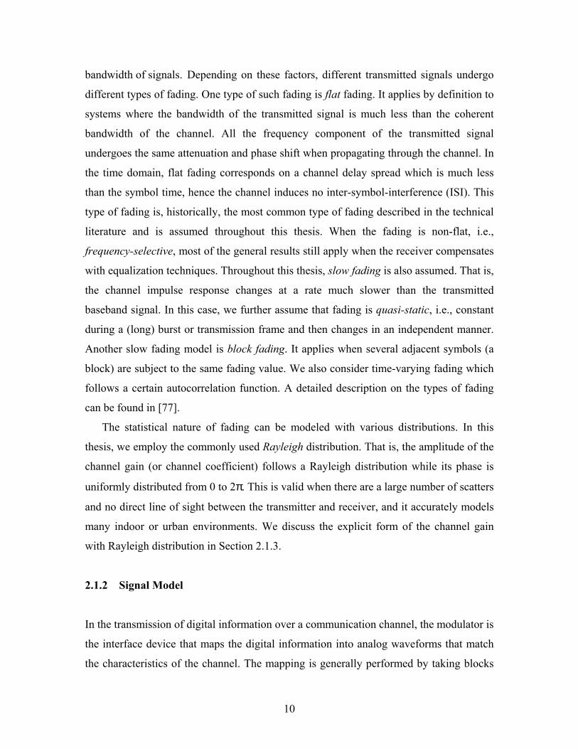
bandwidth of signals. Depending on these factors, different transmitted signals undergo

different types of fading. One type of such fading is flat fading. It applies by definition to

systems where the bandwidth of the transmitted signal is much less than the coherent

bandwidth of the channel. All the frequency component of the transmitted signal

undergoes the same attenuation and phase shift when propagating through the channel. In

the time domain, flat fading corresponds on a channel delay spread which is much less

than the symbol time, hence the channel induces no inter-symbol-interference (ISI). This

type of fading is, historically, the most common type of fading described in the technical

literature and is assumed throughout this thesis. When the fading is non-flat, i.e.,

frequency-selective, most of the general results still apply when the receiver compensates

with equalization techniques. Throughout this thesis, slow fading is also assumed. That is,

the channel impulse response changes at a rate much slower than the transmitted

baseband signal. In this case, we further assume that fading is quasi-static, i.e., constant

during a (long) burst or transmission frame and then changes in an independent manner.

Another slow fading model is block fading. It applies when several adjacent symbols (a

block) are subject to the same fading value. We also consider time-varying fading which

follows a certain autocorrelation function. A detailed description on the types of fading

can be found in [77].

The statistical nature of fading can be modeled with various distributions. In this

thesis, we employ the commonly used Rayleigh distribution. That is, the amplitude of the

channel gain (or channel coefficient) follows a Rayleigh distribution while its phase is

uniformly distributed from 0 to 2π. This is valid when there are a large number of scatters

and no direct line of sight between the transmitter and receiver, and it accurately models

many indoor or urban environments. We discuss the explicit form of the channel gain

with Rayleigh distribution in Section 2.1.3.

2.1.2 Signal Model

In the transmission of digital information over a communication channel, the modulator is

the interface device that maps the digital information into analog waveforms that match

the characteristics of the channel. The mapping is generally performed by taking blocks

10

of k = log2L binary digits at a time from the information sequence and selecting one of L

= 2k deterministic, finite, energy waveforms for transmission over the channel. When

analyzing communication systems, it is often unnecessary to model the up- and down-

conversion between the baseband and the carrier frequency. So, one can choose to work

with baseband models, or equivalent low pass signals and channels, which then become

complex valued. Throughout this thesis, we use complex baseband representation of

signals. The following modulations are considered.

Phase shift keying (PSK): the baseband representation of PSK signals is

PSK = { }1,,1,0,/2 −= Lke Lkj Kπ

The special case when L = 2 is the binary phase shift keying (BPSK). Signal space

diagrams, or signal constellations, for L = 2 and 4, are shown in Fig. 2.1.

0 (0) 1 (1)

0 (00)

1 (01)

2 (11)

3 (10)

Fig. 2.1: BPSK and QPSK constellations

Pulse amplitude modulation (PAM): the baseband representation of this

modulation is

PAM = { } )1(,,3,1 −±±± LK

Quadrature amplitude modulation (QAM): the baseband representation of QAM

signals is

QAM = {a + jb ; a, b∈ {±1, ±3, ± ( − 1)}} 2/1L

Examples of signal constellations are shown in Fig. 2.2 for L = 16 and 32.

Representation of other modulation schemes can be found in [78].

11

12

8

4

0

13

9

5

1

14

10

6

2

15

11

7

3

23

17

11

5

24

18

12

6

25

19

13

7

26

20

14

8

28 29 30 31

0 1 2 3

16

10

4

21

15

9

22 27

Fig. 2.2: 16QAM and 32QAM constellations

2.1.3 MIMO Channel Model

A multi-antenna system is simply an arbitrary wireless communication system in which

the transmitter side as well as the receiver side are equipped with multiple antenna

elements. Fig. 2.3 illustrates the simplified baseband system diagram of a point-to-point

wireless communication link with multiple antennas.

coding

modulation

weighting/mapping

010011

weighting/demapping

demodulation

decoding

010011

N RxM Tx Fig. 2.3: System diagram of MIMO wireless communications.

As can be seen, the underlying nature of using multiple antennas compared with

traditional single-antenna systems is to create a MIMO channel, in which each path from

one transmit (Tx) antenna to one receive (Rx) antenna can be viewed as one signaling

branch. By collecting all of the branches, the MIMO channel can be fully described using

an N × M matrix H, where N is the number of Rx antennas, M is the number of Tx

antennas, and the (n, m)th entry hn,m denotes the channel coefficient from transmit

antenna m to receive antenna n. In general, the correlation between all of the entries in the

12

channel matrix depends on the physical separation of the antenna elements at both sides,

the antenna polarization patterns, the wavelength and the location of surrounding scatters.

In a rich-scattering environment with devices capable of providing enough space to

allocate multiple antennas without coupling, it is usually valid to assume that they are

independent and identically distributed (i.i.d). Hence, based on the considered flat

Rayleigh fading model, the entries can be modeled as samples of independent complex

Gaussian random processes with zero mean and unit variance:

=mnh , Normal (0, 0.5) + ⋅j Normal (0, 0.5).

Consequently, is a chi-square random variable with degree of 2, , but

normalized to = 1.

2, || mnh

|[| 2,mnhE

22χ

]

Let ct denote the M × 1 baseband transmitted signal vector at discrete time slot t, and

rt be the N × 1 baseband received signal vector. As the signal at each Rx antenna is

simply a noisy superposition of the M transmitted signals corrupted by different fading,

the input-output relationship of the MIMO channel is modeled compactly as

ttt wHcr += (2.1)

where wt is a vector of additive white Gaussian noise (AWGN) terms.

2.1.4 Digital Transmission over MIMO Channels

A basic transmission and detection procedure over MIMO channels is described as

follows. Consider the wireless communication link shown in Fig. 2.3. A compressed

digital source in the form of a binary data stream is fed to a transmitting block

encompassing the functions of error control coding and (possibly joined with) mapping to

complex modulation symbols (QAM, PSK, etc.). The latter produces several separate

symbol streams which range from independent, to partially redundant, to fully redundant.

Each is then mapped onto one of the multiple transmit antennas. Mapping may include

linear spatial weighting of the antenna elements or linear space-time precoding. After

upward frequency conversion, filtering and amplification, the signals are launched into

the wireless channel. At the receiver, the signals are captured by multiple antennas and

demodulation and demapping operations are performed to recover the message.

13

In general, the design of above channel coding, modulation and mapping is very

different from that of traditional schemes used in SISO channels. This is mainly due to

the presence of a new signaling dimension: space, inherently brought by multiple

antennas, especially multiple transmit antennas. Hence, the MIMO-related transmission

techniques can be referred to as space-time techniques. The selection of detailed

techniques varies a lot depending on whether one or both sides have knowledge of fading

coefficients, i.e. CSI. Typically, it is very difficult to obtain channel knowledge at the

transmitter side and, hence, transmitter knowledge is not discussed in this thesis. In fact,

receive knowledge is a fairly common assumption and is possible through a training

sequence and/or a separate pilot channel. In mobile environment where the channel

changes rapidly, however, precisely tracking the channel variation is difficult. Moreover,

while a large number of transmit antennas increase the training period, which

significantly reduces the system efficiency, a large number of receive antennas increase

the complexity of channel estimation. Therefore, in our research, both the coherent and

non-coherent cases in which CSI is available and unavailable, respectively, at the receiver

are considered. We review existing transmission schemes in Section 2.3

2.2 Performance Measure

2.2.1 Channel Capacity

Radio spectrum is a very scarce and expensive resource in wireless communications. The

goal has always been to try to transmit as much information as possible over a given

limited spectrum. Channel capacity is the information-theoretic measure of maximum

possible information transfer rate per unit bandwidth (in bit/s/Hz) with reliable

transmission over a channel, subject to specified constraints.

The very famous capacity formula of a MIMO channel given that the channel matrix

H is known to the receiver can be expressed as [1, 2]

+= H

N MC HHI ρ

2log (2.2)

14

where H is the channel matrix and ρ is the total transmitted SNR. This capacity is

achieved when the transmitted signal vector in (2.1) is composed of M statistically

independent equal power components each with a zero-mean Gaussian distribution. The

capacity in (2.2) is, in fact, a random variable because of the randomness of the channel

matrix H. One way to characterize it is to use the average (or ergodic) capacity which is

obtained by taking the average over all H. Let K = min{M, N} and K’ = max{M, N}, then

a lower bound of the average capacity at high SNR can be derived as [1]

[∑+−=

+≥'

1'

2222 loglog

K

KKiicoherent E

MKC χρ ] , (2.3)

where is a chi-square random variable with a degree of 2i. This lower bound is

asymptotically tight at high SNR. It is observed that at high SNR, a 3-dB increase in ρ

yields a K-bit/s/Hz increase on the capacity, in contrast to a 1-bit/s/Hz increase for

traditional single-input single-output (SISO) channels. This result suggests that the

MIMO channel can be viewed as K parallel spatial channels, and that K = min{M, N} is

the total number of degrees of freedom to communicate. Therefore, independent

information symbols can be transmitted in parallel through the spatial channels to

increase the spectral efficiency. This is also called spatial multiplexing in [72].

22iχ

The study of the channel capacity when H is unknown at the receiver is a little bit

more complicated. It was initiated by Marzetta and Hochwald in [51] for block fading

channels with a block length equal to T discrete time intervals. It is shown that for any

fixed N Rx antennas, the capacity obtained with M > T transmit antennas is the same as

the capacity obtained with M = T transmit antennas. Thus, in what follows M ≤ T is

always assumed. Second, the capacity-achieving random signal matrix may be

constructed as a product C = VΦ, where Φ is an M × T istropically distributed matrix

with orthonormal rows and V is an independent M × M real non-negative diagonal

matrix. Notice that this capacity-achieving input distribution is very different from the

Gaussian distribution in the coherent case. The non-coherent channel capacity was further

analyzed by Zheng and Tse in [52] using a geometric approach. It was shown that the

average channel capacity at high SNR is asymptotically equal to

15

aT

MMC coherentnon +

−=− ρ2

** log1 (2.4)

where M* = min{M, N, T/2} and a is some constant independent of ρ. In particular, if M

< N and T ≥ M + N, the degree of freedom for non-coherent communication without

imposing a training sequence is only . ( )TMM /1−

2.2.2 Error Probability and Pair-Wise Error Probability

Although channel capacity can somehow motivate the design of transmitted signals (e.g.

[53] as well as receiver structures (e.g. [1, 3]), the drawback is that it usually does not

reflect the performance achieved by actual transmission systems, since it only provides an

upper bound realized by codes with boundless complexity or latency. In practice, the

probability of error is used to measure the reliability or robustness of a communication

strategy.

Pair-wise error probability (PWEP) between any two possible codewords is defined

as the probability that a certain receiver makes an error in favor of one codeword when

the other is actually transmitted. In fading channels, PWEP reveals the effect of some

dominant factors (e.g., diversity gain and coding gain, see Section 2.2.4) in coded system

performance. And, it usually can be calculated with a closed-form tight upper bound.

Hence, in MIMO systems, the worse case PWEP over all possible distinct codeword pairs

is often used to specify the design criteria for constructing proper coding and/or

modulation.

With PWEP, the bit error probability (BER), symbol error probability (SER), or

frame error probability (FER) can be consequently derived. In general, however, it is

difficult to give an explicit expression for these error probabilities in a system.

Alternatively, computer simulation is usually used. The error probability is obtained by

counting the error numbers with respect to the total number of transmission realizations.

The accuracy of simulation results depends on the number of realizations. Usually, 100

error numbers are required to obtain ± 0.1 accurate results.

16

2.2.3 Diversity

Diversity is a powerful technique in wireless communications used to mitigate random

fading at relatively low cost. The basic idea of diversity is to exploit the random nature of

radio propagation by finding independent (or at least highly uncorrelated) signaling

branches for communication. If one channel branch undergoes severe attenuation, another

independent branch may have a strong signal. A key concept is the diversity order, which

is defined by the number of independent channel branches. The probability of losing the

signal vanishes exponentially with the diversity order. Hence, diversity order is one of the

parameters used to evaluate system error performance in fading channel. A simple

example of diversity technique is channel coding coupled with interleaving.

In a MIMO system with M Tx and N Rx antennas, there are MN independent spatial

channels, through which replicas of the same information data can be transmitted.

Intuitively, the maximum possible antenna diversity order is up to MN.

Of the antenna diversity techniques, receive antenna diversity is already well

developed. It can be achieved using selection diversity (selecting the antenna with the

highest signal power) or maximum-ratio-combing (weighting and combing the received

signals to maximize the SNR) when CSI is available at the receiver. It is, however, not

easy to achieve transmit diversity when the transmitter cannot access CSI. In general,

channel coding (either trellis-based or block-based) should be applied across both the

time domain and space (Tx antennas) domain so as to achieve transmit diversity. This is

the general concept of the so-called space-time coding [8].

2.2.4 Coding Gain

Beside diversity, coding gain is another useful parameter used to measure the error

performance of a system over fading channels. Originally it was used in AWGN

channels as the ratio of the minimum free Euclidean distance of a coded system to the

minimum Euclidean distance of an uncoded system. This value asymptotically reflects

the SNR reduction of a coded system over an uncoded system for achieving the same

17

amount of error probability. This term is now also applied in coded MIMO systems with

fading channels, but may not refer to Euclidean distance.

In [8] coding gain/advantage is defined from the pair-wise error probability as

follows. If the PWEP is upper bound as dSNRPWEP −⋅≤ δ

in the region of high SNR, then the system is said to have diversity advantage of d and

coding advantage of δ. As can be seen, the coding gain in MIMO systems shifts the upper

bound of the PWEP up or down and is the approximate measure of the gain over an

uncoded system operating with the same diversity order. Later on it will be shown that, in

a space-time coded system with diversity advantage of d = MN, the coding gain refers to

the minimum determinant of the Hermitian square of codeword error matrix [8].

2.3 Relevant MIMO Transmission Schemes

In this section we present an overview of relevant MIMO transmission schemes. As can

been seen from Section 2.2, MIMO systems can provide spatial multiplexing gain and

spatial diversity gain. These two types of gains reflect the spectral efficiency of a wireless

link and its reliability, respectively, and they are often mutually conflicting. Most of the

current ST techniques can be, therefore, classified into three categories: rate-oriented,

diversity-oriented, and rate-diversity-oriented.

2.3.1 Rate-Oriented Layered Space-Time Architecture (VBLAST)

The goal of rate-oriented schemes is to increase the spectral efficiency by sending

multiple independent data streams simultaneously on the same frequency band. The

number of independent data streams, or the order of the multiplexing gain, is equal to the

minimum number of transmit and receive antennas, which agrees with the capacity

behavior in (2.3). These schemes usually work when the transmitter and the receiver are

both equipped with multiple antennas.

Among these schemes, layered space-time architecture (LST) is innovative and

practical scheme. It was developed by Bell-Lab [3, 4, 5], and, thus, also known as

18

VBLAST (Vertical Bell-lab LAyered Space-Time architecture). In this scheme, each Tx

antenna simply sends an independent data stream (also called layer) simultaneously with

all of the other antennas on the same frequency band. The detection strategy at the

receiver is somehow motivated by the information-theoretic result in (2.3). Each layer is

regarded as one virtual user and detected successively with certain ordering. To be

specific, when detecting one layer, all of the other not-yet-detected layers are treated as

interference and nulled out based on zero-forcing (ZF) or minimum mean square error

(MMSE) criterion. After this layer is detected, its contribution is subtracted and the

detection jumps to the next layer. What makes the VBLAST scheme famous is, in fact,

the ordering method, the basic idea of which is to select the strongest layer from all the

not-yet-detected candidates to detect at each detection level. It has been proved that this

ordering method can maximize the minimum post-detection SNR over all layers and,

hence, minimize the overall error probability [6]. Obviously, the spectral efficiency in

this scheme increases linearly with the number of Tx antennas, M. However, it should be

noticed that the number of Rx antennas should not be less than that of Tx antennas, N ≥

M, in order to apply the layer-by-layer detection algorithm. In addition, the overall

system performance is dominated by the layer with the worst error probability and, hence,

is usually very poor when N is not large enough, relative to M.

The complexity of VBLAST detection algorithm can be further reduced by a square-

root algorithm [42]. And its performance can be enhanced through the use of outer

channel coding [41] or better decoding algorithms, such as maximum-likelihood (ML)

decoder [377], sphere decoder [67], and iterative algorithm [38, 39, 40]. Notice that the

use of outer channel coding also reduces the spectral efficiency.

2.3.2 Diversity-Oriented Space-Time Codes

Space-time coding (STC), also called space-time coded modulation, is a revolutionary

diversity-oriented development that aims at improving the error probability behavior by

performing coding across time and space (transmit antennas). It works with multiple

transmit antennas and does not necessarily need multiple receive antennas. Delay

diversity transmission, proposed in [43, 44], is probably the first STC scheme. It

19

transmits delayed copies of the same information signal sequence on multiple antennas,

and is seen at the receiver as a single-antenna transmission with increased channel delay

spread. The spatial diversity is, thus, artificially transformed to multipath diversity where

the gain can be realized at the receiver using the Viterbi-algorithm based maximum

likelihood sequence estimator (MLSE) [45]. This transmission scheme can be designed

for an arbitrary number of transmit antennas with arbitrary signal constellations. From a

coding perspective, it can be viewed as a systematic approach of designing ST codes and

is, hence, referred to as the delay diversity (DD) coding. The more general concept of

STC was later introduced by Tarokh et al [8].

Based on code structure, space-time codes can be divided into space-time trellis codes

and space-time block codes (STBC). STTC can be fully specified using a trellis diagram.

At each time t, depending on the state of the ST encoder and the input bits, a transition

branch is chosen. If the label of this branch is , then transmit antenna m is used

to send constellation symbols , m = 1, 2, …, M and all these transmissions are

simultaneous. Presented in Fig. 2.4 is an example of the trellis diagram for the 4-state

QPSK-modulated code using two transmit antennas [8, Fig. 4]. The mapping of the

QPSK constellation symbols is given in Fig. 2.1. At the receiver, a vector-based Viterbi

algorithm is applied to perform ML decoding.

Mttt xxx L21

mtx

30, 31, 32, 33

20, 21, 22, 23

10, 11, 12, 13

00, 01, 02, 03

Fig. 2.4: QPSK 4-state ST code with 2 transmit antennas

Under different channel environments, different criteria are needed for the design of

good space-time codes. In particular, the well-known and fundamental design criteria

over quasi-static flat Rayleigh fading channels are the rank criterion and the determinant

criterion [8, 7]. The rank criterion is used for achieving maximum diversity gain, while

the determinant criterion is for maximizing the coding gain. These two criteria have been

20

widely used to construct many classes of space-time trellis codes. In STTC, to achieve

full transmit diversity, the minimum required number of trellis states grows exponentially

with the number of transmit antennas and the transmission efficiency (in bit/s/Hz). The

result is an exponential increase in the decoding complexity. All the handcrafted space-

time trellis codes using two transmit antennas provided in [8] are full rank, thus attaining

maximum diversity gain, but may not have maximum coding gain. Subsequent computer

searches were carried out in [25, 26, 27, 28] to find codes with higher coding gains. New

code construction methods were also proposed, including the algebraic approach for

BPSK and QPSK modulation [34, 35], the systematic approach [47], generalized delay

diversity coding [46], and our proposed diagonal block space-time (DBST) coding

[Tao3].

Instead of following the traditional design criteria, several investigations were done

by [30, 29], and [Tao2] into different design criteria where, in particular, the role of the

Euclidean distance was studied at low SNR, or equivalently at a large number of receive

antennas. The corresponding codes in [31, 32, 33] and our codes in [Tao2] with a large

minimum Euclidean distance and non-full transmit diversity perform well with enough

receive antennas but poorly when the number of receive antennas is small.

A space-time block code is essentially a linear mapping from a group of modulated

data symbols onto codeword matrices in the space-time grid. There are several types of

STBCs based on the different theories employed in the code construction, such as

orthogonal designs [11, 9], amicable orthogonal designs [12, 13, 15], and algebraic

designs with constellation rotation [70]. The first orthogonal STBC for two antennas was

discovered by Alamouti [11] and, hence, is often referred to as Alamouti’s scheme. In

this scheme, the symbols input to the space-time block encoder are divided into groups of

two symbols each. At a given symbol periods, the two symbols in each group {c1, c2} are

transmitted simultaneously from the two antennas. That is, the signal transmitted from

antenna 1 is c1 and the signal transmitted from antenna 2 is c2. In the next symbol period,

the signal is transmitted from antenna 1 and the signal is transmitted from antenna

2. Hence, the codeword matrix (denoted by G

*2c− *

1c

2) can be written as

−= *12

*21

2 ccccG . (2.5)

21

Assume the channel coefficients keep constant over these two consecutive symbol

periods. Then the two symbols c1, c2 can be decoupled and decoded individually at the

receiver based on simple linear processing, and each of them achieves the transmit

diversity of order 2. This is due to the orthogonality attained in the codeword structure

(2.5). The very simple structure and linear processing of Alamouti’s scheme makes it a

very attractive scheme, and it is currently part of both the W-CDMA and CDMA-2000

standards. This scheme was later generalized by [9] to an arbitrary number of transmit

antennas using the theory of orthogonal designs. Define the code rate as the ratio of the

number of information symbols contained in each codeword to the number of symbol

periods the codeword occupies. It was shown that, for real signal modulation, e.g. PAM,

orthogonal STBC with rate 1 can be constructed while, for general complex modulation

like multi-level QAM and multi-level PSK, a rate-1 orthogonal STBC with simple linear

processing based ML detection and achieving full antenna diversity does not exist for M

> 2. There is a tradeoff among the orthogonality, the rate of the code, and the order of

transmit diversity. For example, the rate ¾ orthogonal code for M = 4 (denoted by H4)

achieving full transmit diversity is given by

−−+−−++−

−−

=

211233

122133

*3

*3

*12

*3

*3

*21

4

2222

2222

jyxjyxccjyxjyxcc

cccccccc

H (2.6)

in which xi and yi are the real part and imaginary part of the complex symbol ci

respectively. The design of quasi-orthogonal codes can be found in [14, 16, 17, 18], some

of which may sacrifice the diversity gain to have a higher code rate. The diagonal

algebraic STBC proposed in [70] solves this problem. It achieves full transmit diversity at

rate 1. However, it creates new issues as well, e.g. peak-to-average power ratio and

receiver complexity.

In general, STBC performs worse than STTC due to lower coding advantage. Some

efforts have been made in [20, 21, 22, 23, 24] on the concatenation of orthogonal STBC

and outer channel coding in order to enhance the coding advantage.

22

2.3.3 Rate-Diversity-Oriented Space-Time Techniques

There are two types of rate-diversity-oriented space-time techniques. One achieves both

diversity gain and multiplexing gain, and ensures a balance between the two, while the

other, more ambitious, endeavors to achieve full diversity gain and maximum

multiplexing gain simultaneously. Examples of the former technique, found in [19, 40],

can be viewed as a direct compromise between diversity-oriented space-time codes

(STTC or STBC) and rate-oriented VBLAST. The study on this rate-diversity tradeoff

technique was then intensively conducted in [Tao4]. Examples without a tradeoff include

the linear dispersion codes [68, 69], the threaded algebraic space-time codes [73], and the

algebraic code for two transmit antennas [71]. All these codes apply (linear) precoding at

the transmitter and use sphere decoder [66] at the receiver to do ML decoding. The

disadvantage of these codes compared with the tradeoff-type scheme is the expansion of

transmitted signal points due to the use of complex-field precoding. So far, there has been

only limited work on this non-tradeoff topic.

2.3.4 Non-Coherent Diversity-Oriented (Differential) Unitary Space-Time

Modulation

The information-theoretic study in [51] suggests a capacity-achieving signal structure

which comprises complex-valued signals that are orthonormal with respect to time among

the transmit antennas. Specifically, the M × T transmitted signal matrix on M antennas

over T time intervals has the partitioned form , where the M

rows, representing the temporal signals fed to the M Tx antennas, are mutually

orthogonal. It is further shown that setting v

[ ]TTMM

TT vvv φφφ ,,, 2211 K=C

1 = v2 = … = vM = T achieves capacity for

either T >> M or for high SNR and T > M. Unitary space-time modulation (USTM) [53]

is, hence, defined as the transmission of ΦT=C , where . I=HΦΦ

To design a USTM with good error performance, one should follow the criterion: for

any pair of codewords C1 and C2, none of the singular values of Φ should be 1. In

other words, C

H21Φ

1 and C2 should be made as orthogonal as possible. In this case, the

23

number of singular values that are not equal to 1 quantifies the order of achieved transmit

diversity. Several examples are provided in [53] and [54].

Most of current USTM schemes were designed with T = 2M, and are somehow not

very spectrally efficient. A differential USTM was then proposed in [56 57， ]. There can

be two different ways to look at DUSTM. First, it can be regarded as an overlapped

USTM with T = 2M, in which the first half of a USTM signal matrix is made the same as

the second half of a previously transmitted signal matrix by a certain information-lossless

unitary transformation. Therefore, when transmitting this signal matrix, it is only

necessary to send the second half. Also, DUSTM can be viewed as an extension of the

traditional differential PSK modulation used in single-antenna systems. The main

difference is that the signal constellation is no longer the set of scalar symbols with unit

amplitude, but the set of M × M complex-valued unitary matrices.

The encoding processing of DUSTM is briefly reviewed. As the signals are

transmitted in the unit of block, each containing M time intervals, it is convenient to use k

= 0, 1, … to denote the block index; within the kth block, the time index is denoted as t =

kM, kM + 1, …, kM + M − 1. We let Ck denote the M × M unitary signal matrix

transmitted over M transmit antennas during the kth block. The differential transmission is

initiated by sending the identity matrix, i.e. C0 = IM. Then, with differential encoding, we

have, at block k = 1, 2, …,

)(1 klkk VCC −= , (2.7)

where Vl(k), with l(k) ∈ {0, 1, …, L−1}, is the M × M data matrix at time block k and is

selected from a unitary matrix constellation V with size L, i.e. Vl(k) ∈ V ≡ {Vl | VlH

lV = I,

l = 0,1,…, L−1}. The transmitted signal matrix Ck generally does not belong to the

constellation unless the constellation itself forms a group under matrix multiplication.

The design of signals constellations follows a similar rank and determinant criteria.

Existing constellations for DUSTM include the diagonal cyclic group constellations

discussed in [57], group constellation of [56], Alamouti’s scheme in [44, 63], our

proposed orthogonal STBC [Tao7], amicable orthogonal codes [59], parametric codes

[62], and other group and non-group constellations [55]. For a large number of receive

antennas, diagonal cyclic group codes were presented in [61].

24

Chapter 3

IMPROVED DESIGN OF SPACE-TIME TRELLIS

CODES AT DIFFERENT SNR

In Chapter 2, we reviewed the concept and several key design examples of space-time

coding. It is known that the traditional rank and determinant criteria been widely used to

construct many classes of space-time trellis codes. Several handcrafted space-time trellis

codes using two transmit antennas were provided in [8]. These codes are full rank but

may not achieve the maximum coding gain. Subsequent computer searches were carried

out in [25, 26] to find codes with larger coding gain. However, it is worth to notice that

the derivation of traditional rank and determinant criteria was based on the assumption

that the SNR is sufficiently high. From existing simulation results [8, 25, 26], we observe

that to achieve a frame error rate (FER) of 10-2, the codes with QPSK modulation and 2

bit/s/Hz transmission efficiency require only around 10 dB transmit SNR when the

number of receive antennas, N, is equal to the number of transmit antennas, M (M = N = 2

in this example). Even smaller SNR is required when N > M. In this situation, the

assumption of high SNR is not valid and thus the two criteria are not tight.

In this chapter, we address the issue of non-high SNR and derive more precise criteria

for designing space-time trellis codes. Based on our new criteria, we also provide several

code examples using computer search. The remainder of this chapter is organized as

follows. We start by introducing the system model in Section 3.1. In Section 3.2, we

derive the improved design criteria. The trellis code examples and their simulation results

are provided in Section 3.3. Finally Section 3.4 summarizes this Chapter. The results in

this chapter are published in [Tao2].

25

3.1 System Model

We consider a point-to-point wireless link with M transmit antennas and N receive

antennas as shown in Fig. 2.3. It is assumed that the channel is quasi-static flat Rayleigh

fading and the channel coefficients are perfectly known to the receiver. The received

signal on antenna n at time slot t is given by

nt

mt

M

mmns

nt wchEr += ∑

=1, (3.1)

where hn,m is the normalized channel coefficient from transmit antenna m to receive

antenna n; c is transmitted symbol by antenna m at time t and chosen from a certain

constellation (e.g. PSK and QAM) with unit average energy; is the additive complex

white Gaussian noise with zero mean and variance ; and E

mt

ntw

0N s is the average energy per

symbol. The SNR is defined to be total transmitted signal energy to noise power spectral

density ratio, and given by 0NMEs=ρ .

3.2 Improved Design Criteria

A space-time codeword is defined as an M × T matrix, with T being the codeword length

=

MT

MM

T

T

ccc

cccccc

L

MOMM

L

L

21

222

21

112

11

C (3.2)

in which the t-th column represents the space-time symbol transmitted at time t and the

m-th row be the symbol sequence transmitted from antenna m. Suppose C, E ∈ are

two possible space-time codewords. Let B be the codeword error matrix defined by

. Further define A = BB

TM ×C

ECB −= H, in which the (p, q)-th entry can be written as

[ ] ( )( *

1,

pt

pt

T

t

pt

ptqp ecec −−=∑

=A ) . (3.3)

The Chernoff bound of the pair-wise error probability (PWEP) has been derived in [8] as

26

( ) ( )[ NM

NM

iiM

P −−

=+=

+≤→ ∏ AIEC αλρ det

41

1] (3.4)

where α = M4ρ , and λi, i = 1, 2, …, M, are the eigenvalues of A with λ1 ≥ λ2 ≥ …λn ≥

0. Evidently, to minimize the PWEP, the optimal design criterion is to maximize

( AI )α+det over all C . Unlike [8] where high SNR was assumed, we study the

design criteria for different ranges of SNR. In practical system design, the FER is

required to meet the system specification. Based on the number of transmit and receive

antennas, this FER requirement translates to a minimum required value for α. Given the

FER requirement, the number of antennas and the code complexity, α falls into a certain

range and the objective of code design is to minimize the FER for that SNR range. The

designed code need not be optimal for a higher SNR range as the FER at that higher SNR

range is much better than the requirement already. Similarly, code that works better at a

lower SNR range will not be useful because the FER cannot meet the minimum system

specification anyway. In this contribution, we consider the following three SNR ranges.

E≠

3.2.1 Case 1: α ≈ 1 (Moderate SNR)

As discussed above, the required SNR to achieve 10-2 FER is around 10 dB when M = N

= 2, which results in α=10/(4⋅2)≈1. In general, it is valid to assume moderate SNR for

achieving a FER of most interest when M ≈ N, which implies α ≈ 1. Hence from (3.3) we

reach the following criterion when α ≈ 1:

The minimum determinant of the matrix I + A over all possible distinct codword

pairs C and E must be maximized to minimize the PWEP for moderate SNR.

3.2.2 Case 2: α << 1 (Low SNR)

To see how this assumption can be valid, we observe that, to achieve a target FER, the

required SNR decreases as the number of receive antennas increases. As a result, when N

>> M, α will be much less than 1. Based on this assumption, we ignore the high order

terms of α and further upper bound the PWEP tightly by

27

. (3.5) ( )NM

iiP

−

=

+≤→ ∑

11 λαEC

Since the sum of the eigenvalues is equal to the trace, and the trace of A is exactly the

squared Euclidean distance between the codewords C and E by observing the definition

of A in (3.3), we reach the following conclusion:

The design criteion for low SNR is just to maximize the minimum squared Euclidean

distance of the space-time code.

The role of the squared Euclidean distance in the design of space-time codes was also

analyzed in [23]. The difference is that the problem considered in [23] still assumed high

SNR and a criterion of equating the eigenvalues of A for all pairs of C and E was

reached.

3.2.3 Case 3: α >> 1 (High SNR)

If N << M, we need a high SNR to achieve a desired FER and this is the case most

commonly assumed. The PWEP is now upper bounded by

( )Nr

ii

rNP−

=

−

≤→ ∏

1λαEC (3.6)

where r is the rank of B. Therefore, this reduces to the same criteria as in [7, 8] for high

SNR:

1) Rank Criterion: In order to achieve the maximum diversity MN, the matrix B has

to be full rank for any two distinct codewords C and E.

2) Determinant Criterion: If a diversity of MN is the target, then the minimum

determinant of A which corresponds to coding gain must be maximized.

Note that, except in case 3, the code optimized for case 1 or 2 need not be full rank,

contrary to the common belief that full rank is always needed for good code.

3.3 Computer Searched Trellis Codes for Moderate SNR

In the literatures, there have been several trellis codes designed for space-time coding.

The original one is the handcrafted code in [8] (TSC codes). All of them are full rank in

28

spatial domain. The others are the systematic global searched codes in [14] (BBH codes)

and [15](YB codes). They are also full rank and try to achieve the coding gain as much as

possible by maximizing the minimum determinant of A. In other words, they are all

designed for case 3 and may not be optimal in case 1 and case 2. In this work, we are

more interested in case 1 and consider designing space-time trellis codes for two transmit

antennas functioning optimally at moderate SNR. Hence our searching program will seek

the codes that have the largest minimum determinant of the matrix I + A over all distinct

codeword pairs C and E.

3.3.1 Code Examples

Following both [25] and [26], we use a generator matrix G to represent a space-time

code. We take the space-time code for 2 bit/s/Hz with QPSK modulation and 8 trellis

states in [8, Fig. 5] as an example. Let (at , bt) be the sequence of binary inputs at time t,

the output signal pair 1 2( , )t tx x is given by

( ) ( ) 4mod, 21121 G⋅= −−− ttttttt ababaxx ( )

where

=

2202012010

G .

Tables 3.1 to 3.4 list some of the search results. Three parameters, the minimum

squared Euclidean distance ( ), the minimum determinant of A (det(A)), and the

minimum determinant of I + A (det(I +A)), are given for numerical comparison with the

TSC, BBH and YB codes.

2mind

For the QPSK, 4-state, 2 bit/s/Hz code in Table 3.1, there are many different codes

found by global search that satisfy det(I+A) = 17 but have different and det(A).

Among them, we select the one with the largest d as our new code. We can see that

this new code has the largest out of all the codes listed in this table, the same

det(I+A) as the YB code and smaller det(A) than both the BBH and YB codes. For the Q-

2mind

2min

2mind

29

PSK, 8-state, 2 bit/s/Hz code in Table 3.2, there are also many codes satisfying the same

three parameters. We just randomly pick one as our new code. The new code has the

largest d and det(I+A), but smaller det(A) than the YB code. For the Q-PSK, 16-state,

2 bit/s/Hz code in Table 3.3, we also find multiple codes satisfying det(I+A) = 45. All of

them have the same but different det(A), which is either 28 or 32. We randomly

select one as our new code from those with det(A) = 32. It is seen that the YB code and

our new code have the same three parameters although the generator matrices are

different.

2min

2mind

2min

)A

)A+

The 8PSK, 8-state, 3 bit/s/Hz codes are listed in Table 3.4. No BBH and YB codes

are available in this case. For our new code, the last row of the generator matrix G can be

any permutation of 6 and 2 since they are symmetric in the 8-PSK constellation. We

claim that this is the best code [maximizing det(I+A)] we have found so far. It may not be

the optimal one over global search. As seen in the table, the new code is not full rank as

det(A) = 0, but has larger and det(I+A) than the TSC code. 2mind

Table 3.1: Space-time codes with QPSK, 4 states, 2 bit/s/Hz

G

New

02211220

TSC

01021020

BBH

13012022

YB

12212022

d 10 4 6 8

det( 4 4 8 8

det(I 17 9 15 17

30


G

New

2022112032

TSC

2202012010

BBH

2202012210

YB

2220011220

2mind 12 8 8 10

)det(A 12 12 12 16

)det( AI + 29 25 21 27


G

New

220201102022

TSC

022021021020

BBH

022021021220

YB

200221112220

2mind 12 8 12 12

)det(A 32 12 20 32

)det( AI + 45 21 37 45

Table 3.4: Space-time codes with 8PSK, 8 states, 3 bit/s/Hz

G

New

)2(6)2(64404040120

TSC

050204102040

2mind 6 4

)det(A 0 2

)det( AI + 9.929 7

31

3.3.2 Simulation Results

The simulation results for the QPSK, 8-state, 2 bit/s/Hz code and the 8PSK, 8-state, 3

bit/s/Hz code are of interest since our new codes have the largest det(I+A) in these two

cases. We illustrate the FER performance of these two cases in Fig. 3.1 and Fig. 3.2,

respectively, with two, three and four Rx antennas. Each frame contains 130 transmitted

symbols out of each transmit antenna. The channel coefficients are kept constant within

one frame and changed randomly from one frame to the other frame. From Fig. 3.1 it is

observed that the new code is 0.5~0.8 dB better than the TSC code and slightly better

than the YB code in systems with three and four receive antennas. From Fig. 3.2 it is seen

that the new code performs slightly worse that TSC code at high SNR with two Rx

antennas, but much better with three and four Rx antennas and the gains are 0.8 dB and

1.0 dB, respectively, at a FER of 10-2.

0 2 4 6 8 10 12 1410

−3

10−2

10−1

100

SNR [dB]

Fra

me

Err

or P

roba

bilit

y

2 Rx3 Rx4 Rx

TSCYBNew

Fig. 3.1: Performance of the QPSK, 8-state, 2 bit/s/Hz space-time codes with 2 transmit and 2, 3,4

receive antennas

32

4 6 8 10 12 14 16 1810

−3

10−2

10−1

100

SNR [dB]

Fra

me

Err

or P

roba

bilit

y

2 Rx3 Rx4 Rx

TSCNew

Fig. 3.2: Performance of the 8-PSK, 8-state, 3 bit/s/Hz space-time codes with 2 transmit and 2, 3,

4 receive antennas

3.4 Summary

In this chapter we considered the design of space-time codes in practical systems at

different SNR regions or, equivalently, at different number combinations between

transmit antennas and receive antennas. We derived tighter design criteria than the

traditional ones for low and moderate SNRs. In particular, we showed that the traditional

full-rank criterion is not always necessary. Moreover, the minimum Euclidean distance is

the dominating factor at low SNR in the design of space-time codes minimizing the error

probability. We also provided several new trellis code examples for moderate SNR

33

through computer search. These codes showed better performance than existing codes

under a wide range of low to moderately high SNR conditions.

34

Chapter 4

DIAGONAL BLOCK SPACE-TIME CODING

In the last chapter we discussed the improved design criteria of space-time trellis codes

and also provided several code examples for moderate SNR via exhaustive search. In this

chapter, we are interested in the design of space-time trellis codes when the number of

receive antennas is limited so that the rank and determinant criteria for high SNR are still

valid.

A large number of existing space-time trellis codes are found based on exhaustive

search. Hence they are limited to a small number of transmit antennas (2 or 3) and low-

level modulation (BPSK or QPSK) due to the extraordinary time complexity of

searching. In this chapter, we propose an efficient systematic coding approach that is

suitable for an arbitrary number of transmit antennas with arbitrary signal constellations.

The key of this approach is to separate the traditional space-time code design into two

parts. It first encodes the information symbols by a one-dimensional (M, 1) nonbinary

block code, with M being the number of transmit antennas, and then transmits the coded

symbols through the M antennas in a diagonal pattern. Hence, we refer to this scheme as

diagonal block space-time (DBST) coding. We show that, regardless of the channel time-

selectivity, this new class of space-time codes always achieves a transmit diversity of

order M with the minimum number of trellis states and a coding advantage equal to the

minimum product distance of the employed block codes. Traditional delay diversity

codes can be viewed as a special example in this category where a repetition block code

is employed. To maximize the coding advantage, we introduce an optimal construction of

the nonbinary block code for given modulation schemes. We also propose an efficient

suboptimal solution for multi-level PSK modulation.

Similar work on generalized delay diversity codes was done in [46], where only the

quasi-static fading was considered and it is not clear how to apply its design method to

high-level modulation. A recent work in [47] suggested another systematic design of

space-time trellis codes for quasi-static fading by manually assigning the channel output

35

symbols for each trellis state transition with certain rules. This scheme can achieve the

maximum possible antenna diversity order but its coding advantage is less efficient, as

will be shown in detail. An algebraic approach was presented in [34, 35], but it is only for

BPSK and QPSK modulation.

This chapter is organized as follows. In Section 4.1, we review the system model and

the fundamental performance criteria of space-time codes at both quasi-static and fast

fading channels. The proposed diagonal block space-time code structure and its pair-wise

error probability are described in Section 4.2. The nonbinary block code construction is

presented in Section 4.3, along with some code examples. In Section 4.4, the performance

of the proposed codes is evaluated and compared with that of existing codes. Finally,

Section 4.5 concludes this chapter. The results in this chapter are published in [Tao3,

Tao5]

4.1 System Model and Performance Criteria

The system model considered in this chapter is the same as Chapter 3, except that a fast

fading channel model is included here. While the channel coefficients keep unchanged

within a space-time codeword length in quasi-static fading channels, they vary

independently at different time slots in rapid fading channels.

The pair-wise error probability of mistaking codeword E for C with ML decoder at

both quasi-static fading and rapid fading channels for high SNR can be summarized as

( ) ( ) NP

NE

EM

PH

−⋅−

≤→

4ρEC , (4.1)

in which

(a) Quasi-static fading: EH is the rank of the codeword error matrix B = C−E, and EP

is the product of nonzero eigenvalues of matrix A = BBH

(b) Rapid fading: EH is the size of the time index set of 1 ≤ t ≤ T with c , denoted

by ζ, where c

tt e≠

t (et) is the t-th column in the M × T codeword matrix C (E); and EP

is the product of 2tt ec − over ζ∈t .

36

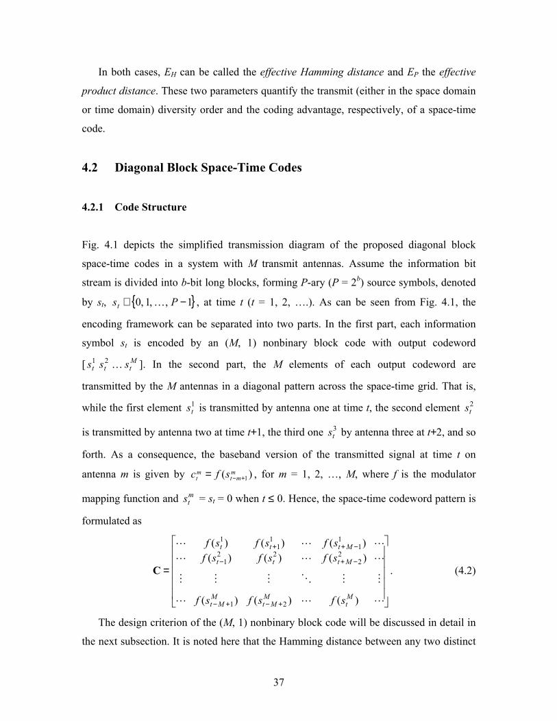
In both cases, EH can be called the effective Hamming distance and EP the effective

product distance. These two parameters quantify the transmit (either in the space domain

or time domain) diversity order and the coding advantage, respectively, of a space-time

code.

4.2 Diagonal Block Space-Time Codes

4.2.1 Code Structure

Fig. 4.1 depicts the simplified transmission diagram of the proposed diagonal block

space-time codes in a system with M transmit antennas. Assume the information bit

stream is divided into b-bit long blocks, forming P-ary (P = 2b) source symbols, denoted

by st, , at time t (t = 1, 2, ….). As can be seen from Fig. 4.1, the

encoding framework can be separated into two parts. In the first part, each information

symbol s

{ 1,,1,0 −∈ Pst K

MtsK

1ts

tc

mts

}

t is encoded by an (M, 1) nonbinary block code with output codeword

[ ]. In the second part, the M elements of each output codeword are

transmitted by the M antennas in a diagonal pattern across the space-time grid. That is,

while the first element is transmitted by antenna one at time t, the second element

is transmitted by antenna two at time t+1, the third one by antenna three at t+2, and so

forth. As a consequence, the baseband version of the transmitted signal at time t on

antenna m is given by , for m = 1, 2, …, M, where f is the modulator

mapping function and = s

tt ss 21

2ts

3ts

)( 1m

mtm sf +−=

t = 0 when t ≤ 0. Hence, the space-time codeword pattern is

formulated as

=

+−+−

−+−

−++

LLL

MMOMMM

LLL

LLL

)()()(

)()()()()()(

21

22

221

11

11

1

Mt

MMt

MMt

Mttt

Mttt

sfsfsf

sfsfsfsfsfsf

C . (4.2)

The design criterion of the (M, 1) nonbinary block code will be discussed in detail in

the next subsection. It is noted here that the Hamming distance between any two distinct

37

block code outputs is equal to M, i.e., there is a one-to-one mapping from each input

symbol to every element in the output codeword [32]. The original delay diversity code

falls in the special case when this block code is a repetition code, i.e., = smts t for all =

1, 2, …, M.

m

(M, 1) Nonbinary Block Code

D

Tx 1

Tx 2

Tx M

st

1ts

D D

Mapper

Mapper

Mapper

2ts

Mts

Fig. 4.1: Transmitter diagram of the diagonal block space-time codes, “D” denotes one symbol

delay

Note that the signal vector ct transmitted at a given time t is governed by the current

input st and the M−1 most recent inputs st−1, st−2, …, and st−Μ+1. The encoder thus forms a

finite-state-machine and we can define the trellis state at time t as

( )121 ,,, +−−−= Mtttt sssS K .

Given that the information symbols are P-ary, the total number of trellis states is equal to

PM−1, which is the minimum number of states for a space-time trellis code to achieve full

antenna diversity over a quasi-static fading channel [8]. During the transition from state St

to state St+1 produced by input st, the encoder outputs M channel symbol indices [

… ], one for each transmit antenna. This procedure can be illustrated as

1ts 2

1−ts

MMts 1+−

( )1

12

11

+ → +−−t

sssst SS

MMtttt K .

Therefore, the Viterbi algorithm can be applied at the receiver to do ML decoding.

4.2.2 Performance Measure

Proposition: In both quasi-static fading and rapid fading channels, the diagonal block

space-time code with M transmit antennas satisfies

MEH =min (4.3)

38

and

∏=−≤<≤

−=M

m

mm

PssP sfsfE1

2

1~0min )~()(min , (4.4)

where EHmin and EPmin are the minimum effective Hamming distance and the associated

minimum effective product distance in the PWEP formula (4.1), [s1 … sM] and

]~~[ 1 Mss K are the two block code outputs generated by inputs s and s~ , respectively.

Note from this Proposition that the proposed DBST codes can always achieve a

transmit diversity of order M, and its coding advantage is governed by the minimum

product distance (PDmin) of the employed (M, 1) nonbinary block code over a chosen

modulation scheme.

Proof: Consider an error event in the Viterbi-algorithm based ML decoder. The

correct and estimated trellis states are denoted by St and tS~ , respectively. Similarly, the

transmitted information symbol sequence and the estimated sequence are denoted by s =

{st} and }~{~ts=s , respectively. Suppose without loss of generality that, in this error

event, the estimated path through the trellis diverges from the correct path at time k and

remerges with the correct path at time k+T. Then, we have

=

−=≠

≠=

++

++

TkTk

tktk

kkkk

SS

TtSS

ssSS

~1,,1for,~

~and~

K . (4.5)

Because every single error in the information symbol sequence propagates M time

intervals by the nature of diagonal transmission, it follows that T ≥ M. The corresponding

space-time codeword difference matrix within this time period is of the form

TMM

MTMM

MT

MT

×−

−

−

∆∆∆

∆∆∆

∆∆∆

=−=

LL

MOOM

L

LL

10

222

20

111

10

00

0 0

00

ECB (4.6)

where )~()( mik

mik

mi sfsf ++ −=∆ , for m = 1, 2, …, M and i = 0, 1, …, T − M.

(a) In quasi-static fading: Partition the codeword difference matrix (4.6) into B = [U

R], where U is an M × M upper triangular matrix and R is an M × (T−M) matrix. Since

39

the inequality s kk s~≠ results in for all m = 1, 2, …, M, U is a full rank matrix.

Then B is also a full rank matrix. Hence the effective Hamming distance E

00 ≠∆m

H is equal to

M. It also yields

( ) ( )( ) ∏

=∆==≥

+==M

m

mH

HHHPE

1

20

2)det(det

detdet

UUU

RRUUBB , (4.7)

where “≥” holds directly from the Minkowski’s determinant inequality [74] as a

Hermitian matrix of the form RRH is nonnegative definite. The equality in (4.7), indeed,

holds if and only if R = 0, i.e., the sequence pair s and s~ are different at time k only. In

the sequel, the final expression in (4.7) corresponds to the product distance between the

two block code outputs [ … ] and [1ks M

ks 1~ks … M

ks~ ] generated by input sk and ks~ ,

respectively. Thus, the results for the quasi-static fading case are proved.

(b) In rapid fading: By definition, EH is now equal to the number of nonzero columns

in B shown in (4.6) associated with the sequence pair s and s~ . It is observed based on

(4.5) that EH = T. Therefore, we have EHmin = M as T ≥ M. Indeed, the minimum occurs if

and only if s and s~ are distinct at time k only. Under this circumstance, the effective

product distance EP is equal to

∏=

∆=M

m

mPE

1

20 . (4.8)

The results in rapid fading are also proved. ■

As in the proof, EH of a DBST code in quasi-static fading channels is always equal to

M for any distinct information sequences s and s~ , but EPmin is obtained if and only if

there is only one symbol error between s and s~ . While, in rapid fading channels, EH

depends on the error sequence and it can be greater than M. Nevertheless, EHmin is still

equal to M and it occurs if and only if there is only one symbol error between s and s~

too. This is because eventually there is no outer coding across the information symbols.

The quasi-static fading and the rapid fading are just the two extreme cases of a general

time-varying fading model. It is, therefore, reasonable to expect that, regardless of the

channel time-selectivity, a DBST code always achieves the diversity advantage and

coding advantage as shown in (4.3) and (4.4), respectively. Simulation results in Section

40

V will demonstrate this statement.

With this Proposition, the optimization of a DBST code simply amounts to finding

the optimal block code that maximizes the minimum product distance given in (4.4). In

particular, the minimum product distance of a repetition code is given by PDmin (rep) =

d2M, where d is the minimum Euclidean distance of the signal constellation. Later on, to

characterize the theoretical performance of our proposed coding scheme, we will treat

delay diversity codes as references and define the asymptotic improvement of a DBST

code as

]dB[rep)(

)new(log10

min

min10 PD

PDM

≡∆∞ . (4.9)

4.2.3 Discussions on Diagonal Structure

The diagonal transmission pattern in the proposed DBST coding has been frequently

utilized in the literature for MIMO systems. It first appeared in [3] as the diagonally

layered space-time architecture (D-BLAST). Recent work includes the trellis coded D-

BLAST [48] and wrapped space-time coding [49]. Most of existing work, designed for

the case when the number of receive antennas N ≥ M, relies on the diagonal structure to

perform a simple ZF or MMSE decision-feedback detection coupled with constituent

decoder at the receiver. This work, instead, applies the diagonal structure to achieve full

transmit diversity, which is essential for reliable transmissions when N < M. In the

sequel, our scheme achieves far lower error probability than the variants of D-BLAST

when N takes a small value (In particular, N = 1 in the downlink of most personal

wireless communication systems).

As another merit of the diagonal transmission pattern in this work, the proposed

DBST coding scheme can be easily extended to frequency-selective fading channels. As

done in [50] for delay diversity codes, we can change the delay step in Fig. 4.1 from one

symbol period to L symbol periods, with L being the number of channel taps. Therefore,

the maximum possible combined transmit diversity of order LM is achieved, as shown in

[50].

41

4.3 (M, 1) Nonbinary Block Code Construction

In the last section we introduced the DBST code structure and derived the minimum

product distance criterion (4.4) for designing the employed (M, 1) nonbinary block code

with M transmit antennas. In this section we discuss the construction of this 1-D code in

detail.

4.3.1 Optimal Construction for Given Constellations

We first consider the optimal code construction. Let c , which is the m-th

element in the block code output corresponding to input s∈ , with m = 1, 2,

…, M. Due to the one-to-one mapping between s and every , the P-long sequence

, , …, forms a permutation of the numbers 0, 1, …, P−1. The

ultimate code design is, therefore, to find these permutations for m = 1, 2, …, M that give

the largest minimum product distance over a given modulator mapping function. As the

numbers 0, 1, …, P−1 can be arranged in P! different ways, the size of the exhaustive

search space is . As each transmit antenna is statistically equivalent to every other

in the space domain, the permutation on the first antenna can be fixed. Without loss of

generality, we simply let it be the natural order {0, 1, …, P−1} and form a systematic

block code with . For constellations in symmetrical shape, the size can be further

reduced, as done for QPSK modulation in [46]. Yet, as the increase of P and M, the

complexity of exhaustive search still increases prohibitively.

mm ss =)(

,,1,0{ PK

)(scm

}1−

)0(mc )1(mc )1( −Pcm

M

s=

( )P!

s1

To solve this permutation optimization problem efficiently, the general branch and

bound algorithm [75] can be applied. The thrust of this algorithm is to form a tree

structure (branching operation) and establish a lower bound (bounding operation). We

take M = 2 for example to illustrate its application in our problem. As discussed above,

our problem is to find the permutation on the second antenna that can give the largest

minimum product distance. In the first level of the tree, the root has P children each

denoting an integer number between [0, P-1]. Each node in the first level further has P-1

children, each denoting an integer selected from [0, P-1]. During the construction of the

42

tree, a child node must be distinct from its ancestor nodes. The tree has P levels. Each

path from the root to a leaf corresponds to a possible permutation, while the whole tree

enumerates all P! permutations. The algorithm then traverses the tree in the depth-first

manner. When reaching a node of the tree, a local minimum product distance is

calculated. If it is greater than a given lower bound of the largest minimum product

distance, the search continues. Otherwise, the remaining tree associated with this node is

pruned. Once a permutation is found, it is used to form or improve the lower bound of the

largest minimum product distance. The extension to M > 2 is straightforward. The height

of the tree is still P. But the number of nodes in each level grows exponentially with M.

Table 4.1 and 4.2 list some of search results. Notice that the solution for P = 2 with

BPSK modulation at any M is just the repetition code and no more gain can be obtained

using other permutations. The modulator mapping function for P-ary PSK modulation is

given by f(s) = , while the mapping for QAM modulation with P = 16 and 32 is

shown in Fig. 2.2. For each code, all the codewords are arranged in an M × P matrix,

where each M × 1 column vector represents one codeword and P is the total number of

codewords. To illustrate the mapping of the nonbinary block codes onto the proposed

DBST codes, Fig. 4.3 gives an example of the trellis diagram for P = 4 (QPSK) and M =

2, in which the branch label xy denotes the symbols on antenna 1 and 2 respectively.

( Psie /2π )

Table 4.1 and 4.2 also shows the asymptotic improvement ∆∞, defined in (4.9), for

comparison. In particular, the ∆∞’s of the QAM codes in Table 4.2 are over the PSK

repetition codes. As we can see, although no improvement can be obtained in terms of

PDmin, the QPSK code with M = 2 has less multiplicity (multi = 2) than the repetition

code (multi = 4).

Notice that the optimal code for each pair of P and M listed in these two tables is not

unique due to the symmetric constellations. As a result, the 8PSK code with M = 2 is the

same as the 8PSK 8-state code designed by Tarokh et al for two transmit antennas in [8].

43

Table 4.1: Optimum block codes used in DBST coding for P = 4 and 8 with PSK modulation

P M Codeset PDmin(new) PDmin(rep) ∆∞ [dB]

2

23103210 4 (multi=2) 4(multi=4) 0

3 ref. [46]

312023103210

16 8 1.00

4 ref. [47]

3120231032103210

32 16 0.75

5

31202310231032103210

64 32 0.60

4

6 ref. [47]

312031202310231032103210

256 64 1.00

2

5274163076543210 ref. [8] 2 0.3431 3.83

3

526147304613752076543210

4 0.2010 4.33

4

36157240623751405267431076543210

4.6863 0.1177 4.00

5

5472163016472530475261305276341076543210

13.6569 0.0690 4.59

8

6

631572404516273051472630743165203745621076543210

32 0.0404 4.83

44

Table 4.2: Optimum block codes used in DBST coding for P =16 and 32 with PSK/QAM

modulation

P M Codeset PDmin(new) ∆∞ [dB] 2

PSK

81331015612194147211501514131211109876543210 0.4210 6.30

2 QAM

53814121017241591113601514131211109876543210 0.64 7.21

3 PSK

49142115158121610313707133106112815511214940

1514131211109876543210 0.8929 8.01

3 QAM

11071251492834156131014613101211072514915831

1514131211109876543210 1.28 8.53

16

4 PSK

12269133158410141511707101123613815294111450

12610151511841429137301514131211109876543210

2 8.93

2 PSK

162772121429924419311226617122102815320825133018523110

313029282726252423222120191817161514131211109876543210

L

L

0.1196 9.54

32

2 QAM

162118141229731282526152211962353027242019817131021430

313029282726252423222120191817161514131211109876543210

L

L

0.2 10.66

02, 12, 22, 32

03, 13, 23, 33

01, 11, 21, 31

00, 10, 20, 30

Fig. 4.2: Trellis diagram for the DBST code with QPSK and M = 2.

45

4.3.2 Linear construction for PSK modulation

The branch-and-bound algorithm can usually reduce the time of searching optimal codes.

However, as the search space grows exponentially, the searching time could still be

dramatically long for large P and M and renders this algorithm impractical. Hence, we

propose an efficient approach which may produce suboptimal solutions. This approach is

particularly applied for PSK modulation. By observing that the signal points in a P-ary

PSK constellation are evenly distributed on a unit circle, we can construct a linear block

code over a ring of integers, denoted by ZP = {0, 1, …, P−1}. The mapping from the ring

ZP onto the constellation is given by , for . Let the generator be

formed as a 1 × M row vector G = [g

( ) ( Psiesf /2π= )

)

PZs ∈

m Zg ∈1 g2 … gM], in which for m = 1, 2, …, M.

With input s∈ Z

P

P, the block code output c(s) = [s1 s2 … sM] is generated by

c(s) = s⋅G (mod P). (4.10)

The minimum product distance of this block code can thus be written as

( ) (∏=−≤<≤

−=M

m

PgsjPsgj

Pssmm eePD

1

2/~2/2

1~0min min ππ . (4.11)

After simple manipulation, we further write PDmin as

∏=−≤<

=M

m

mM

Ps Psg

PD1

2

10min sin4minπ

. (4.12)

Thus, designing the optimal linear code becomes finding the solutions of gm, m = 1, 2, …,

M, that maximize (4.12), and it can be done by performing a simple search in the set ZP

for every gm. The following four properties can be applied to further reduce the size of the

search space. First, it is seen that equation (4.12) does not change if gm is replaced by P

− gm. Hence, the search can be restricted in the new set {0, 1, …, P/2}. Second, to

guarantee nonzero PDmin, each gm must be relatively prime to P. Third, since each

transmit antenna is statistically equivalent to every other in the space domain, we can

impose the ordering g1 ≤ g2 ≤…≤ gM. Last, the codewords generated by [g1 g2 … gM] and

[αg1 αg2 … αgM] are identical for any α that is relatively prime to P. There exists an α in

the set ZP such that αg1 = 1 (mod P). By multiplying g2, … gM with this same α, we can

let g1 = 1.

46

Table 4.3 shows some of the search results for P =16 (16PSK), 32 (32PSK), and 64

(64PSK) with M = 2, 3, …, 6. Again, due to the symmetrical shapes of the constellations,

the optimum solution of the generator G is not unique. From this table, it is observed that

this linear construction, though suboptimal, provides reasonably good results besides

having significantly low complexity of searching. It is further noticed that the code with

P = 16 (16PSK) and M = 4 is indeed optimal in terms of PDmin as compared with the one

in Table 4.2.

Another suboptimal approach to combat the complexity of searching global optimal

block codes was recently reported in [47]. This approach at QPSK modulation, as a

matter of fact, provides the optimal solution that maximizes PDmin as indicated in Table I.

However, at higher-level modulation (P ≥ 8) it becomes much less efficient. For example,

the 8PSK code with M = 3 in [47] only achieves PDmin = 0.6863, while the optimal code

has PDmin(new) = 4 as shown in Table I. Similarly, the 16PSK code with M = 3 in [47]

only achieves PDmin = 0.1101, while the linear code we found in Table 4.3 using our

proposed suboptimal approach has PDmin(new) = 0.5198.

Table 4.3: Linear block ring codes used in DBST coding for P = 16, 32, and 64 with PSK

modulation

P M G PDmin(new) PDmin(rep) ∆∞ [dB] 2 [1 7] 0.3431 0.02318 5.85 3 [1 3 5] 0.5198 3.529×10-3 7.23 4 [1 3 5 7] 2 5.372×10-4 8.93 5 [1 1 3 7 7] 0.4020 8.178×10-5 7.38

16

6 [1 1 3 5 7 7] 1.1716 1.245×10-5 8.29 2 [1 7] 0.06186 1.477×10-3 8.11 3 [1 7 9] 0.08918 5.675×10-5 10.65 4 [1 7 9 15] 0.1177 2.181×10-6 11.83 5 [1 3 5 11 15] 0.1359 8.381×10-8 12.42

32

6 [1 3 5 11 13 15] 0.2702 3.221×10-9 13.21 2 [1 19] 0.02485 9.275×10-5 12.14 3 [1 11 27] 0.02862 8.932×10-7 15.02 4 [1 11 17 19] 0.04561 8.602×10-9 16.81 5 [1 3 23 25 27] 0.02364 8.284×10-11 16.91

64

6 [1 7 9 15 17 23] 0.03624 7.978×10-13 17.76

47

4.3.3 Discussions

As can be seen from Table 4.1 to Table 4.3, the asymptotic improvement of the new

space-time codes over delay diversity codes increases significantly as the constellation

size P increases. This is because the minimum product distance of a repetition code is

only a function of the minimum Euclidean distance of the given constellation.

Nevertheless, the minimum product distance of a new code depends on the whole

Euclidean distance profile, and the wider the profile distributes the more degree of

freedom the new code can exploit. This also explains why no gain can be obtained at

BPSK (P = 2) modulation. From Table 4.2, it is also observed that the asymptotic

advantage of using 16QAM constellation over 16PSK constellation is not as much as

expected traditionally.

Generally, for a given constellation, the product distance profile of the block code

should be made as dense as possible to maximize the minimum product distance. In the

ideal case, the product distance between any two distinct codewords should be a constant.

As a consequence, an upper bound of the optimum minimum product distance PDmin(opt)

can be obtained. Suppose the signal constellation has the Euclidean distances {d1, d2, …,

dk} with multiplicity {n1, n2, …, nk}, respectively. Then the PDmin(opt) of the (M, 1)

block code is upper bounded by

( ) ∑=×××≤k

iik

nMnk

nn dddPD 1212

21min )opt( K . (4.13)

Up to now, we have only considered the block code design over conventional

constellations, e.g. PSK and QAM. Notice, however, that our ultimate goal is to

maximize the value in (4.4) over an arbitrary constellation with unit average energy.

Therefore, a more general problem is to design the constellation shape at a given size P

with unit average energy that achieves the maximum value of PDmin. Yet, this is beyond

the scope of this paper.

48

4.4 Simulation Results

The analysis in the previous section provides the asymptotic performance improvement

of the proposed DBST codes over DD codes. In this section, simulation is carried out to

evaluate the actual performance gain in practical SNR region. The channel is set to be flat

Rayleigh fading, and the channel state information is available at the receiver but not at

the transmitter. Unless specified otherwise, ML decoding is obtained by the Viterbi

algorithm. The performances are plotted versus the total average transmitted SNR which,

by definition, is given as 0NMEs=ρ .

4.4.1 Comparison with Delay Diversity Codes

We first take the 8PSK code with M = 3 transmit antennas as shown in Table 4.1 for

example. Simulation is performed with three different channel autocorrelations in the

time domain. Since the frame error rate (FER) depends on the transmission frame length

and the bit error rate (BER) is a function of the bit-to-symbol mapping1, the information

symbol error rate (SER) is selected as the performance measure.

Fig. 4.3 plots the SER performance comparison over a quasi-static fading channel

(frame length T = 130). It is observed that the actual gain of the DBST code over the DD

code at a SER of 10-4 is about 1.8dB with one receive antenna. With two receive antennas

the gain increases to 3.5dB, which is less than 1dB away from the theoretically

asymptotic improvement of 4.33 dB shown in Table 4.1.

Fig. 4.4 shows the SER performance comparison over a rapid fading channel. Now

the actual gains at the SER of 10-4 are about 3.3dB and 3.9dB with one and two receive

antennas respectively, which are closer to the asymptotic improvement.

1 Gray-mapping is not necessarily the optimal mapping in space-time codes.

49

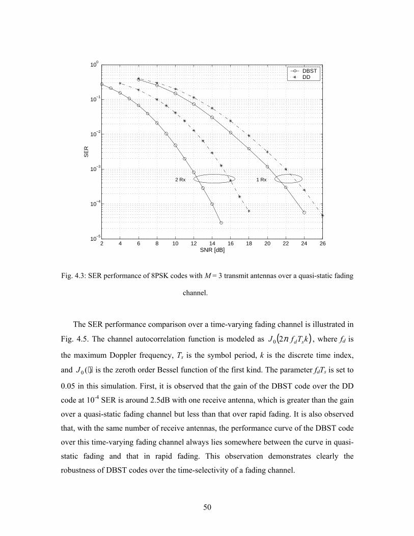
2 4 6 8 10 12 14 16 18 20 22 24 2610

−5

10−4

10−3

10−2

10−1

100

SNR [dB]

SE

R

1 Rx2 Rx

DBSTDD

Fig. 4.3: SER performance of 8PSK codes with M = 3 transmit antennas over a quasi-static fading

channel.

The SER performance comparison over a time-varying fading channel is illustrated in

Fig. 4.5. The channel autocorrelation function is modeled as ( kTfJ sd )π20 , where fd is

the maximum Doppler frequency, Ts is the symbol period, k is the discrete time index,

and is the zeroth order Bessel function of the first kind. The parameter f)(0 ⋅J dTs is set to

0.05 in this simulation. First, it is observed that the gain of the DBST code over the DD

code at 10-4 SER is around 2.5dB with one receive antenna, which is greater than the gain

over a quasi-static fading channel but less than that over rapid fading. It is also observed

that, with the same number of receive antennas, the performance curve of the DBST code

over this time-varying fading channel always lies somewhere between the curve in quasi-

static fading and that in rapid fading. This observation demonstrates clearly the

robustness of DBST codes over the time-selectivity of a fading channel.

50

2 4 6 8 10 12 14 16 18 20 22 24 2610

−5

10−4

10−3

10−2

10−1

100

SNR [dB]

SE

R

1 Rx2 Rx

DBSTDD

Fig. 4.4: SER performance of 8PSK codes with M = 3 transmit antennas over a rapid fading

channel.

To sketch the performance enhancement of other DBST codes in Table 4.1 to 4.3

over DD codes, we select the ones with M = 2 transmit antennas and evaluate their

required operating SNR’s, respectively, at a specified SER of 2 over a rapid fading

channel. The results are reported in Table 4.4, from which it is seen that the asymptotic

improvement predicts the actual SNR reduction very well, especially at more than

one receive antenna. A histogram of the results is also plotted in Fig. 4.6.

410−×

∞∆

51

2 4 6 8 10 12 14 16 18 20 22 24 2610

−5

10−4

10−3

10−2

10−1

100

SNR [dB]

SE

R

1 Rx2 Rx

DBSTDD

Fig. 4.5: SER performance of 8PSK codes with M = 3 transmit antennas over a time-varying

fading channel with . 05.0=sdTf

Table 4.4: Operating SNR [dB] at SER = 2 for codes with M = 2 transmit antennas over a

rapid fading channel

410−×

1 Rx 2 Rx SNRDBST SNRDD gain SNRDBST SNRDD gain QPSK 22 22.24 0.24 12.86 13.13 0.27 8PSK 25.33 27.74 2.41 15.48 18.5 3.02

16PSK∗ 29.34 33.6 4.26 18.9 24.47 5.57 32PSK* 33.15 39.56 6.41 21.84 30.42 8.58 64PSK 35.9 45.5 9.6 14.42 24.76 10.34

∗ Suboptimal codes from Table III

52

QPSK 8PSK 16PSK 32PSK 64PSK0

1

2

3

4

5

6

7

8

9

10

11

Modulation Level

Gai

n [d

B]

1Rx 2Rx

Fig. 4.6: Histogram of the gains shown in Table 4.4.

4.4.2 Comparison with Other Existing Codes

Through exhaustive search, authors in [33] provided several QPSK and 8PSK codes with

three and four transmit antennas for quasi-static flat fading channels based on the

Euclidean distance criterion. In particular, they designed 8PSK codes with up to 32 trellis

states with the order of transmit antenna diversity equal to 2. Comparisons in this

subsection are done between the 32-state 8PSK codes in [33] and our 8PSK codes at the

same number of transmit antennas. The transmission rate is the same for all the codes,

that is, 3 bit/s/Hz. But the number of trellis states is different. Our 8PSK codes with M =

3 and 4 have 64 and 512 trellis states, respectively. To have rather fair comparisons, a

suboptimal tree decoding algorithm is applied in the simulation of our 512-state code: the

M-algorithm [65]. In this algorithm, only a certain number of most likely states, denoted

53

as K, are kept and the remaining states are deleted at each decoding stage. Thus the

decoding complexity is O(K). In our case, K = 64. Fig. 4.7 illustrates the FER

performance comparison over a quasi-static fading channel with frame length T = 130. As

can be seen in this figure, a higher diversity order is achieved by our DBST codes. As a

result, even though our codes perform worse with two receive antennas, superior

performance is achieved with one receive antenna. This is because full transmit diversity

is necessary at high SNR with limited number of receive antennas, while the minimum

Euclidean distance is the dominating factor at low SNR with high enough total diversity

order, as claimed in Chapter 3. The codes in [33] have much larger minimum Euclidean

distance but smaller transmit diversity order than our codes. Hence, the observation in

Fig. 4.7 is not surprising.

6 8 10 12 14 16 18 20 22 2410

−3

10−2

10−1

100

SNR [dB]

FE

R

1 Rx2 Rx

M=3, 64−state DBSTM=4, 512−state (K = 64) DBSTM=3, 32−state in [33]M=4 32−state in [33]

Fig. 4.7: FER performance of 8PSK codes with M = 3, 4 transmit antennas over a quasi-static fading channel.

54

4.5 Summary

In this chapter we proposed an efficient and systematic space-time coding scheme:

diagonal block space-time coding. It is basically a two-step approach: first, construct a 1-

D nonbinary block code; then, apply the diagonal transmission pattern to send the block

code outputs through multiple transmit antennas. It was shown that the diagonal

transmission pattern promises a transmit (spatial and temporal) diversity of order M in a

system with M transmit antennas under both quasi-static and rapid flat fading channels,

while a carefully designed nonbinary block code assures good coding advantage. The

conventional delay diversity code is a special case of this coding scheme when the block

code is a repetition code. To design the optimal block code that maximizes the coding

advantage, two general problems were formulated, namely, the permutation optimization

for a given constellation and the constellation optimization. In particular, we proposed an

efficient linear block code construction over rings for multi-level PSK modulation.

Through simple computer search, we obtained some optimal and suboptimal code

examples using PSK and QAM modulations with 2~6 bit/s/Hz transmission rate and 2~6

transmit antennas. Simulation results showed that they possess significant advantage over

the original delay diversity codes in not only quasi-static fading and rapid fading channels

but also general time-varying fading channels. They also demonstrate superior

performance over the existing codes optimally designed based on the Euclidean distance

criterion with one receive antenna.

The proposed coding scheme is suitable for an arbitrary number of transmit antennas

with arbitrary signal constellations. It can also be easily extended to frequency-selective

fading channels. As it is designed for achieving full transmit antenna diversity with good

coding advantage, this coding scheme has particular application for the downlink

transmission where the base station is capable of installing multiple antennas while the

hand-held mobile station has only one antenna.

55

Chapter 5

GENERALIZED LAYERED SPACE-TIME

ARCHITECTURE

In Chapter 3 and 4, we proposed improvements on the design of space-time codes aiming

at minimizing the error probability at different scenarios. The transmission efficiency of

this type of transmission scheme is, however, constrained by the signal modulation level.

In this chapter, we provide a comprehensive study on generalized layered space-time

architecture (GLST), which can provide a flexible tradeoff between error probability and

transmission efficiency with reasonable complexity.

The basic framework of this architecture is to partition all the available transmit

antennas into several groups and apply space-time coding (STC) as component codes for

each group. At the receiver, to avoid the huge complexity of joint decoding of all groups,

each component space-time code is decoded individually through a serial processing

similar to VBLAST detection algorithm [4, 5] and combines group interference

suppression and group interference cancellation. Hence GLST can be viewed as a

combination of VBLAST and STC. On one hand, the signals transmitted within each

antenna group are space-time coded. Hence higher transmit antenna diversity can be

achieved compared with pure VBLAST. On the other hand, the overall spectral efficiency

is higher than pure STC due to the independence of the signals transmitted by different

antenna groups. Similar ideas can be found in [19] and [40], where space-time trellis

codes and space-time block codes are combined with VBLAST, respectively. We

generalize both of them in this chapter. In addition, we study several features embedded

in the generalized layered architecture to enhance the overall system performance,

including various signal-to-antenna mappings, power allocation and decoding order. To

further improve the system performance of GLST, we propose a computationally

efficient hard-decision iterative decoding scheme. This decoding algorithm performs

almost as good as the optimal ML decoding with much lower complexity.

56

This chapter is organized as follows. In Section 5.1 we introduce the symbol model of

GLST, including the basic encoding and decoding process. The optimal power allocation

and optimal decoding order are derived in Section 5.2 and 5.3, respectively. The iterative

decoding is proposed in Section 5.4. Finally Section 5.5 provides a summary.

The results in this chapter are published in [Tao4, Tao8, Tao9].

5.1 System Model


antennas as shown in Fig. 2.3. It is assumed that the channel is quasi-static flat Rayleigh

fading and the channel coefficients are perfectly known to the receiver. The basic

encoding and decoding process are described as follows.

S/P

STC1

B

B1

STC2

B2

STCq

Bq

C1 INT1

C2 INT2

Cq INTq

INT

(a)

α1 Tx 1,2

β1

γ1 Tx 5,6

Tx 3,4

α2 α3

β2 β3

γ2 γ3

t

α4

β4

γ4

α1 Tx 1,2

β1

γ1 Tx 5,6

Tx 3,4

γ2β3

α2γ3

β2α3

t

α4

β4

γ4

(b) (c)

Fig. 5.1: Encoder of (interleaved) GLST (a) main layout, (b) HGLST, and (c) DGLST.

57

5.1.1 Encoding

The encoding process of GLST is illustrated in Fig. 5.1. A block of B input information

bits is transformed by a serial-to-parallel (S/P) converter into q groups of bit stream of

length B1, B2, …, Bq, with . Each group of bit stream, BBBBB q =+++ K21 j, for 1 ≤ j ≤

q, is then separately encoded by a component space-time encoder STCj associated with

Mj Tx antennas, with M1 + M2 + … + Mq = M. The output Mj × T codeword matrix Cj is

to be transmitted by Mj antennas over T time intervals. The t-th column of Cj, denoted by

cj,t, is referred to as the symbol vector of group j at time t. Before transmission, the

symbol vectors from each group are passed through an individual temporal interleaver

followed by a spatial interleaver. The temporal interleavers are labeled by the dashed

block in Fig. 5.1(a) and will be discussed in Section 5.4. The spatial interleaver is

interpreted as a mapping from the symbol vectors to the transmit antennas at each symbol

period. We consider two special mappings, namely, horizontal mapping and diagonal

mapping, shown in Fig. 5.1(b) and (c), respectively.

The horizontal mapping is to simply pass all the symbol vectors from one group to a

fixed group of antennas. A simple example is shown in Fig. 5.1(b), where αt, βt, and γt,

with t = 1, 2, …, denote the symbol vectors from three different groups and each group is

associated with two transmit antennas. Thus, the transmitted symbol vectors from every

group form a row, or equivalently horizontal pattern and we refer to such GLST as

HGLST. In the diagonal mapping, the symbol vectors from each group cyclically utilize

different group of antennas at different symbol intervals with period p. A simple example

is illustrated in Fig. 5.2(c) with p = q = 3. Hence the transmitted symbol vectors from

every group are allocated in a diagonal pattern across the antenna and time dimensions.

We call such GLST as DGLST. Since the channel seen by the symbol vectors from each

group changes periodically, additional antenna diversity can be achieved in DGLST

compared with HGLST. It is noticed that the diagonal mapping considered in this paper

is different from the diagonal transmission pattern in [3], where zero-padding was

required at the beginning and the end of each transmission frame and hence the spectral

efficiency was reduced.

58

5.1.2 Decoding

Let rt denote the N × 1 received signal vector at time instance t in GLST. It can be written

as

ttqtqttttr wcHcHcHr ++++= ,,,2,2,1,1 L (5.1)

where Hj,t denotes the N × Mj subchannel matrix of group j at time t and wt denotes the

additive complex Gaussian noise term.

The layered structure of GLST allows a similar serial decoding as in VBLAST

systems, except that all the interference nulling and interference cancellation are group

based. The serial decoding order will be discussed in Section 5.3. In this subsection, we

assume it is already determined and denoted by, without loss of generality, {1’, 2’, …,

q’}. The decoding algorithm is the following.

At the first decoding level (j = 1), we let = r1tr t, for all 1 ≤ t ≤ T.

At the j-th decoding level, given that the previous j-1 groups 1’, 2’, …, (j-1)’ have

already been decoded and cancelled out from the received signals, the resulting received

signal for t =1, …, T, which still contains interference from the not-yet-decoded

groups (j+1)’, (j+2)’, …, q’, can now be written as,

jtr

jttqtqtjtjtjtj

jt vcHcHcHr ++++= ++ ,',',)'1(,)'1(,',' K . (5.2)

Then at each time t, we can find a set of orthonormal row vectors (not necessary unique)

in the null space of [H(j+1)’,t, …, Hq’,t], and form them into an (

nulling matrix . Multiplying with r suppresses all the signals from groups

(j+1)’ to q’ and generates the interference free decision signal for group j’

mnnnm j ×+++− )''1 L

jtW j

tW jt

jttjtj

jt

jttjtj

jt

jt

jt

jt vcHvW0cHWrWr ~~~

,',','', +=++== . (5.3)

It is seen that tj ,'~H

jtv

is the equivalent channel matrix at time t for group j’, whose entries

are independent and identically complex Gaussian distributed with mean zero and

variance 0.5 per dimension. Assuming perfect interference cancellation, the equivalent

noise vector ~ also contains independent and identically complex Gaussian distributed

entries [19].

59

As for the nulling matrix , we have = WjtW j

tW j for all 1 ≤ t ≤ T in HGLST since the

channel seen by each group is time-invariant in each transmission frame. This implies

that the nulling matrix is only calculated once for each frame. While in DGLST, since the

channel seen by each group varies with period p, we have = . Hence the total

number of p nulling matrices are required for each frame.

jtW j

pt modW

Now the j’-th codeword can be decoded using ML space-time decoder based on jtr

~

in (5.3)

∑=

−=T

tttj

jtj

1

2,''

~~minargˆ cHrCC

. (5.4)

Before moving on to the next decoding level, we subtract the contribution of the just

decoded group j’ from and it results in the modified received signal jtr 1+j

tr

Tttjtjj

tj

t ≤≤−=+ 1,ˆ ,','1 cHrr . (5.5)

We restart the above procedure for j = j + 1, until all groups are decoded (j = q).

Different from BLAST, the requirement for the number of receive antennas in GLST

is N ≥ M - M1’ + 1. Particularly, if the decoding order depends on the channel realization

for each transmission frame at the receiver, 1’ could be any integer from 1 to q. Hence to

guarantee that the system works, we let N ≥ . 1}{max +− jjMM

5.2 Optimal Power Allocation

It is seen from the above decoding procedure that, if the decoding order is pre-determined

and independent of the channel realizations at the receiver, group j’ decoded at the j-th

decoding level has the antenna diversity of order Mj’ (N−M + M1’ + … + Mj’). Assume M1

= M2 = … = Mq, and all groups employ the same STC and are assigned the same

transmission power, then group 1’ would have the worst performance. As the overall

system performance is usually limited by the group with the worst performance,

improving the performance of group 1’ will be most effective in enhancing the overall

system performance. Unless specified otherwise, the STCs employed for all groups are

identical in this paper. Then the most straightforward method to enhance the system

60

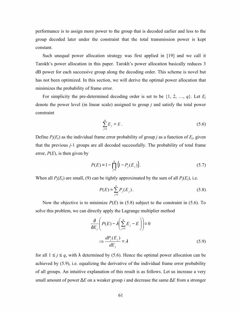
performance is to assign more power to the group that is decoded earlier and less to the

group decoded later under the constraint that the total transmission power is kept

constant.

Such unequal power allocation strategy was first applied in [19] and we call it

Tarokh’s power allocation in this paper. Tarokh’s power allocation basically reduces 3

dB power for each successive group along the decoding order. This scheme is novel but

has not been optimized. In this section, we will derive the optimal power allocation that

minimizes the probability of frame error.

For simplicity the pre-determined decoding order is set to be {1, 2, …, q}. Let Ej

denote the power level (in linear scale) assigned to group j and satisfy the total power

constraint

EEq

jj =∑

=1. (5.6)

Define Pj(Ej) as the individual frame error probability of group j as a function of Ej, given

that the previous j-1 groups are all decoded successfully. The probability of total frame

error, P(E), is then given by

( )∏=

−−=q

jjj EPEP

1)(11)( . (5.7)

When all Pj(Ej) are small, (9) can be tightly approximated by the sum of all Pj(Ej), i.e.

∑=

≈q

jjj EPEP

1)()( . (5.8)

Now the objective is to minimize P(E) in (5.8) subject to the constraint in (5.6). To

solve this problem, we can directly apply the Lagrange multiplier method

0)(1

=

−−

∂∂ ∑

=EEEP

E

q

jj

j

λ

λ=⇒j

jj

dEEdP )(

(5.9)

for all 1 ≤ j ≤ q, with λ determined by (5.6). Hence the optimal power allocation can be

achieved by (5.9), i.e. equalizing the derivative of the individual frame error probability

of all groups. An intuitive explanation of this result is as follows. Let us increase a very

small amount of power ∆E on a weaker group i and decrease the same ∆E from a stronger

61

group j. If the reduced individual frame error probability ∆Pi of group i is larger than the

increased individual frame error probability ∆Pj of group j, then we can say that the total

frame error probability is decreased. We can keep increasing the power on group i and

decreasing the power from group j as long as the corresponding ∆Pi is larger than ∆Pj.

The power exchange between the two groups can be stopped once ∆Pi and ∆Pj are equal,

i.e. the total frame error probability cannot be decreased anymore. Overall, the power

should be allocated in such a way that any small enough amount of power change will

have the same effect on all individual frame error probabilities. Mathematically, the

derivative of the individual frame error probabilities is the same, as shown in (5.9).

As the power allocation scheme does not depend on the channel information, the

optimization can be done offline for a target operating SNR. Hence the system

complexity is unchanged.

Theoretically obtaining the precise function for Pj(Ej) in GLST system is

complicated. In this paper we produce an approximate function using computer

simulation and curve fitting technique. We perform real interference nulling and space-

time decoder steps but ideal interference cancellation step, meaning the contribution from

the just decoded group is perfectly known and cancelled out at each decoding level. The

individual frame error probability for each group is then simulated and plotted as a

function of the power. Afterwards, curve fitting is applied on each curve and thus an

approximate function of the individual frame error probability is obtained for each group.

Simulation has been performed to evaluate the superiority of the proposed optimal

power allocation. For brevity, we use the notation (M, N) from now on to denote a MIMO

system with M transmit antennas and N receive antennas. The simulation setup is as

follows and it will be used in all the simulations in this paper. We take two GLST

systems as examples: (4, 4) GLST and (8, 8) GLST. Each system includes both HGLST

and DGLST versions. For simplicity, each group contains two antennas. The 2 bit/s/Hz

QPSK modulated 16-state space-time trellis code given in [8, Fig. 5] is taken as the

component code for all the groups. Thus the transmission rate of the two systems is 4

bit/s/Hz and 8 bit/s/Hz, respectively. We consider quasi-static flat Rayleigh fading

channels. The channel coefficients are assumed perfectly known at the receiver. Each

62

frame contains 130 transmission from each transmit antenna, which corresponds to 520

and 1040 information bits per frame at the (4, 4) and (8, 8) systems, respectively.

Fig. 5.2 shows the frame error rate (FER) performance versus the average received

SNR per receive antenna in the (4,4) and (8,8) systems. The curve fitting function for the

optimal power allocation we used in this simulation is ( ))(exp)( jjj EfEP = , where

is a third order polynomial function of E)( jEf j. We can see that, the improvement of the

optimal power allocation over equal power allocation (i.e. no power allocation) is about

1.5 dB and 3.5 dB at a FER of 0.01 in the (4,4) and (8,8) systems respectively. It is also

seen that, in the (4,4) system, the gain of the optimal power allocation over Tarokh’s

power allocation increases as the SNR increases, while in the (8,8) system, the gain at

low SNR is larger than the gain at high SNR.

Another observation from Fig. 5.2 is that DGLST generally performs better than

HGLST. This is as expected due to the additional diversity introduced by diagonal

mapping.

7 8 9 10 11 12 13 14 15

10−3

10−2

10−1

100

SNR [dB] per receive

Fra

me

Err

or R

ate

HGLST equal PA HGLST Tarokh PA HGLST optimal PADGLST equal PA DGLST Tarokh PA DGLST optimal PA

(a)

63

8 9 10 11 12 13 14 15 16 1710

−3

10−2

10−1

100


Fra

me

Err

or R

ate

HGLST equal PA HGLST Tarokh PA HGLST optimal PADGLST equal PA DGLST Tarokh PA DGLST optimal PA

(b)

Fig. 5.2: Performance comparison of different power allocation in the (a) (4,4) and (b) (8,8) GLST systems.

5.3 Optimal Decoding Order

In the previous section we discussed the power allocation to enhance the system

performance when the decoding order is independent of CSI. In this section we will

demonstrate how to determine the decoding order based on the channel realizations at the

receiver when no power allocation is applied. Notice that, the decoding order in DGLST

systems is not important and can be arbitrary as different groups see the same time-

varying channels. Hence we only consider HGLST in this section.

At the first decoding level (j = 1), let H1 = [H1, …, Hq], where Hl is the N × Ml

subchannel matrix corresponding to group l, and define the candidate group set as S1≡{l

|1 ≤ l ≤ q}.

At the j-th decoding level, for each l∈ Sj, we find a set of orthonormal row vectors

in the null space of jl

H , where jl

H denotes the matrix obtained by eliminating Hl from

64

Hj, and use them to form an ( matrix . Then we

left-multiple H

NMMMMN ll ×++++− − ))'1('1 L

lj

ljl HWH =

jlW

l by to obtain the equivalent channel matrix of group l at this

decoding level

jlW

~

2⋅

2~maxarg' jlSl j

j H∈

=

}'{\1 jSS jj =+

jj

j'

1 HH =+

( 1 jMMM −−− K

)'1 −

.

As the post-detection SNR defined on the whole codeword from each group is

proportional to the squared Euclidean norm [74] of the corresponding equivalent

channel matrix, we choose the candidate with the largest squared Forbenius norm as the

group to be decoded at this level

. (5.10)

Then we update the candidate group set as, by removing j’ from Sj,

.

The channel matrix is correspondingly changed to, by eliminating Hj’ from Hj,

.

This process continues for j = j+1 until the candidate set becomes empty. The decoding

order is now obtained as {1’, 2’, …, q’}, which is a certain permutation of {1, 2, …, q}.

As BLAST order was shown to be optimal in the sense of minimizing the probability

of frame error [6], the above decoding order (5.10) can also be similarly shown to be

optimal in the same sense and we omit the proof.

To this stage, let us compare the complexity among HGLST with arbitrary (or pre-

determined) decoding order, HGLST with optimal decoding order and DGLST with

arbitrary decoding order (no optimal decoding order for DGLST). First we consider the

complexity of performing interference nulling measured by the computation of finding

the null space basis of a two-dimensional complex matrix. At the j-th decoding level of

HGLST with arbitrary decoding order, say {1, 2, …, q}, it requires computation of

finding the null space basis of an N × ) matrix. At the j-th decoding

level of HGLST with optimal decoding order {1’, 2’, …, q’}, to determine which group

will be decoded, the computation of finding the null space basis of an N ×

matrix has to be done for every l∈ S)( ('1 lj MMMM −−− −K j. While at the j-th

65

decoding level of DGLST with arbitrary decoding order, say {1, 2, …, q} also, it requires

computation of finding null space basis of p different N × matrices.

Let M

)

( 1 jMMM −−− K

1 = M 2 = … = M q and treat the complexity of performing interference nulling in

HGLST with arbitrary decoding order as benchmark. Then at the j-th decoding level with

1 ≤ j ≤ q − 12, the complexity in DGLST with arbitrary decoding order and HGLST with

optimal decoding order is q and q − j − 1 times higher, respectively. As the complexity of

computing the squared Euclidean norm in HGLST with optimal decoding order can be

ignored compared to that of finding null space basis, we see that before doing the ML

decoder process for each component STC, DGLST has the highest complexity and

HGLST with arbitrary decoding order has the lowest complexity. Once the decoding

order and the nulling matrices are computed, the complexity of the following decoding

process is the same for all of them.

Fig. 5.3 provides the FER performance of the optimal ordered decoding in the (4,4)

and (8,8) HGLST systems. We first observe that with optimal ordered decoding the FER

performance of HGLST is enhanced by around 2dB and 3.5dB in the (4,4) and (8,8)

systems, respectively. Comparing Fig. 5.3 with Fig. 5.2, we then observe that HGLST

with optimal ordered decoding performs slightly better than HGLST with optimal power

allocation, but slightly worse than DGLST with optimal power allocation.

For reference, we also provide the performance of the (4,4) and (8,8) BLAST and

coded BLAST systems in Fig. 5.3. In BLAST systems, the data symbols are BPSK

modulated. In coded BLAST systems, each layer is encoded individually by the rate ½

convolutional code with constraint length K = 5. The coded bits are Gray-mapped to

QPSK modulation. And the soft-decision Viterbi decoder, instead of the symbol-by-

symbol detector, is used for interference cancellation. From the slopes of the performance

curves, it is seen that the diversity order of HGLST is higher than BLAST and it results in

significant performance improvement even under roughly the same complexity.

2 Interference nulling is not required at the last decoding level.

66

7 9 11 13 15 17 1910

−3

10−2

10−1

100


Fra

me

Err

or R

ate

BLAST optimal order coded BLAST optimal oderHGLST arbitrary order HGLST optimal order

(a)

8 10 12 14 16 18 20

10−3

10−2

10−1

100


Fra

me

Err

or R

ate

BLAST optimal order coded BLAST optimal oderHGLST arbitrary order HGLST optimal order

(b)

Fig. 5.3: Performance comparison of optimal ordered decoding in the (a) (4,4) and (b) (8,8)

GLST and BLAST systems.

67

5.4 Interleaved GLST with Hard Decision Iterative Decoding

The above serial decoding scheme has not taken full advantage of the receive antenna

diversity yet. Particularly, the receive antenna diversity order of group j’ decoded at the j-

th decoding level is only N – M + M1’ + … + Mj’. Therefore, we propose an iterative

decoding process that can efficiently enable all groups to achieve full receive antenna

diversity. To eliminate the effect of burst error propagation among groups during

iterations we insert different temporal interleavers on the codewords from different

groups. This is shown in Fig. 5.1(a) and called interleaved GLST. Each interleaver is

vector based with vector size equal to the spatial dimension of the relevant codeword.

This ensures that the rank property of STC in each group is not destroyed.

The iteration procedure is depicted in Fig. 5.4. The first iteration is the same as

described in Section 5.1.2 except that interleaving and deinterleaving must be done

accordingly. The serial decoding order shown in this figure is {1’, 2’, …, q’}, without

loss of generality, for both optimal and arbitrary (or pre-determined) decoding order. At

the subsequent iterations, since all groups have been decoded already, interference

nulling is no longer needed. Instead, interference cancellation is performed for all groups.

Each iteration is composed of q levels, and each level is processed successively at the

same order as in the first iteration. At level j, we subtract the interference made by group

1’, …, (j-1)’, (j+1)’, …, q’ from the original received signals and re-decode group j’

using ML decoder. Once decoded, the new decision of group j’ is fed back to the next

level for decoding group (j+1)’. One iteration is finished when all the q levels are

finished. We can stop the iteration when the decoded signals are reliable.

An important note for the proposed iterative decoding algorithm is that, all the

interference cancellation is hard decision, and the ML space-time decoder becomes

Viterbi decoder or simple linear processing for space-time trellis codes and space-time

block codes, respectively. This guarantees low complexity compared with the

conventional turbo processing [38, 39, 40], where soft interference cancellation and

maximum a posteriori probability (MAP) decoder were used.

68

IC

P/SOutput

IN

adder

ST Dec-Enc 1’

IC

ST Dec-Enc 2’

IC

ST Dec-Enc q’

ST Dec-Enc 1’

IC

adderST Dec-Enc 2’

adder

ST Dec-Enc q’

adder

ST Dec-Enc 1’

adder

ST Dec-Enc 2’

adder

ST Dec-Enc q’

IC

IC

IC

IC

IC

B

C

B

C

B

C

C

1st iteration 2nd iteration kth iteration

IN

(a)

deint j’ STC j’ Decoder STC j’ Re-coder int j’ r C

B

(b)

Fig. 5.4: Iterative decoding of interleaved GLST (a) main block diagram, (b) sub-block diagram

for the “ST Dec-Enc j’” component.

To evaluate the results of the interleaved GLST with iterative decoding we first take

the HGLST version with optimal decoding order as an example to do simulation. All the

interleavers in our simulation are pseudo-random with depth equal to the frame length.

The results are shown in Fig. 5.5. We consider the (4, 4) HGLST system shown in Fig.

5.5(a) first. It is observed that the iterative decoding with interleaver dramatically

improves the performance. With three iterations it achieves 2.5 dB gains at 0.01 FER

when compared with the required SNR using the optimal ordered decoding found in Fig.

5.3(a). To study the role of interleaver we also provide the simulation results of the

iterative decoding without interleaver. We see that the interleaver has no gain at the first

iteration but brings significant gain at the subsequent iterations. As discussed above, the

first iteration procedure is the same as the basic serial decoding. Hence the performance

is limited by the group decoded first with the lowest diversity gain. As interleaver is

useless for the first group, it thus has little effect on the first iteration. However, from the

69

second iteration on, interleaver helps significantly in spreading out burst errors among

groups. It is seen that, with three iterations, the loss due to imperfect interference

cancellation (IC) with interleaver is only 0.6 dB, while the loss due to severe error

propagation without interleaver is 1.6 dB at 0.01 FER. Little gain can be achieved by

more than three iterations. Similar performance comparison for the (8, 8) HGLST system

is shown in Fig. 5.5(b). The improvement achieved by the iterative decoding with

interleaver is even larger. With four iterations, it provides a gain of 5.6 dB over the

optimal ordered decoding at 0.01 FER when compared with Fig. 5.4(b). The loss due to

imperfect IC with interleaver is now only 0.25 dB, while the loss due to severe error

propagation without interleaver is more than 2 dB at 0.01 FER. The gain achieved after

four iterations is very small.

We also provide the performance of interleaved DGLST with iterative decoding in

Fig. 5.6. We can see that with the same iterations HGLST is slightly inferior to DGLST

at low SNR but performs better at high SNR.

5.5 Summary

In this chapter, generalized layered space-time coding, a combination of BLAST and

STC for MIMO systems was introduced. In particular HGLST and DGLST were

classified according to different mappings from signals to transmit antennas. The basic

decoding of GLST is a certain ordered serial processing that combines group interference

nulling and group interference cancellation techniques. For the decoding with order pre-

determined and independent of the channel, optimal power allocation was derived to

enhance the system performance without increasing the complexity. This approach is

suitable for all GLST systems. For HGLST systems without power allocation, we also

discussed the optimal decoding order. To fully utilize the advantage of receive antenna

diversity, interleaved GLST with iterative decoding was further proposed. This iterative

decoding applies hard interference cancellation and ML decoder for component codes,

thus has much lower complexity than conventional turbo processing which requires soft

interference cancellation and MAP decoder.

70

4 5 6 7 8 9 1010

−3

10−2

10−1

100


Fra

me

Err

or R

ate

1st ite w/ int2nd ite w/ int3rd ite w/ int1st ite w/o int2nd ite w/o int3rd ite w/o intPerfect IC bound

(a)

4 4.5 5 5.5 6 6.5 7 7.5 8 8.5 9

10−3

10−2

10−1

100


Fra

me

Err

or R

ate

1st ite w/ int2nd ite w/ int4th ite w/ int1st ite w/o int2nd ite w/o int4th ite w/o intPerfect IC bound

(b)

Fig. 5.5: Performance of iterative decoding in the (a) (4,4) and (b) (8,8) HGLST systems.

71

2 3 4 5 6 7 8 9 10 1110

−3

10−2

10−1

100


Fra

me

Err

or R

ate

(4,4) HGLST,3rd(4,4) DGLST,3rd(8,8) HGLST,4th(8,8) DGLST,4th

Fig. 5.6: Performance comparison of interleaved HGLST and interleaved DGLST with iterative

decoding in the (4,4) and (8,8) systems.

Based on the simulation results we conclude that GLST provides a promising solution

achieving high data rate and high quality communications in multiple-antenna systems,

especially when the number of antennas is large.

72

Chapter 6

DIFFERENTIAL SPACE-TIME BLOCK CODES

The schemes we proposed in Chapter 3 to Chapter 5 are all based on the assumption that

the channel knowledge is available at the receiver. This is reasonable when the channel

varies slowly enough that pilot signals can be used for channel estimation. In mobile

environments, however, precisely tracking the channel variation becomes difficult,

especially in a system with a large number of antenna elements. Hence, in this chapter

and the following one, we propose enhancements on the non-coherent space-time

techniques that can avoid channel estimation at the receiver, but with minimal loss in

error performance.

In this chapter we propose a differential space-time modulation scheme based on the

orthogonal space-time block codes (STBC) having square codeword matrices in [9] when

neither the transmitter nor the receiver has access to channel state information. The

decoupling property retained by coherent STBC can still be exploited, which results in

simple linear decoding complexity. This work is different from the previous work by

Tarokh and Jafarkhani in [58] in two aspects. First, the restriction of constant-amplitude

modulation (PSK) on information data symbols is relaxed such that more efficient multi-

amplitude constellations, such as QAM, can be applied. Simulation results show that a

gain of 3 ~ 4 dB can be achieved by using 16QAM rather than 16PSK modulation with

almost no increase on the detection complexity. Second, this differential scheme is not

only suitable for Alamouti’s block code with two transmit antennas, but also for any

orthogonal block codes with an arbitrary number of transmit antennas as long as the

codeword matrices are square.

Moreover, we compare the proposed differential orthogonal space-time block codes

(DSTBC) with existing diagonal cyclic group codes [57, 55]. The advantages are not only

in lower decoding complexity, but also in better performance. It is shown that a

significant improvement up to 6~8 dB can be achieved in a system with two transmit

antennas and one receive antenna over a slowly time-varying flat fading channel.

73

This chapter is organized as follows. In Section 6.1 we briefly introduce the system

model. In Section 6.2 we describe the proposed DSTBC in detail. The differentially non-

coherent decoding methods are derived in Section 6.3. Section 6.4 provides some

simulation results and Section 6.5 summarizes this chapter.

The following terminology is used throughout this chapter. For an M × M orthogonal

matrix A with AAH = AHA = a2I, we say the nonnegative scalar, a, is the amplitude of A.

The results in this chapter are published in [Tao7].

6.1 System Model


antennas as shown in Fig. 2.3. The channel is assumed to be flat Rayleigh fading and

remains constant within T symbol periods. The M × T transmitted signal matrix is

denoted by C and satisfies the total energy constraint

E[tr(CCH)] = T. (6.1)

Let R denote the N × T received signal matrix. It can be written as

WHCR += sρ (6.2)

where H is the N × T channel matrix with i.i.d. and zero-mean unit-variance complex

Gaussian distributed entries, W contains i.i.d complex Gaussian noise terms with zero

mean and variance σ2, and ρs is the average transmitted signal energy per symbol period.

The total transmitted SNR can be computed as 2σρρ s= .

Without knowing H and conditioned on C, R contains i.i.d. rows and each row is

complex Gaussian distributed with mean vector 0 and covariance matrix .

Then the probability density function (pdf) of R is given by

CCI Hsρσ +2

( )( )

( )CCI

RCCIRCR H

sNTN

HHs

pρσπ

ρσ

+

+−

=

−

2

12

det

trexp| . (6.3)

One of the interesting observations from (6.3) is that P(R|C) will not change if we left

multiply C by any arbitrary M × M unitary matrix Φ. In other words, C and ΦC are

indistinguishable for non-coherent detection.

74

6.2 Differential Encoding

6.2.1 Data Matrix

In general, an orthogonal space-time block code is described by a set of M × P codeword

matrices, and can be viewed as a mapping from a sequence of modulated data symbols ci,

i = 1, …, K, to a codeword C which is to be transmitted by M antennas over P symbol

periods. Each element of C is a linear combination of c1, …, cK and their conjugates. The

rate for the code is defined as PK . The primary property of a STBC is its orthogonality

M

K

ii

H c ICC ∑=

=1

2 .

In this thesis, we concentrate on square STBCs, i.e., P = M. As we mentioned in Section

2.5.2, for rate-1 code with K = M the real-valued square codes exist for 2, 4, and 8 Tx

antennas, while the complex-valued square codes only exist for 2 Tx antennas (Alamout’s

scheme). For other code rate with K < M, complex-valued square codes can be

constructed.

We assume that each data symbol ci, i=1,…,K is taken from a constellation (e.g. PSK

or QAM, etc) with size q and unit average energy. Then the data matrix in our proposed

DSTBC is defined as V

CVK1= (6.4)

where the factor K1 is used to satisfy the energy constraint in (6.1). Now, or each V

we have

IVV 2aH = (6.5)

with ∑ == K

i icKa1

2/1 being the amplitude of V. If we consider the set of all possible

data matrices to form a constellation V, then V has size of L = qK and satisfies

MH

KH

K qqIVVVV

VV∑∑∈∈

==VV

11 .

75

Particularly, if ci is PSK modulated, a = 1 for all V and such V is called a

constellation with single amplitude. Otherwise, a will take some discrete values and V is

now called a constellation with multiple amplitudes. Note that this is the major difference

between our approach and traditional DUSTM which always has single amplitude. It

potentially allows us to increase the spectral efficiency by carrying information not only

on the orientation but also on the amplitude of a data matrix.

6.2.2 Transmitted Matrix

Similar to DPSK, an identity matrix which does not carry any information is sent by the

transmitter to initialize the transmission, i.e., C0 = IM. Thereafter, the data matrices are

differentially encoded and sent. The transmitted signal matrix at the kth time block is

given by

kkk VCC 1~

−= (6.6)

where Vk is the data matrix at time block k and 1~

−kC is the normalized version of Ck-1

defined as

11

11~

−−

− = kk

k aCC

with ak-1 being the amplitude of Ck-1. Note that the differential encoding function (6.6) is

a little bit different from the traditional equation shown in (2.7), where the amplitude of

Ck-1 is always equal to 1. In addition, the differential transmission scheme proposed in

[58] appears as a special case of our scheme for 2 transmit antennas and PSK modulated

data symbols.

6.3 Non-Coherent Decoding

Two consecutive received signal matrices are used to recover each data matrix at each

time block. We assume that the channel keeps unchanged within T = 2M symbol periods,

then the received matrices can be written as

111 −−− += kksk WHCR ρ (6.7)

76

kksk WHCR += ρ . (6.8)

We derive two non-coherent decoding methods, namely optimal differential decoder (in

the sense of maximum likelihood over two consecutive received signal matrices) and

near-optimal differential decoder.

6.3.1 Optimal Differential Decoder

We stack two consecutive received matrices to form a matrix with T = 2M rows

[ ] [ ] [ ] kkskkkkskkk WCHWWCCHRRR +=+== −−− ρρ 111 .

Then it is easy to show that

( ) MkkHkk aa ICC 22

1 += −

with ak being the amplitude of Ck, or equivalently Vk by (6.6). Substituting the above into

(6.3) yields

( ) ( )

( ) ( )( )

++−+++

=

=

−−−−

∈

∈

221

221122

12 lnmaxarg

|lnmaxargˆ

kksH

kkkkks

s

kkok

aaMNaaa

p

ρσρσ

ρVRR

CRV

V

V

V

V (6.9)

where the matrix formulae

( ) ( )BAIABI +=+ detdet

( ) ( ) 111111 DABDACBAABCDA −−−−−−− +−=+ 1

are employed. Hence the sequence of data symbols ci, i=1,…,K can be jointly decoded by

the inverse mapping from ( )okV̂ .

It is seen from (6.9) that the detection of Vk requires the knowledge of ak-1. This is

contrary to DUSTM where the detection of each data matrix is always independent of the

previously transmitted matrix. At first glance, one may expect that error propagation

would be introduced. However, by simulation in Section 6.3, we show that in the systems

using 16QAM modulated data symbols, there is virtually no error propagation.

77

6.3.2 Near-Optimal Differential Decoder

Substituting (6.6) into (6.8) and then applying (6.7) we can obtain

kkkkkkkk aa WVWVYR +−= −−−−

−− 1

111

11 .

Since the noise matrices at different time blocks are independent and have i.i.d entries,

we can rewrite the above equation as '22

1111 1 kkkkkkk aaa WVRR −

−−−− ++= (6.10)

where is an M × N equivalent noise matrix with entries i.i.d and complex Gaussian

distributed with zero mean and variance σ

'tW

21 ka

2. The insight from (6.10) is that a can

be treated as the known channel matrix for the system transmitting V

111 −

−− kk R

k with noise variance

. Ignoring the dependence of the noise variance on the transmitted signals

acquires the near-optimal differential decoder

21 ka −−+

( ) 21

11minargˆ VRRV

V −−−∈

−= kkknok aV

. (6.11)

Taking advantage of the structure of STBC, it has been shown in [9] that the data

symbols ci, i=1,…,K, can be decoupled and decoded individually from (6.11). As a result,

the near-optimal DD has linear complexity

6.3.3 Optimal DD versus Near-Optimal DD

In this subsection we will consider the constellations with single amplitude and multiple

amplitudes respectively. With single amplitude both ak-1 and ak in (6.9) and (6.11) are

equal to 1. In this case it can be easily verified that the two differential decoders become

equivalent. Moreover, the decoder of Vk is now independent of the previously decoded

matrices. With multiple amplitudes, the near-optimal DD is inferior to the optimal DD

since the variations in the noise variance are ignored. However, the former is much less

complex than the latter. Precisely the complexity of the optimal DD is equal to the size of

the constellation formed by data matrices, i.e. qK, while the complexity of the near-

optimal DD is only a linear function in K, i.e. K × q.

78


In our simulation two channel models are assumed. One is quasi-static flat Rayleigh

fading, i.e. the channel is kept constant within one frame but changed randomly from

frame to frame. Each frame contains 1000 symbol periods besides an initial time block.

The other is time-varying flat Rayleigh fading with autocorrelation ( nTfJ sd )π20

( )⋅0

, where fd

is the maximum Doppler frequency, Ts is the sample period and is the zeroth order

Bessel function of the first kind. The parameter f

J

dTs is set to 0.002.

The two complex-valued square codes G2 with rate 1 and H4 with rate ¾ are taken for

example to demonstrate the performance of our proposed scheme. Their codeword

matrices are given in (2.5) and (2.6), respectively.

Fig. 6.1 and Fig. 6.2 compare the performance of the two non-coherent decoders in

terms of symbol error probability under the quasi-static channel model. The data symbols

are 16QAM, thus the transmission rates are 4 bit/s/Hz and 3 bit/s/Hz for G2 and H4

respectively. It can be seen that the loss due to the near-optimal DD is small compared

with the optimal DD. Hence, the near-optimal DD is selected as the default decoder for

later simulations. Compared with the results of the coherent decoding, the non-coherent

decoding achieves the same order of antenna diversity but with a SNR degradation of 3~4

dB as expected. In these two figures, we also show the performance of the “genied”

optimal DD to indicate the error propagation. “Genied” means that when we use the

proposed optimal DD to recover each data matrix, the amplitude of the past signal matrix

is assumed perfectly known. It is observed that the result of the “genied” optimal DD is

almost the same as the optimal DD, which implies no error propagation.

From Fig. 6.3 to Fig. 6.5 we illustrate the performance comparison in terms of block

error probability between the constellations based on DSTBC with single amplitude

(PSK) and multiple amplitudes (QAM) and the cyclic group constellations suggested for

DUSTM under the time-varying channel model. The block error is defined as the

codeword error. The cyclic group code shown in Fig. 6.3 from M = 2, R = 4 bit/s/Hz is

given in [57, Table I]. It is observed that our proposed DSTBC has significant advantage

over the cyclic group code. The improvement achieved by the constellation with multiple

amplitudes (16QAM) is up to 6~8 dB. Moreover for the same code G2, multiple-

79

amplitude (16QAM) outperforms single-amplitude (16PSK) by 2~3 dB. The cyclic group

code for M = 4, R = 3 bit/s/Hz is not available yet. We only compare the code H4 with

multiple amplitudes (16QAM) and with single amplitude (16PSK) as shown in Fig. 6.4. It

is seen that the former outperforms the latter by 3~4 dB. In Fig. 6.5, the cyclic group code

for M=4, N=1, R=1.98 bit/s/Hz is given in [55, Table I]. The code H4 with 6PSK

modulated data symbols has almost the same transmission rate which is R=1.94 bit/s/Hz

and achieves 1~2 dB improvement.

10 15 20 25 30 35

10−4

10−3

10−2

10−1

100

SNR [dB]

Sym

bol E

rror

Rat

e

Near Optimal DDOptimal DD"Genied" Optimal DDCoherent Decoder

Fig. 6.1: Performance of differential decoding and coherent decoding for G2 with 16QAM data

symbols at M=2, N=1, and R = 4 bit/s/Hz

80

Notice that for the constellations shown in Fig. 6.3 the decoding complexity of the

cyclic group code with differential decoder is equal to the constellation size, i.e.

L=2RM=256, while the complexity of the code G2 with 16QAM modulated data symbols

and with the proposed near-optimal DD is only 2×16=32. For the constellations shown in

Fig. 6.5, the complexities of the cyclic group code with differential decoder and the code

H4 with 6PSK modulated data symbols and with the near-optimal DD (here the near-

optimal DD is equivalent to the optimal DD) are 240 and 18 respectively.

12 14 16 18 20 22 24 26 28 3010

−5

10−4

10−3

10−2

10−1

100

SNR [dB]

Sym

bol E

rror

Rat

e

Near Optimal DDOptimal DD"Genied" Optimal DDCoherent Decoder

Fig. 6.2: Performance of differential decoding and coherent decoding for H4 with 16QAM data

symbols at M = 4, N = 1, and R = 3 bit/s/Hz.

81

10 15 20 25 30 35 4010

−4

10−3

10−2

10−1

100

SNR [dB]

Blo

ck E

rror

Rat

e

Cyclic Group CodeG2 16PSKG2 16QAM

Fig. 6.3: Performance of differential decoder for G2 with 16PSK and 16QAM data symbols and

cyclic group code at M = 2, N = 1 and R = 4 bit/s/Hz.

82

14 16 18 20 22 24 26 28 30 32 3410

−4

10−3

10−2

10−1

100

SNR [dB]

Blo

ck E

rror

Rat

e

H4 16PSKH4 16QAM

Fig. 6.4: Performance of differential decoder for H4 with 16PSK and 16QAM data symbols at M

= 4, N = 1, and R = 3 bit/s/Hz.

83

10 12 14 16 18 20 22 24 26 2810

−4

10−3

10−2

10−1

100

SNR [dB]

Blo

ck E

rror

Rat

e

Cyclic Group CodeH4 6PSK

Fig. 6.5. Performance of differential decoder for H4 with 6PSK data symbols and cyclic group

code at M = 4, N = 1 and R ≈ 2 bit/s/Hz.

6.5 Summary

We presented a differential modulation scheme based on the square STBC over flat

fading channels when neither the transmitter nor the receiver has knowledge of CSI. The

reason why such techniques works and achieves full antenna diversity is that the square

STBCs offer orthogonal property in both spatial and temporal dimensions. Compared

with previous work in [58], our main contributions are as follows. First, the restriction of

PSK modulation for data symbols is relaxed. Second, we extended the DSTBC design

from two transmit antennas to any number of transmitted antennas where square STBC

exists. The advantages of our scheme over cyclic group codes lie in two aspects too,

significant improvement in error performance and considerably low complexity in

84

differential decoding. However, there are also two limitations for our scheme. Since the

constellation formed by data matrices does not form groups, the transmitter needs to

perform matrix multiplication at each time block and the constellation formed by the

transmitted matrices is largely expanded, thus the complexity at the transmitter side is

increased. The second limitation is that, there are only a few square STBCs that have

been designed.

85

Chapter 7

TRELLIS-CODED DIFFERENTIAL UNITARY

SPACE-TIME MODULATION

In Chapter 6, we proposed differential space-time block codes which can be classified

into the general category of differential space-time modulation scheme. However, this

scheme cannot be designed for an arbitrary number of transmitted antennas due to

limitation of STBC itself. Similarly, the design of differential unitary space-time

modulation with good performance and low complexity is still an issue. Notice that all

the differential space-time modulation schemes are actually only non-coherent

modulation schemes over the space-time grid. From the perspective of information

theory, it is necessary to apply channel coding in front of DUSTM to further approach the

channel capacity and hence improve the system performance. In this chapter, we propose

a new trellis coding scheme based on DUSTM, namely trellis-coded DUSTM). This is a

combined trellis coding and space-time modulation scheme, similar to the conventional

trellis-coded modulation (TCM) in single-antenna systems. The advantage of this

combination is that carefully designed trellis codes can effectively help to increase the

minimum distance metric of DUSTM. It results in coding gain and possibly time

diversity gain if an interleaver (matrix-wise) is applied. We thoroughly study the

performance measures and trellis code design rules for systems with either an ideal

interleaver or no interleaver. Several code examples that are based on diagonal cyclic

group constellations [57] and offer a good tradeoff between the coding advantage and

trellis complexity are provided. Extensions to trellis-coded differential space-time block

codes are also discussed. Therein, it is shown that the inherent orthogonality allows to

simply the trellis encoding and decoding and that the conventional well-developed TCM

can be directly applied.

The rest of this chapter is organized as follows. Before we introduce the proposed

TC-DUSTM, some necessary background knowledge on DUSTM is reviewed in Section

86

7.1. In Section 7.2, we present the system model of TC-DUSTM, and derive the

differentially non-coherent decision metrics. Then we propose the trellis code design

criteria. Section 7.3 describes code construction, as well as some code examples. Some

simulation results are shown in Section 7.4. Extensions to the trellis-coded differential

STBC are discussed in Section 7.5. Finally, Section 7.6 summarizes this chapter.

The results in this chapter are published in [Tao1, Tao6].

7.1 Background on DUSTM

The same channel model is considered as in Chapter 6. The encoding process of DUSTM

can be found in Section 2.5.4.

The non-coherent demodulation is based on two consecutive observations Rk-1 and

Rk. We group them into an N × 2M matrix as [ kkk RRR 1−= ] . Similarly we let

[ kkk CCC 1−= ] . It is assumed that the channel is constant within two consecutive time

blocks. Then, by applying (6.3) and using the unitary property of kC , the pdf of kR can

be simplified to

( )[ ]

( )( ) ,|

2

2tr1exp

|

)(

222

)()(

22

klk

MNs

MNMN

HkklH

kls

sk

kk

p

p

VR

RVIV

IIR

CR

=+

+−−

=ρσσπ

ρσρ

σ (7.1)

which is independent of Ck-1. Hence the decision metric of the M × M data matrix Vl(k)

based on the log function of (7.1) can be written, after ignoring irrelevant terms, as

( ) [ ]

{ }2

)(1

or

1)(

or

)()(

)(

trRe

tr,

klkk

kHkkl

HkklH

klkklkm

VRR

RRV

RVIV

IRVR

−

−

−−=

=

=

(7.2)

where Re(⋅) denotes the real part of a complex value. Notice that average transmitted

signal energy ρs and the variance σ2 are not present in the decision metric (7.1). That

implies the receiver does not need to estimate ρs and σ2. Later on, similar observations

87

will be made in the proposed TC-DUSTM. It can also be seen from (7.2) that the

implementation of the decision metric can be either in quadratic form, correlation form,

or minimum distance form. These are all equivalent.

At high SNR, the system performance is determined by the so-called diversity

product ζ of the signal constellation [57]

( ) MllLll

/1''0

detmin21 VV −=

<<≤ζ . (7.3)

Full transmit antenna diversity can be achieved as long as ζ > 0, and a larger ζ results in

better performance. As will be demonstrated in Section 7.2, it is not physically

straightforward to link ζ with the design of TC-DUSTM. Hence, in this thesis, we

reformulate ζ as a new relevant performance parameter, called the determinant distance,

denoted as D. Between any pair of elements Vl and Vl’ in the constellation, we have3

( ) ( ) ( )[ ] ( ) Mll

Mll

HllllD /2

'/1

'''2 detdet, VVVVVVVV −=−−≡ . (7.4)

Indeed, maximizing the minimum D is equivalent to maximizing ζ. Moreover when M =

1,

( )'22''

2 ,),( llllll vvdvvvvD =−= .

Consequently, the determinant distance can be viewed as a novel generalization of

Euclidean distance for signals in matrix form.

7.2 System Model and Performance Measure

7.2.1 System Model

The simplified transmission system diagram under investigation is depicted in Fig. 7.1.

For convenience, we break the trellis-coded unitary space-time modulation (TC-USTM)

into two parts: trellis encoder and USTM mapper. A sequence of information binary bits

b is passed through a rate m / n trellis encoder to generate an encoded bit stream c. Then,

the encoded bit stream c is divided into groups of n bits and each group is mapped at each

3 Based on matrix equations, the squared determinant distance between Vl and Vl’ is also the geometric mean of the eigenvalues of (Vl -Vl’)H(Vl -Vl’).

88

time block k into an element Vl(k) selected from a unitary space-time modulated

constellation with size L = 2n, according to a certain set-partition method. Hence each

transition branch in the trellis corresponds to one coded signal matrix. This is the

combined TC-USTM. Following the encoder, the coded matrix sequence {Vl(k)} is

reordered by a matrix-wise interleaver as {Vl(k’)}. The purpose of the matrix-wise

interleaver is to break the correlation of the fading that affects adjacent coded signal

matrices. The reordered coded matrix sequence from the interleaver is then differentially

encoded as {Ck’} and transmitted by M transmit antennas.

Trellis Encoder

USTM Mapper

Vl(k’) b Matrix-Wise Interleaver

Ck’ = Ck’-1Vl(k’) Ck’

TC-USTM

c Vl(k)

Fig. 7.1: Transmission system diagram of trellis-coded differential unitary space-time modulation

With respect to the interleaver design, we consider two extreme cases. 1) Ideal

interleaver: we assume the system can allow infinite delay such that the length of the

interleaver can be made sufficiently large, then the channel seen by different coded signal

matrices can be assumed to be statistically independent. 2) No interleaver: we assume the

system is delay sensitive and interleavers cannot be used. In the following we are going

to show the decision metrics and design criteria for these two cases respectively.

7.2.2 Ideal Interleaver

At the receiver, the received signal matrix sequence is partitioned

into groups of two blocks in such a way that two adjacent groups are overlapped by one

time block. The overlapping is necessary since the last block in previous group must be

used as a reference in current group for the differential decoding to be applied to each

trellis branch. Note that, due to overlapping, the noise terms in different groups are not

independent. The partitioned sequence is then deinterleaved group by group. The k

[ K10 RRR = ]

th

deinterleaved group and the associated transmitted signal matrices are denoted by the

89

same notations as those in Section 7.1, i.e., kR and kC . Therefore, under the assumption

of ideal interleaver/deinterleaver, both the channel coefficients and the noise terms

contained in different kR are made independent. Hence, given the coded matrix

sequence [ ]K)1( ll VVV = )2( , kR is independent of each other and the joint pdf of R

is simply given by

( ) =p | VR

( ) = pm )|(ln, VRVR

( ))(, klk VR

( )

( ) ( )∏∏ =k

klkk

kk pp )(|| VRCR

where the second equality holds because of (7.1). Hence the decision metric of selecting

the maximum-likelihood (ML) path through the trellis is

( )∑∑ ==k

klkklkk

mp )()( ,)|(ln VRVR (7.5)

where m is the corresponding branch metric. It can be written as any one of

the forms in (7.2). Thus the ML decoding can be efficiently implemented by the soft-

decision Viterbi algorithm.

Let us assume that the transmitted coded matrix sequence is V and the erroneously

decoded sequence is U. Then the pair-wise error probability (PWEP) is given by

( ) ( )

>−=→ ∑∑ VVRURUV 0,, )()(

kklk

kklk mmpP . (7.6)

Applying the Chernoff bound on (7.6) gives

( ) ( ) ( )( )[ ]{ }∏ −⋅−≤→k

klkklk mmEP VURVRUV )()( ,,exp λ (7.7)

where λ ≥ 0 is the Chernoff bound parameter to be optimized. It is observed that the kth

product term in (7.7) is exactly the Chernoff bound of

( ) ( )( ))()()( 0,, klklkklk mmP VVRUR >− ,

which corresponds to the PWEP of an uncoded system ( ))()( klklP UV → . As the explicit

expression of the Chernoff bound of ( ))()( klklP UV → is given by [56]

( ) ( ) ( )

−−+

+−''

2

214det ll

Hll

N VVVVIρ

ρ ,

we obtain the Chernoff bound of the PWEP (7.6) as

90

( ) ( ) ( ) (∏

−−+

+≤→ −

kklkl

Hklkl

NP )()()()(

2

214det UVUVIUV

ρρ ) . (7.8)

Assuming SNR is high enough, the PWEP can be further upper bounded by

( ) ( )∏∈

−−

−

≤→

η

ρk

Nklkl

vMN

P2

)()(det8

UVUV , (7.9)

where η is the set of all k that Vl(k) ≠ Ul(k) and v is the size of η, termed as the Hamming

distance between U and V. From (7.9) it is observed that the achieved diversity order is

the product of antenna diversity MN and the Hamming distance v. Hence, when the

Hamming distance increases by one, the order of diversity increases by MN. This

indicates the substantial advantage of using multiple antennas over single antenna. From

(7.9), it is also observed that the coding advantage is the vth root of the product of the

squared determinant distance

( )v

k

Mklkl

/1/2

)()(det

−∏

∈ ηUV = , ( )

v

kklklD

/1

)()(2

−∏

∈ ηUV

From the two observations, we reach the following design criteria.

Design criteria for the case of ideal interleaver:

• In order to achieve the diversity of order vMN in flat Rayleigh fading channels with

ideal matrix-wise intereleaver, the Hamming distance between any two distinct

coded matrix sequences must be at least v.

• The minimum product of the squared determinant distance between any pair of

coded matrix sequences having the minimum Hamming distance, denoted as

( )min2∏ D , must be maximized.

7.2.3 No Interleaver

In the case without an interleaver, we assume the channel is constant within a certain

period of time, say K + 1 time blocks4. Without the knowledge of CSI at the receiver, the

4 If K is large enough, i.e., slow fading, coherent schemes with chanel estimation may be preferred. Nevertheless, even in slow fading channels, the differential scheme is still reasonable choice in practical systems when the receiver does not want to estimate the channel.

91

pdf of the received matrix sequence R over K + 1 blocks conditioned on the coded matrix

sequence [ ])()2()1( Klll VVV L=V is [53]

( )( )

( )( )MNs

KMNMNK

HH

s

s

K

Kp

ρσσπ

ρσρ

σ

1

1tr1exp

|22)1(

22

++

++−−

=+

RCCIR

VR ,

where ( )[ ])()1()1( Klll VVVIC KL= is the differentially transmitted matrix

sequence. Then we can obtain the ML decision metric as

( ) ( )HHm CRRCVR tr, = . (7.10)

It is seen that (7.10) cannot be simplified to the sum of each branch metric ( ))(, klk VRm

defined in (7.2). A direct implementation of such ML sequence decoding becomes

infeasible. We are seeking a suboptimal decoder that is much less complicated and can be

easily implemented in practice. For each trellis branch, we take into consideration two

consecutive received blocks [ kkk RRR 1−= ] , and compute the total decision metric as

the sum of the branch metrics at all time blocks, i.e.

( ) ( )∑=

=K

kklkmm

1)(,,' VRVR . (7.11)

Therefore, the suboptimal decoder is to select the path through the trellis that has the

largest total decision metric, and can be implemented by the soft-decision Viterbi

algorithm in an efficient manner. Compared with the ML decision metric (7.10), the

suboptimal decision metric (7.11) is a simplified version of (7.10) in which all cross

terms between different Vl(k) are ignored. Nevertheless, the performance gap may be

narrowed by using an approach similar to the multiple-symbol differential detection in

[64] for DPSK in single-antenna systems.

Based on (7.11), we are unable to derive the PWEP due to the memory channel and

non-white Gaussian noise among different kR . However, because we know that DPSK

modulation can be viewed as PSK modulation but with a 3-dB higher noise power, it is

reasonable to expect that the trellis code structure designed for TC-PSK systems should

work well in TC-DPSK systems but with around 3 dB performance degradation. As

DUSTM is an extension of DPSK, we will also expect that a good trellis code designed

92

for TC-USTM with coherent decoding is also a good code in TC-DUSTM with non-

coherent decoding but with some performance degradation. Simulation results in Section

7.4 will help to verify this statement. Thus, in the following, we will derive the design

criterion of coherent TC-USTM when CSI is available at the reciver and then apply it to

the non-coherent case.

In TC-USTM without differential encoding, the transmitted signal matrix sequence C

is the same as the coded matrix sequence V. Thus the coherent ML decision metric of V

is clearly given by 2

)|( HVRHVR, sm ρ−−= . (7.12)

Based on (7.12), the Chernoff bound of the PWEP of transmitting V but detecting U is

given by [8]

( )( )N

HP−

−−+≤→ UVUVIUV

4det)( ρ (7.13)

Assuming ρ is sufficiently high, (7.13) is further upper bounded by

( )( )([ ] NHMN

P−

−

−−

≤→ UVUVUV det

4)( ρ )

)]

. (7.14)

From (7.14), we can see that the TC-USTM achieves a full antenna diversity order of MN

and a coding advantage of

( )( )([ MH /1detmin UVUV

UV−−=

≠δ . (7.15)

However (7.15) is not helpful enough in designing good trellis codes. Hence a simpler

but slightly looser criterion will be derived instead as follows.

Recall the Minkowski’s determinant inequality [74], which states that

( )[ ] ( ) ( ) MMM /1/1/1 detdetdet BABA +≥+

for M × M positive definite matrices A and B and equality holds if and only if B = cA for

c ≥ 0. Applying it in (7.15) yields a lower bound of δ

2free

1

/2

)()( )det(min DK

k

M

klkl ≡

−≥ ∑=

≠UV

UVδ , (7.16)

93

which is defined as the minimum free squared determinant distance . Hence an

alternative design criterion for TC-USTM is to maximize between any two distinct

coded matrix sequences.

2freeD

2freeD

Now let us come back to TC-DUSTM when CSI is unavailable at the receiver. We

arrive at the following criterion.

Design criterion for the case of no interleaver:

• In order to maximize coding advantage, the minimum free squared determinant

distance between any pair of distinct coded matrix sequences must be made as large

as possible.

Note that we design trellis codes that work well in the coherent case and expect them

to work well too in the non-coherent case only by adding an inner differential encoder at

the transmitter.

7.3 Code Construction

The design criteria of TC-DUSTM derived in the previous section for both ideal

interleaver case and no interleaver case are quite close to the well-known design criteria

of TCM in Rayleigh fading channels and AWGN channels, respectively [76]. Thus, we

propose relatively easy code construction methods in this section. We focus our attention

on the design of Ungerboeck type rate m / (m + 1) trellis codes. The coded matrix is

selected from a unitary space-time modulated constellation of size L = 2m + 1.

The first step before designing any code is to do set-partition for the employed

constellation based on its determinant distance profile. In the following we shall describe

a general set-partitioning method with idea brought over from conventional set-partitions

for PSK or QAM type constellations.

The set-partition starts from the minimum determinant distance. Consider the whole

set as the zeroth level. It is split into two subsets at the first level with inter-distance equal

to the minimum determinant distance. At the second level, each subset from the first level

is partitioned into two smaller subsets with inter-distance equal to the intra-distance of

the parent subset in the first level. This procedure continues for the succeeding levels and

94

stops at a desired level. The subsets after partition should try to exhibit similar distance

properties and provide a maximum of symmetry.

Of all existing signal constellations, the diagonal cyclic group constellations proposed

in [57] are the most systematic ones and can be designed for any number of transmit

antennas and any spectral efficiency. Thus we will take this class of constellations as an

example and briefly review it here. Other constellations can be easily extended.

The lth element Vl, with l = 0, 1, …, L−1, in the considered diagonal cyclic group

constellation is generated by , with ( ) ll 1VV =

( )LujLuj Mee ππ 221

1diag K=V

and u1, …, uM taken from the integer set {0, …, L−1} and chosen to maximize the

minimum determinant distance. Hence the constellation is fully specified by the

parameters u1, …, uM and size L. We denote such constellation by G = ([u1, …, uM]; L)

for simplicity. Later on, we will also simply use integer l, l = 0, 1, …, L−1, to represent

Vl in the constellation.

The group properties of diagonal cyclic group constellations characterize that the

determinant distance between any two elements l and l’ depends only on the absolute

value of l − l’ and, thus, allows efficient set-partitions. Two examples are provided to

demonstrate this procedure.

Example 1. Set-partition of G = ([1 3]; 8)

The determinant distance profile of G = ([1 3]; 8) is listed in Table 7.1.

Table 7.1: Determinant distance profile of G = ([1 3]; 8)

| l − l’ | D2 1, 3, 5, 7 1.4142

2, 6 2 4 4

The resulting set-partition is shown in Fig. 7.2

95

{0,1,2,…,7}

{0,2,4,6} {1,3,5,7}

{0,4} {2,6} {1,5} {3,7} Fig. 7.2: Set-partition of G = ([1 3]; 8).

Example 2. Set-partition of G = ([1 7]; 32)

The determinant distance profile of this example is given in Table 7.2.

Table 7.2: Determinant distance profile of G = ([1 7]; 32)

| l − l’ | D2 | l − l’ | D2 1, 31 0.2487 6, 10, 22, 26 1.8478 9, 23 0.3031 8, 24 2 5, 27 0.5474 7, 25 2.5254 4, 28 0.5858 15, 17 3.0772

2, 14, 18, 30 0.7654 11, 21 3.3758 3, 29 1.0240 12, 20 3.4142 13, 19 1.8044 16 4

The set-partition is illustrated in Fig. 7.3 {0,1,2,…,31}

{0,2,4,…,30} {1,3,5,…,31}

{0,2,8,10,16,18,24,26}

{0,8,16,24}

{4,6,12,14,20,22,28,30}

{1,3,9,11,17,19,25,27}

{5,7,13,15,21,23,29,31}

{2,10,18,26}

{4,12,20,28}

{6,14,22,30}

{1,9,17,25}

{3,11,19,27}

{5,13,21,29}

{7,15,23,31}

{0, 16}

{8, 24}

{2, 18}

{10, 26}

{4, 20}

{12,28}

{6, 22}

{14,30}

{1, 17}

{9, 25}

{3, 19}

{11,27}

{5, 21}

{13, 29}

{7, 23}

{15, 31}

Fig. 7.3: Set-partition of G = ([1 7]; 32).

From the above two examples, we observe that all subsets in the same partition level

have the same size and identical intra-distance. Such partition is called a fair partition.

For other constellations fair partition may not be guaranteed.

Using the two design criteria derived in Section 7.2, we propose two corresponding

design rule sets in the following subsections.

96

7.3.1 Ideal Interleaver

Set the target minimum Hamming distance to be v. We have the following design rules:

• All elements in the constellation should be equally probable.

• The minimum number of trellis states is 2m (v - 1). Parallel transitions are not

allowed.

• The 2m branches departing from a common state or converging to a same state

must be assigned with elements from one subset at the first level of set

partitioning.

According to the above design rules, we provide three code examples based on the

diagonal cyclic group constellations with two transmit antennas. The code parameters are

listed in Table 7.3, where R denotes the spectral efficiency in terms of information

bit/s/Hz. The trellis diagrams are illustrated in Fig. 7.4. All the three codes can achieve

the minimum Hamming distance of 2.

Table 7.3: Parameters of the codes designed for ideal interleaver case

code R [bit/s/Hz] code rate state number G v ( )min2∏ D

(a) 1 2 / 3 4 ([1 3]; 8) 2 2.8284

(b) 1 2 / 3 8 ([1 3]; 8) 2 8

(c) 2 4 / 5 16 ([1 7]; 32) 2 0.232

As the employed constellations in our examples have a diagonal structure and each

diagonal element is chosen from L-PSK type symbols, a layered coding strategy, i.e. the

coding is done on each diagonal element individually and independently, is also possible.

However, in order to ensure the same diversity advantage at the same spectral efficiency

as that of the proposed joint coding strategy, higher decoding complexity is required. To

demonstrate this point, we measure the decoding complexity using the average number of

branch metrics that need to be calculated through the soft-decision Viterbi decoder for

each information (info) bit. For the joint coding strategy with the minimum Hamming

distance be v, we have the decoding complexity as

97

state per branches2m × / =

statesmin

)1(2 −vm

bitsinfom

m

mv2 . (7.17)

For the layered coding strategy, the minimum Hamming distance for each component

trellis code has to be v’ = vM. Hence, the total decoding complexity is

state per branches

/2 Mm ×statesmin

)1(2

−vMMm

× / = layers

M bitsinfo

mm

M mv2⋅ (7.18)

which is M times larger than (7.17). Moreover, for the joint coding strategy, the coding

advantage within each matrix block is already maximized, as the matrix constellation

itself is optimal to maximize the minimum determinant distance. Hence it is relatively

easier to maximize the overall coding advantage compared with the layered coding

strategy. In fact, in the layered coding strategy, the M component codes are independent

and since they do not interfere with each other due to the diagonal transmission, the

system performance should be identical to that of the system using one component code

and transmitting with only one antenna continuously. Therefore, there is no point in using

the layered coding strategy.

7.3.2 No Interleaver

Following Ungerboeck’s rules we have the following criteria for assigning element to the

trellis branches.

• All elements should be used equally often.

• Parallel transitions should be assigned with elements from the subset with the

greatest intra-subset distance.

• The 2m transitions that diverge from a common state or remerge into a same state

must be assigned with elements from one subset at the first level of set

partitioning.

98

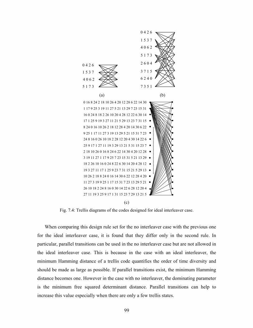
0 4 2 6

1 5 3 7

4 0 6 2

5 1 7 3

0 4 2 6

1 5 3 7

4 0 6 2

5 1 7 3

2 6 0 4

3 7 1 5

6 2 4 0

7 3 5 1 (a) (b)

0 16 8 24 2 18 10 26 4 20 12 28 6 22 14 30

1 17 9 25 3 19 11 27 5 21 13 29 7 23 15 31

16 0 24 8 18 2 26 10 20 4 28 12 22 6 30 14

17 1 25 9 19 3 27 11 21 5 29 13 23 7 31 15

8 24 0 16 10 26 2 18 12 28 4 20 14 30 6 22

24 8 16 0 26 10 18 2 28 12 20 4 30 14 22 6

2 18 10 26 0 16 8 24 6 22 14 30 4 20 12 28

18 2 26 10 16 0 24 8 22 6 30 14 20 4 28 12

10 26 2 18 8 24 0 16 14 30 6 22 12 28 4 20

26 10 18 2 24 8 16 0 30 14 22 6 28 12 20 4

9 25 1 17 11 27 3 19 13 29 5 21 15 31 7 23

25 9 17 1 27 11 19 3 29 13 21 5 31 15 23 7

3 19 11 27 1 17 9 25 7 23 15 31 5 21 13 29

19 3 27 11 17 1 25 9 23 7 31 15 21 5 29 13

11 27 3 19 9 25 1 17 15 31 7 23 13 29 5 21

27 11 19 3 25 9 17 1 31 15 23 7 29 13 21 5 (c)

Fig. 7.4: Trellis diagrams of the codes designed for ideal interleaver case.

When comparing this design rule set for the no interleaver case with the previous one

for the ideal interleaver case, it is found that they differ only in the second rule. In

particular, parallel transitions can be used in the no interleaver case but are not allowed in

the ideal interleaver case. This is because in the case with an ideal interleaver, the

minimum Hamming distance of a trellis code quantifies the order of time diversity and

should be made as large as possible. If parallel transitions exist, the minimum Hamming

distance becomes one. However in the case with no interleaver, the dominating parameter

is the minimum free squared determinant distance. Parallel transitions can help to

increase this value especially when there are only a few trellis states.

99

Two code examples based on the same signal constellation as before are given in this

subsection. The trellis diagrams are shown in Fig. 7.5. Both of the codes have parallel

transitions denoted by { , }. For code (a), the code rate is 2/3 with the spectral efficiency

R = 1 bit/s/Hz. It is not difficult to see that the error path within the parallel transitions

achieves the minimum free squared determinant distance of 4. In this case, the

equality in (7.16) holds. Hence, the actual coding advantage δ is also 4. With a coherent

receiver, its asymptotic coding gain over uncoded constellation G = ([1 1]; 4) with =

2 at the same spectral efficiency is expected to be 10 = 3.01 dB. For

code (b), the code rate is 4/5 with R = 2 bit/s/Hz. It is examined that the parameter

and δ are equal to 1.5999 and 1.7631, respectively, where the former is slightly smaller

than the latter. The asymptotic coding gain over uncoded constellation G = ([1 7]; 16)

with = 0.5858 at the same spectral efficiency is 4.78 dB when the receiver knows

CSI.

2freeD

2free10 D

2minD

2freeD

( 2min/log D )

2minD

{0,4} {2,6}

{1,5} {3,7}

{2,6} {0,4}

{3,7} {1,5}

{0,16} {2,18} {8,24} {10,26} {4,20} {6,22} {12,28} {14,30}

{1,17} {3,19} {9,25} {11,27} {5,21} {7,23} {13,29} {15,31}

{2,18} {0,16} {10,26} {8,24} {6,22} {4,20} {14,30} {12,28}

{3,19} {1,17} {11,27} {9,25} {7,23} {5,21} {15,31} {13,29}

{8,24} {10,26} {0,16} {2,18} {12,28} {14,30} {4,20} {6,22}

{10,26} {8,24} {2,18} {0,16} {14,30}{12,28} {6,22} {4,20}

{4,20} {6,22} {12,28} {14,30} {0,16} {2,18} {8,24} {10,26}

{6,22} {4,20} {14,30} {12,28} {2,18}{0,16} {10,26} {8,24}

{12,28} {14,30} {4,20} {6,22} {8,24} {10,26} {0,16} {2,18}

{14,30} {12,28} {6,22} {4,20} {10,26} {8,24} {2,18} {0,16}

{9,25} {11,27} {1,17} {3,19} {13,29} {15,31} {5,21} {7,21}

{11,27} {9,25} {3,19} {1,17} {15,31}{13,29} {7,23} {5,21}

{5,21} {7,23} {13,29} {15,31} {1,17} {3,19} {9,25} {11,27}

{7,23} {5,21} {15,31} {13,29} {3,19}{1,17} {11,27} {9,25}

{13,29} {15,31} {5,21} {7,23} {9,25} {11,27} {1,17} {3,19}

{15,31} {13,29} {7,23} {5,21} {11,27} {9,25} {3,19} {1,17} (a) (b)

Fig. 7.5: Trellis diagrams of the codes designed for no interleaver case: (a) rate 2/3 4-state with G

= ([1 3]; 8); (b) rate 4/5 16-state with G = ([1 7]; 32).

100


In Fig. 7.6 we provide the bit error rate (BER) performance of the two codes with R = 1

bit/s/Hz designed for the ideal interleaver case shown in Table 7.3 and Fig. 7.4. The

channel is modeled as flat Rayleigh fading with an ideal interleaver/deinterleaver. The

channel coefficients are kept constant within each time block and are not known to either

the transmitter or the receiver. The derived ML differential decoder (7.5) is employed.

For comparison, the BER performance of uncoded constellation G = ([1 1]; 4) at the same

spectral efficiency is also provided. Gray mapping is used from the binary information

bits to the elements in the constellation. As can be seen in this figure, a significant

improvement is observed. In particular, at a BER of 10-3 and with one receive antenna,

the 4-state code achieves around 5 dB gains compared with the uncoded case, while the

8-state code is seen to provide more than 6.5 dB improvement over the uncoded case.

When the number of receive antennas is increased to two, the improvement is not so

large, but a gain of 3~4 dB at a BER of 10-3 can still be achieved by these two codes.

For the code with R = 1 bit/s/Hz designed for the no interleaver case shown in

Fig.7.5(a), we first demonstrate its performance with direct transmission and coherent

receiver, and then show its performance with differential transmission and suboptimal

non-coherent receiver (7.12). This is done to confirm our statement in Section 7.2.2 that a

good TC-USTM also works well in the non-coherent case if an inner differential encoder

is employed. The channel is assumed to be constant during a frame of 100 transmission

time intervals, and an additional two time intervals are required to send an initial signal

matrix in the differential transmission case. As the errors caused by fading tend to occur

in bursts, frame error rate (FER) rather than BER is simulated.

Fig. 7.7 illustrates the results of direct transmissions with a coherent receiver for this

rate 2/3 4-state code. The results of the corresponding uncoded transmission at the same

spectral efficiency are given for comparison. It can be observed in Fig. 7.7 that there is

no diversity improvement but a coding gain of 3 dB over a wide range of FER is

achieved by this code, as expected, compared with the uncoded case at both one and two

receive antennas.

101

2 4 6 8 10 12 14 16 18 20 22 24

10−5

10−4

10−3

10−2

10−1

SNR [dB]

Bit

Err

or R

ate

(2,1) uncoded G=([1 1];4)(2,1) 4−state G=([1 3];8)(2,1) 8−state G=([1 3];8)(2,2) uncoded G=([1 1];4)(2,2) 4−state G=([1 3];8)(2,2) 8−state G=([1 3];8)

Fig. 7.6: BER of rate 2/3 4-state and 8-state G = ([1 3]; 8) TC-DUSTM compared with uncoded

G = ([1 1]; 4) DUSTM, ML differential decoder and ideal interleaver, R = 1 bit/s/Hz.

102

0 2 4 6 8 10 12 14 16 1810

−3

10−2

10−1

100

SNR [dB]

Fra

me

Err

or R

ate

(2,1) uncoded G=([1 1];4)(2,1) 4−state G=([1 3];8)(2,2) uncoded G=([1 1];4)(2,2) 4−state G=([1 3];8)

Fig. 7.7: FER of rate 2/3 4-state G = ([1 3]; 8) TC-USTM compared with uncoded G = ([1 1]; 4)

USTM, ML coherent decoder and no interleaver, frame length = 100, R = 1 bit/s/Hz.

The results of differential transmission with the non-coherent receiver are illustrated

in Fig. 7.8. The simulated coding gain over the uncoded system is about 2.4 dB at both

one and two receive antennas. 0.6 dB gain is lost compared with direct transmission and

coherent receiver. A comparison with Fig. 7.7 shows that the differentially non-coherent

results have a performance loss of 3.5 dB.

In Fig. 7.8 this code is also compared with the traditional TC-DPSK designed for

single transmit antenna. For a fair comparison, both the spectral efficiency and the trellis

state number are set the same. The TC-DPSK for R = 1 bit/s/Hz is constructed using the

rate 1/2 4-state convolutional code with Gray mapped QPSK. The antenna diversity gain

enhancement is obvious by the use of TC-DUSTM. This yields a substantial

improvement in FER especially when there is only one receive antenna.

103

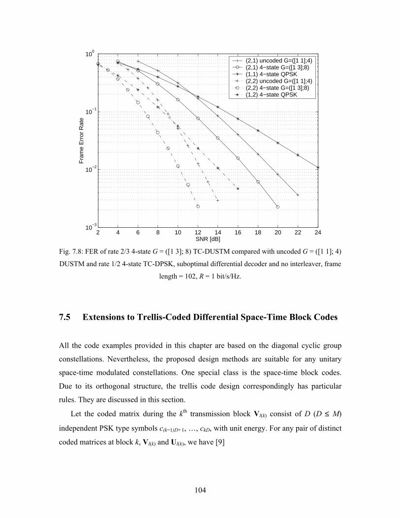
2 4 6 8 10 12 14 16 18 20 22 2410

−3

10−2

10−1

100

SNR [dB]

Fra

me

Err

or R

ate

(2,1) uncoded G=([1 1];4)(2,1) 4−state G=([1 3];8)(1,1) 4−state QPSK(2,2) uncoded G=([1 1];4)(2,2) 4−state G=([1 3];8)(1,2) 4−state QPSK

Fig. 7.8: FER of rate 2/3 4-state G = ([1 3]; 8) TC-DUSTM compared with uncoded G = ([1 1]; 4)

DUSTM and rate 1/2 4-state TC-DPSK, suboptimal differential decoder and no interleaver, frame

length = 102, R = 1 bit/s/Hz.

7.5 Extensions to Trellis-Coded Differential Space-Time Block Codes

All the code examples provided in this chapter are based on the diagonal cyclic group

constellations. Nevertheless, the proposed design methods are suitable for any unitary

space-time modulated constellations. One special class is the space-time block codes.

Due to its orthogonal structure, the trellis code design correspondingly has particular

rules. They are discussed in this section.

Let the coded matrix during the kth transmission block Vl(k) consist of D (D ≤ M)

independent PSK type symbols c(k−1)D+1, …, ckD, with unit energy. For any pair of distinct

coded matrices at block k, Vl(k) and Ul(k), we have [9]

104

( ) ( ) M

D

iiDkiDkklkl

Hklkl ec

DIUVUV ∑

=+−+− −=−−

1

2)1()1()()()()(

1 , (7.19)

where e(k−1)D+i , i = 1, …, D, are the symbols contained in Ul(k).

We first consider the case without an interleaver. The coding advantage δ in (7.15)

and the minimum free squared determinant distance in (19) are equal because of the

orthogonality shown in (7.19). We rewrite (7.15) as

2freeD

∑∑∑∈≠∈ =

+−+−≠−=−=

ςηδ

ttt

k

D

iiDkiDk ec

Dec

D2

1

2)1()1(

1min1minecUV

(7.20)

where c = {ct} and e = {et} are the symbol sequences contained in the coded matrix

sequences V and U, respectively, and ς is the set of all t that ct differs from et. Using

(7.20), the design criterion becomes maximizing the minimum free squared Euclidean

distance between any distinct symbol sequence pairs. Therefore, using the conventional

set-partition method, we simply map the binary coded bits to the symbols ct directly,

rather than the matrix Vl(k).

Next, we consider the case when an ideal interleaver/deinterleaver is used. We rewrite

the PWEP in (7.9) as

( ) ∏ ∑∈

−

=+−+−

−

−

≤→

ησρ

k

MND

iiDkiDk

vMN

ecD

P1

2)1()1(2

18

UV .

We further propose a layered structure for this system. The information bits are divided

into D substreams (or layers), each of which is then encoded using an individual

component trellis code with outputs mapped to symbols c(k-1)D+i at the kth time block for

the ith layer. All the component codes are set to be identical for simplicity and have the

minimum Hamming distance of v. Then, the whole system achieves vMN order of

combined antenna and time diversity. At the receiver, since every coded data symbol is

decoupled without the loss of any information, all the component codes can be decoded

individually. To better understand the benefit of having a layered structure, we compare

its decoding complexity with that of the general joint coding structure. The decoding

complexity is measured in the same way as introduced in Section 7.2.1, i.e., the average

number of branch metric calculations for each info bit through the soft-decision Viterbi

decoder. Let the spectral efficiency R be m / M bit/s/Hz and each component code has the

105

minimum trellis states to ensure the minimum Hamming distance is v. Then the

complexity of the layered structure is

Dmv /)1(2 −

stateper branches

/2 Dm × × layers

/ = statesmin

/)1(2 Dmv− Dbits info

mm

D Dmv /2 . (7.21)

However, at the same spectral efficiency and diversity order, the complexity of the joint

coding structure has to be

stateper branches2m × / =

statesmin

)1(2 −vm

bits infom

m

mv2 . (7.22)

Comparing (7.21) with (7.22), it can be observed that the proposed layered structure

significantly reduces the decoding complexity. As an example, let M = 2 (D = 2 in this

case), R = 4 bit/s/Hz and v = 2, the layered strategy has a complexity of 26 = 64 branch

metric calculations per info bit, while the joint coding strategy has that of 213 = 8192

branch metric calculations per info bit.

7.6 Summary

In this chapter we proposed trellis-coded differential unitary space-time modulation. No

channel estimation is required in this scheme. Therefore, it reduces the receiver

complexity and relaxes the design requirement on the pilot signals. We derived decision

metrics for differential decoding and proposed design criteria for the trellis codes. We

also described a general set-partition method for unitary space-time modulated

constellations based on their determinant distance profile, and code constructions for

Ungerboeck type trellis codes. Several code examples, based on diagonal cyclic group

constellations, were provided. Simulation results exhibited excellent performance with

computationally efficient non-coherent receivers.

We also considered the extensions to trellis-coded differential space-time block

codes. Therein, the decoupling property retained by space-time block codes allows

efficient and simple encoding and decoding structures.

106

Chapter 8

CONCLUSION AND FURTHER WORK

In this chapter we give some concluding remarks on this work and discuss several directions for further work.

8.1 Conclusion

In this thesis, we have studied the design of space-time transmission techniques mainly

from the coding perspective in multiple-antenna wireless communication systems. The

main contributions of this thesis are summarized as follows.

We proposed in Chapter 3 a set of improved design criteria for space-time trellis-

coded modulation taking care of different operating SNRs in quasi-static channel

environments. We essentially divided the SNR into three regions: high, moderate

and low SNR regions and proposed individual design criteria for each of them. It

was shown that the full-rank criterion is no longer necessary at both moderate

and low SNRs. It was also shown that the minimum Euclidean distance of a code

is the dominating factor at low SNR. Based on these improved design criteria, we

provided several space-time trellis code examples using two transmit antennas

via computer search, which are expected to work optimally at moderate SNR

regions. Simulation results demonstrated that they outperform the codes based on

the traditional criteria over a wide SNR range.

To avoid the prohibitively large time complexity of searching for good space-

time trellis codes with a larger number of transmit antennas and high modulation

level, we proposed in Chapter 4 diagonal block space-time coding, a systematic

code structure. The key of this approach is to separate the traditional design

method into two parts. It first encodes the information symbols by a one-

dimensional nonbinary block code, and then transmit the coded symbols

diagonally across the space-time grid. It was shown that this scheme can achieve

107

full transmit diversity and good coding advantage and, hence, is particularly

suitable for high SNR. This coding approach is suitable for an arbitrary number

of transmit antennas with arbitrary signal constellations. Some code examples

with 2 ~ 6 bit/s/Hz spectral efficiency and 2 ~ 6 transmit antennas were provided

and demonstrated excellent performance in computer simulation. Though it was

proposed for flat fading channels, this coding scheme can be easily extended to

frequency-selective fading to achieve the maximum possible combined antenna

and frequency diversity.

We presented in Chapter 5 the generalized layered space-time architecture which

provides a tradeoff between diversity order and transmission rate. This

architecture can be viewed as a compromise between traditional space-time

coding and traditional layered space-time architecture and both of them appear as

an extreme case of GLST. A number of important aspects, including signal-to-

antenna mapping, decoding order and power allocation were discussed.

Moreover, a low complexity iterative decoding algorithm was proposed that

efficiently exploits full receive diversity and, hence, dramatically improves the

overall system performance.

We proposed in Chapter 6 differential space-time block codes that do not require

channel knowledge for decoding at the receiver. This differential scheme allows

multiple-amplitude modulation for uncoded data symbols and can be designed

for any number of transmit antennas where orthogonal space-time block code

with square codeword matrices exists. We also did a comparison between this

scheme and DUSTM with diagonal cyclic group constellations, and significant

advantages have been demonstrated in both decoding complexity and error

performance.

We proposed in Chapter 7 the design of outer trellis channel coding in front of

the general differential unitary space-time modulation to further enhance the

system performance without requiring channel knowledge at the receiver. It

brought considerable coding gain and possibly diversity gain in a time-varying

fading environment if a matrix-wise interleaver is applied. It also demonstrated

108

significant performance improvement at the same complexity over traditional

coded differential scheme with only a single transmit antenna.

8.2 Further Work

There are several possible directions that can follow the work done in this thesis.

Rate-diversity space-time codes

Our previously studied generalized layered space-time architecture is just at the early

stage of a new research direction, that is, rate-diversity space-time codes. As a matter of

fact, the tradeoff between rate and diversity only exists when the modulation for the

transmitted symbols is fixed [8]. Recent efforts in [68, 69, 71, 73] revealed that, if (linear)

precoding or constellation rotation in the complex field is applied, the tradeoff

disappears. This is ensured by the information-theoretic study in [72]. Nevertheless, the

techniques on this “rate-diversity” topic are far from mature and there is still a lot of

research potential. For example, the peak-to-average power ratio, the resolution of

complex numbers, and the joint design and decoding with outer channel coding are the

issues.

Higher-rate trellis-coded differential space-time modulation

Similar to the traditional TCM concept, our previously proposed TC-DUSTM requires

expansion on the space-time modulation in order to achieve the same spectral efficiency

as uncoded systems. It may also be possible to achieve the same spectral efficiency

without expansion due to the additional degree of freedom introduced by multiple

transmit antennas. In fact, a superset technique [20, 21, 22] has already been applied in

the design of concatenated STBC with TCM to achieve similar objectives. It is, therefore,

expected that a similar technique can be developed for our TC-DUSTM to avoid

constellation expansion and, hence, be more spectrally efficient. The detailed superset

technique, the set-partition of unitary space-time modulation, and the design of trellis

codes need to be carefully addressed.

109

MIMO in future wireless networks

The MIMO systems we considered so far are point-to-point wireless links with flat fading

channels. When a multi-access or broadcasting channel is considered, MIMO can provide

interference suppression gain besides diversity and spectral efficiency gain. In that case,

the development of combined signal processing and space-time coding schemes to exploit

these gains is necessary. In addition, when a broadband wireless connection is

considered, it is necessary to extend this work to frequency-selective channels.

110

Bibliography

[1] G. J. Foschini and M. J. Gans, “On limits of wireless communications in a fading

environment when using multiple antennas,” Wireless Personal Communications,

vol.6, no.3, March 1998.

[2] I. E. Telatar, “Capacity of multi-antenna Guassian Channels,” European Trans. on

Telecom., vol.10, no.6, Nov/Dec 1999.

[3] G. J. Foschini, “Layered space-time architecture for wireless communication is a

fading environment when using multiple antennas,” Bell Labs Technical Journal,

vol.1, no.2, Autumn 1996.

[4] G. D. Golden, C. J. Foschini, R. A. Valenzuela and P. W. Wolniansky, “Detection

algorithm and initial laboratory results using V-BLAST space-time communication

architecture,” Electronics Letters, vol.35, no.1, Jan. 1999.

[5] P. W. Wolniansky, G. J. Foschini, G. D. Golden and R. A. Yalenzuela,“V-BLAST:

an architecture for realizing very high data rates over the rich-scattering wireless

channel,” Proc.1998 URSI International Symposium on Signals, Systems, and

Electronics, New York, 1998.

[6] G. J. Foschini, G. D. Golden, R. A. Valenzuela, and P. W. Wolniansky, “Simplified

processing for high spectral efficiency wireless communications employing multi-

element arrays,” IEEE Journal on Selected Areas in Comm., vol.17, no.11, Nov.

1999.

[7] J. C. Guey, M. P. Fitz, M. R. Bell and W. Y. Kuo, “Signal design for transmitter

diversity wireless communication systems over Rayleigh fading channels”, IEEE

Trans. on Comm., vol. 47, no. 4, pp. 527-537, April 1999.

[8] V. Tarokh, N. Seshadri, and A. R. Calderbank, “Space-time codes for high data rate

wireless communication: performance criterion and code construction,” IEEE

Trans. on Infor. Theory, vol.44, no.2, March 1998.

111

[9] V. Tarokh, H. Jafarkhani, and A. R. Calderbank, “Space-time block codes from

orthogonal designs,” IEEE Trans. on Infor. Theory, vol.45, no.5, July 1999.

[10] V. Tarokh, H. Jafarkhani, and A. R. Calderbank, “Space-time block coding for

wireless communications: performance results,” IEEE Journal on Selected Areas in

Commu., vol. 17, no. 3, March 1999.

[11] S. M. Alamouti, “A simple transmit diversity technique for wireless

communications,” IEEE Journal on Selected Areas in Comm., vol.16, no.8, Oct.

1998.

[12] G. Ganesan and P. Stoica, “Space-time diversity using orthogonal and amicable

orthogonal designs”, in Proc. Int. Conf. Acoustics, Speech, Signal Processing

(ICASSP), Istanbul, Turkey, 2000.

[13] G. Ganesan and P. Stoica, “Space-time block codes: A maximum SNR approach”,

IEEE Trans. on Infor. Theory, vol. 47, no. 4, pp. 1650-1656, May 2001.

[14] H. Jafarkhani, “A quasi-orthogonal space-time block code”, IEEE Trans. on

Commu., vol. 49, no. 1, pp. 1-4, Jan. 2001.

[15] O. Tirkkonen and A. Hottinen, “Complex space-time block codes for four Tx

antennas”, in Proc. GLOBECOM’00, 2000.

[16] O. Tirkkonen, A. Boariu, and A. Hottinen, “Minimal non-orthogonality rate 1 space-

time block codes for 3+ Tx antennas”, in Proc. IEEE 6th Symp. On Spread-Spectrum

Tech. & Application, New Jersey, USA, Sept. 6~8, 2000.

[17] W. Su and X.-G. Xia, “Quasi-orthogonal space-time block codes with full

diversity”, in Proc. IEEE Global Telecom. Conference (GLOBECOM’02), 2002.

[18] Il-Min Kim and V. Tarokh, “Variable-rate space-time block codes in M-ary PSK

systems”, IEEE Journal on Selected Areas in Comm., vol. 21, no. 3, pp. 362-373,

April 2003.

[19] V. Tarokh, A. Naguib, N. Seshadri, and A. R. Calderbank, “Combined array

processing and space-time coding,” IEEE Trans. on Infor. Theory, vol.45, no.4, May

1999.

112

[20] S. Siwamogsatam and M. Fitz, “Improved high rate space-time codes via

orthogonality and set partitioning”, in Proc. WCNC’02, 2002.

[21] S. Siwamogsatam and M. Fitz, “Improved high rate space-time TCM via

concatenation of expanded orthogonal block codes and MTCM”, in Proc ICC’02,

2002.

[22] H. Jafarkhani and N. Seshadri, “Super-orthogonal space-time trellis codes”, IEEE

Trans. on Infor. Theory, vol. 49, no. 4, pp. 937-950, April 2003.

[23] T. H. Liew, J. Pliquett, B. L. Yeap, L.-L. Yang, and L. Hanzo, “Comparative study

of space-time block codes and various concatenated turbo coding schemes”, in Proc.

IEEE International. Symp. on Personal, Indoor and Mobile Radio Comm.

(PIMRC’00), 2000.

[24] G. Bauch, “Concatenation of space-time block codes and ‘turbo’-TCM”, in Proc.

ICC’99, 1999.

[25] S. Baro, G. Bauch and A. Hansmann, “Improved codes for space-time trellis coded

modulation,” IEEE Comm. Letters, vol. 4, no. 1, Jan. 2000.

[26] Q. Yan and R. S. Blum, “Optimum space-time convolutional codes,” in Proc.

WCNC, Sept. 2000.

[27] Q. Yan and R. S. Blum, “Improved space-time convolutional codes for quasi-static

slow fading channels”, IEEE Trans. on Wireless Comm., vol. 1, no. 4, pp. 563-571,

Oct. 2002.

[28] X. Lin and R. S. Blum, “Systematic design of space-time codes employing multiple

trellis coded modulation”, IEEE Trans. on Comm., vol. 50, no. 4, pp. 608-615, April

2002.

[29] E. Biglieri, G. Taricco, and A. Tulino, “Performance of space-time codes for a large

number of antennas”, IEEE Trans. on Infor. Theory, vol. 48, no. 7, 1794-1803, July

2002.

[30] Z. Cheng, J. Yuan, and B. Vucetic, “An improved space-time trellis coded

modulation scheme on slow Rayleigh fading channels”, in Proc. ICC 2001.

113

[31] Z. Chen, B. S. Vucetic, J. Yuan and K. L. Lo, “Space-time trellis codes for 4-PSK

with three and four transmit antennas in quasi-static flat fading channels”, IEEE

Comm. Letters, vol. 6, no. 2, pp. 67-69, Feb. 2002.

[32] Z. Chen, B. S. Vucetic, K. L. Lo and J. Yuan, “Space-time trellis codes for 8-PSK

with two, three and four transmit antennas in quasi-static flat fading channels”,

Electronics Letters, vol. 38, no. 10, pp. 462-464, May 2002.

[33] Z. Chen, B. S. Vucetic, J. Yuan and K. L. Lo, “Space-time trellis codes with two,

three and four transmit antennas in quasi-static flat fading channels”, in Proc.

ICC’02, May 2002.

[34] H. El Gamal, A. R. Hammons, Jr., “On the design and performance of algebraic

space-time codes for BPSK and QPSK modulation”, IEEE Trans. on Comm., vol.

50, no. 6, pp. 907-913, June 2002.

[35] A. R. Hammons, Jr. and H. El Gamal, “On the theory of space-time codes for PSK

modulation”, IEEE Trans. on Infor. Theory, vol. 46, no. 2, pp. 524-542, March

2000.

[36] D. M. Ionescu, “New results on space-time code design criteria,” in Proc.

WCNC’99, Sept. 1999.

[37] R. van Nee, A. van Zelst and G. Awater, “Maximum likelihood decoding in a space

division multiplexing system,” in Proc. IEEE VTC 2000, Tokyo, Japan, May 2000.

[38] Da-shan Shiu, “Iterative decoding for layered space-time codes,” in Proc. IEEE ICC

2000, New Orleans, Louisiana, USA, June 2000.

[39] S. L. Ariyavisitakul, “Turbo space-time processing to improve wireless channel

capacity,” in Proc. IEEE ICC 2000, New Orleans, Louisiana, USA, June 2000.

[40] S. Baro, G. Bauch, A. Pavlic, and A. Semmler, “Improving BLAST performance

using space-time block codes and turbo decoding,” in Proc GLOBECOM’00, 2000.

[41] Da-shan Shiu and J. M. Kahn, “Layered space-time codes for wireless

communications using multiple transmit antennas,” in Proc. IEEE ICC ’99, 1999.

114

[42] B. Hassibi, “An efficient square-root algorithm for BLAST”, in Proc. Acoustics,

Speech, and Signal Processing (ICAPP’00), 2000.

[43] N. Seshadri and J. Winters, “Two signaling schemes for improving the error

performance of frequency-division duplex (FDD) transmission systems using

transmitter antenna diversity”, in Proc. VTC’93, 1993.

[44] A. Wittneben, “A new bandwidth efficient transmit antenna modulation diversity

scheme for linear digital modulation”, in Proc. ICC’ 93, 1993.

[45] J. H. Winters, “The diversity gain of transmit diversity in wireless systems with

Raleigh fading”, IEEE Trans. on Vehicular Technology, vol. 47, no. 1, pp. 119-123,

Feb. 1998.

[46] S. Li, X. Tao, W. Wang, P. Zhang, and C. Han, “Generalized delay diversity code: a

simple and powerful space-time coding scheme”, in Proc. International Conference

on Communication Technology, 2000.

[47] Z. Safar and K. J. R. Liu, “Systematic design of space-time trellis codes for diversity

and coding advantage”, EURASIP Journal on Applied Signal Processing, pp. 221-

235, March 2002.

[48] A. Matache, R. D. Wesel and J. Shi, “Trellis coding for diagonally layered space-

time systems”, in Proc. ICC’02, May 2002.

[49] G. Caire and G. Colvalope, “On space-time coding for quasi-static multiple-antenna

channels”, in Proc. Globecom’01, San Antonio TX, Nov. 2001.

[50] D. Gore, S. Sandhu and A. Paulraj, “Delay diversity code for frequency selective

channels”, Electronics Letters, vol. 37, no. 20, Sept. 2001.

[51] T. L. Marzetta and B. M. Hochwald, “Capacity of a mobile multiple-antenna

communication link in Rayleigh flat fading,” IEEE Trans. on Infor. Theory, vol. 45,

no. 1, Jan. 1999.

[52] L. Zheng and D. N. C. Tse, “Communication on the Grassmann manifold: A

geometric approach to the noncoherent multiple-antenna channel”, IEEE Tran. on

Infor. Theory, vol. 48, no. 2, pp. 359-383. Feb. 2002.

115

[53] B. M. Hochwald and T. L. Marzetta, “Unitary space-time modulation for multiple-

antenna communications in Rayleigh flat fading”, IEEE Trans. on Infor. Theory,

vol, 46, no. 2, pp. 543-564, March 2000.

[54] B. M. Hochwald,T. L. Marzetta, T. J. Richardson, W. Sweldens, and R. Urbanke,

“Systematic design of unitary space-time constellations”, IEEE Trans. on Infor.

Theory, vol. 46, no. 6, pp. 1962 -1973, Sept. 2000.

[55] B. Hassibi, B. W.Hochwald, A. Shokrollahi and W. Sweldens, “Representation

theory for high-rate multiple-antenna code design,” IEEE Trans. on Infor. Theory,

vol. 47, no. 6, pp. 2335-2367, Sept. 2001.

[56] B. L. Hughes, “Differential space-time modulation,” IEEE Trans. on Infor. Theory,

vol. 46, no. 7, Nov. 2000.

[57] B. M. Hochwald and W. Sweldens, “Differential unitary space-time modulation,”

IEEE Trans. on Comm., vol. 48, no. 12, Dec. 2000.

[58] V. Tarokh and H. Jafarkhani, “A differential detection scheme for transmit

diversity,” IEEE Journal on Selected Areas in Comm., vol. 18, no. 7, July 2000.

[59] G. Ganesan and P. Stoica, “Differential modulation using space-time block codes”,

IEEE Signal Processing Letters, vol. 9, no. 2, pp. 57-60, Feb. 2002.

[60] E. G. Larsson, P. Stoica and J. Li, “On maximum-likelihood detection and decoding

for space-time coding systems”, IEEE Trans. on Signal Processing, vol. 50, no. 4,

pp. 937-944, April 2002.

[61] J. Wang, M. P. Fitz, and K. Yao, “Differential unitary space-time modulation for a

large number of receive antennas”, in Proc. 36th Asilomar Conference on Signals,

Systems and Computers, 2002.

[62] X.-B. Liang and X.-G. Xia, “Unitary signal constellations for differential space-time

modulation with two transmit antennas: parametric codes, optimal designs, and

bounds”, IEEE Trans. on Infor. Theory, vol. 48, no. 8, pp. 2291-2322, Aug. 2002.

[63] X.-G. Xia, “Differentially en/decoded orthogonal space-time block codes with

APSK signals”, IEEE Comm. Letters, vol. 6, no. 4, pp. 150-152, April 2002.

116

[64] D. Divsalar and M. K. Simon, “Multiple-symbol differential detection of MPSK”,

IEEE Trans. on Comm., vol. 38, no. 3, pp. 300-308, March 1990.

[65] J. B. Anderson and S. Mohan, “Sequential decoding algorithms: A survey and cost

analysis”, IEEE Trans. on Comm., vol. 32, pp. 169-176, Feb. 1984.

[66] E. Viterbo, J. Boutros, “A universal lattice code decoder for fading channels”, IEEE

Trans. on Infor. Theory, vol. 45, no. 5, pp. 1639-1642, July 1999.

[67] O. Damen, A. Chkeif and J-C Belfiore, “Lattice code decoder for space-time codes”,

IEEE Commn. Letters, vol. 4, no. 5, pp. 161-163, May 2000.

[68] B. Hassibi and B. M. Hochwald, “High-rate codes that are linear in space and time”,

IEEE Trans. on Infor. Theory, vol. 48, no. 7, pp. 1804-1824, July 2002.

[69] R. W. Heath, Jr and A. J. Paulraj, “Linear dispersion codes for MIMO systems

based on frame theory”, IEEE Trans. on Signal Proecessing, vol. 50, no. 10, Oct.

2002.

[70] M. O. Damen, K. Abed-Meraim, and J-C. Belfiore, “Diagonal algebraic space-time

block codes”, IEEE Trans. on Infor. Theory, vol. 48, no. 3, pp. 628-636, March

2002.

[71] M. O. Damen, A. Tewfik, and J.-C. Belfiore, “A construction of a space-time code

based on number theory”, IEEE Trans. on Infor. Theory, vol. 48, no. 3, pp. 753-760,

March 2002.

[72] L. Zheng and D. N. C. Tse, “Divesity and multiplexing: a fundamental tradeoff in

multiple antenna channels”, IEEE Trans. on Infor. Theory, vol. 49, no. 5, pp. 1073-

1096, May 2003.

[73] H. El Gamal and M. O. Damen, “Universal space-time coding”, IEEE Trans. on

Infor. Theory, vol. 49, no. 5, pp. 1097-1119, May 2003.

[74] R. A. Horn and C. R. Johnson, Matrix Analysis, Cambridge University Press 1985.

[75] G. L. Nemhauser, A. H. G. Rinnooy Kan and M. J. Todd, Optimization, North-

Holland, Amsterdam, 1989.

117

[76] E. Biglieri, D. Divsalar, P. J. McLane and M. K. Simon, Introduction to trellis-

coded modulation with applications, Macmillan Publishing Company, 1991.

[77] T. S. Rappaport, Wireless Communications Principles & Practice, Prentice Hall,

Inc., a Simon & Schuster Company, 1996.

[78] J. G. Proakis, Digital Communications, Third Edition, McGraw-Hill, Inc., 1995.

118

Documents

Space-Time Coding Schemes for Wireless Communications over ...iwct.sjtu.edu.cn/personal/mxtao/paper/mxtaoPhDthesis.pdf · Space-Time Coding Schemes for Wireless Communications over