Data-Driven Revenue Management

Data-Driven Revenue Management

by

Joline Ann Villaranda Uichanco

Submitted to the School of Engineeringin partial fulfillment of the requirements for the degree of

Master of Science in Computation for Design and Optimization

at the

MASSACHUSETTS INSTITUTE OF TECHNOLOGY

September 2007

© Massachusetts Institute of Technology 2007. All rights reserved.

A uthor .......................... ...... :..........................IU

hc ool of Engineering

September 17, 2007

Certified by.............. ......... .. ..........................J Retsef Levi

Robert N. Noyce Career Development Professor, Assistant Professorof Management

Thesis Supervisor

Certified by ................ ... .......... ....................Georgia Perakis

J. Spencer Standish Career Development Associate Professor ofOperations Research

] IL Thesis Supervisor

Accepted by..... ............. T... ... .... M"g .1 ..

SJaime Peraire

MASSACHUSETTS INSTrTUTE.OF TECHNOLOGY

SEP 2 7 2007

LIBRARIES

Co-director, Computation for Design and Optimization Program

A~RCHWES~C

Data-Driven Revenue Management

by

Joline Ann Villaranda Uichanco

Submitted to the School of Engineeringon September 17, 2007, in partial fulfillment of the

requirements for the degree ofMaster of Science in Computation for Design and Optimization

Abstract

In this thesis, we consider the classical newsvendor model and various importantextensions. We do not assume that the demand distribution is known, rather theonly information available is a set of independent samples drawn from the demanddistribution. In particular, the variants of the model we consider are: the classicalprofit-maximization newsvendor model, the risk-averse newsvendor model and theprice-setting newsvendor model. If the explicit demand distribution is known, thenthe exact solutions to these models can be found either analytically or numericallyvia simulation methods. However, in most real-life settings, the demand distributionis not available, and usually there is only historical demand data from past periods.Thus, data-driven approaches are appealing in solving these problems.

In this thesis, we evaluate the theoretical and empirical performance of nonpara-metric and parametric approaches for solving the variants of the newsvendor model as-suming partial information on the distribution. For the classical profit-maximizationnewsvendor model and the risk-averse newsvendor model we describe general non-parametric approaches that do not make any prior assumption on the true demanddistribution. We extend and significantly improve previous theoretical bounds on thenumber of samples required to guarantee with high probability that the data-drivenapproach provides a near-optimal solution. By near-optimal we mean that the ap-proximate solution performs arbitrarily close to the optimal solution that is computedwith respect to the true demand distributions. For the price-setting newsvendor prob-lem, we analyze a previously proposed simulation-based approach for a linear-additivedemand model, and again derive bounds on the number of samples required to en-sure that the simulation-based approach provides a near-optimal solution. We alsoperform computational experiments to analyze the empirical performance of thesedata-driven approaches.

Thesis Supervisor: Retsef LeviTitle: Robert N. Noyce Career Development Professor, Assistant Professor of Man-agement

Thesis Supervisor: Georgia PerakisTitle: J. Spencer Standish Career Development Associate Professor of OperationsResearch

Acknowledgments

I would like to thank first and foremost my supervisors, Prof. Retsef Levi and Prof.

Georgia Perakis. Without them pushing me to do my best, this thesis wouldn't have

been possible. Our discussions have been extremely enjoyable and I learned a lot

about the joys and pains of research from them. Words cannot express the gratitude

I feel for the time and effort they put in each week to supervise my work. They

have both been my research supervisors, my technical writing teachers and my career

advisors. I am truly honored to have worked under them.

I would also like to acknowledge my fellow SMA students. We finally reached the

finish line.

My thanks and appreciation go out to my mother and to my brother who are

always supporting me. And to Simon for his patience over the last seven months.

Contents

1 Introduction

2 Data-Driven Approach to the Newsvendor Problem with Exogenous

Price

2.1 The Profit-Maximizing Newsvendor Model ...............

2.1.1 Problem Formulation .......................

2.1.2 Optimal Solution .........................

2.2 Sample Average Approximation . . . . . . . . . . . . . . . . . . . . .

2.3 Relative Error of the Regret of the Optimal Solution to the SAA Coun-

terpart . . . . . . . . . . . . . . . . . . . . . . . . . . . . . . . . . . .

2.4 The Newsvendor Model with Risk Preferences . . . . . . . . . . . . .

3 Numerical Results for the Data-Driven Newsvendor Problem with

Exogenous Price

3.1 M ethodology ........ .... ............ ... .. ..

3.2 Results and Discussion ..........................

4 Data-Driven Approach to the Price-Setting Newsvendor Problem

4.1 The Price-Setting Newsvendor Model . . . . . . . . . . . . . . . . . .


4.1.2 Optimality Conditions . . . . . . . . . . . . . . . . . . . . . .

4.2 Simulation-Based Procedure .......................


19

24

24

26

27

28

45

59

60

62

69

72

72

74

77

78

4.3 Relative Error of the Regret of the Solution to the Simulation-Based

Procedure ...... ............. ............. 79

4.3.1 Accuracy of the Regret of a First-Order Approximate Policy . 81

4.3.2 Sample Size to Ensure First-Order Accuracy of the Solution to

the Simulation-Based Procedure ................. 90

5 Numerical Results for the Data-Driven Price-Setting Newsvendor

Problem 97

5.1 Methodology ................... .......... .. 98

5.2 Results and Discussion ................... ....... 100

A Figures 105

List of Figures

2-1 Illustration of a cumulative distribution function, F, and distribution

function, F, and the quantiles ql and q2 . . . . . . . . . . . . . . . . . 36

2-2 Comparison of bounds implied by Hoeffding, and Bernstein for the

maximization variant of the newsvendor problem as a function of the

accuracy rate, for w = 0.01,0.05 ...................... 41

2-3 Comparison of bounds implied by Hoeffding, and Bernstein for the

maximization variant of the newsvendor problem as a function of the

accuracy rate, for w = 0.2,0.4 ....................... 42

2-4 Plot of regions of w = min (1 - A, A) for which the Hoeffding or the

Bernstein bound is tighter, for various accuracy rates, a. The y-axis is

in logarithmic scale ............................. 44

2-5 Comparison of bounds for the case of trimming and without trimming

(trimming factor 0=0.05) as a function of the accuracy level a. .... . 57

2-6 Plot of the bounds for for the required number of samples in the trim-

ming case as a function of the trimming factor p. ............ 58

4-1 Illustration of h(c) for the case when 1RN < p**. .............. 84

A-1 The sample average of the error of the SAA order quantity as a function

of the critical fractile A. ......................... 106

A-2 The accuracy level achieved by the sample average expected profit and

the sample average regret of the SAA order quantity as a function of

the critical fractile A for various distributions. . ............. 107



the mean p of the uniform distribution. .. ............... 108



the mean p of the normal distribution. . ................. 109



the standard deviation a of the normal distribution. .......... 110



the mean 1t of the exponential distribution. . .............. 111



the parameter k of the Pareto distribution. . ............. . 112

A-8 The relative error of the regret achieved by the minimax regret or-

der quantity and the SAA order quantity for the uniform and normal

distribution. ................... ............ .. 113

A-9 The relative error of the regret achieved by the minimax regret order

quantity and the SAA order quantity for the exponential and Poisson

distribution. ................... ............. 114

A-10 The relative error of the regret achieved by the parameter-estimation

order quantity and the SAA order quantity for the uniform and Pareto

distribution ......... . ............ 115

A-11 The relative error of the regret achieved by the parameter-estimation

order quantity and the SAA order quantity for the exponential and

Poisson distribution. ................... ........ 116



the unit cost c ....... ....................... 117



the zero-price demand a........................... 118



the price-sensitivity parameter b. . .................. . 119



the mean p of the uniform distribution. . ............. . . . 120



the mean p of the exponential distribution. . ............... 121



the mean p of the normal distribution. . ................. 122



the standard deviation a of the normal distribution. . ........ . 123



the parameter k of the Pareto distribution. . ............... 124

List of Tables

3.1 Theoretical and empirical confidence levels for various accuracy lev-

els of the solution to the SAA counterpart of the profit-maximizing

newsvendor with critical fractile A = 0.5 . ............... 63

3.2 Theoretical and empirical confidence levels for various accuracy lev-

els of the solution to the SAA counterpart of the profit-maximizing

newsvendor with critical fractile A = 0.9 . ............... 64

Chapter 1

Introduction

In this thesis, we address several important variants of the classical newsvendor model,

but under the assumption that the explicit demand distribution is not known. Rather,

the only information available is a set of independent samples drawn from the true

demand distribution. In particular, we consider three variants of the newsvendor

model: the classical profit-maximization newsvendor model, the newsvendor model

with risk preferences and the price-setting newsvendor model.

The classical profit-maximization model is a problem of matching supply and de-

mand where the supply must be chosen before observing the demand. Demand is

stochastic and the market parameters (i.e., price) are exogenous. In the classical

model, the firm is risk-neutral and chooses an optimal ordering quantity that maxi-

mizes its expected profit with respect to the full demand distribution. An extension

of the classical model that incorporates risk preferences of a firm is the risk-averse

newsvendor model which has been considered by Bertsimas and Thiele [5]. In this

variant, the goal is to maximize the expected profit over a natural set of worst-case

scenarios of the demand defined by the event that the demand is less than some spec-

ified quantile. Another extension is the price-setting newsvendor model. This model

apart from ordering decisions also incorporates pricing decisions. Under this model,

the demand is stochastic and a function of price, and the firm decides simultaneously

on the price and the supply level.

If the demand distribution is known explicitly, the exact solutions to these models

can be found either analytically or numerically via simulation methods. However,

in real-life settings, the explicit demand distribution is not known. Typically, partial

information on the demand is available from historical data or from simulations. Data-

driven approaches can thus be used to solve the model under partial information. It is

of interest to analyze the theoretical and empirical performance of these data-driven

approaches.

We discuss a nonparametric approach for solving the classical profit-maximization

newsvendor model that makes use of observed samples of the demand without any

assumptions on the true demand distribution. Levi, Roundy and Shmoys [24] consider

a cost-minimization newsvendor variant and derive bounds on the number of samples

required to ensure with high probability a good quality solution to the data-driven

approach. We extend the results to the profit-maximization variant, and in fact

significantly improve these bounds.

Bertsimas and Thiele [5] introduce a nonparametric data-driven approach based

on one-sided trimming to solve the risk-averse newsvendor problem with partial in-

formation on the demand. We provide a novel analysis regarding the number of

samples required to ensure that the data-driven one-sided trimming method provides

a near-optimal solution with high probability.

For the price-setting newsvendor problem, Zhan and Shen [421 propose a simulation-

based approach for a particular (i.e. linear-additive) form of the demand-price relation

assuming that the parameters are known. The approach uses observed samples of the

random component of the demand with only mild assumptions on its true distri-

bution. By imposing additional assumptions on the distribution, we again obtain

worst-case bounds on number of samples required for the simulation-based approach

to provide a good quality solution with high probability.

Finally, through computational experiments, we verify the empirical performance

of these data-driven approaches.

This thesis is structured as follows. In Chapter 2, we consider the classical

newsvendor problem under imperfect information. We describe and analyze a non-

parametric approach to the classical newsvendor problem. We also describe the

newsvendor problem with risk preferences and establish a connection between ac-

curacy and the sample size of the one-sided trimming approach to the risk-averse

newsvendor problem. In Chapter 3, we perform numerical experiments to evaluate

the performance of the data-driven approach for the classical newsvendor problem

under different concrete scenarios. We also compare its performance against other

approaches that solve the newsvendor problem with partial information. In Chap-

ter 4, we describe the price-setting newsvendor problem and analyze the simulation-

based proposed by Zhan and Shen [42]. Finally, in Chapter 5, we conduct numerical

experiments to evaluate the performance of the simulation-based approach to the

price-setting newsvendor problem under different concrete scenarios.

Chapter 2

Data-Driven Approach to the

Newsvendor Problem with

Exogenous Price

In this chapter, we consider the classical profit-maximizing newsvendor problem with

exogenous price (i.e., price is not under the firm's control), but under the assumption

that the explicit demand distribution is not known. Instead, we assume that the only

information available is a set of independent samples drawn from the true demand

distribution. In this chapter, we discuss and analyze a data-driven approach based

on solving the Sample Average Approximation (SAA) counterpart. Specifically, we

provide a theoretical bound on the number of samples required to achieve a provably

near-optimal solution with high probability.

We consider a firm selling a product over a single sales period. A random demand

for the product occurs during the sales period. The firm needs to decide before the

sales period how many units of the commodity to produce. The actual demand occurs

during the sales period and is satisfied as much as possible with the units produced.

The firm incurs a cost proportional to the production quantity. The firm sells each

unit of product sold for an exogenously determined selling price. Any unmet demand

is assumed to be lost. The objective of the firm is to maximize its expected profit.

The classical newsvendor problem is an important foundation for many problems,

especially in revenue management. It can be applied to industries where the firm has

no control over the price, but can influence its profit by deciding on a quantity of the

product to order. Most industries selling perishable goods fit this criterion since the

selling period is too short for the price to be adjusted. The model is also a building

block for revenue management problems in the service industry such as airlines and

hotels where there is allocation of limited resources to optimize profit.

Under full knowledge of the demand distribution, the classical newsvendor prob-

lem has a well-defined solution that balances the expected cost of understocking and

the expected cost of overstocking. Specifically, the optimal ordering quantity is a

well-specified quantile of the demand distribution that can be computed if one knows

the cumulative distribution function of the demand (Porteus [31]). In practice how-

ever, the true demand distribution is usually not known. Instead, only partial and

imperfect information is available on the demand in the form of demand parameters

(e.g., mean, variance, support) or historical demand data.

The newsvendor model and other inventory control and revenue management mod-

els with imperfect demand information have been addressed by many researchers (e.g.

Savage [34]; Scarf [36]; Gallego and Moon [15]; Bertsimas and Thiele [6]; Levi, Roundy

and Shmoys [24]; Perakis and Roels [28]). When the demand distribution is unknown,

one may use either a parametric approach or a nonparametric approach. A paramet-

ric approach assumes that the true distribution belongs to a parametric family of

distributions, but the specific values of the parameters are unknown. On the other

hand, a nonparametric approach requires no assumptions regarding the parametric

form of the demand distribution.

A popular parametric approach pioneered by Scarf [35] to the newsvendor prob-

lem uses a Bayesian procedure to update the belief regarding the uncertainty of the

parameter based on observations that are collected over time. More recently, Liyan-

age and Shanthikumar [25] introduced operational statistics as an approach which,

unlike the Bayesian approach, does not assume any prior knowledge on the parameter

values. Under this approach, optimization and estimation are done simultaneously.

A robust optimization approach is yet another way to address imperfect informa-

tion on the demand distribution in supply chain models. In this approach, instead of

fitting the data to a unique distribution, we allow a family of distributions to which

we assume the true demand distribution belongs. A traditional paradigm, called the

maximin approach consists of maximizing the worst-case profit over the set of al-

lowed distributions. Scarf [36] and Gallego and Moon [15] derive the maximin order

policy over family of distributions having the same mean and variance. The diffi-

culty with this approach is that it can lead to decisions under pessimistic scenarios

about the unknown demand. The robust minimax approach (Savage [34]; Perakis and

Roels [29]) is an alternative approach which somewhat relaxes this inherent conserva-

tiveness by introducing an "uncertainty budget" within which the worst-case scenario

is selected. The constraints are either ellipsoidal (see Ben-Tal and Nemirovski [2])

or polyhedral (Bertsimas and Sim [8]; Bertsimas and Thiele [6]). Other recent works

on the regret robust approach to other revenue management models include Ball and

Queyranne [1], Eren and Maglaras [13] and Perakis and Roels [28]. This approach

minimizes the maximum opportunity cost for not making the optimal decision. The

robust approach works well if the only information available are market demand para-

meters such as the mean or variance. Note that these approaches no longer consider

the original objective of maximizing the expected profit. Moreover, the resulting

solution may be very conservative.

Several nonparametric approaches have been applied to inventory models and the

newsvendor problem with partial demand information. The concave adaptive value

estimation (CAVE) approach (e.g. Godfrey and Powell [17]) successively approxi-

mates the objective cost function with a sequence of piecewise linear functions. The

infinitesimal perturbation approach (IPA) is a sampling based stochastic gradient es-

timation technique that has been used to solve stochastic supply chain models (see

Glasserman and Ho [16]). The bootstrap method (Bookbinder and Lordahl [9]) is

a nonparametric approach that estimates the newsvendor quantile of the demand

distribution. More recently, Huh and Rusmevichientong [20],[19] develop an adap-

tive algorithm for capacity allocation problems and inventory planning problems with

censored demand data.

Another nonparametric approach that utilizes realizations of the demand is the

data-driven approach. This approach has the advantage that realizations of the de-

mand are easily obtained from demand data of past periods. From a practical stand-

point, the data-driven approach is a simple and natural means to provide an accurate

estimate of the optimal order quantity. One such data-driven approach that solves

stochastic optimization problems by using only samples of the random variable is the

Sample Average Approximation (SAA) approach. In the SAA approach the origi-

nal objective function, which is the expectation of some random variable, is replaced

with the average of the random samples. The SAA approach has been considered

for two-stage stochastic optimization models by Kleywegt, Shapiro and Homem-De-

Mello [23]. They show that the optimal value of the SAA approach converges to the

optimal value of the original problem with probability 1 as the sample size goes to

infinity. They also derive bounds on the sample size that ensures with a confidence

probability that the difference between the objective value of the SAA solution and

the optimal objective value is a certain value. The bounds they derive however, de-

pend on the variance and other properties of the objective function which might be

difficult to know if the demand distribution is not known.

Levi, Roundy and Shmoys [24] apply the SAA approach to the cost-minimizing

newsvendor problem. Under this variant of the newsvendor model, the firm chooses an

order quantity to minimize its expected cost under the presence of an understocking

cost b and an overstocking cost h. In this model, it is optimal to order the bb+h

quantile of the demand. Levi, Roundy and Shmoys [24] derive a bound on the sample

size that ensures a good quality solution to the SAA approach with high probability.

In particular, they show that if the sample size is greater than log (), where

min(b,h) then the solution of the SAA counterpart is at most 1 + a times theb+h I

optimal solution under full knowledge of the distribution with probability at least

1 - 6. In contrast to [23], the bound they derive is easy to compute and is free of any

assumptions on the demand distribution.

However, applying the bound in [24] for the SAA counterpart of the profit-

maximizing variant is not straightforward. In fact, it is usually the case that approx-

imation results for minimization problems do not directly translate to approximation

results for the equivalent maximization problem. In this chapter, we introduce a

new notion of regret, which we define as the expected cost of the uncertainty in the

demand. In particular, it is the difference in the expected profit under the scenario

where the firm knows the demand beforehand and the profit under the scenario where

the demand is uncertain. By introducing this concept, we managed to leverage the

bound in [24] and apply it to the profit-maximization newsvendor problem. Moreover,

we managed to improve on the bound in [24] and obtain a significantly stronger the-

oretical bound that is inversely proportional to w instead of w2 . For example, in the

cost-minimization newsvendor model, if the service level - is high, as is typically

the case in practice, then we significantly improve (in terms of order of magnitude)

the bound on the required sample size that ensures that the SAA approach provides

an accurate solution.

Finally, we extend the data-driven approach to newsvendor models that incor-

porate risk. Bertsimas and Thiele [5] consider a variant of the classical newsvendor

problem that incorporates risk preferences of the firm. In the traditional model, the

optimal order quantity is determined by maximizing the expected profit with respect

to the whole demand distribution. In contrast, they assume that the firm maximizes

the expected profit over a natural set of worst-case scenarios of the demand defined

by the event that the demand is less than some specified risk parameter. Bertsimas

and Thiele [5] propose a data-driven approach to approximate the solution of the

risk-averse newsvendor problem. By considering their approach as a variant of the

SAA counterpart of the risk-neutral problem with adjusted parameters, we provide a

novel analysis regarding the number of samples required to guarantee with a specified

confidence level that the regret of the solution to their approach is a near-optimal

approximation of the regret under full knowledge of the distribution.

The remainder of this chapter is structured as follows. In Section 2.1, we consider

the problem under full knowledge of the demand distribution and review optimality

conditions for the solution to this problem. In Section 2.2, we assume imperfect infor-

mation about the demand in the form of samples from the true demand distribution.

We introduce the SAA counterpart of the problem that provides us an approximate

solution to the newsvendor problem. In Section 2.3, we will address the question of

finding a sample size that ensures that the SAA counterpart is a "good" approxima-

tion of the original newsvendor problem. Finally, in Section 2.4, we find a bound on

the sample size for the data-driven approach by Bertsimas and Thiele [5] that ensures

an accurate solution to the problem with risk preferences.

2.1 The Profit-Maximizing Newsvendor Model

In this section, we consider the classical maximization newsvendor problem. The

classical newsvendor model deals with determining an optimal order level to maxi-

mize profit under uncertain demand. Under this model, it is assumed that the ex-

plicit demand distribution is known. We provide a mathematical formulation of the

profit-maximizing newsvendor problem with exogenous price. The optimal solution is

characterized by a balance between the expected cost of understocking and expected

cost of overstocking. Porteus [31] and Khouja [22] provide excellent summaries of this

problem.

2.1.1 Problem Formulation

First we define the following notation, which will be useful throughout the chapter:

c unit cost,

p unit selling price,

q order or production quantity,

D random demand with mean /p,

F(.) cumulative distribution of demand.

We define the monotonically non-increasing, left-continuous function

F(d) = Pr(D > d), (2.1)

where notice that we depart from the traditional notation.

A random demand D for a single commodity occurs in a single period. At the

beginning of the period, before the demand is observed, the firm decides to order q

units of the commodity to satisfy the random demand D. The cost to order a unit of

the commodity is c. During the selling period, the actual demand d (the realization

of D) is observed. The firm sells the minimum of the demand and the number of

units ordered, at a unit selling price p. The profit of the firm is given by

ir(d, q) = p min(d, q) - cq.

Since the actual demand is not known when ordering decisions are made, a sensible

objective for the firm is to maximize the expected profit. Thus, the problem is

equivalent to solving

max g(q), (2.2)q>O

where

g(q) = E[ir(D, q)] = p E[min(D, q)] - cq

is the expected profit of the firm for a given order quantity, q. Unless stated otherwise,

the expected value is taken with respect to the true demand distribution. We refer

to problem (2.2) as the maximization variant of the newsvendor problem.

A standard assumption in the classical newsvendor problem is that the unit price

exceeds the unit cost (i.e., p > c). Otherwise, there is no incentive for the firm to

order any units of the commodity. Note that, without loss of generality, the salvage

cost for each unit of excess inventory is assumed to be equal to zero.

We can think of the cost of uncertainty in the newsvendor model as the differ-

ence between the expected profits under the scenario where the demand is known

beforehand and when the demand is uncertain. If the expectation of the demand infi-

nite, then any ordering cost will incur negative uncertainty cost. Thus, the following

assumption is needed for the newsvendor problem to be well defined.

Assumption 2.1.1 The distribution for the random demand D satisfies E[IDI] < oo.

2.1.2 Optimal Solution

In this subsection, we characterize the optimal order quantity of the maximization

variant of the newsvendor problem (2.2). Recall that a profit-maximizing firm seeks to

find an order quantity that maximizes its expected profit function. That is, the firm

wishes to maximize g(q) with respect to q. Note that g(q) is a concave function. Thus,

in order to find the order quantity that maximizes g(q), we can utilize standard results

in convex optimization. The following properties of a concave function are discussed

thoroughly in Bertsekas [7].

Definition 2.1.1 (Bertsekas [7, p. 731]) Let f : R" --+ R be a concave function. A

vector v E Rn is a subgradient of f at a point x0o if for any x E Rn, f(x) 5 f(xo) +

vT(x - xo). We denote the set of all subgradients of f at x0o as the subdifferential,

Of(xo).

Theorem 2.1.1 (Bertsekas [7, pp. 731-732]) Let f : 9R -+ - be a concave function.

Then x0o is a global maximizer of f if and only if 0 E Of(xo).

If f : R -- R is a concave function, one may show that the subdifferential at x0o is

a nonempty closed interval [fr(xo), fl(xo)], where f'(xo) and fr(xo) are the left-sided

and right-sided derivatives at xo.

Since g(q) is a concave function, then we can use the optimality condition for a

concave function stated in Theorem 2.1.1. Note that the left-sided and right-sided

derivatives of g(q) are given by

g'(q) = p(1 - Pr(D<q)) - c,

gT(q) = p (1 - F(q)) - c.

If the cumulative distribution function of D is continuous, note that g9(q) - gr(q) =

g'(q).For simplicity, let us define

cA = 1 - -. (2.3)

p

which is referred to in the literature (see Porteus [31]) as the critical fractile. The

critical fractile A balances the cost of understocking (each unit of lost sale is worth

(p - c)) and the cost of overstocking (the cost of each unit of unused supply is c).

Define

q*= inf {q F(q) > A}, (2.4)

where A is given by (2.3).

Since gl(q*) > 0 and gr(q*) < 0, then we know that 0 E 9g(q*). By Theorem 2.1.1,

q* is the production quantity that optimizes g(q). Thus, the optimal policy is to order

up to the A quantile of demand.

If the cumulative distribution function of the demand is known, then we can ex-

plicitly solve for the optimal order quantity, q*. However, in most real-life scenarios,

the true demand distribution is not available. Usually, the information that is avail-

able comes from historical demand data. In the following section, we will introduce

a data-driven approach based on solving the Sample Average Approximation (SAA)

counterpart.

2.2 Sample Average Approximation

One common approach for solving stochastic optimization problems is to solve the

Sample Average Approximation (SAA) counterpart. In the original problem, the

objective function is the expectation of some random function taken with respect to

the true underlying probability distribution. In the SAA counterpart, the objective

function is the average value over finitely many independent samples that are drawn

from the probability distribution. Shapiro [38] provides an excellent overview of the

SAA approach to solving stochastic optimization problems.

Under full knowledge of the demand distribution, the optimal ordering quantity

q* is the A quantile of the demand distribution. Suppose the demand distribution

is unknown and the only information available is a set of independent samples of

the demand. We can estimate the expected profit by a function that depends on

realizations of the demand. Specifically, for a set of N independent samples of the

demand D, denoted by dl,..., d". We approximate the original objective function

byN

maxg(q) = p min (q,dk) - cq. (2.5)k=l

The SAA counterpart can be thought of as a modified newsvendor problem defined

with respect to the induced empirical distribution where each of the N samples of

the demand occurs with the same probability 1

Let QN denote the optimal solution to the SAA counterpart with N samples.

Note that QN is a random variable that is dependent on the specific N samples of D.

Since the SAA counterpart is a modified newsvendor problem defined on the empirical

distribution, the A sample quantile

N= inf {qlFN(q) > A (2.6)

is a realization of QN, where -FN(q) is the cumulative distribution function of the

empirical distribution. The empirical distribution has the following distribution func-

tions:

N

FN(q) Z 1(dk < q), (2.7)k=1

NFN(q) = - l(d k > q). (2.8)

k=1

where 1(.) is the respective indicator function which is equal to 1 when the argument

is true.

2.3 Relative Error of the Regret of the Optimal

Solution to the SAA Counterpart

The SAA approach relies on samples of the demand to approximate the expected

profit function. A natural question to ask is how many samples are required to

ensure with high probability a good quality solution of the SAA counterpart?

Levi, Roundy and Shmoys [24] address this question for the cost-minimizing

newsvendor problem. We define the cost-minimization variant as follows. Consider

the case when a firm wishes to choose an order quantity that minimizes its expected

cost. Let q be the order quantity. If the number of units ordered exceeds the actual

demand, then a per-unit holding cost, h, is incurred for each unit of excess inventory.

On the other hand, if the actual demand exceeds the number of units ordered, then

a per-unit lost-sales penalty, b, is incurred for each unsatisfied demand. The goal in

this minimization variant is to choose an order quantity that minimizes the expected

cost, given these costs. Thus, the problem is to solve

min C(q) = E [h(q - D)+ + b(D - q)+] (2.9)q>0

where x+ = max(x, 0). We refer to problem (2.9) as the minimization variant of the

newsvendor problem. Suppose qA is the optimal order quantity of the cost-minimizing

newsvendor problem. Then it can easily be shown that q;, is the -L quantile of the

demand distribution [24].

Levi, Roundy and Shmoys [24] apply the SAA approach to solve the cost-minimizing

newsvendor problem. The optimal order quantity of the SAA counterpart Q1 is the

b quantile of the implied empirical demand distribution. They establish how the

accuracy of the SAA counterpart relates to the sample size. In particular, they obtain

a bound on the number of samples N = N(b, h, a, 6) required to guarantee that, with

probability of at least 1 - 6, the optimal solution to the SAA counterpart defined

on N samples has an expected cost C(Q() of at most (1 + a)C(q;). The following

theorem holds.

Theorem 2.3.1 (Levi et al. [24, Theorem 2.2]) Suppose Assumption 2.1.1 holds.

Consider the cost-minimizing newsvendor problem specified by a per-unit holding cost

h > 0 and a per-unit backlogging penalty b > 0. Let 0 < a < 1 be a specified

accuracy level and 1 - 6 (for 0 < 6 < 1) be a specified confidence level. Suppose

that N > log ( ), where w = min(b,h) Suppose the SAA counterpart is solved-2a2

W 2

6', b+h

with respect to N i.i.d. samples of D. Let Q7 be the optimal solution to the SAA

counterpart. Then, with probability of at least 1- 6, the expected cost of Q7' is at most

1 + a times the expected cost of an optimal solution q* to the newsvendor problem.

In other words, C(Qm) < (1 + a)C(q ) with probability of at least 1 - 6.

To prove Theorem 2.3.1, Levi, Roundy and Shmoys [24] introduced the follow-

ing property that relates to the accuracy of a solution as an approximation to the

subgradient conditions.

Definition 2.3.1 Let •q be some realization of Qm and let a' > 0. We will say that

qM is a'-accurate if F(@) ~ - a' and F(q•) > - a'.- b+h N-

In what follows we discuss the steps behind the proof of Theorem 2.3.1 in [24].

In the first step it is shown that if •q is a'-accurate, with a' = min(b,h) then its

expected cost is at most (1 + a)C(q*). Next, it is shown what is the number of

samples N = N(a', 6) required to guarantee that the 6 quantile of the N samples of

the random demand is a'-accurate with a confidence probability 1- 6. Theorem 2.3.1

follows by combining these two steps. The following two results outline these steps

rigorously.

Corollary. 2.3.2 (Levi, Roundy and Shmoys [24, Corollary 2.1]) For a given accu-

racy level a E (0, 1], if q M is a'-accurate for a' = mi(b,h) then the cost of 4m is at

most (1 + a) times the optimal cost, i.e., C(4m) < (1 + a)C(qm).

Lemma 2.3.3 (Levi, Roundy and Shmoys [24, Lemma 2.2]) For each a' > 0 and

1, if the number of samples is N > N(a', 6) = 1 log (2), then Qý, the b-h

quantile of the sample, is a'-accurate with probability of at least 1 - 6.

It is relatively straightforward to see that the definition 2.3.1 of a'-accuracy is

related to the deviation between the CDF of the empirical and the true demand

distribution, as well as the deviation between the function F of the empirical and the

true demand distribution. In particular, the proof of Lemma 2.3.3 is based on the

well-known Hoeffding's inequality that is used to bound these deviations.

Theorem 2.3.4 (Hoeffding's Inequality [18]). Let Xl,...,X N be i.i.d. random

variables such that X 1 E [, 13] for some a < P. Then, for each e > 0, we have

Pr (_ k Xi - E[X1] > < e-2C•N/(p-a)2

It must be noted that (1 + a)-accurate approximations of the objective function

of a minimization problem do not necessarily translate to (1 + a)-accurate approx-

imations of the objective function of a maximization problem. In fact, it is usually

the case that approximation results for minimization problems cannot be leveraged to

the equivalent maximization problems. Thus, applying Theorem 2.3.1 to the profit-

maximization newsvendor problem is highly nontrivial.

It is natural to think of an approximation to the newsvendor problem being "good"

if the relative error of its expected profit is small. With this criterion however, a

possible complication is that the expected profit of the optimal order quantity is not

guaranteed to be well above zero.

To circumvent this problem, we introduce the notion of regret. We define the

regret as an objective function of a minimization problem equivalent to the profit-

maximization newsvendor problem. If we can show that the approximation evaluated

at the regret function has a small relative error, then we can say that it is a "good"

approximation.

If the firm knows beforehand that it will face a demand of d, then it will order

exactly d units to cover the demand. Ordering any more or less units will give the

firm marginal costs. Therefore, under the scenario where the demand is known prior

to ordering, the firm makes an expected profit of (p - c)pI. The firm cannot achieve

a better profit than this if the demand it faces is unknown. We can think of the

difference between (p - c)IL and the expected profit if the demand is unknown as the

cost of the demand uncertainty. Therefore, the profit-maximizing strategy of the firm

also minimizes the cost of uncertainty of the demand.

We define the regret to be the difference between the expected profit when the

demand is known and the expected profit under uncertain demand. That is, the

regret function is

p(q) = (p - c)p - g(q). (2.10)

Note that the regret function is minimized by the optimal solution to the newsvendor

problem, q*.

In what follows, we reduce the profit-maximizing newsvendor model into the cost-

minimization variant of the newsvendor problem using some suitable transformation.

By doing so, we can apply the results derived in Levi, Roundy and Shmoys [24] for

the SAA counterpart to the profit-maximizing newsvendor.

Consider the profit-maximizing newsvendor problem (2.2). After rearranging

terms, we can rewrite

pE [min(D, q)] = pE [D + min(q - D, 0)]

= pE [D - (D -q)+]

= pp-pE [(D-q)+]

where E[D] = p, and

-cq-cE[(D-q)+] +cy = -cE[q+max(D-q,O)-D]

= - cE [(q - D)+].

Thus, the expected profit of the newsvendor problem can be rewritten as

g(q) = p E[min(D,q)] - c q

= p (M -E[(D-q)+]) -cE[(q-D)*] +cE[(D-q)*] -cm

= (p- c)p- E [c(q- D)+ + (p- c)(D- q)+].

This implies that the regret p(q) can be expressed as

p(q) = (p - c)m - g(q) = E [c(q - D)+ + (p - c)(D - q)+] . (2.11)

Note that equation (2.11) implies that, for every unit of quantity above the actual

demand, a cost of c is incurred. On the other hand, for every unit of demand above

the order quantity, a cost of p - c is incurred. Thus, the regret represents the cost of

a mismatch between the demand and supply (see Cachon and Terwiesch [10]).

If we introduce the transformation

C(q) = p(q), (2.12)

h = c, (2.13)

b = p-c, (2.14)

then we find that minimizing the regret p(q) of the profit-maximizing newsven-

dor is equivalent to the cost-minimization variant considered by Levi, Roundy and

Shmoys [24]. Also note that under this transformation, the b quantile is equal to

the A quantile. Thus, it follows that 4N = @q and q* = q*.

Therefore, we have the following version of Corollary 2.3.2.

Corollary. 2.3.5 For a given accuracy level a E (0, 1], if qN is a'-accurate for a' =

yw where w = min(A, 1- A), then the regret of N is at most (1 +a) times the optimal

regret, i.e., p(qN) • (1 + a)p(q*).

Next we shall show that the bound in Theorem 2.3.1 can be significantly improved

to depend only on 3 instead of 1. We state this result:

Theorem 2.3.6 Suppose Assumption 2.1.1 holds. Consider the profit-maximizing

newsvendor problem specified by a unit selling price p > 0 and a unit production

cost c > 0 (where p > c). Let 0 < a < 1 be a specified accuracy level and 1 - 6

(for 0 < 6 < 1) be a specified confidence level. Suppose that N > N(w, a, 6)

- (9(1 - w) + 4a) log () where w = min(E, 1- !). Suppose the SAA counterpart is

solved with respect to N i.i.d. samples of D. Let QN be the optimal solution to the

SAA counterpart. Then, with probability of at least 1 - 6, the regret of QN is at most

1 + a times the regret of an optimal solution q* to the newsvendor problem. In other

words, p(QN) _ (1 + a)p(q*) with probability of at least 1 - 6.

Observe that the bound in Theorem 2.3.6 is inversely proportional to w. We

contrast this to the bound in Levi, Roundy and Shmoys [24] which is inversely pro-

portional to w2. If w is small, then the ratio between the cost of being understocked

and the cost of being overstocked is either very big or very small. In most industries,

w is typically small. Therefore, this result significantly reduces sample size (i.e. in

order of magnitude) that is required to ensure that the SAA counterpart provides an

accurate approximation of the optimal regret with a certain confidence level.

The idea behind the proof of Theorem 2.3.6 is that we replace and strengthen

Lemma 2.3.8. As mentioned previously, the proof of Lemma 2.3.3 makes use of Ho-

effding's inequality. Hoeffding's inequality provides an upper bound on the probability

that a sum of random variables deviates from its mean using only information about

the support of the random variables. We can think of Hoeffding's inequality providing

this bound by assuming the worst possible variance with only the knowledge of the

range. However, if additional variance information is available, then a tighter bound

can be found by using Bernstein's inequality. Below we state Bernstein's inequality:

Theorem 2.3.7 (Bernstein's Inequality [4]). Let X 1,... ,XN be i.i.d. random vari-

ables satisfying Pr(Xi - E[X1 ] < d) = 1. Let C2 = E[Xj2 ] - E[X1]2. Then for any

S> 0,1 -NE2

Pr X-E[X] >E < exp 2d.P Ni= 1 - 3

Note that for a fixed q, we can define X' = X (q) = 1(di < q). Suppose we have N

samples of the demand. Therefore, FN(q) = j , Xk. Note that, E[X1 ] = F(q),

a2 = F(q)(1 - F(q)), and X 1 - E[X1 ] < 1. Thus, taking d = 1 and applying

Bernstein's inequality, it follows that for each q

Pr (FN(q) - F(q)> E) < exp ( ± .3 (2.15)2F(q)(1 - F(q)) +2E

Similarly, we can define Z' = ZP(q) = 1(di > q) for a fixed q. For N samples of the

demand, we have FN(q) = k Zk. Note that E[Z1] = F(q), a2 = F(q)( - F

and Z' - E[Z1 ] < 1. Taking d = 1, we can apply Bernstein's inequality, to obtain

Pr FN(q) - F(q) > E < exp (q)( 1 q)) (2.16)2F(q)(1 - F(q)) + 23

By using Bernstein's inequality, we obtain a stronger version of Lemma 2.3.8:

Lemma 2.3.8 For each a' > 0 and 0 < 6 < 1, if the number of samples is N >

N(w, a', 6) = (w(1 - w) + ) log (), where w = min (1 - A, A), then QN the A

quantile of the sample is a'-accurate with probability of at least 1 - 6.

Proof. Note that each given sample of size N of the demand, qN is the A quantile of

the empirical distribution. Define the event

B = [F(N) < A--a].

Also define the quantile

qi = inf {qF(q) > A-a'}

which is illustrated in Figure 2-1(a).

Since F(.) is nondecreasing, then B = [qN < qi]. Consider a monotonically

decreasing, nonnegative sequence {Tk}, where Tk I 0. Define the events

Bk= [FN (ql - rk) A] = [N • 1 -_7k]

Note that since FN(ql - Tk) N< N(ql - rk+1), then it follows that Bk C Bk+1.

Thus, if B is the limiting event of the sequence of events {Bk}, then Bk T B. Thus,

Pr(Bk) T Pr(B). Note also that B C B. This implies that Pr(B) •< Pr(B).

From the definition of ql, note that for every k, there exists Ek > a' such that

F(qx - rk) = A - ek < A - a'. Note that

F(ql - rk) (1 - F(q1 - Tk)) < (A - a')(1 - A + Ek). (2.17)

k -a'

it-E

ql -Tk --> ql

(a) F(q)= Pr(D < q)

1 - .-a'

1- . -E..... ............

q2 4q2- k

(b) F(q) = Pr(D > q)

Figure 2-1: Illustration of a cumulative distribution function, F, and distributionfunction, F, and the quantiles ql and q2.

.......................................................................

Thus, we have

Pr(Bk) = Pr(FN(q- Tk)>A)

= Pr(FN(q1 - Tk) - F(qi - Tk) > Ek)

< exp - NE k ))2/2

(F(qi - Tk)(1 - F(q, - k)) +3

where the last inequality follows from (2.15) by Bernstein's inequality.

From (2.17), it follows that

Pr(Bk) < exp ((

= exp (

-NEck2/2- a')(1 - A + Ek)+ 3

1(A-

-NEk/2- a')(1 - A) + A - a' + 1

3

Since Ek > a', then

Pr(Bk) < exp (A- A

= exp (1A(

Also, since w = min(A, 1 - A), then

Pr f R 1 < ovn

-Na'/2

- a')(1 - A) + A - a' +

- A) - ý + 2A- a' )

- w)+ -2w-

( -Na'/2< exp 1 (1 W 4 "7W - 3)

Thus, by choosing

N - w(1 - w) +1) log()

we then have Pr(Bk) for all k, which implies that Pr() < "

Pr(B) < "

Therefore,

.J

"`""'

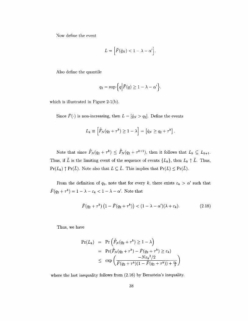
Now define the event

L = [F(N)< < - A -'.

Also define the quantile

q2 = sup {q (q) 1 - A- a'}.

which is illustrated in Figure 2-1(b).

Since F(.) is non-increasing, then L = [4N > q2]. Define the events

Lk [ FN(q2 + Tk) > 1--] [N > q2 + Tk]

Note that since FN(q2 + Tk) < FN(q2 + Tk+l), then it follows that Lk C Lk+1l

Thus, if L is the limiting event of the sequence of events {Lk}, then Lk I L. Thus,

Pr(Lk) I Pr(L). Note also that L C L. This implies that Pr(L) < Pr(L).

From the definition of q2, note that for every k, there exists sk > a' such that

F(q2 Tk) 1 - A - Ek < 1 - A - a'. Note that

F(q2 + Tk1) (q2 + Tk)) < (1 - - )(A + k). (2.18)

Thus, we have

Pr(Lk) = Pr(FN(q2 +rTk ) _l

= Pr(FN(q2 + k) - (q2 + Tk) _> k)

Sexp ( - Ne 2/2F(q2 + Tk)(1 - F(q2 + 7k)) + 1

where the last inequality follows from (2.16) by Bernstein's inequality.

From (2.18), it follows that

Pr(Lk) < exp -Nek2/2-

exp( -Nek/2

Thus, based on similar arguments we can conclude that choosing

N > 4 I1w(1 - w) + )log (

implies that Pr(Lk) < _ for all k. It follows that Pr(L) • Pr(L) < d.

Note that [QN is not a'-accurate] = B U L. Thus, Pr(QN is not a'-accurate) <

Pr(B) + Pr(L) < 6. Thus, for

N N(w, a, 6) = w(1 - w) + - log ,

we have Pr(QN is a'-accurate) > 1 - 6. I

We can now proceed to prove Theorem 2.3.6, which makes use of Bernstein's

inequality.

Proof of Theorem 2.3.6. Suppose a' = '. Then, from Lemma 2.3.8, for

N > --; w(l-w) + log

S (1 - w) + -4 log(2aw a 3 jg1 6

= (9(1 - w) + 4a) log -a2w

it follows that QN is a'-accurate with probability of at least 1 - 6. Since if qN is

a'-accurate, it follows by Corollary 2.3.5 that p(qN) < (1 + a)p(q*). This concludes

the proof of the theorem. I

Since we have previously shown that the regret p(q) of the profit-maximizing

newsvendor and the objective function of the cost-minimizing newsvendor are equiv-

alent we can extend Theorem 2.3.6 to the cost-minimization variant.

Theorem 2.3.9 Suppose Assumption 2.1.1 holds. Consider the cost-minimizing newsven-

dor problem specified by a per-unit holding cost h > 0 and a per-unit backlogging

penalty b > 0. Let 0 < a < 1 be a specified accuracy level and 1-6 (for 0 < 6 < 1) be a

specified confidence level. Suppose that N > N(w, a, 6) - (9(1 - w) + 4a) log( ),where w = min(h) Suppose the SAA counterpart is solved with respect to N i.i.d.

samples of D. Let Q7' be the optimal solution to the SAA counterpart. Then, with

probability of at least 1 - 6, the expected cost of Q• is at most 1 + a times the ex-

pected cost of an optimal solution q* to the newsvendor problem. In other words,

C(Qg) < (1 + a)C(q*) with probability of at least 1 - 6.

We observe that the Hoeffding sample size bound is of the order of magnitude

proportional to 1 log ( ). On the the other hand, the Bernstein sample size bound

is of the order of magnitude proportional to -I log ( ). Therefore, for small values

of w, we expect that the Bernstein sample size bound is significantly smaller than

the Hoeffding bound. Note that if w is small, the optimal order quantity belongs to

extreme quantiles of the demand distribution.

Figures 2-2 and 2-3 illustrate the difference in the bounds provided by Bernstein

and Hoeffding for various levels of w. Notice that if w is close to zero, then there is

a drastic improvement on the sample size required by the Bernstein bound. On the

other hand, if w is close to 1, then the difference between the two bounds is negligible.

Therefore, if w is significantly small, then we can expect a significant improvement

in the order of magnitude of the sample size required by the Bernstein bound. On

the other hand, for the ranges where the Hoeffding bound is better, the improvement

is small.

In the following lemma, we establish conditions on the parameters that would

guarantee that Bernstein's inequality provides a tighter bound on the sample size.

For each accuracy level, the range of w values for which the Bernstein or Hoeffding

Comparison of bounds for maximization variant with w = 0.01 and 8 = 0.01

0 0.2 0.4 0.6 0.8 1

(a) w = 0.01

Comparison of bounds for maximization variant with 0) = 0.05 and 8 = 0.01

0 0.2 0.4 0.6 0.8 1

(b) w = 0.05

Figure 2-2: Comparison of bounds implied by Hoeffding, and Bernstein for the max-imization variant of the newsvendor problem as a function of the accuracy rate, forw = 0.01, 0.05.

103

Comparison of bounds for maximization variant with w = 0.2 and 8 = 0.01

0.2 0.4 0.6 0.8 1

(a) w = 0.2

Comparison of bounds for maximization variant with o = 0.4 and 8 = 0.01j A7

0.2 0.4 0.6 0.8 1

(b) w = 0.4

Figure 2-3: Comparisonimization variant of thew = 0.2, 0.4.

of bounds implied by Hoeffding, and Bernstein for the max-newsvendor problem as a function of the accuracy rate, for

106

0 1010

Q)N(u

E 104

103

0

10U

bound gives tighter bounds are plotted in Figure 2-4.

Lemma 2.3.10 For a specified accuracy level a > 0 and a specified confidence level

1 - 6 (for 0 < 6 < 1), the Bernstein bound in Theorem 2.3.9 is smaller than the

Hoeffding bound in Theorem 2.3.1 if and only if w < L (9 + 4a - 4a(4a + 18)).

Proof. From Theorems 2.3.1 and 2.3.9, it follows that Bernstein's inequality gives a

better bound if and only if

99w 2 - (9 + 4a)w + -> 0. (2.19)

4-

For a fixed a, the left-hand side of (2.19) is a second degree polynomial of w. The

discriminant of (2.19) is given by

A = (9 + 4a)2 - 92 = 4a (4a + 18), (2.20)

which is always nonnegative. Therefore, if we define

Wmin = 9 + 4a - ,18 9+4•- ,

wmax = 9 + 4a + ,

then the bound provided by Hoeffding's inequality in Theorem 2.3.1 is better than

Bernstein in Theorem 2.3.9 only in the range of w E [wmin, Wmax]. Note however that

A > 16a 2. Thus,

Wmax = (9 + 4+x/ V)

1 1> -(8a + 9) > -.

18 -2

Since w = min m, 1 - , we know that w <• . Thus, a necessary and sufficient

condition for the Bernstein bound to be better is for w < Wmin- I

3

0 0.2 0.4 0.6 0.8 1accuracy rate, a

Figure 2-4: Plot of regions of w = min (1 - A, A) for which the Hoeffding or theBernstein bound is tighter, for various accuracy rates, a. The y-axis is in logarithmicscale.

2.4 The Newsvendor Model with Risk Preferences

The assumption of the newsvendor problem discussed in Section 2.1 is that the firm is

risk-neutral. However, under an experimental setting, it has been shown by Schweitzer

and Cachon [37] that ordering choices systematically deviate from those that maxi-

mize expected profit. The firm will often accept a smaller expected profit if it also

yields a smaller risk of returns. Bertsimas and Thiele [5] model this risk-preference by

introducing a single scalar risk parameter that allows the firm to adjust the trade-off

between risk and return. Under a traditional newsvendor model, a risk-neutral firm

chooses an ordering quantity that maximizes its expected profit with respect to all of

the demand scenarios. In contrast, under the model they propose in [5], a risk-averse

firm will choose to protect itself only against a specified set of worst-case scenarios

of the demand. In particular, it will choose an ordering quantity that maximizes the

expected profit conditioning on the demand being less than some specified risk para-

meter. They call this one-sided trimming of the demand. Moreover, Bertsimas and

Thiele [5] propose a data-driven approach based on one-sided trimming to approxi-

mate the optimal order quantity under the newsvendor setting with risk preferences.

In this section, we provide a novel analysis regarding the quality of the solution of

their data-driven approach. The analysis is based on a variant of the SAA approach

under the risk-neutral setting, but with appropriately adjusted parameters.

Suppose 3 is a risk parameter, where / E (0, 1). Let qp be the 1 - /3 quantile of

the random demand D. That is,

qP = inf{qlFD(q) > 1 - 0}.

Without loss of generality, we can assume that FD(qp) = 1 - 3. This is because if

there is a probability mass on qp and FD(qp) > 1 - P, then we can decrease /3 until

this property is satisfied without increasing the risk.

A risk-averse firm will choose a conservative ordering policy that maximizes its

expected profit conditional on the event that D < qp. Define the random variable D =

[DID < qp]. To avoid confusion, all functions and expectations will be subscripted

by the random variable on they are defined. The risk-averse newsvendor problem is

maxg9(q) = pEf[min(, q)] - cqqŽO

= pED[min(D,q)|D < qO] - cq. (2.21)

Note that the objective function is maximized at the A = 1 - E quantile of the random

variable D. In other words, if q* is the solution to the risk-averse newsvendor problem

defined by (2.21), then

q* = inf{q|lF(q) > A}.

Bertsimas and Thiele [5] propose a variant of the SAA approach to solve the

model with risk-preferences. Let N be the total number of observations of the random

demand D. Suppose the samples are ranked in an ascending order and labeled as

d1 < ... < dN. The samples are trimmed by taking the No = [N(1 - 3)] smallest

data. The data-driven counterpart of the newsvendor problem with risk-preferences

is1 No

max p-• min(dk, q) cq. (2.22)qO N k=1

This problem is simply a classical newsvendor problem under the empirical dis-

tribution of b defined by assigning a probability of - for each sample d',..., dN

The solution to the data-driven counterpart is the A quantile of the empirical dis-

tribution. Thus, if we denote qNo to be the optimal solution of the data-driven

counterpart (2.22), then

4NO = inf q 1; E (dk < q) > A}. (2.23)k=1

Since 4No <5 dNo, then qN. is also the rN(l-3)lA sample quantile of the empirical

distribution of D based on all the N samples. That is, 2.23 is equivalent to

Ik [N(1 - )1 (2.24)4N,= inf q N 1(d < q) > N"

k=1

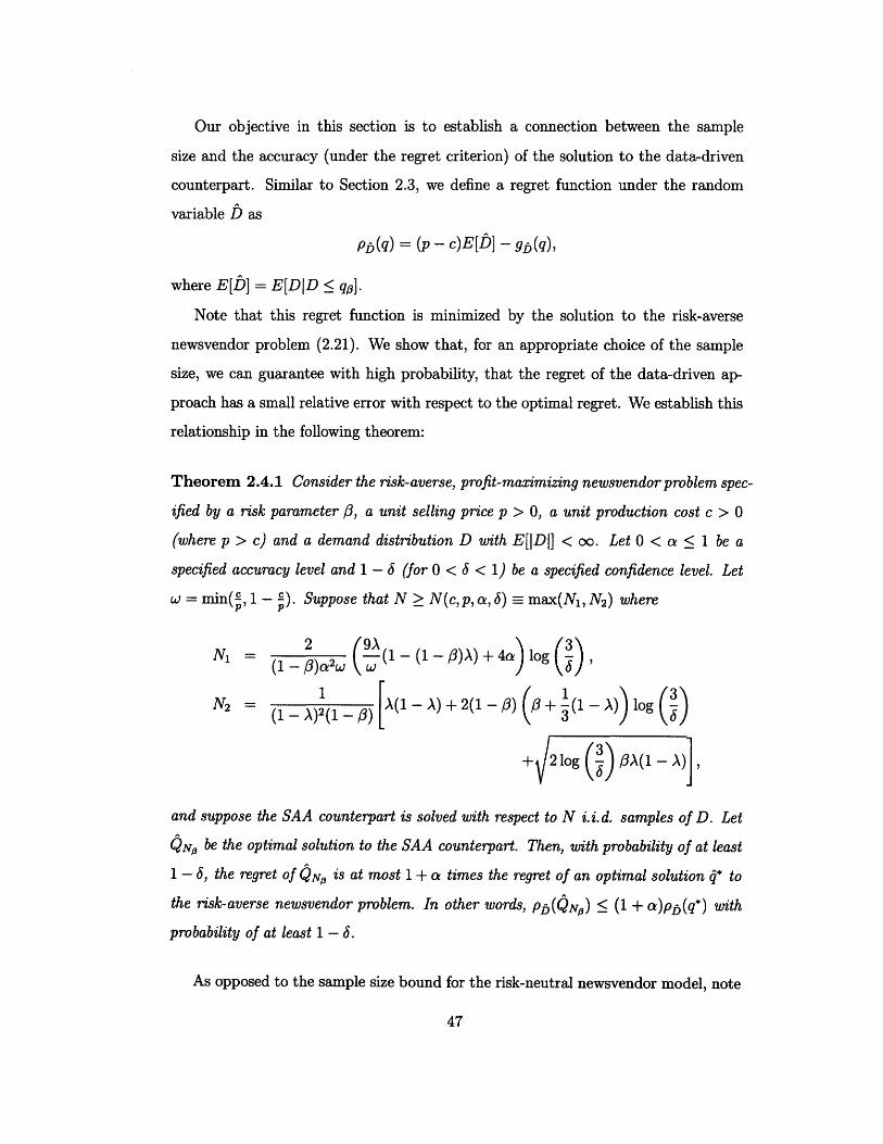
Our objective in this section is to establish a connection between the sample

size and the accuracy (under the regret criterion) of the solution to the data-driven

counterpart. Similar to Section 2.3, we define a regret function under the random

variable D as

PD(q) = (p - c)E[D] - gb(q),

where E[D] = E[DJD < qp].

Note that this regret function is minimized by the solution to the risk-averse

newsvendor problem (2.21). We show that, for an appropriate choice of the sample

size, we can guarantee with high probability, that the regret of the data-driven ap-

proach has a small relative error with respect to the optimal regret. We establish this

relationship in the following theorem:

Theorem 2.4.1 Consider the risk-averse, profit-maximizing newsvendor problem spec-

ified by a risk parameter 0, a unit selling price p > 0, a unit production cost c > 0

(where p > c) and a demand distribution D with E[IDI] < oo. Let 0 < a < 1 be a

specified accuracy level and 1 - 6 (for 0 < 6 < 1) be a specified confidence level. Let

w = min( , 1 - D). Suppose that N > N(c, p, a, 6) - max(N1 , N 2) where

N = ( )a(1 - (1 - 3)A) + 4a log ,

N=(1 - A)2(1 - ) 3

+ 2 log (3) A(1 - A)]

and suppose the SAA counterpart is solved with respect to N i.i.d. samples of D. Let

QNg be the optimal solution to the SAA counterpart. Then, with probability of at least

1 - 6, the regret of QN' is at most 1 + a times the regret of an optimal solution q* to

the risk-averse newsvendor problem. In other words, Pb(QN,) 5 (1 + a)pb(q*) with

probability of at least 1 - 6.

As opposed to the sample size bound for the risk-neutral newsvendor model, note

that the sample size is the maximum of two numbers, N1 and N 2. We will show that

if the sample size is at least N1, then it is guaranteed with probability of at least

1 - 26 that QNo is a'(1 - 3)-accurate with respect to D for a modified newsvendor

problem. On the other hand, N 2 guarantees with probability of at least 1 - ý that

QN is at most the 1 - 0 quantile of D.

If the trimming factor 0 is small, then N 1 inversely proportional to approximately

w, similar to the bound we derived without trimming (risk-neutral firm) in Theo-

rem 2.3.6. We can also see that the bound is inversely proportional to 1 - /. There-

fore, more samples are required if the firm is more risk-averse (i.e., the risk parameter

3 is larger).

We now proceed to prove Theorem 2.4.1. We know from Corollary 2.3.5 that if

4N, is a'-accurate with respect to the distribution of D and A, then the relative error

of its regret Pb(q4N.) is bounded. Therefore, in order to prove Theorem 2.4.1 we need

to establish a relationship between the sample size N and the a'-accuracy of qN. with

respect to D and A.

Note that the random variable D = [DID < qp] has the following cumulative

distribution functions

FD(q_) if q < q0,Fb(q) = 1

1, if q > q0.

{l 1-,FD -

S0, if q > q· .

Thus, if we can ensure that qNO, qp, then the conditions for a'-accuracy of qn4

with respect to D are equivalent to

FD_(No) > (1 - )A - (1 - )a', (2.25)

FD > 1- (1-- ))A - (1-- O)a',

which we can view as conditions for (1 - P)a'-accuracy of 4N, with respect to D

and a modified quantile (1 - O)A. Thus, if we can establish that 4qN. 5 qp and that

conditions (2.25) and (2.26) hold, then it follows that 4N, is a'-accurate with respect

to D. We can then use Corollary 2.3.5 to prove Theorem 2.4.1.

The following two lemmas establish a sample size that guarantees that these con-

ditions hold. We will be using Bernstein's inequality to prove the lemmas since we

have shown in the previous section that it provides an improvement over the sample

size implied by Hoeffding's inequality.

Lemma 2.4.2 For each a' > 0, 0 < 3 < 1 and 0 < 61 < 1, if the number of samples

is N1 > N(',l, 61) (1- (- A(1 - (1 - /3)A) + ) log , then FD(QN.) >

(1 - /)A - (1 - P)a' and FD(QNo) > 1 - (1 - O)A - (1 - 3)a' with probability of at

least 1 - J1, where QN, is the [NA(-7 3)] A sample quantile.

Proof. For ease of notation, let iq(N) = N(1l)]. Note that qr(N) > 1-43 for every N

and 7(N) - 1-/0 as N --+ oo. Define the event B = [FD(qNO) < (1-3)A-- a'(1-/)].

Also define the quantiles of the distribution of D

]1 = inf {q FD(q) > n7(N)A - (N)a',

and

q = inf {q FD(q) 1 -/)A- (1 -3)a'}.

Thus, B = [4N, < qi]. Since 41 2 ql, then B C [4N,, < q1]. Consider a monotoni-

cally decreasing, nonnegative sequence {rk} where Tk 1 0. Define the events

B = N( - rk) > (N)A] < N - Tk],

where FN (.) is the cumulative distribution function of the empirical distribution de-

fined on N samples.

Since FN(Q1 - rk) _< N(q1 - Tk+l), then it follows that Bk C Bk+l. Thus, if B is

the limiting event of the sequence of events {Bk}, then Bk I B. Thus, Pr(Bk) I Pr(B).

Note also that [4N. < 41] _C B. This implies that Pr(B) < Pr(fB).

From the definition of qi, note that for every k, there exists sk > a',q(N) such

that FD(q1 - Tk) i,(N)A - Ek-

FD(41 - k)(1 - FD(1 - Tk)) < (I(N)A - q(N)&) (1 - ,(N)A Ek) .)

We have by Bernstein's inequality

- Pr(PN(4l - Tk) Ž 77(N)A)

= Pr(FPN(41 - Tk) - FD(ql - Tk) > Ek)

-Nek 2/2

From equation (2.26), it follows that

Pr(Bk) exp (((N)A - 7r(N)a') (1 - r(N) E) + 0k)-NEk/2

- TI(N)A) + ,(N)A - n(N)a' +

Since we know that Ek > rq(N)a', then

Pr(Bk) < exp(1(-7(A - o)(I --Nql(N)a'/2

TI(N)A) + l(N)A - 7(N)a' +3

exp ( -Nl)(N)a'/2exp (-A(1- rq(N)A) - + 2,(N)A -+(N)a'}

Also since 1 - 3 _ rq(N) and rq(N)A < 1 - min(rq(N)A, 1 - r(N)A), then, it follows

that

S(1 - P)A) + - 2min(77(N)A, 1 - 77(N)A ) - (N)a'

< exp ( l-N(1 - )a'/2 )-A(1 - (1 - /3)A) 3)

Thus, by choosing

2N> -> )a'

- (1 - 3)a'

a1 A1A(1

log ( 6,

Note that

(2.26)

Pr(Bk)

Tk)(1 - FD(41 - Tk)) + S'

,,,,f'

_- v D((l --

i

4)-(1 - )A) + 3

,.,, /• Y i • 1

-v -L ?I (N)(A-o')( 1

we have Pr(Bk) < . This implies that Pr(B) < Pr(BP) < -.-2 -2

Similarly, define the event L = [FD(q4N) < 1 - (1 - 3)A - a'(1 - P)]. Also define

the quantiles of the distribution of D

2 = SP qFD(q) 1 - 7 N)A - 9 N)a')

and

q2 = sup{ql'D(q) _ 1-(I- )A - (1- ))'}.

Thus, L = [qN, > q2]. Since 42 • q2, then L C [g > q2]. Define the events

Lk N(2 Tk 1 -(N)] = N 2 q +Tk

where FN(') is the probability Pr(D > q) of the empirical distribution defined on N

samples.

Since FN(q 2 + Tk) • FNN(q2 + Tk+1), then it follows that Lk C Lk+l. Thus, if L is

the limiting event of the sequence of events {Lk}, then Lk T L. Thus, Pr(Lk) T Pr(L).

Note also that [4N, > q2] C L. This implies that Pr(L) • Pr(L).

From the definition of q2, note that for every k, there exists Ek > a'r?(N) such

that FD(q2 + Tk) = 1 - (N)A - k

Note that

FD(q2 + Tk)(l - FD(q2 + Tk)) < (1 -D(N)A - 77(N)a') (77(N)A + 6k). (2.27)

We have by Bernstein's inequality

Pr(Lk) = Pr(FN(42 + k) > 1- -(N)A)

- Pr(FN(42 + k) - FD(q2 + k) > Ek)

< exp( -Nek 2/2S D (2 + Tk)(1 - FD( 2 + Tk)) + A

From equation (2.27), it follows that

Pr(Lk) exp - -NE/2(1 - ,q(N)A - 7(N)a') (7(N)A + Ek) + 3

- exp (7(N)A(1 - ?(N)A -NEk/2

-,q(N)o') + 1- -(N)A - 7(N)a'

Since we know that Ek > rl(N)a', then

r(Lk) < exp --N (N)a'/2Pr(Lk) exp 1A(1 (N)A (N)a') -(N - (N)+ (N)A/ - r(N)a'

N'- v -LA (1

Thus, it follows that

Pr(Lk) < exp -N(1 -I)a'/2Pr(L) exp (1 - (1 - ) + - 2+min( r(N)A, 1 - r(N)A) - rI(N)a'

Sexp -N(i - )a'/2Sb-y •,A(1 - (1 -o)A) +

Thus, by choosing

2N 2

-(1O-)a'1A(I - (I - )A) + log ( ,

we have Pr(Lk) < -. This implies that Pr(L) < Pr(L) < 61

Therefore, for N > N(a,,61) (1-)a ('iA(1 - (1 - 3)A) + ) log , we

have the probability of our desired event

Pr(Bc n Lc) = 1 - Pr(B U L) > 1 - Pr(B) - Pr(L) > 1 - 61.

c~Y I

N)a')

Lemma 2.4.3 For each 0 < 62 < 1, if the number of samples is N > N(P, 62), where

N2 = N(ij,62) - A) + 2(1 - 3) /3+ 1(1 - A))3

+ 2log (A(1-A) ]

then N, the N-,) A sample quantile, is at most q6 with probability of at least 1-62.

Proof. Note that for every N, there exists some eN E [0, 1) such that [N(1 - P)] =

N(1-0)+EN. Since qNo is the ) A quantile of the empirical distribution defined

with N samples, then

Pr (qN > qP) Pr ((q) [N(1 - PA)

= Pr (FN(qa) < (1

Also, since FD(qp) > 1 - 3, then

Pr(qN, > qp )

We also know that eN < 1, so it follows that

SPr (FD(q~p) - (qp) > (1 - A)(1 - ) - .

If N > (1-A))- ' then we can apply Bernstein's inequality. For now, let us assume

that this is true. By Bernstein's inequality, we have

Ne E-((1 - A)(1 - _ ) )2Sexp •

log -( 62

1= 1A(1(1 - A)2(1 - 0)

-+ '+ A)

< Pr (FD(qO) - FN(qp) > (1- )(1 -A( - - A.

Pr(qN, > qp)

Pr(q^, > qP)

For Pr(cN. > qP) < 62, we must have

N ((1 - A)(1 - 3) - )N > 2 ((1

Rearranging terms, we get a second degree polynomial in N

(1 - A)2 (1 - )2 N 2 - [2A(1 - A)(1 - 3) + 2(1 - 3) log

2 l()6+A2 + -A log T 20+()3 >0

+ 1(1 - A) N3

where we know if Nmax and Nmin are the roots of the second-degree polynomial

specified by the left-hand side, then the inequality holds if N > Nmax.

The discriminant of the quadratic inequality is

A = 2A(1 - A)(1 - 0) + 2(1 - 3) log -( +L \(612)

-4(1 - A)2 (1 - 3)2

= 4(1 -_3) 2 log

(A

(*) ((13

2 A log3

I13- ))

1(1

3- A)2

log -

which is always nonnegative.

To simplify the terms, note that

(1+= 2(1 - 3) (3+

1-(13

2log )2 +

(1- A) log (8(1 - 0)2 log

+2(1-03) 2log ()1A(1 - A).

Therefore, for

1N >

- (1 - A)2(1 -3)A(1 - A) + 2(1 - 3) ( + (1 - A) log (-)3 ( )2

+ 2 log (•23A(1 - A)

log -(.62(

(1- A)(1 - )- -L- ) + 33

+ 2A(1 - A)O)

S 4(1 -0) 2

2 Nmax,

162)A(1- A)

we have Pr(dNo 5 q,) - 1 - J2. Note that N > , thus it is valid to use

Bernstein's inequality. I

Now we can proceed with the proof of Theorem 2.4.1. In the following proof, we

will be using Lemma 2.4.2 and Lemma 2.4.3.

Proof of Theorem 2.4.1 Define the events S = [qNa > qo], B = [FD(qNo) < (1 -

))A - a'(1 - 0)] and L = [FD(qNO) < 1 - (1 - P3)A - a'(1 - 0)].

Let a'= •. Also let 61 =2• and 62 = . By Lemma 2.4.2, we know that for

N 2 A(1 - (1 -/3)A) + log (N (1- 3)a' 3 J,

6 3 X(1 - (1 - 0)A) + log (3)(1 - O)aw (a 3 6( 1(1 - (1 - O)A) + 4a log (3)(1 - O)a2W ( W 6

then Pr(B U L) _ 61 = . Also, from Lemma 2.4.3, we know that for N > N 1,

we have Pr(S) 5 62 = A. Note that [Sc n B c n Lc] imply that 4N, is a'-accurate

with respect to D. Also from Corollary 2.3.5, we know that if gN, is a'-accurate with

respect to D, then pf(Y4N) < (1 + a)p( *). Thus,

Pr(pb(QN,o) < (1 + a)p(4*)) Ž Pr(QNo is a'-accurate)

> Pr(Sc n B n Lc)

= 1-Pr(SUBUL)

> 1 - Pr(S) - Pr(B U L)

> 1-6-62 =1-6. I

In what follows, we will illustrate the effect of introducing risk-preferences (by

the trimming factor 3) to the sample size required to ensure accuracy of the regret.

We compare the bound in Theorem 2.3.6 for the risk-neutral firm and the bound in

Theorem 2.4.1 for the risk-averse firm. Figure 2-5 compares the two bounds for a

trimming factor f = 0.05 and for critical fractiles A = 0.01, 0.99. Note that even

though there is only a small amount of trimming (0 = 0.05), if A is very large, then

the order of magnitude of the samples for the trimming case is much larger. If A is

small however, the two bounds are comparable.

Figure 2-6 plots the required sample size for the trimmed case as a function of the

trimming factor 0. Notice that as the trimming factor increases, more samples of the

demand are required. This result follows from what we would intuitively expect since

a larger trimming factor means that there are less samples from the random variable

D. This is compensated by taking more samples of the demand D. Also note that

for 3 = 0, the number of samples for the trimmed and the non-trimmed cases are the

same. And as the trimming factor increases, the two bounds diverge.

Comparison of bounds for maximization variant with 0 = 0.05, , = 0.01 and 8 = 0.019 ,

10

(a) A = 0.01

Comparison of bounds for maximization variant with 0 = 0.05, X = 0.99 and 8 = 0.01.,9

0 0.2 0.4 0.6 0.8

(b) A = 0.99

Figure 2-5: Comparison of bounds for the case of trimming and without trimming(trimming factor ,=0.05) as a function of the accuracy level a.

- - without trimmingI- with trimming

SI I I I

- - - without trimming- with trimming

I

109

10"

V-

N

E 106

105

0

Comparison of bounds for maximization variant with X = 0.5 and 8 = 0.01

- with trimming (a = 0.01)- with trimming (a = 0.1)

- - - without trimming (a = 0.01)- - - without trimming (a=0.1)

0.6

Figure 2-6: Plot of the bounds for for the required number of samples in the trimmingcase as a function of the trimming factor p.

· · ·

_ _ _ _ _ _ _ _ _ _ _·_ _ _ _ _ _ _ _ _ _ _·_ _ _ _ _

------------------------- -

0,-1

1 n 4

I

Chapter 3

Numerical Results for the

Data-Driven Newsvendor Problem

with Exogenous Price

In the previous section, we introduced the Sample Average Approximation (SAA)

method as a nonparametric approach for solving the newsvendor problem and its

variants in scenarios where the explicit demand is not known. In this approach it is

assumed that a set of N independent samples of the demand is available. In Chap-

ter 2, we provide a theoretical analysis regarding the number of samples required to

guarantee that the regret of the SAA solution has a bounded relative error compared

to the optimal regret that is computed with respect to the true demand distribution.

However, this bound is only a worst-case bound on the number of samples required.

It is likely that in many cases a significantly smaller number of samples will suffice.

In this chapter, we conduct numerical experiments to evaluate the empirical per-

formance of the SAA approach in different concrete scenarios. In particular:

* We explore how the SAA approach performs as the critical newsvendor fractile

A varies under various concrete demand distributions.

* We explore the sensitivity of the approach to different parameters of concrete

distributions.

* We compare the performance of the SAA approach to other approaches for

solving the newsvendor problem with partial demand information.

* Compare the theoretical and empirical confidence levels to achieve a specified

accuracy of the regret of the SAA approach.

In particular, we consider the minimax regret approach and a parameter-estimation

approach. The minimax regret approach minimizes the opportunity cost of not mak-

ing the optimal decision over a family of distributions to which the true demand

distribution is assumed to belong.

In addition, we compare the SAA approach to the classical parametric approach.

In this approach, the demand is assumed to belong to a certain parametric family of

distributions, and the data is used to estimate the corresponding parameters. After

that, the analytical model is solved with respect to the estimated parameters.

The remainder of the chapter is structured as follows. Section 3.1 outlines ex-

periment design as well as the performance measures of the numerical experiments.

In Section 3.2, we present the results of the numerical experiments. We also make

observations and present our insights from these results.

3.1 Methodology

We outline the steps of the SAA approach as we apply it in our numerical experiments.

* A set of N samples d',..., dN, is drawn from the true demand distribution.

* We denote 4N as the A = -- sample quantile.

* The first two steps are repeated independently for a total of m times.

The optimal solution to the SAA counterpart with N samples, QN, is a random

variable that is dependent on the specific N samples of the demand D. The procedure

outlined above is repeated for a total of m times to approximate a distribution for

QN and the absolute error of the SAA quantity IQN - q* , the expected profit g(QN)

and the regret p(QN), where q* is the optimal order quantity under full knowledge of

the demand.

In the experiments, we take N = 100 samples for m = 100 runs of the procedure.

We generate data from five distributions: uniform, normal, exponential, Pareto and

Poisson. In the base case, the unit price is set to p = 3 and the cost is c = 1 The

specifications of the distribution in the base case are as follows:

Uniform range of [0, 2p] with p = 50

Normal mean p = 50 and standard deviation a = 25

Exponential mean p = 50

Pareto mean p = 50 and range [1, oo)

Poisson mean p = 50

In analyzing the sensitivity to the critical fractile, the price is p = 3 and the unit

cost takes on values c E 3 x [0.05,0.10,..., 0.95].

The sensitivity analysis of the SAA procedure to various distribution parameters

is conducted with the following specifications

Uniform I E [12.5, 25,... , 250]

Normal p E [12.5, 25,..., 250]

a [2.5, 5, ... , 50]Exponential p E [10, 20, ... , 200]

Pareto k E [1, 2,...,50]

In the minimax regret approach, a family of distributions with mean # = 50 is

assumed. The distributions used to compare with the minimax regret order quantity

are: uniform, normal, exponential and Poisson, with parameters specified in the base

case above.

In the parameter-estimation approach, data is generated from the following distri-

butions: uniform, Pareto, exponential and Poisson, where the parameters are specified

by the base case above. The data is then fitted to different distributions to estimate

the parameters.

In comparing the theoretical and empirical confidence levels achieved by the

regret of the SAA approach for specified accuracies, we consider accuracy rates

a E [0.05,0.10, ... , 0.95] and critical fractiles A = 0.1,0.5,0.9. We take N = 100

and repeat the SAA procedure for m = 100 runs. The theoretical confidence levels

are computed from the Bernstein and Hoeffding bounds (Theorem 2.3.1 and Theo-

rem 2.3.9). If the theoretical confidence level computed is negative, we simply set it

to zero. Suppose q^ is the SAA ordering quantity for k = 1,..., m. The empirical

confidence level is computed by the following formula

1 mEmpirical Confidence Level = M 1(p(k) < (1 + a)p(q*))

mk=l

where 1(-) is the respective indicator function and q* is the optimal ordering quantity

under full knowledge of the distribution.

The performance of the SAA approach is evaluated by observing the relative error

of the average expected profit and average regret. In particular, if qk is the SAA

ordering quantity for the kth run for k = 1,..., m, then

m

Average Absolute Error of the Order Quantity = 1 k - q *

k=1

g(q*) - g(q•)Average Relative Error of the Expected Profit -= ) = 1

g(q*)1 ZM1 p(q - p(q*)

Average Relative Error of the Regret = m(k=p(q*)

where q* is the optimal order quantity under full knowledge of the distribution.

3.2 Results and Discussion

We present the results of our numerical experiments in this section as specified by

the experimental design in Section 3.1.

a Theoretical Confidence Level Empirical Confidence LevelHoeffding Bernstein Uniform Normal Exponential Pareto

0.05 0 0 0.971 0.99 0.998 10.1 0 0 0.999 0.999 1 10.15 0 0 1 1 1 10.2 0 0 1 1 1 10.25 0 0 1 1 1 10.3 0 0 1 1 1 10.35 0 0 1 1 1 10.4 0.17778 0.12779 1 1 1 10.45 0.3507 0.29597 1 1 1 10.5 0.5013 0.44506 1 1 1 10.55 0.62746 0.57285 1 1 1 10.6 0.72933 0.67894 1 1 1 10.65 0.80873 0.76438 1 1 1 10.7 0.86854 0.83121 1 1 1 10.75 0.91213 0.882 1 1 1 10.8 0.94287 0.91952 1 1 1 10.85 0.96387 0.94647 1 1 1 10.9 0.97778 0.9653 1 1 1 10.95 0.98671 0.97808 1 1 1 1

Table 3.1: Theoretical and empirical confidence levels for various accuracy levels ofthe solution to the SAA counterpart of the profit-maximizing newsvendor with criticalfractile A = 0.5

Influence of the Critical Fractile

Figure A-1 plots the average of the error IqN - q*j as a function of the critical fractile.

Figure A-2 plots the relative error of the expected profit and the regret achieved by

the SAA counterpart as a function of the critical fractile.

Tables 3.1-3.2 summarize the theoretical and empirical confidence levels achieved

by various distributions for A = 0.1, 0.5, 0.9.

We make the following observations:

* In most of the demand distributions considered, the error IqN - q*l generally

increases as the critical fractile increases. This is especially true of demand

distributions that are unbounded from above (see Figure A-1).

* The relative error of the expected profit of the SAA solution is highly sensitive

to the critical fractile (see Figure A-2(a)). In particular, the error is larger for

a Theoretical Confidence Level Empirical Confidence LevelHoeffding Bernstein Uniform Normal Exponential Pareto

0.05 0 0 0.946 0.924 0.906 10.1 0 0 0.995 0.991 0.976 10.15 0 0 0.997 1 0.995 10.2 0 0 0.999 1 0.999 10.25 0 0 1 1 1 10.3 0 0 1 1 1 10.35 0 0 1 1 1 10.4 0 0 1 1 1 10.45 0 0 1 1 1 10.5 0 0 1 1 1 1

0.55 0 0 1 1 1 10.6 0 0 1 1 1 1

0.65 0 0 1 1 1 10.7 0 0 1 1 1 1

0.75 0 0 1 1 1 10.8 0 0 1 1 1 1

0.85 0 0 1 1 1 10.9 0 0 1 1 1 1

0.95 0 0 1 1 1 1

Table 3.2: Theoretical and empirical confidence levels for various accuracy levels ofthe solution to the SAA counterpart of the profit-maximizing newsvendor with criticalfractile A = 0.9

smaller values of A, which is partly influenced by the small optimal profit at

small critical fractiles. In contrast, the relative error of the regret of the SAA

solution is generally invariant of changes in the critical fractile (see Figure A-

2(b)).

* The Pareto distribution achieves the lowest relative error in the regret (see

Figure A-2(b)) for all critical fractiles, despite having infinite variance (k < 2).

* In the range of critical fractiles, the largest relative error of the expected profit

is of the order 100. The largest relative error of the regret is of the order 10-1.

* From Tables 3.1-3.2, we observe that the theoretical confidence level are much

smaller than the empirical confidence levels for N = 100. In particular, the

empirical confidence levels are very high even with a small accuracy level. This

verifies that the bounds we derive in Chapter 2 are worst-case bounds (i.e., the

sample size required for the regret to achieve a certain accuracy and confidence

level is much smaller than what we derive).

Influence of the Distribution Parameters

Figure A-3 plots the average relative error of the expected profit and the regret

achieved by the SAA counterpart as a function of the mean of a uniform distribution.

The errors are compared for critical fractiles A = 0.1, 0.5, 0.9.


achieved by the SAA counterpart as a function of the mean of a normal distribution.

The errors are compared for critical fractiles A = 0.1, 0.5, 0.9.


achieved by the SAA counterpart as a function of the standard deviation of a normal

distribution. The errors are compared for critical fractiles A = 0.1, 0.5, 0.9.


achieved by the SAA counterpart as a function of the mean of an exponential distri-

bution. The errors are compared for critical fractiles A = 0.1, 0.5, 0.9.


achieved by the SAA counterpart as a function of the parameter k of a Pareto distri-

bution. The errors are compared for critical fractiles A = 0.1, 0.5, 0.9.


The relative error of the regret of the SAA solution is invariant of the demand

distribution parameters (see Figures A-3(b), A-4(b), A-5(b), A-7(b)). In con-

trast, the relative error of the expected profit of the SAA solution is highly

sensitive to changes in the distribution parameters (see Figures A-3(a), A-4(a),

A-5(a), A-7(a)).

Comparison to other approaches

Figures A-8-A-9 compare the relative error of the regret of the minimax regret order

quantity and SAA order quantity to the true optimal order quantity as a function of

the critical fractile, A.

Figures A-10-A-11 compare the relative error of the regret of the parameter-

estimation order quantity and SAA order quantity to the true optimal order quantity

as a function of the critical fractile, A.


* Generally, the SAA method achieves a lower relative error in the regret than the

minimax regret approach (see Figures A-9 and A-8). The only exception is for

the exponential distribution (A-9(a)) which achieves an accuracy comparable

and sometimes even better than that of the SAA method. This is because

the exponential distribution is expected to be the most robust, given that it

is entropy-maximizing over the class of nonnegative distributions with known

mean (Perakis and Roels [28]).

* If the assumed distribution differs greatly from the true demand distribution,

then the parameter estimation approach achieves very high relative errors (e.g.,

data from a uniform distribution fitted to a Pareto distribution in Figure A-

10(a)). On the other hand, if the assumed distribution has similar properties

to the true demand distribution, then the parameter estimation approach can

achieve low relative errors comparable to that of the SAA approach (e.g., data

from a uniform distribution fitted to a normal distribution in Figure A-10(a)

where the normal distribution preserves symmetry of the uniform distribution).

* From the numerical experiments, the regret of the solution to a parameter-

estimation approach can grow up to 1015 times the optimal regret of the true

distribution (see Figure A-10(a)).

* From the numerical experiments, the regret of the solution to the minimax regret

approach can grow up to 100 times the optimal regret of the true distribution

(see Figure A-8(a)).

From the numerical experiments, we can conclude that under the regret criterion

(i.e., small relative error of the regret) the SAA approach provides a consistently good

estimate of the optimal order quantity that is invariant of external demand factors

(e.g. mean or variance). Moreover, it generally performs well against other ap-

proaches, namely the minimax regret approach and parameter-estimation approach.

Chapter 4

Data-Driven Approach to the

Price-Setting Newsvendor Problem

In this chapter, we consider the price-setting newsvendor problem under the assump-

tion that the explicit demand distribution is not known. We assume that the demand

is composed of a deterministic component and a random component. The deter-

ministic demand is a linear function of the price. In contrast to the nonparametric

data-driven approach described in in Chapter 2, we assume that the parameters of

the deterministic demand are known. On the other hand, we assume that the only in-

formation known about the random component is a set of independent samples drawn

from the true distribution. We describe and analyze a simulation-based approach pro-

posed by Zhan and Shen [42] for solving the price-setting newsvendor problem under

partial information on the demand. Specifically, we provide a theoretical analysis of

the number of samples required to achieve a good quality solution with high proba-

bility.

The price-setting newsvendor problem is an extension of the classical newsvendor

problem that incorporates price as a decision variable. Consider a firm selling a

product over a single sales period. The firm must produce units of the commodity

at the beginning of the period prior to observing the demand for the product. The

firm must also simultaneously set the unit selling price. The firm faces a stochastic

demand for that product, which depends on the selling price. The actual demand

occurs during the sales period and is satisfied as much as possible with the units

produced. The firm incurs a cost proportional to the production quantity. Any

unmet demand is assumed to be lost. The objective of the firm is to then maximize

its expected profit.

Studying the price-setting newsvendor problem can provide excellent insights on

how operational problems (i.e., production decisions) interact with marketing issues

(i.e., pricing decisions) to influence decision-making for a firm. Moreover, even though

the integration of pricing and production decisions is in early stages in most man-

ufacturing companies, it still has the potential to radically improve supply chain

efficiencies [11]. Thus, the coordination between pricing and production decisions is a

relevant research direction in revenue management with many practical applications.

Whitin [40] was the first to incorporate pricing decisions in the newsvendor prob-

lem. He showed how to optimize the price and order quantity decisions under the

assumption that the deterministic demand is a linear function of the price. Mills [26]

and Karlin and Carr [21] study the effect of the particular form of demand uncer-

tainty to the pricing decision. Mills [261 showed that for an additive demand model,

the optimal price under uncertain demand is at most equal to the optimal price under

the assumption of deterministic demand (or the optimal riskless price). The optimal

riskless price is the price that maximizes the expected profit under the assumption

that the demand is known beforehand. Conversely, Karlin and Carr [21] find that

the optimal price is at least the riskless optimal price for the multiplicative model of

uncertain demand. A unified framework to reconcile this apparent contradiction has

been provided by Petruzzi and Dada [30].

There have been numerous extensions to the price-setting newsvendor problem in

the recent years. For instance, Dana and Petruzzi [12] consider a model where the

demand depends on both the price and inventory levels. Raz and Porteus [32] remove

the distributional assumption about the random demand component (e.g. additive

or multiplicative) by assuming demand is a discrete random variable that depends

on price. Bernstein and Federgruen [3] study a model with many newsvendors. For

an extensive overview of recent developments in the area of price and production, we

refer the reader to [11].

A common assumption in most inventory models with stochastic demand is that

the underlying demand distribution is known exactly. Although this results in tractable

models, it does not hold in many realistic settings where the demand distribution is

often unknown. Instead of full knowledge of the demand, usually there is only imper-

fect information (e.g. moments of the distributions or historical price-demand data).

Researchers have looked at different approaches to solve the price-setting newsvendor

problem under the assumption of imperfect information.

A popular approach to address imperfect information for an inventory model with

simultaneous pricing and inventory decisions is through a "demand learning" ap-

proach. Monahan, Petruzzi and Zhao [27] apply a dynamic pricing to the newsvendor

model and establish a practical and efficient algorithm for computing optimal prices.

Another approach proposed by Raz and Porteus [33] is by approximating the

demand distribution with a finite number of fractiles and assuming that the fractile

functions are piecewise linear functions of the price. They propose an algorithm that

finds the optimal price-quantity pair by a method of elimination. The advantage of

this approach is that it applies to more general cases of the demand than the case

of additive of multiplicative uncertainty. On the other hand, the method requires

enough demand samples for each price level to accurately approximate the demand

fractiles.

An alternative method proposed by Zhan and Shen [42] uses the Sample Average

Approximation (SAA) scheme to approximate a system of two equations that are

derived from the first-order conditions of the problem. They propose a gradient

search algorithm to solve the data-driven approximation of the first-order conditions.

Although they assume a linear price-demand relationship with known parameters, but

with no additional assumptions on the distribution of the stochastic term. However,

Zhan and Shen [42] do not provide a theoretical framework for the algorithm. In

particular, it is of interest to know how the accuracy of the simulation-based approach

relates to the number of samples of the data.

In this chapter, we extend the results of Zhan and Shen [42] by providing a theo-

retical framework for the simulation-based approach as a method to solve the price-

setting newsvendor problem. Our goal is to establish a relationship between the

sample size and the accuracy of the simulation-based approach as an approximation

to the price-setting newsvendor problem. We derive a bound on the sample size that

ensures with high probability that the regret of the solution to the simulation-based

approach has a small relative error with respect to the regret of the optimal policy un-

der full knowledge of the demand distribution. This bound is applicable for demand

distributions with a random component having bounded support.

The remainder of the chapter is structured as follows. Section 4.1 introduces

the price-setting newsvendor problem where the characterization of the uncertainty

is fully known. We will show that under certain assumptions on the model, the

optimal policy uniquely solves certain first order conditions. Section 4.2 introduces

the simulation-based approach proposed by Zhan and Shen [42]. Finally, Section 4.3

establishes the connection between the sample size and the accuracy of the simulation-

based approach as an approximation to the price-setting newsvendor problem.

4.1 The Price-Setting Newsvendor Model

In this section, we consider the price-setting newsvendor model. The problem deals

with determining a simultaneous pricing and ordering decision for a firm to max-

imize profit under uncertain demand. The demand distribution is assumed to be

known. Petruzzi and Dada [30] provide a review and extensions of the price-setting

newsvendor problem.


First let us define the following notation, which we will be using throughout the

chapter:

c unit cost

p unit selling price

q order quantity

D(p, E) random demand

y(p) deterministic demand

f random component of the demand

F(.), f(-) cumulative and probability density distribution of E

A random demand D(p, E), which is a function of the price, occurs for a single

commodity in a single period. At the beginning of the period, the firm decides how

many units of the commodity to order to satisfy the random demand. The q units

are ordered at a cost of c. The firm simultaneously decides on a unit selling price

p for the product. During the period, the actual demand D(p, e) (the realization of

D(p, E), whose distribution is affected by p) is observed. The firm sells the minimum

between the demand and the number of units ordered at the selling price p. The

profit of the firm is given by

r(q, p) = p min(D(p, e),q) - c q.

Since the actual demand is not known when pricing and ordering decisions are

made, a sensible objective for the firm is to maximize the expected profit. Thus, the

problem is equivalent to

max g(p, q) = E[7r(q, p)] = p E[min(D(p, e), q)] - cq. (4.1)p, q

A feasible pricing and ordering policy is one for which the price and the order

quantity are nonnegative. However, we do not need to impose constraints on the

problem because, as we will see in Proposition 4.1.2, the optimal solution is always

feasible.

We will assume that the deterministic demand is a linear function of the price.

We have

y(p) = a - bp (4.2)

where a and b are known positive constants. Consistent with Mills [26], we assume

an additive form of the demand uncertainty. The random demand function is given

by

D(p, E) = y(p) + 1 (4.3)

where E is the random component of the demand that can assume values in [A, B]. We

assume that E is a continuous random variable consistent with the models of Petruzzi

and Dada [30]. A standard assumption of the additive model is that A + a > 0.

This guarantees that the demand is positive for some valid range of the selling price.

From a practical standpoint, however, it is enough to assume that a+±1 is significantly

greater than a. This allows us to include unbounded distributions, such as the normal

distribution in modeling the demand.

4.1.2 Optimality Conditions

We follow the analysis of Zhan and Shen [42] to derive optimality conditions for the

price-setting newsvendor problem.

We can find a convenient expression of the problem consistent with Ernst [14] and

Thowsen [39] by defining z = q - y(p), which corresponds to the quantity ordered

above the deterministic demand. If the choice of z is above the realized value of e,

then leftovers occur; if the choice of z is smaller than the realized value of E, then

shortages occur. The problem is then reduced to

max g(z,p) (4.4)p, z

where

g(z, p) = E[r(z, p)] = (p - c)y(p) + p E[min(E, z)] - cz.

Therefore, the price-setting newsvendor problem is equivalent to solving the problem

defined by (4.4). For simplicity in our analysis, we will be making the following

assumptions:

Assumption 4.1.1 The random demand component E has bounded support.

Assumption 4.1.2 The optimal riskless price pO = a+b is strictly greater than2b

B-A2b

Assumption 4.1.3 The hazard rate r(z) = f satisfies r2(z) + > 0 for1F (z) +odzz E [A, B].

Note that the optimal riskless price

a + bc + p2b

in Assumption 4.1.2 represents the optimal price under the assumption of determinis-

tic demand. If the firm knows beforehand that the demand as a function of the price

is y(p) + e (where e is a realization of the random component e of the demand), then

it will order exactly y(p) + e units. To maximize the expected profit, it will set a price

p0 that maximizes the expected profit under the riskless scenario (p - c)(y(p) + p,).

Note that Assumption 4.1.3 is satisfied by all nondecreasing hazard rate distrib-

utions, which include uniform, normal, logistic, chi-squared and exponential distrib-

utions (see [42]).

In the literature (see for example Whitin [40]; Zabel [41]), researchers usually

reduce the original problem to an optimization problem over a single variable z.

Zhan and Shen [42] on the other hand describe an approach by working directly on

the first order conditions of the problem. We will be following the approach of Zhan

and Shen [42] to find the optimality conditions to the problem.

The first-order conditions of the price-setting newsvendor problem are

8g = -c + p(l - F(z)) = 0, (4.5)Og

= a + bc - 2bp + E[min(z, e)] = 0, (4.6)

where F(.) is the cumulative distribution function of e.

Note that, if (4.5) and (4.6) form a system of equations, then this implies the

following relationship between z and p:

z(p) = F - 1 - ), (4.7)

p(z) = po - (u- z)f (u)du, (4.8)

where po is the riskless optimal price.

Note that p(z) is a concave function of z. Under Assumption 4.1.3, z(p) is a

concave function of p. Zhan and Shen [42] show that under this assumption, both

curves intersect in at most two points. Note that any solution to this system satisfies

the first order conditions. They have the following proposition:

Proposition. 4.1.1 [Zhan and Shen [42]]. Suppose F(-) is a distribution function

satisfying Assumption 4.1.3.

(1) If a - bc + A > 0, then equations (4.7) and (4.8) have a unique solution, which

is also optimal for the problem.

(2) If a - bc + A < 0 and f(A) < , then equations (4.7) and (4.8) have

two solutions. The one with the larger p value is the optimal solution for the

problem.

(3) If a - bc + A < 0 and f(A) > a+bc+A, then equations (4.7) and (4.8) have no

solution.

Note that Assumption 4.1.2 implies that a - bc + A > B - p. Therefore, Assump-

tions 4.1.2-4.1.3 imply that Case (1) of Proposition 4.1.1 holds. In other words, the

first order conditions have a unique solution which is also optimal to the problem.

Thus, if we define (z*,p*) as the solution to the price-setting newsvendor problem,

then the following relationship holds under Assumption 4.1.2:

z* F- 1 - (4.9)

p· = (a + bc + E[min(z*, E)]). (4.10)2b

For simplicity of notation, we define the following quantities

B-APmin b= po (4.11)2b

Pma = b (4.12)2b

The following Proposition establishes bounds on the solution to the first-order

conditions.

Proposition. 4.1.2 Under Assumption 4.1.1, if (z*,p*) satisfies the first-order con-

ditions (4.5) and (4.6), then (1) A < z* < B, (2) c < p* < pO, (3) p* > pmin, and

(4) q* = z* + y(p*) > 0, where Pmin = pO - (B - A).

Proof. Note that (1) clearly follows from condition z* = F- •).

To prove (2), note that the lower bound follows since the first order conditions

imply F(z*) = 1- p, which only makes sense when p* > c. Also, equation (4.10) im-

plies that p* = pO - (u- z)f(u)du. Since B(u- z)f(u)du is always nonnegative,

then this implies that p* < p0

To prove (3), note that the first order conditions imply p* = pO _ (u

z*)f(u)du. Note that f L(u - z*)f(u)du > (B - z*) Pr(E > z*) _ (B - z*). Also from

(1), we know that z* > A. Thus, p* > pO - (B - A).

To prove (4), note that, from equation (4.10), we know that z* > E[min(z*, E)] =

2bp* - a - bc. Therefore, q* = z* + a - bp* > b(p* - c) > 0, where the last inequality

follows from (2). 1

From (4) of Proposition 4.1.2, note that the solution to the first order conditions

(z*, p*) always provide a feasible (i.e., nonnegative) ordering quantity q*.

4.2 Simulation-Based Procedure

One common approach to approximate the expected value of a random function is

the Sample Average Approximation (SAA) method. In this method, the function is

approximated by taking the average value over finitely many independent samples

that are drawn from a probability distribution.

In the previous section, we have shown that under Assumptions 4.1.2-4.1.3, the

optimal solution uniquely solves the first-order conditions (4.5)-(4.6). If an explicit

cumulative density function of the demand is known, then a gradient search algorithm

can be used to find the optimal pricing and ordering policy. However, in most realistic

settings, the firm may not know the exact distribution that the demand follows.

Usually, the only information available to the firm is historical price-demand data

from past periods. If we know that the deterministic demand is a linear function of

the price, these data imply realizations of the random component E. Therefore, we

can approximate the first-order conditions by the SAA method with a function that

depends on realizations of the random component e. This simulation-based approach

for solving the optimal pricing and ordering policy of the price-setting newsvendor

problem has been proposed by Zhan and Shen in [42].


Suppose that the only information available to a firm is a set of N price-demand

pairs {(dk ,pk)N=l1. We assume that the deterministic component of the demand is

a linear function of price with known parameters. Suppose the demand uncertainty

is additive. Therefore, we can find the corresponding realizations of the random

component using the transformation Ek = dk - (a - bpk) for k = 1,..., N. This data

allows us to obtain the data-driven approximation of the first-order conditions:

-c + p 1 - N(z)) =0, (4.13)

a + bc - 2bp + EN [min(z, E)] = 0, (4.14)

where

N

FN(Z) = 1(Ek < z), (4.15)k=1N

FN(z) = 1(Ek z), (4.16)k=1N

EN[min(z, E)] = NZ min(z, ck). (4.17)k=1

Let (ZN, PN) denote the solution to the data-driven approximation of the first-

order conditions with N samples. Note that (ZN, PN) are random variables that

depend on the specific N samples of E. Let (zN, fN) be the realization of (ZN, N)

for a specific N samples of E.

Proposition. 4.2.1 If (ZN, 1N) is the solution to the data-driven approximation to

the first-order conditions, then (1) A< ZN • B, (2) c < P pN PON 5 Pax, and (3)

PN o - (B -_A), where j3o = a+b+ and AN = 1 EN =k

Proof. The proof of (1), (2) and (3) is similar to the proof in Proposition 4.1.2 since

FN () is the cumulative distribution function of the empirical distribution defined by

the N samples.

4.3 Relative Error of the Regret of the Solution to

the Simulation-Based Procedure

In Section 4.2, we have introduced the simulation-based method proposed by Zhan

and Shen [42] for solving the price-setting newsvendor problem. A natural question

to ask is how many samples are required in order to ensure with high probability

that the simulation-based procedure provides a "good" solution to the price-setting

newsvendor problem.

It is natural to think of an approximation to the price-setting newsvendor problem

being "good" if the relative error of its expected profit is small. A potential com-

plication with this criterion is that the expected profit is not guaranteed to be well

above zero. To circumvent this problem, we instead consider a minimization problem

having the same solution as the price-setting newsvendor problem. If we can show

that the approximation evaluated at this new objective function has a small relative

error, then we can say that it is a "good" approximation of the optimal solution of

the price-setting newsvendor problem.

As mentioned previously, under a scenario where the firm knows the demand

beforehand, pO = is the price it will set to maximize the expected profit under

this scenario. In particular, the expected profit the firm will receive is (po - c)(a -

bpo + pI). Under demand uncertainty, the firm cannot achieve a profit greater than

this. Since we also know that c < po < Pmax = , then a valid upper bound for

the expected profit under demand uncertainty is (Pmax - c)(a - bc + Mi). Therefore,

we can define the regret function

p(z, p) = (pmax - c)(a - bc + iM) - g(z, p), (4.18)

where p,,ax = 2a+b+B

The price-setting newsvendor problem is equivalent to the problem of minimiz-

ing p(z,p). Therefore, the optimal policy (z*,p*) also minimizes the regret func-

tion p(z, p). In this chapter, we will say that an approximation to the price-setting

newsvendor optimal policy is accurate if the relative error of its regret is small. Con-

sider any specified accuracy level a > 0 and confidence level 1 - 6. We will show that

there exists a number of samples N that depend on the the accuracy and confidence

level as well as the parameters of the model, such that with probability of at least

1 - 6, the solution to the simulation-based approach defined on N samples has a

regret p(2N, PN) of at most (1 + a)p(z*, p*).

Since (2 N, PIN) is the solution to the data-driven approximation of the first-order

conditions, it is useful to define a property that (ZN,PN) approximately solves the

first-order conditions. We state the following definition.

Definition 4.3.1 Let (ZN,PN) be some realization of (ZN, PN). We say that (.N,7PN)

is (a',a)-accurate if -a' < 1- F(iN) --- 2 c• and -a' < a+bc+E[min(£N, E)] -

2bPN < a', for some a', a' > 0

The implication of ( N, PN) satisfying the conditions for (a', a')-accuracy is that

for sufficiently small a' and a', the approximation (ZN, PN) "almost" satisfies the

first-order conditions (4.5) and (4.6).

4.3.1 Accuracy of the Regret of a First-Order Approximate

Policy

We would like to show that (a', a')-accuracy of the data-driven solution relates in

some way to the optimal policy of under full knowledge of the distribution. In partic-

ular, we would like to show that the regret of the data-driven policy p(^ N, N) has a

bounded relative error with respect to p(z*, p*). We will show this in a two-step analy-

sis. In what follows, we show that if (^N, 3N) is (a', a')-accurate and I|-ILl < 2bry for

some -y > 0, then the data-driven policy under a modified one-dimensional problem

(with either price of quantity fixed) has bounded relative error. Specifically:

(1) There exists 31 > 0 such that (1--Pl)p(z*, ^) 5 p(z*,p*) [refer to Lemma 4.3.4];

(2) There exists 32 > 0 such that (1--3 2)p(iN, 3PN) < p(Z*,~N) [refer to Lemma 4.3.7];

The combination of these one-dimensional problems implies that the regret of the

two-dimensional problem has a bounded relative error. In what follows, we prove the

relationship between (a', a')-accuracy and the relative error of the regret. We do this

by the two-step analysis we outline above.

First, we establish the following result:

Lemma 4.3.1 Suppose Assumption 4.1.1 holds. Let (iN,PN) be a (a',a')-accurate

realization of (ZN,PN), and (z*,p*) be the solution to the first-order conditions (4.5)

and (4.6). Then IE[min(z*, E)] - E[min(iN, E)]1 5 (1 + a')(B - A).

Proof. Consider the case where z* < •N- If e < z*, then min(z*, E) - min(•N, E) =

0. On the other hand, if E > z*, then min(z*, e) - min(iN, ) > z* - ZN. Thus,

E[min(z*, )] - E[min(ýg, E)] Ž (z* - ^g)(1 - F(z*)) = Iz* - Since we know

that Iz * - ^ I < B - A and p* > c, then it follows that E[min(z*, e)] - E[min(^N, E)] 2

-(B - A) > -(1+ a B)(B - A).

Now consider the case where z* > gN. If e < ZN, then min(z*, e) - min(Ng, e) = 0.

On the other hand, if e > gN, then min(z*,c) - min(gN, ) • z* - iN. Thus,

E[min(z*, e)] - E[min(•g, e)] 5 (z* - ýN)(1 - F(^N)). Since we know that Iz* -

ZNI _ B - A and (•N,1gN) is (a', a')-accurate, then it follows that E[min(z*, e)] -

E[min(N, e)] + al) (B - A). Also, since PgN > c, then E[min(z*, c) -

E[min(Ng, e)] _ (1 + a')(B - A).

Thus combining the two cases, we have proved the desired result.

First Step of Two-Step Analysis

In the next three lemmas, we accomplish the first part of the proof of Theorem 4.3.8.

This is accomplished in the following steps:

(1) We first establish an upper bound for g(z*,p*) - g(z*,pN) [Lemma 4.3.2].

(2) Next, we establish a lower bound for p(z*,gN) [Lemma 4.3.6].

(3) By appropriately choosing 01, we have (1-l 3 1)p(z*, gN) • p(z*, p*) [Lemma 4.3.4].

Lemma 4.3.2 Suppose Assumption 4.1.1 holds. Let (^N, PN) be a (a', a') -accurate

realization of (ZN, iN), and (z*, p*) be the solution to the first-order conditions (4.5)

and (4.6). Then g(z*,p*) - g(z*, ^) (a'2 + (1 + c)(B - A)) Ip* - ^NI.

Proof. From the expected profit formula, we know that

g(z*,p*) - g(z*, I) = (a + bc + E[min(z*, i)])(p* - /N) - b(p*)2 + b(pN) 2 .

Consider the case when p* <I N. Then, from Lemma 4.3.1 it follows that

g(z*,p*) - g(z*,7N) < (a + bc+ E[min(N, e)]

-(1 + ac)(B - A)) (p* - PN) - b(p*)2 + b(PN)2.

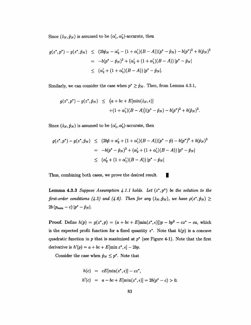
Since (zN, PN) is assumed to be (a', a')-accurate, then

g(z*,p*) - g(z*,Py) (2bP - a' - (1 + a)(B - A))(p* -1g) - b(p*) 2 + b(pyN) 2

= -b(p* - N)2 + (oa' + /d+ a/) (B - A)) jp* - PNI

S(a/ + (1 + a')(B - A)) Ip* - aN.

Similarly, we can consider the case when p* 2 ^N. Then, from Lemma 4.3.1,

g(z*,p*) - g(z*, PN) • (a + bc + E[min(iN, e)]

+(1 + a')(B - A)) (p* - PN) - b(p*)2 + b(3gN) 2.

Since (SN, PN) is assumed to be (a', c')-accurate, then

g(z*,p*) - g(z*,Pg) • (2b + a +(1 +a')(B-A))(p* - ~) -b(p*) 2 + b(PgN) 2

= -b(p* - N)2 + (c4 +(1 + a')(B - A))Ip*- -PI

_ (a/ + (1 + a')(B - A)) Ip* - |

Thus, combining both cases, we prove the desired result.

Lemma 4.3.3 Suppose Assumption 4.1.1 holds. Let (z*,p*) be the solution to the

first-order conditions (4.5) and (4.6). Then for any (iN, PN), we have p(z*, N) 2

2b (pmin - c) IP* - PNI.

Proof. Define h(p) = g(z*,p) = (a + bc + E[min(z*, e)])p - bp2 - cz* - ca, which

is the expected profit function for a fixed quantity z*. Note that h(p) is a concave

quadratic function in p that is maximized at p* (see Figure 4-1). Note that the first

derivative is h'(p) = a + bc + E[min z*, e] - 2bp.

Consider the case when PN • p*. Note that

h(c) = cE[min(z*, E)] - cz*,

h'(c) = a - bc + E[min(z*, e)] = 2b(p* - c) > 0.

h(c)

h(PN)

C P N p*

Figure 4-1: Illustration of h(c) for the case when pN - p*.

Since h(p) is a concave function (since h"(p) = -2b < 0), then

h(p) 5 h(c) + h'(c)(p - c), Vp. (4.19)

That is, the linear approximation at p = c is an upper bound for h(p). Since p*

maximizes h, then h(PN) 5 h(p*). Define p as the intersection of y = h(PN) with

y = h(c) + h'(c)(p - c). That is,

h(fiN)- h(c)h'(c)

(4.20)

It is obvious from the figure that I • PN • p*. From equation (4.20), we have

h(c) + h'(c)(p* - c) - h(Ng) = h'(c)(p* - P). (4.21)

Since P 5 vN 5 p* and h'(c) > 0, it follows that h'(c)(p* - p) Ž h'(c)(p* - PN). Note

that

h(c) + h'(c)(p* - c) = (a + bc + E[min(z*,)])c - bc2 - cz- ca

+(a - bc + E[min(z*, c)])(p* - c)

= (a - bc + E[min(z*, e)])p* + bC2 - cz* - ca.

Since z* > E[min(z*, e)], then

h(c) + h'(c)(p* - c) < (a - bc + E[min(z*, e)])(p* - c).

Also since p = E[e] > E[min(z*, e)] and po0 Pmax, then

h(c) + h'(c)(p* - c) < (a - bc + p)(po - c) 5 (a - bc + P)(pmax - c).

Therefore, we have

p(z*,23N) = (Pmax - c)(a - bc + P) - h(PN)

> h(c) + h'(c)(p* - c) - h(~N).

= h'(c)(p* - P)

where the last identity follows from equation (4.21).

Since we have ; < 13Ny < p*, then

p(z*,1N) > h'(c)(p* - N)

= 2b(p* - c)lp* - PNIB-A

> 2b(po -- c) * -lp NI.2b

where the last inequality follows from the lower bound on p* in Proposition 4.1.2.

We can make a similar argument for the case N 2> p*. Since h(-) is a concave

quadratic function maximized at p*, it is easy to verify that h(2p* - c) = h(c) and

h'(2p* - c) = -h'(c). Because of the symmetry of h(-) around p*, a parallel argument

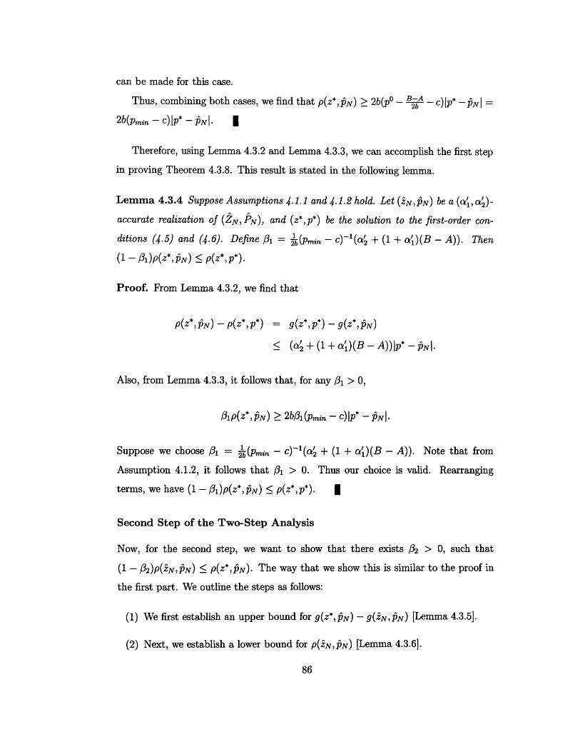
can be made for this case.

Thus, combining both cases, we find that p(z*, ^N) > 2b(po B - c)Ip* - PNI =

2b(pmin - c) Ip* - gNI I

Therefore, using Lemma 4.3.2 and Lemma 4.3.3, we can accomplish the first step

in proving Theorem 4.3.8. This result is stated in the following lemma.

Lemma 4.3.4 Suppose Assumptions 4.1.1 and 4.1.2 hold. Let (^N,P N) be a (a',,a')-

accurate realization of (ZN, iPN), and (z*,p*) be the solution to the first-order con-

ditions (4.5) and (4.6). Define p1 = -(pmin - c)-'(ac + (1 + a1)(B - A)). Then

(1 - 13 )p(z*, Ng) : p(z*,p*).

Proof. From Lemma 4.3.2, we find that

p(z*,jN) - p(z*,p*) =- g(z*,gN)

• (a' + (1 + a')(B - A))Ip* - NI-.

Also, from Lemma 4.3.3, it follows that, for any 01 > 0,

31 p(z*, PN) 2b,3l(Pmin - c) p* -4NI.

Suppose we choose 31 = ~(pmir - c)-1(a2 + (1 + a')(B - A)). Note that from

Assumption 4.1.2, it follows that 3P > 0. Thus our choice is valid. Rearranging

terms, we have (1 - 3 1)p(z*,PN) < p(z*,p*). I

Second Step of the Two-Step Analysis

Now, for the second step, we want to show that there exists 32 > 0, such that

(1 - 02)P(@N,PN) • p(Z* ,N). The way that we show this is similar to the proof in

the first part. We outline the steps as follows:

(1) We first establish an upper bound for g(z*,P-N) - g(£N, PN) [Lemma 4.3.5].

(2) Next, we establish a lower bound for P(iN,JN) [Lemma 4.3.6].

(3) By appropriately choosing 02, it follows that (1 - 02)P(N,1 N) < p(Z*, PN)

[Lemma 4.3.7].

Lemma 4.3.5 Let (zN, PN) be a (a', a') -accurate realization of (ZN, PN), and (z*,p*)

be the solution to the first-order conditions (4.5) and (4.6). Then g(z*,P )--g(SN, iN) •

alPNIZ* - ZSN.

Proof. We know that g(z, p) is a concave function with respect to z. Therefore, the

following inequality holds

1gg(z*, P) - g(~N, N) • (~(N,N)(Z* - ZN).

Since (N,iPN) is (ac,a')-accurate, therefore 2(2N,PsN)[ < PiNar. Then it follows

that

g(z*,^N) - 9(iN,1N) •: a ZNz -- N. I

Lemma 4.3.6 Suppose Assumptions 4.1.1 and 4.1.2 hold. Also suppose that there

exists y > 0 such that 1 o - p0o <y and Pmin - 7 > c. Let ( PN,1N ) be a realization

of (ZN, PN), and (z*,p*) be the solution to the first-order conditions (4.5) and (4.6).

Then we have p(iN, 3N) > Imin 1-,l p y) NIZ* - iI).

Proof. Define h(z) = g(z, PN) = (PN - c)(a - bPN) - cz - ca + NE[min(z, E)]. Note

that h(z) is a concave function. Also define the function f(z) = (fiN - c)(a - bpN) -

cz + 1N min(z, p). By Jensen's inequality, we know that E[min(z, E)] 5 min(z, t).

Therefore, f(z) > h(z) for all z.

Note that

f(z) (= N - c)(a - bfN + z), if z < /,

S(PN - c)(a - bPN) + PNI - CZ, if Z > U.

Let za be the intersection of y = h(iN) with y = (ON - c)(a - bfN + z), and zb be

its intersection with y = (fiN - c)(a - bPN) + PNI - CZ. Since f(z) Ž h(z) and both

functions are concave, then it is easy to verify that Iz* - SN I < zb - za.

The maximum of f(z) is achieved when z = i. And since f(z) Ž h(z) for all z,

then f (p) > h(iN). Also note that

f() - h(N) = (N - c)( - za),

f(p)- h(ZN) = C(Zb -).

Therefore, since we know that zb - za N Iz* - ^N , it follows that

1 1 c c)f(p) - h(•N) > - min(pN - c, C)(Zb - a) min • 1- NIZ* -- ZN

Also, from Proposition 4.2.1, we know that 3N A _< pO + y and PN > 3 p +

Pmin - Pmin - 7. Therefore,

1 c cf(y) - h(gN) > min +( , 1 P- - NZ* - ZNI.

2 po+ Pmin - Y)

Since c < PN 5 Pmax, then f (p) = (~ N-c)(a-bgN + A) 5 (Pmax--c)(a--b IY+p

(Pmax - c)(a - bc + yI). Therefore, it follows that

P(zN,PN) = (Pmax - c)(a - bc + p) - g(N, PN)

Sf (p) - h(iN)1 min 1 c z * - .

2-- pO + - Pmin - 7)

Lemma 4.3.7 Suppose Assumptions 4.1.1 and 4.1.2 hold. Also suppose that IPoN -

p0o_ -y, where y > 0 such that pmin - - > c. Let (iN, PN) be a (al, a')-accurate real-

ization of (ZN, PN), and (z*,p*) be the optimal solution to price-setting newsvendor

problem (4.4). Define 32 = 2a i min (-•7, 1 C- • ). Then (1-02)p(iNPN) <

p(z*,3 N).

Proof. From Lemma 4.3.5, we find that

P(N,<N) - p(z*,.N) = g(z*,N) - g(N,N)

ScalPNIZ* - Zn.

Also, from Lemma 4.3.6, it follows that, for any /2 > 0,

2 (p + 7 Pmin - )/2P(ZN'1pN)- m

Suppose we choose 82 = 2 [min ( 1 - . Note that since Pmin -

y > c, we have /2 > 0. Thus, our choice is valid. Rearranging terms, we have

(1 - 02)P(ZN, N) • p(z*, PN). I

Using Lemma 4.3.4 and Lemma 4.3.7, we can now prove Theorem 4.3.8 which

shows that if a policy (sN, PN) is (a/ , ca)-accurate, then the relative error of its regret

is bounded.

Theorem 4.3.8 Suppose Assumptions 4.1.1-4.1.3 hold. Suppose that i5o -p0 1 •< y,

where > 0 such that Pmin - > c. Let (ZN,1 3 N) be a (al,a'2)-accurate realization

of (ZN, PN), and (z*, p*) be the optimal solution to price-setting newsvendor problem.

Define 31 = (Pmin-c)- (a'+(1+a')(B-A)), /2 = 2a [min p• -, 1 pC_- )-

and a = (1-1)(1-2) - 1. If 31 < 1 and /2 < 1, then P(&N, N) < (1 + a)p(z*,p*).

Proof. Since /1 < 1 and /32 < 1, then from Lemma 4.3.7, we have

(1 - 01)(1 - ,2)P(2^N,jN) _ (1 - /1)p(z*,fiN).

And since from Lemma 4.3.2, we have

(1 - 01)p(z*, 6N) 5 p(z*,z*),

then it follows that (1 - 01)(1 - /2)P(@N,1N) < p(z*,p*). Therefore, if we define

O --- (1-)(1--2)l - 1, then P(iN,13 N) _ (1 + a)p(z*, p*). *

Theorem 4.3.8 establishes the relationship between (al, 2a)-accuracy and bounds

on the relative error of the regret for the solution to the data-driven approximation to

the first-order conditions. Note that the theorem holds if (ýN, 1N) is (a', a')-accurate

and po - il < 7y (or equivalently, lp - ft0 < 2by). Intuitively, the probability that

these conditions hold increases by taking more samples of the stochastic variable. The

next section establishes the connection between the sample size and the conditions

for which Theorem 4.3.8 hold.

4.3.2 Sample Size to Ensure First-Order Accuracy of the So-

lution to the Simulation-Based Procedure

In this subsection, we establish a relationship between the sample size of the data-

driven approximation to the first-order conditions and the first-order accuracy of its

solution. We will be using Hoeffding's inequality (see Theorem 2.3.4). The following

lemma states this relationship.

Lemma 4.3.9 Suppose Assumption 4.1.1 holds. For each a', a' > 0 and

0 < 6 1,62 < 1 such that 0 < 61+62 < 1, if the number of samples is N > max(Ni, N 2),

where

(B - A)2 og (2N2 = log2 2a1 (2(pmaz - c)

N2 = 2 2 log 2 C)

then the solution to the data-driven approximation to the first-order conditions (ZN, PN)

is (a', a'2)-accurate with probability of at least 1 - 61 - 62.

Proof. Note that each given sample of size N of the random component e implies a

(ZN, PN) that solves the system of linear equations (4.13) and (4.14). Define the event

B =F(N) < 1 - - .N

B(1p) = F(N) < 1 - C"-N -O a p5N =1 p •

I Ns

Define the quantile

z(itN) = inf z F(z) = 1 - N- - a

Since F(-) is nondecreasing, then B(fv) = [ZN < zl (f)I IgPN = Pil.

Since (ZN, izN) satisfies the data-driven approximation of the first-order conditions,

then conditional on PN = PN, we have FN(iN) = 1 - + Thus, since FN() is

nondecreasing, we have

Pr(B(j3y)) = Pr (ý < z1(•')LiN = N)

SPr (zl()) 1 - PN =).

Using Bayes Theorem,

PrPr (B(Z1 N PIN)Pr(B(r)) (z ))

Pr (1N = ~N)

From the definition of zl (ftN), we have

Pr • (•())- F(zl( t)) aPr(B(fjN)) Pr (PN = fiN)

exp(-2Na, 2)Pr (PN = PN)

where the last inequality follows from Hoeffding's inequality. Therefore, by choosing

N > ' log 2(pm62-c) ) we have Pr(B(IN)) Pr1 ')1Q 1 bl 2(Pma--C) pr(PN=P•N) "

With this choice of the sample size, since c < ^<N - Pmax, note that

Pmax

B) P) = Pr(B()) Pr (PN = pA) dpIN

Spmax d = 6 (4.22)c 2 (pmax - c) N 2

91


L = [F(iN) >1---PN

+ ,.

We can do the same analysis as we did for event B and apply Hoeffding's inequality.

Choosing N > log 2(Pm•-c)), we have Pr(L) = -


T = [LN[min(z, E)] - E[min(z, e)] > a] ,

where EN[min(z, E)] is given by equation (4.17). Consider the random variable Xk =

1(Ek • z) k + 1(ck > z)z. Note that EN[min(z, e)] = k EZ I Xk. Since A < Xk< B,

and

E[Xk] = Pr(E < z)E[EIE < z] + Pr(E > z)E[zlE > z]

= Pr(E < z)E[min(z, e)[e < z] + Pr(e > z)E[min(z, E)IE > z]

= E[min(z, e)],

then we can apply Hoeffding's inequality. Therefore,

Pr(T) = Pr (tN[min(z, e)] - E[min(z, e)] > a) <

Thus, if we choose N> (B-A log then Pr(T) < .2a- 62/) • ,h P(_ 2.


V = [E[min(z, e)] - EN[min(z, )] > a;].

We follow an analysis similar to that for event T and apply Hoeffding's inequality,

we find that for N> (BA)2 log (), we have Pr(V) <•2 • 2"

e-2 2N/(B-A)2

Therefore, if we choose

N > max (B - A2g , 2 1 log2a'2 I22' 61

then we find that

Pr(B U L U T U V) < Pr(B) + Pr(L) + Pr(T) + Pr(V)

S61+ 62-

Thus, it follows that Pr {(ZN, PN) is (a', a)-accurate} 1 - 6 - 62.

Before we can combine the results from Theorem 4.3.8 and Theorem 4.3.9, note

that an additional assumption for Theorem 4.3.8 is that jo _ p0o < y, for some 7 > 0.

Therefore, we first need the following lemma.

Lemma 4.3.10 Suppose Assumption 4.1.1 holds. For each 7 > 0 and 0 < 63 < 1,

if the number of samples is N > N3 = B 52 log , then po ° - ] < -y with

probability of at least 1 - 63.

Proof. Suppose there are N samples of E, given by 1,..., EN. Define

k a + bc + ek2b '

where E[Xk] __ a+b pO. Note that 0o = EkN X k . Since Xk E [a, 13] where

we define a = ++A and 3 = a+,+B then we can apply Hoeffding's inequality to

find

Pr(io -pO > Y) 5 exp (-22N exp (-b2() - a)2 (B - A)2

Thus, choosing N 2 log , then it follows that

Pr(PO - p0 > < 632

We can perform a similar proof for the probability that Po' - po0 -7y. Therefore,

we have for N> (B-A)2 log () that

Pr(po - ioI < y) I - 63.

The main result of this chapter is the following Theorem:

Theorem 4.3.11 Suppose Assumptions 4.1.1-4.1.3 hold. Further suppose that there

exists some y > 0 such that Pmin - 7 > c. Consider the price-setting newsvendor

problem specified by a unit cost c and a demand D(p, e) = a - bp + e, where e is

the random component. Let 0 < P31, 2 < 1 be specified accuracy levels such that

a= 1 - 1 E (0, 1], and 0 < 6 < 1 (for 0 < 6 < 1)be a specified confidence

level. Suppose for the choice of accuracy levels, the following condition holds:

C'2 - 2b/3 (pmin - c) - (1 + al)(B - A) > 0,

where1 c ca I 3 2 m2in , 1 -.2 p + 7 Pmin - 7

Suppose the data-driven approximation to the first-order conditions is solved with

respect to N i.i.d. samples of e, and that N > max(N1 , N2, N3 ), where

N1-- (B - A)2 og

N = log 5(Pmax - c)N2 : 2 log ,

S- (B - A)2 ) 58b2 2 6

Let (ZN, PN) be the solution to the data-driven approximation to the first-order con-

ditions and let (N, PN) be denote its realization. Then, with probability at least 1 - 6,

the regret of (ZN, PN) is at most 1 + a times the regret of an optimal solution (z*,p*)

to the price-setting newsvendor problem. In other words, P(zN, PN) < (1 + a)p(z*, P*)

with probability of at least 1 - 6.

Proof. Since Assumption 4.1.2 holds, then there exists some 7 > 0 such that Pmi -

y > c. Let 61 = J, 52 = • and 63 = . From Lemma 4.3.10, we know that for

N> N3

Pr (1oN - p > 7) < 63.

Also from Lemma 4.3.8, we know that for N > max(N1, N2),

Pr ((2N, PN)is not(a', a')-accurate) _ c, + 62.

Thus, we have for N > max(N 1, N2 , N3 )

Pr((2N,PN) is (a, a'c)-accurate and I| ° -p01 < 7y)

> 1 - Pr((ZN, PN) is not (a, a')-accurate)

-Pr(IPoN -P01 > 7) 1 - 51 - 2 - 63 = 1 -

From Theorem 4.3.8, we know that if 1 •o - p1 < 7y and if (SN, PN) is (a', a')-

accurate, then p(N, P15N) 5 (1 + a)p(z*,p*), where (z*,p*) is the solution to the

first-order equations. Moreover, under Assumptions 4.1.2-4.1.3, we know that the

first-order conditions (4.5) and (4.6) are uniquely solved by the optimal solution of

the price-setting newsvendor. Thus, we have for N > max(N 1 , N 2, N 3) the solution

to the data-driven approximation of the first-order conditions satisfies

Pr(p(2N, PN) (1 + a)p(z*, p*)) > 1 - 6,

where (z*,p*) is the optimal solution to the price-setting newsvendor problem. I

Theorem 4.3.11 outlines a procedure to choose a sample size that guarantees that

the regret of the solution to the data-driven approximation to the first-order condi-

tions satisfies a specified accuracy level with a specified confidence level. Compared to

the bound derived for the classical newsvendor problem in Theorem 2.3.6, note that

in the above theorem, accuracy depends on two parameters f1 and /2. The introduc-

tion of these two parameters correspond to accuracy in each of the two dimensions

(i.e., z and p).

NI and N2 are the bounds needed to ensure that (N, PN) is (a', a')-accurate with

high probability. On the other hand, N3 ensures that the sample size is large enough

such that the true mean p and the sample mean A are y-close with high probability.

Note that N2 is similar to the Hoeffding bound for the classical newsvendor problem,

except for the term pmax - c. This term appears, because unlike in the classical model,

p* (and IN) is not fixed and belongs to a range [c, pmax]. Similarly, note that the term

(B - A) in N3 appears because z* and zN belong in the range [A, B].

Chapter 5

Numerical Results for the

Data-Driven Price-Setting

Newsvendor Problem

In Chapter 4, we described a simulation-based procedure proposed by Zhan and

Shen [42] for solving the price-setting newsvendor problem if the explicit demand

distribution is not known. Under their model, the demand is composed of a deter-

ministic component and a random component. The deterministic demand is assumed

to be a linear function of the price with known parameters. That is, the stochastic

demand is D(p, e) = a - bp + E, where a is the zero-price demand level, b is the price-

sensitivity parameter and e is the random component. Under the simulation-based

approach, it is assumed that a set of N independent samples of the demand is avail-

able. In Chapter 4, we prove under certain assumptions on the random component

of the demand (e.g., boundedness) that the sample size is related to the accuracy

of the regret achieved by the solution to the procedure with respect to the optimal

regret computed with respect to the true distribution. However, the bound is only a

worst-case bound on the number of samples required. Moreover, bounded accuracy

may also be achieved for distributions that violate the assumptions in Chapter 4.

In this chapter, we conduct computational experiments to evaluate the perfor-

mance of the simulation-based procedure under various concrete scenarios. In partic-

ular:

* We explore how the simulation-based procedure performs as the unit cost c

varies.

* We explore how the simulation-based procedure performs as the zero-price de-

mand level a varies.

* We explore how the procedure performs as the price-sensitivity parameter b

varies.

* We explore the sensitivity of the procedure to different parameters of concrete

distributions.

The remainder of the chapter is outlined as follows. In Section 5.1, the experi-

mental design is described for the various computational experiments. In Section 5.2,

the results of the experiments are presented and discussed.

5.1 Methodology

We outline the steps of the simulation-based procedure by Zhan and Shen [42] as we

apply it in our numerical experiments.

* Obtain a set of N samples E1,..., 'N from the true demand distribution (see

pg. 78 on how to obtain these samples from demand-price data).

* Perform a gradient search with initial guess (^, Po), where ^ is a guess on the

expected value of the random component and Po is a guess on the optimal

riskless price (see pg. 75 for definition). We outline the gradient procedure:

1: Set tolerance level, Je

2: Set (Zold, Pold) " (A),P 0)

3: loop

4: Compute dz = -c + Pold 1 ( - E-i 1(Ek < Zold)

5: Compute dp = a + bc - 2bpold + -E NI=1min(Ek, Zold)

6: Choose stepsize s by Armijo rule

7: Set Znew Zold + s dz

8: Set Pnew Pold + S dp

9: if (zozld - new) 2 + (Pold - new )2 < 6J. then

10: Stop the loop

11: else

12: Set (Zold,Pold) -- (Znew,Pnew)

13: end if

14: end loop

* The first two steps are repeated for a total of m times.

The optimal solution to the SAA counterpart with N samples, (ZN, PN), is a ran-

dom variable that is dependent on the specific N samples of the random component

of demand E. The procedure outlined above is done for a total of m times to approx-

imate a distribution for (ZN, PN). Note also that different stepsize selection schemes

can be adopted, such as Armijo rule or diminishing stepsize rule (see Bertsekas [7] for

more details on stepsize selection). In these numerical examples we will be adopting

an Armijo stepsize selection rule.

In the experiments, we take N = 100 samples for m = 100 runs of the procedure.

We generate data from four distributions: uniform, normal, exponential, Pareto and

Poisson. In the base case, the zero-price demand level a = 200, the price-sensitivity

parameter b = 35 and the unit cost c = 1. The specifications of the distributions of

the base case are as follows:

Uniform range of [-10, 2jp + 10] with IL = 10

Normal mean p = 10 and standard deviation a = 25

Exponential mean , = 10

Pareto mean p = 10 and range [1, 00)

In analyzing the influence of the unit cost c, we consider various unit costs c. We

take c E [1, 1.5,..., 4].

In analyzing the influence of the zero-price demand level a, we consider a E

[100,200,..., 1000].

In analyzing the influence of the price-sensitivity parameters b, we take b E

[10, 15,. .. ,50].

The sensitivity analysis of the simulation-based procedure to various parameters

of concrete distributions is performed with the following specifications

Uniform p E [10, 20, ... , 100]

Normal pL E [10, 20,..., 100]

a E [10, 15,...,50]

Exponential p E [10, 20, ... , 100]

Pareto k E [2,3,...,50]

Since the distributions are not all bounded, we need to define a new regret function.

In this chapter, the regret function we consider is p(z, p) = (pO - c)(a - bc + p) -

g(z,p), where po is the riskless optimal price and g(z,p) is the expected profit. The

performance of the simulation is evaluated by observing the relative error of the

average expected profit and average regret. In particular, if (pk, p ) is the solution

to the simulation-based procedure for the kth run for k = 1,..., m, then

g(z*,p*) 1Average Relative Error of the Expected Profit = (*,*)g(z*, p*)

I E 1 p(ik, pk)- p(z*,p*)Average Relative Error of the Regret = p(z*,p* )

p(z*,p*)

where (z*, p*) is the optimal ordering and pricing policy under full knowledge of the

distribution.

5.2 Results and Discussion

In this section, we present the results of our computational experiments. We also

discuss these results and mention insights gained from the experiments.

100

Sensitivity to the Unit Cost

Figure A-12 plots the relative error in the expected profit and the regret achieved by

the SAA solution as a function of the unit cost. We make the following observations:

* From Figure A-12, we can observe that the relative error in the expected profit

and the regret achieved by the SAA solution is increasing against c for most

of the distributions. The relative error achieved by the Pareto distribution is

relatively invariant against c.

* We also observe that the relative error of the regret and the relative error of the

expected profit are highly correlated as c varies.

* The largest relative error of the expected profit is of the order 10-'. On the

other hand, the largest relative error of the regret is of the order 10-2.

Sensitivity to the Zero-Price Demand Level

Figure A-13 shows the relative error of the regret and the expected profit as a function

of the zero-price demand level a. We make the following observations:

* We can observe a decreasing trend in the relative error of the expected profit

achieved by the SAA counterpart as the zero-price level increases (Figure A-

13(a)). A similar decreasing trend can be observed for the relative error of the

regret (Figure A-13(b)). Again, the relative error of the Pareto distribution is

relatively consistent under different values of a.

* The relative error of the expected profit and the regret are highly correlated as

a varies.

* In both the regret and expected profit of the SAA solution, the relative error is

small (less than 10-2).

101

Sensitivity to the Price-Sensitivity Parameter

Figure A-14 plots the relative error in the expected profit and the regret achieved by

the SAA solution as a function of b.


* The relative error in the expected profit and the regret of all distributions except

Pareto exhibit an increasing trend as the price-sensitivity b increases. Pareto

on the other hand exhibits an opposite and decreasing trend.

* The relative error of the regret and the relative error of the expected profit

exhibit high correlation as b is varied.

* The relative errors of the expected profit and regret are at most of the order

10- 3

Sensitivity to Parameters of the Distribution

Figure A-15 plots the relative error of the regret and the expected profit of the SAA

solution as a function of the mean p of a uniform distribution.

Figure A-16 plots the relative error of the regret and the expected profit of the

SAA solution as a function of the mean p of an exponential distribution.


SAA solution as a function of the mean p of a normal distribution.


SAA solution as a function of the standard deviation a of the normal distribution.


SAA solution as a function of the parameter k of the Pareto distribution.


* The relative error of the regret and the expected profit are both exhibit an

increasing trend as the following distribution parameters are increased: p of the

uniform distribution (Figure A-15), p of the exponential distribution (Figure A-

16), and a of the normal distribution (Figure A-18).

102

* The relative error of the regret and of the expected profit exhibit a decreasing

trend for increasing: jt of the normal distribution and k of the Pareto distribu-

tion.

* In all experiments where the distribution parameters are varied, the relative

error of both the expected profit and regret are at most of the order 10- 3.

* There is a steep decreasing trend in the relative error (in regret and expected

profit) of the Pareto distribution for small values of k. Moreover, for k = 2

(where the variance is infinite), the relative error is less than 10- 4 . We can

infer that the simulation-based procedure performs well under an infinite second

moment.

* Again, the relative error in the expected profit and the relative error in the regret

exhibit high correlation for all the computational experiments where demand

parameters are varied.

From our discussion and observations, we can conclude that, unlike the SAA

approach for the classical newsvendor problem, the performance of the simulation-

based approach is highly dependent on the model parameters. Also, from the high

correlation between the relative error of the regret and the expected profit, we can

infer that the accuracy with respect to the expected profit is a valid criterion for a

good quality solution.

103

104

Appendix

Figures

A

105

1'

1(

I

0 0.2 0.4 0.6 0.8 1Critical Fractile, X

Figure A-1: The sample average of the error of the SAA order quantity as a functionof the critical fractile A.

106

2

a}0.aC

2a,CDcc

0.1 0.2 0.3 0.4 0.5 0.6 0.7 0.8 0.9Critical Fractile, X

(a) Relative Error of the Average expected profit of the SAA order quantity

10-1

10-2 1

10-3

10 -4

0.1 0.2 0.3 0.4 0.5 0.6Critical Fractile, X

0.7 0.8 0.9

(b) Relative Error of the Average Regret of the SAA order quantity

Figure A-2: The accuracy level achieved by the sample average expected profit andthe sample average regret of the SAA order quantity as a function of the criticalfractile A for various distributions.

107

-E- uni-+--- norm---- exp

- pareto- --- poiss

" S•• ..

I I I I I i I I I

10-12a)

C)

-2 10-0

w

a: 10~

150 200 250


0-1

10-2

SfA-4

150 200 250


Figure A-3: The accuracy level achieved by the sample average expected profit andthe sample average regret of the SAA order quantity as a function of the mean P ofthe uniform distribution.

108

----- 1-0.9-E- )=0.5-+- A=0.1

-- E- =--0.9--E-- =-0.5-- +-- •=0o.1

I I I I

C !!!, - ý ! !!I

-~f~a~ ............... _

2 i•.=0.9-- e-- z=o.5----•-- Z=0.1

3

10- 4

i

10- 3

Iv

a) 10

2x

n 10

- 4

0 50 100 150 200 250


10- 1

2

2 10- 2

S10wLU

0;

10-3

I 0- 4

0 100 150 200 250


Figure A-4: The accuracy level achieved by the sample average expected profit andthe sample average regret of the SAA order quantity as a function of the mean u ofthe normal distribution.

109

-B- =-0.9--- --0.5

---+-- -=0.1

I

0 10 20 30 40


10-1

Z,0

I-a,20Nw

a,ca

10- 3

1 - 4

a


Figure A-5: The accuracy level achieved by the sample average expected profit andthe sample average regret of the SAA order quantity as a function of the standarddeviation a of the normal distribution.

110

---- X=0.9-E- X=--0.5-+-- Z=0.1

r

Iv

0.14

0.1

0.08

0.06

0.04

0.02

200


0.14

0.08

0.06

0.04

0.02

150 200


Figure A-6: The accuracy level achieved by the sample average expectedthe sample average regret of the SAA order quantity as a function of thethe exponential distribution.

111

O. r~Dzio poopnOa o-DDDI

B-A-- =0.9-e-G x=0.5

fI4I

profit andmean y of

F

E

-

-

-- -- --

i Il=VI i Il=V. I (

O-a~k6&l - I~a Bi~W

-

-

-

-

10-2

10

(D

aCD -3

L..

02

Ca0) -4M 10

10 20 30 40


10 - 1

10-2

10-4


Figure A-7: The accuracy level achieved by the sample average expected profit andthe sample average regret of the SAA order quantity as a function of the parameterk of the Pareto distribution.

112

-B-- k-0.9--- =0.5-+-- X=-0.1

0-3

4-ID

02

wb(D

d0-

Critical Fractile, X

(a) Uniform

0.1 0.2 0.3 0.4 0.5 0.6 0.7 0.8 0.9Critical Fractile, )

(b) Normal

Figure A-8: The relative error of the regret achieved byquantity and the SAA order quantity for the uniform and

the minimax regret ordernormal distribution.

113

10o .

'

10o.40.3

- 101S

10 .

100.1

loo.,

100* 1

100 1110

L 100.o9

10.072

a)

100 0110 0 1


(a) Exponential


(b) Poisson

Figure A-9: The relative error of the regret achieved by the minimax regret orderquantity and the SAA order quantity for the exponential and Poisson distribution.

114

. 20iI

1(

10

1


(a) Uniform

a,

0,

a,a,

0.1 0.2 0.3 0.4 0.5 0.6 0.7 0.8 0.9Critical Fractile, A

(b) Pareto

Figure A-10: The relative error of the regret achieved by the parameter-estimationorder quantity and the SAA order quantity for the uniform and Pareto distribution.

115

-1010

C 105

c

S100

1Ir

· In- •


(a) Exponential

0.1 0.2 0.3 0.4 0.5 U.b U..I U.S U.jCritical Fractile, X

(b) Poisson

Figure A-11: The relative error of the regret achieved by the parameter-estimation

order quantity and the SAA order quantity for the exponential and Poisson distrib-

ution.

116

I,

1.5 2 2.5 3 3.5 4Unit Cost, c

(a) Relative error of the average expected profit

1 1.5 2 2.5Unit Cost, c

3 3.5 4

(b) Relative Error of the average regret

Figure A-12: The accuracy level achieved by the sample average expected profit andthe sample average regret of the SAA order quantity as a function of the unit cost c.

117

1U

M

ic0.0)

0.X

w.1

Ci6

Iv

10

16

0)

10-

· ·

I m l

-1

j -2

|Ij

,I

- -- uni-- E- norm--t-- exp

pareto

.00 300 400 500 600 700 800 900 1000Zero-Price Level, a


200 300 400 500 600 700Zero-Price Level, a

800 900 1000


Figure A-13: The accuracy level achieved by the sample average expected profit andthe sample average regret of the SAA order quantity as a function of the zero-pricedemand a.

118

100 2

CD

a)00P

1 ia)cc

100

e n-2

^•-2I

IV

15 20 25 30 35 40Price Sensitivity, b


10- 2

10-3

10 15 20 25 30 351Price Sensitivity, b

40 45 50


Figure A-14: The accuracy level achieved by the sample average expected profitand the sample average regret of the SAA order quantity as a function of the price-sensitivity parameter b.

119

4- 2

E- uni---- norm--+-- exp---- pareto

15..20 .25. 30.35 40

10-3

1 "-4

1( 45

-- e- uni-E- norm- exp----- pareto

I I I -I I I

I ·

10- 4

.w

0

I I I I

c

IL I -·-w~--3

L-0I.

._-(DUS

x 10- 3

0

Figure A-15: The accuracy level achieved by the sample average expected profit andthe sample average regret of the SAA order quantity as a function of the mean /, ofthe uniform distribution.

120

0

C

a)

cc[I

>•

x 10-3

10 20 30 40 50 60 70 80 90 100

Figure A-16: The accuracy level achieved by the sample average expected profit andthe sample average regret of the SAA order quantity as a function of the mean p ofthe exponential distribution.

121

x 10-4

20 30 40 50 60 70 80 90 100

Figure A-17: The accuracy level achieved by the samplethe sample average regret of the SAA order quantity as

the normal distribution.

average expected profit anda function of the mean p of

122

A

a,

(D

Ir

x 10-3

10 15 20 25 30a

Figure A-18: The accuracy level achieved bythe sample average regret of the SAA orderdeviation a of the normal distribution.

35 40 45 50

the sample average expected profit andquantity as a function of the standard

123

10-4

O-S

> 10-

Cr

0 ".

0 10 20 30 40 50

Figure A-19: The accuracy level achieved by the sample average expected profit andthe sample average regret of the SAA order quantity as a function of the parameterk of the Pareto distribution.

124

Bibliography

[1] M. Ball and M. Queyranne. Toward robust revenue management: com-petitive analysis of online booking. Working paper, available at SSRN:http://ssrn.com/abstract=896547, 2006.

[2] A. Ben-Tal and A. Nemirovski. Robust convex optimization. Mathematics ofOperations Research, 23(4):769-805, 1998.

[3] F. Bernstein and F. Federgruen. Decentralized supply chains with competingretailers under demand uncertainty. Management Science, 51(1):18-29, 2005.

[4] S. N. Bernstein. Theory of Probability. Moscow, 1927.

[5] D. Bertimas and A. Thiele. A data-driven approach to newsvendor problems.2005. Working Paper.

[6] D. Bertimas and A. Thiele. A robust optimization approach to inventory theory.Operations Research, 54(1):150-168, 2006.

[7] D. P. Bertsekas. Nonlinear Programming. Athena Scientific, Belmont, MA,second edition, 1999.

[8] D. Bertsimas and M. Sim. The price of robustness. Operations Research,52(1):35-53, 2003.

[9] J. H. Bookbinder and A. E. Lordahl. Estimation of inventory reorder level usingthe bootstrap statistical procedure. IEE Transactions, 21:302-312, 1989.

[10] G. Cachon and C. Terwiesch. Matching Supply with Demand: An Introductionto Operations Management. Irwin - McGraw Hill, 2005.

[11] L. Chan, M. Shen, D. Simchi-Levi, and J. Swann. Coordination of pricing andinventory decisions: A survey and classification. In D. Simchi-Levi, D. Wu, andM. Shen, editors, Handbook of Quantitative Supply Chain Analysis: Modellingin the E-Business Era. Kluwer Academic Publishers, 2004.

[12] J. D. Dana and N. C. Petruzzi. Note: The newsvendor model with endogenousdemand. Management Science, 47(11):1488-1497, 2001.

125

[13] S. Eren and C. Maglaras. Revenue management heuristics under limited marketinformation: A maximum entropy approach. Presented at The 6th Annual IN-FORMS Revenue Management Conference, Jun 5-6, Columbia University, 2006.

[14] R. L. Ernst. A linear inventory model of a monopolistic firm. Ph.D. Dissertation,Department of Economics, University of California, Berkeley, CA, 1970.

[15] G. Gallego and I. Moon. The distribution free newsboy problem: Review andextensions. Journal of the Operational Research Society, 44(8):825-834, 1993.

[16] P. Glasserman and Y. C. Ho. Gradient Estimation via perturbation analysis.Kluwer Academic Publishers, 1991.

[17] G. A. Godfrey and W. B. Powell. An adaptive, distribution-free algorithm forthe newsvendor problem with censored demands, with applications to inventoryand distribution. Management Science, 47:1101-1112, 2001.

[18] W. Hoeffding. Probability inequalities for sums of bounded random variables.Journal of the American Statistical Association, 58:13-30, 1963.

[19] W. T. Huh and P. Rusmevichientong. Adaptive capacity allocation with censoreddemand data: Application of concave umbrella functions. Working paper, 2006.

[20] W. T. Huh and P. Rusmevichientong. A non-parametric asymptotic analysis ofinventory planning with censored demand. Working paper, 2006.

[21] S. Karlin and C. R. Carr. Prices and optimal inventory policy. In K. J. Arrow,S. Karlin, and H. Scarf, editors, Studies in Applied Probability and ManagementScience, pages 159-172. Stanford University Press, Stanford, CA, 1962.

[22] M. Khouja. The single-period (news-vendor) problem: literature review andsuggestions for future research. Omega, the International Journal of ManagementScience, 27:537-553, 1999.

[23] A. J. Kleywegt, A. Shapiro, and T. Homem-De-Mello. The sample average ap-proximation method for stochastic discrete optimization. SIAM Journal on Op-timization, 12:479-502, 2001.

[24] R. Levi, R. Roundy, and D. B. Shmoys. Provably near-optimal sample-basedpolicies for stochastic inventory control models. Cornell Working Paper, 2005.

[25] L. H. Liyanage and J. G. Shanthikumar. A practical inventory control policyusing operational statistics. Operations Research Letters, 33:341-348, 2005.

[26] E. S. Mills. Uncertainty and price theory. Quarterly Journal of Economics,

73:116-130, 1959.

[27] G. E. Monahan, N. C. Petruzzi, and W. Zhao. The dynamic pricing problem froma newsvendor's perspective. Manufacturing and Service Operations Management,6:73-91, 2004.

126

[28] G. Perakis and G. Roels. Regret in the newsvendor model with partial informa-tion. To appear in Operations Research, 2006.

[29] G. Perakis and G. Roels. Robust controls for network revenue management.Working Paper, 2006.

[30] N. C. Petruzzi and M. Dada. Pricing and the newsvendor problem: A reviewwith extensions. Operations Research, 47(2):183-194, 1999.

[31] E. L. Porteus. Stochastic inventory theory. In D. P. Heyman and M. J. So-bel, editors, Handbooks in OR & MS, volume 2, pages 605-652. Elsevier, NorthHolland, 1990.

[32] G. Raz and E. L. Porteus. A discrete service levels perspective to the newsvendormodel with simultaneous pricing. Stanford University Working Paper, 2001.

[33] G. Raz and E. L. Porteus. A fractiles perspective to the joint price/quantitynewsvendor model. Management Science, 52(11):1764-1777, 2006.

[34] L. J. Savage. The theory of statistical decisions. Journal of the American Sta-tistical Association, 46(253):55-67, 1951.

[35] H. Scarf. Bayes solution to the statistical inventory problem. Annals of Mathe-matical Statistics, 30(2):490-508, 1959.

[36] H. E. Scarf. A min-max solution to an inventory problem. In K. J. Arrow andS. Karlin and H. E. Scarf, editor, Studies in Mathematical Theory of Inventoryand Production, pages 201-209. Stanford Univerity Press, Stanford, CA, 1958.

[37] M. Schweitzer and G. P. Cachon. Decision bias in the newsvendor problemwith known demand distribution: Experimental evidence. Management Science,46(3):404-420, 2000.

[38] A. Shapiro. Monte Carlo sampling methods. In A. Ruszczyniski and A. Shapiro,editor, Stochastic Programming, volume 10 of Handbooks in operations researchand management science, chapter 6. Elsevier, 2003.

[39] G. T. Thowsen. A dynamic, nonstationary inventory problem for aprice/quantity setting firm. Naval Research Logistics Quarterly, 22:461-476,1975.

[40] T. M. Whitin. Inventory control and price theory. Management Science, 2:61-68,1955.

[41] E. Zabel. Monopoly and uncertainty. Review of Economic Studies, 37:205-219,1970.

[42] R. L. Zhan and Z. J. M. Shen. Newsvendor problem with pricing: Properties,algorithms, and simulation. In Winter Simulation Conference, pages 1743-1748,2005.

127

Documents

Data-Driven Revenue Management