Data driven computing by the morphing fast Fourier ... · with the morphing EnKF to assimilate changes in the position of the epidemic. Keywords: Data assimilation, FFT, EnKF, Epidemic

Procedia Computer Science 00 (2010) 1–9

Procedia ComputerScience

International Conference on Computational Science, ICCS 2010

Data driven computing by themorphing fast Fourier transform ensemble Kalman filter in

epidemic spread simulations

Jan Mandela,∗, Jonathan D. Beezleya, Loren Cobba, Ashok Krishnamurthya

aDepartment of Mathematical and Statistical Sciences,University of Colorado Denver, Denver, CO 80217-3364, USA

Abstract

The FFT EnKF data assimilation method is proposed and applied to a stochastic cell simulation of an epidemic,based on the S-I-R spread model. The FFT EnKF combines spatial statistics and ensemble filtering methodologies intoa localized and computationally inexpensive version of EnKF with a very small ensemble, and it is further combinedwith the morphing EnKF to assimilate changes in the position of the epidemic.

Keywords: Data assimilation, FFT, EnKF, Epidemic spread, Cell model, Covariogram2010 MSC: 65C05, 62L12, 60G35

1. Introduction

Starting a model from initial conditions and then waiting for the result is rarely satisfactory. The model is generallyincorrect, data is burdened with errors, and new data comes in that needs to be accounted for. This is a well-knownproblem in weather forecasting, and techniques to incorporate new data by sequential statistical estimation are knownas data assimilation [1]. The ensemble Kalman filter (EnKF) [2] is a popular data assimilation method, which is easyto implement without any change in the model. The EnKF evolves an ensemble of simulations, and the model onlyneeds to be capable of exporting its state and restarting from the state modified by the EnKF. However, the ensemblesize required can be large (easily in the hundreds), the amount of computations in the EnKF can be significant, speciallocalization techniques need to be employed to suppress spurious long-range correlations in the ensemble covariancematrix, and the EnKF does not work well for problems with sharp coherent features, such as the travelling wavesfound in epidemics and wildfires.

We propose a variant of EnKF based on the Fast Fourier transform (FFT), which reduces significantly the amountof computations required by the EnKF, as well as the ensemble size. The use of FFT is inspired by spatial statistic:FFT EnKF assumes that the state approximately a stationary random field, that is, the covariance between two pointsis mainly a function of their distance vector. Then the multiplication of the covariance matrix and a vector is a

∗Corresponding authorEmail address: [email protected] (Jan Mandel)

c⃝ 2012 Published by Elsevier Ltd.

Procedia Computer Science 1 (2012) 1221–1229

www.elsevier.com/locate/procedia

1877-0509 c⃝ 2012 Published by Elsevier Ltd.doi:10.1016/j.procs.2010.04.136

Open access under CC BY-NC-ND license.

Open access under CC BY-NC-ND license.

http://www.elsevier.com/locate/procedia

http://dx.doi.org/10.1016/j.procs.2010.04.136

http://creativecommons.org/licenses/by-nc-nd/3.0/

http://creativecommons.org/licenses/by-nc-nd/3.0/

J. Mandel et al. / Procedia Computer Science 00 (2010) 1–9 2

convolution. In addition, the morphing transform [3] is used here so that changes of the state both in position and inamplitude are possible.

The FFT EnKF with morphing is illustrated here for tracking a simulated epidemic wave. The use of data assimi-lation techniques can increase the accuracy and reliability of epidemic tracking by using the data as soon as they areavailable, and some applications of data assimilation in epidemiology already exist [4, 5]. The FFT EnKF with morph-ing has the potential to reduce complicated simulations and accurate real-time use of data to a laptop or a smartphonein the field.

For FFT EnKF in a wildfire simulation, see [6]. The Fourier domain Kalman filter (FDKF) [7] consists of theKalman filter used in each Fourier mode separately.

The covariance of a stationary random field can be estimated from a single realization by the covariogram [8],which can be computed efficiently by the FFT [9]. We propose to use the covariogram for an EnKF with an ensembleof one, which will be further developed elsewhere.

2. FFT EnKF

The EnKF approximates the probability distribution of the model state u by an ensemble of simulations u1, . . . , uN .Each member is advanced by the simulation in time independently. When new data d arrives, it is given as datalikelihood d ∼ N (Hu,R), where H is the observation operator and R is the data error covariance matrix. Now theforecast ensemble [uk] is combined with the data by the EnKF analysis [10]

uak = uk +CN HT

(HCN HT + R

)−1 (d + ek − Huf

k

), k = 1, . . . ,N, (1)

to yield the analysis ensemble[ua

k

]. Here, CN is an approximation of the covariance C of the model state, taken to

be the covariance of the ensemble, and ek is sampled from N (0,R). The analysis ensemble is then advanced by thesimulations in time again. In [11], it was proved that the ensemble converges for large N to a sample from the Kalmanfiltering distribution when all probability distributions are Gaussian. Of course, the EnKF is used for more generalcases as well.

When CN is the ensemble covariance, the EnKF formulation (1) does not take advantage of any special structureof the model. This allows a simple and efficient implementation [12], but large ensembles, often over 100, are needed[2]. In an application, variables in the state are random fields, and the covariance decays with spatial distance [8].Tapering is the multiplication of sample covariance term-by-term with a fixed decay function that drops off with thedistance. Tapering improves the accuracy of the approximate covariance for small ensembles [13], but it makes theimplementation of (1) more expensive: the sample covariance matrix can no longer be efficiently represented as theproduct of two much smaller dense matrices, but it needs to be manipulated as a large, albeit sparse, matrix. Randomfields in geostatistics are often assumed to be stationary, that is, the covariance between two points depends on theirspatial distance vector only.

The FFT EnKF discussed here uses a very small ensemble, but larger than one. We explain the FFT EnKF inthe 1D case; higher-dimensional cases are exactly the same. Consider first the case when the model state consists ofone block only. Denote by u (xi), i = 1, . . . , n the entry of vector u corresponding to node xi. If the random field isstationary, the covariance matrix satisfies C

(xi, x j

)= c(xi − x j

)for some covariance function c, and multiplication by

C is the convolution

v (xi) =n∑

j=1

C(xi, x j

)u(x j

)=

n∑

j=1

u(x j

)c(xi − x j

), i = 1, . . . , n.

After FFT, convolution becomes entry-by-entry multiplication of vectors, that is, multiplication by a diagonal matrix.We assume that the random field is approximately stationary, so we neglect the off-diagonal terms of the covariance

matrix in the frequency domain, which leads to the the following FFT EnKF method. First apply FFT to each member,uk = Fuk. Next, approximate the forecast covariance matrix in the frequency domain by the diagonal matrix with thediagonal entries given by

ci =1

N − 1

N∑

k=1

∣∣∣∣uik − ui

∣∣∣∣2, where ui =

1N

N∑

k=1

uik. (2)

1222 J. Mandel et al. / Procedia Computer Science 1 (2012) 1221–1229


Then define approximate covariance matrix CN by term-by-term multiplication · in the Fourier domain

u = CNv ⇐⇒ u = Fu, v = c • u, v = F−1v,(c • u)i = ciui.

When H = I and R = rI, the evaluation of (1) reduces to

uak = uk + c • (c + r

)−1 •(d + ek − u f

k

). (3)

In general, the state has more than one variable, and u, C, and H have the block form

u =

⎡⎢⎢⎢⎢⎢⎢⎢⎢⎢⎢⎣

u(1)

...u(n)

⎤⎥⎥⎥⎥⎥⎥⎥⎥⎥⎥⎦, C =

⎡⎢⎢⎢⎢⎢⎢⎢⎢⎢⎢⎣

C(11) · · · C(1M)

.... . .

...C(M1) · · · C(MM)

⎤⎥⎥⎥⎥⎥⎥⎥⎥⎥⎥⎦, H =

[H(1) · · · H(M)

]. (4)

Here, the first variable is observed, so H(1) = I, H(2) = 0,. . . , H(M) = 0, and (1) becomes

u( j),ak = u( j)

k +C( j1)N

(C(11)

N + R)−1 (

d + ek − u(1)k

), j = 1, . . . ,M, (5)

and in the frequency domain

u( j),ak = u( j)

k + c( j1) •(c(11) + r

)−1 •(d + ek − uk

). (6)

The cross-covariance between field j and field 1 is approximated by neglecting the off-diagonal terms of the samplecovariance in the frequency domain as well,

c( j1)i =

1N − 1

N∑

k=1

(u( j)

ik − u( j)

i

) (u(1)

ik − u(1)

i

), where u

(�)

i =1N

N∑

k=1

u(�)ik , � = 1, j. (7)

In the computations reported here, we have used the real sine transform, so all numbers in (7) are real. Also, theuse of the sine transform naturally imposes no change of the state on the boundary.

3. Morphing EnKF

Given an initial state u, the initial ensemble in the morphing EnKF [3, 12] is given by

u(i)k =(u(i)

N+1 + r(i)k

)◦ (I + Tk) , k = 1, . . . ,N, (8)

with an additional member uN+1 = u, called the reference member. In (8), r(i)k are random smooth functions on Ω,

Tk are random smooth mappings Tk : Ω → Ω, and ◦ denotes composition. Thus, the initial ensemble varies bothin amplitude and in position, and the change position is the same in all blocks. The random smooth functions andmapping are generated by FFT as Fourier series with random coefficients with zero mean and variance that decaysquickly with frequency.

The data d is an observation of u(1). The first blocks of all members u1, . . . , uN and d are then registered againstthe first block of uN+1 as

u(1)k ≈ u(1)

N+1 ◦ (I + Tk) , Tk ≈ 0, ∇Tk ≈ 0, k = 0, . . . ,N,

u(1)0 = d and Tk : Ω → Ω, k = 0, . . . ,N are called registration mappings. The registration mapping is found by

multilevel optimization. The morphing transform maps each ensemble member uk into the extended state vector, themorphing representation,

uk → uk = MuN+1 (uk) =(Tk, r

(1)k , . . . , r

(M)k

), (9)

where r( j)k = u( j)

k ◦ (I + Tk)−1 − u( j)N+1, k = 0, . . . ,N, are registration residuals. Likewise, the extended data vector is

defined by d → d =(T0, r

(1)0

)and the the observation operator is

(T, r(1), . . . , r(M)

)→(T, r(1)

). We then apply the



FFT EnKF method (6) is applied to the transformed ensemble u1, . . . , uN . The covariance C(11) in (5) consists of threediagonal matrices and we neglect the off-diagonal blocks, so the fast formula (6) can be used. The analysis ensembleu1, . . . , uN+1 is obtained by the inverse morphing transform

ua,(i)k = M−1

uN+1

(ua

k

)=(u(i)

N+1 + ra,(i)k

)◦(I + T a

k

), k = 1, . . . ,N + 1, (10)

where the new transformed reference member is given by

uaN+1 =

1N

N∑

k=1

uak . (11)

4. Epidemic model

The epidemic model that we used for this study is a spatial version of the common S-I-R dynamic epidemic model.A person is susceptible or infectious in this context if he or she can contract or transmit the disease, respectively. Theremoved state includes those who have either died, have been quarantined, or have recovered from the disease andbecome immune. The state variables are the susceptible (S ), the infectious (I), and the removed (R) populationdensities.The core ideas for this model date back to the 1957 spatial formulation by Bailey [14], but the specificversion that we have employed here is due to Hoppenstaedt [15, p. 64].

The population is considered to be dispersed over a planar domain Ω ⊂ R2, and it is labelled according to itsposition with respect to the spatial coordinates x and y. The (deterministic) evolution of the state (S (t) , I (t) ,R (t)) isgiven by

∂S (x,y,t)∂t = −S (x, y, t)

∫∫

Ω

w (x, y, u, v) I (u, v, t) dudv,

∂I(x,y,t)∂t = S (x, y, t)

∫∫

Ω

w (x, y, u, v) I (u, v, t) dudv − q (x, y, t) I (x, y, t) ,

∂R(x,y,t)∂t = qi (x, y, t) I (x, y, t) .

⎫⎪⎪⎪⎪⎪⎪⎪⎬⎪⎪⎪⎪⎪⎪⎪⎭(12)

The function q (x, y, t) gives the rate of removal of infectives due to death, quarantine, or recovery. The weightfunction w (x, y, u, v) measures the influence of infectives at spatial position (u, v) on the exposure of susceptiblesat position (x, y); in this simulation we used the function w (x, y, u, v) = α exp

[−((x − u)2 + (y − v)2)1/2/λ], which

expresses the idea that the influence of nearby infectives decays as an exponential function of Euclidean distance,with constant λ, characteristic of the distance at which the disease spreads. More mobile societies will have largervalues of λ. The parameter α measures the infectiousness of the disease.

A stochastic cell model is created by treating the quantities on the right-hand-side of (12) as the intensities of aPoisson process and by piecewise constant integration over the cells. The domain Ω is decomposed into nonover-lapping cells Ωi with centers (xi, yi) and areas A (Ωi), i = 1, . . . ,K. The state in the cell Ωi is the random element(S i, Ii,Ri), advanced in time over the interval [t, t + Δt] by

S i (t + Δt) = S i (t) − ΔS i, Ii (t + Δt) = Ii (t) + ΔS i − ΔRi, Ri (t + Δt) = Ri (t) + ΔRi,

where the random increments ΔS i and ΔRi are sampled from

ΔS i ∼ Pois(S i (t)

∑Kj=1w(xi, yi, x j, y j

)I j (t) A (Ωi)Δt

), (13)

ΔRi ∼ Pois (qi (t) Ii (t) A (Ωi)Δt) ,

and qi (t) is the given removal rate in the cell Ωi. The summation in (13) is done only over the cells Ω j near Ωi;for far away cells, the weights w

(xi, yi, x j, y j

)are negligible. It is not necessary to compute a Poisson-distributed

transmission rate from each source cell to a given target cell, because a finite sum of independent Poisson-distributedrandom variables, each with its own intensity parameter, is itself Poisson-distributed with an intensity parameter equalto the sum of the individual intensities.



(a) (b)

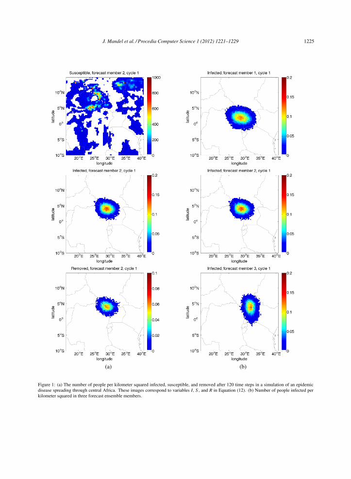
Figure 1: (a) The number of people per kilometer squared infected, susceptible, and removed after 120 time steps in a simulation of an epidemicdisease spreading through central Africa. These images correspond to variables I, S , and R in Equation (12). (b) Number of people infected perkilometer squared in three forecast ensemble members.



5. Computational results

We have chosen to model an epidemic disease that first emerges in Congo. The computational domain is a squareportion of central Africa. In Figure 1 (a), we see the epidemic wave 120 model time steps after the emergence of thedisease. The behavior of the model is such that any spurious infection will tend to grow into a secondary infectionwave. This is problematic for data assimilation because the occurrence of spurious features is virtually guaranteed.We attempt to reduce the occurrence and magnitude of these features using the morphing transformation and FFTEnKF; however, some amount of residual artifacts will remain. We have found that by processing the model state inthe following manner, we can further reduce these artifacts. We begin by scaling the absolute quantities containedin the model variables to a percentage of the local population before performing the data assimilation. After dataassimilation, we truncate the variables to the range [0, 1], and we apply a threshold so that any infection rate below1% is set to 0. Finally, we rescale the output in absolute units ensuring that the number of people at each grid cell ispreserved. We have applied the FFT EnKF to the epidemic model described in Section 4 with an ensemble of size 5.Each ensemble simulation was started with the same initial conditions, but with different random seeds, and advancedin time by 100 model time units, then perturbed randomly to obtain the initial ensemble. The analysis ensemble anddata were advanced in time an additional 20 model time steps for further assimilation cycles. In total, 3 assimilationcycles were performed in this manner.

We have perturbed each member of the initial ensemble randomly in space by applying (10) to the each variableof the morphing representation of the model. The mappings Tk for this perturbation were generated from a space ofsmooth functions that are zero at the boundary. While the residuals rk are customarily initialized to smooth randomfields as well, we have chosen to set rk = 0 to avoid spurious infections. We instead multiply each field after theinverse morphing transform by 1 + sk, where sk is another smooth random field. This ensures that an initial infectionrate of 0 is unchanged by the perturbation. A part of a typical ensemble with spatial as well as amplitude variability isshown Figure 1 (b).

The output of the observation function used in this example consists of the Infected field of the model. In this case,the data is a spatial “image” of the number of infected persons in each grid cell. The data were generated syntheticallyfrom a model simulation, which was initialized in the same manner as the ensemble.

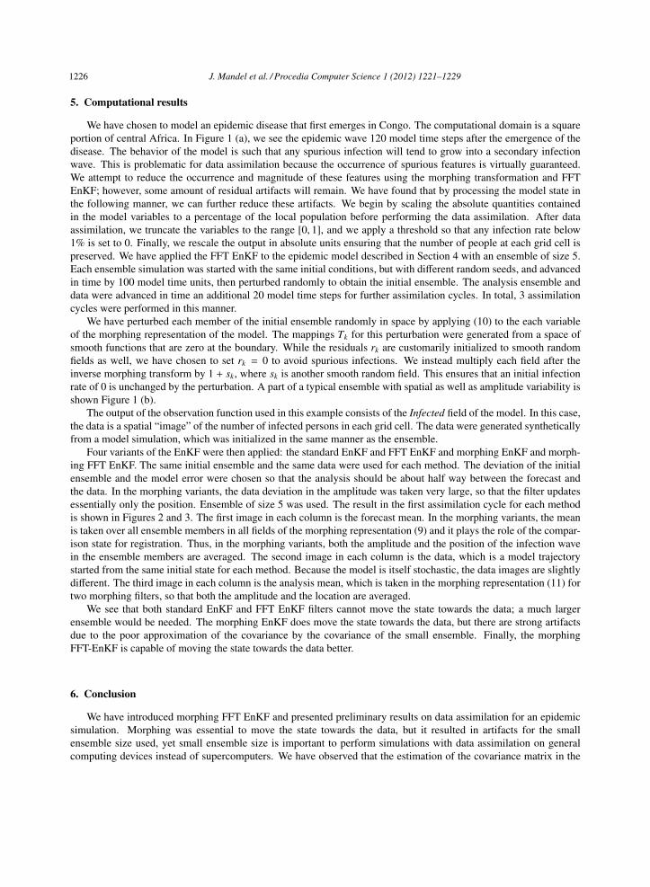
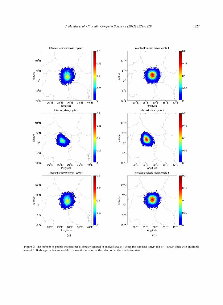
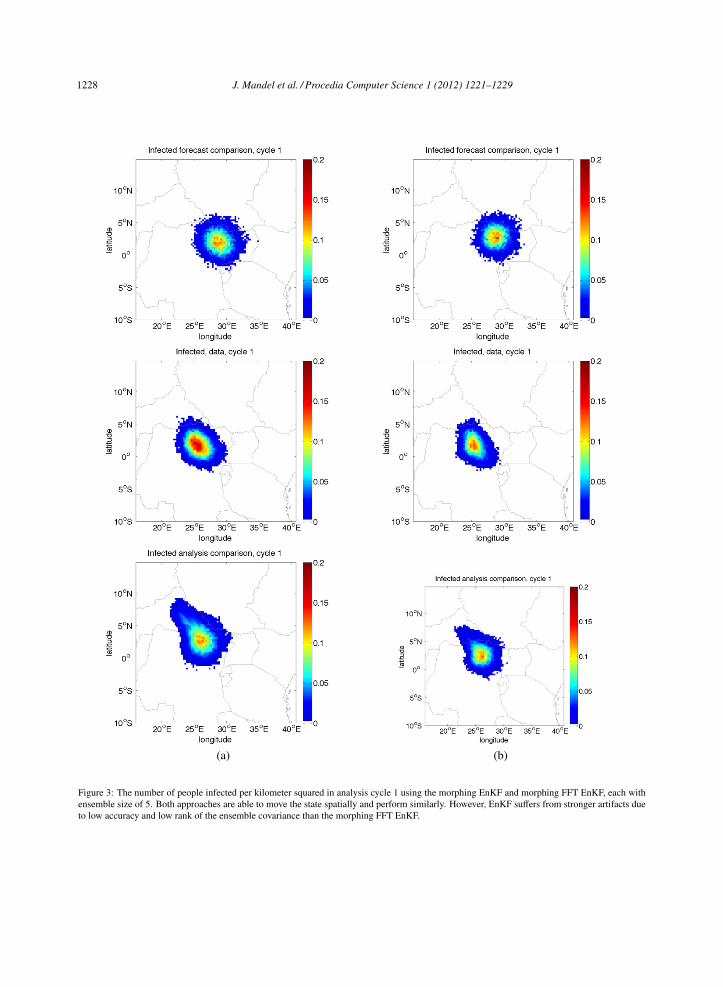
Four variants of the EnKF were then applied: the standard EnKF and FFT EnKF and morphing EnKF and morph-ing FFT EnKF. The same initial ensemble and the same data were used for each method. The deviation of the initialensemble and the model error were chosen so that the analysis should be about half way between the forecast andthe data. In the morphing variants, the data deviation in the amplitude was taken very large, so that the filter updatesessentially only the position. Ensemble of size 5 was used. The result in the first assimilation cycle for each methodis shown in Figures 2 and 3. The first image in each column is the forecast mean. In the morphing variants, the meanis taken over all ensemble members in all fields of the morphing representation (9) and it plays the role of the compar-ison state for registration. Thus, in the morphing variants, both the amplitude and the position of the infection wavein the ensemble members are averaged. The second image in each column is the data, which is a model trajectorystarted from the same initial state for each method. Because the model is itself stochastic, the data images are slightlydifferent. The third image in each column is the analysis mean, which is taken in the morphing representation (11) fortwo morphing filters, so that both the amplitude and the location are averaged.

We see that both standard EnKF and FFT EnKF filters cannot move the state towards the data; a much largerensemble would be needed. The morphing EnKF does move the state towards the data, but there are strong artifactsdue to the poor approximation of the covariance by the covariance of the small ensemble. Finally, the morphingFFT-EnKF is capable of moving the state towards the data better.

6. Conclusion

We have introduced morphing FFT EnKF and presented preliminary results on data assimilation for an epidemicsimulation. Morphing was essential to move the state towards the data, but it resulted in artifacts for the smallensemble size used, yet small ensemble size is important to perform simulations with data assimilation on generalcomputing devices instead of supercomputers. We have observed that the estimation of the covariance matrix in the



(a) (b)

Figure 2: The number of people infected per kilometer squared in analysis cycle 1 using the standard EnKF and FFT EnKF, each with ensemblesize of 5. Both approaches are unable to move the location of the infection in the simulation state.



(a) (b)

Figure 3: The number of people infected per kilometer squared in analysis cycle 1 using the morphing EnKF and morphing FFT EnKF, each withensemble size of 5. Both approaches are able to move the state spatially and perform similarly. However, EnKF suffers from stronger artifacts dueto low accuracy and low rank of the ensemble covariance than the morphing FFT EnKF.



frequency domain results in better forecast covariance in the algorithm, which has the potential to reduce the artifactsdue to small ensemble size.

7. Acknowledgements

This work was partially supported by NIH grant 1 RC1 LM01641-01 and NSF grants CNS-0719641 and ATM-0835579.

References

[1] E. Kalnay, Atmospheric Modeling, Data Assimilation and Predictability, Cambridge University Press, 2003.[2] G. Evensen, Data Assimilation: The Ensemble Kalman Filter, 2nd Edition, Springer Verlag, 2009.[3] J. D. Beezley, J. Mandel, Morphing ensemble Kalman filters, Tellus 60A (2008) 131–140.[4] L. Bettencourt, R. Ribeiro, G. Chowell, T. Lant, C. Castillo-Chavez, Towards real time epidemiology: data assimilation, modeling and

anomaly detection of health surveillance data streams, in: Intelligence and Security Informatics: Biosurveillance, Vol. 4506 of Lecture Notesin Computer Science, Springer, 2007, pp. 79–90.

[5] C. Rhodes, T. Hollingsworth, Variational data assimilation with epidemic models, Journal of Theoretical Biology 258 (4) (2009) 591–602.[6] J. Mandel, J. D. Beezley, V. Y. Kondratenko, Fast Fourier transform ensemble Kalman filter with application to a coupled atmosphere-wildland

fire model, arXiv:1001.1588, International Conference on Modeling and Simulation (MS’2010), accepted (2010).[7] E. Castronovo, J. Harlim, A. J. Majda, Mathematical test criteria for filtering complex systems: plentiful observations, J. Comput. Phys.

227 (7) (2008) 3678–3714.[8] N. A. C. Cressie, Statistics for Spatial Data, John Wiley & Sons Inc., New York, 1993.[9] D. Marcotte, Fast variogram computation with FFT, Computers & Geosciences 22 (10) (1996) 1175–1186.

[10] G. Burgers, P. J. van Leeuwen, G. Evensen, Analysis scheme in the ensemble Kalman filter, Monthly Weather Review 126 (1998) 1719–1724.[11] J. Mandel, L. Cobb, J. D. Beezley, On the convergence of the ensemble Kalman filter, arXiv:0901.2951, Applications of Mathematics, to

appear (January 2009).[12] J. Mandel, J. D. Beezley, J. L. Coen, M. Kim, Data assimilation for wildland fires: Ensemble Kalman filters in coupled atmosphere-surface

models, IEEE Control Systems Magazine 29 (2009) 47–65.[13] R. Furrer, T. Bengtsson, Estimation of high-dimensional prior and posterior covariance matrices in Kalman filter variants, J. Multivariate

Anal. 98 (2) (2007) 227–255.[14] N. Bailey, Mathematical Theory of Epidemics, Griffin, 1957.[15] F. Hoppenstaedt, Mathematical Theories of Populations, Demographics, and Epidemics, CBMS-NSF Regional Conference Series in Applied

Mathematics, SIAM, 1975.


Documents

Data driven computing by the morphing fast Fourier ... · with the morphing EnKF to assimilate changes in the position of the epidemic. Keywords: Data assimilation, FFT, EnKF, Epidemic