Data Analysis Using SPSS 15. - University of Sheffieldcics.dept.shef.ac.uk/userguides/spss15.pdf · are not part of the site license we have at Sheffield. ... Jean Russell, Bob Booth

Quantitative Data Analysis Using SPSS 15.

Jean Russell

Bob Booth

November 2008

AP-SPSS2

University of Sheffield

Jean Russell, Bob Booth Quantitative Data Analysis Using SPSS 15

2

Contents

1. INTRODUCTION ............................................................................................................................ 3

1.1 UNITS .................................................................................................................................................. 3 1.2 VARIABLES .......................................................................................................................................... 4

2. STARTING SPSS ........................................................................................................................... 5

2.1 THE HELP AVAILABLE IN SPSS ........................................................................................................... 6

3. ENTERING DATA INTO SPSS ...................................................................................................... 7

3.1 TYPING DATA INTO SPSS .................................................................................................................... 7 3.2 SAVING AND LOADING SPSS DATA ................................................................................................... 11 3.3 ENTERING DATA FROM AN EXCEL SPREADSHEET .............................................................................. 12 3.4 IMPORTING DATA FROM A TEXT FILE ................................................................................................ 13 3.5 IMPORTING DATA FROM A DATABASE ............................................................................................... 14

4. TRANSFORMING VARIABLES ................................................................................................... 16

4.1 COMPUTING VARIABLES .................................................................................................................... 16 4.2 RECODING VARIABLES ...................................................................................................................... 17

5. GRAPHS ...................................................................................................................................... 18

5.1 THE CHART BUILDER ........................................................................................................................ 18 5.2 CHART EDITOR .................................................................................................................................. 20

6. STATISTICAL TECHNIQUES ...................................................................................................... 21

6.1 SPSS STATISTICS OVERVIEW ............................................................................................................ 21 6.2 FREQUENCIES .................................................................................................................................... 22 6.3 CROSSTABS ....................................................................................................................................... 23 6.4 INDEPENDENT T-TEST ........................................................................................................................ 24 6.5 MANN-WHITNEY U TEST .................................................................................................................. 25 6.6 CORRELATIONS.................................................................................................................................. 26

7. ADVANCED ANALYSES ............................................................................................................. 27

7.1 ONE WAY ANOVA ............................................................................................................................ 27 7.2 TESTING FOR EQUALITY OF VARIANCE .............................................................................................. 28 7.3 FACTORIAL ANOVA (AND ANCOVA) ............................................................................................. 29 7.4 CHECKING THAT THE RESIDUALS ARE NORMALLY DISTRIBUTED ........................................................ 33 7.5 WHY STATISTICIANS PREFER GRAPHS TO TEST FOR CHECKING NORMALITY OF RESIDUALS ............. 34 7.6 LINEAR REGRESSION ......................................................................................................................... 35 7.7 LOGISTIC REGRESSION ....................................................................................................................... 37

8. INTERACTING WITH A WORD DOCUMENT ............................................................................. 39

8.1 PUTTING DATA TABLES IN WORD DOCUMENTS ................................................................................ 39 8.2 PUTTING GRAPHS IN WORD DOCUMENTS .......................................................................................... 39 8.3 EXPORTING TO WEB PAGE AND GRAPHICS FILES .............................................................................. 39

9. SYNTAX ....................................................................................................................................... 40

10. FURTHER READING ................................................................................................................... 40


3

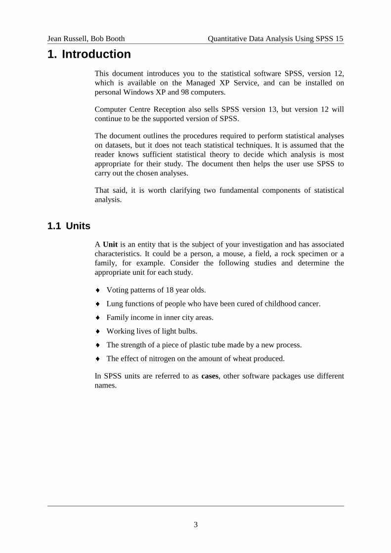
1. Introduction

This document introduces you to the statistical software SPSS, version 12,

which is available on the Managed XP Service, and can be installed on

personal Windows XP and 98 computers.

Computer Centre Reception also sells SPSS version 13, but version 12 will

continue to be the supported version of SPSS.

The document outlines the procedures required to perform statistical analyses

on datasets, but it does not teach statistical techniques. It is assumed that the

reader knows sufficient statistical theory to decide which analysis is most

appropriate for their study. The document then helps the user use SPSS to

carry out the chosen analyses.

That said, it is worth clarifying two fundamental components of statistical

analysis.

1.1 Units

A Unit is an entity that is the subject of your investigation and has associated

characteristics. It could be a person, a mouse, a field, a rock specimen or a

family, for example. Consider the following studies and determine the

appropriate unit for each study.

Voting patterns of 18 year olds.

Lung functions of people who have been cured of childhood cancer.

Family income in inner city areas.

Working lives of light bulbs.

The strength of a piece of plastic tube made by a new process.

The effect of nitrogen on the amount of wheat produced.

In SPSS units are referred to as cases, other software packages use different

names.


4

1.2 Variables

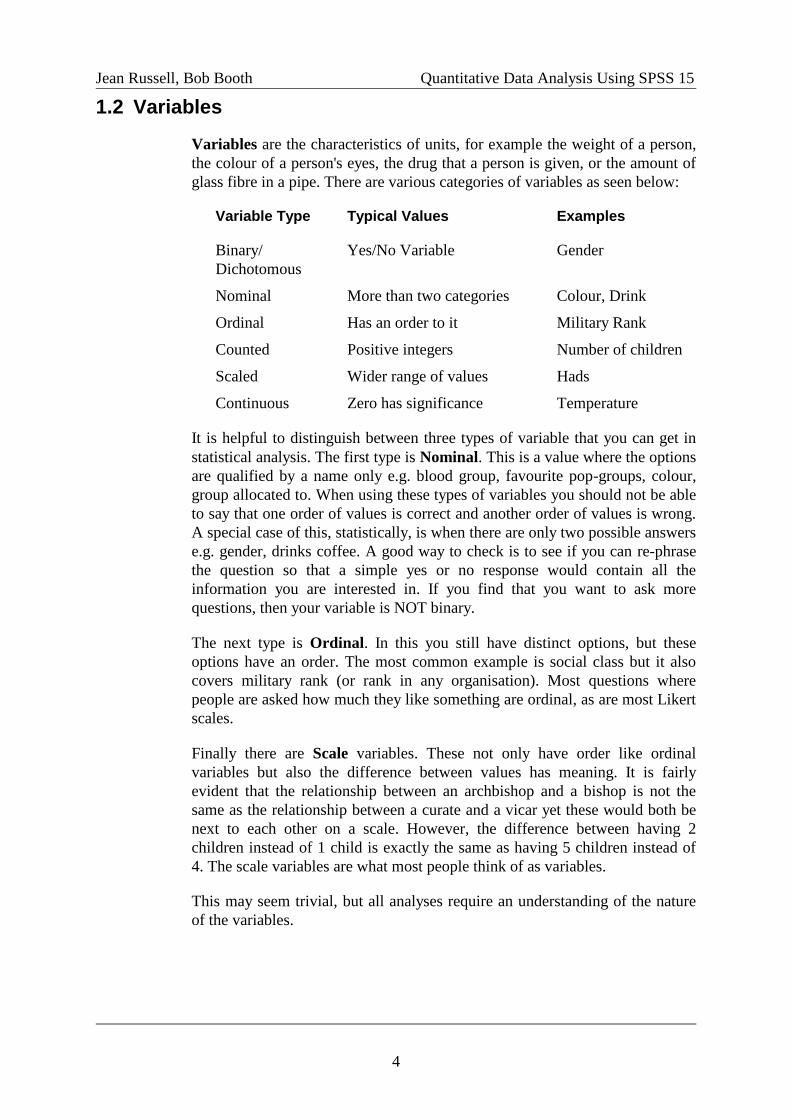
Variables are the characteristics of units, for example the weight of a person,

the colour of a person's eyes, the drug that a person is given, or the amount of

glass fibre in a pipe. There are various categories of variables as seen below:

Variable Type Typical Values Examples

Binary/ Yes/No Variable Gender

Dichotomous

Nominal More than two categories Colour, Drink

Ordinal Has an order to it Military Rank

Counted Positive integers Number of children

Scaled Wider range of values Hads

Continuous Zero has significance Temperature

It is helpful to distinguish between three types of variable that you can get in

statistical analysis. The first type is Nominal. This is a value where the options

are qualified by a name only e.g. blood group, favourite pop-groups, colour,

group allocated to. When using these types of variables you should not be able

to say that one order of values is correct and another order of values is wrong.

A special case of this, statistically, is when there are only two possible answers

e.g. gender, drinks coffee. A good way to check is to see if you can re-phrase

the question so that a simple yes or no response would contain all the

information you are interested in. If you find that you want to ask more

questions, then your variable is NOT binary.

The next type is Ordinal. In this you still have distinct options, but these

options have an order. The most common example is social class but it also

covers military rank (or rank in any organisation). Most questions where

people are asked how much they like something are ordinal, as are most Likert

scales.

Finally there are Scale variables. These not only have order like ordinal

variables but also the difference between values has meaning. It is fairly

evident that the relationship between an archbishop and a bishop is not the

same as the relationship between a curate and a vicar yet these would both be

next to each other on a scale. However, the difference between having 2

children instead of 1 child is exactly the same as having 5 children instead of

4. The scale variables are what most people think of as variables.

This may seem trivial, but all analyses require an understanding of the nature

of the variables.


5

2. Starting SPSS

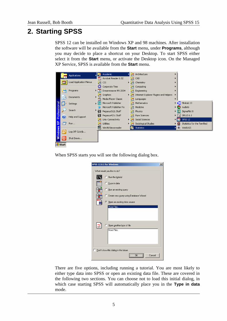
SPSS 12 can be installed on Windows XP and 98 machines. After installation

the software will be available from the Start menu, under Programs, although

you may decide to place a shortcut on your Desktop. To start SPSS either

select it from the Start menu, or activate the Desktop icon. On the Managed

XP Service, SPSS is available from the Start menu.

When SPSS starts you will see the following dialog box.

There are five options, including running a tutorial. You are most likely to

either type data into SPSS or open an existing data file. These are covered in

the following two sections. You can choose not to load this initial dialog, in

which case starting SPSS will automatically place you in the Type in data

mode.


6

2.1 The Help Available in SPSS

SPSS has a collection of help tools from the Help menu. Topics leads to the

normal help files that you find in all packages, containing information on how

to perform specific tasks, for example, how to declare a missing value.

However SPSS has several other forms of help available from the Help menu.

It has a Tutorial that is a basic introduction to SPSS, and covers very much the

same areas as the course. More advanced tutorials can be obtained, but they

are not part of the site license we have at Sheffield.

It also contains tools, called coaches, that require Internet Explorer. The

Statistics Coach will help you select the statistics to perform. Be wary of this

tool, as it may encourage type 3 errors (the correct answer to the wrong

question). The algorithm used is fairly simple. It will not consider all the

information known about the data prior to analysis, nor does it directly

consider the actual question you are asking. Therefore, it may suggest a variety

of analyses, no analysis, or even suggest an inappropriate analysis. Although it

can be useful, the Statistics Coach is no substitute for understanding statistical

tests or reading a textbook.

The Results Coach is more satisfactory. It is only available when you are

editing an output object, and will help you interpret the analysis. However, it

will take one line for interpretation when there are often a variety in the

literature. You will need the line that is commonly used in your subject.

There is also a Syntax Coach. This is different from the other coaches in that

it does not depend on Internet Explorer. It gives the command syntax for

SPSS. At present I recommend you ignore this option, though for the more

experience user, it is likely to be the part of the Help system that you use most

often.

Finally, if you select part of an output object and click the right mouse button,

a pop-up menu will appear. One of the options will be What is this? This will

give a definition of the item selected.


7

3. Entering Data into SPSS

3.1 Typing Data into SPSS

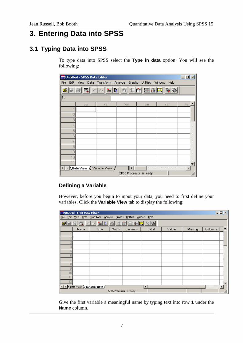
To type data into SPSS select the Type in data option. You will see the

following:

Defining a Variable

However, before you begin to input your data, you need to first define your

variables. Click the Variable View tab to display the following:

Give the first variable a meaningful name by typing text into row 1 under the

Name column.


8

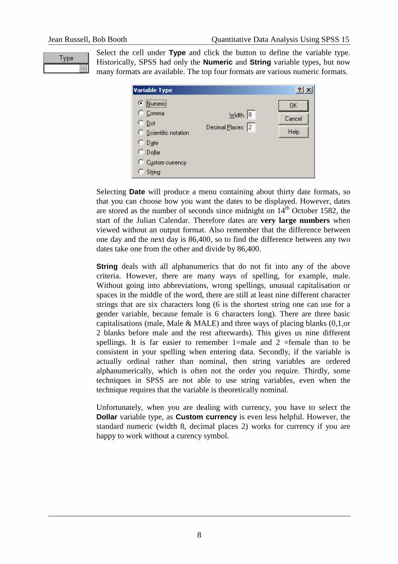
Select the cell under Type and click the button to define the variable type.

Historically, SPSS had only the Numeric and String variable types, but now

many formats are available. The top four formats are various numeric formats.

Selecting Date will produce a menu containing about thirty date formats, so

that you can choose how you want the dates to be displayed. However, dates

are stored as the number of seconds since midnight on 14th

October 1582, the

start of the Julian Calendar. Therefore dates are very large numbers when

viewed without an output format. Also remember that the difference between

one day and the next day is 86,400, so to find the difference between any two

dates take one from the other and divide by 86,400.

String deals with all alphanumerics that do not fit into any of the above

criteria. However, there are many ways of spelling, for example, male.

Without going into abbreviations, wrong spellings, unusual capitalisation or

spaces in the middle of the word, there are still at least nine different character

strings that are six characters long (6 is the shortest string one can use for a

gender variable, because female is 6 characters long). There are three basic

capitalisations (male, Male & MALE) and three ways of placing blanks (0,1,or

2 blanks before male and the rest afterwards). This gives us nine different

spellings. It is far easier to remember 1=male and 2 =female than to be

consistent in your spelling when entering data. Secondly, if the variable is

actually ordinal rather than nominal, then string variables are ordered

alphanumerically, which is often not the order you require. Thirdly, some

techniques in SPSS are not able to use string variables, even when the

technique requires that the variable is theoretically nominal.

Unfortunately, when you are dealing with currency, you have to select the

Dollar variable type, as Custom currency is even less helpful. However, the

standard numeric (width 8, decimal places 2) works for currency if you are

happy to work without a curency symbol.


9

In the Labels column, you can supply a label for the variable. This was

introduced as an aid to memory. When you just use variable names, without

variable labels, you are restricted to eight characters to describe the variable.

This is decidedly limiting and you end up with abbreviations such as q32a_m

or r_armlen. You then have to remember exactly what each abbreviation

stands for. Instead of having to rely on this, you can store a string of up to 256

characters with the data for the variable in SPSS. This description will often

appear when carrying out an analysis, and will be the label on the appropriate

axis for a graph.

If you are using a more recent version of SPSS, later than version 12, you can

actually have variable names that are longer than 8 characters. However, they

still cannot include certain characters including spaces. Using a short code,

combined with a descriptive variable label, can still be considered the best

approach. A little work at the beginning can save a lot of work later.

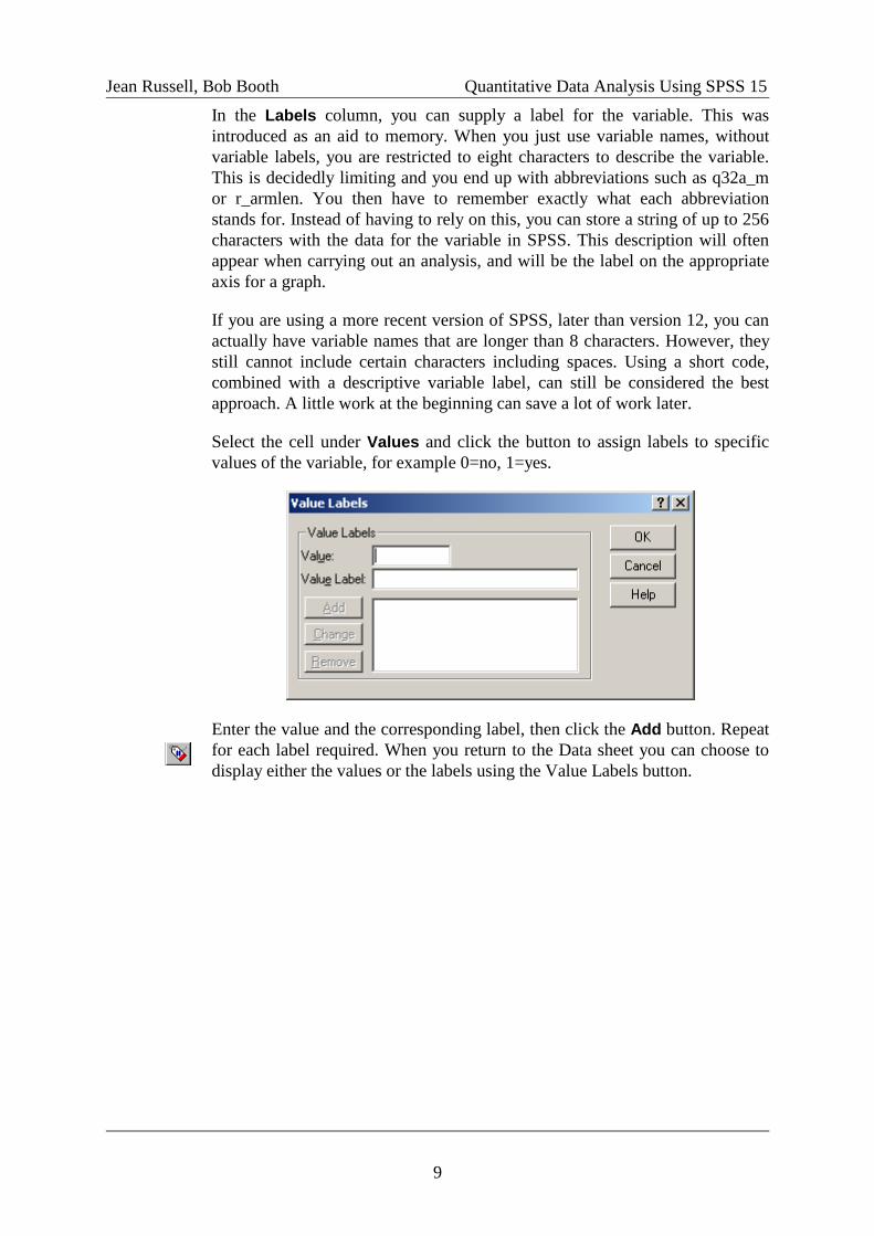
Select the cell under Values and click the button to assign labels to specific

values of the variable, for example 0=no, 1=yes.

Enter the value and the corresponding label, then click the Add button. Repeat

for each label required. When you return to the Data sheet you can choose to

display either the values or the labels using the Value Labels button.


10

You can define how SPSS handles missing data by selecting the cell in the

Missing column, then clicking the button to get the following dialog box.

For a variety of reasons you may not always know the value for a specific case

of a variable. Test results may go missing or off the measurable scale. A

variable may not relate to that case e.g. asking whether a man has had a

hysterectomy. A respondent may refuse to provide the information. SPSS has a

system to deal with missing values for numeric variables, which it uses if a cell

is left blank. This value is represented by the . character. This case would be

dropped from any technique that uses that variable. It is possible to use this

solely for your missing values, but as you get missing ones for different

reasons you may want to distinguish as to why a value is missing. To do so

you need to tell SPSS which values are to be treated as missing. It is also

useful to have value labels for these variables.

There is a variety of missing value conventions. Clearly, the values assigned to

missing codes must be distinct from the values that are likely to occur if you

have a genuine response. One convention used is listed below:

If the variable is categorical (either nominal or ordinal) with a few

categories (5 or less), then the first missing code is normally assigned to 9.

If there is more than one type of missing code, 8 and 7 are used.

If a variable can only take positive numbers then –1 is used as the first

missing code with –2, -3 etc used for further codes.

Otherwise a large negative number is commonly used. It starts with

–999.99, then –888.88 and –777.77 are used for further codes. However,

could equally well choose different numbers.

Entering Data

Once you have defined all your variables you can proceed to type in your data,

as you would a spreadsheet. Place the cursor in the cell where you want to

enter data, then type the value you want and press the Enter key. This will

place the value in the cell and move down to the cell below. You can also

move from cell to cell using the arrow keys, the Tab key, or the mouse.


11

3.2 Saving and Loading SPSS Data

Once you have entered all your data into SPSS you should save it into a data

file. Ideally you should save your data many times before this, say after

defining your variables, then after inputting data for several units, and so on

until your data is complete.

To save your data file either select Save from the File menu, or click on the

usual Save button. You will see a typical Windows Save dialog.

From here you can specify the name for your data file, and use the Save in

field to specify the drive and folder in which to save the file. You can

even use the New Folder button to create a new folder in which to save

your data file.

SPSS data files are usually saved with the extension .sav, but in the Save as

type field you can see some other formats for SPSS data. Data can be saved in

text files with the extension .txt or .dat, or as Excel data with the extension

.xls. You can also save data in other, less common, formats.

When you return to SPSS you can load existing SPSS data files using Open

from the File menu, or by using the usual Open button from the Toolbar. All

the data files ending in .sav will be available, and you can load any data file by

selecting it, then clicking the Open button. In addition you can load data from

other applications, as described in the following sections.


12

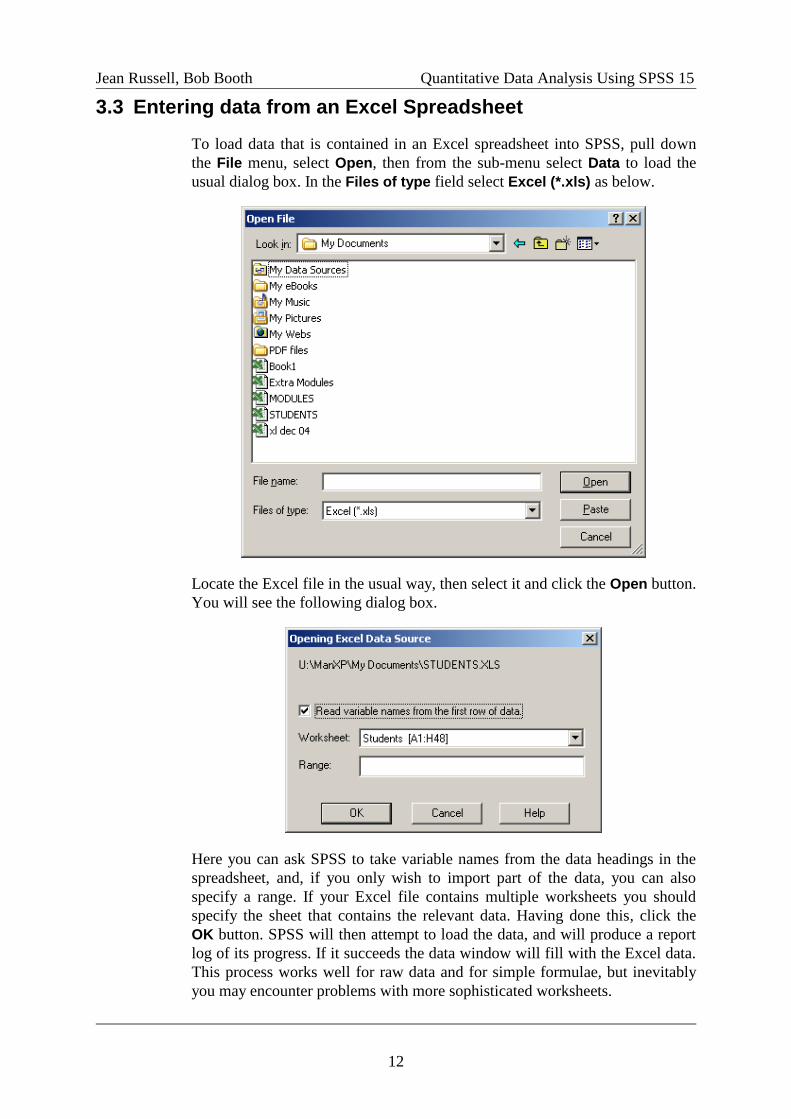
3.3 Entering data from an Excel Spreadsheet

To load data that is contained in an Excel spreadsheet into SPSS, pull down

the File menu, select Open, then from the sub-menu select Data to load the

usual dialog box. In the Files of type field select Excel (*.xls) as below.

Locate the Excel file in the usual way, then select it and click the Open button.

You will see the following dialog box.

Here you can ask SPSS to take variable names from the data headings in the

spreadsheet, and, if you only wish to import part of the data, you can also

specify a range. If your Excel file contains multiple worksheets you should

specify the sheet that contains the relevant data. Having done this, click the

OK button. SPSS will then attempt to load the data, and will produce a report

log of its progress. If it succeeds the data window will fill with the Excel data.

This process works well for raw data and for simple formulae, but inevitably

you may encounter problems with more sophisticated worksheets.


13

3.4 Importing Data from a Text File

Importing data from a text file is more complex than importing it from Excel,

because text files can be much more varied in their data structure. To load a

text file pull down the File menu, but then select Read Text Data. This will

produce an ordinary looking dialog box as below.

Select the data file as usual, then click on the Open button to start a Text

Import Wizard, which will ask you a series of questions about the data before

importing it.

The questions are mostly straightforward, although you might need several

attempts to successfully import your first text file. Once you have answered the

questions on the first screen, select the Next button to proceed to more

questions. It is worth mentioning that screen five displays your variables,

allows you to select each one, and then defines properties for that variable. On

the last screen, screen six, the Finish button becomes available. Click this to

load the data into your data screen. The process may seem daunting, but it

works very well so don't be afraid to try it.


14

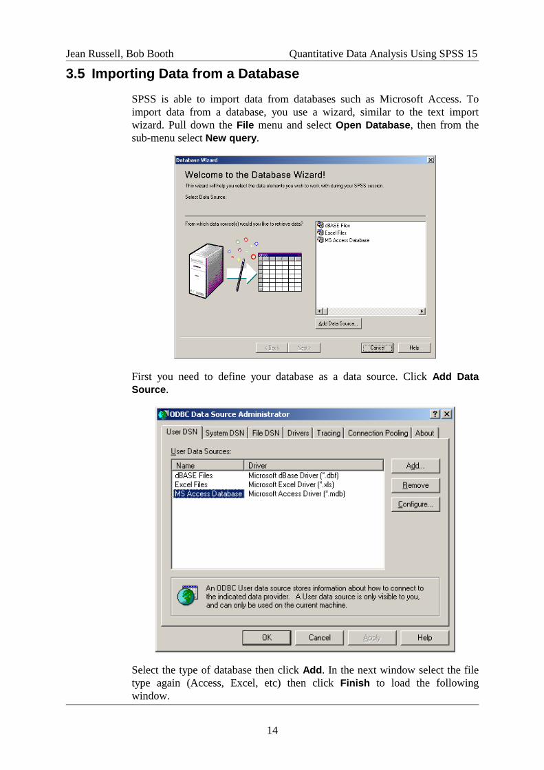
3.5 Importing Data from a Database

SPSS is able to import data from databases such as Microsoft Access. To

import data from a database, you use a wizard, similar to the text import

wizard. Pull down the File menu and select Open Database, then from the

sub-menu select New query.

First you need to define your database as a data source. Click Add Data

Source.

Select the type of database then click Add. In the next window select the file

type again (Access, Excel, etc) then click Finish to load the following

window.


15

Give the database a meaningful name in the Data Source Name box, then

click the Select button to produce a File Open dialog box in which you can

specify the file. Click OK three times to return to the original wizard. Your

new data source will appear in the list, select it then click Next.

The second screen will list the tables and queries from your database. To

import any table or query, drag it from the left window to the right. When you

have done this click the Next button.

In the third screen, specify the relationships between imported tables by

dragging links from one table field to another.

In the fourth screen, specify limits on the imported data fields by building

criteria.

In the fifth screen, specify variable names for all the imported fields.

The sixth screen shows the syntax for the operation. Click the Finish button to

import your data.


16

4. Transforming Variables

SPSS allows you to perform a vast range of calculations on your variables,

including mathematical formulae, logical calculations, occurrence rates,

standard string edits and string to number conversions. These are all available

from the Transform menu, and you can find details on their usage in the SPSS

Help system.

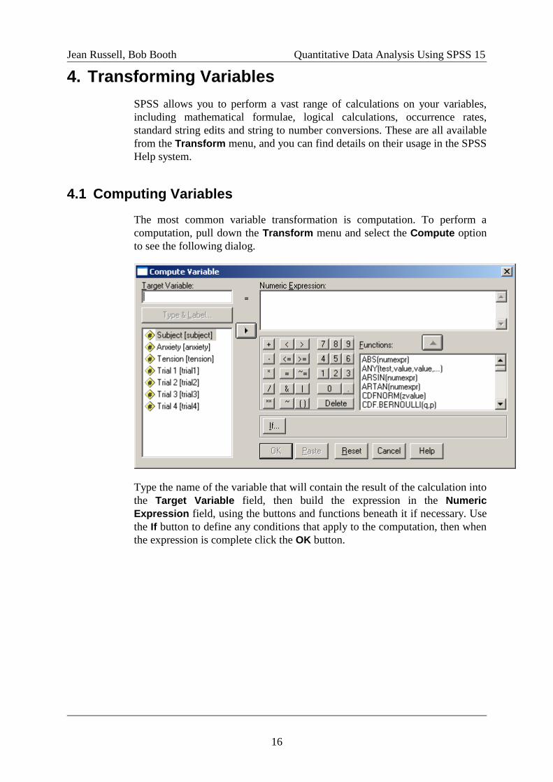
4.1 Computing Variables

The most common variable transformation is computation. To perform a

computation, pull down the Transform menu and select the Compute option

to see the following dialog.

Type the name of the variable that will contain the result of the calculation into

the Target Variable field, then build the expression in the Numeric

Expression field, using the buttons and functions beneath it if necessary. Use

the If button to define any conditions that apply to the computation, then when

the expression is complete click the OK button.


17

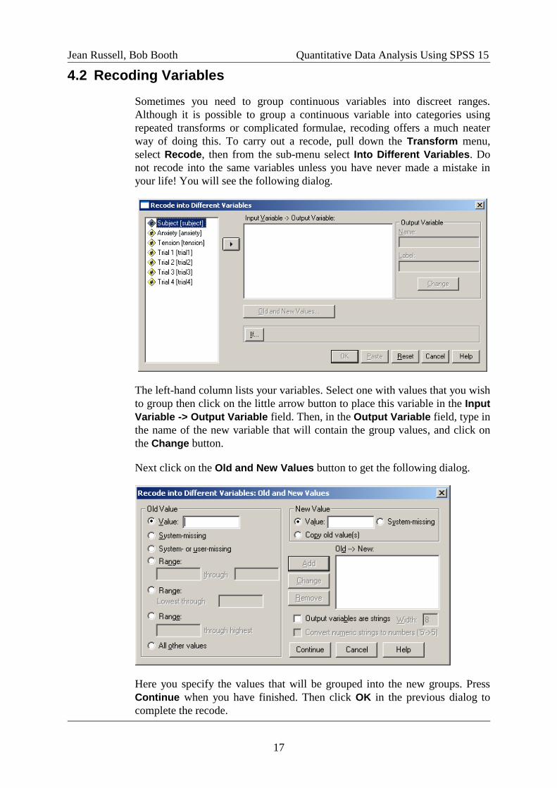
4.2 Recoding Variables

Sometimes you need to group continuous variables into discreet ranges.

Although it is possible to group a continuous variable into categories using

repeated transforms or complicated formulae, recoding offers a much neater

way of doing this. To carry out a recode, pull down the Transform menu,

select Recode, then from the sub-menu select Into Different Variables. Do

not recode into the same variables unless you have never made a mistake in

your life! You will see the following dialog.

The left-hand column lists your variables. Select one with values that you wish

to group then click on the little arrow button to place this variable in the Input

Variable -> Output Variable field. Then, in the Output Variable field, type in

the name of the new variable that will contain the group values, and click on

the Change button.

Next click on the Old and New Values button to get the following dialog.

Here you specify the values that will be grouped into the new groups. Press

Continue when you have finished. Then click OK in the previous dialog to

complete the recode.


18

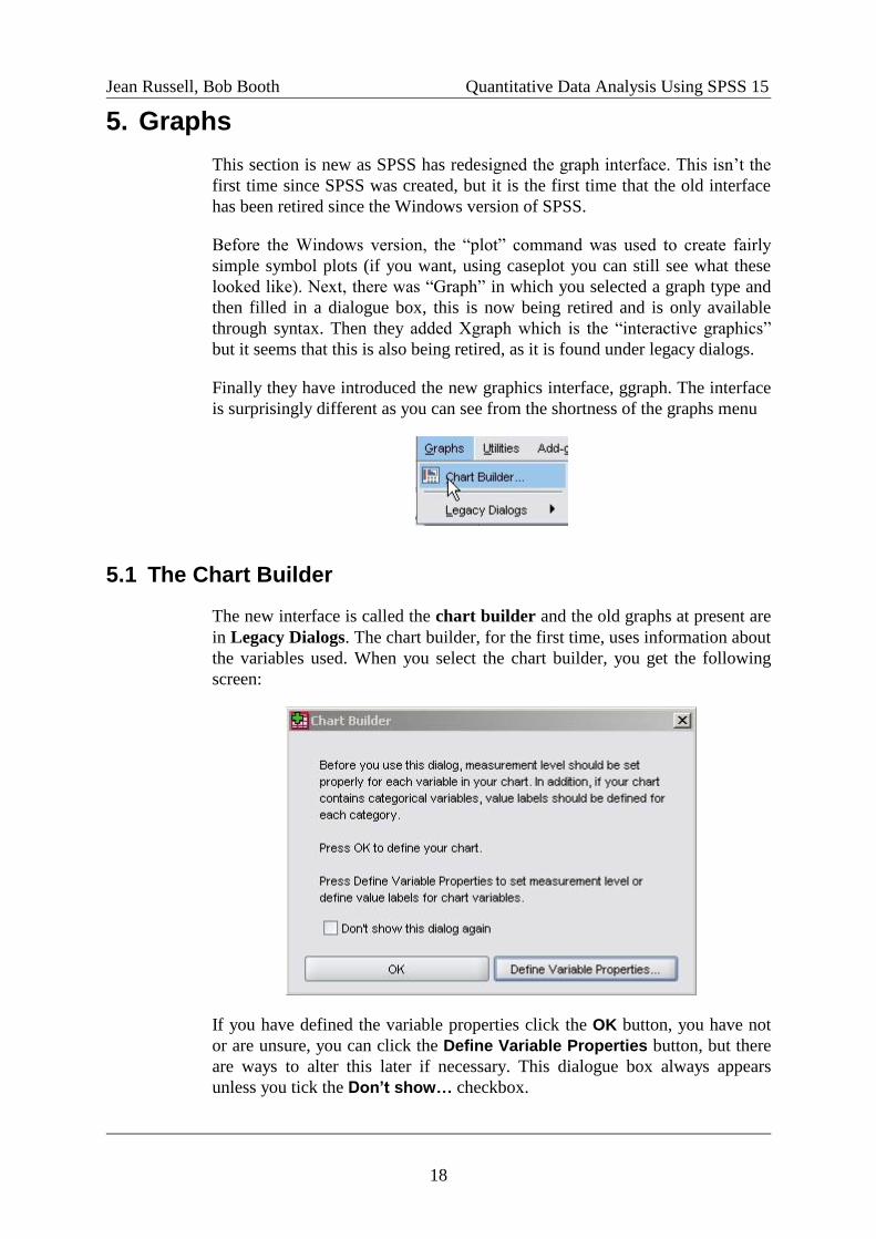
5. Graphs

This section is new as SPSS has redesigned the graph interface. This isn’t the

first time since SPSS was created, but it is the first time that the old interface

has been retired since the Windows version of SPSS.

Before the Windows version, the “plot” command was used to create fairly

simple symbol plots (if you want, using caseplot you can still see what these

looked like). Next, there was “Graph” in which you selected a graph type and

then filled in a dialogue box, this is now being retired and is only available

through syntax. Then they added Xgraph which is the “interactive graphics”

but it seems that this is also being retired, as it is found under legacy dialogs.

Finally they have introduced the new graphics interface, ggraph. The interface

is surprisingly different as you can see from the shortness of the graphs menu

5.1 The Chart Builder

The new interface is called the chart builder and the old graphs at present are

in Legacy Dialogs. The chart builder, for the first time, uses information about

the variables used. When you select the chart builder, you get the following

screen:

If you have defined the variable properties click the OK button, you have not

or are unsure, you can click the Define Variable Properties button, but there

are ways to alter this later if necessary. This dialogue box always appears

unless you tick the Don’t show… checkbox.


19

You will see the Chart Builder dialogue box. Initially, there will be no graph

displayed in the Chart preview area.

The Chart Builder works by drag and drop. Drag a chart type from the

Gallery into the Chart preview area. If your preferred chart type is not

available, you can add new chart type

to the Gallery using the Basic

Elements tab.

When you drag a chart type into the

Chart preview area, the Element

Properties dialogue box will appear.

For the time being, you can ignore this.


20

The Chart preview area in the original dialog box will display your selected

chart type. It will contain blank fields in which you can specify variables.

You can now build your chart by dragging variables from the Variables box

into the element fields indicated by blue dotted lines in the Chart preview

area. The element fields vary according to which chart you are drawing. In the

pie chart they are called Angle Variable and Slice by.

You can change the properties of these elements using the Element

Properties dialogue box, which appeared when you selected a chart type.

Once you have the graph in the form you require, click the OK button to create

the graph in your output.

5.2 Chart Editor

Your graph will almost certainly not be perfect, so you will need to adjust it.

To do that, double-click the graph to view it in the Chart Editor window.

Use the menus to change or add detail to the graph. Most options will use

Element Properties dialogue boxes similar to the one used in creating the

graph. You should experiment with the system and find out what it can do. It is

a fairly basic graphing package, however, so if you need to produce a very

complex or precise graph, you will need to use different software.


21

6. Statistical Techniques

If you are using SPSS you will want to carry out some statistics. The Analyze

menu contains many categories. Each of these leads to sub-menus, which have

several options. In addition, some of these options can carry out a variety of

tests, and there are more time series analyses under the Graphs menu.

6.1 SPSS Statistics Overview

Performing analyses in SPSS is similar to creating graphs; any selection will

present you with a complex dialog box that offers you more control over the

analysis performed. Using linear regression as an example you would see:

The variables are listed on the left-hand side, and you use the small arrow

buttons to place a selected variable into an appropriate field. Again there are

buttons along the bottom of the dialog box that let you define precisely the

type of results you wish to produce.

Once you have defined the analysis click the OK button to carry out the tests

and send the results to the Output window. The results of a general linear

analysis are shown on the next page.


22

A single analysis dialog may produce many tables of statistics. Again, the

more you understand your data the more you can produce meaningful and

useful results. The following sections outline some of the basic analyses

available.

6.2 Frequencies

Use for: Straightforward description of a variable. The options

chosen differ whether one is dealing with continuous or

categorical variables.

Limitations: Tables need turning off for variables with a wide range of

responses.

See: Field p 70-71

Frequencies is the technique used to get a basic description of the data. It will

not only produce a frequency count, but will also calculate a wide range of

statistics, and produce bar charts and histograms. To calculate frequencies, pull

down the Analyze menu and select Descriptive Statistics, then select

Frequencies from the sub-menu. This will bring up the following dialog box:


23

Select a variable to test then use the little arrow button to move this variable

into the Variables field. Use the Statistics, Charts, or Format buttons to

define the required outcome, then click the OK button to perform the test.

6.3 Crosstabs

Use for: Exploring the relationship of two categorical variables.

Limitations: To use the normal chi-squared value you need to have

expected values of greater than five. This caution is

conservative and can be got around by using the exact

statistics. Tables with more than 25 cells are clumsy and

difficult to interpret.

See: Field p 681-694

Crosstabs is the technique used in SPSS to produce cross tabulation of two

variables. As this technique treats the values as categories, it is only sensible to

use this with categorical data. To perform Crosstabs pull down the Analyze

menu, choose Descriptive Statistics, then select Crosstabs. This will bring

up the following dialog box.

You can choose various tests to apply by clicking the Statistics button. Here

you will find the Two-way Pearson Chi-square test. This is the usual Chi-

square test; the one-way Chi-square test, which appears under Nonparametric

tests, is rarely used.

To avoid getting only cell counts in your table, click on the Cells button to get

the following dialog box. Here you can specify the type of results that you

wish to have displayed in the cells.


24

Click Continue to return to the original dialog, then click OK to perform the

Crosstabs analysis.

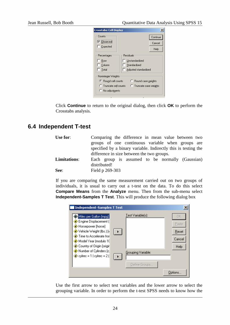
6.4 Independent T-test

Use for: Comparing the difference in mean value between two

groups of one continuous variable when groups are

specified by a binary variable. Indirectly this is testing the

difference in size between the two groups.

Limitations: Each group is assumed to be normally (Gaussian)

distributed!


If you are comparing the same measurement carried out on two groups of

individuals, it is usual to carry out a t-test on the data. To do this select

Compare Means from the Analyze menu. Then from the sub-menu select

Independent-Samples T Test. This will produce the following dialog box

Use the first arrow to select test variables and the lower arrow to select the

grouping variable. In order to perform the t-test SPSS needs to know how the


25

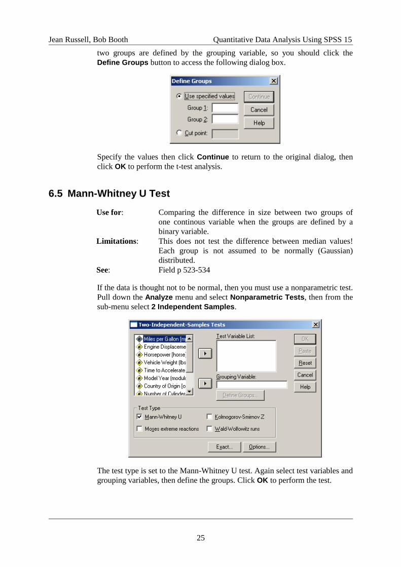
two groups are defined by the grouping variable, so you should click the

Define Groups button to access the following dialog box.

Specify the values then click Continue to return to the original dialog, then

click OK to perform the t-test analysis.

6.5 Mann-Whitney U Test

Use for: Comparing the difference in size between two groups of

one continous variable when the groups are defined by a

binary variable.

Limitations: This does not test the difference between median values!

Each group is not assumed to be normally (Gaussian)

distributed.


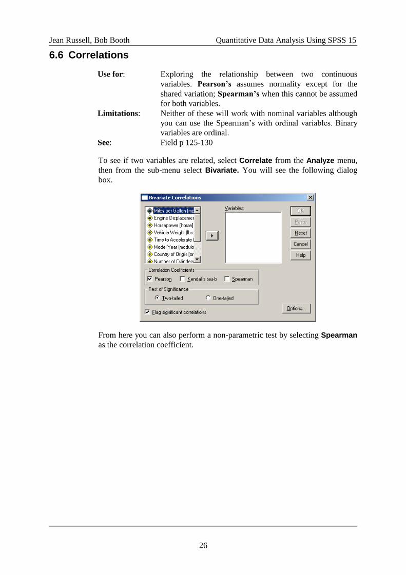
If the data is thought not to be normal, then you must use a nonparametric test.

Pull down the Analyze menu and select Nonparametric Tests, then from the

sub-menu select 2 Independent Samples.

The test type is set to the Mann-Whitney U test. Again select test variables and

grouping variables, then define the groups. Click OK to perform the test.


26

6.6 Correlations

Use for: Exploring the relationship between two continuous

variables. Pearson’s assumes normality except for the

shared variation; Spearman’s when this cannot be assumed

for both variables.

Limitations: Neither of these will work with nominal variables although

you can use the Spearman’s with ordinal variables. Binary

variables are ordinal.


To see if two variables are related, select Correlate from the Analyze menu,

then from the sub-menu select Bivariate. You will see the following dialog

box.

From here you can also perform a non-parametric test by selecting Spearman

as the correlation coefficient.


27

7. Advanced Analyses

7.1 One way ANOVA

Use for: Detecting the difference in mean values of different groups

where there is more than two distinct groups.

Limitations: It is assumed that the populations are normally distributed

and have equal variance. It also assumes that the samples

are independent of each other, which means that each

sample is from a completely separate set of units.

See: Field Chapter 8 pages 309 to362

This is an extension of the T-test for when there are more than two

independent groups. It is possible to compare all pairs separately afterwards

with multiple comparison tests that are less conservative than doing a

Bonferroni correction after doing multiple T-Tests.

From the Analyze menu select Compare Means and then One-way ANOVA.

You will see the following dialog box:

In the Dependent List section, specify the variable that you are interested in

the means of. You may have more than one continuous variable in the

dependent list; SPSS will do a separate ANOVA for each continuous variable

you put in the dependent list. In the Factor box specify the categorical variable

that defines the groups that you want to compare.

To compare pairs of groups, click on Post Hoc button to bring up the

following dialog box.


28

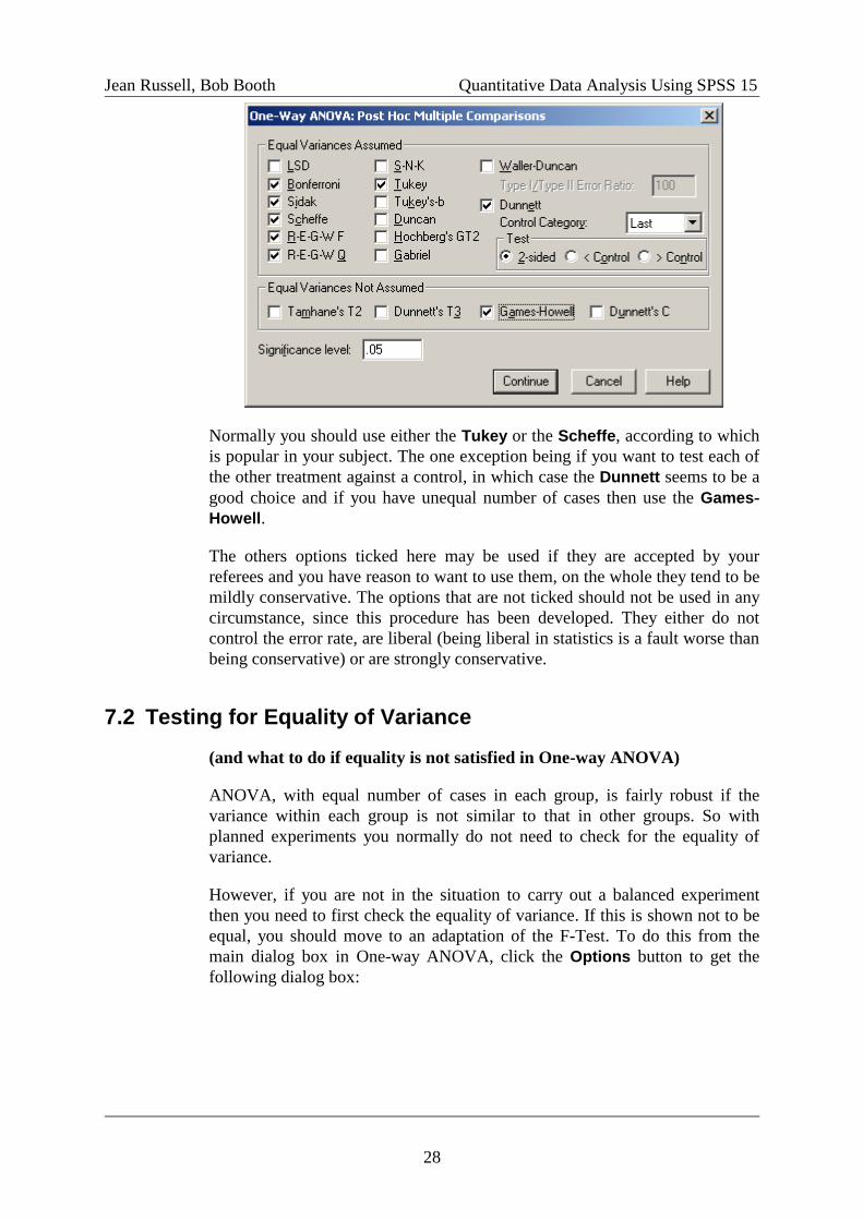
Normally you should use either the Tukey or the Scheffe, according to which

is popular in your subject. The one exception being if you want to test each of

the other treatment against a control, in which case the Dunnett seems to be a

good choice and if you have unequal number of cases then use the Games-

Howell.

The others options ticked here may be used if they are accepted by your

referees and you have reason to want to use them, on the whole they tend to be

mildly conservative. The options that are not ticked should not be used in any

circumstance, since this procedure has been developed. They either do not

control the error rate, are liberal (being liberal in statistics is a fault worse than

being conservative) or are strongly conservative.

7.2 Testing for Equality of Variance

(and what to do if equality is not satisfied in One-way ANOVA)

ANOVA, with equal number of cases in each group, is fairly robust if the

variance within each group is not similar to that in other groups. So with

planned experiments you normally do not need to check for the equality of

variance.

However, if you are not in the situation to carry out a balanced experiment

then you need to first check the equality of variance. If this is shown not to be

equal, you should move to an adaptation of the F-Test. To do this from the

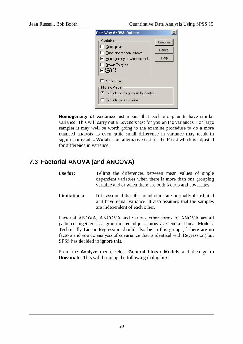
main dialog box in One-way ANOVA, click the Options button to get the

following dialog box:


29

Homogeneity of variance just means that each group units have similar

variance. This will carry out a Levene’s test for you on the variances. For large

samples it may well be worth going to the examine procedure to do a more

nuanced analysis as even quite small difference in variance may result in

significant results. Welch is an alternative test for the F-test which is adjusted

for difference in variance.

7.3 Factorial ANOVA (and ANCOVA)

Use for: Telling the differences between mean values of single

dependent variables when there is more than one grouping

variable and or when there are both factors and covariates.

Limitations: It is assumed that the populations are normally distributed

and have equal variance. It also assumes that the samples

are independent of each other.

Factorial ANOVA, ANCOVA and various other forms of ANOVA are all

gathered together as a group of techniques know as General Linear Models.

Technically Linear Regression should also be in this group (if there are no

factors and you do analysis of covariance that is identical with Regression) but

SPSS has decided to ignore this.

From the Analyze menu, select General Linear Models and then go to

Univariate. This will bring up the following dialog box:


30

In the Dependent Variable section, you should put the continuous outcome

variable that you are interested in. In the Fixed Factors(s) section, specify the

explanatory factors which have had fixed or determined levels, these would

include things like gender and college. Random Factor(s) are where the

selection of levels is a feature of the sampling that has taken place. Example of

a random factor may be country of origin of students entering a University.

Some levels like the UK will come up year after year, but it is unlikely that

every year there would be students from Tonga. So in a sense the countries that

turn up are a result of a random process. Normally, although we are interested

in removing the variance due to a Random Factor, we are not interested in

estimating its effect too precisely. In the Covariate(s) section, we would place

continuous explanatory variables.

Click the Model button to see the following dialog box:


31

With simple ANOVAs like the present one, you can normally go for the

Full factorial model. With complex ones (i.e. with three or more factors and

covariates) it is a good idea to do a custom model, such as the main effects

(factors and covariates) and their two-way interactions. Three-way interactions

and above are notoriously difficult to handle. It is normally a good idea to keep

Sum of Squares set as Type III . On a few occasions a change to Type IV may

be sensible. Types I and II are the same as Type III where you are carrying out a

fully designed study, otherwise they cause problems with interpretation.

The Contrasts button is beyond the scope of this text. If you want to access

the full power of ANOVA then you really do need to get to grips with

contrasts. I suggest that you read section 8.2.10 Planned Contrasts from Field

p 325.

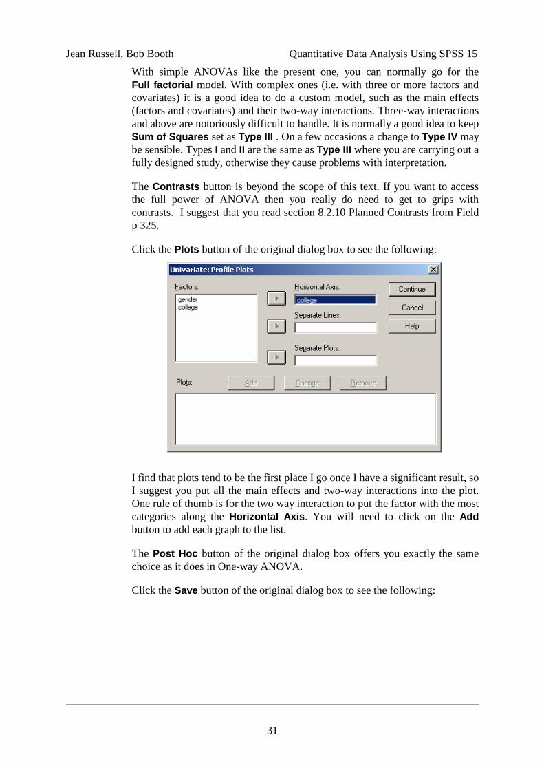
Click the Plots button of the original dialog box to see the following:

I find that plots tend to be the first place I go once I have a significant result, so

I suggest you put all the main effects and two-way interactions into the plot.

One rule of thumb is for the two way interaction to put the factor with the most

categories along the Horizontal Axis. You will need to click on the Add

button to add each graph to the list.

The Post Hoc button of the original dialog box offers you exactly the same

choice as it does in One-way ANOVA.

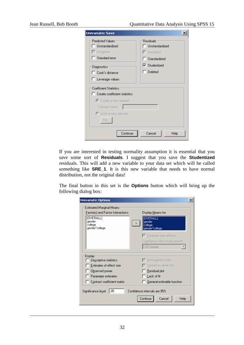
Click the Save button of the original dialog box to see the following:


32

If you are interested in testing normality assumption it is essential that you

save some sort of Residuals. I suggest that you save the Studentized

residuals. This will add a new variable to your data set which will be called

something like SRE_1. It is this new variable that needs to have normal

distribution, not the original data!

The final button in this set is the Options button which will bring up the

following dialog box:


33

I suggest you specify all the factors and factor interactions in the Display

Means for: box as you do not know which you will be interested in, until you

have the ANOVA table in the output. It is also a good idea to tick the

Homogeneity tests and Spread vs. level plot.

When you have worked through all these dialog boxes, click the Ok button.

For Further information: Field chapters 10 and 9 (yes in that order).

Chapter 10 is pp 389-426, chapter 9 pp 363-388

7.4 Checking that the residuals are normally distributed

If you have followed the previous instructions you will have a new variable

called something like SRE_1 added to your data set. As I have said earlier: it

is this variable that needs to be normally distributed. The preferred method by

most statisticians is to use a normal probability plot. To do this, click the

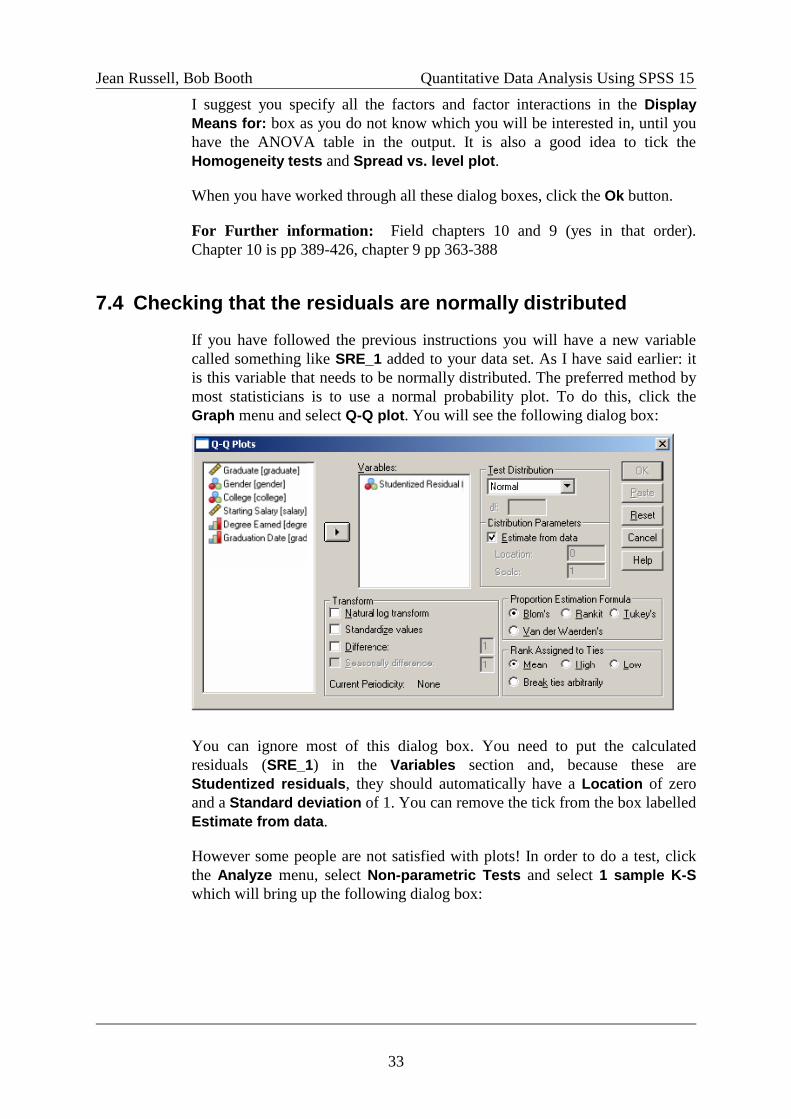
Graph menu and select Q-Q plot. You will see the following dialog box:

You can ignore most of this dialog box. You need to put the calculated

residuals (SRE_1) in the Variables section and, because these are

Studentized residuals, they should automatically have a Location of zero

and a Standard deviation of 1. You can remove the tick from the box labelled

Estimate from data.

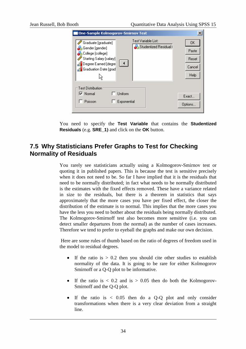
However some people are not satisfied with plots! In order to do a test, click

the Analyze menu, select Non-parametric Tests and select 1 sample K-S

which will bring up the following dialog box:


34

You need to specify the Test Variable that contains the Studentized

Residuals (e.g. SRE_1) and click on the OK button.

7.5 Why Statisticians Prefer Graphs to Test for Checking

Normality of Residuals

You rarely see statisticians actually using a Kolmogorov-Smirnov test or

quoting it in published papers. This is because the test is sensitive precisely

when it does not need to be. So far I have implied that it is the residuals that

need to be normally distributed; in fact what needs to be normally distributed

is the estimates with the fixed effects removed. These have a variance related

in size to the residuals, but there is a theorem in statistics that says

approximately that the more cases you have per fixed effect, the closer the

distribution of the estimate is to normal. This implies that the more cases you

have the less you need to bother about the residuals being normally distributed.

The Kolmogorov-Smirnoff test also becomes more sensitive (i.e. you can

detect smaller departures from the normal) as the number of cases increases.

Therefore we tend to prefer to eyeball the graphs and make our own decision.

Here are some rules of thumb based on the ratio of degrees of freedom used in

the model to residual degrees.

If the ratio is > 0.2 then you should cite other studies to establish

normality of the data. It is going to be rare for either Kolmogorov

Smirnoff or a Q-Q plot to be informative.

If the ratio is < 0.2 and is > 0.05 then do both the Kolmogorov-

Smirnoff and the Q-Q plot.

If the ratio is < 0.05 then do a Q-Q plot and only consider

transformations when there is a very clear deviation from a straight

line.


35

7.6 Linear Regression

Use for: Sorting out relationships between a continuous dependent

variable and continuous (or binary) explanatory variables.

Limitations: It is assumed that once the model is fitted, the residuals are

normally distributed from a single normal distribution. It

does not handle categorical variables that have more than

two categories at all well; indeed the only way to deal

correctly with non-binary categorical variables is to create

dummy variables and use those in the analysis. It is also

assumed that none of the explanatory variables

(independent) are highly correlated with each other.

Another rule of thumb is you need at least five cases for

each explanatory variable and preferably twenty.

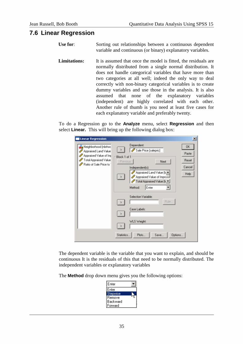
To do a Regression go to the Analyze menu, select Regression and then

select Linear. This will bring up the following dialog box:

The dependent variable is the variable that you want to explain, and should be

continuous It is the residuals of this that need to be normally distributed. The

independent variables or explanatory variables

The Method drop down menu gives you the following options:


36

If you know the model you want to fit then select Enter. There are three

model selection techniques: Stepwise, Backward and Forward. Forward

method starts with no terms (explanatory variables) in the model and at each

step adds the most significant term until there are no more significant terms.

Backward method starts with all terms in the model then deletes the least

significant term until there are only significant terms in the model. Stepwise

checks both the possibility of putting a term in or removing a term and chooses

the best at each step. That leaves Remove which is used on the second or third

step to remove already entered terms to calculate the significance between the

model with them in or with them removed.

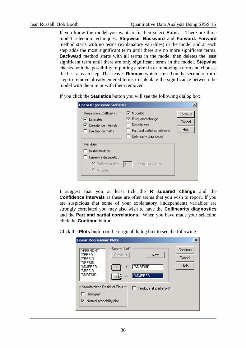
If you click the Statistics button you will see the following dialog box:

I suggest that you at least tick the R squared change and the

Confidence intervals as these are often terms that you wish to report. If you

are suspicious that some of your explanatory (independent) variables are

strongly correlated you may also wish to have the Collinearity diagnostics

and the Part and partial correlations. When you have made your selection

click the Continue button.

Click the Plots button or the original dialog box to see the following:


37

I suggest that you tick the box labelled Normal probability plot at least. For a

scatterplot a useful plot would be the Studentised Deleted Residual SDRESID

against the Adjusted Predictor ADJPRED. When you have selected your plots

then click the Continue button. The Save and Options buttons are for the

specialist use and a basic user is unlikely to want to change any of their current

settings. So you can now click the Ok button.

For further reading: Field Chapter 5 pp143-217

7.7 Logistic Regression

Use for: Sorting out the relationship between a binary dependent and

categorical or continuous explanatory (independent)

variables.

Limitations: Logistic Regression does not work well when any of the

explanatory variables (independent) are highly correlated

with each other. For logistic regression to give good

estimates you need at least 10 cases of your less frequent

outcome per variable. Also the proportion of cases should

be between 5% and 95% in order to get reliable estimates.

If your data does not conform to these limits then you need

to use a package like Cytel’s LogXact.

Please note, Logistic Regression was a much later addition to SPSS than any

other procedure covered up to now. Although many things will seem very

similar some things will differ markedly.

To do a Logistic Regression, click the Analyze menu, select Regression then

select Binary Logistic. You will see the following dialog box:

Your Dependent variable should be a binary variable. That means that you

can rephrase it as a simple yes/no question and get all the data. In this case it is

whether somebody has passed or not when sitting an exam. In the block you

need to put the appropriate covariates for your analysis, in this example score


38

on a preliminary test, which group they were assigned to and how many weeks

of experience they had. Note that these are both continuous and categorical.

Binary Logistic regression handles both sort of variable but you have to tell the

program which variables are categorical. To do this you press the Categorical

button to bring up the following dialog box.

You need to take the categorical explanatory variables into the Categorical

Covariates box. When you have done this click Continue.

The change contrast in this dialog box is useful when you want to test specific

things. I advise you to either look them up in the manual (an extra CD which

you can get from CiCS for £2) and also read about dummy variables in Field

pg 208 as contrasts are already-calculated dummy variables. A good

introduction to contrasts is found the first chapter of Multivariate Analysis

of Variance and Repeated Measures by D. J. Hand and C.C Taylor,

available through Google books.

Click on Options button to see the following dialog box:

I suggest that you tick the Hosmer-Lemeshow goodness of fit box and

CI for exp(B). The first gives an idea of how good a fit the model is, the

second is the confidence interval of the odds ratio! For some reason SPSS has

stuck with the mathematical formula instead of the commonly used name.

For further reading: see Field Chapter 6 pp 218-268


39

8. Interacting with a Word Document

8.1 Putting Data Tables in Word Documents

To copy an SPSS table into a Word table, select the table in the Output

window and choose Copy from the Edit menu. Then go to Word and use

Paste from the Edit menu.

To copy an SPSS table into Word as simple text, select the table in the Output

window and choose Copy from the Edit menu. Then go to Word and from the

Edit menu use Paste Special then select Unformatted Text.

To copy an SPSS table into Word as an SPSS object, select the table in the

Output window and choose Copy Object from the Edit menu. Then go to

Word and use Paste from the Edit menu.

8.2 Putting Graphs in Word Documents

To paste as a simple picture, select the graph and choose Copy from the Edit

menu. Then go to Word and use Paste from the Edit menu.

To paste as an object select the graph and choose Copy Object from the Edit

menu. Then go to Word and use Paste from the Edit menu. This is not

editable within Word. Interactive graphs can only be pasted as objects.

8.3 Exporting to Web Page and Graphics Files

To do this select Export from the File menu of the Output window. Use the

Export list to specify objects to export. For table only files you can export to

HTML or to plain text.

Use the File Type list to choose HTML for data, or a graphics format for

charts. Charts can be exported as Windows metafile (WMF), Windows bitmap

(BMP), encapsulated PostScript (EPS), JPEG, TIFF, CGM, PNG, or

Macintosh PICT.


40

9. Syntax

You can display the line entry commands required to carry out an analysis or

create a graph. Select Options from the Edit menu, then choose the table

labelled Viewer and check the Display commands in the log box. Once the

log is displayed on screen, any analysis you perform will write the equivalent

line entry commands into the on-screen log.

A text file that contains the commands to carry out an analysis in SPSS is

called a Syntax File. To open one of these go to the File menu, select New,

then select Syntax. This is a straight text file and you type in the relevant

commands. It can be saved to run again later, which you cannot do with a

series of keystrokes.

10. Further Reading

SPSS Books

Discovering Statistics Using SPSS, Andy Field, Sage Publications, ISBN 0-

7619-4452-4

This is a book that is both a statistics text and an SPSS primer. It covers a

large number of techniques (all introduced in this course and more) along with

the background theory of how they work. For those who want to go further, I

have referenced the relevant pages in Field for each statistical technique

covered in this userguide.

SPSS Made Simple, Kinnear & Grey, ISBN 0-8637-7350-8, £12.43 for v 15

A good introduction to SPSS, costing about half the price of a single manual.

It is written by academics in Aberdeen.

SPSS Guide to Data Analysis, Marya Norusis, ISBN 0-13-020399-8. £44.99

More than a manual, it details why and how to use SPSS for analysing your

data. It has become a classic, but costs about twice as much as Kinnear &

Grey. If you want a book from SPSS, this is preferable to a manual.

General Statistics Books

The Cartoon Guide to Statistics, ISBN 0-5062731025, £9.99

A basic introduction to statistical thinking.

How to Lie with Statistics, ISBN 0-393310728, £5.99

This book is a good read, even if the closest you get to statistics is reading

what someone else has done. It goes through the basic ways that research may

be reported to mislead.