DANISH METEOROLOGICAL INSTITUTE ————— SCIENTIFIC REPORT —————

03-14

Long-Term Probabilistic Atmospheric Transport and Deposition Patterns from Nuclear Risk Sites

in Euro-Arctic Region

Alexander Mahura1,2, Alexander Baklanov1, Jens Havskov Sørensen1

1 Danish Meteorological Institute, Copenhagen, Denmark 2 Institute of Northern Environmental Problems, Kola Science Centre, Apatity, Russia

Arctic Risk Project of the Nordic Arctic Research Programme (NARP)

COPENHAGEN 2003

ISSN: 0905-3263 (printed) ISSN: 1399-1949 (online)

ISBN: 87-7478-490-0

1

TABLE OF CONTENTS

SUMMARY ____________________________________________________________________ 2

I. INTRODUCTION _____________________________________________________________ 3

II. SELECTED APPAROACHES __________________________________________________ 4

2.1. NUCLEAR RISK SITES OF INTEREST ______________________________________________ 4

2.2. INPUT METEOROLOGICAL DATA _________________________________________________ 5

2.3. LONG-TERM DISPERSION MODELLING USING DERMA_____________________________ 5

2.4. INDICATORS OF NRS IMPACT BASED ON DISPERSION MODELLING RESULTS _______ 6

III. ASSESSMENT OF ATMOSPHERIC DISPERSION MODELLING RESULTS FROM

NUCLEAR RISK SITES IN EURO-ARCTIC REGION ________________________________ 8

3.1. TIME INTEGRATED AIR CONCENTRATION PATTERNS FOR 137

CS ____________________ 9

3.2. DRY DEPOSITION PATTERNS FOR 137

CS __________________________________________ 11

3.3. WET DEPOSITION PATTERNS FOR 137

CS __________________________________________ 13

3.4. GENERAL STATISTICS AND CORRELATIONS BETWEEN PATTERNS ________________ 15

3.5. INDICATORS OF NRS IMPACT FOR EMERGENCY RESPONSE AND PREPAREDNESS __ 21

3.6. SPECIFIC CASE STUDIES FOR 137

CS,131

I,90

SR, AND 85

KR RELEASES_________________ 24

3.7. ESTIMATION OF POTENTIAL IMPACT AT COPENHAGEN, DENMARK DUE TO

RELEASES AT SELECTED NUCLEAR RISK SITES______________________________________ 33

CONCLUSIONS _______________________________________________________________ 36

RECOMMENDATIONS FOR FUTURE STUDIES __________________________________ 37

ACKNOWLEDGMENTS ________________________________________________________ 39

REFERENCES ________________________________________________________________ 40

ABBREVIATIONS _____________________________________________________________ 42

Scientific Reports ______________________________________________________________ 43

APPENDIX 1 _________________________________________________________________ 47

APPENDIX 2 _________________________________________________________________ 64

2

SUMMARY

The main purpose of the Arctic Risk, NARP multidisciplinary project is to develop a

methodology for complex nuclear risk and vulnerability assessment and to test it by estimation of a

nuclear risk to population in the Nordic countries in case of a severe accident at nuclear risk sites

(NRSs). This report is focused on the testing of the developed methodology (AR-NARP, 2001-2003;

Baklanov et al., 2002b) and probabilistic evaluation of the long-term atmospheric transport and

deposition patterns for radioactive pollutants from selected 16 risk sites in the Euro-Arctic region.

The main questions to be addressed are:

What geographical territories and neighbouring countries are at the highest risk of being

polluted during atmospheric transport and deposition in case of an hypothetical accident at NRS?

What are levels of contamination on local, regional, and large scales due to dry and wet

deposition in case of a hypothetical accident at NRS? To answer these questions, at first, we applied a combination of DMI’s models - 3-D

trajectory, DERMA, and HIRLAM. These models were used to simulate a long-term (during year

of 2002) atmospheric transport, dispersion, and deposition of 137

Cs for a one day hypothetical

release (at rate of 1011

Bq/s). Then, a set of statistical methods (including exploratory and

probability fields analyses) was employed for probabilistic analysis of dispersion modelling results

in order to evaluate variability of annual, seasonal, and monthly NRS possible impact indicators,

such as average and summary time integrated air concentration (TIAC), dry deposition (DD) and

wet deposition (WD) fields.

Among 16 NRSs several groups can be identified based on spatial and temporal variability of

calculated fields: sites located in the maritime, continental, arctic, and intermediate (maritime vs.

continental) areas. For most of NRSs the prevailing atmospheric transport is by westerlies. The

TIAC and DD fields have an elliptical shape compared with more cellular structure of the WD field

which strongly depends on irregularity of the rainfall patterns. Moreover, the WD fields can have

several local maxima remotely situated from the sites. The ranking of potential impact on

Copenhagen, Denmark from selected 16 NRSs of the Euro-Arctic region showed that although for

TIAC and DD the order of such ranking is identical; when additionally a wet deposition is

accounted the ranks can change significantly already on mesoscales. Due to a relative proximity (

500 km) to Copenhagen, the Barsebaeck, block of the German nuclear power plants (NPPs),

Oskarshamn, and Ringhals NPPs represent the risk sites of major concern for the city. Although

several other sites such as the Olkiluoto, Ignalina, Loviisa, and Forshmark plants are located

geographically closer to the city, the block of the British NPPs (> 1000 km) represents the higher

risk of airborne transport potential impact on Copenhagen compared with them.

The results of this study are applicable for: (i) better understanding of general atmospheric

transport patterns in the event of an accidental release at NRS, (ii) improvement of planning in

emergency response to radionuclide releases from the NRS locations, (iii) studies of social and

economical consequences of the NRS impact on population and environment of the neighbouring

countries, (iv) multidisciplinary risk evaluation and vulnerability analysis, (v) probabilistic

assessment of radionuclide regional and long-range transport patterns, and (vi) evaluation of

integrated impact from the long-term releases/ emissions.

The annual, seasonal, and monthly variability of the time integrated air concentration, dry,

and wet deposition fields are stored on CD (enclosed with this report with enlarged figures, if

ordered).

3

I. INTRODUCTION

Many international research projects have realized models and methods describing separate

parts in evaluation of the risk assessment, e.g. the probabilistic safety assessment, long-range

transport and contamination modelling, radioecological sensitivity, dose estimation, etc. However,

methodologies for multidisciplinary studies of nuclear risk assessments and mapping are not well

developed yet (cf. e.g. Baklanov, 2002). As shown in IIASA, 1996, the risk-assessment strategy can

be realised by the following methods: inference from actual events (i.e. using published results from

real events); physical modelling (i.e. using known input and prevalent levels); and theoretical

modelling (i.e. using simulated response to assumed scenarios of releases). Description and results

of these methods with respect to nuclear risk sites are shown by IIASA, 1996; Moberg, 1991;

Bergman et al., 1998; Dahlgaard, 1994; Bergman & Ulvsand, 1994; Amosov et al., 1995;

Rantalainen, 1995.

For probabilistic analysis some authors performed studies based on combination of different

factors and probabilities. Previous research in the Arctic latitudes were based on employing of the

trajectory modelling approach to evaluate potential impact from nuclear plants such as Kola

(Saltbonis, ; Baklanov et al., 2002a) and Bilibino (Mahura et al., 1999). The dispersion modelling

approach was used by Slaper et al., 1994 whom evaluated dispersion of the radioactive plume by a

simple model (based on only meteorological station) in order to estimate risks, health effects, and

countermeasures due to severe accidents at the European NPPs (including the northern latitudes

plants) and a submarine (NATO, 1998). Sinyak, 1995 used some empirical factors to describe the

influences of geography resulting in normalized damage factors for the main European cities.

Andreev et al., 1998; 2000 simulated dispersion and deposition with a Lagrangian particle model

and calculated the frequency of exceedance of certain thresholds for 137

Cs, regarded as a risk

indicator.

The dispersion and deposition models can be successfully used for separate case studies for

typical or worst-case scenarios. They can be used also for probabilistic risk mapping as a more

expensive, but alternative of the trajectory analysis methods discussed for the nuclear risk sites by

Baklanov & Mahura, 2001; Mahura & Baklanov, 2002. Applicability and examples of different

models for accidental release dispersion and deposition simulation on the local and regional scales

in the Arctic were discussed by Baklanov et al., 1994; Thaning & Baklanov, 1997; Baklanov, 2000;

Baklanov et al., 2001; Baklanov & Sørensen, 2001).

The methodology, developed in the bounds of the Arctic Risk project (AR-NARP, 2001-2003)

is a logical continuation, as mentioned by Baklanov et al., 2002b, of several previous studies

realised in the frameworks of international projects. It includes several specific approaches in

optimal strategy of the multidisciplinary methodology. Among these approaches is a combination of

the probabilistic analysis and case studies analysis.

In previous AR-NARP project reports (Baklanov & Mahura, 2001; Mahura & Baklanov,

2002; Baklanov et al., 2002b) we described a methodology of trajectory and dispersion modelling

approaches, methodology results of probabilistic analysis of atmospheric transport pattern and risk

assessment based on trajectory modelling. The main purpose of this report is to test and employ the

developed methodology (e.g. AR-NARP, 2001-2003; Baklanov et al., 2002b) based on a long-term

dispersion modelling approach in order to evaluate temporal and spatial variability of atmospheric

transport and deposition patterns from sixteen nuclear risk sites in the Euro-Arctic region, and use

these patterns for further integration in GIS for risk and vulnerability mapping.

4

II. SELECTED APPAROACHES

2.1. NUCLEAR RISK SITES OF INTEREST

All selected NRSs are located within the area of interest of the “Arctic Risk” Project. These

NRSs are represented mostly by the nuclear power plants (NPPs) in Russia, Lithuania, Germany,

United Kingdom, Finland, Ukraine, and Sweden (see Tab. 2.1.1, Fig. 2.1.1). It should be noted that

the Kola NPP (KNP, Murmansk Region, Russia) has the old type of reactors (VVER-230);

Leningrad (LNP, Leningrad Region, Russia), Chernobyl (CNP, Ukraine), and Ignalina (INP,

Lithuania) NPPs have the most dangerous RBMK-type reactor. Moreover, the Novaya Zemlya

(NZS, Novaya Zemlya Archipelago, and Russia) was considered as the former nuclear weapon test

site and potential site for nuclear waste deposit; and the Roslyakovo shipyard (KNS, Murmansk

Region, Russia) was considered as a risk site with nuclear power ships in operation or waiting to be

decommissioned.

Table 2.1.1. Nuclear risk sites selected for the “Arctic Risk” Project.

# Site Lat,°N Lon,°E Site Names Country

1 KNP 67.75 32.75 Kola NPP Russia

2 LNP 59.90 29.00 Leningrad NPP Russia

3 NZS 72.50 54.50 Novaya Zemlya Test Site Russia

4 INP 55.50 26.00 Ignalina NPP Lithuania

5 BBP 54.50 -3.50°W Block of the British NPPs United Kingdom

6 BGP 53.50 9.00 Block of the German NPPs Germany

7 LRS 60.50 26.50 Loviisa NPP Finland

8 TRS 61.50 21.50 Olkiluoto (TVO) NPP Finland

9 ONP 57.25 16.50 Oskarshamn NPP Sweden

10 RNP 57.75 12.00 Ringhals NPP Sweden

11 BNP 55.75 13.00 Barsebaeck NPP Sweden

12 FNP 60.40 18.25 Forshmark NPP Sweden

13 KRS 51.70 35.70 Kursk NPP Russia

14 SNP 54.80 32.00 Smolensk NPP Russia

15 CNP 51.30 30.25 Chernobyl NPP Ukraine

16 KNS 69.20 33.40 Roslyakovo Shipyard Russia

The Block of the British NPPs (BBP) is represented by a group of the risk sites: the Sellafield

reprocessing plant, Chapelcross (Annan, Dumfriesshire), Calder Hall (Seascale, Cumbria),

Heysham (Heysham, Lancashire), and Hunterston (Ayrshire, Strathclyde) NPPs. The Block of the

German NPPs (BGP) is represented by a group of NPPs: Stade (Stade, Niedersachsen), Kruemmel

(Geesthacht, Schleswig-Holstein), Brunsbuettel (Brunsbuettel, Schleswig-Holstein), Brokdorf

(Brokdorf, Schleswig-Holstein), and Unterweser (Rodenkirchen, Niedersachsen). Although these

NPPs use different reactor types and, hence, could have different risks of accidental releases, the

grouping is relevant for airborne transport studies because all NPPs are located geographically close

to each other and, hence, atmospheric transport patterns will be relatively similar. The further

evaluation of risk levels can be calculated for each NPP separately based on the atmospheric

transport fields and probabilities of accidents for each NPP.

5

Figure 2.1.1. Selected nuclear risk sites of interest.

2.2. INPUT METEOROLOGICAL DATA

In our study, we used two types of the gridded datasets, as input data, for the dispersion

modelling purposes. They are the DMI-HIRLAM (HIgh Resolution Limited Area Model) and

ECMWF (European Centre for Medium-Range Weather Forecast) datasets. The detailed

description of these gridded datasets is given by Baklanov et al. (2002).

The DMI-HIRLAM dataset was used to model atmospheric transport, dispersion, and

deposition only of 137

Cs for 16 NRSs during Fall 2001 - Spring 2003 (and will continue through the

year of 2003 to obtain further the inter-annual variability of calculated parameters and longer

multiyear statistics which is more representative compared with a short-term modelling). The

ECMWF dataset (domain covers nearly the entire Northern Hemisphere, i.e. extends between

12˚N–90˚N vs. 180˚W–180˚E) was used to model atmospheric transport, dispersion, and deposition

for three radionuclides - 137

Cs, 131

I, and 90

Sr – but only from one NRS (Leningrad NPP).

The model runs based on different types of datasets were performed for comparison purposes,

and first of all, to compare the accuracy of the wet deposition patterns. For the specific case studies,

both datasets were used.

2.3. LONG-TERM DISPERSION MODELLING USING DERMA

In this study, we used the Danish Emergency Response Model for Atmosphere (DERMA),

developed by DMI for nuclear emergency preparedness purposes, which is a numerical 3-D

atmospheric model of the Lagrangian type. DERMA was used to simulate a long-term (during year

of 2002) atmospheric transport, dispersion, and deposition of radionuclide from the selected NRSs.

It considered also processes of radioactive decay and removal by precipitation during atmospheric

transport. As input meteorological data, DERMA uses: 1) the Numerical Weather Prediction

(NWP) model data from different operational versions of the HIRLAM or 2) global model of the

European Centre for Medium-Range Weather Forecast (ECMWF) model data. The detailed

6

description of the DERMA model is given by Sørensen, 1998; Sørensen et al., 1998; Baklanov & Sørensen, 2001; Baklanov et al., 2002b and used in this study assumptions by Baklanov et al.,

2002b.It should be repeated again that the following characteristics (for a daily continuous discrete

unit hypothetical release (DUHR) of 137

Cs at NRSs at rate of 1011

Bq/s) were calculated: 1) air

concentration (Bq/m3) in the surface layer; 2) time-integrated air concentration (Bq·h/m

3); 3) dry

and wet deposition (Bq/m2) fields. These fields were recalculated in a gridded domain of a

resolution of 0.5˚ vs. 0.5˚ of latitude vs. longitude, shown in Fig. 2.3.1 (30-89˚N vs. 60˚W-135˚E).

Moreover, these fields are limited during one year by consideration of 5 days of atmospheric

transport of radioactive matter after release ended.

The SGI Origin scalar server was used for DERMA runs and the NEC SX6 supercomputer

system of DMI was used for DMI-HIRLAM modelling computational purposes. All modelled data

were stored on the DMI UniTree mass-storage device as well as recorded on CDs.

Figure 2.3.1. Domain of recalculated dispersion modelling fields.

2.4. INDICATORS OF NRS IMPACT BASED ON DISPERSION MODELLING RESULTS

Two approaches were selected to construct fields for calculated characteristics during the time

period of interest (for instance: month, season, or year). The first type – summary field – is based on

calculating the distribution of the total sum of daily DUHR of radioactivity at NRS during the

period considered, and note that it is a field integrated over this period. This type of field shows the

most probable geographical distribution of radionuclide when the release of radioactivity occurred

during the entire period considered. The second type – average field – is based on calculating the

average value from the summary field. This type of field shows the most probable geographical

distribution of radionuclide when the release of radioactivity occurred during one average day

within the period considered.

In this report we presented only the time integrated air concentration (TIAC), dry deposition

(DD), and wet deposition (WD) patterns from all potential indicators of the NRS impact (shown in

Fig. 2.4.1) on selected geographical regions and territories, and countries of concern (shown in Fig.

2.4.2). The total deposition (TD) fields can be simply calculated by summing of the dry and wet

7

depositions. Only one year (January-December 2002) of calculated fields was used to construct the

NRS impact indicators. For convenience of comparison the temporal variability in characteristic

patterns was underlined by isolines at similar intervals, although every field can be easily

reconstructed with different threshold orders of magnitude than selected. It should be noted that

although these fields were calculated for DUHR, it is possible to recalculate or rescale them for

another accidental release of radioactivity at different magnitude rates. Other assumptions used in

this study are discussed by Baklanov et al., 2002b.

Figure 2.4.1. Indicators of nuclear risk site impact based on dispersion modelling results.

Figure 2.4.2. Geographical regions, territories, and countries selected for the “Arctic Risk”.

INDICATORS OF NRS IMPACT

SUMMARY FIELDS OF

Time Integrated

Air Concentration

Wet

Deposition

Dry

Deposition

Air

Concentration

Total

Deposition

AVERAGE FIELDS OF

Time Integrated

Air Concentration

Air

Concentration

Wet

Deposition

Dry

Deposition

Total

Deposition

8

III. ASSESSMENT OF ATMOSPHERIC DISPERSION MODELLING

RESULTS FROM NUCLEAR RISK SITES IN EURO-ARCTIC REGION

In this chapter, we will focus on evaluation of the long-term dispersion modelling results

(based on modelling of 5 days atmospheric transport after the hypothetical releases completed at the

sites) which are represented as indicators of the NRS impact. Moreover, we will consider several

specific case studies. Using such indicators (based on dispersion modelling results) of the NRS

impact we plan further to employ different dose calculation models as well as the GIS-based risk

and vulnerability analysis for population and environment, first of all, of the Nordic countries.

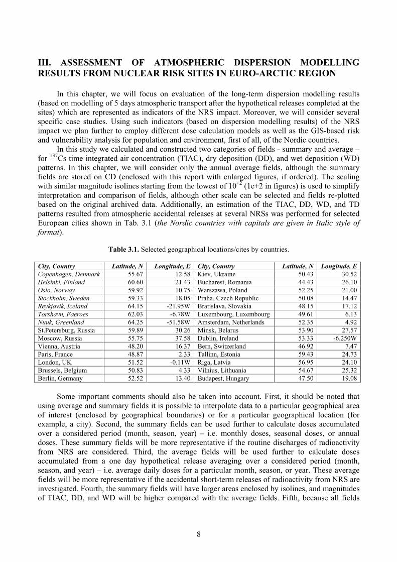
In this study we calculated and constructed two categories of fields - summary and average –

for137

Cs time integrated air concentration (TIAC), dry deposition (DD), and wet deposition (WD)

patterns. In this chapter, we will consider only the annual average fields, although the summary

fields are stored on CD (enclosed with this report with enlarged figures, if ordered). The scaling

with similar magnitude isolines starting from the lowest of 10+2

(1e+2 in figures) is used to simplify

interpretation and comparison of fields, although other scale can be selected and fields re-plotted

based on the original archived data. Additionally, an estimation of the TIAC, DD, WD, and TD

patterns resulted from atmospheric accidental releases at several NRSs was performed for selected

European cities shown in Tab. 3.1 (the Nordic countries with capitals are given in Italic style of

format).

Table 3.1. Selected geographical locations/cites by countries.

City, Country Latitude, N Longitude, E City, Country Latitude, N Longitude, E

Copenhagen, Denmark 55.67 12.58 Kiev, Ukraine 50.43 30.52

Helsinki, Finland 60.60 21.43 Bucharest, Romania 44.43 26.10

Oslo, Norway 59.92 10.75 Warszawa, Poland 52.25 21.00

Stockholm, Sweden 59.33 18.05 Praha, Czech Republic 50.08 14.47

Reykjavik, Iceland 64.15 -21.95W Bratislava, Slovakia 48.15 17.12

Torshavn, Faeroes 62.03 -6.78W Luxembourg, Luxembourg 49.61 6.13

Nuuk, Greenland 64.25 -51.58W Amsterdam, Netherlands 52.35 4.92

St.Petersburg, Russia 59.89 30.26 Minsk, Belarus 53.90 27.57

Moscow, Russia 55.75 37.58 Dublin, Ireland 53.33 -6.250W

Vienna, Austria 48.20 16.37 Bern, Switzerland 46.92 7.47

Paris, France 48.87 2.33 Tallinn, Estonia 59.43 24.73

London, UK 51.52 -0.11W Riga, Latvia 56.95 24.10

Brussels, Belgium 50.83 4.33 Vilnius, Lithuania 54.67 25.32

Berlin, Germany 52.52 13.40 Budapest, Hungary 47.50 19.08

Some important comments should also be taken into account. First, it should be noted that

using average and summary fields it is possible to interpolate data to a particular geographical area

of interest (enclosed by geographical boundaries) or for a particular geographical location (for

example, a city). Second, the summary fields can be used further to calculate doses accumulated

over a considered period (month, season, year) – i.e. monthly doses, seasonal doses, or annual

doses. These summary fields will be more representative if the routine discharges of radioactivity

from NRS are considered. Third, the average fields will be used further to calculate doses

accumulated from a one day hypothetical release averaging over a considered period (month,

season, and year) – i.e. average daily doses for a particular month, season, or year. These average

fields will be more representative if the accidental short-term releases of radioactivity from NRS are

investigated. Fourth, the summary fields will have larger areas enclosed by isolines, and magnitudes

of TIAC, DD, and WD will be higher compared with the average fields. Fifth, because all fields

9

were calculated for the discrete unit hypothetical release (DUHR), it is possible to recalculate or

rescale these fields for other accidental release of radioactivity at different magnitude rates. Sixth, in

calculating atmospheric transport and deposition of radioactivity releases (with a duration of one

day) at NRSs, we limited our calculation to 5 days after the release was completed at the site. As

uncertainties in modelling of atmospheric transport after 5 days became too great, for the calculated

fields of one-day releases we did not apply any loss processes after that 5 day term. It might be that

after this term the trajectories still did not leave the model grid domain and following the mass

conservation law these trajectories will provide additional contributions into concentration and

deposition fields. But, we assume, that mostly trajectories will leave the selected domain with

regions of interest in our study (shown in Fig. 2.3.1) and contributions at boundaries of the

calculated fields will be significantly smaller, is the average fields are considered. Moreover, once

material was deposited on the surface, the radioactive decay was not considered, although it should

be accounted for further risk and vulnerability analyses.

3.1. TIME INTEGRATED AIR CONCENTRATION PATTERNS FOR 137

CS

The time integrated air concentration (TIAC) of a radionuclide is input data to calculate doses

due to inhalation. It is an air concentration of radionuclides accumulated during a selected time

interval. Therefore, for example, for a particular month, the average monthly field might be used to

calculate an average dose due to inhalation at any selected geographical location at any given day of

a particular month. The summary monthly field might be used to calculate the monthly dose due to

inhalation at any selected geographical location.

Let us mention some common peculiarities. First, the time integrated air concentration fields

have a distribution type of isolines around the site, which is closer to elliptical than circular. The

shape of these fields, in some way, reflects the presence of dominating airflow patterns throughout

the year. These airflow patterns could be also obtained from the results of trajectory modelling,

cluster analysis, and probability fields analysis of 5-day trajectories given by Mahura & Baklanov,

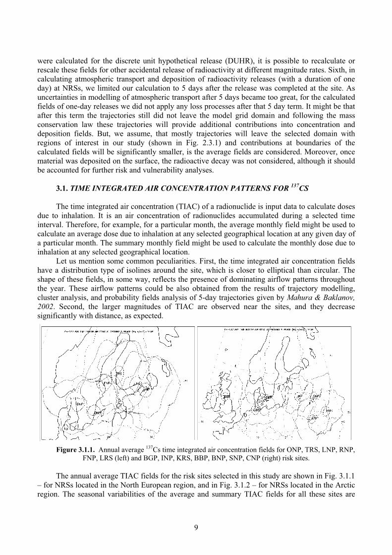
2002. Second, the larger magnitudes of TIAC are observed near the sites, and they decrease

significantly with distance, as expected.

Figure 3.1.1. Annual average 137Cs time integrated air concentration fields for ONP, TRS, LNP, RNP,

FNP, LRS (left) and BGP, INP, KRS, BBP, BNP, SNP, CNP (right) risk sites.

The annual average TIAC fields for the risk sites selected in this study are shown in Fig. 3.1.1

– for NRSs located in the North European region, and in Fig. 3.1.2 – for NRSs located in the Arctic

region. The seasonal variabilities of the average and summary TIAC fields for all these sites are

10

shown in Appendixes 1 and 2, and monthly variability - on CD (enclosed with this report with

enlarged figures, if ordered). For simplicity of interpretation and comparison two isolines of 1e+2

(or 10+2

) and 1e+3 (10+3

) Bq·h/m3were plotted on figures.

Figure 3.1.2. Annual average 137Cs time integrated air concentration fields for KNS, KNP, and NZS

risk sites.

On an annual scale, the highest TIAC ( 1e+3 Bq·h/m3) are within a first few hundred

kilometres around all NRSs. The isolines of 1e+2 Bq·h/m3

for both Arctic NRSs - NZS and KNS -

are more extended in the southern sector from the sites compared to northern sector. For NZS this

isoline passes over un-populated areas compared with the KNS and KNP sites. The populated

territories of the Kola Peninsula and Karelia as well as northern territories of Norway and Finland

are enclosed by isoline of 1e+2 Bq·h/m3, and they remain more affected by potential accidental

releases compared with other territories. Note when only trajectories for the NZS site (see analysis

of trajectory modelling results by Mahura & Baklanov; 2001) were used to construct the airflow

probability fields than the total area of the territories situated under the potential impact from this

site was higher compared with other sites. The dispersion approach gave another picture because of

including effects of stronger dispersion for the strong wind situations in the Arctic latitudes.

Table 3.1.1. Annual average 137Cs time integrated air concentration at selected European cities

resulted from the hypothetical release at the Leningrad NPP.

City, Country

Dist to

LNP,

km

TIAC,

Bq·h/m3City, Country

Dist to

LNP,

km

TIAC,

Bq·h/m3

Minsk, Belarus 673 3,73E+1 Budapest, Hungary 1522 1,32E+0

St.Petersburg, Russia 70 2,75E+3 Bucharest, Romania 1731 1,39E+0

Moscow, Russia 686 4,07E+1 Warszawa, Poland 983 8,01E+0

Kiev, Ukraine 1057 6,85E+0 Praha, Czech Republic 1426 3,13E+0

Stockholm, Sweden 618 3,48E+1 Bratislava, Slovakia 1515 1,70E+0

Oslo, Norway 1014 8,28E+0 Luxembourg, Luxembourg 1845 1,91E+0

Helsinki, Finland 424 5,28E+1 Amsterdam, Netherlands 1699 3,15E+0

Copenhagen, Denmark 1077 1,50E+1 Reykjavik, Iceland 2625 1,19E-1

Vienna, Austria 1535 1,42E+0 Dublin, Ireland 2246 1,25E-1

Paris, France 2095 1,50E+0 Bern, Switzerland 2012 3,75E-1

London, UK 2025 2,12E+0 Tallinn, Estonia 245 1,80E+2

Brussels, Belgium 1840 3,09E+0 Riga, Latvia 435 6,36E+1

11

Torshavn, Faeroes 1920 2,89E-1 Nuuk, Greenland 3939 9,58E-6

Berlin, Germany 1261 7,99E+0 Vilnius, Lithuania 622 4,31E+1

The structure of the concentration field for the BBP site reflects the fact that the most

impacted territories are located within boundaries of the British Islands. The potentially affected

areas for other sites, except the Kursk and Chernobyl NPPs, are extended within the 50-65°N

latitudinal belt. For NRSs of the Scandinavian countries the affected territories are generally parts

of the Nordic countries, Baltic States, and border areas of the Northwest Russia. The 137

Cs TIACs

were estimated at several most populated European cities on example of the annual average TIAC

field from the Leningrad NPP (Tab. 3.1.1). At these cities the TIAC decreases by two orders of

magnitude within a first 500-km range from the plant. The highest TIAC – 2.75e+3 Bq·h/m3

- is at

St.Petersburg, Russia due to proximity to the nuclear plant. Within the next 500-km range the TIAC

values vary between the first and zero orders of magnitudes, after that they drop by an additional

order of magnitude reaching a minimum of 3.75e-1 Bq·h/m3

at Bern, Switzerland. After 2000-km of

atmospheric transport from the LNP site the initial TIAC had decreased mostly by three-four orders

of magnitude compared with the area closer to the plant. The concentration at the remotest city

(Nuuk, Greenland) was even by 9 orders of magnitude smaller – 9.58e-6 Bq·h/m3.

3.2. DRY DEPOSITION PATTERNS FOR 137

CS

The dry deposition (DD) of a radionuclide is input data, as important component, to calculate

doses from the underlying surface. Dry deposition reflects the concentration of radionuclide

deposited at the surface due to the dry deposition process. Doses should include contribution of both

– dry and wet – depositions processes, although it is possible to use only dry deposition. In this

case, doses would be underestimated because wet deposition is also an important contributor.

Similar to TIAC, for a particular month, the average DD monthly field might be used to

calculate an average dose from the underlying surface at any selected geographical location at any

given day of a particular month. The summary monthly field might be used to calculate the monthly

dose from the underlying surface at any selected geographical location.

Figure 3.2.1. Annual average 137Cs dry deposition fields for the ONP, TRS, LNP (left) and RNP,

FNP, LRS (right) risk sites.

The dry deposition patterns reflect in some way a structure of the time integrated air

concentration patterns. Therefore, the elliptical configuration of both fields is similar. The dry

deposition reaches its highest values in vicinity of the site. Dry deposition fields are as reliable an

12

indicator of the prevailing atmospheric transport patterns as an airflow probability field. In

particular, for all selected NRSs there is a clear tendency of atmospheric transport by westerly

flows.

The annual average DD fields for the risk sites selected in this study are shown in Figs. 3.2.1-

3.2.2 – for NRSs located in the North European region, and in Fig. 3.2.3 – for NRSs located in the

Arctic region. The seasonal variabilities of the average and summary DD fields for all these sites

are shown in Appendixes 1 and 2, and monthly variability - on CD (enclosed with this report with

enlarged figures, if ordered). Similarly to TIAC, for simplicity of interpretation and comparison the

three isolines of 1e+2 (10+2

), 1e+3 (10+3

), and 1e+4 (10+4

) Bq/m2 were plotted on figures.

Figure 3.2.2. Annual average 137Cs dry deposition fields for the BGP, INP, KRS (left) and BBP,

BNP, SNP, CNP (right) risk sites.

Figure 3.2.3. Annual average 137Cs dry deposition fields for the KNS, KNP, and NZS risk sites.

As seen from all these figures, the highest depositions are in vicinity of the sites. Taking into

account isolines of similar magnitude, it should be noted that the DD fields are more extended in the

N-S (3-6 degrees) and W-E (5-10 degrees) directions compared with the TIAC fields. For example,

considering an isoline of 1e+2 Bq/m2, for the Arctic NRSs the affected populated areas are

extended more to the south and west of the sites and covered large parts of Finland and Northwest

Russia. For the NZS site, it is extended more in the western and eastern directions reaching the

Kanin and Yamal Peninsulas, respectively. For the British site the DD boundaries extend further to

13

north and east of the site compared with the same order of magnitude isoline of the TIAC field. For

the European sites these boundaries reach as farther south as 50ºN. For the Scandinavian NPPs the

isolines reached as farther north as the Kola Peninsula with a significant extension in the eastern

direction too. For the KRS, CNP, and SNP plants the DD boundaries almost reach the Black Sea

aquatoria. The estimated DD at selected European cities will be discussed in the next section with

the wet deposition patterns for comparison of dry and wet deposition contributions into the total

deposition pattern.

3.3. WET DEPOSITION PATTERNS FOR 137

CS

The wet deposition (WD) patterns are different than the time integrated air concentration and

dry deposition patterns. The wet deposition fields are less smooth and often have a cellular

structure, because they reflect irregularity of the rainfall patterns. It is a concentration of

radionuclide deposited at the surface due to removal processes by precipitation or scavenging. The

total deposition (TD) is a sum of dry and wet depositions, and it is main input data to calculate

doses from the underlying surface and from the nutrition pathways.

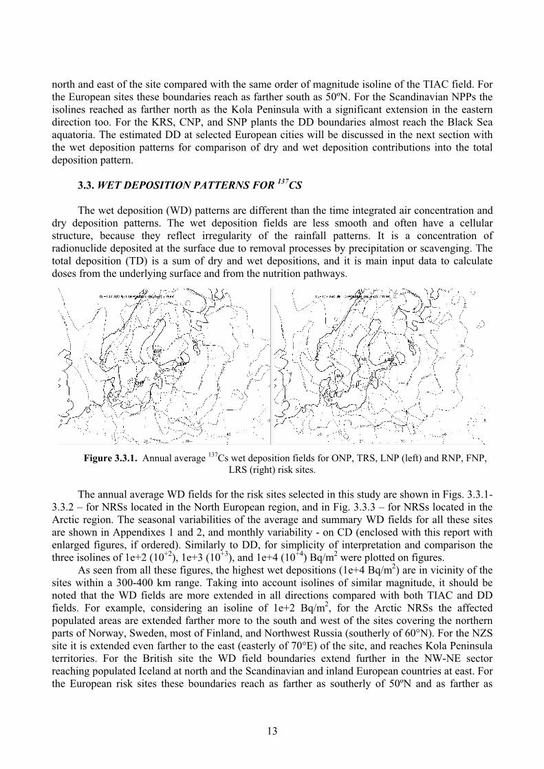
Figure 3.3.1. Annual average 137Cs wet deposition fields for ONP, TRS, LNP (left) and RNP, FNP,

LRS (right) risk sites.

The annual average WD fields for the risk sites selected in this study are shown in Figs. 3.3.1-

3.3.2 – for NRSs located in the North European region, and in Fig. 3.3.3 – for NRSs located in the

Arctic region. The seasonal variabilities of the average and summary WD fields for all these sites

are shown in Appendixes 1 and 2, and monthly variability - on CD (enclosed with this report with

enlarged figures, if ordered). Similarly to DD, for simplicity of interpretation and comparison the

three isolines of 1e+2 (10+2

), 1e+3 (10+3

), and 1e+4 (10+4

) Bq/m2 were plotted on figures.

As seen from all these figures, the highest wet depositions (1e+4 Bq/m2) are in vicinity of the

sites within a 300-400 km range. Taking into account isolines of similar magnitude, it should be

noted that the WD fields are more extended in all directions compared with both TIAC and DD

fields. For example, considering an isoline of 1e+2 Bq/m2, for the Arctic NRSs the affected

populated areas are extended farther more to the south and west of the sites covering the northern

parts of Norway, Sweden, most of Finland, and Northwest Russia (southerly of 60°N). For the NZS

site it is extended even farther to the east (easterly of 70°E) of the site, and reaches Kola Peninsula

territories. For the British site the WD field boundaries extend further in the NW-NE sector

reaching populated Iceland at north and the Scandinavian and inland European countries at east. For

the European risk sites these boundaries reach as farther as southerly of 50ºN and as farther as

14

easterly of 40ºE. For the Scandinavian NPPs the isolines reached as farther north as the Barents Sea

with a significant extension in the eastern direction passing through the 50ºE longitude. For the

KRS, CNP, and SNP plants the WD boundaries passed over the Black Sea aquatoria and almost

reached the Caspian Sea.

Figure 3.3.2. Annual average 137Cs wet deposition fields for BGP, INP, KRS (left) and BBP, BNP,

SNP, CNP (right) risk sites.

Figure 3.3.3. Annual average 137Cs wet deposition fields for KNS, KNP, and NZS risk sites.

Table 3.3.1. Annual average 137Cs dry, wet, and total depositions, and contribution of both dry and wet

depositions into total deposition at selected European cities resulted from the hypothetical release at the

Leningrad NPP.

City, Country

Dist to

LNP,

km

DD,

Bq/m2WD,

Bq/m2TD,

Bq/m2DD/TD,

%

WD/TD,

%Minsk, Belarus 673 2,01E+2 1,81E+2 3,83E+2 53 47

St.Petersburg, Russia 70 1,48E+4 3,45E+4 4,93E+4 30 70

Moscow, Russia 686 2,20E+2 4,75E+2 6,94E+2 32 68

Kiev, Ukraine 1057 3,70E+1 7,23E+1 1,09E+2 34 66

Stockholm, Sweden 618 1,88E+2 1,60E+2 3,48E+2 54 46

Oslo, Norway 1014 4,47E+1 1,60E+2 2,04E+2 22 78

Helsinki, Finland 424 2,85E+2 7,51E+2 1,04E+3 28 72

15

Copenhagen, Denmark 1077 8,10E+1 7,68E+1 1,58E+2 51 49

Vienna, Austria 1535 7,66E+0 1,43E+1 2,19E+1 35 65

Paris, France 2095 8,07E+0 3,20E+0 1,13E+1 72 28

London, UK 2025 1,14E+1 9,14E+0 2,06E+1 56 44

Brussels, Belgium 1840 1,67E+1 6,77E+0 2,35E+1 71 29

Berlin, Germany 1261 4,31E+1 5,21E+1 9,53E+1 45 55

Budapest, Hungary 1522 7,10E+0 4,26E+0 1,14E+1 62 38

Bucharest, Romania 1731 7,53E+0 4,07E+0 1,16E+1 65 35

Warszawa, Poland 983 4,32E+1 2,38E+1 6,71E+1 64 36

Praha, Czech Republic 1426 1,69E+1 2,75E+1 4,44E+1 38 62

Bratislava, Slovakia 1515 9,16E+0 1,37E+1 2,29E+1 40 60

Luxembourg, Luxembourg 1845 1,03E+1 4,08E+0 1,44E+1 72 28

Amsterdam, Netherlands 1699 1,70E+1 6,56E+0 2,36E+1 72 28

Reykjavik, Iceland 2625 6,43E-1 5,95E-1 1,24E+0 52 48

Dublin, Ireland 2246 6,73E-1 2,00E+0 2,67E+0 25 75

Bern, Switzerland 2012 2,03E+0 1,19E+1 1,39E+1 15 85

Tallinn, Estonia 245 9,70E+2 1,14E+3 2,11E+3 46 54

Riga, Latvia 435 3,43E+2 3,11E+2 6,54E+2 52 48

Vilnius, Lithuania 622 2,33E+2 1,52E+2 3,85E+2 61 39

Torshavn, Faeroes 1920 1,56E+0 1,39E+0 2,96E+0 61 39

Nuuk, Greenland 3939 5,17E-5 3,89E-5 9,06E-5 53 47

As shown in Tab. 3.3.1, on example of a hypothetical release from the Leningrad NPP, the

contribution of wet deposition vs. dry deposition into the total deposition vary significantly from

city to city. Among all considered capitals, 9 cities showed approximately equal contribution of

both depositions - 50±5%. The WD contribution is more than 70% of TD for another 8 cities

selected in this study. The DD contribution is more than 70% of TD for another 4 cities (i.e. twice

less than for WD), which are the Benelux countries and France and which are located farther west

from the LNP site. We should note that there is a peculiarity: at larger distances (more than 1000-

km) from the site the contribution of WD became greater.

3.4. GENERAL STATISTICS AND CORRELATIONS BETWEEN PATTERNS

In statistical analysis, if concentration of pollutants differing by orders of magnitude is

investigated than use of log-transformation for original data is considered as an important step.

Hence, all calculated 137

Cs TIAC, DD, and WD fields were initially log-transformed, and then

subsequent statistics was obtained. Let us consider descriptive statistics on example of the

Leningrad NPP.

Table 3.4.1. Descriptive statistics for the log-transformed annual average 137Cs time integrated air

concentration, dry, and wet deposition fields for the Leningrad NPP.

Field Range Min Max Mean Std. Dev Variance Skewness Kurtosis

Log10_TIAC 12,60 -6,00 6,60 0,88±0.01 2,33 5,41 -0,45±0.01 -0,34±0.03

Log10_DD 13,34 -6,00 7,34 1,57±0.01 2,38 5,65 -0,53±0.01 -0,12±0.03

Log10_WD 13,67 -6,00 7,67 1,79±0.01 2,39 5,71 -0,59±0.01 -0,03±0.03

A set of descriptive statistics - including range, variance, standard deviation, minimum and

maximum, and mean, skewness and kurtosis with a standard error - was calculated (Tab. 3.4.1). As

shown in Fig. 3.4.1, the given distribution histograms of log-transformed data for all fields have the

skewed (in the section of the lower values – to the left) nature. The vertical axis represents the

number of the cases when level of such concentration and depositions were observed. The

16

horizontal axis represents the log-transformed values of concentration – Log10_TIAC (in Bq·h/m3)

and depositions – Log10_DD and Log10_WD (in Bq/m2). As seen also from the table all

characteristics are higher for the wet deposition patterns compared with two others.

The correlations were estimated between TIAC, DD, and WD fields (Fig. 3.4.2). The best fit

of data was presented by the linear regression lines. All fields showed a statistically significant

(applying the 2-tailed test) strong positive correlation (with R2

0.972-0.999). The correlation

between TIAC and DD was higher (R 0.999) compared with correlation of these both with WD

(R 0.986). Such strong correlation between TIAC and DD also depend on, first of all, the

deposition parameterization scheme (employed in this version of the DERMA model), which uses a

limited number of the land-use categories.

(a) (b) (c)

Figure 3.4.1. Histograms of distribution of the log-transformed annual average 137Cs (horizontal axis

– magnitude, vs. vertical axis - # of cases) for a) time integrated air concentration, b) dry deposition, and c)

wet deposition fields for the Leningrad NPP.

Figure 3.4.2. Correlation between annual average 137Cs time integrated air concentration, dry, and

wet deposition fields.

Moreover, the concentration and depositions were evaluated as a function of a radial distance

from the Leningrad NPP as shown in Fig. 3.4.3. These were also evaluated using a box-plot

procedure with a division on seven distance classes (from 0 to 6 as shown on legend of Fig. 3.4.4).

The highest concentration and depositions are generally occurred within a first 1000-km range from

the LNP site with a low variability of one-two orders of magnitude. After 1500-km the range of

their variability became larger – within several (6-10) orders of magnitude, although the mean

17

decreased normally following the radioactive decay. The gap between classes 4 and 6, as seen on

figures and box-plots, shows differences in airflow patterns from the site. In particular, the higher

concentrations are more often observed to the south of the risk site (southerly of the LNP latitude –

59.90ºN) than to the north of the site, but after 4000km they became comparable. Similarly, it is for

the east (westerly of 29.0°E) compared with the west. It is important to say here that we focused on

the regional scale of the Northern Europe, and therefore, we limited our region of interest up to

4000-km from the site.

(a) (b) (c)

Figure 3.4.3. Annual average 137Cs a) time integrated air concentration, b) dry deposition, and c) wet

deposition fields (on a logarithmic scale) as a function of radial distance from the Leningrad NPP.

(a) (b) (c)

Figure 3.4.4. Box-plots of the annual average 137Cs patterns distribution for the a) time integrated air

concentration, b) dry deposition, and c) wet deposition fields for the Leningrad NPP as a function of the

distance class (0 - <500km, 1 – 500-1000km, 2 – 1000-2000km, 3 - 2000-3000km, 4 – 3000-4000km, 5 –

4000-5000km, 6 – >5000km).

On a seasonal scale, as shown in Fig. 3.4.5, the highest magnitude TIAC isolines (1e+3

Bq·h/m3) are concentrated around the sites and mostly they have a circle-oriented shape, although

for the British site, during summer it is significantly extended in the eastern direction and during

winter – in the north-western direction of the site (Fig. 3.4.5a). For the Ignalina site (Fig. 3.4.5b),

during summer it is more extended in the western direction, and during winter - in eastern direction.

The highest concentrations are more characteristic for the border regions of Lithuania, Latvia, and

Belarus. For the NZS site, during all seasons it is more concentrated in the NW-SW sector of the

site, and it is extended almost twice farther to the west compared with the east (Fig. 3.4.5c).

Similarly, the TIAC isolines of 1e+2 Bq·h/m3 are more extended in the directions of main

airflow from the sites and they have more an elliptical shape than a circle shape. For the BBP site

(Fig. 3.4.5a) during atmospheric transport such concentrations were not even observed at the

seashore of the European continent. These TIACs occurred mostly over the British Islands and

18

adjacent seas. For the Ignalina site (Fig. 3.4.5b), during summer the same isoline is more extended

(almost twice) in the western direction than during winter – in opposite, eastern direction of the site.

During spring, the extension is more pronounced along the NE-SW section. Among the

Scandinavian countries, the TIAC can reach magnitudes of 1e+2 Bq·h/m3 at the Baltic seashore

counties of Sweden only during summer, and south of Finland - only during spring. For NZS site

(Fig. 3.4.5c), during winter a significant extension in the NW direction from the site is occurred,

and during summer the area of the TIAC field is almost twice larger compared with all other

seasons. Throughout the year the populated Russian territories were practically unaffected by these

levels of concentration. Moreover, the seasonal variability of the NZS TIAC field varied within a 5

degree latitudinal belt.

(a) (b) (c)

Figure 3.4.5. Seasonal average 137Cs time integrated air concentration fields for the a) British NPPs,

b) Ignalina NPP, and c) Novaya Zemlya test site.

The further analyses of the seasonal DD and WD fields for the same NRSs (shown in Figs.

3.4.6-3.4.8) showed a more complex structure of the calculated fields, especially of the WD fields.

The dry deposition fields are significantly (especially during summer in the southern directions)

extended in all directions from the sites compared with the TIAC fields. The WD showed fields

with multiple cells. This reflected a cellular structure of the precipitation patterns. These fields are

also farther extended compared with the DD fields.

Figure 3.4.6. Seasonal average 137Cs dry (left) and wet (right) deposition fields for the British NPPs (BBP).

In particular, the multiple cells structure of wet deposition is well seen during all seasons for

the BBP site (Fig. 3.4.6) compared with the Ignalina and Novaya Zemlya sites. This multiplicity

depends strongly on the maritime climate peculiarities of the BBP site. The wet depositions as

higher as 1e+3 Bq/m2 are observed during winter-summer in the western part of Norway, during

19

winter – in Denmark, during fall – in Iceland and western seashore territories of Germany and

Benelux countries. The areas of wet depositions of 1e+2 Bq/m2 are extended to the south passing at

45ºN and to the east passing at 30ºE.

The multiple cells structure of wet deposition is less pronounced for the Ignalina NPP (Fig.

3.4.7). This site is more attributed to the inland site, and hence, it is related to more continental type

of the climate. During summer, although the dry deposition is higher in the E-S sector, the wet

deposition is more characteristic for the territories northerly of the site. During winter, the areas

enclosed by isolines of 1e+3 Bq/m2 are almost 2.5 larger for WD compared with DD field, and

these are more extended in the eastern directions from the site. Hence, throughout the year the dry

deposition of 1e+3 Bq/m2 is observed mostly over the Baltic States and northern Belarus. The wet

deposition of the same order of magnitude is characteristic for a wider area, especially during

winter, covering additionally territories of the Northwest Russia, Belarus, Ukraine, and Poland, as

well as extending farther into the Baltic Sea aquatoria. Cells of the local maxima for WD are more

often observed to the west of the site compared with the eastern directions (i.e. farther to the

Eurasian continent).

Figure 3.4.7. Seasonal average 137Cs dry (left) and wet (right) deposition fields for the Ignalina NPP (INP).

Figure 3.4.8. Seasonal average 137Cs dry (left) and wet (right) deposition fields for the Novaya Zemlya test

site (NZS).

For the Artic latitude site - Novaya Zemlya Archipelago (Fig. 3.4.8) - the wet deposition

pattern showed less variability in precipitation patterns. Although the WD fields are more extended

20

in all directions from the site compared with the DD fields, they have no well underlined patterns of

irregularity compared with other discussed sites. Throughout the year both depositions of 1e+3

Bq/m2

and higher magnitudes are not observed over populated Russian territories. During summer,

dry deposition of a lesser order of magnitude (1e+2 Bq/m2) can be observed over the Murmansk

and Archangelsk regions. The WD of the same magnitudes for the same regions is characteristic

during all seasons, although during winter-fall the areas enclosed by these isolines are more

extended farther to the Scandinavian Peninsula as well as during spring-summer they more

extended to the south of the site (up to 60ºN) over populated Russian territories.

The analysis of seasonal variability of the 137

Cs WD patterns at selected cities (Tab. 3.4.1)

showed that the deposition can be as much as 3.9 times higher during a particular season compared

with the average annual deposition. This is a characteristic situation in Dublin, Ireland during fall.

Among selected cities the lowest rate of maximum vs. average annual WD is 1.4 (Riga, Latvia).

Moreover, the rate of more than 3.0 is observed for cities located farther than a 1500-km circle from

the Leningrad plant. The minimum wet depositions are only characteristic during winter. This was

observed at 17 among 26 cities selected, and all of these are located farther than 600-km of the site.

The difference between the annual average and minimum varied up to 8 orders of magnitude at that

time, although this difference was only up to one order of magnitude when a minimum was

observed during other seasons.

Table 3.4.1. Seasonal variability of average 137Cs wet deposition patterns (Bq/m2) resulted from the

hypothetical release at the Leningrad NPP at selected European cities.

City, Country Dist to

LNP,

km

Spr Sum Fal Win Ann

Max

(seas)

Max

vs.

AnnMinsk, Belarus 673 2,79E+2 8,46E+1 2,30E+2 1,32E+2 1,81E+2 Spr 1,5

St.Petersburg, Russia 70 2,89E+4 1,68E+4 1,20E+4 8,03E+4 3,45E+4 Win 2,3

Moscow, Russia 686 8,32E+2 1,21E+2 5,80E+2 3,65E+2 4,75E+2 Spr 1,8

Kiev, Ukraine 1057 1,04E+1 1,26E+1 2,20E+2 4,58E+1 7,23E+1 Fal 2,9

Stockholm, Sweden 618 1,14E+2 1,19E+2 3,73E+2 3,32E+1 1,60E+2 Fal 2,3

Oslo, Norway 1014 2,54E+2 2,43E+2 1,31E+2 1,06E+1 1,60E+2 Spr 1,6

Helsinki, Finland 424 6,02E+1 5,71E+2 1,89E+3 4,78E+2 7,51E+2 Fal 2,5

Copenhagen, Denmark 1077 2,43E+1 1,59E+2 1,23E+2 2,12E-1 7,68E+1 Sum 2,1

Vienna, Austria 1535 1,34E+0 1,49E+0 5,43E+1 2,29E-4 1,43E+1 Fal 3,8

Paris, France 2095 1,15E+1 7,27E-1 5,52E-1 5,38E-5 3,20E+0 Spr 3,6

London, UK 2025 1,24E+1 4,52E+0 1,97E+1 3,34E-7 9,14E+0 Fal 2,2

Brussels, Belgium 1840 1,33E+1 1,12E+1 2,64E+0 1,62E-6 6,77E+0 Spr 2,0

Berlin, Germany 1261 1,87E+1 1,21E+2 6,56E+1 3,04E+0 5,21E+1 Sum 2,3

Budapest, Hungary 1522 1,58E+0 1,19E+0 1,42E+1 5,52E-2 4,26E+0 Fal 3,3

Bucharest, Romania 1731 4,21E+0 4,97E-1 1,07E+1 8,29E-1 4,07E+0 Fal 2,6

Warszawa, Poland 983 1,33E+1 5,23E+1 2,91E+1 6,32E-1 2,38E+1 Sum 2,2

Praha, Czech Republic 1426 9,94E-1 5,79E+1 5,11E+1 2,62E-2 2,75E+1 Sum 2,1

Bratislava, Slovakia 1515 2,38E+0 1,15E+1 4,09E+1 3,84E-3 1,37E+1 Fal 3,0

Luxembourg, Luxembourg 1845 1,91E+0 5,55E+0 8,85E+0 2,31E-5 4,08E+0 Fal 2,2

Amsterdam, Netherlands 1699 5,53E+0 1,30E+1 7,72E+0 1,66E-6 6,56E+0 Sum 2,0

Reykjavik, Iceland 2625 1,42E+0 6,10E-1 3,53E-1 9,87E-4 5,95E-1 Spr 2,4

Dublin, Ireland 2246 5,36E-2 2,03E-1 7,73E+0 2,05E-4 2,00E+0 Fal 3,9

Bern, Switzerland 2012 2,47E-1 1,78E+0 4,55E+1 6,78E-8 1,19E+1 Fal 3,8

Tallinn, Estonia 245 1,36E+2 6,37E+2 2,47E+3 1,30E+3 1,14E+3 Fal 2,2

Riga, Latvia 435 4,62E+2 1,68E+1 4,56E+2 3,09E+2 3,11E+2 Spr 1,4

Vilnius, Lithuania 622 1,14E+2 1,20E+2 2,36E+2 1,37E+2 1,52E+2 Fal 1,6

21

3.5. INDICATORS OF NRS IMPACT FOR EMERGENCY RESPONSE AND

PREPAREDNESS

Information about probabilistic spatial and temporal distribution of concentration, dry and wet

deposition patterns, especially during the fist day after an accident at NRS, could help the regional

authorities and decision makers to plan more effectively the system of operational monitoring and

emergency preparedness (i.e. to know: What areas are reachable during the first day after an

accident occurred at NRS? When different regions, counties, administrative units, etc. should be

ready for countermeasures after an accident/event at risk sites?). It should be noted that some

estimates based on evaluation of only atmospheric transport from the sites were done by Mahura &

Baklanov, 2002. They introduced a set of the NRS impact indicators to characterize peculiarities of

the first day: fast transport (FT) probability fields, maximum reaching distance (MRD), maximum

possible impact zone (MPIZ), and typical transport time (TTT) fields. Here, we will focus on

estimates based on evaluation of both radionuclide transport and deposition patterns. Let us

consider the British NRS as an example.

The annual average fields during the first day of atmospheric transport from the block of the

British NPPs (BBP) are shown in Fig. 3.5.1a - for the time integrated air concentration of 137

Cs, in

Fig. 3.5.1b – for the dry deposition of 137

Cs, and in Fig. 3.5.1c – for the wet deposition of 137

Cs. The

seasonal variability of these three fields is shown in Fig. 3.5.2. The BBP site is geographically

located on the British Islands. Hence, the atmospheric transport, dispersion, and deposition of

radionuclides will strongly depend on the peculiarities of the maritime climate of these islands.

(a) (b) (c)

Figure 3.5.1. Annual average 137Cs a) time integrated air concentration, b) dry deposition, and c) wet

deposition fields during the first day of atmospheric transport from the British NPPs (BBP).

On an annual scale (Fig. 3.5.1), the higher values of concentration and depositions of 137

Cs are

occurred more often to the north of the site compared with the southern directions. It is attributed to

the prevailing atmospheric patterns associated with the Icelandic Low activities and proximity to

the Gulf Stream current. For the WD field the annual areas, enclosed by the first three highest

isolines of 1e+4, 1e+3, and 1e+2 Bq/m2, are almost 2.5 times larger compared with the DD field.

The higher values and larger areas for the wet deposition patterns, resulted from atmospheric

transport from this site, depend on a frequent precipitation in this region as well as specifity of the

maritime boundary layer which suppresses a deposition at the surface. During the first day, the

British Islands and surrounding seas are mainly affected by the highest concentration and

depositions ranging within 1e+3-1e+2 (Bq·h/m3) and 1e+4-1e+3 (Bq/m

2), respectively. Among the

populated European regions, only territories of countries situated along the seashore of the North

Sea aquatoria, including Denmark, are at the higher risk compared with other countries. For most of

the Western Europe countries, the TIAC of 137

Cs will be less than 1e+0 Bq·h/m3, except Denmark,

Northwest Germany, Benelux countries, and western territories of Norway. For the same territories,

22

the dry deposition is about of 1e+1 (Bq/m2) and the wet deposition is twice higher (i.e. it is about of

1e+2 Bq/m2).

Let us consider TIAC, DD, WD, and total deposition (TD) at selected geographical locations

(capitals of the European countries situated northerly than 45ºN).

Table 3.5.1. Annual average 137Cs time integrated air concentration, dry, wet, and total depositions

during the first day of atmospheric transport at selected European cities resulted from the hypothetical

release at the British NPPs.

# City, Country

Dist to

LNP,

km

TIAC,

Bq·h/m3DD,

Bq/m2WD,

Bq/m2TD,

Bq/m2

DD/

TD,

%

WD/

TD,

%1 Copenhagen, Denmark 1029 1,18E+0 6,36E+0 6,25E+1 6,89E+1 9 91

2 Helsinki, Finland 1622 3,97E-5 2,15E-4 1,25E-3 1,46E-3 15 85

3 Oslo, Norway 1045 5,16E-1 2,79E+0 1,14E+1 1,42E+1 20 80

4 Stockholm, Sweden 1406 4,50E-2 2,43E-1 1,41E+0 1,65E+0 15 85

5 Reykjavik, Iceland 1488 1,24E-4 6,71E-4 1,22E-2 1,29E-2 5 95

6 Torshavn, Faeroes 859 1,73E+0 9,33E+0 5,25E+1 6,19E+1 15 85

7 Nuuk, Greenland 2847 0,00E+0 0,00E+0 0,00E+0 0,00E+0 0 0

8 Minsk, Belarus 2005 1,04E-2 5,59E-2 8,29E-1 8,85E-1 6 94

9 St.Petersburg, Russia 2095 6,09E-17 3,29E-16 9,18E-15 9,51E-15 3 97

10 Moscow, Russia 2577 0,00E+0 0,00E+0 0,00E+0 0,00E+0 0 0

11 Kiev, Ukraine 2324 5,59E-10 3,02E-9 1,42E-8 1,72E-8 18 82

12 Vienna, Austria 1540 4,75E-5 2,57E-4 2,67E-5 2,83E-4 91 9

13 Paris, France 744 4,07E-1 2,20E+0 5,55E+0 7,75E+0 28 72

14 London, UK 402 1,52E+1 8,22E+1 1,25E+2 2,07E+2 40 60

15 Brussels, Belgium 667 4,13E+0 2,23E+1 5,14E+1 7,37E+1 30 70

16 Berlin, Germany 1136 5,66E-1 3,06E+0 2,70E+1 3,01E+1 10 90

17 Budapest, Hungary 1751 1,71E-8 9,23E-8 1,29E-13 9,23E-8 100 0

18 Bucharest, Romania 2389 0,00E+0 0,00E+0 0,00E+0 0,00E+0 0 0

19 Warszawa, Poland 1636 3,81E-2 2,06E-1 4,27E+0 4,48E+0 5 95

20 Praha, Czech Republic 1312 5,06E-2 2,73E-1 2,42E+0 2,69E+0 10 90

21 Bratislava, Slovakia 1589 2,97E-4 1,60E-3 1,38E-4 1,74E-3 92 8

22 Luxembourg, Luxembourg 852 4,65E-1 2,51E+0 1,59E+1 1,84E+1 14 86

23 Amsterdam, Netherlands 606 7,53E+0 4,06E+1 2,38E+2 2,78E+2 15 85

24 Dublin, Ireland 222 6,16E+1 3,33E+2 3,26E+2 6,58E+2 51 49

25 Bern, Switzerland 1141 1,22E-4 6,56E-4 1,43E-2 1,50E-2 4 96

26 Tallinn, Estonia 1781 4,42E-7 2,39E-6 1,88E-5 2,12E-5 11 89

27 Riga, Latvia 1737 1,27E-3 6,83E-3 2,64E-1 2,71E-1 3 97

28 Vilnius, Lithuania 1844 1,90E-2 1,03E-1 3,66E+0 3,76E+0 3 97

29 BBP, UK 0 4,48E+3 2,42E+4 2,53E+4 4,95E+4 49 51

As seen from Tab. 3.5.1 the highest values for the concentration and depositions (1e+3 and

1e+4 orders of magnitude, respectively) are in vicinity of the BBP site. During the first day the

contribution of the wet deposition into the total deposition is several times higher for most of the

selected cities, except Vienna and Bratislava. The WD contribution is almost equal to the DD

contribution at Dublin and the BBP site. For three cities – Moscow, Nuuk, and Bucharest – for both

contributions it is equal to 0 (i.e. cities were not reachable during the first day of atmospheric

transport) because the limited duration (5-days) of trajectories considered. For cities situated within

a 1000-km circle around the BBP site, the concentration decreased by several orders of magnitude:

from 1e+3 to 1e-1 Bq·h/m3.

23

On a seasonal scale (Fig. 3.5.2), during summer the areas of the TIAC, DD, and WD fields are

smaller compared with other seasons, and they are more concentrated around the BBP site.

Moreover, these fields are also less extended in the eastern sector from the site, although in other

seasons there is a significant propagation of the isolines in the eastern directions. During fall, the

Scandinavian Peninsula countries are minimally affected by atmospheric transport and deposition

from the site, the contours of the fields are more extended in the NW-SE direction (passing over the

Faeroe Islands and Scandinavian countries) compared with others. During winter, the WD pattern is

significantly propagated in the inland European countries.

Finally, analysis of such TIAC, DD, and WD fields could be used in the emergency response

systems for accidental releases of radioactivity. These fields allow an estimation of transport times,

boundaries of possible maximal contamination, integrated concentrations, dry and wet deposition

patterns, geographically farthest territories reachable by a contaminated cloud during selected time

(for example, every 3 hour) atmospheric transport from the risk sites to/over a particular

geographical territory, region, country, city, etc. This information is one of the important input

parameters for the decision-making process.

(Spr) (Spr) (Spr)

(Sum) (Sum) (Sum)

(Fal) (Fal) (Fal)

24

(Win) (Win) (Win)

Figure 3.5.2. Seasonal average 137Cs time integrated air concentration (left), dry deposition (middle), and

wet deposition (right) fields during the first day of atmospheric transport from the British NPPs.

It should be reminded also that the BBP site consisted of several nuclear risk sources

including the Sellafield nuclear processing plant. Hence, the results obtained for the BBP site will

be similar if modelling will be performed for the exact geographical location of the mentioned

processing plant. It is assumed to be valid due to short distance between the coordinates of the BBP

site and Sellafield plant as well as due to similarities of the characteristic mesoscale patterns over

the geographical region of both sites’ locations.

3.6. SPECIFIC CASE STUDIES FOR 137

CS,131

I,90

SR, AND 85

KR RELEASES

In comparison with the long-term dispersion modelling, the specific case studies have some

peculiarities and criteria for selection discussed by Baklanov et al., 2002b. The specific case study

approach is computationally less expensive compared with the dispersion modelling for a multiyear

period, although it allows considering further risk and vulnerability analysis only on particular

dates. Alternatively, this approach provides possibility to see potential consequences of an accident

for worst-case meteorological situations. Some case studies with evaluation of possible

consequences were considered for the Kola nuclear power plant (Baklanov et al., 2002a) and

nuclear submarine bases of the Russian Northern and Pacific Fleets (Bergman et al., 1998;

Baklanov et al., 2002b; Mahura et al., 2002; Baklanov et al., 2003).

The selection of specific cases with typical or worst-case scenarios can be based on results

from trajectory modelling and probability fields analysis. In general, at least, four criteria could be

used for specific case selection. First, the direction of atmospheric transport of radioactive cloud

after an accidental release at NRS should be toward the region of interest. In our study, these

regions are countries and populated territories of the Euro-Arctic region. Second, the possibility of

precipitation during atmospheric transport of the radioactive cloud over the region of interest should

be taken into account. In our study it could be inferred from the dispersion modelling of wet

deposition patterns. Third, the relatively short travel time of the radionuclide cloud from the NRS

location toward the region of interest will be important. Fourth, the relatively large coverage of the

regions of interest by the radioactive cloud during atmospheric transport should be considered.

In this section of report, we will consider two specific cases in more details. These cases are:

A) 24th

August 2000, and B) 10th

April 2002. For these cases, we evaluated atmospheric transport,

dispersion, and deposition of the following radionuclides - 137

Cs,131

I,90

Sr,95

Kr - for the discrete

continuous unit hypothetical release (DUHR) with a fixed rate of 1·1011

Bq/s. Hence, the total

amount of radioactivity released during a one-day release is equal to

1·1011

(Bq/s)·24(hour)·60(min)·60(sec) = 8.64·1015

(Bq). For simplification let us suggest this

25

amount to be the same for all radionuclides. We do not consider any specific accident scenario but

our simulation results can be easily recalculated for any scenario of accident. Moreover, we did not

consider different release heights because such sensitivity studies were done by Bergman et al.,

1998; Baklanov et al., 2001.

Specific Case A: Leningrad NPP, 24 August 2000

For this specific case of 24 August 2000, we analyzed atmospheric transport of three

radionuclides (137

Cs,131

I, and 90

Sr – as major dose-contributing radionuclides) for DUHR occurred

during 24 hours (24-25 Aug 2000, 00 UTC) at the Leningrad NPP, Russia. As input meteorological

data the ECMWF model output was used. Following the subsequent temporal daily snapshots of

radionuclide concentration it is possible to identify propagation of the radionuclide cloud.

(1 day) (2 day) (3 day)

(4 day) (5 day) (6 day)

Figure 3.6.1. 90Sr air concentration fields for DUHR occurred during 24-25 Aug 2000, 00 UTC from the

Leningrad NPP.

During the first two days, atmospheric transport generally occurred in the eastern direction

from the site as shown in Figs. 3.6.1 and 3.6.2 for 90

Sr and 131

I, respectively. During the 3rd

day, the

contaminated cloud continued motion by westerlies, although a transport in the western direction is

also became pronounced. During the 4th

day, since release occurred at the LNP site, the directions

of the separated cloud transport did not change significantly, except that the southern component

became evident. During the 5th

and 6th

days, a part of the radionuclide cloud, initially moved in the

eastern direction, propagated to the south passing over territories of the Black Sea and Ukraine.

Other part of the cloud, previously moved in the western direction, travelled to the north passing

over territories of the Scandinavian countries.

Comparison of 90

Sr and 131

I (long-lived vs. short-lived radionuclide) showed a significant

decrease of concentration during atmospheric transport. This especially is seen at the last two days

(5 and 6). Only small areas over the Scandinavian Peninsula and Black Sea were still affected by

26

the presence of 131

I on the 6th

day, although for 90

Sr, the affected area remained relatively large

extending from the southern territories of the Scandinavian Peninsula to the Black Sea.

(1 day) (2 day) (3 day)

(4 day) (5 day) (6 day)

Figure 3.6.2. 131I air concentration fields for DUHR occurred during 24-25 Aug 2000, 00 UTC from the

Leningrad NPP.

(a) (b) (c)

Figure 3.6.3. Time integrated air concentration fields of a) 137Cs, b) 131I, and c) 90Sr on 6th day of

atmospheric transport from the Leningrad NPP for DUHR occurred during 24-25 Aug 2000, 00 UTC.

The TIAC fields for all three radionuclides are shown in Fig. 3.6.3. The shape and structure of

TIAC are similar for nuclides: 137

Cs and 90

Sr. The correlation coefficient between these two fields is

0.98. It is not a surprise because it is strongly dependent on the half-life of the nuclides

(9.50428·108

sec vs. 9.17640·108

sec for 137

Cs vs. 90

Sr, respectively) used in modelling of

radioactive decay processes. Similar conclusion can be made about the DD fields shown in Fig.

3.6.4. Since the Leningrad NPP site is an inland site, the more continental type of the climate than

the maritime is a peculiarity of this site compared, for example, with the Sellafield processing plant

(discussed in §3.5). The strong dependence on the precipitation irregularity presence during

27

atmospheric transport of the contaminated cloud is reflected in the wet deposition patterns. Hence,

the structure of the WD field is more cellular compared with TIAC and DD. The total area enclosed

by the WD isolines is much smaller too (Fig. 3.6.5).

(a) (b) (c)

Figure 3.6.4. Dry deposition fields of a) 137Cs, b) 131I, and c) 90Sr on 6th day of atmospheric transport from

the Leningrad NPP for DUHR occurred during 24-25 Aug 2000, 00 UTC.

Analyses of fields (shown in Figs 3.6.1-3.6.5) allow identifying several features for this

specific case. First, it should be noted that for 137

Cs and90

Sr the shape and magnitude of isolines are

similar for all fields, and it is due to almost the same half-life times and reference dry deposition

velocities for these radionuclides compared with 131

I. Second, for 131

I, the surface air concentration

decreases faster with distance from the site (similar with other calculated fields, although the rate of

decrease is slower). Additionally, an area under a particular order of magnitude isoline could be

calculated similarly to estimation of areas enclosed by isolines of the maximum reaching distance

and maximum possible impact zone indicators (based on results of trajectory modelling, see

Mahura & Baklanov, 2002).

(a) (b) (c)

Figure 3.6.5. Wet deposition fields of a) 137Cs, b) 131I, and c) 90Sr on 6th day of atmospheric transport from

the Leningrad NPP for DUHR occurred during 24-25 Aug 2000, 00 UTC.

If several geographical locations of interest are selected (i.e. its latitude and longitude are

known) than exact values of the time integrated air concentration, dry deposition, and wet

deposition can be calculated by interpolation from the original fields. Let us evaluate TIAC, DD,

and WD (shown in Tab. 3.6.1 and 3.6.2) at locations of the selected European cities after 5 days of

atmospheric transport from the Leningrad NPP.

The highest 137

Cs TIAC (1.61e+2 Bq·h/m3) was at Copenhagen, Denmark and the lowest –

4.95e-4 Bq·h/m3

- was at Riga, Latvia. Similarly, the highest 90

Sr TIAC – 1.16e+2 Bq·h/m3

- at

Copenhagen, Denmark, and the lowest - 2.98e-4 Bq·h/m3

- at Riga, Latvia. But, although the lowest

28

131I TIAC (3.33e-6 Bq·h/m

3) was at Riga, Latvia; the highest – 1.74e+1 Bq·h/m

3- at Minsk,

Belarus. The similar situation is for the DD patterns vs. radionuclides, i.e. the highest and lowest

magnitudes of DD for a particular radionuclide were observed at the same cities as for the

concentrations. The lower TIACs and DDs for three cities – Budapest, Tallinn, and Riga – is a

result of latter arrival of the contaminated cloud to these locations compared with other cities.

Table 3.6.1. Estimated time integrated air concentration of radionuclides at selected cites for DUHR

occurred (24-25 Aug, 2000, 00 UTC) at the Leningrad NPP.

Time Integrated Air

Concentration (TIAC), Bq·h/m3City, Country Lat, ° Long, °

Distance

to LNP,

km Cs137 131I 90Sr

St.Petersburg, Russia 59.89 30.26 70 9,49E+0 8,48E+0 9,39E+0

Tallinn, Estonia 59.43 24.73 245 1,86E-3 9,87E-6 1,10E-3

Helsinki, Finland 60.60 21.43 424 5,50E-1 3,03E-3 3,24E-1

Riga, Latvia 56.95 24.10 435 4,95E-4 3,33E-6 2,98E-4

Stockholm, Sweden 59.33 18.05 618 1,52E+1 1,81E-1 9,67E+0

Vilnius, Lithuania 54.67 25.32 622 6,72E+1 1,30E+1 5,69E+1

Minsk, Belarus 53.90 27.57 673 1,21E+2 1,74E+1 9,88E+1

Moscow, Russia 55.75 37.58 686 3,48E+1 5,00E+0 2,82E+1

Warszawa, Poland 52.25 21.00 983 1,41E+2 8,10E+0 1,03E+2

Oslo, Norway 59.92 10.75 1014 2,60E+1 5,15E-1 1,76E+1

Kiev, Ukraine 50.43 30.52 1057 3,13E+1 5,19E-1 2,06E+1

Copenhagen, Denmark 55.67 12.58 1077 1,61E+2 6,23E+0 1,16E+2

Berlin, Germany 52.52 13.40 1261 1,36E+2 8,57E+0 1,03E+2

Praha, Czech Republic 50.08 14.47 1426 3,91E+0 3,16E-1 3,04E+0

Bratislava, Slovakia 48.15 17.12 1515 4,82E-2 4,54E-3 3,80E-2

Budapest, Hungary 47.50 19.08 1522 2,61E-3 9,55E-6 1,47E-3

Vienna, Austria 48.20 16.37 1535 6,65E-3 5,85E-4 5,22E-3

Bucharest, Romania 44.43 26.10 1731 1,30E-1 1,24E-3 8,18E-2

Table 3.6.2. Estimated dry and wet depositions, and percentage contribution of wet deposition of

radionuclides at selected cites for DUHR occurred (24-25 Aug, 2000, 00 UTC) at the Leningrad NPP.

Dry Deposition

(Bq/m2)

Wet Deposition

(Bq/m2)

Wet Deposition/

Total Deposition,

%

City, Country

Cs137 131I 90Sr Cs137 131I 90Sr Cs137 131I 90Sr

St.Petersburg, Russia 5,13E+1 1,18E+2 6,76E+1 9,85E-2 5,72E-2 9,75E-2 0,2 <0,1 0,1

Tallinn, Estonia 1,01E-2 2,11E-4 7,90E-3 0,00E+0 0,00E+0 0,00E+0 <0,1 <0,1 0,0

Helsinki, Finland 2,97E+0 6,50E-2 2,33E+0 3,31E-3 1,82E-5 1,95E-3 0,1 <0,1 0,1

Riga, Latvia 2,67E-3 6,93E-5 2,15E-3 7,63E-7 3,76E-9 4,45E-7 <0,1 <0,1 <0,1

Stockholm, Sweden 8,20E+1 3,84E+0 6,96E+1 9,99E-5 2,92E-6 7,08E-5 <0,1 <0,1 <0,1

Vilnius, Lithuania 3,63E+2 2,07E+2 4,09E+2 3,34E+1 5,06E+0 2,84E+1 8,4 2,4 6,5

Minsk, Belarus 6,51E+2 2,83E+2 7,11E+2 3,92E+1 4,59E+0 3,25E+1 5,7 1,6 4,4

Moscow, Russia 1,88E+2 7,85E+1 2,03E+2 1,38E-2 5,09E-4 1,01E-2 <0,1 <0,1 <0,1

Warszawa, Poland 7,64E+2 1,43E+2 7,42E+2 8,62E+0 4,44E-1 6,47E+0 1,1 0,3 0,9

Oslo, Norway 1,40E+2 1,05E+1 1,26E+2 1,20E+0 2,13E-2 8,05E-1 0,8 0,2 0,6

Kiev, Ukraine 1,69E+2 1,01E+1 1,49E+2 4,25E+0 6,03E-2 2,79E+0 2,5 0,6 1,8

29

Copenhagen, Denmark 8,68E+2 1,20E+2 8,36E+2 9,75E+0 4,14E-1 7,21E+0 1,1 0,3 0,9

Berlin, Germany 7,32E+2 1,57E+2 7,41E+2 7,87E+1 4,57E+0 6,03E+1 9,7 2,8 7,5

Praha, Czech Republic 2,11E+1 5,63E+0 2,19E+1 1,50E+0 1,03E-1 1,17E+0 6,6 1,8 5,1

Bratislava, Slovakia 2,60E-1 7,87E-2 2,74E-1 6,71E-3 4,91E-4 5,28E-3 2,5 0,6 1,9

Budapest, Hungary 1,41E-2 2,05E-4 1,06E-2 1,56E-4 5,53E-7 8,78E-5 1,1 0,3 0,8

Vienna, Austria 3,59E-2 1,03E-2 3,75E-2 2,28E-3 1,64E-4 1,79E-3 6,0 1,6 4,6

Bucharest, Romania 7,04E-1 2,66E-2 5,89E-1 1,26E-3 1,19E-5 7,90E-4 0,2 <0,1 0,1

The highest 137

Cs WD (7.87e+1 Bq/m2) was at Berlin, Germany and the lowest (7.63e-7

Bq/m2) was at Riga, Latvia (considering that at Tallinn, Estonia the wet deposition did not even

occur). Similarly, the highest 90

Sr WD (6.03e+1 Bq/m2) - at Berlin, Germany and the lowest –

4.45e-7 Bq/m2

- at Riga, Latvia. But, although the lowest 131

I WD (3.76e-9 Bq/m2) was at Riga,

Latvia, the highest – 5.06e+0 Bq/m2

- at Vilnius, Lithuania. For this specific case, the contribution

of wet deposition during atmospheric transport was, in general, negligible ranging from less than

0.1 (shown in Tab. 3.6.2 as <0.1 or negligible) to 9.7% of the total deposition. Because of the

natural (following the radioactive decay) faster decrease of 131

I TIAC, especially during the first

days of transport, the TIAC, DD, WD, and contribution of wet deposition were also several times

lesser compared with other radionuclides. Hence, for this particular specific case the precipitation

factor was not a significant contributor, and major role was played by the atmospheric transport,

diffusion, and dry deposition.

Specific Case B: Chernobyl NPP, 10 April 2002

For this specific case of 10 Apr 2002, we analyzed atmospheric transport of three

radionuclides (137

Cs,131

I, and 85

Kr) for the discrete unit hypothetical releases (DUHR) of two

variants occurred within 10-11 Apr 2002 at the Chernobyl NPP, Ukraine. As input meteorological

data the DMI-HIRLAM model output was used. For comparative purposes two versions of the

DMI-HIRLAM model were run: E-version (resolution of 0.15º) and G-version (resolution of 0.45º)

- as shown in Figs. 3.6.6-3.6.7. Also, the hypothetical releases of two different durations were also

studied: 24 hours (variant 1) and 3 hours (variant 2) occurred during 10-11 Apr 2002 – as shown in

Figs. 3.6.6-3.6.7. The total amount of radioactivity released during 3 hours is equal to 3.78·1014

Bq,

and for 24 hour release – 8.64·1015

Bq.

(E-version of the DMI-HIRLAM model)

30

(G-version of the DMI-HIRLAM model)

Figure 3.6.6. 137Cs air concentration (left), dry deposition (middle), and wet deposition (right) fields at 12

Apr 2002, 12 UTC for DUHR occurred during 24 hours (10-11 Apr 2002, 12 UTC) at the Chernobyl NPP.

The snapshots of calculated fields for the radionuclide 137

Cs air concentration, dry deposition,

and wet deposition were taken after 2 days of atmospheric transport (i.e. at 12 Apr 2002, 12 UTC)

since releases of both durations started at the Chernobyl site (i.e. at 10 Apr 2002, 12 UTC). During

these two days, this specific case clearly showed the atmospheric transport in the north-western

direction and deposition over territories of Belarus, eastern Poland, Baltic States, and southern parts

of Sweden and Finland. After the first two days transport continued over the Scandinavian

Peninsula and regions of the North-West Russia. Considering the similar magnitude isolines, it is

well seen that the total area covered by the contaminated cloud is larger when a longer duration

release is evaluated. In particular, the area of 137

Cs air concentration field (left plate in Fig. 3.6.7) is

more than two times smaller compared with one day release (left plat in Fig. 3.6.6).

(E-version of the DMI-HIRLAM model)

(G-version of the DMI-HIRLAM model)

Figure 3.6.7. 137Cs air concentration (left), dry deposition (middle), and wet deposition (right) fields at 12

Apr 2002, 12 UTC for DUHR occurred during 3 hours (10 Apr 2002, 12-15 UTC) at the Chernobyl NPP.

31

Similarly, although less pronounced, the areas are larger for the dry and wet deposition fields

shown in the middle and right plates of the same figures. It should be noted that the dry and wet

deposition fields resemble each other by the shape, although the wet deposition field has more

cellular structure, due to irregularity of rainfall patterns during transport over the studied region.

The differences in the shapes of all patterns (considering results of the E and G versions), especially

of the wet deposition pattern, strongly depend on the model resolution. In particular, in E-version

the precipitation processes during atmospheric transport will be resolved more accurate, although in

G-version these fields are more smoothed loosing some aspects of the rainfall irregularity.

The air concentration fields for three selected radionuclides at different time intervals for a

one day release are shown in Fig. 3.6.8. The snapshots are given at 12, 13, and 14 Apr of 2002, 12

UTC. As seen from the figure, initially the atmospheric transport from the nuclear plant occurred in

the north-western direction passing over territories of Belarus, Poland, and Baltic States. At 12 Apr

2002, the contaminated cloud reached an aquatoria of the Baltic Sea. During the next day - 13 Apr

2002 – the transport shifted in the northern, and then in the north-eastern directions passing over the

aquatoria of the Baltic Sea and surrounding sea countries of the Scandinavian Peninsula and Baltic

region. During the fourth day – 14 Apr 2002 – the cloud continued extension in the western and

north-eastern directions passing over the Scandinavian Peninsula territories.

As seen from the figure, during the first days of transport the air concentration of 131

I

decreased significantly compared with other nuclides. Concentration of this nuclide varied between

1e-3-1e-2 Bq·h/m3

after 4 days of transport since release started at the site. The highest

concentration is observed over the central aquatoria of the Baltic Sea and territories of Sweden and

Finland adjacent to this aquatoria. Similar area with higher concentrations is for 137

Cs, although the

concentration levels will be two orders of magnitude higher. Because 85

Kr, as a noble gas, does not

account deposition processes during transport, the highest – 1e+1 Bq·h/m3

- concentration of

krypton remained if compared with other nuclides, as well as the area enclosed by the isolines

remained the largest.

137Cs

32

131I

85Kr

Figure 3.6.8. Radionuclide (top plate – 137Cs; middle plate - 131I; bottom plate - 85Kr) air concentration fields

at 00 UTC of 12 Apr 2002 (left), 13 Apr 2002 (middle), and 14 Apr 2002 (right) for DUHR occurred during

24 hours (10-11 Apr 2002, 12 UTC) at the Chernobyl NPP.

The time integrated air concentrations of radionuclides at 14 Apr 2002, 00 UTC for the same

release at the Chernobyl NPP are shown in Fig. 3.6.9. Because both 137

Cs and 131

I undergo the

deposition processes the areas enclosed by the highest TIAC isoline (1e+2 Bq·h/m3) will be

significantly smaller compared with 85

Kr. The highest TIAC for 137

Cs will be less frequent over the

populated territories of the Scandinavian Peninsula than for 85

Kr. Moreover, the TIAC of 131

I will

be less by an order of magnitude compared with both 137

Cs and 85

Kr.

The total deposition fields (as a sum of dry and wet depositions) of radionuclides at 14 Apr

2002, 00 UTC for the same release at the Chernobyl NPP are shown in Fig. 3.6.10. Only deposition

for two nuclides - 137

Cs and 131

I – was considered because for noble gases a deposition is not

included. The area of the fields enclosed by the lowest isoline of 100 Bq/m

2 is larger for

137Cs

compared with 131

I due to significant differences in deposition velocities and life-times of these

nuclides. The higher deposition levels, ranging from 1e+2 to 1e+4 Bq/m2, are observed 1) in

vicinity of the Chernobyl NPP following the north-western direction of atmospheric transport

during the first day, and 2) over the populated territories of the Baltic States, Belarus, and

Scandinavian Peninsula (Sweden and Finland).

33

(a) (b) (c)

Figure 3.6.9. Time integrated air concentration fields of a) 137Cs, b) 131I, and c) 85Kr at 14 Apr 2002, 00

UTC for DUHR occurred during 24 hours (10-11 Apr 2002, 12 UTC) at the Chernobyl NPP.

(a) (b)

Figure 3.6.10. Total deposition fields of a) 137Cs and b) 131I at 14 Apr 2002, 00 UTC for DUHR occurred

during 24 hours (10-11 Apr 2002, 12 UTC) at the Chernobyl NPP.

3.7. ESTIMATION OF POTENTIAL IMPACT AT COPENHAGEN, DENMARK DUE TO

RELEASES AT SELECTED NUCLEAR RISK SITES

As an example, let us estimate a potential impact of the NRSs’ hypothetical releases on one of

the Nordic countries’ capitals – Copenhagen, Denmark. The results of long-term modelling of

atmospheric transport, dispersion, and deposition patterns represented by the TIAC, DD, and WD

fields were used to evaluate the annual average levels concentration and depositions of 137

Cs and

ranking of potential impact from selected in this study NRSs on the city. As shown in Tab. 3.7.1,

four risk sites are located within a 500-km circle around Copenhagen: Barsebaeck, Ringhals,

Oskarshamn NPPs of Sweden and the block of the German NPPs. For these sites, the estimated

TIAC at Copenhagen varied between 1e+3–1e+2 Bq·h/m3

and depositions are 1e+4-1e+2 Bq/m2.

The contribution of the wet deposition into the total deposition pattern varies between 46 and 76%.

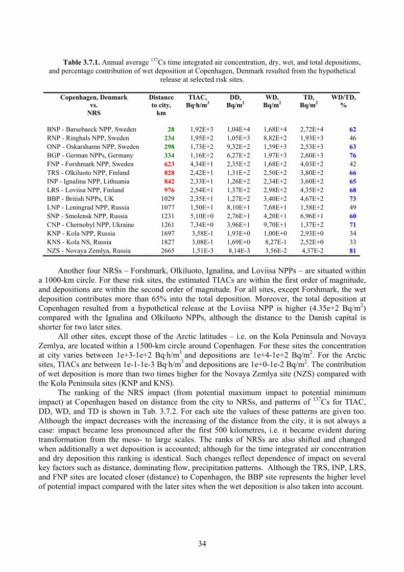
34

Table 3.7.1. Annual average 137Cs time integrated air concentration, dry, wet, and total depositions,

and percentage contribution of wet deposition at Copenhagen, Denmark resulted from the hypothetical

release at selected risk sites.

Copenhagen, Denmark

vs.

NRS

Distance

to city,

km

TIAC,

Bq·h/m3DD,

Bq/m2WD,

Bq/m2TD,

Bq/m2WD/TD,

%

BNP - Barsebaeck NPP, Sweden 28 1,92E+3 1,04E+4 1,68E+4 2,72E+4 62

RNP - Ringhals NPP, Sweden 234 1,95E+2 1,05E+3 8,82E+2 1,93E+3 46

ONP - Oskarshamn NPP, Sweden 298 1,73E+2 9,32E+2 1,59E+3 2,53E+3 63

BGP - German NPPs, Germany 334 1,16E+2 6,27E+2 1,97E+3 2,60E+3 76

FNP - Forshmark NPP, Sweden 623 4,34E+1 2,35E+2 1,68E+2 4,03E+2 42

TRS - Olkiluoto NPP, Finland 828 2,42E+1 1,31E+2 2,50E+2 3,80E+2 66

INP - Ignalina NPP, Lithuania 842 2,33E+1 1,26E+2 2,34E+2 3,60E+2 65

LRS - Loviisa NPP, Finland 976 2,54E+1 1,37E+2 2,98E+2 4,35E+2 68

BBP - British NPPs, UK 1029 2,35E+1 1,27E+2 3,40E+2 4,67E+2 73

LNP - Leningrad NPP, Russia 1077 1,50E+1 8,10E+1 7,68E+1 1,58E+2 49

SNP - Smolensk NPP, Russia 1231 5,10E+0 2,76E+1 4,20E+1 6,96E+1 60

CNP - Chernobyl NPP, Ukraine 1261 7,34E+0 3,96E+1 9,70E+1 1,37E+2 71

KNP - Kola NPP, Russia 1697 3,58E-1 1,93E+0 1,00E+0 2,93E+0 34

KNS - Kola NS, Russia 1827 3,08E-1 1,69E+0 8,27E-1 2,52E+0 33

NZS - Novaya Zemlya, Russia 2665 1,51E-3 8,14E-3 3,56E-2 4,37E-2 81

Another four NRSs – Forshmark, Olkiluoto, Ignalina, and Loviisa NPPs – are situated within

a 1000-km circle. For these risk sites, the estimated TIACs are within the first order of magnitude,

and depositions are within the second order of magnitude. For all sites, except Forshmark, the wet

deposition contributes more than 65% into the total deposition. Moreover, the total deposition at

Copenhagen resulted from a hypothetical release at the Loviisa NPP is higher (4.35e+2 Bq/m2)

compared with the Ignalina and Olkiluoto NPPs, although the distance to the Danish capital is

shorter for two later sites.

All other sites, except those of the Arctic latitudes – i.e. on the Kola Peninsula and Novaya

Zemlya, are located within a 1500-km circle around Copenhagen. For these sites the concentration

at city varies between 1e+3-1e+2 Bq·h/m3

and depositions are 1e+4-1e+2 Bq/m2. For the Arctic

sites, TIACs are between 1e-1-1e-3 Bq·h/m3

and depositions are 1e+0-1e-2 Bq/m2. The contribution

of wet deposition is more than two times higher for the Novaya Zemlya site (NZS) compared with

the Kola Peninsula sites (KNP and KNS).

The ranking of the NRS impact (from potential maximum impact to potential minimum

impact) at Copenhagen based on distance from the city to NRSs, and patterns of 137

Cs for TIAC,

DD, WD, and TD is shown in Tab. 3.7.2. For each site the values of these patterns are given too.

Although the impact decreases with the increasing of the distance from the city, it is not always a

case: impact became less pronounced after the first 500 kilometres, i.e. it became evident during

transformation from the meso- to large scales. The ranks of NRSs are also shifted and changed

when additionally a wet deposition is accounted; although for the time integrated air concentration

and dry deposition this ranking is identical. Such changes reflect dependence of impact on several

key factors such as distance, dominating flow, precipitation patterns. Although the TRS, INP, LRS,

and FNP sites are located closer (distance) to Copenhagen, the BBP site represents the higher level

of potential impact compared with the later sites when the wet deposition is also taken into account.

35

Table 3.7.2. Ranking of potential impact at Copenhagen, Denmark resulted from the hypothetical

releases at selected NRSs as a function of distance, annual average 137Cs time integrated air concentration,

dry, wet, and total depositions.

Ranking of NRS potential impact based on estimated distance (min -> max) Range 1 2 3 4 5 6 7 8 9 10 11 12 13 14 15

NRS BNP RNP ONP BGP FNP TRS INP LRS BBP LNP SNP CNP KNP KNS NZS

km 28 234 298 334 623 828 842 976 1029 1077 1231 1261 1697 1827 2665

Ranking of NRS potential impact based on estimated time integrated air concentration, TIAC (max -> min) NRS BNP RNP ONP BGP FNP LRS TRS BBP INP LNP CNP SNP KNP KRS NZS

Ranking of NRS potential impact based on estimated dry deposition, DD (max -> min) NRS BNP RNP ONP BGP FNP LRS TRS BBP INP LNP CNP SNP KNP KRS NZS

Ranking of NRS potential impact based on estimated wet deposition, WD (max -> min) NRS BNP BGP ONP RNP BBP LRS TRS INP FNP CNP LNP SNP KNP KRS NZS

Ranking of NRS potential impact based on estimated total deposition, TD (max -> min) NRS BNP BGP ONP RNP BBP LRS FNP TRS INP LNP CNP SNP KNP KRS NZS

Table 3.7.3. Ranking of potential impact at Copenhagen, Denmark resulted from the hypothetical

releases at selected NRSs as a function of typical transport time, maximum reaching distance, maximum

possible impact zone, and fast transport probability fields.

Ranking of NRS potential impact based on typical transport time, TTT (in days, min->max) NRS BBP BGP BNP ONP RNP LRS TRS INP LNP KNP NZS

TTT 1.5 0.5 0.1 0.6 0.4 2.3 2.4 1.4 2.4 >2.5 >2.5

Ranking of NRS potential impact based on 1 day maximum reaching distance, MRD (yes + or no -) NRS BBP BGP BNP ONP RNP LRS TRS INP LNP KNP NZS

MRD + + + + + + + + - - -

Ranking of NRS potential impact based on 1 day maximum possible impact zone, MPIZ (yes + or no -)NRS BBP BGP BNP ONP RNP LRS TRS INP LNP KNP NZS

MPIZ - - + - + - - - - - -

Ranking of NRS potential impact based on fast transport probability fields, FTPF (% of AHPPI)NRS BBP BGP BNP ONP RNP LRS TRS INP LNP KNP NZS

FTPF, 12h <20 80 100 45 80 <20 <20 <20 <20 <20 <20

FTPF, 24h 55 95 95 70 80 <20 <20 <20 <20 <20 <20

For comparative purposes the ranking of potential impact at Copenhagen is also given on a

base of the probabilistic analyses of atmospheric trajectories calculated for a multiyear period for 11

NRSs (Mahura & Baklanov, 2002). The summarized output is shown in Tab. 3.7.3. The typical

transport time, TTT (measured in days of atmospheric transport); maximum reaching distance,

MRD (represents a possibility of event that at least one trajectory arrived at city); maximum

possible impact zone, MPIZ (underlines a possibility of the highest impact from the site to the city);

36

and fast transport probability fields (shows a scale of potential impact due to atmospheric transport

with respect to the area where such impact can be the highest). The MPIZ indicator showed that

only two risk sites represented the highest risk for Copenhagen. Although from all others sites,

except the Arctic sites and Leningrad NPP, there is a potential possibility of contaminated air mass

arrival at city (as showed the MRD indicator). Typically the atmospheric transport from the BGP,

BNP, ONP, and RNP sites to Copenhagen can occur in less than 1 day. Because we had limited

construction of the TTT fields by 2.5 days, for the Arctic latitude sites it is undefined (>2.5). The

fast transport probability fields for both terms of 12 and 24 hours showed dominance of impact

from the same risk sites.

Finally, it should be noted that combination of both analyses, using results of the probabilistic

long-term trajectory and dispersion modelling (which were two interrelated parts of the AR-NARP

project methodological developments and testing applicability) from the selected sites, will provide

more detailed level, quality, and accuracy in evaluation of potential impact on both geographical

particular location (city, site, etc.) and region (country, county, etc.). It should be reminded that in

this study we did not consider probabilities and severities of possible accidents from different types

of nuclear risk sites, and only geophysical factors of atmospheric transport and deposition were

considered.

CONCLUSIONS

The main aim of this study was to combine atmospheric transport and dispersion modelling

and statistical analyses to assess consequences of an accidental release at the selected nuclear risk

sites (NRS) located in the Euro-Arctic region. The main purpose of this study was a probabilistic

analysis of atmospheric transport and deposition patterns from these sites for the GIS-based studies

of vulnerability to radioactive deposition and risk assessment of impact.

The nuclear risk sites of concern selected in this study are 16 sites including nuclear power

plants, nuclear submarine bases, nuclear processing plant, and former nuclear weapons testing site.

The countries and geographical regions of interest are the Nordic countries, Baltic States, Eastern

and Western European countries of the Northern Europe, Belarus, Ukraine, and the European

territories of the Russian Federation.

Once the risk sites and geographical regions of interest are defined, it is of particular interest

to answer the following questions: Which geographical territories are at highest risk from

accidental releases at NRSs? What are probabilities for radionuclide atmospheric transport and deposition on neighbouring countries in case of accidents at NRSs?

To answer these questions we employed the methodology developed within the “Arctic Risk”

NARP Project (AR-NARP, 2001-2003; Baklanov et al., 2002b) and based on the long-term

probabilistic dispersion modelling approach. The first research tool was the DERMA model to

simulate 5-day atmospheric transport, dispersion, and deposition of 137

Cs for a one-day release (at

rate of 1011

Bq/s). As input data we used the DMI-HIRLAM and ECMWF meteorological gridded

fields. The second research tool was a set of statistical methods (including exploratory and

probability fields analyses) for analysis of dispersion modelling results. Additionally, several

specific dates when atmospheric transport occurred towards the geographical regions of interest

were also evaluated for selected NRSs.

The results of probabilistic analysis of dispersion modelling results for NRSs are presented as

a set of various indicators of the NRS possible impact on the geographical regions of interest. In this

study, we calculated, constructed, and evaluated several indicators based on dispersion modelling

results: time integrated air concentration (TIAC) at the ground surface, dry deposition (DD), and

37

wet deposition (WD) patterns. To evaluate the temporal variability of these indicators, analyses

were performed on an annual, seasonal, and monthly basis.

Based on analysis of dispersion modelling results the general findings are the following.

For the long-term simulation, the time integrated air concentration and dry deposition have

higher values in vicinity of the sites, and they decrease by 1-2 orders of magnitude for

approximately every 1000 km. Moreover, both types of fields have an elliptical form. The shape of

these fields, in some way, reflects the dominating airflow patterns from the sites throughout the

year. For most of the sites these fields showed the prevailing atmospheric transport by westerly

flows. Although wet deposition is also high near the sites, the WD field can have several local

maxima remotely situated from the sites, this field is less smooth, and this field has a cellular

structure strongly depending on irregularity of the rainfall patterns. Among 16 risk sites considered

in this study several groups can be identified based on temporal and spatial distribution of TIAC,

DD, and WD fields. These groups consisted of the sites located in the maritime area, inland area,

Arctic latitudes area, and intermediate area between the maritime and continental types of the

climate regimes.

Analysis of specific cases showed several common peculiarities. First, shapes and magnitude

of isolines are almost similar for both 137

Cs and 90

Sr TIAC and DD fields, and both fields are well

correlated. Second, 131

I TIAC decreases faster with a distance from the site compared with 137

Cs and 90

Sr due to radioactive decay and greater possibility to serve as condensation nuclei. Third, the WD

fields showed a similar structural irregularity of fields (as seasonal and monthly variability)

compared with the TIAC and DD fields.

The ranking of potential impact at Copenhagen from the selected NRSs showed that although

for the time integrated air concentration and dry deposition the order of such ranking is identical,

when additionally a wet deposition is accounted the order of ranking can change significantly

already on mesoscales. Due to a relative proximity ( 500 km) to Copenhagen, the block of the

German NPPs, Barsebaeck, Oskarshamn, and Ringhals NPPs represent the first four risk sites of

major concern for the city. Although several other sites such as the Olkiluoto, Ignalina, Loviisa, and

Forshmark plants are located geographically closer to the city, the block of the British NPPs (1000

km) represents the higher risk of potential impact on Copenhagen compared with them.

The results of this study are applicable for: (i) better understanding of general atmospheric

transport patterns in the event of an accidental release at NRSs, (ii) improvement of planning in

emergency response to radionuclide releases from the NRS locations, (iii) studies of social and

economical consequences of the NRS impact for population and environment of the neighbouring

countries, (iv) multidisciplinary risk evaluation and vulnerability analysis, and (v) probabilistic

assessment of radionuclide meso-, regional-, and long-range transport patterns; (vi) evaluation of

integrated impact from the long-term releases/ emissions (such as, for example, the Sellafield

processing plant).

The annual, seasonal, and monthly variability of the time integrated air concentration, dry,

and wet deposition fields are stored on CD (enclosed with this report with enlarged figures, if

ordered).

RECOMMENDATIONS FOR FUTURE STUDIES

Several concluding remarks and recommendations should be made to clarify applicability and

importance of the obtained results. These results constitute initial steps to estimate atmospheric

transport and deposition from selected nuclear risk sites. In the event of an accidental release these

results can be used as a preliminary estimation of likelihood and direction of the atmospheric

38

transport, evaluation of minimum and average transport times, and identification of predominant

atmospheric layer during transport reaching the borders of counties, countries, and remote

geographical regions. They also can be used to estimate possible order of magnitudes for time

integrated air concentration, and dry and wet deposition patterns of radionuclides at exact

geographical locations or territories of concern. Using calculated concentration and deposition

fields it is possible to evaluate doses due to inhalation and from the underlying contaminated

surfaces accumulated or averaged over the year, season, or month.

Emergency response plans to possible radionuclide releases from the nuclear risk sites could

be improved by analyses of probabilities for the fast transport, airflow patterns, typical transport

time, maximum reaching distance and maximum possible impact zone indicators. Valuable

indicators of the NRS possible impacts will be given by the temporal variability of the radionuclide

time-integrated concentration, dry, wet, and total deposition patterns at various distances from the

sites. These are input to better understanding of seriousness of possible consequences of

radionuclide releases from the nuclear risk sites. This study output is valuable input data for studies

of the health effects, social, and economical consequences for population and environment of the

neighbouring countries, and especially, on a regional scale due to impact of accidents at NRSs.

These results are also important data for studies of multidisciplinary risk and vulnerability, and

probabilistic assessments of the radionuclide meso-, regional-, and long-range transport.

Moreover, we suggest that the developed methodology within the Arctic Risk NARP Project

(AR-NARP, 2001-2003) and used in this study might be successfully applied for other sites of

concern such as chemical, biological, and natural hazard, for assessments of the long-term impacts

from existing emission/ release sources of different kinds of pollutants as well as for environmental

problems of wider spectra.

Therefore, we recommend further studies on the following issues.

First, the analysis of the atmospheric transport and deposition patterns for selected NRSs

raises a concern of the possible rapid transport as well as radionuclide deposition in the

neighbouring to NRSs countries. Therefore, as a logical step to finalize this study we propose to

evaluate: i) risks, socio-economical and geographical consequences for different geographical areas

and population groups applying available demographic databases and GIS-technology, and ii)

vulnerability to a radioactive deposition with a focus on the transfer of certain radionuclides into

food-chains, especially for the native population, and considering risks for different geographical

areas. Such analysis can provide a complete estimate of nuclear risk and regional vulnerability for

geographical territories, countries, counties, and population groups in the Euro-Arctic region due to

possible accidental releases at these NRSs.

Second, it should be mentioned that there are other nuclear risk sites in the European region,

including more than 200 nuclear power plants, nuclear weapons-related facilities, nuclear fuel

reprocessing facilities, spent nuclear fuel facilities, etc. An approach similar to used in this study

could be applied for these sites too; and hence, a potential proposal could be written and submitted.

In addition, because there is a high monthly variability in the airflow and deposition patterns from

the sites to the regions of interest, we suggest investigating possible impacts of the NRS accidental

releases using the source (nuclear risk site) vs. receptor (remote geographical location or region)

relationship approach. For this purpose, the additional sensitivity of source vs. receptor indicators

might be introduced by inverse modelling.

Third, there is a large number of potential risk sources located in the European region

countries. These sources represent risks of different magnitude, and their danger is highly

dependent on many factors. In general, the simplest approach depends on the knowledge of the

39

source term. But it seems reasonable to ask: What is the ranging of each radiation risk source with

respect to another source as well as due to other factors? As a first step, an evaluation of the

probability matrix for the transport patterns in different environments, rapid transport, and removal

processes might give an answer to this question. For comprehensive evaluation, the additional

factors such as probabilities of the accidental releases, prevailing scenarios, accumulated activities,

types of radioactive material, etc. should be considered too. Such analysis might rank the risk

sources in the order of their potential danger with respect to population and environment of

different territories. This allows the policy and decision makers to make an informed decision

about: which sources should be considered as the first priority of study, and what measures should

be taken if an accidental release will occur. Of course, for an accident, the detailed examination of

the conditions at the site, the accident scenario and actual atmospheric conditions must be taken into

account.

ACKNOWLEDGMENTS

The authors are grateful to Drs. Leif Laursen (Danish Meteorological Institute), Boris

Segerståhl (Thule Institute, University of Oulu, Finland), Ronny Bergman (Swedish Defence

Research Authority), Morten Sickkel (Norwegian Radiation Protection Authority), Olga Rigina

(Danish Technical University), Sergey Morozov (Institute of Northern Environmental Problems,

Kola Science Center, Russia), Sven Nielsen (Risø National Laboratory, Denmark), Vladislav

Golikov (Institute of Radiation Hygiene, St. Petersburg, Russia), Torben Mikkelsen (Risø National

Laboratory, Denmark), Steen C. Hoe (Danish Emergency Management Agency) for collaboration,

discussions and constructive comments.

The computer facilities at the Danish Meteorological Institute (DMI) have been used

extensively in the study. The DMI-HIRLAM and ECMWF meteorological data were used as input

data for the dispersion modelling. The authors are grateful to the DMI Computer Support, HIRLAM

group and Data Processing Department for the collaboration, computer assistance, and advice.

Financial support of this study included the grants of the Nordic Arctic Research Programme

(NARP) and Nordisk Forskerutdanningsakademi (NorFA).

40

REFERENCESAmosov, P.V., A.A. Baklanov, S.I. Mazukhina (1995) Estimation of potential risk for the population from the

hypothetical accident at the Kola nuclear power plant. In: The 2nd International Conference on Environmental

radioactivity in the Arctic. Oslo, August 21-25, 1995, pp. 365-368.

Andreev, I., Hittenberger, M., Hofer, P., Kromp-Kolb, H., Kromp, W., Seibert, P., Wotawa, G. (1998) Risks due to

severe accidents of nuclear power plants in Europe - the methodology of riskmap. J. Hazardous Materials, 61,

257-262.

Andreev, I., Gazso, A., Gohla, H., Hofer, P., Kromp, W., Kromp-Kolb, H., Rehm, W., Seibert, P. (2000) Risks due to

severe accidents of nuclear power plants in Europe - the methodology of RISKMAP – Possible extensions. In:

ESEE 2000: 3rd Int. Conference of the European Society for Ecological Economics.

AR-NARP (2001-2003) On-going Project ´Atmospheric Transport Pathways, Vulnerability and Possible Accidental

Consequences from the Nuclear Risk Sites in the European Arctic (Arctic Risk`)` of the NARP: Nordic Arctic

Research Programme. DMI project web site: http://www.dmi.dk/f+u/luft/eng/arctic-risk/main.html.

Baklanov, A.A., A.G. Mahura, S.V. Morozov (1994) The Simulation of Radioactive Pollution of the Environment After

an Hypothetical Accident at the Kola Nuclear Power Plant. J. Environmental Radioactivity, 25, 65-84.

Baklanov, A. (2000) Modelling of episodes of atmospheric transport and deposition: Hypothetical nuclear accidents in

North-West Russia. In: Nuclear Risks, Environmental and Development Cooperation in the North of Europe.

CERUM, University of Umea, Sweden, pp. 57-72.

Baklanov A., Mahura A. (2001) Atmospheric Transport Pathways, Vulnerability and Possible Accidental Consequences

from the Nuclear Risk Sites: Methodology for Probabilistic Atmospheric Studies. DMI Sci. Report #01-9. ISBN:

87-7478-450-1, 43 p.

Baklanov A., Sørensen J.H., (2001) Parameterisation of radionuclide deposition in atmospheric dispersion models.

Phys. Chem. Earth, (B), 26, 787–799.

Baklanov A., R. Bergman, C. Lundström, L. Thaning (2001) Modelling of episodes of atmospheric transport and

deposition from hypothetical nuclear accidents on the Kola peninsula. CERUM Northern Studies Working Paper No. 23. Umeå university, Sweden.

Baklanov, A. (2002) Methodologies for multidisciplinary nuclear risk and vulnerability assessments in the Arctic and

Sub-Arctic. NATO Science Series, Kluwer Academic Publishers, (in press)

Baklanov, A., A. Mahura, D. Jaffe, L. Thaning, R.Bergman, R.Andres (2002a) Atmospheric Transport Patterns and

Possible Consequences for the European North after a Nuclear Accident. Journal of Environmental

Radioactivity, 60, 23-48.

Baklanov, A., A. Mahura, J.H. Sørensen, O. Rigina, R. Bergman (2002b) Methodology for Risk Analysis based on

Atmospheric Dispersion Modelling from Nuclear Risk Sites. Danish Meteorological Institute, Scientific Report,

02-16, ISBN: 87-7478-470-6, 54 p.

Baklanov, A., A. Mahura, J.H. Sørensen (2003) Methodology for Prediction and Estimation of Consequences of

Possible Atmospheric Releases of Hazardous Matter: ‘Kursk’ Submarine Study. Atmospheric Chemistry and

Physics, Vol 3, 1-42.

Bergman, R., Ulvsand, T. (1994). Intervention in regular practice to bring down external exposure to agricultural

personnel or activity transfer over certain boreal food-chains. FOA report, National Defence Research

Establishment, Dept of NBC Defence, S-90182 Umeå, Sweden.

Bergman, R., Thaning, L., Baklanov, A. (1998) Site-sensitive hazards of potential airborne radioactive release from

sources on the Kola Peninsula. FOA report: FOA-R—00717-861--SE, February 1998, 14 p.

Dahlgaard, H., Editor (1994) Nordic Radioecology: The transfer of radionuclides through Nordic ecosystems to man.

Amsterdam, Elsevier Science B. V. Studies in Environmental Science 62.

IIASA (1996) Baklanov A., Bergman R., Segerståhl B. Radioactive sources in the Kola region: Actual and potential

radiological consequences for man. Report, International Institute for Applied Systems Analysis. Laxenburg,

Austria, IIASA, Radiation Safety of the Biosphere, 255 p.

Mahura, A.G., Jaffe, D., Andres, R., Merrill, J. (1999) Atmospheric transport pathways from the Bilibino nuclear power

plant to Alaska. Atmospheric Environment, 33/30, 5115-5122.

Mahura A., Baklanov A., (2002) Probabilistic Analysis of Atmospheric Transport Patterns from Nuclear Risk Sites in

Euro-Arctic Region. Danish Meteorological Institute, Scientific Report, 02-15, ISBN: 87-7478-469-2, 87p.

41

Moberg, L., Editor (1991) The Chernobyl fallout in Sweden. Results from a research programme on environmental radiology. The Swedish Radiation Protection Institute, Stockholm, Sweden.

NATO (1998): Cross-Border Environmental Problems Emanating from Defence-Related Installations and Activitis.

NATO/CCMS Pilot Study, Phase II: 1995-1998, Final Report, Vol 4, March 1998, p. I-81-84.

Rantalainen, L. (1995) Source terms of the Kola nuclear power plant and risk of severe environmental contamination.

In: The 2nd International Conference on Environmental radioactivity in the Arctic. Oslo, August 21-25, 1995.

Saltbones J., A.Foss, J.Bartnicki (2000) Threat to Norway from potential accidents at the Kola nuclear power plant.

Climatological trajectory analysis and episode studies. Atmospheric Environment, 34(3), 407-41

Sinyak, Y. (1995) Nuclear Energy in Eastern Europe and the Former Soviet Union: How Safe and How Much?,

International Institute for Applied Systems Analysis (IIASA) Sci. Report, Sum 1995.

Slaper, H., Eggink, G.J., Blaauboer, R.O. (1994) Risk assessment method for accidental releases from nuclear power

plants in Europe. Report of the National Institute of public health and the environment. Bilthoven, Netherlands.

Smith, F. (1998) Estimating the Statistics of Risk from a Hazardous Source at Long Range, Atmospheric Environment,

32(16): 2775-2791.

Sørensen, J.H. (1998) Sensitivity of the DERMA Long-Range Gaussian Dispersion Model to Meteorological Input and

Diffusion Parameters. Atmos. Environ. 32, 4195-4206.

Sørensen, J.H., A. Rasmussen, T. Ellermann, E. Lyck (1998) Mesoscale Influence on Long-range Transport; Evidence

from ETEX Modelling and Observations, Atmospheric Environment, 32, 4207-4217.

Thaning, L., Baklanov, A. (1997) Simulation of atmospheric transport and deposition on the local/meso- and regional

scales after hypothetical accidents at Kola Nuclear Power Plant. Scien. Tot. Envir., 202, 199-210.

42

ABBREVIATIONS

AR-NARP “Arctic Risk” Project - Nordic Arctic Research Programme

BBP Block of the British NPPs

BGP Block of the German NPPs

BNP Barsebaeck Nuclear Power Plant

CNP Chernobyl Nuclear Power Plant

DD Dry Deposition

DERMA Danish Emergency Response Model for Atmosphere

DMI Danish Meteorological Institute

ECMWF European Center for Medium Weather Forecast

FNP Forsmark Nuclear Power Plant

GIS Geographic Information System

HIRLAM HIgh Resolution Limited Area Model

INP Ignalina Nuclear Power Plant

KNP Kola Nuclear Power Plant

KNS Kola (Roslyakovo Shipyard) Nuclear Risk Site

KRS Kursk Nuclear Power Plant

LNP Leningrad Nuclear Power Plant

LRS Loviisa Nuclear Power Plant

NPP Nuclear Power Plant

NRS Nuclear Risk Site

NZS Novaya Zemlya Test Site

ONP Oskarshamn Nuclear Power Plant

RNP Ringhals Nuclear Power Plant

SNP Smolensk Nuclear Power Plant

TD Total Deposition

TIAC Time Integrated Air Concentration

TRS Olkiluoto (TVO) Nuclear Power Plant

UDHR Unit Discrete Hypothetical Release

WD Wet Deposition

43

DANISH METEOROLOGICAL INSTITUTE

Scientific Reports

Scientific reports from the Danish Meteorological Institute cover a variety of geophysical fields, i.e.

meteorology (including climatology), oceanography, subjects on air and sea pollution,

geomagnetism, solar-terrestrial physics, and physics of the middle and upper atmosphere.

Reports in the series within the last five years:

No. 99-1

Henrik Feddersen: Project on prediction of climate

variations on seasonel to interannual timescales

(PROVOST) EU contract ENVA4-CT95-0109:

DMI contribution to the final report: Statistical

analysis and post-processing of uncoupled

PROVOST simulations

No. 99-2

Wilhelm May: A time-slice experiment with the

ECHAM4 A-GCM at high resolution: the

experimental design and the assessment of climate

change as compared to a greenhouse gas experiment

with ECHAM4/OPYC at low resolution

No. 99-3

Niels Larsen et al.: European stratospheric

monitoring stations in the Artic II: CEC

Environment and Climate Programme Contract

ENV4-CT95-0136. DMI Contributions to the

project

No. 99-4

Alexander Baklanov: Parameterisation of the

deposition processes and radioactive decay: a review

and some preliminary results with the DERMA

model

No. 99-5

Mette Dahl Mortensen: Non-linear high resolution

inversion of radio occultation data

No. 99-6

Stig Syndergaard: Retrieval analysis and

methodologies in atmospheric limb sounding using

the GNSS radio occultation technique

No. 99-7

Jun She, Jacob Woge Nielsen: Operational wave

forecasts over the Baltic and North Sea

No. 99-8

Henrik Feddersen: Monthly temperature forecasts

for Denmark - statistical or dynamical?

No. 99-9

P. Thejll, K. Lassen: Solar forcing of the

Northern hemisphere air temperature: new data

No. 99-10

Torben Stockflet Jørgensen, Aksel Walløe Hansen: Comment on “Variation of cosmic ray flux

and global coverage - a missing link in solar-climate

relationships” by Henrik Svensmark and Eigil Friis-

Christensen

No. 99-11

Mette Dahl Meincke: Inversion methods for

atmospheric profiling with GPS occultations

No. 99-12

Hans-Henrik Benzon; Laust Olsen; Per Høeg: Simulations of current density measurements with a

Faraday Current Meter and a magnetometer

No. 00-01

Per Høeg; G. Leppelmeier: ACE - Atmosphere

Climate Experiment

No. 00-02

Per Høeg: FACE-IT: Field-Aligned Current

Experiment in the Ionosphere and Thermosphere

No. 00-03

Allan Gross: Surface ozone and tropospheric

chemistry with applications to regional air quality

modeling. PhD thesis

No. 00-04

Henrik Vedel: Conversion of WGS84 geometric

heights to NWP model HIRLAM geopotential

heights

No. 00-05

Jérôme Chenevez: Advection experiments with

DMI-Hirlam-Tracer

No. 00-06

Niels Larsen: Polar stratospheric clouds micro-

physical and optical models

No. 00-07

Alix Rasmussen: “Uncertainty of meteorological

parameters from DMI-HIRLAM”

44

No. 00-08

A.L. Morozova: Solar activity and Earth’s weather.

Effect of the forced atmospheric transparency

changes on the troposphere temperature profile

studied with atmospheric models

No. 00-09

Niels Larsen, Bjørn M. Knudsen, Michael Gauss, Giovanni Pitari: Effects from high-speed civil

traffic aircraft emissions on polar stratospheric

clouds

No. 00-10

Søren Andersen: Evaluation of SSM/I sea ice

algorithms for use in the SAF on ocean and sea ice,

July 2000

No. 00-11

Claus Petersen, Niels Woetmann Nielsen:Diagnosis of visibility in DMI-HIRLAM

No. 00-12

Erik Buch: A monograph on the physical

oceanography of the Greenland waters

No. 00-13

M. Steffensen: Stability indices as indicators of

lightning and thunder

No. 00-14

Bjarne Amstrup, Kristian S. Mogensen, Xiang-Yu Huang: Use of GPS observations in an optimum

interpolation based data assimilation system

No. 00-15

Mads Hvid Nielsen: Dynamisk beskrivelse og

hydrografisk klassifikation af den jyske kyststrøm

No. 00-16

Kristian S. Mogensen, Jess U. Jørgensen, Bjarne

Amstrup, Xiaohua Yang and Xiang-Yu Huang: Towards an operational implementation of

HIRLAM 3D-VAR at DMI

No. 00-17

Sattler, Kai; Huang, Xiang-Yu: Structure function

characteristics for 2 meter temperature and relative

humidity in different horizontal resolutions

No. 00-18

Niels Larsen, Ib Steen Mikkelsen, Bjørn M. Knudsen m.fl.: In-situ analysis of aerosols and

gases in the polar stratosphere. A contribution to

THESEO. Environment and climate research

programme. Contract no. ENV4-CT97-0523. Final

report

No. 00-19

Amstrup, Bjarne: EUCOS observing system

experiments with the DMI HIRLAM optimum

interpolation analysis and forecasting system

No. 01-01

V.O. Papitashvili, L.I. Gromova, V.A. Popov and O. Rasmussen: Northern polar cap magnetic

activity index PCN: Effective area, universal time,

seasonal, and solar cycle variations

No. 01-02

M.E. Gorbunov: Radioholographic methods for

processing radio occultation data in multipath

regions

No. 01-03

Niels Woetmann Nielsen; Claus Petersen:Calculation of wind gusts in DMI-HIRLAM

No. 01-04

Vladimir Penenko; Alexander Baklanov:Methods of sensitivity theory and inverse modeling

for estimation of source parameter and

risk/vulnerability areas

No. 01-05

Sergej Zilitinkevich; Alexander Baklanov; Jutta

Rost; Ann-Sofi Smedman, Vasiliy Lykosov and Pierluigi Calanca: Diagnostic and prognostic

equations for the depth of the stably stratified

Ekman boundary layer

No. 01-06

Bjarne Amstrup: Impact of ATOVS AMSU-A

radiance data in the DMI-HIRLAM 3D-Var analysis

and forecasting system

No. 01-07

Sergej Zilitinkevich; Alexander Baklanov:Calculation of the height of stable boundary layers

in operational models

No. 01-08

Vibeke Huess: Sea level variations in the North Sea

– from tide gauges, altimetry and modelling

No. 01-09

Alexander Baklanov and Alexander Mahura:Atmospheric transport pathways, vulnerability and

possible accidental consequences from nuclear risk

sites: methodology for probabilistic atmospheric

studies

No. 02-01

Bent Hansen Sass and Claus Petersen: Short

range atmospheric forecasts using a nudging

procedure to combine analyses of cloud and

precipitation with a numerical forecast model

No. 02-02

Erik Buch: Present oceanographic conditions in

Greenland waters

45

No. 02-03

Bjørn M. Knudsen, Signe B. Andersen and Allan Gross: Contribution of the Danish Meteorological

Institute to the final report of SAMMOA. CEC

contract EVK2-1999-00315: Spring-to.-autumn

measurements and modelling of ozone and active

species

No. 02-04

Nicolai Kliem: Numerical ocean and sea ice

modelling: the area around Cape Farewell (Ph.D.

thesis)

No. 02-05

Niels Woetmann Nielsen: The structure and

dynamics of the atmospheric boundary layer

No. 02-06

Arne Skov Jensen, Hans-Henrik Benzon and Martin S. Lohmann: A new high resolution

method for processing radio occultation data

No. 02-07

Per Høeg and Gottfried Kirchengast: ACE+:

Atmosphere and Climate Explorer

No. 02-08

Rashpal Gill: SAR surface cover classification

using distribution matching

No. 02-09

Kai Sattler, Jun She, Bent Hansen Sass, Leif

Laursen, Lars Landberg, Morten Nielsen og Henning S. Christensen: Enhanced description of

the wind climate in Denmark for determination of

wind resources: final report for 1363/00-0020:

Supported by the Danish Energy Authority

No. 02-10

Michael E. Gorbunov and Kent B. Lauritsen:Canonical transform methods for radio occultation

data

No. 02-11

Kent B. Lauritsen and Martin S. Lohmann:Unfolding of radio occultation multipath behavior

using phase models

No. 02-12

Rashpal Gill: SAR ice classification using fuzzy

screening method

No. 02-13

Kai Sattler: Precipitation hindcasts of historical

flood events

No. 02-14

Tina Christensen: Energetic electron precipitation

studied by atmospheric x-rays

No. 02-15

Alexander Mahura and Alexander Baklanov:Probablistic analysis of atmospheric transport

patterns from nuclear risk sites in Euro-Arctic

Region

No. 02-16

A. Baklanov, A. Mahura, J.H. Sørensen, O. Rigina, R. Bergman: Methodology for risk

analysis based on atmospheric dispersion modelling

from nuclear risk sites

No. 02-17

A. Mahura, A. Baklanov, J.H. Sørensen, F.

Parker, F. Novikov K. Brown, K. Compton: Probabilistic analysis of atmospheric transport and

deposition patterns from nuclear risk sites in russian

far east

No. 03-01

Hans-Henrik Benzon, Alan Steen Nielsen, Laust Olsen: An atmospheric wave optics propagator,

theory and applications

No. 03-02

A.S. Jensen, M.S. Lohmann, H.-H. Benzon and A.S. Nielsen: Geometrical optics phase matching of

radio occultation signals

No. 03-03

Bjarne Amstrup, Niels Woetmann Nielsen and Bent Hansen Sass: DMI-HIRLAM parallel tests

with upstream and centered difference advection of

the moisture variables for a summer and winter

period in 2002

No. 03-04

Alexander Mahura, Dan Jaffe and Joyce Harris: Identification of sources and long term

trends for pollutants in the Arctic using isentropic

trajectory analysis

No. 03-05

Jakob Grove-Rasmussen: Atmospheric Water

Vapour Detection using Satellite GPS Profiling

No. 03-06

Bjarne Amstrup: Impact of NOAA16 and

NOAA17 ATOVS AMSU-A radiance data in the

DMI-HIRLAM 3D-VAR analysis and forecasting

system - January and February 2003

No. 03-07

Kai Sattler and Henrik Feddersen: An European

Flood Forecasting System EFFS. Treatment of

uncertainties in the prediction of heavy rainfall using

different ensemble approaches with DMI-HIRLAM

No. 03-08

Peter Thejll and Torben Schmith: Limitations on

regression analysis due to serially correlated

residuals: Application to climate reconstruction from

proxies

46

No. 03-09

Peter Stauning, Hermann Lühr, Pascale Ultré-

Guérard, John LaBrecque, Michael Purucker,

Fritz Primdahl, John L. Jørgensen, Freddy

Christiansen, Per Høeg, Kent B. Lauritsen: OIST-4 Proceedings. 4’th Oersted International

Science Team Conference. Copenhagen 23-27

September 2002

No. 03-10

Niels Woetmann Nielsen: A note on the sea

surface momentum roughness length.

No. 03-11

Niels Woetmann Nielsen: Quasigeostrophic

interpretation of extratropical cyclogenesis

No. 03-12

Alexander Baklanov: FUMAPEX – project kick-

off meeting and first progress report. Integrated

systems for forecasting urban meteorology, air

pollution and population exposure, EVK4-CT-2002-

00097

No. 03-13

Rasmus Tonboe, Søren Andersen, Leif Toudal: Anomalous winter sea ice backscatter and brightness

temperatures

No. 03-14

Alexander Mahura, Alexander Baklanov, Jens Havskov Sørensen: Long-term probabilistic

atmospheric transport and deposition patterns from

nuclear risk sites in euro-arctic region. Arctic risk –

project of the Nordic Arctic Research Programme

(NARP)