Daniel Cariolle , Sebastien Massart´ and Hubert … · Daniel Cariolle(1,2), Sebastien Massart ... gradually throughout the polar night. In spite of the very small humidities which

Polar and midlatitude ozone

Daniel Cariolle(1,2), Sebastien Massart(1) and Hubert Teyssedre(2)

(1)Centre Europeen de Recherche et Formation Avancee en Calcul Scientifique, 42 avenue Coriolis,31057 Toulouse, FRANCE

(2)Meteo-France, Toulouse, [email protected]

ABSTRACT

The objectives of this short article are to summarize our present understanding of the processes that control the strato-spheric polar ozone content, and to show how those processes can control the distribution of the minor constituents ofthe polar stratosphere. Examples of modeling studies are reported to illustrate how chemical transport models forcedby the ECMWF analyses can reproduce the ozone observations. The model simulations are further improved with theassimilation of satellite data, provided that the remaining inconsistencies between the measurements from the differentO3measuring instruments are solved. It is concluded that in an operational perspective, the lack of availability of real timemeasurements is a major problem for improving the ozone analyses and forecasts.

1 Introduction

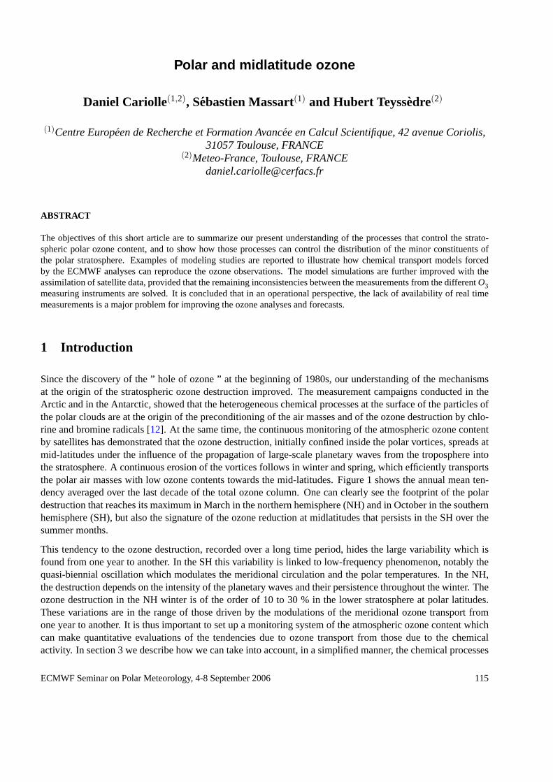
Since the discovery of the ” hole of ozone ” at the beginning of 1980s, our understanding of the mechanismsat the origin of the stratospheric ozone destruction improved. The measurement campaigns conducted in theArctic and in the Antarctic, showed that the heterogeneous chemical processes at the surface of the particles ofthe polar clouds are at the origin of the preconditioning of the air masses and of the ozone destruction by chlo-rine and bromine radicals [12]. At the same time, the continuous monitoring of the atmospheric ozone contentby satellites has demonstrated that the ozone destruction, initially confined inside the polar vortices, spreads atmid-latitudes under the influence of the propagation of large-scale planetary waves from the troposphere intothe stratosphere. A continuous erosion of the vortices follows in winter and spring, which efficiently transportsthe polar air masses with low ozone contents towards the mid-latitudes. Figure 1 shows the annual mean ten-dency averaged over the last decade of the total ozone column. One can clearly see the footprint of the polardestruction that reaches its maximum in March in the northern hemisphere (NH) and in October in the southernhemisphere (SH), but also the signature of the ozone reduction at midlatitudes that persists in the SH over thesummer months.

This tendency to the ozone destruction, recorded over a long time period, hides the large variability which isfound from one year to another. In the SH this variability is linked to low-frequency phenomenon, notably thequasi-biennial oscillation which modulates the meridional circulation and the polar temperatures. In the NH,the destruction depends on the intensity of the planetary waves and their persistence throughout the winter. Theozone destruction in the NH winter is of the order of 10 to 30 % in the lower stratosphere at polar latitudes.These variations are in the range of those driven by the modulations of the meridional ozone transport fromone year to another. It is thus important to set up a monitoring system of the atmospheric ozone content whichcan make quantitative evaluations of the tendencies due to ozone transport from those due to the chemicalactivity. In section 3 we describe how we can take into account, in a simplified manner, the chemical processes

ECMWF Seminar on Polar Meteorology, 4-8 September 2006 115

CARIOLLE, D. ET AL .: POLAR AND MIDLATITUDE OZONE

Figure 1: Ozone trend over the period 1978-2000 obtained from the analysis of TOMS and GOME data. Reprinted fromWMO2002 report [14]

controlling the ozone concentration in the general circulation models (GCMs), and how the assimilation of thesatellitedata can produce ozone fields showing a good consistency between transport and chemical processes.

2 Polar chemistry

The formation of the polar clouds is an essential element which determines the amplitude of the polar ozonedestruction in the stratosphere. In the SH, the polar vortex forms in the stratosphere in winter from June toSeptember. This vortex being relatively stable it remains centered over the pole, and the inside air masses coolgradually throughout the polar night. In spite of the very small humidities which prevail in the stratosphere, thetemperature falls enough so that nitric acid trihydrate (NAT) and ternary solutions ofHNO3, H2SO4, andH2O(STS) particles first form, followed by ice particles. In the lower stratosphere, it is considered that the NAT andSTS particles form below about 195K. Below 189 K, particles grow and are mainly composed of ice.

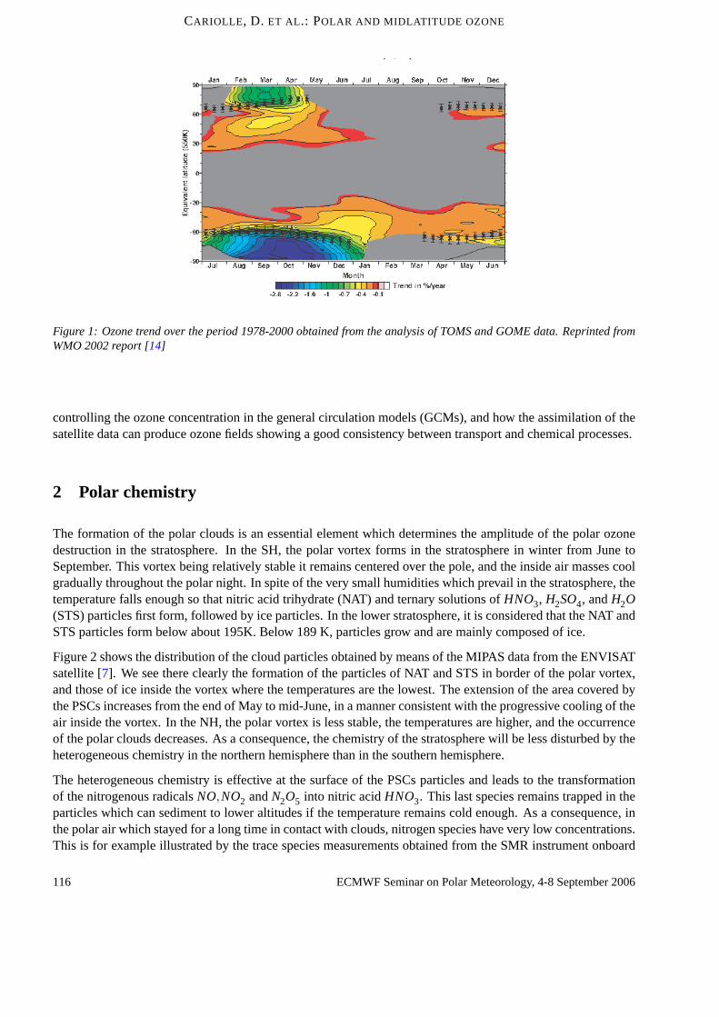
Figure 2 shows the distribution of the cloud particles obtained by means of the MIPAS data from the ENVISATsatellite [7]. We see there clearly the formation of the particles of NAT and STS in border of the polar vortex,andthose of ice inside the vortex where the temperatures are the lowest. The extension of the area covered bythe PSCs increases from the end of May to mid-June, in a manner consistent with the progressive cooling of theair inside the vortex. In the NH, the polar vortex is less stable, the temperatures are higher, and the occurrenceof the polar clouds decreases. As a consequence, the chemistry of the stratosphere will be less disturbed by theheterogeneous chemistry in the northern hemisphere than in the southern hemisphere.

The heterogeneous chemistry is effective at the surface of the PSCs particles and leads to the transformationof the nitrogenous radicalsNO,NO2 andN2O5 into nitric acidHNO3. This last species remains trapped in theparticles which can sediment to lower altitudes if the temperature remains cold enough. As a consequence, inthe polar air which stayed for a long time in contact with clouds, nitrogen species have very low concentrations.This is for example illustrated by the trace species measurements obtained from the SMR instrument onboard

116 ECMWF Seminar on Polar Meteorology, 4-8 September 2006


Figure 2: Distribution of PSC types at about 21 km derived from the MIPAS measurements over Antarctica during the2003summer. Red/orange are NAT particles, blue triangle are ice and blue-green circles are probably STS. Black dotsare PSC-free observations. The contour lines are based on the ECMWF temperature analyses and enclose the ice existingregion (blue), the STS region (green) and the NAT region(red). Reprinted from [7].

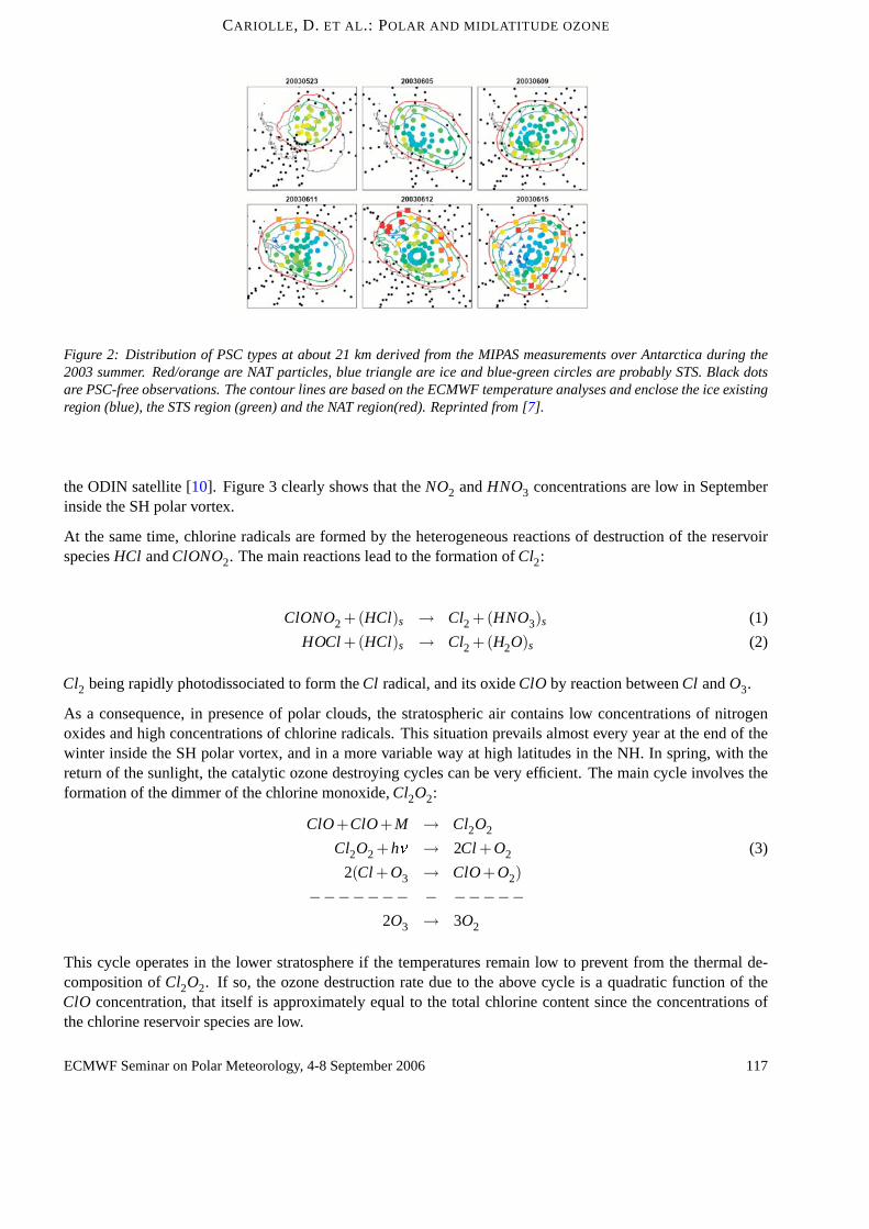
the ODIN satellite [10]. Figure 3 clearly shows that theNO2 andHNO3 concentrations are low in Septemberinside the SH polar vortex.

At the same time, chlorine radicals are formed by the heterogeneous reactions of destruction of the reservoirspeciesHCl andClONO2. The main reactions lead to the formation ofCl2:

ClONO2 +(HCl)s → Cl2 +(HNO3)s (1)

HOCl+(HCl)s → Cl2 +(H2O)s (2)

Cl2 beingrapidly photodissociated to form theCl radical, and its oxideClO by reaction betweenCl andO3.

As a consequence, in presence of polar clouds, the stratospheric air contains low concentrations of nitrogenoxides and high concentrations of chlorine radicals. This situation prevails almost every year at the end of thewinter inside the SH polar vortex, and in a more variable way at high latitudes in the NH. In spring, with thereturn of the sunlight, the catalytic ozone destroying cycles can be very efficient. The main cycle involves theformation of the dimmer of the chlorine monoxide,Cl2O2:

ClO+ClO+M → Cl2O2

Cl2O2 +hn → 2Cl +O2 (3)

2(Cl +O3 → ClO+O2)−−−−−−− − −−−−−

2O3 → 3O2

This cycle operates in the lower stratosphere if the temperatures remain low to prevent from the thermal de-composition ofCl2O2. If so, the ozone destruction rate due to the above cycle is a quadratic function of theClO concentration, that itself is approximately equal to the total chlorine content since the concentrations ofthe chlorine reservoir species are low.



Figure 3: Distribution of minor stratospheric trace species observed in the SH spring using the ODIN satellite. Courtesyof Ph. Ricaud [10].

In addition to the above cycle, the following catalytic cycle that involves the bromine species must be takeninto account:

BrO+ClO → Br +Cl +O2

→ BrCl +O2

BrCl +hn → Br +Cl (4)

Br +O3 → BrO+O2

Cl +O3 → ClO+O2

−−−−−− − −−−−−−2O3 → 3O2

Given the concentration of the current bromine loading in the stratosphere, the bromine cycle typically accountsfor about 30 % of the ozone destruction rate in the polar stratosphere. The above cycles can only be effectiveif the nitrogen oxide concentration is low, otherwiseClO will react withNO (reactionClO+NO→Cl +NO2)or with NO2 to formClONO2.

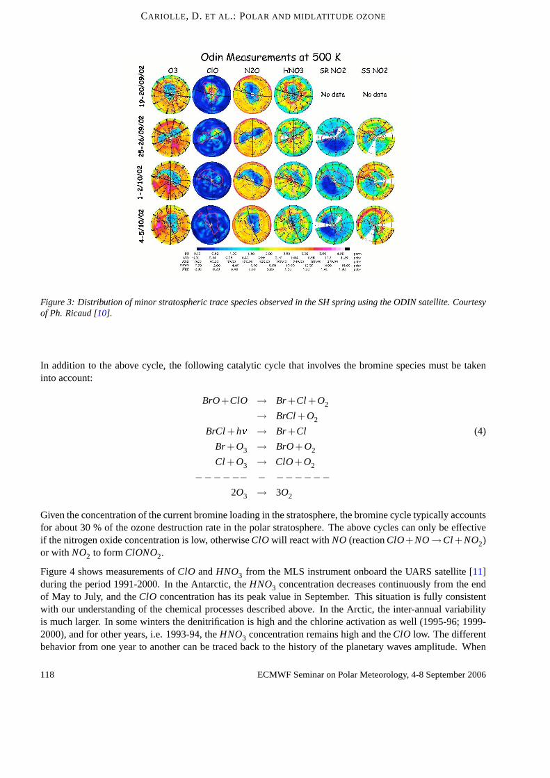
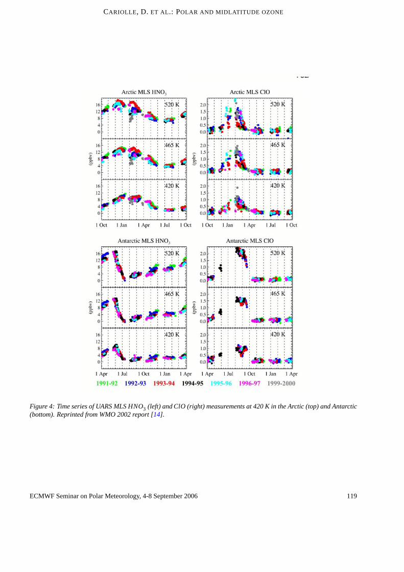
Figure 4 shows measurements ofClO andHNO3 from the MLS instrument onboard the UARS satellite [11]during the period 1991-2000. In the Antarctic, theHNO3 concentration decreases continuously from the endof May to July, and theClO concentration has its peak value in September. This situation is fully consistentwith our understanding of the chemical processes described above. In the Arctic, the inter-annual variabilityis much larger. In some winters the denitrification is high and the chlorine activation as well (1995-96; 1999-2000), and for other years, i.e. 1993-94, theHNO3 concentration remains high and theClO low. The differentbehavior from one year to another can be traced back to the history of the planetary waves amplitude. When



Figure 4: Time series of UARS MLS HNO3 (left) and ClO (right) measurements at 420 K in the Arctic (top) and Antarctic(bottom). Reprinted from WMO 2002 report [14].



the wave amplitude is low during most of the winter, the polar vortex remains cold, centered over the pole andsignificantozone destruction can occur in spring with the return of the sunlight. When the wave amplitude islarge, the polar temperatures are higher, the air masses are not processed by heterogeneous reactions and theozone destruction remains limited.

This variability in the planetary waves amplitude induces also large variations in the meridional ozone transport.In consequence, the evaluation of the net ozone destruction by chemistry is not easy. Recent evaluations,using chemical transport models (CTM), or based on analyses of the correlation between tracers and potentialvorticity distributions, show that about 10 to 30 % of the arctic ozone is depleted in winter-spring in the lowerstratosphere [14]. The next section discusses the prospects to improve those evaluations using chemical modelscoupledto assimilation of ozone data.

3 Modeling the polar and midlatitude ozone

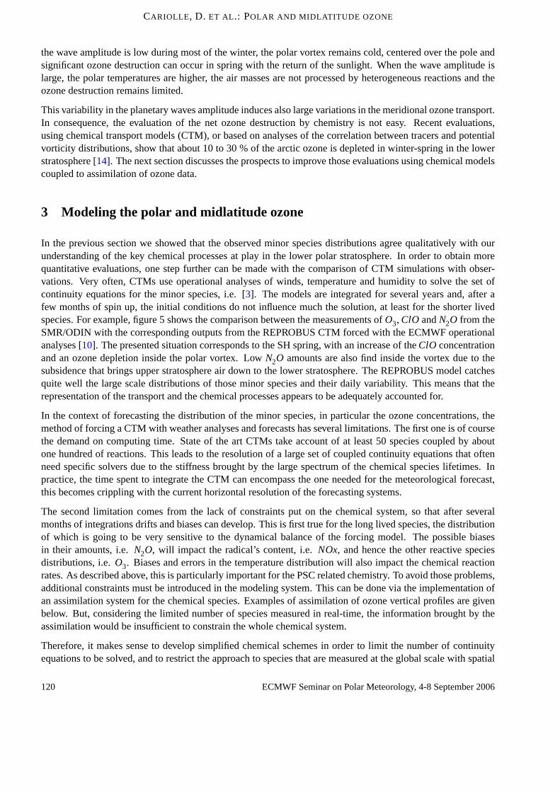
In the previous section we showed that the observed minor species distributions agree qualitatively with ourunderstanding of the key chemical processes at play in the lower polar stratosphere. In order to obtain morequantitative evaluations, one step further can be made with the comparison of CTM simulations with obser-vations. Very often, CTMs use operational analyses of winds, temperature and humidity to solve the set ofcontinuity equations for the minor species, i.e. [3]. The models are integrated for several years and, after afew months of spin up, the initial conditions do not influence much the solution, at least for the shorter livedspecies. For example, figure 5 shows the comparison between the measurements ofO3, ClO andN2O from theSMR/ODIN with the corresponding outputs from the REPROBUS CTM forced with the ECMWF operationalanalyses [10]. The presented situation corresponds to the SH spring, with an increase of theClO concentrationand an ozone depletion inside the polar vortex. LowN2O amounts are also find inside the vortex due to thesubsidence that brings upper stratosphere air down to the lower stratosphere. The REPROBUS model catchesquite well the large scale distributions of those minor species and their daily variability. This means that therepresentation of the transport and the chemical processes appears to be adequately accounted for.

In the context of forecasting the distribution of the minor species, in particular the ozone concentrations, themethod of forcing a CTM with weather analyses and forecasts has several limitations. The first one is of coursethe demand on computing time. State of the art CTMs take account of at least 50 species coupled by aboutone hundred of reactions. This leads to the resolution of a large set of coupled continuity equations that oftenneed specific solvers due to the stiffness brought by the large spectrum of the chemical species lifetimes. Inpractice, the time spent to integrate the CTM can encompass the one needed for the meteorological forecast,this becomes crippling with the current horizontal resolution of the forecasting systems.

The second limitation comes from the lack of constraints put on the chemical system, so that after severalmonths of integrations drifts and biases can develop. This is first true for the long lived species, the distributionof which is going to be very sensitive to the dynamical balance of the forcing model. The possible biasesin their amounts, i.e.N2O, will impact the radical’s content, i.e.NOx, and hence the other reactive speciesdistributions, i.e.O3. Biases and errors in the temperature distribution will also impact the chemical reactionrates. As described above, this is particularly important for the PSC related chemistry. To avoid those problems,additional constraints must be introduced in the modeling system. This can be done via the implementation ofan assimilation system for the chemical species. Examples of assimilation of ozone vertical profiles are givenbelow. But, considering the limited number of species measured in real-time, the information brought by theassimilation would be insufficient to constrain the whole chemical system.

Therefore, it makes sense to develop simplified chemical schemes in order to limit the number of continuityequations to be solved, and to restrict the approach to species that are measured at the global scale with spatial



Figure 5: Distribution of O3, ClO, and N2O observed in the SH spring using the ODIN satellite, and modelled for thesame dates by the REPROBUS chemical transport model. Courtesy of Ph. Ricaud [10].

and temporal resolutions coherent with those of the models. Such an approach is followed with the imple-mentationwithin the ARPEGE/Climat and the ECMWF IFS models of the linear ozone parameterization ofCariolle and Deque [1]. In that scheme the ozone continuity equation is expanded into Taylor series up to firstorderaround the local value of the ozone mixing ratio, the temperature and the overhead ozone column:

¶ rO3/¶ t = A1 +A2(rO3

−A3)+A4(T−A5)+A6(Σ−A7)+A8rO3(5)

where theAi termsare monthly averages calculated using the 2D photochemical model MOBIDIC:

A1 = (P−L) : Production and loss rate

A2 = ¶ (P−L)/¶ rO3

A3 = rO3: ozone mixing ratio

A4 = ¶ (P−L)/¶T

A5 = T : temperature

A6 = ¶ (P−L)/¶Σ

A7 = Σ : ozone column

A8: heterogeneous chemistry term,

whereas the other terms indicate the current 3D values of the ozone mixing ratiorO3, the temperature T, and the

local overhead ozone columnΣ, respectively.

The original scheme has been recently updated to account for PSC’s ozone chemistry [2], and is currently in



operation in the ECMWF IFS model since February 2006. One advantage of this scheme is its good stabilityandlack of drift in long term simulations due to the relaxation towards the climatology of the 2D model. [2]discussesthe CTM results when the linear scheme is used with forcing fields from the ECMWF operationalanalyses over the period 2000-2003. They found good agreement with Total Ozone Mapping Spectrometer(TOMS) data over that period, with a good representation by the model of the global distribution and theyear-to-year variability of the total ozone column.

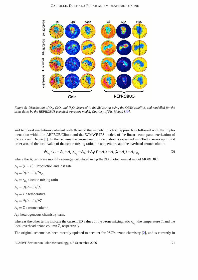
Figure 6: Time-latitude distributions of the total ozone column for two different years of a simulation of theARPEGE/Climatmodel forced by observed sea surface temperatures over the period 1990-1999.

The linear scheme has also been introduced in the version 2 of the ARPEGE/Climat model [4] and a 10 yearsimulationhas been performed with SST forcing from observations over the period 1990-1999. Figure 6 showsthe total ozone column modeled over two different years. For both years the observed characteristics of theclimatological ozone distribution are reproduced, with an equatorial minimum, spring maxima in the highnorthern latitudes, and a belt of high values around the polar minima in the SH in winter-spring. It is howeverinteresting to see that during the first year the final warming occurs quite early at the end of September andis associated with rather high ozone content in the polar vortex. Whereas during the second year, the polarvortex is more stable, and the ozone hole formed in September persists until the beginning of November. In theNH, the second year shows two pulses in the large amplitude waves associated to meridional ozone transport,



and the first one presents a steady situation with larger ozone content over the pole. Those results show that,despitethe simplicity of the linear scheme, free runs of the GCM give results as realistic as those of the CTMfor reproducing a large part of the ozone column variability.

With the perspective of producing accurate ozone analyses and forecasts the forced CTM simulations are valu-able, especially if the chemical system is introduced in a manner that prevent major biases and drifts. Thisappears to be the case with the linear model described above. However, it is anticipated that the model outputswould be further improved with the assimilation of ozone data.

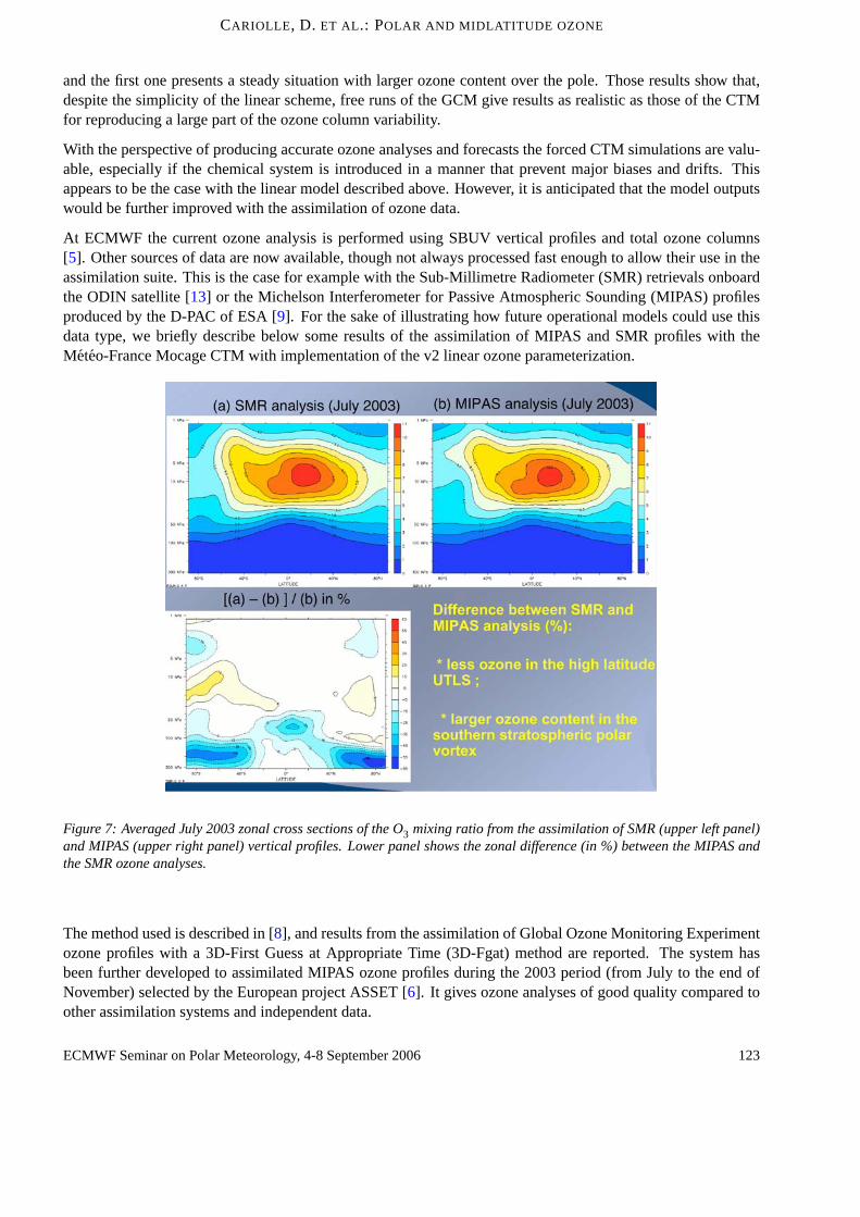
At ECMWF the current ozone analysis is performed using SBUV vertical profiles and total ozone columns[5]. Other sources of data are now available, though not always processed fast enough to allow their use in theassimilationsuite. This is the case for example with the Sub-Millimetre Radiometer (SMR) retrievals onboardthe ODIN satellite [13] or the Michelson Interferometer for Passive Atmospheric Sounding (MIPAS) profilesproducedby the D-PAC of ESA [9]. For the sake of illustrating how future operational models could use thisdatatype, we briefly describe below some results of the assimilation of MIPAS and SMR profiles with theMeteo-France Mocage CTM with implementation of the v2 linear ozone parameterization.

Figure 7: Averaged July 2003 zonal cross sections of the O3 mixingratio from the assimilation of SMR (upper left panel)and MIPAS (upper right panel) vertical profiles. Lower panel shows the zonal difference (in %) between the MIPAS andthe SMR ozone analyses.

The method used is described in [8], and results from the assimilation of Global Ozone Monitoring Experimentozoneprofiles with a 3D-First Guess at Appropriate Time (3D-Fgat) method are reported. The system hasbeen further developed to assimilated MIPAS ozone profiles during the 2003 period (from July to the end ofNovember) selected by the European project ASSET [6]. It gives ozone analyses of good quality compared tootherassimilation systems and independent data.



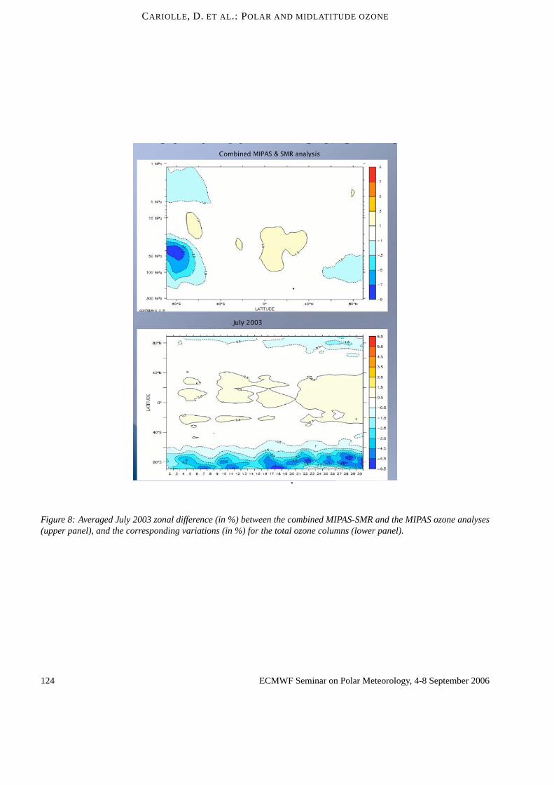
Figure 8: Averaged July 2003 zonal difference (in %) between the combined MIPAS-SMR and the MIPAS ozone analyses(upperpanel), and the corresponding variations (in %) for the total ozone columns (lower panel).



Our assimilation system has been further extended, the upper boundary of the model now reaches the 0.1 hPalevel, and the dynamical forcing comes from the operational IFS model. The assimilation can also cope withany instrument that gives vertical ozone profiles. Simulations have been performed using the MIPAS and theSMR data. Figure 7 shows the zonal mean cross sections of the stratospheric ozone for July 2003. At low andmid latitudes above 50 hPa the two assimilations give consistent results, with relative differences lower than5%. At polar southern latitudes the assimilation using the SMR data gives ozone contents that are higher by 5to 10 % compared to the MIPAS one above 40 hPa, but that are lower below that level.

In the upper troposphere lower stratosphere (UTLS), the MIPAS assimilation gives systematically higher valuesthan the SMR one. Since there is no SMR data assimilated below 70 hPa, it means that the MIPAS data drivethe model to a state where the ozone near the tropopause is much higher than the forced simulation withoutassimilation would produce. In the high northern latitude, the total ozone column produced by the MIPASassimilation is higher than the TOMS data by about 5%. At polar latitudes in the SH there is no data fromTOMS in July due to the polar night conditions and the comparison is not possible, but differences up to 8 %between TOMS and the MIPAS assimilation outputs are recorder later in the season. Thus, the high latitudeozone content produced by the MIPAS assimilation seems to be overestimated. Interestingly, the combinedassimilation of both datasets (Figure 8) correct a large part of the bias in the lower stratosphere, despite that thenumber of MIPAS profiles (about 1200/day) is much larger than the SMR profiles (about 300 profiles per day).The correction is the largest at southern polar latitudes, with ozone reductions that can reach 7% locally and4% for the total column.

4 Conclusion

In this paper we have discussed how chemical models can be validated against observations of the distributionof minor trace species. We conclude that current chemical transport models are able to take account of the mainprocesses that drive the polar ozone destruction, but due to limitations in the forcing fields, biases and driftscan develop during the course of the integrations.

Simplified models, using for example linearised schemes for chemical rates, introduce further constraints in thesystem that can limit those biases and prevent from major drifts. Since they are easy to implement, and use verylimited computer resources, they constitute a good choice for initial development of a forecasting system. Upto now, linear scheme are available for the computation of production and loss rates of ozone, but other speciesmay be considered in the future.

The assimilation of minor trace species observations introduce further constraints in the system, and shouldlead to improved forecasts. The results however will be dependent on the space and time densities of the obser-vations, and on the measurement errors. In the case of ozone, for which we have good quality measurements ofthe vertical distributions and the total columns, the combined analyses of the various datasets seem to be verypromising. However, not all those observations are available in real time, and therefore they cannot be used foroperational forecasting. They could however be used for re-analysis projects.

We have concentrated our discussions on the distribution of ozone in the stratosphere. In the tropospherethe situation would be more complex because of the difficulty to model transport processes in the boundarylayers, of the importance of liquid phase chemistry associated to clouds, and of the uncertainties in the ozoneprecursor emissions at ground level. In addition, observations of the distribution of minor trace species at theglobal scale, especially over the ocean, are available for a very limited number of species. This makes moredifficult the development and the assessment of the quality of assimilation suites.



References

[1] Cariolle, D. and Deque, M.: Southern hemisphere medium-scale waves and total ozone disturbances in aspectral general circulation model, J. Geophys. Res., 91, 10.825-10.846, 1986.

[2] Cariolle, D. and Teyssedre,H.: A revised linear ozone photochemistry parameterization for use in transportand general circulation models: Multi-annual simulations,Atmos. Chem. Phys., Submitted, acdp-0447, 2006.

[3] Chipperfield, M.: Multiannual simulations with a three-dimensional chemical transport model, J. Geophys.Res.,104,1781-1805, 1999.

[4] Deque,M., Dreveton, C., Braun, A. and Cariolle, D.: The ARPEGE/IFS atmosphere model: a contributionto the French community climate modelling, Climate Dynamics, 10, 249-266, 1994.

[5] Dethof, A. and Holm, E.: Ozone assimilation in the ERA-40 reanalysis project. Q. J. R. Meteorol. Soc.,131,2851-2872, 2004.

[6] Geer A. J., W. A. Lahoz, S. Bekki, N. Bormann, Q. Errera, H. J. Eskes, D. Fonteyn, D. R. Jackson, M.N.Juckes, S. Massart, V.-H. Peuch, S. Rharmili and A. Segers, The ASSET intercomparison of ozone analyses:method and first results, Atmos. Chem. Phys., submitted, 2006.

[7] Hopfner, M. , Larsen, N., Spang, R., Luo, B. P., Ma, J., Svendsen, S. H., Eckermann, S. D., Knudsen, B.,Massoli, P., Cairo, F., Stiller, G., Clarmann, T. v. and Fischer, H: MIPAS detects Antarctic stratospheric beltof NAT PSCs caused by mountain waves. Atmos. Chem. and Phys., Vol. 6, pp 1221-1230, 20-4-2006.

[8] Massart S., Cariolle D., Peuch V.-H. Vers une meilleure representationde la distribution et de la variabilitede l’ozone atmospherique par l’assimilation des donnees satellitaires. C.R. Acad. Sci., 337-15, 13051310,2005.

[9] Raspollini, P. , Belotti, C., Burgess, A., Carli, B., Carlotti, M., Ceccherini, S., Dinelli, B. M., Dudhia, A.,Flaud,J. -M., Funke, B., Hpfner, M., Lopez-Puertas, M., Payne, V., Piccolo, C., Remedios, J. J., Ridolfi, M.and Spang, R.: MIPAS level 2 operational analysis Atmos. Chem. and Phys. Disc., Vol. 6, pp 6525-6585,13-7-2006.

[10] Ricaud, P., Lefevre,F., Berthet, G., Murtagh, D., Llewellyn, E.,J., Megie, G., Kyrola, E., Leppelmeier,G. W., Auviven, H., Boonne, C., Brohede, S., Degenstein, D.A., de la Noe, J., Dupuy, E., El Amraoui, L.,Eriksson, P., Evans, W.F.J., Frisk, U., Gattinger, R.L., Girod, F., Haley, C.S., Hassinen, S., Hauchecorne,A., Jimenez, C., Kyro, E., Lautie, N., Le Flochmoen, E., Lloyd, N.D., McConnell, J.C., McDade, I.C.,Nordh, L., Olberg,M., Pazmino, A., Petelina, S.V., Sandqvist, A., Seppala, A., Sioris, B.H., Solheim, B.H.,Stegman, J., Strong, K., Taalas, P., Urban, J., von savigny, C., von Scheele, F., and Witt, G.: Polar vortexevolution during the 2002 Antarctic major warming as observed by the Odin satellite, J. Geophys. Res., 110,D05302, doi:10.1029/2004JD005018, 2005.

[11] Santee, M.L., G.L. Manney, N.J. Livesey, and J.W. Waters, UARS microwave Limb Sounder observationsof denitrification and ozone loss in the 2000 Arctic late winter. Geophys. Res. Lett., 27, 3213-3216, 2000.

[12] Solomon, S., 1999: Stratospheric ozone depletion: A review of concepts and history, Rev. Geophys., 37,275-316.

[13] Urban, J.; Lauti, N.; Le Flochmon, E.; Jimnez, C.; Eriksson, P.; d e La No, J.; Dupuy, E.; Ekstrm, M.; ElAmraoui,L.; Frisk, U.; Murtagh, D.; Olberg, M.; Ricaud, P.: Odin/SMR limb observations of stratospherictrace gases: Level 2 processing of ClO, N2O, HNO3, and O3. J. Geophys. Res., Vol. 110, No. D14, D14307,10.1029/2004JD005741,2005.



[14] WMO (World Meteorological Organization), Scientific Assessment of Ozone depletion: 2002, GlobalozoneResearch and Monitoring Project - Report No. 47, 498 pp., Geneva, 2003.

Acknowledgments

The authors would like to thank H. Fisher and J. Urban from providing material on the results from the MIPASand ODIN satellites that we have presented during the workshop.


Documents

Daniel Cariolle , Sebastien Massart´ and Hubert … · Daniel Cariolle(1,2), Sebastien Massart ... gradually throughout the polar night. In spite of the very small humidities which