Embed Size (px)
Citation preview
sensors
Article
Damage Identification in Various Types of CompositePlates Using Guided Waves Excited by a PiezoelectricTransducer and Measured by a Laser Vibrometer
Maciej Radzienski 1 , Paweł Kudela 1,* , Alessandro Marzani 2 , Luca De Marchi 3 andWiesław Ostachowicz 1
1 Institute of Fluid-Flow Machinery, Polish Academy of Sciences, 80-231 Gdansk, Poland;[email protected] (M.R.); [email protected] (W.O.)
2 Department of Civil, Chemical, Environmental and Materials Engineering, University of Bologna,40136 Bologna, Italy; [email protected]
3 Department of Electrical, Electronic, and Information Engineering, University of Bologna, 40136 Bologna,Italy; [email protected]
* Correspondence: [email protected]
Received: 11 April 2019; Accepted: 25 April 2019; Published: 26 April 2019�����������������
Abstract: Composite materials are widely used in the industry, and the interest of this material isgrowing rapidly, due to its light weight, strength and various other desired mechanical properties.However, composite materials are prone to production defects and other defects originated duringexploitation, which may jeopardize the safety of such a structure. Thus, non-destructive evaluationmethods that are material-independent and suitable for a wide range of defects identification areneeded. In this paper, a technique for damage characterization in composite plates is proposed. In thepresented non-destructive testing method, guided waves are excited by a piezoelectric transducer,attached to tested specimens, and measured by a scanning laser Doppler vibrometer in a densegrid of points. By means of signal processing, irregularities in wavefield images caused by anymaterial defects are extracted and used for damage characterization. The effectiveness of theproposed technique is validated on four different composite panels: Carbon fiber-reinforced polymer,glass fiber-reinforced polymer, composite reinforced by randomly-oriented short glass fibers andaluminum-honeycomb core sandwich composite. Obtained results confirm its versatility and efficacyin damage characterization in various types of composite plates.
Keywords: laser vibrometry; SLDV; guided waves; damage detection; NDT; full wavefield processing
1. Introduction
Guided Waves (GW) have received considerable attention in recent years, as a tool for damagedetection and localization in both Structural Health Monitoring (SHM) systems and Non-DestructiveTesting (NDT).
In the SHM system, typically an array of piezoelectric transducers (PZTs) is used for excitationand sensing. Various configurations may be found in the literature [1–4], and can be divided into twomain groups: Pulse echo [5] and pitch-catch [6]. Algorithms for damage localization often utilizegroup velocities [7] of propagating Lamb wave modes, dispersion curves of particular wave mode [5]or full waveform inversion [8]. Alternatively, the time reversal approach is used [9,10]. The review ofGW-based SHM strategies was presented by Mitra and Gopalakrishnan [11].
The advantage of such a system is the ability of permanent integration and online monitoringof changes in GW propagation in structural elements. The main problem of application of the arrayconsisting of a few PZTs for damage localization, is that the damage imaging resolution can be quite
Sensors 2019, 19, 1958; doi:10.3390/s19091958 www.mdpi.com/journal/sensors

Sensors 2019, 19, 1958 2 of 17
low. On the other hand, the application of a very dense array of PZTs is not feasible. This problem canbe alleviated by using scanning laser Doppler vibrometry.
Scanning laser vibrometry allows for measurement of guided waves in a dense grid of pointsacross the surface of a large specimen [12]. Such a collection of signals is often called full wavefield.However, it should be noticed, that the measurement process can be time-consuming. Therefore,such a technique can be classified as NDT instead of SHM. Nevertheless, laser and optics technologyprogresses very fast, so it is expected that multipoint vibrometers, fast cameras, etc. may be used in thefuture for full wavefield measurements.
Anomalies of GW propagating in honeycomb core sandwich plates with debonding were studiednumerically, as well as by using laser vibrometer data by Zhao et al. [13]. Various techniques of damagelocalization were developed in recent years using various phenomena like wave reflection detection [14],local standing wave [15], a local change in wavelength [16], energy distribution variations [17,18],local magnitude decrease [19], etc. GW measurement techniques, along with full wavefield processingtechniques for damage detection, were summarized in the paper [20]. Usually, single PZT is used forGW excitation, but also high power laser can be used for pulsed excitation of thermo-elastic waves,which in conjunction with the laser vibrometer, leads to a complete non-contact monitoring system [21].
The aim of this research is the development of a versatile and robust technique for mappinganomalies in guided waves in plate-like structures, regardless of material properties. The proposedmethod can be used for various hidden defects visualization without any prior knowledge abouttested material properties or its reference state (measurement data for the undamaged case). It givesthe greatest flexibility of application among full wavefield techniques available in the literature.
The paper is organized as follows: The steps of the proposed method for hidden defectsvisualization are given in Section 2, followed by experimental results carried out on specimens madeout of carbon fiber reinforced polymer (CFRP), glass fiber reinforced polymer (GFRP), randomlyoriented short fiber reinforced polymer (SFRP) and honeycomb sandwich panel (HCSP). The resultsare briefly discussed in Section 4.
2. Method for Detection of Anomalies in Guided Wave Propagation
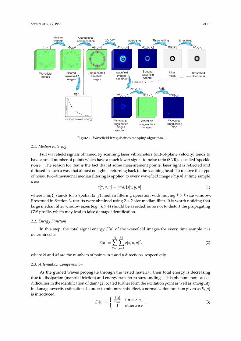
The method proposed in this research approach is based on the filtering technique in wavenumberdomain originally proposed in [22] for identification of cracks in the plate-like structure, which waslater modified for impact-induced damage detection by Kudela et al. [23]. The method is furtherexpanded in this paper for the identification of any anomalies in propagating GW in a broad rangeof isotropic and anisotropic structures. The modification allows for a greater range of applicabilityof the proposed damage identification algorithm. Mapping irregularities in propagating GW maybe used as a tool for any material local changes characterization (e.g., fatigue crack, delamination,debonding), without any prior knowledge about material properties or its reference state. It is amulti-step process. Each step of the algorithm is schematically presented in Figure 1. All the stepsare indicated by arrows with consecutive numbers, and the corresponding description of each step ispresented in the next sections.
Sensors 2019, 19, 1958 3 of 17
Sensors 2019, 19, x FOR PEER REVIEW 3 of 17
Figure 1. Wavefield irregularities mapping algorithm.
2.1. Median Filtering
Full wavefield signals obtained by scanning laser vibrometers (out-of-plane velocity) tends to
have a small number of points which have a much lower signal-to-noise ratio (SNR), so-called
‘speckle noise’. The reason for that is the fact that at some measurement points, laser light is reflected
and diffused in such a way that almost no light is returning back to the scanning head. To remove
this type of noise, two-dimensional median filtering is applied to every wavefield image s[x,y,n] at
time sample n as:
𝑣[𝑥, 𝑦, 𝑛] = 𝑚𝑒𝑑𝑘{𝑠[𝑥, 𝑦, 𝑛]}, (1)
where medk{} stands for a spatial (x, y) median filtering operation with moving k × k size window.
Presented in Section 3, results were obtained using 2 × 2 size median filter. It is worth noticing that
large median filter window sizes (e.g., k > 4) should be avoided, so as not to distort the propagating
GW profile, which may lead to false damage identification.
2.2. Energy Function
In this step, the total signal energy E[n] of the wavefield images for every time sample n is
determined as:
𝐸[𝑛] = ∑ ∑ 𝑣[𝑥, 𝑦, 𝑛]2
𝑀
𝑦=1
,
𝑁
𝑥=1
(2)
where N and M are the numbers of points in x and y directions, respectively.
2.3. Attenuation Compensation
As the guided waves propagate through the tested material, their total energy is decreasing due
to dissipation (material friction) and energy transfer to surroundings. This phenomenon causes
difficulties in the identification of damage located further form the excitation point as well as
ambiguity in damage severity estimation. In order to minimize this effect, a normalization function
given as Er[n] is introduced:
Figure 1. Wavefield irregularities mapping algorithm.
2.1. Median Filtering
Full wavefield signals obtained by scanning laser vibrometers (out-of-plane velocity) tends tohave a small number of points which have a much lower signal-to-noise ratio (SNR), so-called ‘specklenoise’. The reason for that is the fact that at some measurement points, laser light is reflected anddiffused in such a way that almost no light is returning back to the scanning head. To remove this typeof noise, two-dimensional median filtering is applied to every wavefield image s[x,y,n] at time samplen as:
v[x, y, n] = medk{s[x, y, n]
}, (1)
where medk{} stands for a spatial (x, y) median filtering operation with moving k × k size window.Presented in Section 3, results were obtained using 2 × 2 size median filter. It is worth noticing thatlarge median filter window sizes (e.g., k > 4) should be avoided, so as not to distort the propagatingGW profile, which may lead to false damage identification.
2.2. Energy Function
In this step, the total signal energy E[n] of the wavefield images for every time sample n isdetermined as:
E[n] =N∑
x=1
M∑y=1
v[x, y, n]2, (2)
where N and M are the numbers of points in x and y directions, respectively.
2.3. Attenuation Compensation
As the guided waves propagate through the tested material, their total energy is decreasingdue to dissipation (material friction) and energy transfer to surroundings. This phenomenon causesdifficulties in the identification of damage located further form the excitation point as well as ambiguityin damage severity estimation. In order to minimize this effect, a normalization function given as Er[n]is introduced:
Er[n] =
E[n]Emax
for n ≥ na
1 otherwise. (3)

Sensors 2019, 19, 1958 4 of 17
where Emax = max(E[n]). The normalization is applied to the full wavefield, so that guided fullwavefield signal with compensated attenuation w[x,y,n], is obtained
w[x, y, n] =v[x, y, n]
Er[n]. (4)
The exemplary normalization function Er is presented in Figure 2 (grey dashed line).
Sensors 2019, 19, x FOR PEER REVIEW 4 of 17
𝐸𝑟[𝑛] = {
𝐸[𝑛]
𝐸𝑚𝑎𝑥 for 𝑛 ≥ 𝑛𝑎
1 otherwise
. (3)
where Emax = max(E[n]). The normalization is applied to the full wavefield, so that guided full
wavefield signal with compensated attenuation w[x,y,n], is obtained
𝑤[𝑥, 𝑦, 𝑛] =𝑣[𝑥, 𝑦, 𝑛]
𝐸𝑟[𝑛]. (4)
The exemplary normalization function Er is presented in Figure 2 (grey dashed line).
Figure 2. Normalized Guided Waves (GW) energy function E/Emax and attenuation compensation
function Er.
Normalized to unity energy function E/Emax (Figure 2—black line) is also used to define the time
interval between time sample na (Figure 2—blue dashed line), when the signal has maximum energy,
and nb (Figure 2—red dashed line), when its energy drops to a given threshold (e.g., 10%). This
interval is regarded as most advantageous for wavefield irregularities mapping, and it is used further
in Equation 16.
2.4. Two-Dimensional Discrete Fourier Transform
All wavefield images are transformed from the space-space-time domain into a wavenumber-
wavenumber-time domain by two-dimensional discrete Fourier transform (2D DFT)
𝑊[𝑘𝑥, 𝑘𝑦, 𝑛] =1
√𝑀𝑁∑ ∑ 𝑣[𝑥, 𝑦, 𝑛] ∙ 𝑒
−𝑖2𝜋(𝑘𝑥𝑥
𝑁+
𝑘𝑦𝑦
𝑀 ),
𝑀
𝑦=1
𝑁
𝑥=1
𝑛 ∈ ℕ: ⟨1, 𝑃⟩, (5)
where kx and ky are wavenumbers in the x and y directions, respectively. 2D DFT is applied for each
time frame-wavefield image, therefore P transformations are performed, were P is the number of
wavefield images (number of registered time samples in each point).
2.5. Spectral Wavefield Pattern
In wavenumber domain a spectral wavefield pattern is determined through averaging a set of
wavefield images in the time interval between nc and nd:
𝑊𝑎𝑣𝑔[𝑘𝑥, 𝑘𝑦] =1
𝑛𝑑 − 𝑛𝑐∑ 𝑊[𝑘𝑥, 𝑘𝑦, 𝑛],
𝑛𝑑
𝑛=𝑛𝑐
(6)
Figure 2. Normalized Guided Waves (GW) energy function E/Emax and attenuation compensationfunction Er.
Normalized to unity energy function E/Emax (Figure 2—black line) is also used to define the timeinterval between time sample na (Figure 2—blue dashed line), when the signal has maximum energy,and nb (Figure 2—red dashed line), when its energy drops to a given threshold (e.g., 10%). Thisinterval is regarded as most advantageous for wavefield irregularities mapping, and it is used furtherin Equation 16.
2.4. Two-Dimensional Discrete Fourier Transform
All wavefield images are transformed from the space-space-time domain into awavenumber-wavenumber-time domain by two-dimensional discrete Fourier transform (2D DFT)
W[kx, ky, n
]=
1√
MN
N∑x=1
M∑y=1
v[x, y, n]·e−i2π( kxxN +
ky yM ), n ∈ N : 〈1, P〉, (5)
where kx and ky are wavenumbers in the x and y directions, respectively. 2D DFT is applied for eachtime frame-wavefield image, therefore P transformations are performed, were P is the number ofwavefield images (number of registered time samples in each point).
2.5. Spectral Wavefield Pattern
In wavenumber domain a spectral wavefield pattern is determined through averaging a set ofwavefield images in the time interval between nc and nd:
Wavg[kx, ky
]=
1nd − nc
nd∑n=nc
W[kx, ky, n
], (6)

Sensors 2019, 19, 1958 5 of 17
where nc and nd are determined as:nc = na − n f , (7)
nd = nb + n f . (8)
Value of nf is chosen to meet the conditions:
E[na − n f
]Emax
≈ 0.5n f ∈ N : n f < na. (9)
The exemplary E/Emax function with na, nc and nd position marked are presented in Figure 3.
Sensors 2019, 19, x FOR PEER REVIEW 5 of 17
where nc and nd are determined as:
𝑛𝑐 = 𝑛𝑎 − 𝑛𝑓, (7)
𝑛𝑑 = 𝑛𝑏 + 𝑛𝑓. (8)
Value of nf is chosen to meet the conditions:
𝐸[𝑛𝑎 − 𝑛𝑓]
𝐸𝑚𝑎𝑥≈ 0.5 𝑛𝑓 ∈ ℕ: 𝑛𝑓 < 𝑛𝑎. (9)
The exemplary E/Emax function with na, nc and nd position marked are presented in Figure 3.
2.6. Filter Mask
Based on the spectral wavefield pattern a filter mask M is determined as:
𝑀[𝑘𝑥, 𝑘𝑦] = {0 𝑖𝑓 𝑊𝑎𝑣𝑔(𝑘𝑥, 𝑘𝑦) > threshold
1 otherwise . (10)
The threshold is chosen to be the 95th percentile of Wavg values. It may be determined by finding the
Wavg value for which its cumulative distribution function reaches 0.95. If the threshold will be too high
(not enough points will be filtered), some portion of the regular wave propagation component will
not be filtered, thus making final irregularities map to have high values across the whole inspected
region. On the other hand, setting threshold too low (too many points will be filtered) will result in
blurred irregularities mapping up to the point that they are removed from the signal completely.
However, even a wide range of threshold values around the 95th percentile of Wavg values will give
good results.
Figure 3. Normalized GW energy function E/Emax with marked by blue and red dashed line time
interval used for wavefield pattern estimation.
2.7. Smoothing Filter Mask
A rotationally symmetric Gaussian low pass filter G is used to smooth filter mask M throughout
the convolution operation
��[𝑘𝑥, 𝑘𝑦] = 𝑀[𝑘𝑥, 𝑘𝑦] ∗ 𝐺[𝑘𝑥, 𝑘𝑦]. (11)
The standard deviation σ and size of the filter may be chosen from a wide range of values. In this
study σ = 2 and 10 × 10 points size G were used.
Figure 3. Normalized GW energy function E/Emax with marked by blue and red dashed line timeinterval used for wavefield pattern estimation.
2.6. Filter Mask
Based on the spectral wavefield pattern a filter mask M is determined as:
M[kx, ky
]=
0 i f Wavg(kx, ky
)> threshold
1 otherwise. (10)
The threshold is chosen to be the 95th percentile of Wavg values. It may be determined by finding theWavg value for which its cumulative distribution function reaches 0.95. If the threshold will be too high(not enough points will be filtered), some portion of the regular wave propagation component will notbe filtered, thus making final irregularities map to have high values across the whole inspected region.On the other hand, setting threshold too low (too many points will be filtered) will result in blurredirregularities mapping up to the point that they are removed from the signal completely. However,even a wide range of threshold values around the 95th percentile of Wavg values will give good results.
2.7. Smoothing Filter Mask
A rotationally symmetric Gaussian low pass filter G is used to smooth filter mask M throughoutthe convolution operation
M[kx, ky
]= M
[kx, ky
]∗G
[kx, ky
]. (11)

Sensors 2019, 19, 1958 6 of 17
The standard deviation σ and size of the filter may be chosen from a wide range of values. In this studyσ = 2 and 10 × 10 points size G were used.
G[kx, ky
]=
g[kx, ky
]∑
kx
∑ky g
[kx, ky
] , (12)
where
g[kx, ky
]= e
−(kx2+ky2)
2σ2 . (13)
2.8. Filtering
A designated smoothed filter mask M is successively used for the elimination of main wavefieldcomponents in every wavefield image in the wavenumber domain by element-wise multiplication as:
W[kx, ky, n
]= W
[kx, ky, n
]◦ M
[kx, ky
], n ∈ N : 〈1, P〉. (14)
This operation removes the regular component of GW, leaving an irregular component of wavefieldimages caused by abnormalities in GW-like local changes in wavelength, amplitude, wavefrontorientation, or the occurrence of reflection.
2.9. Inverse Two-Dimensional Discrete Fourier Transform
To transform the wavefield irregularities images from the wavenumber-wavenumber-time domainback into the space-space-time domain, an inverse two-dimensional discrete Fourier transform (Inv.2D DFT) is applied for each wavefield image (time frame) as:
w[x, y, n] =1√
MN
N∑kx=1
M∑ky=1
W[kx, ky, n
]·ei2π( kxx
N +ky yM ), n ∈ N : 〈1, P〉. (15)
2.10. Root Mean Squared
In step 9, a series of processed images for consecutive time moments are obtained. To fuseinformation about any abnormality in wavefield images into a single map, the Root Mean Squared(RMS) function is used. The final wavefield irregularities map is given as follows:
IRM[x, y] =
√√√1
nb − na
nb∑n=na
(w[x, y, n])2. (16)
3. Experimental Verification
3.1. Experimental Set-Up
In each tested specimen (detailed description in Section 3.2), guided waves were excited by around piezoelectric transducer (Sonox® P502 produced by CeramTec) of a 10 mm diameter. Accordingto the producer datasheet, its thickness resonance is 3.8 MHz, and the planar resonance is 203 kHz.The transducer was attached by an acrylic glue (Kropelka® made in Uruguay) to the back surfaceof each investigated specimen in its geometrical center. The signal in a form of 5 sine cycles with50 kHz frequency modulated by Hann window was generated by an arbitrary waveform generator(Aim & Thurlby Thandar Instruments TGA 1241), and amplified to 200 Vpp by a Linear Amplifier(Piezosystems EPA-104). Guided waves were measured by a scanning laser Doppler vibrometer(Polytec PSV-400) as out-of-plane velocities in a regular grid of 251 × 251 points covering the wholefront surface of investigated specimens. The scheme of the experimental set-up is presented in Figure 4.

Sensors 2019, 19, 1958 7 of 17
Sensors 2019, 19, x FOR PEER REVIEW 7 of 17
Measurements were performed in point by point manner, and were synchronized with
excitation. Between each excitation 10 ms delay was used to ensure that all previously excited GW
attenuated. In each measuring point, 512 time samples were registered with a 512 kHz sampling rate,
which gives a total of 1 ms measured time response. Every signal was measured 10 times, and the
averaged value was designed to improve signal quality. Full wavefield measurements took 6 h for
each investigated specimen.
Figure 4. Experimental set-up.
3.2. Specimens
In order to verify the proposed wavefield irregularities mapping technique for damage
identification, four various composite plates, namely: CFRP, GFRP, SFRP, HCSP specimens with
various defects were investigated. A detailed description of specimens is given in Subsections 3.2.1–
3.2.4, and the schemes are presented in Figure 5.
All tested specimens front surfaces were covered with retro-reflective tape in order to increase
the SNR of measured time responses. All specimens were of 500 mm width, and 500 mm length and,
various thickness. Specimens were hung by a tiny string attached to its sides to reduce the external
influences and simulate free-free conditions.
3.2.1. CFRP
Carbon fiber reinforced polymer plate consists of 16 woven fabric layers (GG204P-IMP503 pre-
pregs) with fibers orienting 0° and 90° in every layer. The total thickness of the specimen is 3 mm. A
15 × 15 mm square Teflon insert was introduced to the sample during the manufacturing process
between layers 8 and 9 to simulate a delamination. The scheme of the sample with the delamination
position is presented in Figure 5a.
3.2.2. GFRP
Glass fiber reinforced polymer plate consists of 12 woven fabric layers (GG204P-VV192T/202
pre-pregs) with fiber orienting 0° and 90° in every layer. The total thickness of the specimen is 2 mm.
Four round Teflon inserts with a diameter of 20 mm were introduced to the sample during the
manufacturing process. Positions of the delaminations in thickness are given in Table 1 and presented
in Figure 5b.
Table 1. Positions of Teflon inserts in glass fiber reinforced polymer (GFRP) specimen.
Designation Position in Thickness Size
D1 between 10th and 9th layer d = 20 mm
D2 between 8th and 7th layer d = 20 mm
D3 between 6th and 5th layer d = 20 mm
Figure 4. Experimental set-up.
Measurements were performed in point by point manner, and were synchronized with excitation.Between each excitation 10 ms delay was used to ensure that all previously excited GW attenuated.In each measuring point, 512 time samples were registered with a 512 kHz sampling rate, whichgives a total of 1 ms measured time response. Every signal was measured 10 times, and the averagedvalue was designed to improve signal quality. Full wavefield measurements took 6 h for eachinvestigated specimen.
3.2. Specimens
In order to verify the proposed wavefield irregularities mapping technique for damageidentification, four various composite plates, namely: CFRP, GFRP, SFRP, HCSP specimens withvarious defects were investigated. A detailed description of specimens is given in Sections 3.2.1–3.2.4,and the schemes are presented in Figure 5.
All tested specimens front surfaces were covered with retro-reflective tape in order to increasethe SNR of measured time responses. All specimens were of 500 mm width, and 500 mm length and,various thickness. Specimens were hung by a tiny string attached to its sides to reduce the externalinfluences and simulate free-free conditions.
3.2.1. CFRP
Carbon fiber reinforced polymer plate consists of 16 woven fabric layers (GG204P-IMP503pre-pregs) with fibers orienting 0◦ and 90◦ in every layer. The total thickness of the specimen is 3 mm.A 15 × 15 mm square Teflon insert was introduced to the sample during the manufacturing processbetween layers 8 and 9 to simulate a delamination. The scheme of the sample with the delaminationposition is presented in Figure 5a.
3.2.2. GFRP
Glass fiber reinforced polymer plate consists of 12 woven fabric layers (GG204P-VV192T/202pre-pregs) with fiber orienting 0◦ and 90◦ in every layer. The total thickness of the specimen is2 mm. Four round Teflon inserts with a diameter of 20 mm were introduced to the sample during themanufacturing process. Positions of the delaminations in thickness are given in Table 1 and presentedin Figure 5b.
Table 1. Positions of Teflon inserts in glass fiber reinforced polymer (GFRP) specimen.
Designation Position in Thickness Size
D1 between 10th and 9th layer d = 20 mmD2 between 8th and 7th layer d = 20 mmD3 between 6th and 5th layer d = 20 mmD4 between 4th and 3rd layer d = 20 mm

Sensors 2019, 19, 1958 8 of 17
Sensors 2019, 19, x FOR PEER REVIEW 8 of 17
3.2.3. SFRP
Randomly-oriented short fiber-reinforced polymer plate comprises 4 mm long glass fiber
bundles (40% by weight) evenly distributed in epoxy resin (Ampreg 22). The sample has a uniform
thickness of 3 mm. In this specimen, the damage was prepared as a 20 × 20 mm area of reduced
thickness by 50% from the back side. The scheme of the sample with damage position is presented in
Figure 5c.
3.2.4. HCSP
Honeycomb sandwich panel is composed of two 1 mm thick 5005 aluminum sheets and 5 mm
tall aluminum honeycomb core (3003 aluminum foil of 50 microns thickness and 12 mm cells
diameter) bonded in between. In the central part of the specimen, during the manufacturing process,
the aluminum core was crushed at the area of about 125 × 125 mm. Additionally, two regions where
the inner core was disbonded from the outer layer were introduced. The scheme of the HCSP
specimen with its deteriorated areas is presented in Figure 5d.
(a)
(b)
(c)
(d)
Figure 5. Specimens with defects schemes: (a) Carbon fiber reinforced polymer (CFRP); (b) glassfiber reinforced polymer (GFRP); (c) randomly oriented short fiber reinforced polymer (SFRP) and (d);honeycomb sandwich panel (HCSP).
3.2.3. SFRP
Randomly-oriented short fiber-reinforced polymer plate comprises 4 mm long glass fiber bundles(40% by weight) evenly distributed in epoxy resin (Ampreg 22). The sample has a uniform thickness of3 mm. In this specimen, the damage was prepared as a 20 × 20 mm area of reduced thickness by 50%from the back side. The scheme of the sample with damage position is presented in Figure 5c.
3.2.4. HCSP
Honeycomb sandwich panel is composed of two 1 mm thick 5005 aluminum sheets and 5 mm tallaluminum honeycomb core (3003 aluminum foil of 50 microns thickness and 12 mm cells diameter)bonded in between. In the central part of the specimen, during the manufacturing process, thealuminum core was crushed at the area of about 125 × 125 mm. Additionally, two regions where theinner core was disbonded from the outer layer were introduced. The scheme of the HCSP specimenwith its deteriorated areas is presented in Figure 5d.
Sensors 2019, 19, 1958 9 of 17
3.3. Results
3.3.1. Wavefield Images
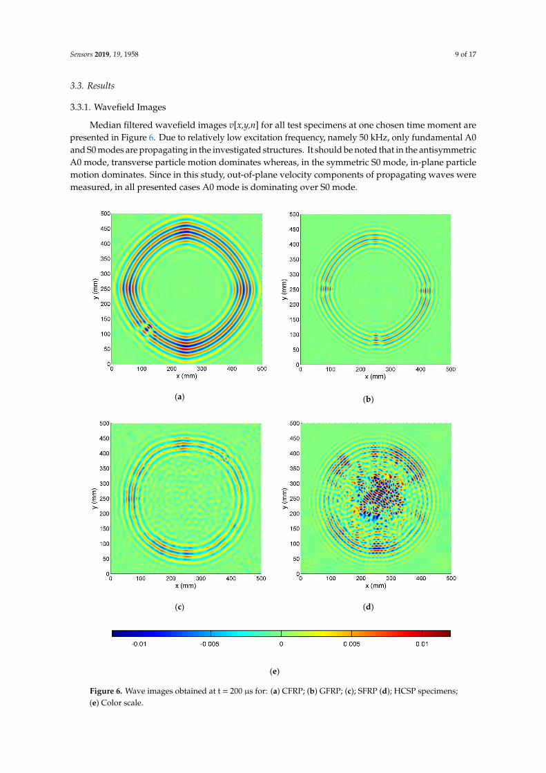
Median filtered wavefield images v[x,y,n] for all test specimens at one chosen time moment arepresented in Figure 6. Due to relatively low excitation frequency, namely 50 kHz, only fundamental A0and S0 modes are propagating in the investigated structures. It should be noted that in the antisymmetricA0 mode, transverse particle motion dominates whereas, in the symmetric S0 mode, in-plane particlemotion dominates. Since in this study, out-of-plane velocity components of propagating waves weremeasured, in all presented cases A0 mode is dominating over S0 mode.
Sensors 2019, 19, x FOR PEER REVIEW 9 of 17
Figure 5. Specimens with defects schemes: (a) Carbon fiber reinforced polymer (CFRP); (b) glass fiber
reinforced polymer (GFRP); (c) randomly oriented short fiber reinforced polymer (SFRP) and (d);
honeycomb sandwich panel (HCSP).
3.3. Results
3.3.1. Wavefield Images
(a)
(b)
(c)
(d)
(e)
Figure 6. Wave images obtained at t = 200 µs for: (a) CFRP; (b) GFRP; (c); SFRP (d); HCSP specimens;
(e) Color scale.
Figure 6. Wave images obtained at t = 200 µs for: (a) CFRP; (b) GFRP; (c); SFRP (d); HCSP specimens;(e) Color scale.

Sensors 2019, 19, 1958 10 of 17
In Figure 6a (CFRP specimen) wavefront of propagating GW is smooth and elongated in thehorizontal and vertical direction, which corresponds to fibers orientation. The occurrence of damage isvisible in the left bottom quarter of the image as a local disturbance of wavelength and amplitude.
In Figure 6b (GFRP specimen) wavefront is almost circular with evident distortions at fourquadrants, where the delaminations are located. Also reflected from Teflon inserts, small amplitudewaves may be noticed inside the circular shape. The smallest changes in wavefront are visible in thetop quadrant (delamination D1) where the Teflon insert is located farthest from the measured surface.
In Figure 6c (SFRP specimen) wavefront is rugged both in terms of wave position (related towave velocity) and amplitude. Small amplitude GW reflections are spread across the whole specimensurface. Therefore, damage position (top-right quarter) is hard to be distinguished.
In Figure 6d (HCSP specimen) the circular wavefront has a strong variation in the amplitudealong its circumference. High amplitude wave reflections occur in the specimen’s center part wherethe crushed core area is located.
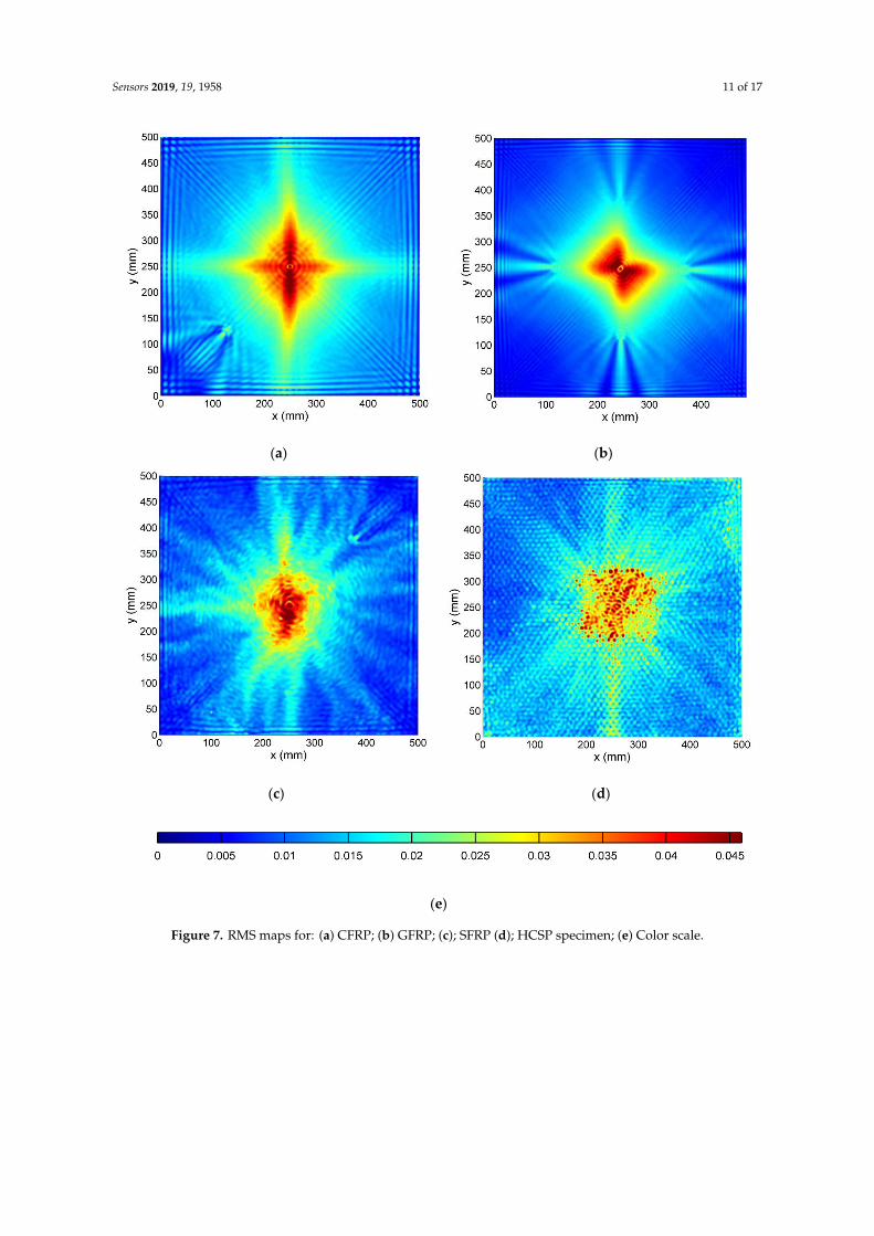
RMS maps of tested specimens calculated for median-filtered registered full wavefield signalsv[x,y,n] are presented in Figure 7. Due to high GW attenuation in tested materials, most of the energyof the wave is concentrated around the excitation point. For comparison purposes also, RMS mapsdetermined for compensated signals w[x,y,n], are presented in Figure 8.
In the CFRP sample (Figure 7a) energy of GW is spread more in fibers directions, creating across-like shape in the center. This phenomenon is less apparent in GFRP specimen (Figure 7b), wherebesides this effect also, energy is distributed more in the direction of two corners (top-left corner andbottom-right corner). This is most probably caused by asymmetry in the PZT transducer, which hasone of the electrodes wrapped around from the bottom to the top surface.
It is worth it to notice that all Teflon inserts (CFRP and GFRP specimens) create similar patterns inRMS maps. Higher amplitude beams are formed behind delaminations in a straight line for excitationpoint, and some small side lobes on both its sides are separated by lower value regions.
For SFRP specimen, RMS map (Figure 7c) is much more scattered, and damage position is muchless evident, but it is creating a similar pattern to the case of delaminations.
The crushed core region of HCSP appears as a high-value area in the RMS map (Figure 7d). Frontplate disbonding has a small increase in RMS amplitude, and back plate disbonding manifests itself aslower amplitude area.
Sensors 2019, 19, 1958 11 of 17
Sensors 2019, 19, x FOR PEER REVIEW 10 of 17
Median filtered wavefield images v[x,y,n] for all test specimens at one chosen time moment are
presented in Figure 6. Due to relatively low excitation frequency, namely 50 kHz, only fundamental
A0 and S0 modes are propagating in the investigated structures. It should be noted that in the
antisymmetric A0 mode, transverse particle motion dominates whereas, in the symmetric S0 mode,
in-plane particle motion dominates. Since in this study, out-of-plane velocity components of
propagating waves were measured, in all presented cases A0 mode is dominating over S0 mode.
In Figure 6a (CFRP specimen) wavefront of propagating GW is smooth and elongated in the
horizontal and vertical direction, which corresponds to fibers orientation. The occurrence of damage
is visible in the left bottom quarter of the image as a local disturbance of wavelength and amplitude.
In Figure 6b (GFRP specimen) wavefront is almost circular with evident distortions at four
quadrants, where the delaminations are located. Also reflected from Teflon inserts, small amplitude
waves may be noticed inside the circular shape. The smallest changes in wavefront are visible in the
top quadrant (delamination D1) where the Teflon insert is located farthest from the measured surface.
In Figure 6c (SFRP specimen) wavefront is rugged both in terms of wave position (related to
wave velocity) and amplitude. Small amplitude GW reflections are spread across the whole specimen
surface. Therefore, damage position (top-right quarter) is hard to be distinguished.
In Figure 6d (HCSP specimen) the circular wavefront has a strong variation in the amplitude
along its circumference. High amplitude wave reflections occur in the specimen’s center part where
the crushed core area is located.
(a)
(b)
Sensors 2019, 19, x FOR PEER REVIEW 11 of 17
(c)
(d)
(e)
Figure 7. RMS maps for: (a) CFRP; (b) GFRP; (c); SFRP (d); HCSP specimen; (e) Color scale.
RMS maps of tested specimens calculated for median-filtered registered full wavefield signals
v[x,y,n] are presented in Figure 7. Due to high GW attenuation in tested materials, most of the energy
of the wave is concentrated around the excitation point. For comparison purposes also, RMS maps
determined for compensated signals w[x,y,n], are presented in Figure 8.
In the CFRP sample (Figure 7a) energy of GW is spread more in fibers directions, creating a
cross-like shape in the center. This phenomenon is less apparent in GFRP specimen (Figure 7b), where
besides this effect also, energy is distributed more in the direction of two corners (top-left corner and
bottom-right corner). This is most probably caused by asymmetry in the PZT transducer, which has
one of the electrodes wrapped around from the bottom to the top surface.
It is worth it to notice that all Teflon inserts (CFRP and GFRP specimens) create similar patterns
in RMS maps. Higher amplitude beams are formed behind delaminations in a straight line for
excitation point, and some small side lobes on both its sides are separated by lower value regions.
For SFRP specimen, RMS map (Figure 7c) is much more scattered, and damage position is much
less evident, but it is creating a similar pattern to the case of delaminations.
The crushed core region of HCSP appears as a high-value area in the RMS map (Figure 7d). Front
plate disbonding has a small increase in RMS amplitude, and back plate disbonding manifests itself
as lower amplitude area.
Figure 7. RMS maps for: (a) CFRP; (b) GFRP; (c); SFRP (d); HCSP specimen; (e) Color scale.
Sensors 2019, 19, 1958 12 of 17Sensors 2019, 19, x FOR PEER REVIEW 12 of 17
(a)
(b)
(c)
(d)
(e)
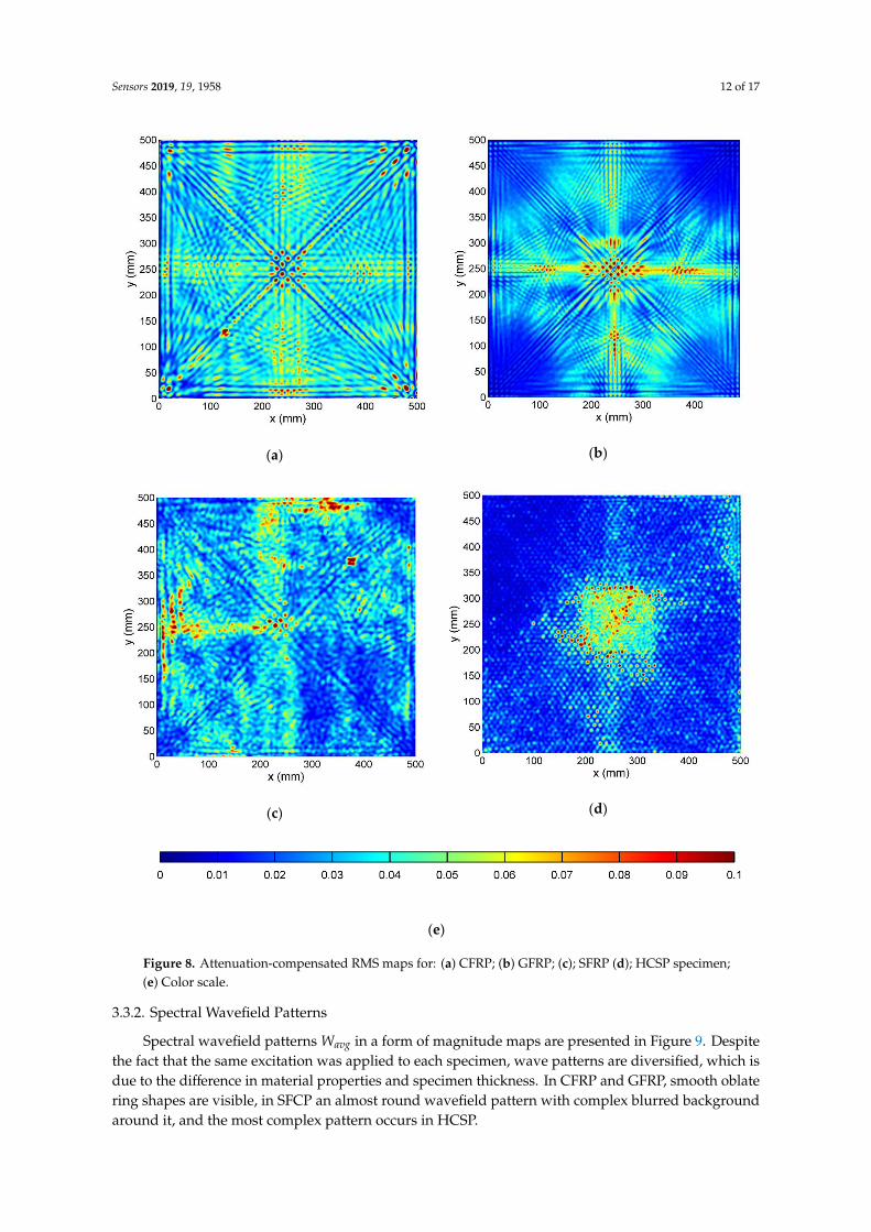
Figure 8. Attenuation-compensated RMS maps for: (a) CFRP; (b) GFRP; (c); SFRP (d); HCSP specimen;
(e) Color scale.
3.3.2. Spectral Wavefield Patterns
Spectral wavefield patterns Wavg in a form of magnitude maps are presented in Figure 9. Despite
the fact that the same excitation was applied to each specimen, wave patterns are diversified, which
is due to the difference in material properties and specimen thickness. In CFRP and GFRP, smooth
oblate ring shapes are visible, in SFCP an almost round wavefield pattern with complex blurred
background around it, and the most complex pattern occurs in HCSP.
Figure 8. Attenuation-compensated RMS maps for: (a) CFRP; (b) GFRP; (c); SFRP (d); HCSP specimen;(e) Color scale.
3.3.2. Spectral Wavefield Patterns
Spectral wavefield patterns Wavg in a form of magnitude maps are presented in Figure 9. Despitethe fact that the same excitation was applied to each specimen, wave patterns are diversified, which isdue to the difference in material properties and specimen thickness. In CFRP and GFRP, smooth oblatering shapes are visible, in SFCP an almost round wavefield pattern with complex blurred backgroundaround it, and the most complex pattern occurs in HCSP.

Sensors 2019, 19, 1958 13 of 17Sensors 2019, 19, x FOR PEER REVIEW 13 of 17
(a)
(b)
(c)
(d)
(e)
Figure 9. Wavefield patterns in wavenumber domain for: (a) CFRP; (b) GFRP; (c); SFRP (d); HCSP
specimen; (e) Color scale.
By thresholding of wavefield patterns, filter masks were determined, and are presented in Figure
10, where the black areas stand for 0 value, and they light grey areas stand for 1.
Figure 9. Wavefield patterns in wavenumber domain for: (a) CFRP; (b) GFRP; (c); SFRP (d); HCSPspecimen; (e) Color scale.
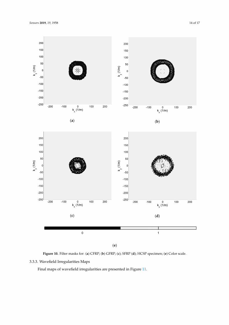
By thresholding of wavefield patterns, filter masks were determined, and are presented inFigure 10, where the black areas stand for 0 value, and they light grey areas stand for 1.
Sensors 2019, 19, 1958 14 of 17Sensors 2019, 19, x FOR PEER REVIEW 14 of 17
(a)
(b)
(c)
(d)
(e)
Figure 10. Filter masks for: (a) CFRP; (b) GFRP; (c); SFRP (d); HCSP specimen; (e) Color scale.
3.3.3. Wavefield Irregularities Maps
Final maps of wavefield irregularities are presented in Figure 11.
Teflon insert in the CFRP specimen (Figure 11a) is clearly visualized with its proper location,
size, and shape. Small amplitude values of the map in the center correspond to the PZT transducer.
In Figure 11b, all four delaminations are visible with the correct position and elongated by about
50%. Defect position in depth from the measured surface shows a correlation with obtained map
values. The closer the delamination is to the front surface of the specimen, the higher the value on the
presented map occurs.
Figure 10. Filter masks for: (a) CFRP; (b) GFRP; (c); SFRP (d); HCSP specimen; (e) Color scale.
3.3.3. Wavefield Irregularities Maps
Final maps of wavefield irregularities are presented in Figure 11.

Sensors 2019, 19, 1958 15 of 17
Sensors 2019, 19, x FOR PEER REVIEW 15 of 17
In the SFRP specimen (Figure 11c), due to a distorted wavefield by randomly distributed fibers,
small irregularities identification covers the whole specimen surface. However, the damage is clearly
visible with its shape and size, corresponding to the sample specification.
Crushed honeycomb filler edges in Figure 11d are well defined. Front plate deboning is visible
on the right side with additional high-value regions along the left and right edges. Only back panel
disbonding cannot be identified from these obtained maps. Its edge is barely visible and small
change in a dotted pattern inside this region may be noticed.
(a)
(b)
(c)
(d)
(e)
Figure 11. Wavefield irregularities map in: (a) CFRP; (b) GFRP; (c); SFRP (d); HCSP specimen; (e)
Color scale.
Figure 11. Wavefield irregularities map in: (a) CFRP; (b) GFRP; (c); SFRP (d); HCSP specimen; (e)Color scale.
Teflon insert in the CFRP specimen (Figure 11a) is clearly visualized with its proper location, size,and shape. Small amplitude values of the map in the center correspond to the PZT transducer.
In Figure 11b, all four delaminations are visible with the correct position and elongated by about50%. Defect position in depth from the measured surface shows a correlation with obtained map

Sensors 2019, 19, 1958 16 of 17
values. The closer the delamination is to the front surface of the specimen, the higher the value on thepresented map occurs.
In the SFRP specimen (Figure 11c), due to a distorted wavefield by randomly distributed fibers,small irregularities identification covers the whole specimen surface. However, the damage is clearlyvisible with its shape and size, corresponding to the sample specification.
Crushed honeycomb filler edges in Figure 11d are well defined. Front plate deboning is visibleon the right side with additional high-value regions along the left and right edges. Only back paneldisbonding cannot be identified from these obtained maps. Its edge is barely visible and small changein a dotted pattern inside this region may be noticed.
4. Discussion
In this work, a technique for mapping irregularities of propagating guided waves is proposed.It is used for damage detection, localization, and assessment. The effectiveness of this method wasverified experimentally on four various composite plates with defects. Guided waves were excited byPZT transducer, and measured by scanning laser vibrometer.
The main advantage of the proposed algorithm is its robustness, versatility and high efficacy. It isfully automatized, giving results easy to interpret. No a priori information about material properties orreference data is needed. It is suitable for the identification of a wide variety of manufacturing defectsand damage that would have occurred during structure operation in various composite materials.The algorithm uses fast Fourier transform implementation, and therefore is not computationallyintensive, while the processing of presented results took less than 5 s for each sample on a moderndesktop computer.
Further studies should be focused on testing the proposed method on a more complex,real structure.
Author Contributions: Conceptualization, P.K., M.R. and L.D.M.; methodology, P.K. and W.O.; software,L.D.M. and M.R.; validation, M.R. and A.M.; formal analysis, L.D.M.; investigation, M.R.; resources, W.O.;writing—original draft preparation, P.K. and M.R.; writing—review and editing, W.O. and A.M.; visualization,P.K.; supervision, W.O. and A.M.; project administration, W.O. and A.M.; funding acquisition, W.O.
Funding: The research was funded by the Polish National Science Centre under grant agreement noUMO-2012/06/M/ST8/00414 in the frame of HARMONIA project entitled: Investigation of elastic wave propagationphenomenon in composite materials with imperfections.
Conflicts of Interest: The authors declare no conflict of interest.
References
1. Wandowski, T.; Malinowski, P.H.; Ostachowicz, W.M. Circular sensing networks for guided waves basedstructural health monitoring. Mech. Syst. Signal Process. 2016, 66, 248–267. [CrossRef]
2. Malinowski, P.; Wandowski, T.; Ostachowicz, W. Damage detection potential of a triangular piezoelectricconfiguration. Mech. Syst. Signal Process. 2011, 25, 2722–2732. [CrossRef]
3. Wandowski, T.; Malinowski, P.; Ostachowicz, W.M. Damage detection with concentrated configurations ofpiezoelectric transducers. Smart Mater. Struct. 2011, 20, 025002. [CrossRef]
4. Wandowski, T.; Malinowski, P.; Ostachowicz, W. Diagnostics using different configurations of sensingnetworks. J. Phys. Conf. Ser. 2011, 305, 012007. [CrossRef]
5. Kudela, P.; Radzienski, M.; Ostachowicz, W.; Yang, Z. Structural Health Monitoring system based on aconcept of Lamb wave focusing by the piezoelectric array. Mech. Syst. Signal Process. 2018, 108, 21–32.[CrossRef]
6. Giurgiutiu, V. Piezoelectric Wafer Active Sensors for Structural Health Monitoring of Composite StructuresUsing Tuned Guided Waves. J. Eng. Mater. Technol. 2011, 133, 041012. [CrossRef]
7. Michaels, J.E.; Michaels, T.E. Guided wave signal processing and image fusion for in situ damage localizationin plates. Wave Motion 2007, 44, 482–492. [CrossRef]
8. Rao, J.; Ratassepp, M.; Lisevych, D.; Hamzah Caffoor, M.; Fan, Z. On-Line Corrosion Monitoring of PlateStructures Based on Guided Wave Tomography Using Piezoelectric Sensors. Sensors 2017, 17, 2882. [CrossRef]

Sensors 2019, 19, 1958 17 of 17
9. Bijudas, C.R.; Mitra, M.; Mujumdar, P.M. Time reversed Lamb wave for damage detection in a stiffenedaluminum plate. Smart Mater. Struct. 2013, 22, 105026. [CrossRef]
10. Wang, C.H.; Rose, J.T.; Chang, F.-K. A synthetic time-reversal imaging method for structural health monitoring.Smart Mater. Struct. 2004, 13, 415–423. [CrossRef]
11. Mitra, M.; Gopalakrishnan, S. Guided wave based structural health monitoring: A review. Smart Mater.Struct. 2016, 25, 053001. [CrossRef]
12. Wandowski, T.; Kudela, P.; Malinowski, P.; Ostachowicz, W. Lamb Waves for Damage Localisation in Panels.Strain 2011, 47, 449–457. [CrossRef]
13. Zhao, J.; Li, F.; Cao, X.; Li, H. Wave Propagation in Aluminum Honeycomb Plate and Debonding DetectionUsing Scanning Laser Vibrometer. Sensors 2018, 18, 1669. [CrossRef]
14. Ruzzene, M. Frequency–wavenumber domain filtering for improved damage visualization. Smart Mater.Struct. 2007, 16, 2116–2129. [CrossRef]
15. Park, B.; An, Y.-K.; Sohn, H. Visualization of hidden delamination and debonding in composites throughnoncontact laser ultrasonic scanning. Compos. Sci. Technol. 2014, 100, 10–18. [CrossRef]
16. Tian, Z.; Leckey, C.; Rogge, M.; Yu, L. Crack detection with Lamb wave wavenumber analysis. In Proceedingsof the International Society for Optics and Photonics, San Diego, CA, USA, 11–14 March 2013; p. 86952Z.
17. Ruzzene, M. Simulation and Measurement of Ultrasonic Waves in Elastic Plates Using Laser Vibrometry.AIP Conf. Proc. 2005, 760, 172–179. [CrossRef]
18. Radzienski, M.; Dolinski, Ł.; Krawczuk, M.; Zak, A.; Ostachowicz, W. Application of RMS for damagedetection by guided elastic waves. J. Phys. Conf. Ser. 2011, 305, 012085. [CrossRef]
19. Staszewski, W.J.; Lee, B.C.; Traynor, R. Fatigue crack detection in metallic structures with Lamb waves and3D laser vibrometry. Meas. Sci. Technol. 2007, 18, 727–739. [CrossRef]
20. Ostachowicz, W.; Radzienski, M.; Kudela, P. 50th Anniversary Article: Comparison Studies of Full WavefieldSignal Processing for Crack Detection. Strain 2014, 50, 275–291. [CrossRef]
21. An, Y.-K.; Park, B.; Sohn, H. Complete noncontact laser ultrasonic imaging for automated crack visualizationin a plate. Smart Mater. Struct. 2013, 22, 025022. [CrossRef]
22. Kudela, P.; Radzienski, M.; Ostachowicz, W. Identification of cracks in thin-walled structures by means ofwavenumber filtering. Mech. Syst. Signal Process. 2015, 50–51, 456–466. [CrossRef]
23. Kudela, P.; Radzienski, M.; Ostachowicz, W. Impact induced damage assessment by means of Lamb waveimage processing. Mech. Syst. Signal Process. 2018, 102, 23–36. [CrossRef]
© 2019 by the authors. Licensee MDPI, Basel, Switzerland. This article is an open accessarticle distributed under the terms and conditions of the Creative Commons Attribution(CC BY) license (http://creativecommons.org/licenses/by/4.0/).