Damage identification for high-speed railway truss arch bridge using fuzzy clustering analysis

Baoya Cao1a, Youliang Ding*2, Hanwei Zhao3 and Yongsheng Song4

1,2,3 The Key Laboratory of Concrete and Prestressed Concrete Structures of Ministry of

Education, Southeast University, Nanjing 210096, China 4 Jinling Institute of Technology, Nanjing 211169, China

Abstract

This study aims to do damage identification for Da-Sheng-Guan(DSG) high-speed railway truss arch bridge using fuzzy clustering analysis. Firstly, structural health monitoring(SHM) system is established for the DSG Bridge. Long-term field monitoring strain data in 8 different cases caused by high-speed trains are taken as classification reference for other unknown cases. And finite element model(FEM) of DSG Bridge is established to simulate damage cases of the bridge. Then, effectiveness of one fuzzy clustering analysis method named transitive closure method and FEM results are verified using the monitoring strain data. Three standardization methods at the first step of fuzzy clustering transitive closure method are compared: extreme difference method, maximum method and non-standard method, while non-standard method turns out to be the best. At last, the fuzzy clustering method is taken to identify damage in different degree and different locations. The results show that when the strain model change caused by damage is more than it caused by different carriages, the damage in DSG bridge is identified.

Keywords: railway bridge; steel truss arch; structural health monitoring; damage identification; fuzzy clustering; finite element analysis1 Introduction`

1. Introduction

In the past few decades, structural health monitoring (SHM) has been one of the most

popular research areas in the bridge engineering field (Garden and Fanning 2004,

Farrar and Worden 2007, Ou and Li 2010 and Yu and Xu 2011). SHM process is to

collect data from the monitored structure using periodically sampled measurements by

* Corresponding author, Professor, E-mail: civilchina@hotmail.com

a Ph.D. Student, E-mail: caobaoya@outlook.com

an array of sensors, then extract features from these measurements and conduct

statistical analysis of these features to assess the structural degradation (Fan and Qiao

2011, Sabatto et al. 2011 and Kovvali et al. 2007).

The detection of damage is the most fundamental issue in SHM. Damage may be

defined as a state of change that affects the present or future performance of a system.

Implicit in the above definition is the fact that damage detection involves comparison

with some initial undamaged state (Meyyappan et al. 2003). In this project the sensors

were connected to the bridge, which was monitored. SHM system with a great quantity

of various types of sensors is usually employed by large infrastructure engineering for

long-term health monitoring. Except field monitoring method, test and numerical

simulation methods are also adopted as a supplement in research (Yu et al. 2011 and

Erdogan et al. 2014). The numerical analysis model is calibrated using SHM data and

better represents the existing structure behavior under different loading conditions.

Recently, fuzzy approaches have been applied to solve problems related to damage

detection. Fuzzy logic is utilized to handle uncertainties and imprecision involved. Fuzzy

clustering is an unsupervised learning operation that aims at decomposing a given set of

objects into subgroups or clusters based on similarity. The goal is to divide the dataset in

such a way that objects or cases belonging to the same cluster are as similar as

possible, whereas objects belonging to different clusters are dissimilar (Kruse et al.

2007). Fuzzy cluster analysis methods mainly include: transitive closure method based

on fuzzy equivalence relation, the method based on similarity relation and fuzzy

relationship, the maximum tree method based on fuzzy graph theory and the convex

decomposition based on data sets and the dynamic rules (Zhou et al. 2015).

Fuzzy clustering method has been used in many areas by researchers. Tarighat and

Miyamoto (2009) introduced a new fuzzy method to deal with uncertainties from

inspection data, which was practically based on both subjective and objective results of

existing inspection methods and tools. Wang and Elhag (2007) proposed a fuzzy group

decision making (FGDM) approach for bridge risk assessment. Silva et al. (2008)

compared two fuzzy clustering algorithms: fuzzy c-means (FCM) and Gustafson–Kessel

(GK) algorithms by applying them to data from a benchmark frame structure in the Los

Alamos National Laboratory. Palomino et al. (2014) and Salah et al. (2013) use fuzzy

cluster analysis methods for aircraft's damage classification. Zhou et al. (2015) evaluate

health state of shield tunnel SHM using fuzzy cluster method. Zhao and Chen (2002)

use fuzzy inference system to do concrete bridge deterioration diagnosis. Jiao et al.

(2013) assess durability of the bridge based on fuzzy clustering and field data.

Meyyappaq et al. (2003) has done damage accumulation analysis based on bridge

health monitoring vibration data using fuzzy-neuro system.

Even though many researches have done damage analysis of different kinds of

structures using fuzzy logic, there are few studies on high-speed railway truss arch

bridges according to previous studies, especially based on field monitoring data.

Nanjing DSG Bridge is a steel truss arch bridge with the longest span throughout the

world. Its 336m main span and 6-track railways rank itself the largest bridge with

heaviest design loading among the high-speed railway bridges by far. And the design

speed 300km/h is also on the advanced level in the world. Thus damage identification of

DSG Bridge is valuable. In this study, long-term field monitoring sensors are installed on

the Nanjing DSG Bridge to collect strain extreme value caused by high-speed trains.

The finite element model of DSG Bridge is also established to research damage as a

supplement. Then, effectiveness of fuzzy clustering method and FEM results are verified

using SHM data. Three standard methods are compared in the fuzzy clustering method.

Finally, the fuzzy clustering method is taken to identify damage with different degree and

location.

2. SHM system and finite element model of the bridge

2.1 SHM system

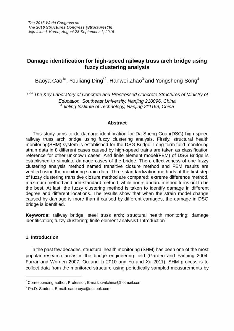
The panoramic view of Nanjing DSG Bridge is shown in Fig. 1(a), which is a steel

truss arch bridge with the span arrangement (108+192+336+336+192+108) m. The

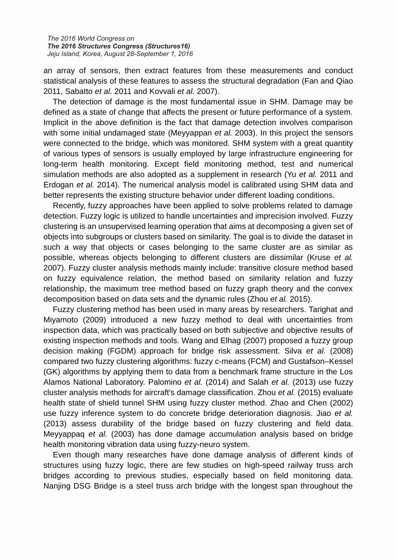
elevation drawing of the bridge is shown in Fig. 1(b). Due to the remarkable

characteristics of DSG Bridge including long span of the main girder, heavy design

loading and high speed of trains, a long-term SHM system was installed on the DSG

Bridge shortly after it was opened to railway traffic. As shown in Fig. 1(b), dynamic strain

monitoring of steel truss arch is performed at the 1-1, 2-2, 3-3 and 4-4 cross-section in

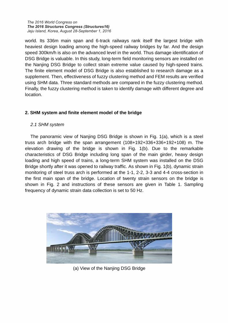
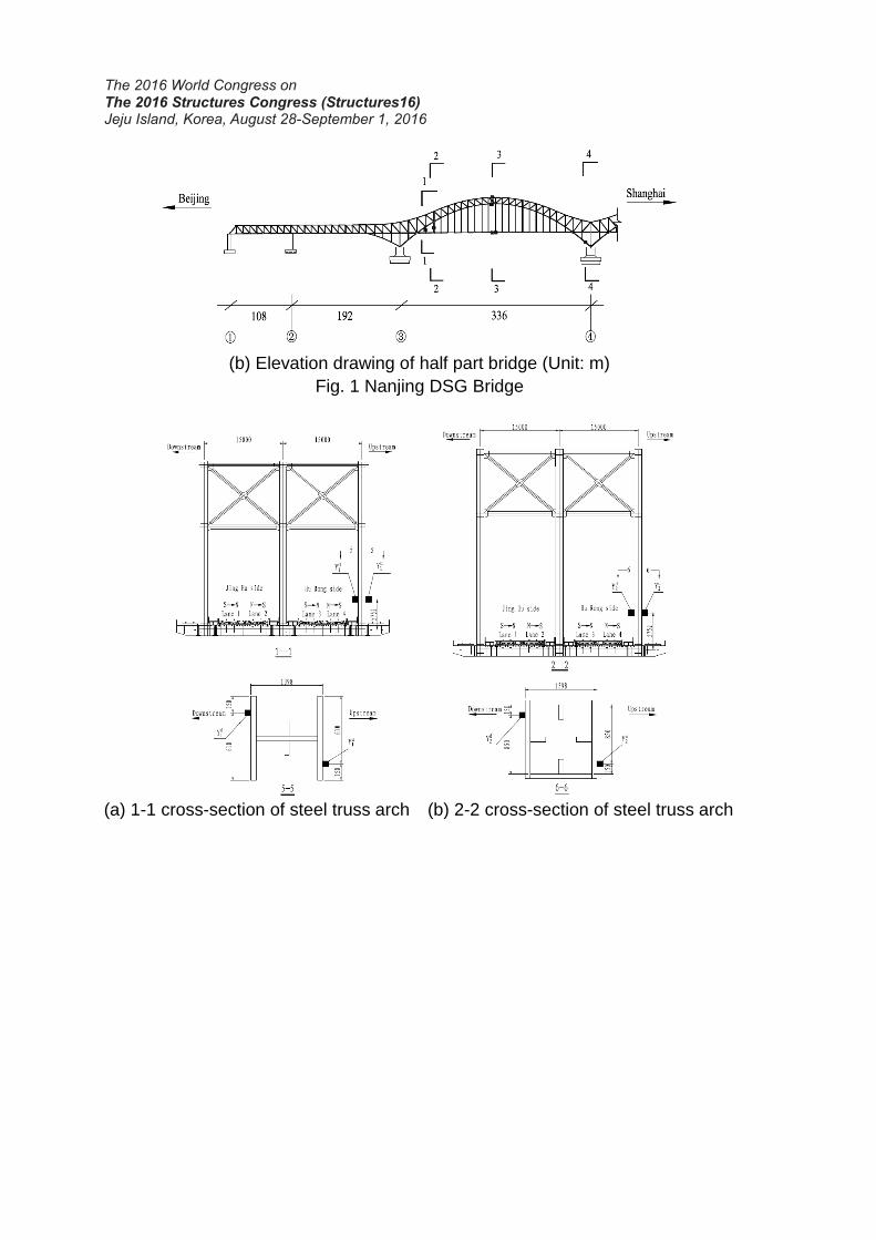
the first main span of the bridge. Location of twenty strain sensors on the bridge is

shown in Fig. 2 and instructions of these sensors are given in Table 1. Sampling

frequency of dynamic strain data collection is set to 50 Hz.

(a) View of the Nanjing DSG Bridge

(b) Elevation drawing of half part bridge (Unit: m)

Fig. 1 Nanjing DSG Bridge

(a) 1-1 cross-section of steel truss arch (b) 2-2 cross-section of steel truss arch

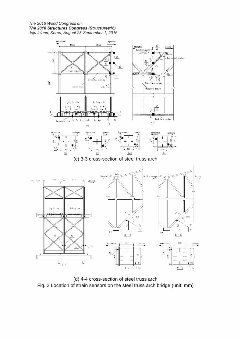
(c) 3-3 cross-section of steel truss arch

(d) 4-4 cross-section of steel truss arch

Fig. 2 Location of strain sensors on the steel truss arch bridge (unit: mm)

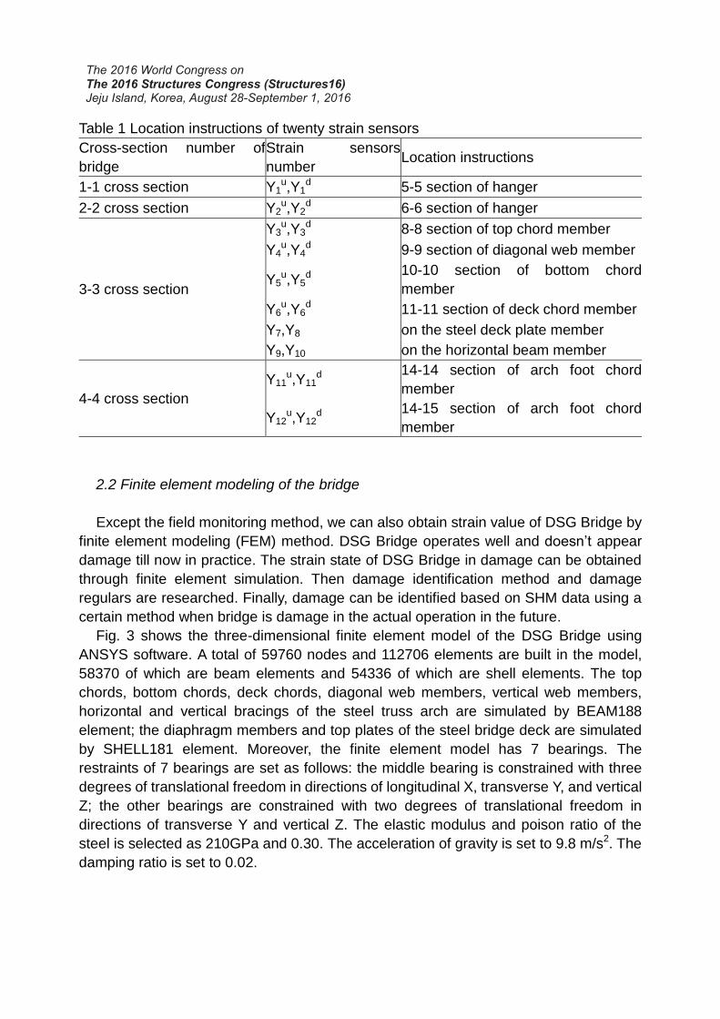
Table 1 Location instructions of twenty strain sensors

Cross-section number of

bridge

Strain sensors

number Location instructions

1-1 cross section Y1u,Y1

d 5-5 section of hanger

2-2 cross section Y2u,Y2

d 6-6 section of hanger

3-3 cross section

Y3u,Y3

d 8-8 section of top chord member

Y4u,Y4

d 9-9 section of diagonal web member

Y5u,Y5

d 10-10 section of bottom chord

member

Y6u,Y6

d 11-11 section of deck chord member

Y7,Y8 on the steel deck plate member

Y9,Y10 on the horizontal beam member

4-4 cross section

Y11u,Y11

d 14-14 section of arch foot chord

member

Y12u,Y12

d 14-15 section of arch foot chord

member

2.2 Finite element modeling of the bridge

Except the field monitoring method, we can also obtain strain value of DSG Bridge by

finite element modeling (FEM) method. DSG Bridge operates well and doesn’t appear

damage till now in practice. The strain state of DSG Bridge in damage can be obtained

through finite element simulation. Then damage identification method and damage

regulars are researched. Finally, damage can be identified based on SHM data using a

certain method when bridge is damage in the actual operation in the future.

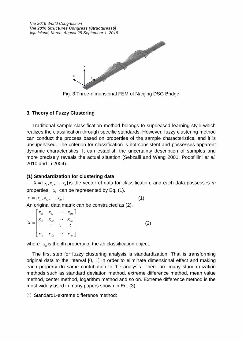
Fig. 3 shows the three-dimensional finite element model of the DSG Bridge using

ANSYS software. A total of 59760 nodes and 112706 elements are built in the model,

58370 of which are beam elements and 54336 of which are shell elements. The top

chords, bottom chords, deck chords, diagonal web members, vertical web members,

horizontal and vertical bracings of the steel truss arch are simulated by BEAM188

element; the diaphragm members and top plates of the steel bridge deck are simulated

by SHELL181 element. Moreover, the finite element model has 7 bearings. The

restraints of 7 bearings are set as follows: the middle bearing is constrained with three

degrees of translational freedom in directions of longitudinal X, transverse Y, and vertical

Z; the other bearings are constrained with two degrees of translational freedom in

directions of transverse Y and vertical Z. The elastic modulus and poison ratio of the

steel is selected as 210GPa and 0.30. The acceleration of gravity is set to 9.8 m/s2. The

damping ratio is set to 0.02.

X Y

Z

Fig. 3 Three-dimensional FEM of Nanjing DSG Bridge

3. Theory of Fuzzy Clustering

Traditional sample classification method belongs to supervised learning style which

realizes the classification through specific standards. However, fuzzy clustering method

can conduct the process based on properties of the sample characteristics, and it is

unsupervised. The criterion for classification is not consistent and possesses apparent

dynamic characteristics. It can establish the uncertainty description of samples and

more precisely reveals the actual situation (Sebzalli and Wang 2001, Podofillini et al.

2010 and Li 2004).

(1) Standardization for clustering data

1 2{ , , , }nX x x x is the vector of data for classification, and each data possesses m

properties. ix can be represented by Eq. (1).

1 2[ , , , ]i i i imx x x x (1)

An original data matrix can be constructed as (2).

11 12 1

21 22 2

1 2

m

m

n n nm

x x x

x x xX

x x x

(2)

where ijx is the jth property of the ith classification object.

The first step for fuzzy clustering analysis is standardization. That is transforming

original data to the interval [0, 1] in order to eliminate dimensional effect and making

each property do same contribution to the analysis. There are many standardization

methods such as standard deviation method, extreme difference method, mean value

method, center method, logarithm method and so on. Extreme difference method is the

most widely used in many papers shown in Eq. (3).

① Standard1-extreme difference method:

min'

max min

1,2, , ; 1,2, ,ij j

ij

j j

x xx i n j m

x x

(3)

max 1 2 min 1 2max , , , , min , , ,j j j nj j j j njx x x x x x x x

Step1: m i n 1, 2 , ; 1 , 2 ,i j i j jx x x i n j m

(4-a)

Step2:

'

max

1,2, , ; 1,2, ,ij

ij

j

xx i n j m

x (4-b)

Standard1 method can be divided into two steps just shown as Eqs. (4-a)- (4-b). The

first step shown in (4-a) is each member ijx in the original matrix subtracts the

minimum member minjx of each column. Then we get a new matrix. The second step

shown in (4-b) is each element ijx in the new matrix divided by the maximum

maxjx of

each column to transform data to the interval [0, 1]. As we can see the first step in this place is not necessary to eliminate dimensional effect. So we can try to skip the first step and only do the second step. This is standard2 method shown in Eq. (5).

② Standard2-the maximum method:

'

max

1,2, , ; 1,2, ,ij

ij

j

xx i n j m

x (5)

Take each row of the original data matrix for classification as a m dimension

vector1 2{ , , , }, 1,2,i i i imx x x x i n . Fuzzy clustering analysis is to compare the

relationship between these different rows according to the m different properties. Then do classification for the n row vectors. Both the two standard methods above has transformed the original data and brought changes in some extent about the relationship between the row vectors. And in the problem which will be analyzed in this paper, the dimensional for each property is the same. So we could also not standardizing the original data and don’t disturb the original characteristic at the most extent. This idea brings the third method that is non-standard method.

(2) Construction of fuzzy similarity matrix

Fuzzy similarity matrix is constructed mainly according to distance or ratio of data.

Similarity coefficient ijr is on behalf of similarity degree between ix and jx . ijr

calculation methods mainly includes dot product method, included angle cosine method, correlation coefficient method, exponent similarity coefficient, the maximum minimum

method and so on. In this paper, Similarity coefficient ijr will be get by calculating the

included angle cosine value between ix and jx . It is defined as (6):

' '

1

' 2 ' 2

1 1

, 1,2, ,

m

ik jk

kij

m m

ik jk

k k

x x

r i j n

x x

( ) (6)

(3) Calculate fuzzy equivalent matrix

The fuzzy similarity matrix calculated by (6) satisfies the reflexivity and symmetry but

doesn’t satisfy transitivity. The corresponding fuzzy equivalent matrix which satisfies

reflexivity, symmetry and transitivity must be obtained in order to do clustering analysis.

In this paper, successive square method is used to calculate the equivalent matrix as

shown in (7).

2( ) kR t R R , 2 2 1k kR R (7)

R is the fuzzy equivalent matrix. By selecting appropriate thresholds 0,1 ,

truncated matrix ( )R t R

is obtained.

(4) Determination of best classification

1 2, , , nX x x x is the object for classification. 1 2, , ,j j j jmx x x x

is the jth member

of ( 1,2, )X j n . And jkx is the kth feature of ( 1,2, , ).jx k m r is the classification

number corresponding to , and in is the number for the ith category. The average

value for kth eigenvalue of ith category can be calculated as shown in (8).

1

1, 1,2, ,

in

ik jk

ji

x x k mn

(8)

The average value for kth eigenvalue of all data can be calculated by Eq. (9).

1

1, 1, 2, ,

n

k jk

j

x x k mn

(9)

F-statistics analysis is used for determining the best classification threshold; it can be calculated by (10). F-statistics obeys distribution ( 1, )F r n r . Its numerator stands for

the distance between different categories while its denominator for the distance of samples in one category. So, the bigger F is, the further distance between different

categories is. If 0.05( 1, )F F r n r , the classification results is reasonable. And the bigger

(F-F0.05) value is, the better the classification results is.

2

1 1

2

1 1 1

( ) / ( 1)

( ) / ( )i

r m

i ik k

i k

nr m

jk ik

i j k

n x x r

F

x x n r

(10)

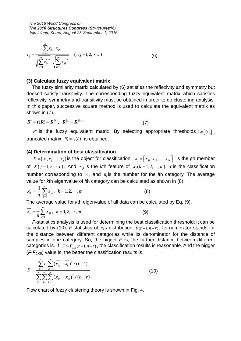
Flow chart of fuzzy clustering theory is shown in Fig. 4.

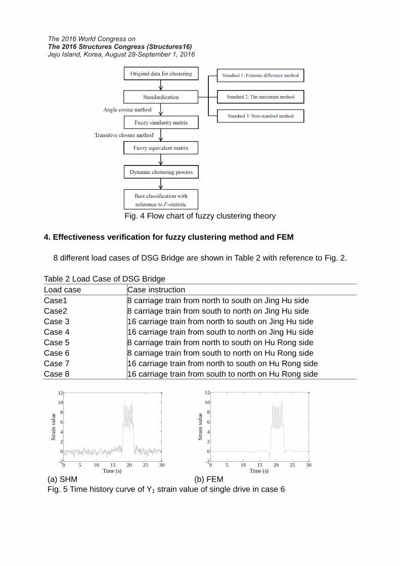
Fig. 4 Flow chart of fuzzy clustering theory

4. Effectiveness verification for fuzzy clustering method and FEM

8 different load cases of DSG Bridge are shown in Table 2 with reference to Fig. 2.

Table 2 Load Case of DSG Bridge

Load case Case instruction

Case1 8 carriage train from north to south on Jing Hu side

Case2 8 carriage train from south to north on Jing Hu side

Case 3 16 carriage train from north to south on Jing Hu side

Case 4 16 carriage train from south to north on Jing Hu side

Case 5 8 carriage train from north to south on Hu Rong side

Case 6 8 carriage train from south to north on Hu Rong side

Case 7 16 carriage train from north to south on Hu Rong side

Case 8 16 carriage train from south to north on Hu Rong side

0 5 10 15 20 25 30-2

0

2

4

6

8

10

12

Time (s)

Str

ain

valu

e

0 5 10 15 20 25 30

-2

0

2

4

6

8

10

12

Time (s)

Str

ain

valu

e

(a) SHM (b) FEM

Fig. 5 Time history curve of Y1 strain value of single drive in case 6

Strain value of deck plate members(Y7,Y8) and horizontal beam members(Y9,Y10) is

equal to stain sensor field monitoring value. But for truss members including hanger(Y1u,

Y1d, Y2

u, Y2d), web member(Y4

u, Y4d) and chord member(Y3

u, Y3d , Y5

u, Y5d , Y6

u, Y6d ,

Y11u, Y11

d , Y12u, Y12

d), the strain value is the mean of strain sensor monitoring value in

two sides of each truss member because truss members mainly subject axial stress. For

example, strain value Y1 is the mean value of Y1u and Y1

d. Y1 is the time history curve of

strain value when the train goes through the bridge, shown in Fig. 5. Strain extreme

MaxY1 and MinY1 is the maximum and minimum value of Y1, respectively.

Fig. 5(a) and (b) show Y1 strain value of signal drive in case 6 by field SHM method

and FEM simulation method, respectively. From Fig. 5 we can see: The results by SHM

and FEM are similar. The SHM data subject random disturbance outside, so the strain

value appear slight fluctuations. But the strain value acquired by the random

disturbance is much little than by trains. The slight fluctuations caused by random

disturbance can be ignored in this place. The curve pattern and strain value in Fig. 5(a)

and Fig. 5(b) is close. It indicates the FEM results are available.

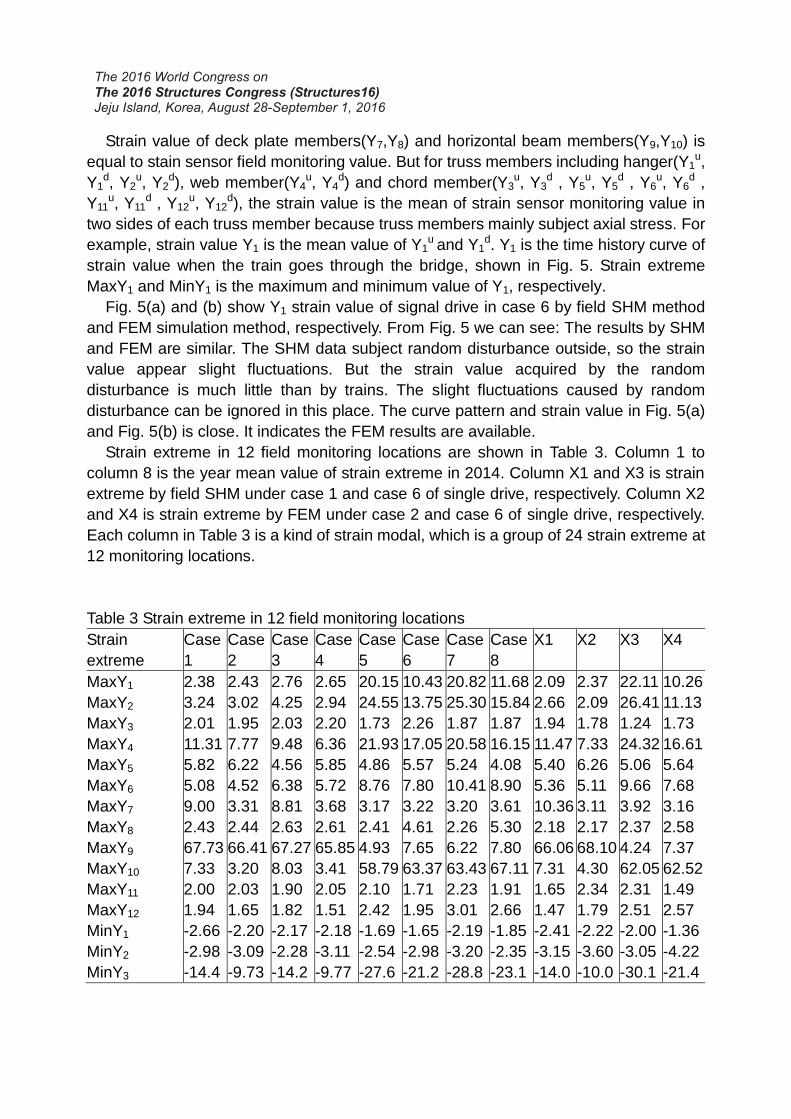
Strain extreme in 12 field monitoring locations are shown in Table 3. Column 1 to

column 8 is the year mean value of strain extreme in 2014. Column X1 and X3 is strain

extreme by field SHM under case 1 and case 6 of single drive, respectively. Column X2

and X4 is strain extreme by FEM under case 2 and case 6 of single drive, respectively.

Each column in Table 3 is a kind of strain modal, which is a group of 24 strain extreme at

12 monitoring locations.

Table 3 Strain extreme in 12 field monitoring locations

Strain

extreme

Case

1

Case

2

Case

3

Case

4

Case

5

Case

6

Case

7

Case

8

X1 X2 X3 X4

MaxY1 2.38 2.43 2.76 2.65 20.15 10.43 20.82 11.68 2.09 2.37 22.11 10.26

MaxY2 3.24 3.02 4.25 2.94 24.55 13.75 25.30 15.84 2.66 2.09 26.41 11.13

MaxY3 2.01 1.95 2.03 2.20 1.73 2.26 1.87 1.87 1.94 1.78 1.24 1.73

MaxY4 11.31 7.77 9.48 6.36 21.93 17.05 20.58 16.15 11.47 7.33 24.32 16.61

MaxY5 5.82 6.22 4.56 5.85 4.86 5.57 5.24 4.08 5.40 6.26 5.06 5.64

MaxY6 5.08 4.52 6.38 5.72 8.76 7.80 10.41 8.90 5.36 5.11 9.66 7.68

MaxY7 9.00 3.31 8.81 3.68 3.17 3.22 3.20 3.61 10.36 3.11 3.92 3.16

MaxY8 2.43 2.44 2.63 2.61 2.41 4.61 2.26 5.30 2.18 2.17 2.37 2.58

MaxY9 67.73 66.41 67.27 65.85 4.93 7.65 6.22 7.80 66.06 68.10 4.24 7.37

MaxY10 7.33 3.20 8.03 3.41 58.79 63.37 63.43 67.11 7.31 4.30 62.05 62.52

MaxY11 2.00 2.03 1.90 2.05 2.10 1.71 2.23 1.91 1.65 2.34 2.31 1.49

MaxY12 1.94 1.65 1.82 1.51 2.42 1.95 3.01 2.66 1.47 1.79 2.51 2.57

MinY1 -2.66 -2.20 -2.17 -2.18 -1.69 -1.65 -2.19 -1.85 -2.41 -2.22 -2.00 -1.36

MinY2 -2.98 -3.09 -2.28 -3.11 -2.54 -2.98 -3.20 -2.35 -3.15 -3.60 -3.05 -4.22

MinY3 -14.4 -9.73 -14.2 -9.77 -27.6 -21.2 -28.8 -23.1 -14.0 -10.0 -30.1 -21.4

2 4 4 8 8 7 9 3 5 6

MinY4 -12.3

2

-8.17 -9.07 -5.01 -22.4

2

-16.5

9

-19.7

4

-14.1

7

-11.4

7

-8.03 -24.2

2

-15.7

6

MinY5 -11.2

7

-8.61 -10.1

8

-7.47 -21.6

3

-16.8

1

-23.9

3

-18.2

8

-10.5

4

-8.93 -24.5

2

-16.8

6

MinY6 -2.98 -2.73 -2.32 -2.26 -3.61 -2.79 -3.38 -2.10 -2.94 -2.30 -3.55 -2.76

MinY7 -9.07 -3.04 -8.79 -3.50 -3.31 -3.31 -2.97 -3.24 -10.7

5

-2.62 -2.93 -2.79

MinY8 -2.37 -2.36 -2.71 -2.26 -3.34 -3.25 -4.04 -4.10 -2.21 -2.39 -3.35 -3.33

MinY9 -3.91 -3.23 -3.87 -3.88 -13.7

2

-7.06 -17.4

4

-6.85 -3.54 -3.98 -14.3

6

-7.33

MinY10 -6.34 -12.2

4

-6.25 -13.6

3

-4.81 -4.07 -6.43 -5.22 -5.46 -12.1

5

-4.36 -3.10

MinY11 -13.5

0

-12.7

6

-15.5

2

-14.5

9

-11.4

5

-11.9

4

-14.6

1

-13.9

8

-13.0

6

-12.3

4

-12.3

7

-11.1

6

MinY12 -15.5

6

-19.5

8

-19.1

1

-24.6

9

-2.91 -5.78 -2.12 -6.06 -15.0

2

-19.5

8

-3.04 -5.23

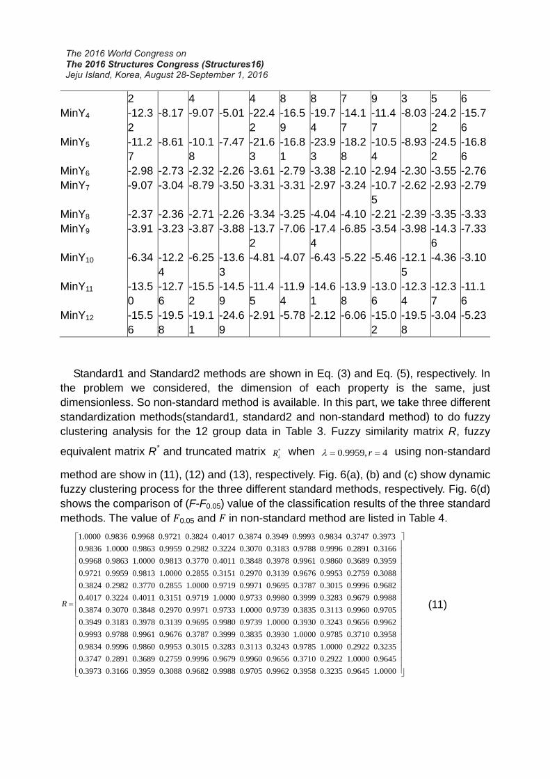
Standard1 and Standard2 methods are shown in Eq. (3) and Eq. (5), respectively. In

the problem we considered, the dimension of each property is the same, just

dimensionless. So non-standard method is available. In this part, we take three different

standardization methods(standard1, standard2 and non-standard method) to do fuzzy

clustering analysis for the 12 group data in Table 3. Fuzzy similarity matrix R, fuzzy

equivalent matrix R* and truncated matrix *R when 0.9959, 4r using non-standard

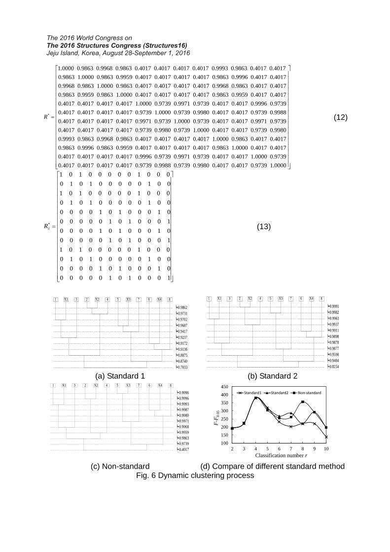
method are show in (11), (12) and (13), respectively. Fig. 6(a), (b) and (c) show dynamic

fuzzy clustering process for the three different standard methods, respectively. Fig. 6(d)

shows the comparison of (F-F0.05) value of the classification results of the three standard

methods. The value of 𝐹0.05 and 𝐹 in non-standard method are listed in Table 4.

1.0000 0.9836 0.9968 0.9721 0.3824 0.4017 0.3874 0.3949 0.9993 0.9834 0.3747 0.3973

0.9836 1.0000 0.9863 0.9959 0.2982 0.3224 0.3070 0.3183 0.9788 0.9996 0.2891 0.3166

0.9968

R

0.9863 1.0000 0.9813 0.3770 0.4011 0.3848 0.3978 0.9961 0.9860 0.3689 0.3959

0.9721 0.9959 0.9813 1.0000 0.2855 0.3151 0.2970 0.3139 0.9676 0.9953 0.2759 0.3088

0.3824 0.2982 0.3770 0.2855 1.0000 0.9719 0.9971 0.9695 0.3787 0.3015 0.9996 0.9682

0.4017 0.3224 0.4011 0.3151 0.9719 1.0000 0.9733 0.9980 0.3999 0.3283 0.9679 0.9988

0.3874 0.3070 0.3848 0.2970 0.9971 0.9733 1.0000 0.9739 0.3835 0.3113 0.9960 0.9705

0.3949 0.3183 0.3978 0.3139 0.9695 0.9980 0.9739 1.0000 0.3930 0.3243 0.9656 0.9962

0.9993 0.9788 0.9961 0.9676 0.3787 0.3999 0.3835 0.3930 1.0000 0.9785 0.3710 0.3958

0.9834 0.9996 0.9860 0.9953 0.3015 0.3283 0.3113 0.3243 0.9785 1.0000 0.2922 0.3235

0.3747 0.2891 0.3689 0.2759 0.9996 0.9679 0.9960 0.9656 0.3710 0.2922 1.0000 0.9645

0.3973 0.3166 0.3959 0.3088 0.9682 0.9988 0.9705 0.9962 0.3958 0.3235 0.9645 1.0000

(11)

*

1.0000 0.9863 0.9968 0.9863 0.4017 0.4017 0.4017 0.4017 0.9993 0.9863 0.4017 0.4017

0.9863 1.0000 0.9863 0.9959 0.4017 0.4017 0.4017 0.4017 0.9863 0.9996 0.4017 0.4017

0.9968

R

0.9863 1.0000 0.9863 0.4017 0.4017 0.4017 0.4017 0.9968 0.9863 0.4017 0.4017

0.9863 0.9959 0.9863 1.0000 0.4017 0.4017 0.4017 0.4017 0.9863 0.9959 0.4017 0.4017

0.4017 0.4017 0.4017 0.4017 1.0000 0.9739 0.9971 0.9739 0.4017 0.4017 0.9996 0.9739

0.4017 0.4017 0.4017 0.4017 0.9739 1.0000 0.9739 0.9980 0.4017 0.4017 0.9739 0.9988

0.4017 0.4017 0.4017 0.4017 0.9971 0.9739 1.0000 0.9739 0.4017 0.4017 0.9971 0.9739

0.4017 0.4017 0.4017 0.4017 0.9739 0.9980 0.9739 1.0000 0.4017 0.4017 0.9739 0.9980

0.9993 0.9863 0.9968 0.9863 0.4017 0.4017 0.4017 0.4017 1.0000 0.9863 0.4017 0.4017

0.9863 0.9996 0.9863 0.9959 0.4017 0.4017 0.4017 0.4017 0.9863 1.0000 0.4017 0.4017

0.4017 0.4017 0.4017 0.4017 0.9996 0.9739 0.9971 0.9739 0.4017 0.4017 1.0000 0.9739

0.4017 0.4017 0.4017 0.4017 0.9739 0.9988 0.9739 0.9980 0.4017 0.4017 0.9739 1.0000

(12)

*

1 0 1 0 0 0 0 0 1 0 0 0

0 1 0 1 0 0 0 0 0 1 0 0

1 0 1 0 0 0 0 0 1 0 0 0

0 1 0 1 0 0

R

0 0 0 1 0 0

0 0 0 0 1 0 1 0 0 0 1 0

0 0 0 0 0 1 0 1 0 0 0 1

0 0 0 0 1 0 1 0 0 0 1 0

0 0 0 0 0 1 0 1 0 0 0 1

1 0 1 0 0 0 0 0 1 0 0 0

0 1 0 1 0 0 0 0 0 1 0 0

0 0 0 0 1 0 1 0 0 0 1 0

0 0 0 0 0 1 0 1 0 0 0 1

(13)

1 X1 3 2 X2 4 5 X3 7 6 X4 8

┡=0.9862

┡=0.9731

┡=0.9702

┡=0.9687

┡=0.9417

┡=0.9237

┡=0.9172

┡=0.9136

┡=0.8875

┡=0.8740

┡=0.7033

1 X1 3 2 X2 4 5 X3 7 6 X4 8

┡=0.9991

┡=0.9982

┡=0.9963

┡=0.9937

┡=0.9911

┡=0.9898

┡=0.9878

┡=0.9877

┡=0.9598

┡=0.9484

┡=0.8234 (a) Standard 1 (b) Standard 2

1 X1 3 2 X2 4 5 X3 7 6 X4 8

┡=0.9996

┡=0.9996

┡=0.9993

┡=0.9987

┡=0.9980

┡=0.9971

┡=0.9968

┡=0.9959

┡=0.9863

┡=0.9739

┡=0.4017

100

150

200

250

300

350

400

450

2 3 4 5 6 7 8 9 10

F-F

0.0

5

Classification number r

Standard1 Standard2 Non-standard

(c) Non-standard (d) Compare of different standard method Fig. 6 Dynamic clustering process

Table 4 The value of 𝐹0.05 and 𝐹 in non-standard method

r 2 3 4 5 6 7 8 9 10 11

F 196.44 227.87 384.07 309.27 260.37 267.83 361.47 301.70 217.21 113.46

F0.05

4.96 4.60 4.07 4.12 4.39 4.95 6.09 8.85 19.40 242

F-F0.05 191.48 223.27 380.00 305.15 255.98 262.88 355.38 292.85 197.81 -128.54

From Fig. 6 and Table 4 we can see:

(1) The same characteristics of the three standard methods

① X1 gets into case 1 before others, and X3 gets into case 5 before others. Therefore,

X1 belongs to case 1 and X3 belongs to case 5. Clustering results are consistent with

field SHM results. So, this clustering method is credible.

② X2 gets into case 2 before others, and X4 gets into case 6 before others. Therefore,

X2 belongs to case 2 and X4 belongs to case 6. Clustering results are consistent with

FEM results. So, FEM results are credible.

③As it is mentioned above that the bigger (F-F0.05) value is, the better the clustering

result is. For these three methods, (F-F0.05) gets the maximum value 380 when

classification member r equals to 4. The corresponding truncated matrix R

is shown in

(3). At this time the clustering result is: {case 1, X1, case3}, {case 2, X2, case4}, {case 5,

X3, case7}, {case 6, X4, case8}. It means that the clustering result is the best when 8

carriage and 16 carriage train in the same line are in a category.

④At last, {case 1, X1, case3, case 2, X2, case4} and {case 5, X3, case7, case 6, X4,

case8} become a big category, respectively. It means Jing Hu side and Hu Rong side

become a category, respectively. At this time, classification member r equals to 2,

(F-F0.05) value is 191.48. This category result is not good.

(2) The different characteristics of the three standard methods

① The bigger (F-F0.05) value is, the better the clustering result is. It means that the

higher the curve in the Fig. 4(d) is, the better the standard method is. So from Fig. 4(d)

we can get the conclusion that: standard2 method is better than standard1 and

non-standard method is the best.

② In the Fig. 4(d), for non-standard method the curve gets another extreme value

355.38 when classification member r equals to 8. This extreme value is just a little less

than the maximum value 380 and more than others. It indicates that the clustering result

is also good when classification member r equals to 8. At this time the clustering result

is: {case 1, X1}, {case3}, {case 2, X2}, {case4}, {case 5, X3}, {case7}, {case 6, X4},

{case8}. This clustering result means each case in Table 1 is in a category. The result is

reasonable according to practical situation. However, standard1 and standard2 methods

can’t recognize this extreme point when r equals to 8. It also indicates that non-standard

method is better than the other two methods in this problem.

(3) The reason for the difference of the three standard methods

What brings the different results of the three standard methods? As we have

mentioned in section 3, we need to maintain the characteristic of original data and not to

disturb the relationship between the original row vectors at the most extent. The less the

original data is disturbed, the more the result is close to real situation. From standard1 to

sandand2 to non-standard method, the results becomes more and more reasonable

because of the transform operation becomes less and less. So we will use non-standard

method to do fuzzy clustering analysis below.

5. Damage Identification using fuzzy clustering analysis

Bridge may appear different degree damage after used for a period of time. Damage

identification is a fundamental issue in bridge health monitoring. FEM method is taken to

simulate bridge damage as the FEM results are credible illustrated in section 4. Then we

try to identify damage by non-standard fuzzy clustering analysis method.

5.1 Damage in different degree

As a typical representative, all the damage simulation by FEM given below is in the

case 6. Table 5 gives strain extreme value of the 12 monitoring locations at different

degree damage of bottom chord member Y5 which is at side truss of the mid-span. The

variable name Dam0, Dam10~ Dam50 in Table 4 means the area of chord member

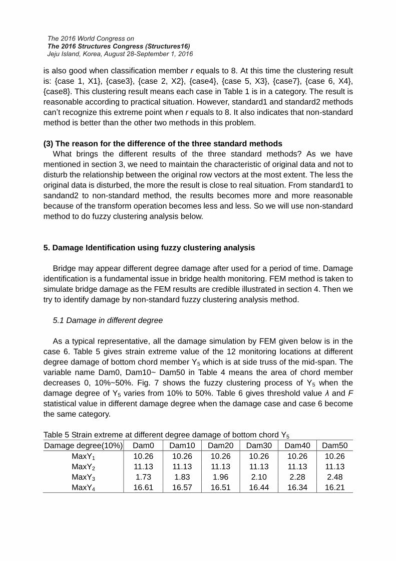
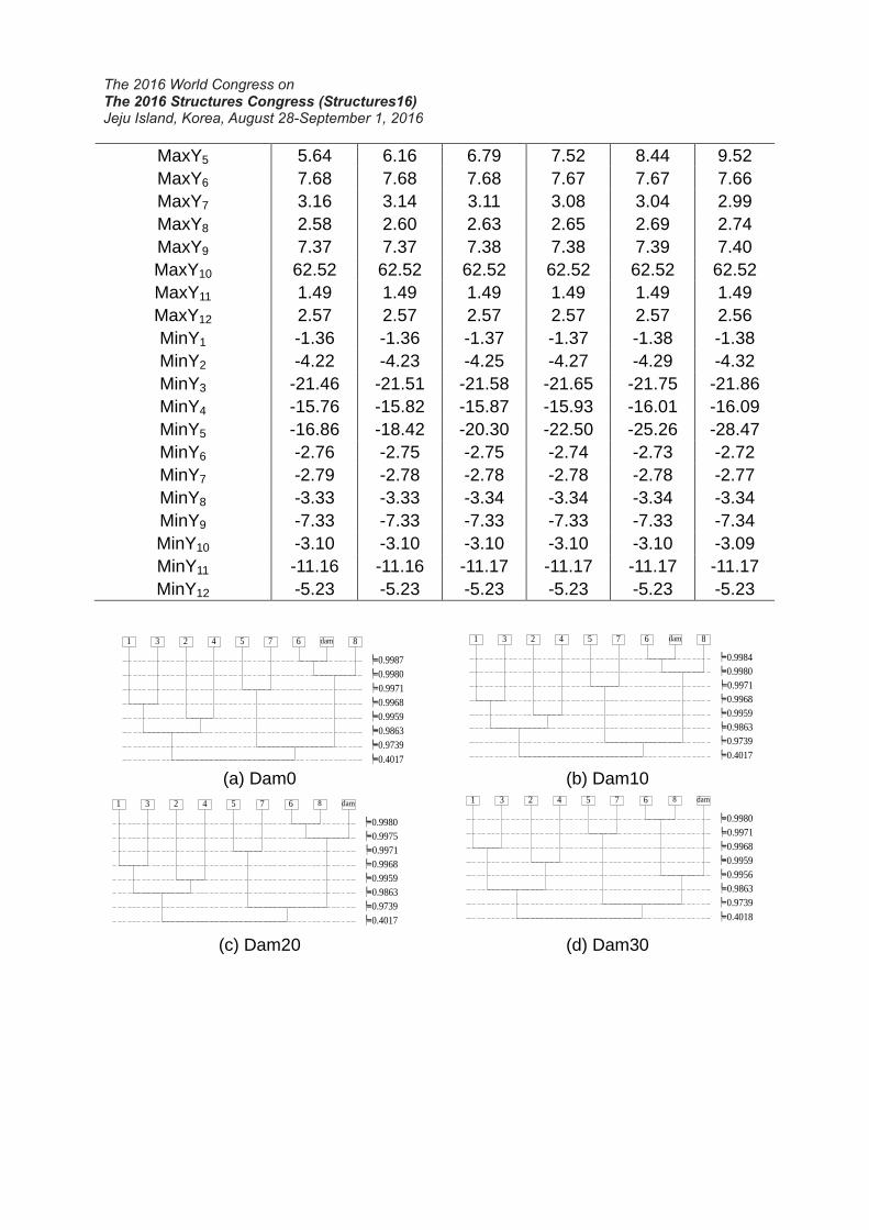
decreases 0, 10%~50%. Fig. 7 shows the fuzzy clustering process of Y5 when the

damage degree of Y5 varies from 10% to 50%. Table 6 gives threshold value λ and F

statistical value in different damage degree when the damage case and case 6 become

the same category.

Table 5 Strain extreme at different degree damage of bottom chord Y5

Damage degree(10%) Dam0 Dam10 Dam20 Dam30 Dam40 Dam50

MaxY1 10.26 10.26 10.26 10.26 10.26 10.26

MaxY2 11.13 11.13 11.13 11.13 11.13 11.13

MaxY3 1.73 1.83 1.96 2.10 2.28 2.48

MaxY4 16.61 16.57 16.51 16.44 16.34 16.21

MaxY5 5.64 6.16 6.79 7.52 8.44 9.52

MaxY6 7.68 7.68 7.68 7.67 7.67 7.66

MaxY7 3.16 3.14 3.11 3.08 3.04 2.99

MaxY8 2.58 2.60 2.63 2.65 2.69 2.74

MaxY9 7.37 7.37 7.38 7.38 7.39 7.40

MaxY10 62.52 62.52 62.52 62.52 62.52 62.52

MaxY11 1.49 1.49 1.49 1.49 1.49 1.49

MaxY12 2.57 2.57 2.57 2.57 2.57 2.56

MinY1 -1.36 -1.36 -1.37 -1.37 -1.38 -1.38

MinY2 -4.22 -4.23 -4.25 -4.27 -4.29 -4.32

MinY3 -21.46 -21.51 -21.58 -21.65 -21.75 -21.86

MinY4 -15.76 -15.82 -15.87 -15.93 -16.01 -16.09

MinY5 -16.86 -18.42 -20.30 -22.50 -25.26 -28.47

MinY6 -2.76 -2.75 -2.75 -2.74 -2.73 -2.72

MinY7 -2.79 -2.78 -2.78 -2.78 -2.78 -2.77

MinY8 -3.33 -3.33 -3.34 -3.34 -3.34 -3.34

MinY9 -7.33 -7.33 -7.33 -7.33 -7.33 -7.34

MinY10 -3.10 -3.10 -3.10 -3.10 -3.10 -3.09

MinY11 -11.16 -11.16 -11.17 -11.17 -11.17 -11.17

MinY12 -5.23 -5.23 -5.23 -5.23 -5.23 -5.23

dam=0%

┡=0.9987

1 3 2 4 5 7 6 dam 8

┡=0.9980

┡=0.9971

┡=0.9968

┡=0.9959

┡=0.9863

┡=0.9739

┡=0.4017

┡=0.9984

1 3 2 4 5 7 6 dam 8

┡=0.9980

┡=0.9971

┡=0.9968

┡=0.9959

┡=0.9863

┡=0.9739

┡=0.4017

dam=10%

(a) Dam0 (b) Dam10

dam=20%

┡=0.9980

1 3 2 4 5 7 6 8 dam

┡=0.9975

┡=0.9971

┡=0.9968

┡=0.9959

┡=0.9863

┡=0.9739

┡=0.4017 dam=30%

┡=0.9980

1 3 2 4 5 7 6 8 dam

┡=0.9971

┡=0.9968

┡=0.9959

┡=0.9956

┡=0.9863

┡=0.9739

┡=0.4018

(c) Dam20 (d) Dam30

dam=40%

┡=0.9980

1 3 2 4 5 7 6 8 dam

┡=0.9971

┡=0.9968

┡=0.9959

┡=0.9922

┡=0.9863

┡=0.9739

┡=0.4032

dam=50%

┡=0.9980

1 3 2 4 5 7 6 8 dam

┡=0.9971

┡=0.9968

┡=0.9959

┡=0.9869

┡=0.9863

┡=0.9739

┡=0.4041

(e) Dam40 (f) Dam50 Fig. 7 Dynamic clustering process of Y5 when damage degree varied from 10% to 50%

Table 6 threshold value λ and F statistical value in different damage degree

Dam(%) 0 10 20 30 40 50

λ 0.9987 0.9984 0.9975 0.9956 0.9922 0.9869

F 306.54 264.63 174.01 100.64 55.56 31.91

F0.05 237 237 237 237 237 237

F-F0.05 69.54 27.63 -62.99 -136.36 -181.44 -205.09

As we have illustrated in section 4, an undamaged case must get into one of the 8

cases in Table 1 before the other 7 cases using this fuzzy clustering analysis method. If

an unknown case can’t getting into one of the 8 cases firstly. It means that this unknown

case does not belong to the 8 cases. That is to say, this unknown case is abnormal and

the bridge stress modal changes. Bridge may be damage. In this paper, simulation by

FEM is in the case 6. The threshold value λ is 0.9980 for case 6 and case 8 getting into

the same category. So if threshold value λ of an unknown case with case 6 is less than

0.9980. It means that the change of bridge stress modal caused by the unknown case is

more than caused by the different carriages in the same lane. So this unknown case is

abnormal and bridge may be damage. At this time, the unknown case is identified as

damage. Or just in brief, the damage case is identified.

From Fig. 7 and Table 6 we can see:

(1) When damage degree is no more than 10%, damage case gets into case 6 before

the other 7 cases. Threshold value λ is greater than 0.9980. The damage case can’t be

identified in the degree of 10%.

(2) When damage degree reaches to 20%, damage case gets into case 6 after case

8. Threshold value λ is less than 0.9980. It means that stress modal change caused by

damage in this degree is more than it caused by different carriages. So the damage

case can be identified when the damage degree is more than 20%.

(3) When damage degree reaches to 50%, damage case is getting into case 6 just

after case 8 and before others. It illustrates that stress modal change caused by

damage is no more than it caused by different lanes although the damage degree

reaches 50%.

(4) The higher the damage degree is, the lower threshold value λ and (F-F0.05) value

is. It means that the difference between damage case and case 6 increases with the

growth of damage degree.

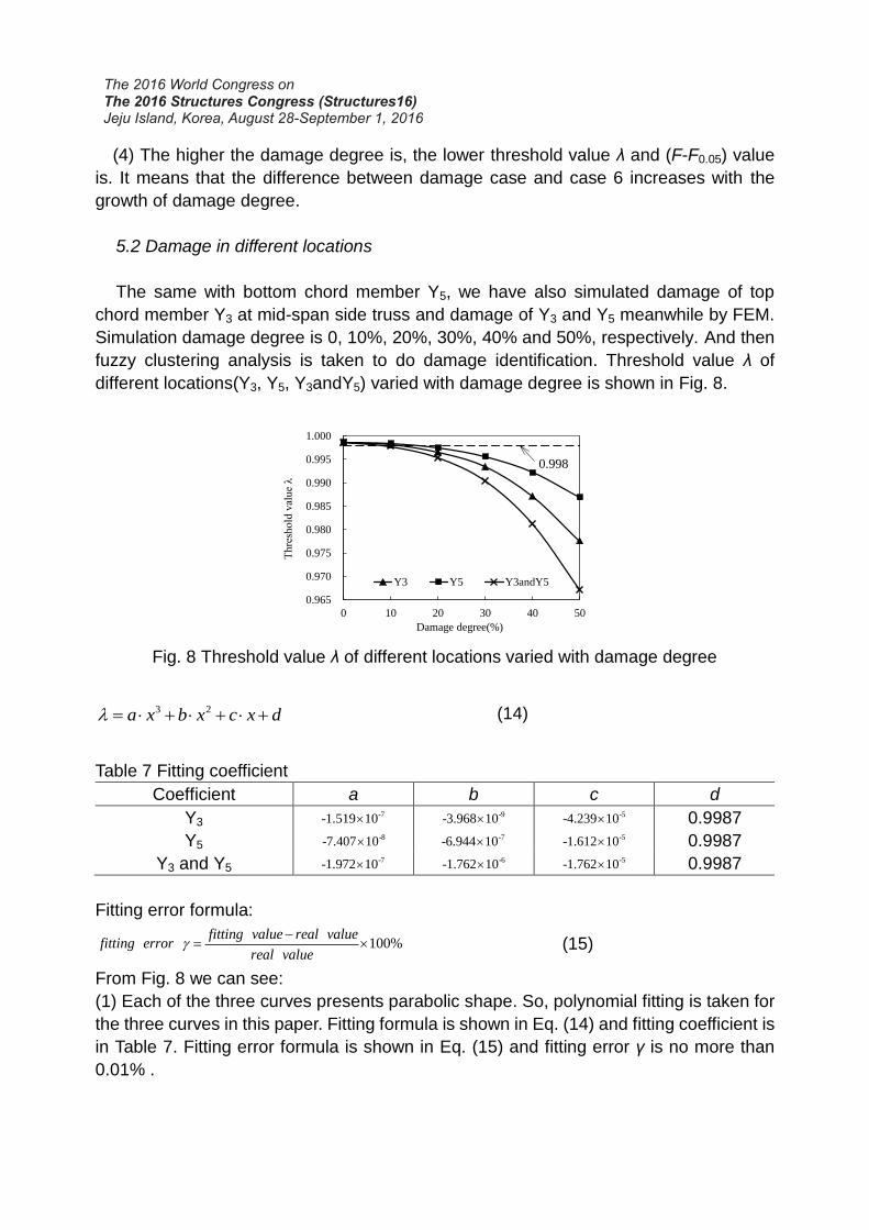
5.2 Damage in different locations

The same with bottom chord member Y5, we have also simulated damage of top

chord member Y3 at mid-span side truss and damage of Y3 and Y5 meanwhile by FEM.

Simulation damage degree is 0, 10%, 20%, 30%, 40% and 50%, respectively. And then

fuzzy clustering analysis is taken to do damage identification. Threshold value λ of

different locations(Y3, Y5, Y3andY5) varied with damage degree is shown in Fig. 8.

0.965

0.970

0.975

0.980

0.985

0.990

0.995

1.000

0 10 20 30 40 50

Thre

shold

val

ue

λ

Damage degree(%)

Y3 Y5 Y3andY5

0.998

Fig. 8 Threshold value λ of different locations varied with damage degree

3 2a x b x c x d (14)

Table 7 Fitting coefficient

Coefficient a b c d

Y3 -7-1.519 10 -9-3.968 10 -5-4.239 10 0.9987

Y5 -8-7.407 10 -7-6.944 10 -5-1.612 10 0.9987

Y3 and Y5 -7-1.972 10 -6-1.762 10 -5-1.762 10 0.9987

Fitting error formula:

100%fitting value real value

fitting errorreal value

(15)

From Fig. 8 we can see:

(1) Each of the three curves presents parabolic shape. So, polynomial fitting is taken for

the three curves in this paper. Fitting formula is shown in Eq. (14) and fitting coefficient is

in Table 7. Fitting error formula is shown in Eq. (15) and fitting error γ is no more than

0.01% .

(2) As it is referred in section 5.1, when threshold value λ of an unknown case getting

into case 6 is less than 0.998, this unknown case is identified as damage. Intersecting

x-coordinate of the curve Y3, Y5 and (Y3 and Y5) with λ=0.998 is 11.34, 15.64 and 8.80,

respectively. It indicates that for damage of Y3, damage of Y5, and damage of Y3 and Y5

at the same time, when the damage degree reaches to 11.34%, 15.64% and 8.8%,

respectively, the damage case can be identified. That is to say: bridge integrity is good,

local small degree damage(less than 10%) of one chord member will not bring obvious

changes of stress distribution modal. But when damage of one member reaches certain

degree or small damage occurs in two or more places, stress distribution modal will

produce obvious change and we should pay attention now.

(3) For the same degree, threshold value λ is different at different location. Top chord

member is more sensitive to damage than bottom chord member.

(4) The threshold value λ of Hu Rong side in the same category is 0.9739. When Y3 and

Y5 damage at the same time, λ is 0.9672 at the damage of 50%, less than 0.9739. That

is to say: when two locations damage at the same time and its damage degree reaches

50%, stress modal change caused by damage is more than caused by different lanes.

Damage is serious now.

6. Conclusion

In fuzzy clustering analysis, for the problem which dimension of different properties

is the same, the first step of standardization can be omitted as standardization is not

necessary at this time. The results may be better because any standardization method

disturbs the characteristic of original data while non-standard method keeps the

characteristic at the most extent.

We can identify an unknown case in field monitoring belongs to which one of the 8

cases by fuzzy clustering analysis method. If an unknown case gets into one of the 8

cases in Table 1 before the other 7 cases by fuzzy clustering analysis. This unknown

case belongs to this one.

We can identify bridge damage based on field monitoring data using fuzzy

clustering analysis method. If an unknown case can’t get into one of the 8 cases in Table

1 before the other 7 cases by fuzzy clustering analysis. The stress distribution model of

bridge changes obviously and the bridge may damage.

When either top chord or bottom chord member at side truss of the mid-span

damages, for the degree reaches 20%, its strain model change is obvious and the

damage can be identified. That is to say, when the damage exists in just one location, its

damage can be identified in a certain degree. This certain degree is varied with damage

location. It needs further research.

When top and bottom chord member at side truss of the mid-span damage at the

same time, for the damage degree is 10%, its strain model change is obvious and can

be identified. For the damage degree reaches 50%, its strain model change caused by

damage is more than caused by different lanes. That is to say, when bridge is damage

at two locations or more at the same time, its stain model changes obviously and its

damage can be identified at small degree. When damage reaches a certain degree, its

stain model changes a lot, damage is serious.

The curve of threshold value λ which is damage case and its corresponding case

being the same category varied with damage degree presents parabolic shape and can

be fitted with a cubic polynomial well.

Acknowledgement

The authors gratefully acknowledge the National Basic Research Program of China

(973 Program) (2015CB060000), the National Science and Technology Support

Program of China (2014BAG07B01), the National Natural Science Foundation

(51578138 & 51508070), the Program of “Six Major Talent Summit” Foundation

(1105000268), the Fundamental Research Funds for the Central Universities and

Priority Academic Program Development of Jiangsu Higher Education Institutions (No. ).

References

Garden, P.E. and Fanning, P.A. (2004), “Vibration based condition monitoring: a review”,

Structural Health Monitoring, 3(4), 355-377.

Farrar, C.R. and Worden, K. (2007), “An introduction to structural health monitoring.

Philosophical Transactions of the Royal Society”, 365, 303-315.

Ou, J.P. and Li, H. (2010), “Structural health monitoring in mainland China: review and

future trends. Structural Health Monitoring”, 9(3), 219-231.

Yu, L. and Xu., P. (2011), “Structural health monitoring based on continuous ACO

method. Microelectronics Reliability”, 51(2), 270-278.

Fan, W. and Qiao., P.Z. (2011), “Vibration-based damage identification methods: a

review and comparative study. Structural Health Monitoring”, 10(1), 83-111.

Sabatto, S. Zein, Mikhail, M., Bodruzzaman, M. and DeSimio, M. (2011), “Information

and Decision Fusion Systems for Aircraft Structural Health Monitoring, Southeastcon”,

IEEE Southeast Con 2011-Building Global Engineers, Nashville, TN, 395-400.

Kovvali, N., Das, S., Chakraborty, D., Cochran, D., Suppappola, A.P. and

Chattopadhyay, A.(2007), “Time Frequency Based Classification of Structural

Damage”, 48th IAA/ASME/ASCE/AHS/ACS, Structure Dynamic and Material

Conference, Honolulu, Hawaii.

Meyyappan, L., Jose, M., Dagli, C., Silva, P. and Pottinger, H. (2003), “Fuzzy-neuro

System for Bridge Health Monitoring”, 22nd International Conference of the North

American Fuzzy Information Processing Society, Chicago, IL, 8-13.

Yu, L., Zhu, J.H. and Yu, L.L. (2011), “Structural Damage Detection in a Truss Bridge

Model Using Fuzzy Clustering and Measured FRF Data Reduced by Principal

Component Projection”, 14th Asia Pacific Vibration Conference on Dynamics for

Sustainable Engineering, Hong Kong, 207-217.

Erdogan, Y.S., Catbas, F.N. and Bakir, P.G. (2014), “Structural identification (St-Id) using

finite element models for optimum sensor configuration and uncertainty

quantification”, Finite Elements in Analysis and Design, 81, 1-13.

Kruse, R., Doring, C. and Lesot, M.J. (2007), “Fundamentals of fuzzy clustering. in

Advances in Fuzzy Clustering and Its Applications”, New York, USA, 3-30.

Zhou, F., Zhang, W., Sun, K. and Shi, B. (2015), “Health State Evaluation of Shield

Tunnel SHM Using Fuzzy Cluster Method. Conference on Structural Health

Monitoring and Inspection of Advanced Materials”, Aerospace, and Civil

Infrastructure, San Diego, CA.

Tarighat, A. and Miyamoto, A. (2009), “Fuzzy concrete bridge deck condition rating

method for practical bridge management system. Expert Systems with Applications”,

36(10), 12077-12085.

Wang, Y.M. and Elhag, T.M.S. (2007), “A fuzzy group decision making approach for

bridge risk assessment”. Computers & Industrial Engineering, 53(1), 137-148.

Silva, S. da, Dias, M., Lopes, V. and Brennan, M.J. (2008), “Structural damage detection

by fuzzy clustering. Mechanical Systems and Signal Processing”, 22(7), 1636-1649.

Palomino, L.V., Steffen, V.Jr. and Neto, R.M.F. (2014), “Probabilistic Neural Network and

Fuzzy Cluster Analysis Methods Applied to Impedance-Based SHM for Damage

Classification”, Shock and Vibration, 1-12.

Salah, A. Al, Sabatto, S. Zein, Bodruzzaman, M. and Mikhail, M. (2013), “Two-level

Fuzzy Inference System for Aircraft's Structural Health Monitoring”, 2013 Proceedings

of IEEE Southeastcon, Jacksonville, FL, 1-6.

Zhao, Z.Y. and Chen, C.Y. (2002), A fuzzy system for concrete bridge damage

diagnosis. Computers and Structures, 80(7), 629-641.

Jiao, Y.B., Liu, H.B., Zhang, P., Wang, X.Q. and Wei, H.B. (2013), “Unsupervised

Performance Evaluation Strategy for Bridge Superstructure Based on Fuzzy

Clustering and Field Data”, Scientific World Journal.

Sebzalli, Y.M. and Wang, X.Z. (2001), “Knowledge discovery from process operational

data using PCA and fuzzy clustering”, Engineering Applications of Artificial

Intelligence, 14(5), 607-616.

Podofillini, L., Zio, E., Mercurio, D. and Dang, V.N. (2010), “Dynamic safety assessment:

scenario identification via a possibilistic clustering approach”, Reliability Engineering

and System Safety, 95(5), 534-549.

Li, S.Y. (2004), “Engineering Fuzzy Mathematics with Application”, Harbin Institute of

Technology Press.