Embed Size (px)
Citation preview

sustainability
Article
Daily Average Wind Power Interval Forecasts Basedon an Optimal Adaptive-Network-Based FuzzyInference System and Singular Spectrum Analysis
Zhongrong Zhang 1,*, Yiliao Song 2,†, Feng Liu 2,† and Jinpeng Liu 3
1 School of Mathematics and Physics, Lanzhou Jiaotong University, No. 88, West Annin Road, Anning District,Lanzhou 730070, China
2 School of Statistics, Dongbei University of Finance and Economics, No. 217, Jianshan Street,Shahekou District, Dalian 116025, China; [email protected] (Y.S.); [email protected] (F.L.)
3 Geological Natural Disaster Prevention Research Institute, Gansu Academy of Sciences, No. 229,Dinxi South Road, Chengguan District, Lanzhou 730070, China; [email protected]
* Correspondence: [email protected]; Tel./Fax: +86-931-493-8625† These authors contributed equally to this work.
Academic Editor: Andrew KusiakReceived: 13 October 2015; Accepted: 26 January 2016; Published: 29 January 2016
Abstract: Wind energy has increasingly played a vital role in mitigating conventional resourceshortages. Nevertheless, the stochastic nature of wind poses a great challenge when attemptingto find an accurate forecasting model for wind power. Therefore, precise wind power forecastsare of primary importance to solve operational, planning and economic problems in the growingwind power scenario. Previous research has focused efforts on the deterministic forecast of windpower values, but less attention has been paid to providing information about wind energy.Based on an optimal Adaptive-Network-Based Fuzzy Inference System (ANFIS) and SingularSpectrum Analysis (SSA), this paper develops a hybrid uncertainty forecasting model, IFASF (IntervalForecast-ANFIS-SSA-Firefly Alogorithm), to obtain the upper and lower bounds of daily averagewind power, which is beneficial for the practical operation of both the grid company and independentpower producers. To strengthen the practical ability of this developed model, this paper presents acomparison between IFASF and other benchmarks, which provides a general reference for this aspectfor statistical or artificially intelligent interval forecast methods. The comparison results show thatthe developed model outperforms eight benchmarks and has a satisfactory forecasting effectivenessin three different wind farms with two time horizons.
Keywords: average wind power; interval forecasts; optimal subtractive clustering method; ANFIS;SSA; Model comparison
1. Introduction
1.1. Motivation
Given the important environmental advantages of renewable energy sources, the installationof wind power plants has significantly increased in most industrialized countries to complywith international environmental agreements [1]. The total installed capacity of wind power inChina has reached 96.37 GW, a share of approximately 27% of the global capacity, due to thehistorically high installation of the new wind power capacity of 19.81 GW in 2014 [2]. Moreover,a renewable-energy-oriented power system was proposed as the fundamental aim of China’s energytransformation during the APEC (Asia-Pacific Economic Cooperation) Conferences [3]. The currentpolicy trend to move China toward having a larger fraction of its energy portfolio devoted to renewable
Sustainability 2016, 8, 125; doi:10.3390/su8020125 www.mdpi.com/journal/sustainability

Sustainability 2016, 8, 125 2 of 30
energy resources puts additional strain on the energy industry, because these sources have, to date,been less predictable than traditional generation sources. There is a need for advanced predictiontechniques to integrate wind energy into the electrical power grid in a manner that benefits both TSOs(Transmission System Operators), which are obliged to maintain large power reserves in gas or oilgenerators, and IPPs (Independent Power Producers), which usually participate in short-term electricitymarkets by providing bids or making bilateral contracts for their wind power production [4,5].
1.2. Literature Review and Background
The inherently intermittent nature and stochastic non-stationarity of wind sources bring greatlevels of uncertainty to system operators [6]. Therefore, precise wind forecasts are of primaryimportance to solve operational, planning and economic problems in the growing wind powerscenario [6–8]. For thorough discussions regarding the quantification of the economic benefits ofaccurate forecasts for power systems, we refer to [4] and the references therein. Current wind powerforecasting research has been divided into point forecasts (also called deterministic predictions) [9–11]and uncertainty forecasts [12,13]. Deterministic forecasts enable the delivery of specific amountsof wind power at a future time and focus on reducing the prediction error [14]. In contrast, it isessential to decision-making processes and electricity market trading strategies [15] that uncertaintyforecasts provide uncertainty information for system operators to manage the wind power generationof wind farms [13]. However, compared to the deterministic prediction skills, uncertainty forecastingtechnologies still require further advanced research [12], given that these two aspects of wind powerforecasts are of equal importance to the integration of wind energy in power systems [12–14,16].
The existing approaches published in the literature with respect to wind power uncertaintyforecasts can be separated into three categories: probabilistic forecasts [17], skill forecasts (commonlyin the form of prediction risk indices) [18] and scenarios [19]. This paper mainly focuses on probabilisticforecasts, which express both the generation and forecast error of wind power for a given look-aheadtime by quoting some of its quantiles, using prediction intervals, or, alternatively, providing the entirepredictive density [17,18]. The effectiveness of the probabilistic method appears to be partly affectedby low quality forecasts of the deterministic power prediction model due to an inevitable point forecastprocess before uncertainty estimation models [14,18]. A simple and novel interval forecast to directlyestimate the upper or lower limits of wind speeds has been proposed in [20]. This type of uncertaintyprediction avoids an accumulated error of deterministic forecasts because of the absence of pointprediction or distribution simulation; therefore, it is applied in this paper.
With the interval forecast method mentioned above, prediction works transform into twoequivalent point forecast problems regarding the estimation of the upper or lower limits for windpower. Three branches of point forecast techniques in the literature are summarized as follows.(1) The first branch is mathematical modeling approaches including statistical and artificial intelligencemethods, which mainly establish the relation between prediction data and historical power datasets [21]. (2) The second branch is physical approaches, which are mostly based on NWP (NumericWeather Prediction). An NWP model is usually characterized as a set of three main components: the“dynamical” core, dealing with the basic set of equations of the adiabatic inviscid flow; the “physics”pack, which includes a variable number of equations representing processes such as radiation, phasetransitions, convection, or turbulence; and the data assimilation code [22]. Despite estimating the windpower value, physical methods simulate an atmospheric system to output a detailed forecast of thestate of the atmosphere at a given time, such as the local wind speed, by using physical laws and basedon these outputs the corresponding power generation can be calculated [1,23]. For example, Zhao et al.developed a wind power forecast system based on the NWP which combines the Kalman filter andartificial neural networks to improve the forecast accuracy [5]. (3) of the third branch combines bothapproaches, which adds meteorological variables, mainly wind speed and direction, as additional inputdata to the mathematical models [1,24]. Although NWP performs the best in forecasting precision overa long time frame among these methods, it requires more physical information [25] and is therefore

Sustainability 2016, 8, 125 3 of 30
too complex to implement [7]. Moreover, NWP may not be the best choice regarding short predictionhorizons (3–6 h ahead) [7].
The wind power industry needs forecasts over time scales ranging from a few minutes to severalyears for a wide range of applications, including turbine blade pitch control, conversion systems control,load scheduling, maintenance scheduling, and resource planning [8]. Among those, a short-term windpower forecast (from 1 h up to 72 h) [23] is essential for the integration of wind farms because bothbidding and contracting market sides require the quantity of produced electricity [26]. Current researchof short-term power forecasts, especially physical forecasts, is focusing on deterministic minutes orhourly wind energy values. In fact, decision-makers in electrical power systems generally requiremore information than the values of a single point with respect to electricity market management andtrading strategies [15]. Beyond the need for forecasting the detailed production of tomorrow’s windpower for each time point, there is a basic need for forward awareness of deterministic or uncertainfuture daily wind power, i.e., knowledge of the average or total quantity for TSOs and IPPs to schedulethe spinning reserve capacity and manage the grid operations in advance.
1.3. Aim and Contributions
To forecast the uncertainty information of future wind power values, this paper develops a hybridmodel, IFASF, based on singular spectrum analysis (SSA), an adaptive-network-based fuzzy inferencesystem (ANFIS), subtractive clustering, the firefly algorithm and a simple interval forecast method.Compared to the traditional interval forecast model, which usually involves a deterministic estimationbefore the interval forecasts, the proposed model can directly predict the upper or lower limits of dailyaverage wind power values, thus avoiding the accumulated error of point prediction or distributionsimulation. Moreover, the forecast accuracy of 25 weeks of wind power prediction values in Gansu,China, has been validated as satisfactory via comprehensive comparisons between methods. Therefore,IFASF is suggested as an effective model to provide the basic uncertainty information of the averageinterval for tomorrow’s wind power. Our main contributions are as follows.
(1) SSA is applied for de-noising daily average wind power;(2) The neighborhood radius of the subtractive clustering algorithm is optimized by the
firefly algorithm;(3) Based on the optimal neighborhood radius, SSA and ANFIS, we develop a hybrid interval
forecasting method, IFASF, for daily average wind power;(4) An extensive comparison of the Autoregressive Integrated Moving Average Model (ARIMA), Back
Propagation Neural Network (BPNN), Extreme Learning Machine (ELM), ANFIS, ARIMA-SSA,BPNN-SSA, ELM-SSA, ANFIS-SSA and IFASF lays a strong foundation for future researchregarding interval forecasts of average wind power;
(5) IFASF outperforms other benchmarks when forecasting 70% and 80% intervals of the meanwind power.
This paper is organized as follows: Section 2 will introduce the main methodology used in thisarticle; Section 3 gives the proposed model’s detailed procedures and its mathematical expression;Section 4 utilizes IFASF to forecast 70%, 80% and 90% intervals of the average wind power and analyzesthe forecasting effectiveness of the developed model and other benchmarks; and Section 5 summarizesthe main results of this paper.
2. Methodology
This paper directly outputs interval limits by training upper or lower limits of historic windpower values by a hybrid model of SSA [27], ANFIS [28], FA [29] and an Interval Forecast (IF) [20].All of these four models will be summarized in this section, and the detailed information of the hybridmodel is presented in Section 3. To avoid symbol confusion in these four methods, the parameters arelisted in Table 1.

Sustainability 2016, 8, 125 4 of 30
Table 1. Symbol table.
Method Symbol Description
α Confidence level
SSA
C A real number determined by actual situationτ Time lagM Embedding dimensionM1 Assumed upper limit of the noisy part
ANFIStai, bi, ciu Premise parameterstpi, qi, riu Consequent parameters
Subtractive clustering r Neighborhood radiusη˚ a constant larger than 1
FA
γ distance between firefliesa light absorption coefficientI0 light intensityδ randomization parameter
2.1. Interval Forecasts
A simple but efficient interval forecasting method in [20] is introduced in this paper, in which theupper and lower limits are trained by two parallel sets. Let x(t) be a wind power series, and then thebasic principles are as follows:
Definition 2.1.1: For a specified C P R and wpi P r0, Cs, L pwp, i,αq is its lower limit at theconfidence level of α, while U pwp, i,αq is the upper limit.
#
L pwp, i,αq “ wpi `αˆ C
U pwp, i,αq “ wpi `αˆ Cα P p0, 1q (1)
Definition 2.1.2: The evaluation of L pwp, i,αq or U pwp, i,αq at a target point t0 is defined as:#
L pwp, t0,αq “ FL pL pwp, t0 ´ 1,αq , L pwp, t0 ´ 2,αq , . . . , L pwp, t0 ´ τ,αqq
U pwp, t0,αq “ FU pU pwp, t0 ´ 1,αq , U pwp, t0 ´ 2,αq , . . . , U pwp, t0 ´ τ,αqq(2)
where τ represents the time lag, and FL or FU is a mapping of evaluations from the historic series.
2.2. Singular Spectrum Analysis
Based on principal component analysis (PCA), SSA, since first introduced into nonlineardynamics [27], has been broadly used as a data-analysis method in digital signal processing [30].Applications of SSA in the wind area are rare and mainly focus on large gap-filling in solar wind [31]and pre-filters for further meteorology studies [32]. In this paper, SSA is suggested as a filteringtechnique for wind power values before forecasts. The steps are as follows:
Build the trajectory matrix: Based on Takens’s theorem [33], wind power time seriestwpiu , i “ 1, 2, . . . N can be embedded into a phase space XMˆpN´M`1q. Its trajectory matrix X atlag 1 with an embedding dimension M can be written as follows:
X “
¨
˚
˚
˚
˚
˚
˝
wp1 wp2 ¨ ¨ ¨ wpN´M`1
wp2 wp3 ¨ ¨ ¨ wpN´M`2
... ¨ ¨ ¨...
wpM wpM`1 ¨ ¨ ¨ wpN
˛
‹
‹
‹
‹
‹
‚
(3)
Singular Value Decomposition: The lagged-covariance matrix [30] Cov of X is defined asEquation (4).

Sustainability 2016, 8, 125 5 of 30
Cov “
¨
˚
˚
˚
˚
˚
˝
c p0q c p1q . . . c pM´ 1q
c p1q c p0q . . . c pM´ 2q... . . .
...
c pM´ 1q c pM´ 2q . . . c p0q
˛
‹
‹
‹
‹
‹
‚
(4)
where c pτq is the covariance of X at lag τ.
c pτq “1
N ´ τ
N´τÿ
i“1
wpiwpi`τ (5)
The eigenvalues of Cov, λ1 ě λ2 ě ¨ ¨ ¨ ě λk ě 0 which are obviously non-negative, are sortedin descending order and the corresponding eigenvectors are denoted by Ek
j which is also called the
empirical orthogonal functions. Based on that, the principal component aki is defined as follows:
aki “
Mÿ
j“1
wpi`jEkj , 0 ď i ď N ´M (6)
The sorted square-root of λi, ?λiˇ
ˇ
?λi ě
a
λi`1(
. which is also called the singular values, formsthe singular spectrum for the system [34]. Generally, noisy signals are considered to have smallersingular values.
Restructure: For known principal components aki and empirical orthogonal functions Ek
j [30,34],the original time series can be restructured as Definition 2.2.2.
Definition 2.2.2: Given the original time series wpi, its de-noised series SSA`
wpi, M, M1˘
isdefined as follows:
SSA`
wpi, M, M1˘
“
$
’
’
’
’
’
’
’
’
’
’
&
’
’
’
’
’
’
’
’
’
’
%
1i
iř
j“1ak
i´j`1
`
wpi, M, M1˘
Ekj`
wpi, M, M1˘
1 ď i ď M´ 1
1M
Mř
j“1ak
i´j`1
`
wpi, M, M1˘
Ekj`
wpi, M, M1˘
M ď i ď N ´M` 1
1N ´ i` 1
iř
j“i´N`Mak
i´j`1
`
wpi, M, M1˘
Ekj`
wpi, M, M1˘
N ´M` 2 ď i ď N
(7)
where M denotes the embedding dimension, and M1 denotes the assumed upper limit of the noisy part.Then ak
i´j`1
`
wpi, M, M1˘
are principle components, and Ekj`
wpi, M, M1˘
are empirical orthogonalfunctions in Equation (7).
2.3. Adaptive-Network-Based Fuzzy Inference System with Subtractive Clustering
This paper introduces a subtractive clustering technique when applying the ANFIS to estimatethe lower and upper limits of wind power. In this section, a brief overview of ANFIS is discussed andis followed by a description of the principle of the subtractive clustering algorithm.
2.3.1. Adaptive-Network-Based Fuzzy Inference System
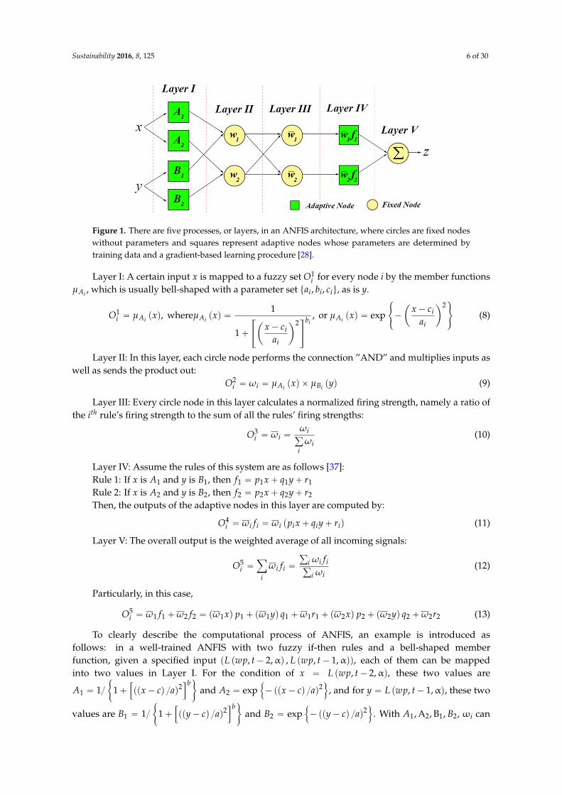
ANFIS is introduced to compensate for the disability of conventional mathematical tools toaddress uncertain systems, such as human knowledge and reasoning processes. Jang [28] restructuredFISs with two contributions: proposing a standard method for transforming ill-defined factors intoidentifiable rules of FIS and using an adaptive network to tune the membership functions. Thisrestructuring yields the ANFIS, which has been validated for its availability in the wind energyarea [35,36]. We assume the system contains two fuzzy if-then rules [37], two inputs (x and y) and oneoutput (z), and the processes of ANFIS are described in Figure 1.
Sustainability 2016, 8, 125 6 of 30
Sustainability 2016, 8, 125 6 of 31
Figure 1. There are five processes, or layers, in an ANFIS architecture, where circles are fixed nodes
without parameters and squares represent adaptive nodes whose parameters are determined by
training data and a gradient‐based learning procedure [28].
Layer I: A certain input is mapped to a fuzzy set 1iO for every node i by the member
functions iA
, which is usually bell‐shaped with a parameter set i i ia ,b ,c , as is y.
1
ii AO x , where 2
1
1
i iA b
i
i
xx c
a
or 2
=i
iA
i
x cx exp
a
(8)
Layer II: In this layer, each circle node performs the connection ”AND” and multiplies inputs as
well as sends the product out:
2
i ii i A BO x y (9)
Layer III: Every circle node in this layer calculates a normalized firing strength, namely a ratio
of the thi rule’s firing strength to the sum of all the rules’ firing strengths:
3 ii i
ii
O
(10)
Layer IV: Assume the rules of this system are as follows [37]:
Rule 1: If x is 1A and y is 1B , then 1 1 1 1f p x q y r
Rule 2: If x is 2A and y is 2B , then 2 2 2 2f p x q y r
Then, the outputs of the adaptive nodes in this layer are computed by:
4i i i i i i iO f p x q y r (11)
Layer V: The overall output is the weighted average of all incoming signals:
5 i iii i i
i ii
fO f
(12)
Particularly, in this case,
51 1 2 2 1 1 1 1 1 1 2 2 2 2 2 2iO f f x p y q r x p y q r (13)
To clearly describe the computational process of ANFIS, an example is introduced as follows: in
a well‐trained ANFIS with two fuzzy if‐then rules and a bell‐shaped member function, given a
x
Figure 1. There are five processes, or layers, in an ANFIS architecture, where circles are fixed nodeswithout parameters and squares represent adaptive nodes whose parameters are determined bytraining data and a gradient-based learning procedure [28].
Layer I: A certain input x is mapped to a fuzzy set O1i for every node i by the member functions
µAi , which is usually bell-shaped with a parameter set tai, bi, ciu, as is y.
O1i “ µAi pxq, whereµAi pxq “
1
1`
«
ˆ
x´ ciai
˙2ffbi
, or µAi pxq “ exp
#
´
ˆ
x´ ciai
˙2+
(8)
Layer II: In this layer, each circle node performs the connection ”AND” and multiplies inputs aswell as sends the product out:
O2i “ ωi “ µAi pxq ˆ µBi pyq (9)
Layer III: Every circle node in this layer calculates a normalized firing strength, namely a ratio ofthe ith rule’s firing strength to the sum of all the rules’ firing strengths:
O3i “ ωi “
ωiř
iωi
(10)
Layer IV: Assume the rules of this system are as follows [37]:Rule 1: If x is A1 and y is B1, then f1 “ p1x` q1y` r1
Rule 2: If x is A2 and y is B2, then f2 “ p2x` q2y` r2
Then, the outputs of the adaptive nodes in this layer are computed by:
O4i “ ωi fi “ ωi ppix` qiy` riq (11)
Layer V: The overall output is the weighted average of all incoming signals:
O5i “
ÿ
i
ωi fi “
ř
i ωi fiř
i ωi(12)
Particularly, in this case,
O5i “ ω1 f1 `ω2 f2 “ pω1xq p1 ` pω1yq q1 `ω1r1 ` pω2xq p2 ` pω2yq q2 `ω2r2 (13)
To clearly describe the computational process of ANFIS, an example is introduced asfollows: in a well-trained ANFIS with two fuzzy if-then rules and a bell-shaped memberfunction, given a specified input pL pwp, t´ 2,αq , L pwp, t´ 1,αqq, each of them can be mappedinto two values in Layer I. For the condition of x “ L pwp, t´ 2,αq, these two values are
A1 “ 1{"
1`”
ppx´ cq {aq2ıb*
and A2 “ exp!
´ppx´ cq {aq2)
, and for y “ L pwp, t´ 1,αq, these two
values are B1 “ 1{"
1`”
ppy´ cq {aq2ıb*
and B2 “ exp!
´ppy´ cq {aq2)
. With A1, A2, B1, B2, ωi can

Sustainability 2016, 8, 125 7 of 30
be computed such that ω1 “ A1 ˆ B1 and ω2 “ A2 ˆ B2. In Layer III, ωi can be computed easily byEquation (10). In Layer IV, based on the two if-then rules, f1 “ p1x` q1y` r1 and f2 “ p2x` q2y` r2
and the output of Layer IV isωi fi. The output of Layer V, which is the output of the ANFIS, is a simplesum of the output of Layer IV, namely L pwp, t,αq “ ω1 f1 `ω2 f2. To achieve a desired input-outputmapping, the parameters are updated according to given training samples and a gradient-basedlearning procedure is described in [28].
2.3.2. Subtractive Clustering Algorithm
Layer I of ANFIS involves determining the membership functions (MFs), and, generally, it is hardfor a visualization technique to reach the necessary precision, especially when the number of rulesexceeds three [38]. Therefore, it is highly desirable that an automatic model identification method berealized by a data set rather than an expert’s experience. Clustering skills are often introduced here,and this paper applies the subtractive clustering algorithm.
For the subtractive clustering method, each data point xi is considered a potential cluster center;then, based on the density of its neighbor points, final clusters are determined by the likelihood ofeach cluster center [39].
For data points txiu in the M-Dimension space, the likelihood Pi of each potential cluster center xiis defined as below:
Pi “
mÿ
j“1
exp
˜
´||xi ´ xj||2
pr{2q2
¸
(14)
where ||xi ´ xj|| denotes the Euclidean distance between xi and its neighbors xj, and r is a positiveconstant defining a neighborhood radius. The first cluster center P˚c1
is chosen as the point c1 whichhas the highest likelihood value. For the next center, the likelihood value is computed after subtractingthe effect of the former cluster center, as follows:
Pi “ Pi ´ P˚c1exp
˜
´||xi ´ xc1||2
pr1{2q2
¸
(15)
where r1 “ η˚r and η˚ is a constant larger than one to avoid cluster centers being in too-closeproximity [40]. Similarly, the second cluster center c2 has a larger likelihood value than the otherpoints. Generally, cluster centers are iteratively selected by Equation (16) until the stopping criteriaare achieved.
ck “ arg maxi
!
Pi
ˇ
ˇ
ˇPi “ Pi ´ P˚ck´1
exp´
´||xi ´ xck´1||2{`
r1{2˘2¯ˇ
ˇ
ˇ
)
(16)
Definition 2.3.1. Given an initial neighborhood radius r ~ U(a, b), a and b are fixed, and theestimation yi of xi by ANFIS with the subtractive clustering method can be defined as below [28]:
yi “ Model pxiq (17)
This map’s Model is defined as
Modelpxi; rq “ ANFISpTrainSet, rq (18)
where TrainSet = {xi, Yi}, and Yi is the actual value of xi.Remark: In Definition 2.3.1, Model(xi;r) is a map from xi to yi and is relative to r, which is a random
variable. When r is a constant, we can express this model simply using Model(xi).
2.4. Firefly Algorithm
The firefly algorithm (FA), developed by Xin-she Tang [29], is enlightened by the natural behaviorsof the firefly. A firefly moves together with other partners because of its tendency to move toward abrighter flash, which is determined by the light intensity of the other fireflies and the distance betweenthem. Assuming three idealized rules are established [29], FA can be summarized as follows.

Sustainability 2016, 8, 125 8 of 30
Definition 2.4.1: I pγq of a firefly is the visible light intensity with γ distance from other fireflies:
I pγq “ I0e´aγ2(19)
where I0 is the light intensity of the firefly itself and a the light absorption coefficient.Definition 2.4.2: β pγq is the attractiveness of a firefly with r distance from other fireflies:
β pγq “ β0e´aγ2(20)
where β pγq represents the maximum attractiveness.Definition 2.4.3: Firefly i will be attracted by a brighter firefly j with movement determined by
xi pt` 1q “ xi ptq ` β`
xj ptq ´ xi ptq˘
` δ
ˆ
rand´12
˙
(21)
where δ is the randomization parameter.Based on the rules and definitions above, FA can be summarized in Algorithm 1.
Algorithm 1. Firefly Algorithm.
Input: x “ px1, x2, . . . , xdqT , Objective function: f pxq
Generate initial population of fireflies xi pi “ 1, 2, . . . , nq
Sustainability 2016, 8, 125 8 of 31
i iy Model x (17)
This map’s Model is defined as
( ; ) (TrainSet, )iModel x r ANFIS r (18)
where TrainSet = {xi, Yi}, and Yi is the actual value of xi.
Remark: In Definition 2.3.1, Model(xi;r) is a map from xi to yi and is relative to r, which is a random
variable. When r is a constant, we can express this model simply using Model(xi).
2.4. Firefly Algorithm
The firefly algorithm (FA), developed by Xin‐she Tang [29], is enlightened by the natural
behaviors of the firefly. A firefly moves together with other partners because of its tendency to move
toward a brighter flash, which is determined by the light intensity of the other fireflies and the
distance between them. Assuming three idealized rules are established [29], FA can be summarized
as follows.
Definition 2.4.1: I of a firefly is the visible light intensity with distance from other
fireflies:
2
0aI I e (19)
where 0I is the light intensity of the firefly itself and a the light absorption coefficient. Definition 2.4.2: is the attractiveness of a firefly with r distance from other fireflies:
2
0ae (20)
where represents the maximum attractiveness.
Definition 2.4.3: Firefly i will be attracted by a brighter firefly j with movement determined by
11
2i i j ix t x t x t x t rand
(21)
where δ is the randomization parameter.
Based on the rules and definitions above, FA can be summarized in Algorithm 1.
Algorithm 1. Firefly Algorithm.
Input: 1 2
T
dx ,x , ,x Kx , Objective function: f x
Generate initial population of fireflies 1 2i i , , ,n Kx
While t MaxIteration
For 1i : n
For 1j : i
If j iI I
11
2i i j ix t x t x t x t rand
Else
1i ix t x t
End If
End For
End While
3. Introduction to the Proposed Model
Let N be a set of positive integers, and suppose that W = (wp1, wp2, . . . , wpn) , which is the meanwind power series, and wpi P [0, C], where n P N and C denotes the installed capacity of the wind farm(it should be clarified that this paper only collects wind power data and there is no other additionaldata used, which indicates that the input data of the models is only wind power data). The main stepsof the proposed model are as demonstrated below.
Step 1. Divide W into Wtrain = (wp1, wp2, . . . , wpm) and Wtest = (wpm`1, wp2, . . . , wpn), and theyboth satisfy
Wtrainď
Wtest “ W and Wtrainč
Wtest “ ∅ (22)
Step 2. According to Definition 2.2.2, let
Wstrain “ SSApWtrain, 10, 4q (23)
Step 3. Let d, nt PN, X Ď Rd be the input space constructed by elements in Wtrain and Y Ď R bethe output space constructed by elements in Wstrain. Let
TA “ pxi, yiqnti“1 (24)
where TA is a family of random samples in which xi P X and yi P Y.

Sustainability 2016, 8, 125 9 of 30
Step 4. Let ntr, nvd P [1, nt)Ă N, and generate nvd random numbers ri (i = 1, 2, . . . , nvd) that obeya normalized Gaussian distribution
Sustainability 2016, 8, 125 9 of 31
3. Introduction to the Proposed Model
Let N be a set of positive integers, and suppose that W = (wp1, wp2, …, wpn) , which is the mean
wind power series, and wpi ∈ [0, C], where n ∈ N and C denotes the installed capacity of the wind
farm (it should be clarified that this paper only collects wind power data and there is no other
additional data used, which indicates that the input data of the models is only wind power data). The
main steps of the proposed model are as demonstrated below.
Step 1. Divide W into Wtrain = (wp1, wp2, …, wpm) and Wtest = (wpm+1, wp2, …, wpn), and they both satisfy
and train test train testW W W W W U I (22)
Step 2. According to Definition 2.2.2, let
( ,10,4)train trainWs SSAW (23)
Step 3. Let d, nt∈N, X⊆ R be the input space constructed by elements in Wtrain and Y ⊆R be the output space constructed by elements in Wstrain. Let
TA ( , )1
ntx yi i i
(24)
where TA is a family of random samples in which xi ∈X and yi ∈Y. Step 4. Let ntr, nvd∈[1, nt)⊂N, and generate nvd random numbers ri (i = 1, 2, …, nvd) that obey
a normalized Gaussian distribution Ɲ(0,1). Let
, 1, 2,..., Nvd i iI nt r r i nvd (25)
Thus, we have
Vd ( , )vdi i i Ix y (26)
and
TRN ( , ) TA [1, ] and i i vdx y i nt i I = (27)
Step 5. Let α ∈(0, 1] be a parameter to calculate the upper and lower bounds of interval forecasts,
and we have
Vd_U( ) ( , ) ( , ) Vdi i i ix C y x y (28)
Vd_L( ) ( , ) ( , ) Vdi i i ix C y x y (29)
and
TRN_U( ) ( , ) ( , ) TRNi i i ix C y x y (30)
TRN_L( ) ( , ) ( , ) TRNi i i ix C y x y (31)
Step 6. Adjust yi of Vd_U, Vd_L, TRN_U and TRN_L using the following equation:
Vd_U,Vd_L,TRN_U
0, 0
1and TR
,N_L,
,
i
ii
i
i
y
y Cy
yotherwi
y
seC
(32)
(0,1). Let
Ivd “ ttntˆ riu |ri, i “ 1, 2, . . . , nvdu Ă N (25)
Thus, we have
Vd “ pxi, yiqiPIvd(26)
and
TRN “ tpxi, yiq P TA |i P r1, nts and i R Ivd u (27)
Step 5. Let α P (0, 1] be a parameter to calculate the upper and lower bounds of interval forecasts,and we have
Vd_Upαq “ tpxi, αˆ C` yiq |pxi, yiq P Vdu (28)
Vd_Lpαq “ tpxi,´αˆ C` yiq |pxi, yiq P Vdu (29)
and
TRN_Upαq “ tpxi, αˆ C` yiq |pxi, yiq P TRNu (30)
TRN_Lpαq “ tpxi,´αˆ C` yiq |pxi, yiq P TRNu (31)
Step 6. Adjust yi of Vd_U, Vd_L, TRN_U and TRN_L using the following equation:
yi “
$
’
’
’
&
’
’
’
%
0, yi ă 0
1, yi ą CyiC
, otherwise
, yi P Vd_U, Vd_L, TRN_U and TRN _L (32)
Step 7. According to Definition 2.3.1, build and train two basic ANFISs with TRN_U, TRN_L andr ~ U(0.03,0.3), which is a neighborhood radius of the subtractive clustering method, and we expressboth of them by
Model_Upxi; rq “ ANFISpTRN_U, rq (33)
andModel_Lpxi; rq “ ANFISpTRN_L, rq (34)
where Model_U and Model_L are maps from X to Y, and their parameters are relative with r.Step 8. Generate a loss function:
Jprq “nvdÿ
i“1
ˆ
b
pModel_UpxUi ; rq ´ yU
i q2`
b
pModel_LpxLi ; rq ´ yL
i q2˙
(35)
where pxUi , yU
i q P Vd_U and pxLi , yL
i q P Vd_L.
Step 9. Let the objective function of FA be
Minr
Jprq (36)
where r ~ U(0.03, 0.3), and denote the best r obtained by this objective function by rbest P [0.03,0.3].Step 10. Obtain the IFASF model and express it by
IFASF_Upxiq “ ANFISpTRN_U, rbestq (37)
and
IFASF_Lpxiq “ ANFISpTRN_L, rbestq (38)

Sustainability 2016, 8, 125 10 of 30
Remark: Step 1 to Step 10 specifically demonstrate IFASF using a mathematical process, and theyshow how to utilize one wind power time series to train the IFASF and obtain an upper bound andlower bound. Figure 2 shows the flowchart of IFASF with a specific sample.Sustainability 2016, 8, 125 11 of 31
Figure 2. Flowchart of the developed model with a specific sample.
4. Numerical Results and Analysis
In this section, detailed forecasting results and corresponding analyses will be demonstrated by
tables and figures, and comparisons between other models will also be specifically illustrated.
4.1. Data Collections, Forecasting Principles and Parameter Settings
We collected wind power data from three different wind farms (denoted by W1, W2 and W3) in
Gansu Province in 2013 and randomly selected 25 weeks of data (175 days from each wind farm) to
validate the effectiveness of the developed model. The main forecasting principles are demonstrated
as follows.
Two previous wind power points of the forecasting point were used to construct input spaces
of a basic ANFIS.
Training samples of the IFASF were constructed for the week to be validated using the previous
60 days of wind power data.
The proposed model was re‐trained after it had provided seven days of forecasting results.
Parameters were set as follows: η and μ of CWC (the definition of CWC and its parameters are
listed in the Appendix) of 0.5 and 75%, respectively.
Figure 2. Flowchart of the developed model with a specific sample.
4. Numerical Results and Analysis
In this section, detailed forecasting results and corresponding analyses will be demonstrated bytables and figures, and comparisons between other models will also be specifically illustrated.
4.1. Data Collections, Forecasting Principles and Parameter Settings
We collected wind power data from three different wind farms (denoted by W1, W2 and W3) inGansu Province in 2013 and randomly selected 25 weeks of data (175 days from each wind farm) tovalidate the effectiveness of the developed model. The main forecasting principles are demonstratedas follows.
‚ Two previous wind power points of the forecasting point were used to construct input spaces of abasic ANFIS.
‚ Training samples of the IFASF were constructed for the week to be validated using the previous60 days of wind power data.
‚ The proposed model was re-trained after it had provided seven days of forecasting results.
Parameters were set as follows: η and µ of CWC (the definition of CWC and its parameters arelisted in the Appendix) of 0.5 and 75%, respectively.

Sustainability 2016, 8, 125 11 of 30
4.2. Interval Forecasting Results
For the purpose of testing the forecasting effectiveness of each model, this paper preparesfive experiments with data from three different wind farms to illustrate each model’s forecastingconsequence and the priority of the developed model.
4.2.1. Experiment I
This experiment shows W1’s interval forecasting effectiveness of ANFIS, ANFIS-SSA and IFASF,which is evaluated by IFCP and IFNAW (the definition of IFCP, IFNAW and its parameters are listedin the Appendix) in Table 2. A 70% interval forecast is more meaningful than other interval forecastsbecause IFCP of the 70% interval forecast is higher than that of the 80% and 90% interval forecasts,indicating that the mean wind power is unstable data and it is difficult to forecast its interval whichcovers the actual values. Although the interval of average wind power data is hard to forecast,ANFIS-SSA and IFASF still give satisfactory results because their IFCPs are more than 70% when usedto forecast a 70% interval of wind power. Alternately, ANFIS only has a 65.14% successful coveragepercentage in the same situation, which suggests that the method developed by SSA and FA indeedimproves the coverage percentage. From the average values of each column, IFCPs of IFASF are 40%,62.29% and 76%, which are higher than the 37.14%, 56.57% and 72% obtained with ANFIS-SSA andthe 30.29%, 52% and 65.14% obtained with ANFIS. For the IFNAW criteria, IFASF also outperformsother models when forecasting the 70% wind power interval. From the perspective of the numberof time that each method reaches a 100% coverage percentage, ANFIS has one week in which theIFCP is 100%, the IFCP of ANFIS-SSA peaks at 100% five times, and the developed model, IFASF, haseight weeks in which the forecasting interval covers all of the actual mean wind power points, whichshows that IFASF is a better model to calculate wind power points’ upper bounds and lower bounds.Specifically, the ANFIS model obtains the highest IFCP when forecasting the 70% interval in week11 and the lowest IFCP in week 2 for the 90% interval forecast. Similarly, the forecasting results inweek 2 of ANFIS-SSA are also invalidated when they are used to calculate the 90% upper and lowerbounds for wind power points. The IFCP of the model developed by SSA peaks at 100% five timeswhen forecasting the 80% interval in week 25 and the 70% interval in weeks 13, 17, 24 and 25. For theIFASF model, its IFCP peaks at 100% eight times: in week 9 for the 70% interval forecast, week 11 forthe 70% interval forecast, week 13 for the 80% and 70% interval forecasts, week 17 for the 70% intervalforecast, week 24 for the 70% interval forecast and week 25 for the 80% and 70% interval forecasts.Additionally, the developed model obtains the worst IFCP when forecasting the 90% interval of week 2.To illustrate the information in this table, Figure 3 is constructed to show the merits of the developedmodel. In Figure 3a, the IFCPs are divided into three categories, which are ranges from 0% to 50%,50% to 80% and 80% to 100%, and it is obvious that the IFCPs of IFASF belong to (80%~100%) 12 times,which are the highest among these three models, and they belong to (50%~80%) and (0%~50%) 10 timesand three times, respectively, which are the lowest among ANFIS, ANFIS-SSA and IFASF (see thetable in the sub-figure of Figure 3). Figure 3b–d are histograms of the IFCPs of the three models, andthe right portion of the IFCP axis indicates a higher IFCP. Thus, the IFASF model’s IFCPs are higherthan those of the other models, indicating that SSA and FA actually improve the interval forecastingability of ANFIS and show a good pre-process and optimal effectiveness for randomly selected weeks.Figure 3e,f illustrate the context of Table 2 and they also show that the proposed model has a goodperformance for 70%, 80% and 90% interval forecasts.

Sustainability 2016, 8, 125 12 of 30
Sustainability 2016, 8, 125 13 of 31
Figure 3. Histograms and plots of the main results of the interval forecast of 25 weeks in W1. Figure 3. Histograms and plots of the main results of the interval forecast of 25 weeks in W1.

Sustainability 2016, 8, 125 13 of 30
Table 2. Main interval forecasting results of ANFIS, ANFIS-SSA and IFASF in W1.
Weeks
ANFIS ANFIS-SSA IFASF
IFCP (%) IFNAW (%) IFCP (%) IFNAW (%) IFCP (%) IFNAW (%)
90.00% 80.00% 70.00% 90.00% 80.00% 70.00% 90.00% 80.00% 70.00% 90.00% 80.00% 70.00% 90.00% 80.00% 70.00% 90.00% 80.00% 70.00%
1 42.86 85.71 85.71 105.07 275.77 393.68 71.43 57.14 85.71 109.43 147.66 335.51 85.71 85.71 71.43 191.02 287.31 386.502 0.00 14.29 42.86 15.81 31.36 43.50 0.00 57.14 71.43 12.48 35.00 51.61 0.00 42.86 71.43 25.42 43.16 58.683 57.14 85.71 85.71 267.57 465.26 619.34 57.14 85.71 85.71 155.64 411.33 514.84 71.43 85.71 85.71 252.09 465.03 509.184 14.29 14.29 14.29 26.83 46.57 67.54 42.86 42.86 28.57 16.32 38.33 64.97 14.29 57.14 28.57 23.86 70.06 75.065 28.57 57.14 57.14 31.22 64.51 92.32 28.57 57.14 85.71 34.81 77.42 119.98 71.43 71.43 85.71 39.74 71.52 97.176 42.86 57.14 57.14 53.53 92.26 134.44 28.57 57.14 85.71 51.26 114.86 178.47 57.14 71.43 85.71 60.74 107.38 150.587 0.00 42.86 57.14 24.30 40.76 56.62 14.29 42.86 42.86 13.86 51.19 78.55 0.00 0.00 57.14 22.36 42.35 62.998 14.29 71.43 85.71 61.09 116.99 168.30 14.29 14.29 71.43 61.03 92.08 137.46 28.57 71.43 85.71 71.34 130.05 160.089 42.86 42.86 57.14 29.50 58.16 94.26 57.14 57.14 71.43 65.33 81.89 111.91 28.57 42.86 100.00 39.50 76.20 108.2110 14.29 28.57 85.71 30.89 56.08 90.33 28.57 28.57 71.43 41.52 97.75 138.11 28.57 28.57 42.86 25.73 47.66 75.2711 57.14 42.86 100.00 41.80 78.32 122.65 57.14 42.86 85.71 29.16 79.54 137.64 28.57 85.71 100.00 60.37 111.30 149.2312 14.29 28.57 57.14 13.77 30.60 50.11 57.14 57.14 57.14 27.29 49.66 64.96 14.29 42.86 42.86 14.25 28.58 43.0213 42.86 71.43 85.71 88.70 104.78 184.63 42.86 85.71 100.00 76.56 139.94 191.12 57.14 100.00 100.00 64.04 116.80 161.4614 57.14 57.14 57.14 16.77 42.92 54.18 14.29 71.43 85.71 34.46 61.51 87.81 71.43 85.71 85.71 31.25 72.51 94.2615 28.57 57.14 57.14 35.02 64.42 95.95 42.86 42.86 57.14 43.36 76.63 102.96 42.86 57.14 71.43 34.60 73.86 107.2316 14.29 57.14 57.14 40.11 65.05 89.27 28.57 57.14 71.43 47.49 87.24 118.71 28.57 71.43 71.43 38.69 80.90 107.8317 28.57 71.43 57.14 123.65 123.65 123.65 57.14 85.71 100.00 95.70 216.81 213.21 0.00 57.14 100.00 76.35 138.55 197.4718 57.14 42.86 71.43 36.76 61.57 88.82 14.29 42.86 28.57 32.42 57.29 82.20 14.29 42.86 71.43 38.42 58.40 115.1219 28.57 71.43 85.71 42.39 79.05 111.73 28.57 28.57 42.86 35.56 70.96 98.38 57.14 57.14 71.43 52.12 75.97 108.2020 28.57 28.57 57.14 23.50 46.81 76.41 28.57 57.14 71.43 46.04 70.74 94.32 57.14 71.43 71.43 28.20 55.17 86.4521 14.29 42.86 42.86 23.05 44.76 63.10 42.86 57.14 71.43 23.66 46.45 66.92 28.57 42.86 57.14 23.31 47.81 79.5522 28.57 57.14 57.14 71.18 107.62 140.72 28.57 57.14 71.43 37.50 73.17 102.43 42.86 57.14 85.71 42.04 80.83 123.2223 14.29 42.86 57.14 59.15 84.89 109.01 28.57 57.14 57.14 30.59 57.02 83.23 28.57 57.14 57.14 32.27 68.70 77.8724 57.14 71.43 85.71 246.94 279.60 309.60 71.43 71.43 100.00 51.82 80.93 123.90 71.43 71.43 100.00 51.34 90.52 122.6525 28.57 57.14 71.43 40.44 97.40 188.15 42.86 100.00 100.00 75.54 154.32 209.33 71.43 100.00 100.00 88.92 162.63 219.78
Std. 18.13 19.73 18.93 64.95 98.42 127.65 18.90 19.55 20.82 32.69 77.29 99.79 25.75 22.92 20.08 53.66 91.66 103.63Average 30.29 52.00 65.14 61.96 102.37 142.73 37.14 56.57 72.00 49.95 98.79 140.34 40.00 62.29 76.00 57.12 104.13 139.08

Sustainability 2016, 8, 125 14 of 30
4.2.2. Experiment II
In this experiment, interval forecasting results of ARIMA, BPNN, ELM, ARIMA-SSA, BPNN-SSA,ELM-SSA, ANFIS, ANFIS-SSA and IFASF will be demonstrated and compared in W1. The ARIMAmodel is an extension of the regular ARMA model and involves three essential parts of auto-regression,moving average and integration in order to model the serial correlations of a stochastic process [41].ELM is a single hidden-layer feedforward neural network, which randomly chooses the input weightsand analytically determines the output weights [42]. As one of the famous machine learning algorithms,BPNN is also employed as a benchmarking comparison model [43]. The ARIMA-SSA, BPNN-SSAand ELM-SSA models all use SSA pre-processed data to train ARIMA, BPNN and ELM, respectively(when testing the effectiveness of BPNN and ELM, they both use actual data to construct the inputspace). Table 3 shows the main interval forecasting results of nine models by three criteria, and CWC’sparameters are mentioned in Section 4.1. From this table, IFASF obviously has a higher mean IFCPthan the other models, and only the developed model meets the 75% standard set in the CWC criteria,which is a combined index to evaluate the effectiveness of interval forecasts. Additionally, for theCWC criteria, IFASF has the lowest values for 70% and 80% interval forecasts. From the perspective ofthe interval forecasts’ utility, 90% interval forecasts are invalidated for the reason that the highest IFCPof these models is 40%, which is far from the standard 75% (possibly because of the stochastic natureof wind and wind power). Thus, we will mainly discuss each model’s effectiveness when forecasting70% and 80% intervals in this section. For ARIMA and ARIMA-SSA models, the highest IFCP peaks at61.14% using ARIMA pre-processed by SSA for 70% interval forecasts, and the lowest CWC is 860.18,which appears when forecasting an 80% interval using ARIMA-SSA. From the boxplot of ARIMA andARIMA-SSA’s interval forecasts shown in Figure 4, the SSA method develops the original ARIMAto obtain a better forecasting performance than the original one (CWC provides the main criteria toevaluate the model’s effectiveness). The BPNN model is a classical artificial neuron network (ANN)and has been used to solve many forecasting problems. In this paper, BPNN utilizes historical data totrain its parameters and directly obtains the upper bounds and lower bounds.
Sustainability 2016, 8, 125 14 of 31
4.2.2. Experiment II
In this experiment, interval forecasting results of ARIMA, BPNN, ELM, ARIMA‐SSA, BPNN‐SSA,
ELM‐SSA, ANFIS, ANFIS‐SSA and IFASF will be demonstrated and compared in W1. The ARIMA
model is an extension of the regular ARMA model and involves three essential parts of auto‐
regression, moving average and integration in order to model the serial correlations of a stochastic
process [41]. ELM is a single hidden‐layer feedforward neural network, which randomly chooses the
input weights and analytically determines the output weights [42]. As one of the famous machine
learning algorithms, BPNN is also employed as a benchmarking comparison model [43]. The
ARIMA‐SSA, BPNN‐SSA and ELM‐SSA models all use SSA pre‐processed data to train ARIMA,
BPNN and ELM, respectively (when testing the effectiveness of BPNN and ELM, they both use actual
data to construct the input space). Table 3 shows the main interval forecasting results of nine models
by three criteria, and CWC’s parameters are mentioned in Section 4.1. From this table, IFASF
obviously has a higher mean IFCP than the other models, and only the developed model meets the
75% standard set in the CWC criteria, which is a combined index to evaluate the effectiveness of
interval forecasts. Additionally, for the CWC criteria, IFASF has the lowest values for 70% and 80%
interval forecasts. From the perspective of the interval forecasts’ utility, 90% interval forecasts are
invalidated for the reason that the highest IFCP of these models is 40%, which is far from the standard
75% (possibly because of the stochastic nature of wind and wind power). Thus, we will mainly
discuss each model’s effectiveness when forecasting 70% and 80% intervals in this section. For
ARIMA and ARIMA‐SSA models, the highest IFCP peaks at 61.14% using ARIMA pre‐processed by
SSA for 70% interval forecasts, and the lowest CWC is 860.18, which appears when forecasting an
80% interval using ARIMA‐SSA. From the boxplot of ARIMA and ARIMA‐SSA’s interval forecasts
shown in Figure 4, the SSA method develops the original ARIMA to obtain a better forecasting
performance than the original one (CWC provides the main criteria to evaluate the model’s
effectiveness). The BPNN model is a classical artificial neuron network (ANN) and has been used to
solve many forecasting problems. In this paper, BPNN utilizes historical data to train its parameters
and directly obtains the upper bounds and lower bounds.
Figure 4. Boxplot of the results of ARIMA and ARIMA‐SSA by three criteria in W1 (for the purpose
of convenient comparisons among these models, the CWC axis is limited below 2000 and there are
many points that are not shown in the CWC part of Figure 4).
Figure 4. Boxplot of the results of ARIMA and ARIMA-SSA by three criteria in W1 (for the purpose ofconvenient comparisons among these models, the CWC axis is limited below 2000 and there are manypoints that are not shown in the CWC part of Figure 4).
Sustainability 2016, 8, 125 15 of 30
Table 3. Main interval forecasting results of the nine models in W1.
Model
Criteria
Mean IFCP (%) Mean IFNAW (%) Mean CWC (%)
90.00% 80.00% 70.00% 90.00% 80.00% 70.00% 90.00% 80.00% 70.00%
ARIMA 30.29 52.00 60.57 47.21 101.74 143.35 806.61 1443.84 1922.82BPNN 29.71 53.71 57.14 53.58 102.82 142.30 569.97 659.20 597.81ELM 29.14 49.71 62.86 53.90 99.08 138.60 590.70 464.48 410.68
ANFIS 30.29 52.00 65.14 61.96 102.37 142.73 648.38 372.92 358.90ARIMA-SSA 27.43 50.29 61.14 47.09 87.33 124.99 918.05 860.18 1402.35BPNN-SSA 36.57 50.29 71.43 54.57 93.93 133.92 447.79 430.42 309.64ELM-SSA 36.00 54.29 71.43 52.46 93.62 132.74 431.81 380.32 483.80
ANFIS-SSA 37.14 56.57 72.00 49.95 98.79 140.34 415.39 384.66 293.10IFASF 40.00 62.29 76.00 57.12 104.13 139.08 508.16 321.53 261.04
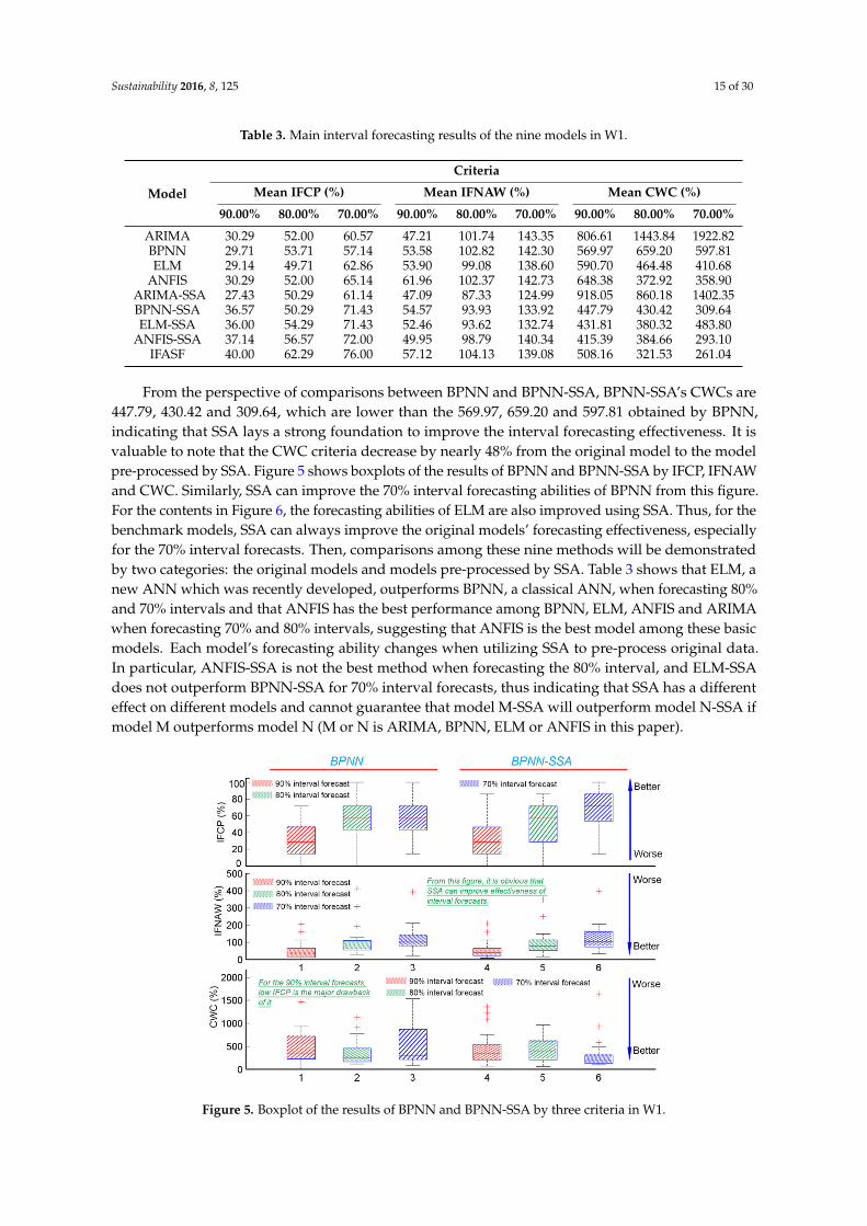
From the perspective of comparisons between BPNN and BPNN-SSA, BPNN-SSA’s CWCs are447.79, 430.42 and 309.64, which are lower than the 569.97, 659.20 and 597.81 obtained by BPNN,indicating that SSA lays a strong foundation to improve the interval forecasting effectiveness. It isvaluable to note that the CWC criteria decrease by nearly 48% from the original model to the modelpre-processed by SSA. Figure 5 shows boxplots of the results of BPNN and BPNN-SSA by IFCP, IFNAWand CWC. Similarly, SSA can improve the 70% interval forecasting abilities of BPNN from this figure.For the contents in Figure 6, the forecasting abilities of ELM are also improved using SSA. Thus, for thebenchmark models, SSA can always improve the original models’ forecasting effectiveness, especiallyfor the 70% interval forecasts. Then, comparisons among these nine methods will be demonstratedby two categories: the original models and models pre-processed by SSA. Table 3 shows that ELM, anew ANN which was recently developed, outperforms BPNN, a classical ANN, when forecasting 80%and 70% intervals and that ANFIS has the best performance among BPNN, ELM, ANFIS and ARIMAwhen forecasting 70% and 80% intervals, suggesting that ANFIS is the best model among these basicmodels. Each model’s forecasting ability changes when utilizing SSA to pre-process original data.In particular, ANFIS-SSA is not the best method when forecasting the 80% interval, and ELM-SSAdoes not outperform BPNN-SSA for 70% interval forecasts, thus indicating that SSA has a differenteffect on different models and cannot guarantee that model M-SSA will outperform model N-SSA ifmodel M outperforms model N (M or N is ARIMA, BPNN, ELM or ANFIS in this paper).
Sustainability 2016, 8, 125 15 of 31
Table 3. Main interval forecasting results of the nine models in W1.
Model
Criteria
Mean IFCP (%) Mean IFNAW (%) Mean CWC (%)
90.00% 80.00% 70.00% 90.00% 80.00% 70.00% 90.00% 80.00% 70.00%
ARIMA 30.29 52.00 60.57 47.21 101.74 143.35 806.61 1443.84 1922.82
BPNN 29.71 53.71 57.14 53.58 102.82 142.30 569.97 659.20 597.81
ELM 29.14 49.71 62.86 53.90 99.08 138.60 590.70 464.48 410.68
ANFIS 30.29 52.00 65.14 61.96 102.37 142.73 648.38 372.92 358.90
ARIMA‐SSA 27.43 50.29 61.14 47.09 87.33 124.99 918.05 860.18 1402.35
BPNN‐SSA 36.57 50.29 71.43 54.57 93.93 133.92 447.79 430.42 309.64
ELM‐SSA 36.00 54.29 71.43 52.46 93.62 132.74 431.81 380.32 483.80
ANFIS‐SSA 37.14 56.57 72.00 49.95 98.79 140.34 415.39 384.66 293.10
IFASF 40.00 62.29 76.00 57.12 104.13 139.08 508.16 321.53 261.04
From the perspective of comparisons between BPNN and BPNN‐SSA, BPNN‐SSA’s CWCs are
447.79, 430.42 and 309.64, which are lower than the 569.97, 659.20 and 597.81 obtained by BPNN,
indicating that SSA lays a strong foundation to improve the interval forecasting effectiveness. It is
valuable to note that the CWC criteria decrease by nearly 48% from the original model to the model
pre‐processed by SSA. Figure 5 shows boxplots of the results of BPNN and BPNN‐SSA by IFCP,
IFNAW and CWC. Similarly, SSA can improve the 70% interval forecasting abilities of BPNN from
this figure. For the contents in Figure 6, the forecasting abilities of ELM are also improved using SSA.
Thus, for the benchmark models, SSA can always improve the original models’ forecasting
effectiveness, especially for the 70% interval forecasts. Then, comparisons among these nine methods
will be demonstrated by two categories: the original models and models pre‐processed by SSA.
Table 3 shows that ELM, a new ANN which was recently developed, outperforms BPNN, a classical
ANN, when forecasting 80% and 70% intervals and that ANFIS has the best performance among
BPNN, ELM, ANFIS and ARIMA when forecasting 70% and 80% intervals, suggesting that ANFIS is
the best model among these basic models. Each model’s forecasting ability changes when utilizing
SSA to pre‐process original data. In particular, ANFIS‐SSA is not the best method when forecasting
the 80% interval, and ELM‐SSA does not outperform BPNN‐SSA for 70% interval forecasts, thus
indicating that SSA has a different effect on different models and cannot guarantee that model
M‐SSA will outperform model N‐SSA if model M outperforms model N (M or N is ARIMA, BPNN,
ELM or ANFIS in this paper).
Figure 5. Boxplot of the results of BPNN and BPNN‐SSA by three criteria in W1. Figure 5. Boxplot of the results of BPNN and BPNN-SSA by three criteria in W1.

Sustainability 2016, 8, 125 16 of 30
Sustainability 2016, 8, 125 16 of 31
Figure 6. Boxplot of the results of ELM and ELM‐SSA by three criteria in W1.
However, no matter which model (basic models or models pre‐processed by SSA) is considered,
the IFASF model is still the best interval forecasting model because its IFCP is closer to the standard
IFCP of 75% than the IFCPs of the other models. In Figure 7, which presents the boxplot of each model
when forecasting 70% and 80% intervals, the blue line represents the 75th percentile of CWC of 80%
interval forecasts and the red line represents the 75th percentile of CWC of 70% interval forecasts.
It is obvious that the red line’s points are almost lower than those of the blue line, suggesting that
70% interval forecasts have better performance than 80% interval forecasts. From the perspective of
the models’ forecasting effectiveness, IFASF apparently outperforms other models no matter which
criteria are considered to evaluate interval forecasts (such as the median of CWC, the 75th percentile
of CWC or the average value of CWC). Thus, from the above analysis of forecasting results, the
developed model, IFASF, is the best interval forecasting model for mean wind power points.
Figure 7. Boxplot of each model when forecasting 70% and 80% intervals in W1.
Figure 6. Boxplot of the results of ELM and ELM-SSA by three criteria in W1.
However, no matter which model (basic models or models pre-processed by SSA) is considered,the IFASF model is still the best interval forecasting model because its IFCP is closer to the standardIFCP of 75% than the IFCPs of the other models. In Figure 7, which presents the boxplot of each modelwhen forecasting 70% and 80% intervals, the blue line represents the 75th percentile of CWC of 80%interval forecasts and the red line represents the 75th percentile of CWC of 70% interval forecasts. It isobvious that the red line’s points are almost lower than those of the blue line, suggesting that 70%interval forecasts have better performance than 80% interval forecasts. From the perspective of themodels’ forecasting effectiveness, IFASF apparently outperforms other models no matter which criteriaare considered to evaluate interval forecasts (such as the median of CWC, the 75th percentile of CWCor the average value of CWC). Thus, from the above analysis of forecasting results, the developedmodel, IFASF, is the best interval forecasting model for mean wind power points.
Sustainability 2016, 8, 125 16 of 31
Figure 6. Boxplot of the results of ELM and ELM‐SSA by three criteria in W1.
However, no matter which model (basic models or models pre‐processed by SSA) is considered,
the IFASF model is still the best interval forecasting model because its IFCP is closer to the standard
IFCP of 75% than the IFCPs of the other models. In Figure 7, which presents the boxplot of each model
when forecasting 70% and 80% intervals, the blue line represents the 75th percentile of CWC of 80%
interval forecasts and the red line represents the 75th percentile of CWC of 70% interval forecasts.
It is obvious that the red line’s points are almost lower than those of the blue line, suggesting that
70% interval forecasts have better performance than 80% interval forecasts. From the perspective of
the models’ forecasting effectiveness, IFASF apparently outperforms other models no matter which
criteria are considered to evaluate interval forecasts (such as the median of CWC, the 75th percentile
of CWC or the average value of CWC). Thus, from the above analysis of forecasting results, the
developed model, IFASF, is the best interval forecasting model for mean wind power points.
Figure 7. Boxplot of each model when forecasting 70% and 80% intervals in W1.
Figure 7. Boxplot of each model when forecasting 70% and 80% intervals in W1.

Sustainability 2016, 8, 125 17 of 30
4.2.3. Experiment III
Initially, this experiment will show the interval forecasting effectiveness of ANFIS, ANFIS-SSAand IFASF in W2, which are evaluated by IFCP and IFNAW in Table 4. It is apparent that the 70%interval forecast is more meaningful than the other interval forecasts because the IFCP of the 70%interval forecast is higher than that of the 80% and 90% interval forecasts, which are similar to theresults obtained in W1. ANFIS-SSA and IFASF provide satisfactory results because their IFCPs aremore than 70% when they are used to forecast 70% intervals of wind power. However, ANFIS hasonly a 63.43% successful coverage percentage in the same situation, which means that SSA and FAplay important roles in improving the coverage percentage. From the average values of each column,the IFCPs of IFASF are higher than those of ANFIS-SSA and ANFIS when forecasting 70% and 80%intervals. For the IFNAW criteria, IFASF also outperforms other models when forecasting 70% and80% wind power intervals. From the perspective of high coverage percentage, ANFIS has nine weekswhose IFCPs are over 80%, the IFCP of ANFIS-SSA is more than 80% 22 times and the developedmodel, IFASF, also has 22 weeks in which the forecasting interval covers 80% of the actual mean windpower points, which shows that ANFIS-SSA and IFASF are better models to calculate the wind powerpoints’ upper bounds and lower bounds. Specifically, if IFCPs are divided into three categories thatrange from 0% to 50%, 50% to 80% and 80% to 100%, then it will be obvious that the IFCPs of IFASFbelong to (80%~100%) 22 times, which is higher than those of ANFIS, and to (50%~80%) and (0%~50%)31 and 22 times, respectively. In Figure 8a, the red and blue lines divide this figure into three parts,which represent the intervals (80%–100%), (50%–80%) and (0%–50%) of IFCP. Figure 8b,c illustratethe context of Table 4 and they indicate that the proposed model has higher FICPs than ANFIS andANFIS-SSA have. From this figure and Table 4, it can be observed that IFASF outperforms ANFIS-SSAmainly because when their IFCPs belong to (0%–50%), the IFCPs of the developed model are higherthan those of ANFIS-SSA, and IFASF outperforms ANFIS because IFASF has more points whose IFCPsare over 80% than ANFIS does.
Sustainability 2016, 8, 125 17 of 31
4.2.3. Experiment III
Initially, this experiment will show the interval forecasting effectiveness of ANFIS, ANFIS‐SSA
and IFASF in W2, which are evaluated by IFCP and IFNAW in Table 4. It is apparent that the 70%
interval forecast is more meaningful than the other interval forecasts because the IFCP of the 70%
interval forecast is higher than that of the 80% and 90% interval forecasts, which are similar to the
results obtained in W1. ANFIS‐SSA and IFASF provide satisfactory results because their IFCPs are
more than 70% when they are used to forecast 70% intervals of wind power. However, ANFIS has
only a 63.43% successful coverage percentage in the same situation, which means that SSA and FA
play important roles in improving the coverage percentage. From the average values of each column,
the IFCPs of IFASF are higher than those of ANFIS‐SSA and ANFIS when forecasting 70% and 80%
intervals. For the IFNAW criteria, IFASF also outperforms other models when forecasting 70% and
80% wind power intervals. From the perspective of high coverage percentage, ANFIS has nine weeks
whose IFCPs are over 80%, the IFCP of ANFIS‐SSA is more than 80% 22 times and the developed
model, IFASF, also has 22 weeks in which the forecasting interval covers 80% of the actual mean wind
power points, which shows that ANFIS‐SSA and IFASF are better models to calculate the wind power
points’ upper bounds and lower bounds. Specifically, if IFCPs are divided into three categories that
range from 0% to 50%, 50% to 80% and 80% to 100%, then it will be obvious that the IFCPs of IFASF
belong to (80%~100%) 22 times, which is higher than those of ANFIS, and to (50%~80%) and (0%~50%)
31 and 22 times, respectively. In Figure 8a, the red and blue lines divide this figure into three parts,
which represent the intervals (80%–100%), (50%–80%) and (0%–50%) of IFCP. Figure 8b,c illustrate the
context of Table 4 and they indicate that the proposed model has higher FICPs than ANFIS and
ANFIS‐SSA have. From this figure and Table 4, it can be observed that IFASF outperforms ANFIS‐
SSA mainly because when their IFCPs belong to (0%–50%), the IFCPs of the developed model are
higher than those of ANFIS‐SSA, and IFASF outperforms ANFIS because IFASF has more points
whose IFCPs are over 80% than ANFIS does.
Figure 8. Main results of interval forecasts in 25 weeks in W2.Figure 8. Main results of interval forecasts in 25 weeks in W2.
Sustainability 2016, 8, 125 18 of 30
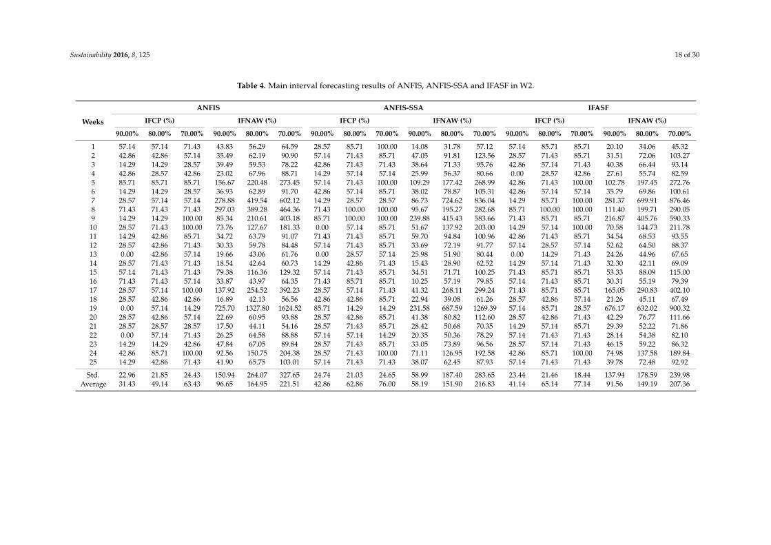
Table 4. Main interval forecasting results of ANFIS, ANFIS-SSA and IFASF in W2.
Weeks
ANFIS ANFIS-SSA IFASF
IFCP (%) IFNAW (%) IFCP (%) IFNAW (%) IFCP (%) IFNAW (%)
90.00% 80.00% 70.00% 90.00% 80.00% 70.00% 90.00% 80.00% 70.00% 90.00% 80.00% 70.00% 90.00% 80.00% 70.00% 90.00% 80.00% 70.00%
1 57.14 57.14 71.43 43.83 56.29 64.59 28.57 85.71 100.00 14.08 31.78 57.12 57.14 85.71 85.71 20.10 34.06 45.322 42.86 42.86 57.14 35.49 62.19 90.90 57.14 71.43 85.71 47.05 91.81 123.56 28.57 71.43 85.71 31.51 72.06 103.273 14.29 14.29 28.57 39.49 59.53 78.22 42.86 71.43 71.43 38.64 71.33 95.76 42.86 57.14 71.43 40.38 66.44 93.144 42.86 28.57 42.86 23.02 67.96 88.71 14.29 57.14 57.14 25.99 56.37 80.66 0.00 28.57 42.86 27.61 55.74 82.595 85.71 85.71 85.71 156.67 220.48 273.45 57.14 71.43 100.00 109.29 177.42 268.99 42.86 71.43 100.00 102.78 197.45 272.766 14.29 14.29 28.57 36.93 62.89 91.70 42.86 57.14 85.71 38.02 78.87 105.31 42.86 57.14 57.14 35.79 69.86 100.617 28.57 57.14 57.14 278.88 419.54 602.12 14.29 28.57 28.57 86.73 724.62 836.04 14.29 85.71 100.00 281.37 699.91 876.468 71.43 71.43 71.43 297.03 389.28 464.36 71.43 100.00 100.00 95.67 195.27 282.68 85.71 100.00 100.00 111.40 199.71 290.059 14.29 14.29 100.00 85.34 210.61 403.18 85.71 100.00 100.00 239.88 415.43 583.66 71.43 85.71 85.71 216.87 405.76 590.3310 28.57 71.43 100.00 73.76 127.67 181.33 0.00 57.14 85.71 51.67 137.92 203.00 14.29 57.14 100.00 70.58 144.73 211.7811 14.29 42.86 85.71 34.72 63.79 91.07 71.43 71.43 85.71 59.70 94.84 100.96 42.86 71.43 85.71 34.54 68.53 93.5512 28.57 42.86 71.43 30.33 59.78 84.48 57.14 71.43 85.71 33.69 72.19 91.77 57.14 28.57 57.14 52.62 64.50 88.3713 0.00 42.86 57.14 19.66 43.06 61.76 0.00 28.57 57.14 25.98 51.90 80.44 0.00 14.29 71.43 24.26 44.96 67.6514 28.57 71.43 71.43 18.54 42.64 60.73 14.29 42.86 71.43 15.43 28.90 62.52 14.29 57.14 71.43 32.30 42.11 69.0915 57.14 71.43 71.43 79.38 116.36 129.32 57.14 71.43 85.71 34.51 71.71 100.25 71.43 85.71 85.71 53.33 88.09 115.0016 71.43 71.43 57.14 33.87 43.97 64.35 71.43 85.71 85.71 10.25 57.19 79.85 57.14 71.43 85.71 30.31 55.19 79.3917 28.57 57.14 100.00 137.92 254.52 392.23 28.57 57.14 71.43 41.32 268.11 299.24 71.43 85.71 85.71 165.05 290.83 402.1018 28.57 42.86 42.86 16.89 42.13 56.56 42.86 42.86 85.71 22.94 39.08 61.26 28.57 42.86 57.14 21.26 45.11 67.4919 0.00 57.14 14.29 725.70 1327.80 1624.52 85.71 14.29 14.29 231.58 687.59 1269.39 57.14 85.71 28.57 676.17 632.02 900.3220 28.57 42.86 57.14 22.69 60.95 93.88 28.57 42.86 85.71 41.38 80.82 112.60 28.57 42.86 71.43 42.29 76.77 111.6621 28.57 28.57 28.57 17.50 44.11 54.16 28.57 71.43 85.71 28.42 50.68 70.35 14.29 57.14 85.71 29.39 52.22 71.8622 0.00 57.14 71.43 26.25 64.58 88.88 57.14 57.14 14.29 20.35 50.36 78.29 57.14 71.43 71.43 28.14 54.38 82.1023 14.29 14.29 42.86 47.84 67.05 89.84 28.57 71.43 85.71 33.05 73.89 96.56 28.57 57.14 71.43 46.15 59.22 86.3224 42.86 85.71 100.00 92.56 150.75 204.38 28.57 71.43 100.00 71.11 126.95 192.58 42.86 85.71 100.00 74.98 137.58 189.8425 14.29 42.86 71.43 41.90 65.75 103.01 57.14 71.43 71.43 38.07 62.45 87.93 57.14 71.43 71.43 39.78 72.48 92.92
Std. 22.96 21.85 24.43 150.94 264.07 327.65 24.74 21.03 24.65 58.99 187.40 283.65 23.44 21.46 18.44 137.94 178.59 239.98Average 31.43 49.14 63.43 96.65 164.95 221.51 42.86 62.86 76.00 58.19 151.90 216.83 41.14 65.14 77.14 91.56 149.19 207.36

Sustainability 2016, 8, 125 19 of 30
In the second part of Experiment III, the interval forecasting results of ARIMA, BPNN, ELM,ARIMA-SSA, BPNN-SSA, ELM-SSA, ANFIS, ANFIS-SSA and IFASF will be demonstrated andcompared (these models have already been briefly introduced in Experiment 2). Table 5 showsthe main interval forecasting results of the nine models by three criteria. IFASF has higher mean IFCPsthan the other models, and only the developed model and ANFIS-SSA meet the 75% standard set inthe CWC criteria, which is a combined index to evaluate the effectiveness of interval forecasts. Similarto the results of Experiment 2, for the CWC criteria, IFASF has the lowest values for 70% and 80%interval forecasts. From the perspective of the interval forecasts’ utility, 90% interval forecasts areinvalid because the highest IFCP of these models is 40%, which is far from the standard 75%. Thus, wewill mainly discuss each models’ effectiveness when forecasting 70% and 80% intervals in this section.For ARIMA and ARIMA-SSA models, the highest IFCP peak is 72.57% using ARIMA pre-processedby SSA for 70% interval forecasts, and the lowest CWC is 664.39, which appears when forecastingthe 80% interval using ARIMA-SSA (this result is the same as the results in Experiment 2). From theboxplot of ARIMA and ARIMA-SSA’s interval forecasts shown in Figure 9b, the SSA method developsthe original ARIMA to obtain better forecasting performance than the original one (CWC is the maincriteria to evaluate the model’s effectiveness).
Table 5. Main interval forecasting results of nine models in W2.
Model
Criteria
Mean IFCP (%) Mean IFNAW (%) Mean CWC (%)
90.00% 80.00% 70.00% 90.00% 80.00% 70.00% 90.00% 80.00% 70.00%
ARIMA 32.57 60.00 72.57 71.00 145.45 180.91 1334.75 701.52 960.76BPNN 30.29 46.29 58.29 72.09 135.75 184.44 915.82 1382.57 2488.25ELM 22.29 45.71 65.71 73.37 130.93 195.32 1886.28 1980.08 1099.05
ANFIS 31.43 49.14 63.43 96.65 164.95 221.51 1948.50 864.88 1849.18ARIMA-SSA 33.14 61.14 72.57 58.21 118.49 172.55 958.31 664.39 811.31BPNN-SSA 32.00 54.86 72.00 60.44 124.56 220.45 1391.35 1031.07 1609.85ELM-SSA 31.43 50.29 72.00 74.16 142.98 208.57 1332.14 2509.92 1045.54
ANFIS-SSA 42.86 62.86 76.00 58.19 151.90 216.83 445.89 1171.13 1721.56IFASF 41.14 65.14 77.14 91.56 149.19 207.36 742.88 327.28 644.70
Comparing BPNN and BPNN-SSA, BPNN-SSA’s CWCs are 1031.07 and 1609.85, which arelower than the 1382.57 and 2488.25 obtained by BPNN when forecasting 70% and 80% wind powerintervals, respectively, indicating that SSA lays a strong foundation to improve the interval forecastingeffectiveness. Notably, the CWC criteria decrease by nearly 30% from the original model to the modelpre-processed by SSA. Figure 9c shows boxplots of the results of BPNN and BPNN-SSA by IFCP,IFNAW and CWC. Similarly, SSA can improve the 70% interval forecasting abilities of BPNN fromthis figure. For the contents in Figure 9f, the forecasting abilities of ELM are also improved usingSSA. Thus, for the benchmark models, SSA can always improve their original models’ forecastingeffectiveness, especially for the 70% interval forecasts. Comparisons among these nine methods will bedemonstrated by two categories: the original models and the models pre-processed by SSA. Table 5shows that ELM only outperforms BPNN when forecasting the 70% interval and that there is not asingle model that outperforms the other models for 70%, 80% and 90% interval forecasts among basicmodels. For models pre-processed by SSA, each model’s forecasting abilities change when utilizingSSA to pre-process the original data. Specifically, ANFIS-SSA is the best method when forecasting 90%intervals and ARIMA-SSA is the best approach for 80% interval forecasts. This result also reflects theresults obtained in Experiment 2 (SSA has a different effect on different models and cannot guaranteethat model M-SSA will outperform model N-SSA if model M outperforms model N).

Sustainability 2016, 8, 125 20 of 30
Sustainability 2016, 8, 125 20 of 31
Figure 9. Boxplots of the IFCPs of models and tables of the improved accuracy percentages of models
by the IFASF model.
However, no matter which model (basic models or models pre‐processed by SSA) is considered,
the IFASF model is still the best interval forecasting model when forecasting 70% and 80% wind
power intervals (see Figure 9a,d,e). In Figure 10, which presents a boxplot of each model when
forecasting 70% and 80% intervals, the blue line represents the mean CWC of 80% interval forecasts,
and the red line represents the mean CWC of 70% interval forecasts. From the perspective of models’
forecasting effectiveness, IFASF apparently outperforms other models no matter which criteria are
Figure 9. Boxplots of the IFCPs of models and tables of the improved accuracy percentages of modelsby the IFASF model.
However, no matter which model (basic models or models pre-processed by SSA) is considered,the IFASF model is still the best interval forecasting model when forecasting 70% and 80% wind powerintervals (see Figure 9a,d,e). In Figure 10, which presents a boxplot of each model when forecasting70% and 80% intervals, the blue line represents the mean CWC of 80% interval forecasts, and the redline represents the mean CWC of 70% interval forecasts. From the perspective of models’ forecastingeffectiveness, IFASF apparently outperforms other models no matter which criteria are considered to

Sustainability 2016, 8, 125 21 of 30
evaluate interval forecasts (such as the median of CWC, the 75th percentile of CWC or the averagevalue of CWC). Thus, from the above analysis of the forecasting results, the developed model, IFASF,is the best interval forecasting model for mean wind power points in the W2 wind farm.
Sustainability 2016, 8, 125 21 of 31
considered to evaluate interval forecasts (such as the median of CWC, the 75th percentile of CWC or
the average value of CWC). Thus, from the above analysis of the forecasting results, the developed
model, IFASF, is the best interval forecasting model for mean wind power points in the W2 wind farm.
Figure 10. Boxplot of each model when forecasting 70% and 80% intervals in W2.
4.2.4. Experiment IV
W3’s interval forecasting effectiveness of ANFIS, ANFIS‐SSA and IFASF, which are evaluated
by IFCP and IFNAW in Table 6, will be first shown in this experiment. From Table 6, the 70% interval
forecast is still more meaningful than other interval forecasts because the IFCP of the 70% forecast is
higher than that of the 80% and 90% interval forecast, indicating that the mean wind power is
unstable data and that it is difficult to forecast its interval to cover its actual values again. Different
from other wind farms, IFCPs of ANFIS, ANFIS‐SSA and IFASF are more than 70% when forecasting
70% mean wind power intervals. Specifically, ANFIS has a 71.43% successful coverage percentage,
ANFIS‐SSA has a 78.29% successful coverage percentage and the IFCP of IFASF peaks at 85.14%.
These results indicate that the SSA and FA play significant roles in improving the coverage
percentage of the mean wind power. From the average values of each column, the IFCPs of IFASF for
the 70%, 80%, and 90% interval forecasts are 44.57%, 66.86% and 85.14%, respectively, which are more
than or equal to the 44.57%, 62.29% and 78.29% obtained by ANFIS‐SSA and the 41.14%, 61.14% and
71.43% obtained by ANFIS. From the perspective of the highest coverage percentage, ANFIS has
five weeks where IFCPs are 100%, the IFCP of ANFIS‐SSA peaks at 100% 13 times, and the developed
model, IFASF, has 18 weeks in which the forecasting interval covers all of the actual mean wind
power points, illustrating that IFASF is a better model to calculate wind power points’ upper bounds
and lower bounds. Specifically, the ANFIS model obtains the highest IFCP when forecasting the 70%
interval in weeks 11, 12, 21 and 25 and forecasting the 80% interval in week 11. The IFCP of the model
developed by SSA peaks at 100% three times when forecasting the 80% interval in weeks 7, 10 and 24
and when forecasting the 70% interval in weeks 2, 7, 9, 12, 17, 19, 24 and 25. For the IFASF model, its
IFCP peaks at 100% 18 times in week 2 for the 70% interval forecast, week 7 for the 70% and 80%
interval forecasts, week 8 for the 70% interval forecast, week 9 for the 70% interval forecast, week 10
for the 70% and 80% interval forecasts, week 11 for the 70% and 80% interval forecasts, week 12 for
the 70% interval, week 17th for 70% interval, week 18 for the 70% interval, week 19 for the 70%, 80%
and 90% intervals, week 24 for the 70% and 80% intervals and week 25 for the 70% interval. For the
purpose of illustrating information in this table, Figure 11 is constructed to show the merits of the
developed model. In Figure 11a, the IFCPs are divided into three categories, which have ranges from
0% to 50%, 50% to 80% and 80% to 100%, and it is obvious that the IFCPs of IFASF or ANFIS‐SSA
belong to (80%~100%) 17 times, which is higher than those of ANFIS, indicating that SSA and FA are
helpful for improving forecasting effectiveness. Figure 11b–d, are histograms of the IFCPs of the three
Figure 10. Boxplot of each model when forecasting 70% and 80% intervals in W2.
4.2.4. Experiment IV
W3’s interval forecasting effectiveness of ANFIS, ANFIS-SSA and IFASF, which are evaluated byIFCP and IFNAW in Table 6, will be first shown in this experiment. From Table 6, the 70% intervalforecast is still more meaningful than other interval forecasts because the IFCP of the 70% forecastis higher than that of the 80% and 90% interval forecast, indicating that the mean wind power isunstable data and that it is difficult to forecast its interval to cover its actual values again. Differentfrom other wind farms, IFCPs of ANFIS, ANFIS-SSA and IFASF are more than 70% when forecasting70% mean wind power intervals. Specifically, ANFIS has a 71.43% successful coverage percentage,ANFIS-SSA has a 78.29% successful coverage percentage and the IFCP of IFASF peaks at 85.14%. Theseresults indicate that the SSA and FA play significant roles in improving the coverage percentage ofthe mean wind power. From the average values of each column, the IFCPs of IFASF for the 70%,80%, and 90% interval forecasts are 44.57%, 66.86% and 85.14%, respectively, which are more than orequal to the 44.57%, 62.29% and 78.29% obtained by ANFIS-SSA and the 41.14%, 61.14% and 71.43%obtained by ANFIS. From the perspective of the highest coverage percentage, ANFIS has five weekswhere IFCPs are 100%, the IFCP of ANFIS-SSA peaks at 100% 13 times, and the developed model,IFASF, has 18 weeks in which the forecasting interval covers all of the actual mean wind power points,illustrating that IFASF is a better model to calculate wind power points’ upper bounds and lowerbounds. Specifically, the ANFIS model obtains the highest IFCP when forecasting the 70% interval inweeks 11, 12, 21 and 25 and forecasting the 80% interval in week 11. The IFCP of the model developedby SSA peaks at 100% three times when forecasting the 80% interval in weeks 7, 10 and 24 and whenforecasting the 70% interval in weeks 2, 7, 9, 12, 17, 19, 24 and 25. For the IFASF model, its IFCPpeaks at 100% 18 times in week 2 for the 70% interval forecast, week 7 for the 70% and 80% intervalforecasts, week 8 for the 70% interval forecast, week 9 for the 70% interval forecast, week 10 for the70% and 80% interval forecasts, week 11 for the 70% and 80% interval forecasts, week 12 for the 70%interval, week 17th for 70% interval, week 18 for the 70% interval, week 19 for the 70%, 80% and 90%intervals, week 24 for the 70% and 80% intervals and week 25 for the 70% interval. For the purposeof illustrating information in this table, Figure 11 is constructed to show the merits of the developedmodel. In Figure 11a, the IFCPs are divided into three categories, which have ranges from 0% to50%, 50% to 80% and 80% to 100%, and it is obvious that the IFCPs of IFASF or ANFIS-SSA belong to

Sustainability 2016, 8, 125 22 of 30
(80%~100%) 17 times, which is higher than those of ANFIS, indicating that SSA and FA are helpful forimproving forecasting effectiveness. Figure 11b–d, are histograms of the IFCPs of the three models,and being more to the right on the IFCP axis indicates a higher IFCP. Thus, the IFASF model’s IFCPsare higher than other models’ IFCPs, demonstrating that SSA and FA actually improve the intervalforecasting ability of ANFIS and show a good pre-processing and optimal effectiveness for randomlyselected weeks. Figure 11e,f illustrate the context of Table 6 and they also show that the proposedmodel is better than ANFIS and ANFIS-SSA for 70%, 80% and 90% interval forecasts.
Sustainability 2016, 8, 125 22 of 31
models, and being more to the right on the IFCP axis indicates a higher IFCP. Thus, the IFASF model’s
IFCPs are higher than other models’ IFCPs, demonstrating that SSA and FA actually improve the
interval forecasting ability of ANFIS and show a good pre‐processing and optimal effectiveness for
randomly selected weeks. Figure 11e,f illustrate the context of Table 6 and they also show that the
proposed model is better than ANFIS and ANFIS‐SSA for 70%, 80% and 90% interval forecasts.
Figure 11. Histograms and plots of the main results of the interval forecasts over 25 weeks in W3.Figure 11. Histograms and plots of the main results of the interval forecasts over 25 weeks in W3.

Sustainability 2016, 8, 125 23 of 30
Table 6. Main interval forecasting results of ANFIS, ANFIS-SSA and IFASF in W3.
Weeks
ANFIS ANFIS-SSA IFASF
IFCP (%) IFNAW (%) IFCP (%) IFNAW (%) IFCP (%) IFNAW (%)
90.00% 80.00% 70.00% 90.00% 80.00% 70.00% 90.00% 80.00% 70.00% 90.00% 80.00% 70.00% 90.00% 80.00% 70.00% 90.00% 80.00% 70.00%
1 42.86 71.43 71.43 28.82 49.93 68.96 42.86 71.43 85.71 25.24 47.04 68.13 42.86 71.43 85.71 27.04 47.81 68.442 42.86 57.14 57.14 43.07 117.98 166.96 57.14 71.43 100.00 84.22 150.44 208.02 42.86 71.43 100.00 70.16 132.64 188.773 42.86 42.86 57.14 24.62 40.36 66.97 28.57 14.29 28.57 8.99 36.07 77.19 28.57 28.57 28.57 35.62 51.67 76.544 28.57 28.57 14.29 26.12 46.82 61.99 28.57 71.43 85.71 5.49 63.09 93.86 14.29 42.86 85.71 28.49 51.97 76.275 57.14 85.71 71.43 71.03 111.75 88.75 42.86 57.14 71.43 33.24 95.48 167.80 71.43 71.43 71.43 62.05 96.46 133.036 42.86 28.57 28.57 224.02 398.30 543.54 71.43 14.29 14.29 515.93 89.52 138.06 42.86 71.43 71.43 73.86 326.57 493.487 71.43 71.43 85.71 268.52 263.36 388.73 71.43 100.00 100.00 144.50 235.77 332.51 57.14 100.00 100.00 125.58 239.55 332.198 57.14 71.43 71.43 112.06 180.12 231.92 28.57 57.14 85.71 76.97 176.41 263.09 42.86 71.43 100.00 117.15 181.48 254.139 28.57 57.14 85.71 44.58 72.33 101.24 42.86 57.14 100.00 47.65 81.81 116.76 42.86 42.86 100.00 42.60 81.00 116.9710 57.14 85.71 85.71 125.02 214.97 302.33 71.43 100.00 100.00 113.43 198.82 277.79 71.43 100.00 100.00 99.18 194.24 276.5311 57.14 100.00 100.00 211.39 369.57 519.13 85.71 85.71 100.00 200.31 356.51 525.20 85.71 100.00 100.00 177.27 362.61 506.8012 28.57 71.43 100.00 66.76 119.23 167.82 0.00 28.57 100.00 49.83 112.32 204.12 0.00 42.86 100.00 72.06 117.04 203.8413 57.14 57.14 85.71 39.77 67.50 94.22 57.14 85.71 85.71 36.41 59.52 92.11 57.14 71.43 85.71 45.92 59.65 95.2614 28.57 42.86 71.43 42.44 76.38 106.24 57.14 71.43 71.43 37.49 74.94 111.06 71.43 85.71 57.14 37.46 75.61 103.4315 14.29 28.57 42.86 10.12 32.07 46.31 0.00 14.29 57.14 19.46 37.67 54.41 0.00 14.29 71.43 16.81 36.65 46.3716 14.29 85.71 71.43 14.93 41.67 60.03 28.57 28.57 42.86 14.40 33.26 48.72 14.29 42.86 71.43 18.63 36.94 56.8717 28.57 57.14 71.43 81.34 101.97 155.20 57.14 71.43 100.00 55.24 93.76 160.18 57.14 71.43 100.00 58.73 103.58 141.1518 42.86 71.43 71.43 70.80 130.53 157.59 42.86 71.43 85.71 59.85 95.46 115.55 42.86 71.43 100.00 52.73 93.67 128.0519 42.86 57.14 57.14 64.84 203.08 310.47 71.43 71.43 100.00 302.35 421.78 587.16 100.00 100.00 100.00 244.05 386.23 533.6320 42.86 71.43 85.71 34.96 47.16 63.78 14.29 71.43 85.71 24.26 41.16 64.07 28.57 85.71 85.71 26.44 47.86 68.3621 28.57 57.14 100.00 12.86 90.24 108.98 42.86 57.14 42.86 21.75 33.45 60.34 28.57 42.86 57.14 23.33 41.60 58.3522 28.57 28.57 42.86 47.19 86.03 120.46 57.14 71.43 28.57 22.84 75.75 113.24 57.14 71.43 71.43 51.11 96.14 130.9523 42.86 57.14 71.43 46.51 69.13 93.71 14.29 42.86 85.71 36.06 72.25 105.74 14.29 28.57 85.71 37.78 57.58 107.1124 42.86 85.71 85.71 89.84 153.37 215.94 42.86 100.00 100.00 90.88 167.52 226.72 42.86 100.00 100.00 90.97 162.37 219.2525 57.14 57.14 100.00 53.84 93.58 129.33 57.14 71.43 100.00 67.09 101.36 134.12 57.14 71.43 100.00 51.15 95.29 124.91
Std. 14.47 20.00 22.21 67.45 97.52 138.17 22.71 25.71 26.76 112.05 98.13 137.47 25.19 24.99 18.66 52.91 102.09 144.13Average 41.14 61.14 71.43 74.22 127.10 174.82 44.57 62.29 78.29 83.76 118.05 173.84 44.57 66.86 85.14 67.45 127.05 181.63

Sustainability 2016, 8, 125 24 of 30
Next, this experiment will show the comparison results among ARIMA, BPNN, ELM,ARIMA-SSA, BPNN-SSA, ELM-SSA, ANFIS, ANFIS-SSA and IFASF in W3. Table 7 shows the maininterval forecasting results of the nine models by three criteria. From this table, IFASF obviously hasa higher mean IFCP than other models and has the lowest CWC among these nine models whenforecasting the wind power interval. From the perspective of the interval forecasts’ utility, 90% intervalforecasts are still invalid because the highest IFCP of these models is 47.43%, which is far from thestandard 75%. Thus, we still mainly discuss each model’s effectiveness when forecasting 70% and80% intervals in this experiment. For the ARIMA and ARIMA-SSA models, the highest IFCP peaks at84% by using ARIMA pre-processed by SSA for 70% interval forecasts, and the lowest CWC is 379.94,which appears when forecasting the 70% interval using ARIMA-SSA.
Table 7. Main interval forecasting results of the nine models in W3.
Model
Criteria
Mean IFCP (%) Mean IFNAW (%) Mean CWC (%)
90.00% 80.00% 70.00% 90.00% 80.00% 70.00% 90.00% 80.00% 70.00%
ARIMA 36.57 62.86 72.57 60.03 125.84 172.12 731.61 782.03 1495.36BPNN 38.29 55.43 66.29 70.45 130.18 147.11 465.93 725.17 1191.36ELM 28.57 57.14 70.86 67.60 124.19 175.83 866.92 725.21 728.27
ANFIS 41.14 61.14 71.43 74.22 127.10 174.82 423.99 497.45 580.47ARIMA-SSA 47.43 69.14 84.00 69.62 126.78 177.31 699.51 482.95 379.94BPNN-SSA 39.43 59.43 77.14 70.80 129.26 180.24 704.34 424.26 324.41ELM-SSA 34.29 62.29 81.71 70.61 127.82 181.16 719.75 366.71 277.05
ANFIS-SSA 44.57 62.29 78.29 83.76 118.05 173.84 431.65 421.26 406.83IFASF 44.57 66.86 85.14 67.45 127.05 181.63 460.78 326.63 269.79
From the perspective of comparisons between BPNN and BPNN-SSA, BPNN-SSA’s CWCs are424.26 and 324.41, which are lower than the 725.17 and 1191.36 obtained by BPNN when forecasting70% and 80% intervals, respectively, indicating that SSA lays a strong foundation to improve theinterval forecasting effectiveness. Notably, the CWC criteria decrease by nearly 57% from the originalmodel to the model pre-progressed by SSA. For other models, SSA can improve their original models’forecasting effectiveness for 70% and 80% interval forecasts. Thus, for the benchmark models, theiroriginal models’ forecasting effectiveness can always be improved, especially for the 70% intervalforecasts. Detailed 70% interval forecast results of each week are listed in Table 8 and the 80% intervalforecast results are in Table 9. Specifically, based on Table 8, the ARIMA model has the highest CWC,18990.21, in the 19th week, and the lowest CWC this model obtains is 90.63, which appears in thefirst week when forecasting the 70% interval. For the 80% interval forecasts which is listed in Table 9,the CWC of ARIMA peaks at 7312.76 in the sixth week and arrives at 65.17 in the 16th. In Table 8, itcan be seen that for the BPNN model, its CWC has the maximum value, 15334.56, in week 11 whenforecasting the 70% mean wind power interval. Alternately, this model provides the best forecastresults in week 16 for the 70% interval forecasts. ELM has the best forecasting performance in week16 when forecasting the 80% interval and has the worst performance in week 6 for the 70% intervalforecasts. In week 16, ANFIS obtains the best forecasting effectiveness for the 70% interval forecasts,and the CWC of this model peaks at 6082.28 in week 6 when forecasting the 70% mean wind powerinterval. For the ARIMA-SSA model, 44.94 is the lowest CWC, obtained in week 20 when forecastingthe 80% interval, and 2687.22 is the highest CWC calculated by this model in week 6 for the 80%interval. BPNN-SSA has the best forecasting performance in week 4 for the 70% interval forecastingand has the worst performance in week 6 for the 80% interval forecasts. In Table 9, The lowest CWCobtained by ELM-SSA is 45.38 when forecasting the 80% interval of the mean wind power in the firstweek. In the contrast, 1265.31 is the highest CWC calculated by this model in the 6th week for the 80%interval forecasts. For the ANFIS-SSA model, its CWC peaks at 3011.94 in week 6 when forecastingthe 70% interval and arrives at 59.52 in week 13 when forecasting the 80% interval. IFASF, the model

Sustainability 2016, 8, 125 25 of 30
developed by SSA and FA, has the best performance in week 20 for the 80% interval forecasts andhas the worst performance in week 6 for the 70% interval forecasts. Regarding the effectiveness ofSSA, it is obvious that each model’s forecasting ability is improved when utilizing SSA to pre-processthe original data: the ARIMA model is improved by 22.90%, 10.00% and 15.75%; the BPNN model isimproved by 3.00%, 7.22% and 16.37%, respectively; the ELM model is improved by 19.57%, 9.01% and15.31%, respectively; and ANFIS is improved by 7.7%, 1.88% and 9.60%, respectively. These resultsindicate that SSA always improves models’ forecasting effectiveness, although SSA has different effectson different models.
Table 8. CWC of each method when forecasting the 70% interval in W3.
WeeksMethods
ARIMA BPNN ELM ANFIS ARIMA-SSA BPNN-SSA ELM-SSA ANFIS-SSA IFASF
1 90.63 209.70 157.66 151.41 108.98 76.60 63.34 68.13 68.442 190.64 169.56 184.16 574.70 203.94 513.50 198.22 208.02 188.773 234.14 2480.27 483.51 230.52 245.94 344.01 486.97 863.73 856.514 274.81 836.33 421.82 1352.39 115.66 74.01 197.16 93.86 76.275 973.54 380.51 390.58 194.85 79.53 232.88 116.30 368.41 292.086 9741.61 4747.14 9690.88 6082.28 1264.97 1197.97 1121.23 3011.94 1083.447 256.68 269.19 279.63 388.73 273.30 312.02 307.72 332.51 332.198 172.96 516.14 730.95 509.18 179.50 225.05 206.94 263.09 254.139 210.76 216.13 211.24 101.24 92.34 109.03 116.12 116.76 116.9710 254.69 633.15 286.85 302.33 261.47 261.24 285.40 277.79 276.5311 504.27 15334.56 1152.26 519.13 423.16 507.54 503.94 525.20 506.8012 157.48 165.68 176.88 167.82 132.58 183.80 387.01 204.12 203.8413 112.30 86.54 95.33 94.22 104.53 197.16 91.34 92.11 95.2614 123.86 298.76 213.59 233.25 123.06 133.23 500.34 243.84 356.0015 117.37 81.57 118.86 277.33 98.49 135.08 211.25 187.30 101.8016 132.38 53.68 61.41 131.80 71.17 247.46 166.31 291.77 124.8617 184.70 149.20 307.81 340.75 189.81 146.35 327.42 160.18 141.1518 148.57 130.90 277.36 345.99 112.57 134.35 130.50 115.55 128.0519 18990.21 618.60 590.81 1068.67 487.85 603.13 776.15 587.16 533.6320 620.36 96.80 133.63 63.78 59.85 158.47 62.84 64.07 68.3621 121.53 163.35 397.71 108.98 148.17 127.08 67.88 361.33 200.8622 3159.35 1653.66 1408.36 721.38 4034.42 1270.82 154.83 1267.22 287.5123 161.75 167.99 89.09 205.74 219.26 301.58 106.71 105.74 107.1124 301.40 203.71 220.01 215.94 318.38 190.71 210.63 226.72 219.2525 147.99 120.79 126.45 129.33 149.52 427.25 129.78 134.12 124.91
Mean 1495.36 1191.36 728.27 580.47 379.94 324.41 277.05 406.83 269.79
Table 9. CWC of each method when forecasting the 80% interval in W3.
WeeksMethods
ARIMA BPNN ELM ANFIS ARIMA-SSA BPNN-SSA ELM-SSA ANFIS-SSA IFASF
1 69.59 100.19 111.81 109.62 180.62 95.49 45.38 103.27 104.972 997.32 511.75 125.22 406.08 162.48 385.94 443.37 330.29 291.213 108.92 677.80 653.63 241.69 276.44 618.79 1177.15 786.93 578.204 168.28 1217.38 570.98 523.87 74.62 495.75 370.74 138.51 311.225 1033.46 456.96 917.12 111.75 179.07 479.68 484.38 328.64 211.776 7312.76 6626.16 6791.56 4457.09 2687.22 2272.72 1265.31 1953.03 716.997 214.60 229.63 202.65 578.21 201.95 225.25 229.35 235.77 239.558 284.89 1003.30 895.77 395.46 125.07 482.17 346.37 607.21 398.449 153.23 380.90 757.76 248.98 154.32 389.81 437.54 281.61 485.0610 736.62 215.79 200.31 214.97 176.52 184.69 204.38 198.82 194.2411 354.86 383.25 1252.93 369.57 302.06 788.67 350.94 356.51 362.6112 113.09 117.27 268.01 261.78 91.03 648.67 470.72 1256.88 700.9213 88.25 185.26 146.29 232.33 83.42 261.87 145.29 59.52 130.9714 210.38 1772.65 413.64 457.38 209.92 374.83 402.55 164.52 75.6115 134.26 717.79 264.59 358.83 97.99 418.43 441.00 821.77 799.4916 65.17 350.80 44.89 41.67 51.62 166.67 144.72 372.22 221.2317 827.65 233.74 226.75 350.98 650.05 189.15 232.91 205.85 227.4218 121.38 498.14 199.93 286.57 198.87 180.46 549.18 209.59 205.6519 1342.65 1035.12 1432.69 699.04 344.05 438.17 418.68 926.02 386.2320 99.49 128.81 97.35 103.53 44.94 112.06 52.82 90.36 47.8621 92.03 129.45 288.26 310.63 114.21 298.78 169.21 115.13 249.1222 2445.81 511.83 1689.43 962.72 2625.09 108.80 161.15 166.32 211.0823 293.01 291.88 139.37 237.95 409.28 404.46 271.39 432.68 644.3724 2158.51 143.50 346.10 153.37 2399.31 292.04 139.99 167.52 162.3725 124.53 209.92 93.20 322.11 233.49 293.10 213.28 222.53 209.22
Mean 782.03 725.17 725.21 497.45 482.95 424.26 366.71 421.26 326.63

Sustainability 2016, 8, 125 26 of 30
Nevertheless, no matter which model (basic models or models pre-progressed by SSA) isconsidered, the IFASF model still is the best interval forecasting model when forecasting the 70% and80% wind power intervals. In Figure 12a, which presents a boxplot of each model when forecasting the70% and 80% intervals, the blue line represents the mean CWC of the 80% interval forecasts, and thered line represents the mean CWC of the 70% interval forecasts. From the perspective of the models’forecasting effectiveness, IFASF apparently outperforms the other models. Thus, from the aboveanalysis of forecasting results, the developed model, IFASF, is the best interval forecasting model forthe mean wind power points in the W3 wind farm.
Sustainability 2016, 8, 125 26 of 31
23 293.01 291.88 139.37 237.95 409.28 404.46 271.39 432.68 644.37
24 2158.51 143.50 346.10 153.37 2399.31 292.04 139.99 167.52 162.37
25 124.53 209.92 93.20 322.11 233.49 293.10 213.28 222.53 209.22
Mean 782.03 725.17 725.21 497.45 482.95 424.26 366.71 421.26 326.63
Nevertheless, no matter which model (basic models or models pre‐progressed by SSA) is
considered, the IFASF model still is the best interval forecasting model when forecasting the 70% and
80% wind power intervals. In Figure 12a, which presents a boxplot of each model when forecasting
the 70% and 80% intervals, the blue line represents the mean CWC of the 80% interval forecasts, and
the red line represents the mean CWC of the 70% interval forecasts. From the perspective of the
models’ forecasting effectiveness, IFASF apparently outperforms the other models. Thus, from the
above analysis of forecasting results, the developed model, IFASF, is the best interval forecasting
model for the mean wind power points in the W3 wind farm.
Figure 12. Boxplot of each model when forecasting the 70% and 80% intervals and illustration of Table 8.
From the results of these four experiments, it is apparent that IFASF is a good model to calculate
the upper and lower bounds for these different wind farms, which means that the developed model
has a good forecasting capability and good adaptability for mean wind power curves of different
wind farms.
4.2.5. Experiment V
In this experiment, we will test the forecasting effectiveness of the proposed model for six‐hour
average wind power in three wind farms (W1, W2 and W3). The CWC results of nine models are
listed in Table 10.
Figure 12. Boxplot of each model when forecasting the 70% and 80% intervals and illustration ofTable 8.
From the results of these four experiments, it is apparent that IFASF is a good model to calculatethe upper and lower bounds for these different wind farms, which means that the developed modelhas a good forecasting capability and good adaptability for mean wind power curves of differentwind farms.
4.2.5. Experiment V
In this experiment, we will test the forecasting effectiveness of the proposed model for six-houraverage wind power in three wind farms (W1, W2 and W3). The CWC results of nine models are listedin Table 10.
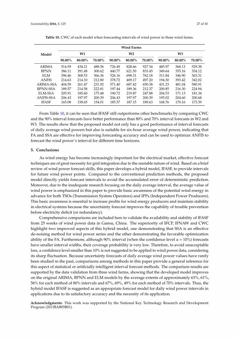
Sustainability 2016, 8, 125 27 of 30
Table 10. CWC of each model when forecasting intervals of wind power in three wind farms.
Model
Wind Farms
W1 W2 W3
90.00% 80.00% 70.00% 90.00% 80.00% 70.00% 90.00% 80.00% 70.00%
ARIMA 514.59 434.21 488.56 726.49 828.66 927.34 485.97 368.13 529.38BPNN 386.11 391.48 300.62 440.77 621.50 833.45 349.64 355.16 354.12ELM 396.46 368.53 366.36 526.16 698.31 762.18 311.84 346.90 363.31
ANFIS 214.63 214.10 212.80 378.72 409.17 497.20 194.30 393.42 342.02ARIMA-SSA 404.59 261.47 231.92 571.40 687.42 650.38 431.23 481.04 580.91BPNN-SSA 189.57 214.58 222.81 197.44 189.36 212.37 200.85 216.30 224.94ELM-SSA 205.91 185.60 175.48 190.72 219.87 247.88 204.53 171.13 181.34
ANFIS-SSA 206.43 197.97 200.39 206.43 197.97 200.39 195.02 204.60 200.68IFASF 165.08 158.65 154.01 185.57 187.15 189.63 168.76 170.16 173.39
From Table 10, it can be seen that IFASF still outperforms other benchmarks by comparing CWCand the 90% interval forecasts have better performance than 80% and 70% interval forecasts in W2 andW3. The results show that the proposed model not only has a good performance of interval forecastsof daily average wind powers but also is suitable for six-hour average wind power, indicating thatFA and SSA are effective for improving forecasting accuracy and can be used to optimize ANFIS toforecast the wind power’s interval for different time horizons.
5. Conclusions
As wind energy has become increasingly important for the electrical market, effective forecasttechniques are of great necessity for grid integration due to the unstable nature of wind. Based on a briefreview of wind power forecast skills, this paper develops a hybrid model, IFASF, to provide intervalsfor future wind power points. Compared to the conventional prediction methods, the proposedmodel directly yields forecast intervals to avoid the accumulated error of deterministic prediction.Moreover, due to the inadequate research focusing on the daily average interval, the average value ofwind power is emphasized in this paper to provide basic awareness of the potential wind energy inadvance for both TSOs (Transmission System Operators) and IPPs (Independent Power Producers).This basic awareness is essential to increase profits for wind energy producers and maintain stabilityin electrical systems because the uncertainty forecast improves the capability of trouble preventionbefore electricity deficit (or redundancy).
Comprehensive comparisons are included here to validate the availability and stability of IFASFfrom 25 weeks of wind power data in Gansu, China. The superiority of IFCP, IFNAW and CWChighlight two improved aspects of this hybrid model, one demonstrating that SSA is an effectivede-noising method for wind power series and the other demonstrating the favorable optimizationability of the FA. Furthermore, although 90% interval (when the confidence level α = 10%) forecastshave smaller interval widths, their coverage probability is very low. Therefore, to avoid unacceptableloss, a confidence level smaller than 10% is not suggested to be applied to wind power data, consideringits sharp fluctuation. Because uncertainty forecasts of daily average wind power values have rarelybeen studied in the past, comparisons among methods in this paper provide a general reference forthis aspect of statistical or artificially intelligent interval forecast methods. The comparison results aresupported by the data validation from three wind farms, showing that the developed model improveson the original ARIMA, BPNN and ELM models by the average extents of approximately 63%, 61%,56% for each method of 80% intervals and 67%, 69%, 49% for each method of 70% intervals. Thus, thehybrid model IFASF is suggested as an appropriate forecast model for daily wind power intervals inapplications due to its satisfactory accuracy and the necessity of its application.
Acknowledgments: This work was supported by the National Key Technology Research and DevelopmentProgram (2013BAB05B01).
Sustainability 2016, 8, 125 28 of 30
Author Contributions: Zhongrong Zhang and Feng Liu designed experiments; Feng Liu and Yiliao Song carriedout experiments; Feng Liu analyzed experimental results. Zhongrong Zhang analyzed sequencing data anddeveloped analysis tools. Jinpeng Liu assisted with Illumina sequencing. Zhongrong Zhang, Yiliao Song andFeng Liu wrote the manuscript.
Conflicts of Interest: The authors declare no conflict of interest.
Acronyms
FA Firefly AlgorithmSSA Singular Spectrum AnalysisPCA Principal Component AnalysisNWP Numeric Weather PredictionFIS Fuzzy Inference SystemELM Extreme Learning MachineANFIS Adaptive-Network-Based Fuzzy Inference SystemIFNAW Interval Forecast Normalized Average WidthIFCP Interval Forecast Coverage ProbabilityCWC Coverage Width-based CriteriaBPNN Back Propagation Neural NetworkARIMA Autoregressive Integrated Moving Average Model
Appendix
IFCP shows the coverage probability of target values between lower and upper limits with thefollowing form [44]:
IFCP pyi, Ui, Liq “1n
nÿ
i“1
ILiďyiďUi pyiq (A1)
where yi is the real value, n denotes the sample size. Ui and Li are separately the upper and lowerprediction of yi. ILiďyiďUi pyiq is the indicative function, equaling 1 if Li ď yi ď Ui and 0 if not.
IFNAW quantifies the normalized average width of the interval and is computed by the followingformula [45]:
IFNAW “1
nR
nÿ
i“1
pUi ´ Liq (A2)
where R is the difference between the maximum and minimum values.Based on the above two criteria, the coverage width-based criterion is proposed to summarize
the interval forecasting ability including coverage probability and interval width. It is computed asfollows [44,45]:
CWC “ IFNAW ˆ
1` IIFCPăµ pIFCPq exp p´η pIFCP´ µqq(
(A3)
where µ is determined by the nominal confidence level, while η is usually a large value to magnifythe difference between IFCP and µ. IIFCPăµ pIFCPq denotes the indicator function and equals 1 ifIFCP ă µ.
References
1. Ramirez-Rosado, I.J.; Fernandez-Jimenez, L.A.; Monteiro, C.; Sousa, J.; Bessa, R. Comparison of two newshort-term wind-power forecasting systems. Renew. Energy 2009, 34, 1848–1854. [CrossRef]
2. National Energy Administration 2014. Available online: http://www.nea.gov.cn/2015-02/12/c_133989991.htm(accessed on 25 January 2016).
3. National Energy Administration 2015. Available online: http://www.nea.gov.cn/2015-06/08/c_134305870.htm(accessed on 25 January 2016).

Sustainability 2016, 8, 125 29 of 30
4. Sideratos, G.; Hatziargyriou, N.D. Wind Power Forecasting Focused on Extreme Power System Events.IEEE Trans. Sustain. Energy 2012, 3, 445–454. [CrossRef]
5. Zhao, P.; Wang, J.; Xia, J.; Dai, Y.; Sheng, Y.; Yue, J. Performance evaluation and accuracy enhancement of aday-ahead wind power forecasting system in China. Renew. Energy 2012, 43, 234–241. [CrossRef]
6. Bhaskar, K.; Singh, S.N. AWNN-Assisted Wind Power Forecasting Using Feed-Forward Neural Network.IEEE Trans. Sustain. Energy 2012, 3, 306–315. [CrossRef]
7. Han, L.; Romero, C.E.; Yao, Z. Wind power forecasting based on principle component phase spacereconstruction. Renew. Energy 2015, 81, 737–744. [CrossRef]
8. Traiteur, J.J.; Callicutt, D.J.; Smith, M.; Roy, S.B. A short-term ensemble wind speed forecasting system forwind power applications. J. Appl. Meteorol. Climatol. 2012, 51, 1763–1774. [CrossRef]
9. Silva, L. A feature engineering approach to wind power forecasting. Int. J. Forecast. 2014, 30, 395–401.[CrossRef]
10. Mahoney, W.P.; Parks, K.; Wiener, G.; Liu, Y.; Myers, W.L.; Sun, J.; Delle Monache, L.; Hopson, T.; Johnson, D.;Haupt, S.E. A Wind Power Forecasting System to Optimize Grid Integration. IEEE Trans. Sustain. Energy2012, 3, 670–682. [CrossRef]
11. Croonenbroeck, C.; Dahl, C.M. Accurate medium-term wind power forecasting in a censored classificationframework. Energy 2014, 73, 221–232. [CrossRef]
12. Karayiannis, N.B.; Member, S.; Randolph-gips, M.M. Probabilistic Wind Power Forecasting Using RadialBasis Function Neural Networks. Power Syst. IEEE Trans. 2003, 14, 835–846.
13. Kou, P.; Gao, F.; Guan, X. Sparse online warped Gaussian process for wind power probabilistic forecasting.Appl. Energy 2013, 108, 410–428. [CrossRef]
14. Bessa, R.J.; Miranda, V.; Botterud, A.; Wang, J. Time Adaptive Conditional Kernel Density Estimation forWind Power Forecasting. IEEE Trans. Sustain. Energy 2012, 3, 660–669. [CrossRef]
15. Carpinone, A.; Giorgio, M.; Langella, R.; Testa, A. Markov chain modeling for very-short-term wind powerforecasting. Electr. Power Syst. Res. 2015, 122, 152–158. [CrossRef]
16. Pinson, P. Very-short-term probabilistic forecasting of wind power with generalized logit—Normaldistributions. J. R. Stat. Soc. Ser.C Appl. Stat. 2012, 555–576. [CrossRef]
17. Bessa, R.J.; Miranda, V.; Botterud, A.; Zhou, Z.; Wang, J. Time-adaptive quantile-copula for wind powerprobabilistic forecasting. Renew. Energy 2012, 40, 29–39. [CrossRef]
18. Pinson, P.; Nielsen, H.A.; Madsen, H.; Kariniotakis, G. Skill forecasting from ensemble predictions of windpower. Appl. Energy 2009, 86, 1326–1334. [CrossRef]
19. Pinson, P.; Madsen, H.; Papaefthymiou, G. From Probabilistic Forecasts to Wind Power Production. Production2009, 12, 51–62.
20. Qin, S.; Liu, F.; Wang, J.; Song, Y. Interval forecasts of a novelty hybrid model for wind speeds. Energy Rep.2015, 1, 8–16. [CrossRef]
21. Jursa, R.; Rohrig, K. Short-term wind power forecasting using evolutionary algorithms for the automatedspecification of artificial intelligence models. Int. J. Forecast. 2008, 24, 694–709. [CrossRef]
22. Monteiro, C.; Bessa, R.; Miranda, V.; Botterud, A.; Wang, J.; Conzelmann, G. Wind Power Forecasting:State-of-the-Art 2009 Decision and Information Sciences Division; Argonne National Laboratory: Lemont,IL, USA, 2009; pp. 1–216.
23. Foley, A.M.; Leahy, P.G.; Marvuglia, A.; McKeogh, E.J. Current methods and advances in forecasting of windpower generation. Renew. Energy 2012, 37, 1–8. [CrossRef]
24. Sideratos, G.; Hatziargyriou, N.D. An Advanced Statistical Method for Wind Power Forecasting. IEEE Trans.Power Syst. 2007, 22, 258–265. [CrossRef]
25. Shi, J.; Ding, Z.; Member, S.; Lee, W.; Yang, Y.; Liu, Y.; Analysis, A.G.R. Hybrid forecasting model forvery-short term wind power forecasting based on grey relational analysis and wind speed distributionfeatures. IEEE Trans. Smart Grid 2014, 5, 521–526. [CrossRef]
26. Croonenbroeck, C.; Stadtmann, G. Minimizing asymmetric loss in medium-term wind power forecasting.Renew. Energy 2015, 81, 197–208. [CrossRef]
27. Broomhead, D.S.; King, G.P. Extracting qualitative dynamics from experimental data. Phys. DNonlinear Phenom. 1986, 20, 217–236. [CrossRef]
28. Jang, J.R. ANFIS: Adaptive-Network-Based Fuzzy Inference System. IEEE Trans. Syst. Man Cybern. 1993, 23,665–685. [CrossRef]
Sustainability 2016, 8, 125 30 of 30
29. Yang, X. Firefly algorithms for multimodal optimization, in Stochastic Algorithms: Foundations andApplications (SAGA 2009). Stoch. Algorithms Found. Appl. 2009, 5792, 169–178.
30. Vautard, R.; Yiou, P.; Ghil, M. Singular-spectrum analysis A toolkit for short, noisy chaotic signals. Phys. DNonlinear Phenom. 1992, 58, 95–126. [CrossRef]
31. Kondrashov, D.; Shprits, Y.; Ghil, M. Gap filling of solar wind data by singular spectrum analysis.Geophys. Res. Lett. 2010, 37, 1–6. [CrossRef]
32. Hsieh, W.W.; Hamilton, K. Nonlinear singular spectrum analysis of the tropical stratospheric wind. Q. J. R.Meteorol. Soc. 2003, 129, 2367–2382. [CrossRef]
33. Takens, F. Detecting strange attractors in turbulence. Dyn. Syst. Turbul. Warwick 1980 1981, 898, 366–381.34. Liu, Y.-F.; Zhao, M. De-Noising of Chaotic Time Series Based on Singular Spectrum Analysis. J. Shanghai
Jiaotong Univ. 2003, 37, 778–780.35. Mohandes, M.; Rehman, S.; Rahman, S.M. Estimation of wind speed profile using adaptive neuro-fuzzy
inference system (ANFIS). Appl. Energy 2011, 88, 4024–4032. [CrossRef]36. Pousinho, H.M.I.; Mendes, V.M.F.; Catalão, J.P.S. A hybrid pso-anfis approach for short-term wind power
prediction in Portugal. Energy Convers. Manag. 2011, 52, 397–402. [CrossRef]37. Takagi, T.; Sugeno, M. Fuzzy identification of systems and its applications to modeling and control.
IEEE Trans. Syst. Man Cybern. 1985, SMC-15, 116–132. [CrossRef]38. Hiremath, S.M.; Patra, S.K.; Mishra, A.K. Extended date rate prediction for cognitive radio using ANFIS
with Subtractive Clustering. In Proceedings of the 2012 5th International Conference on Computers andDevices for Communication (CODEC), Kolkata, Calcutta, 17–19 December 2012.
39. Chiu, S.L. Fuzzy Model Identification Based on Cluster Estimation. J. Intell. Fuzzy Syst. 1994, 2, 267–278.40. Chen, M.Y. A hybrid ANFIS model for business failure prediction utilizing particle swarm optimization and
subtractive clustering. Inf. Sci. 2013, 220, 180–195. [CrossRef]41. Yu, J.; Chen, K.; Mori, J.; Rashid, M.M. A Gaussian mixture copula model based localized Gaussian process
regression approach for long-term wind speed prediction. Energy 2013, 61, 673–686. [CrossRef]42. Wan, C.; Xu, Z.; Pinson, P. Direct interval forecasting of wind power. IEEE Trans. Power Syst. 2013, 28,
4877–4878. [CrossRef]43. Geng, J.; Huang, M.; Li, M.; Hong, W. Neurocomputing Hybridization of seasonal chaotic cloud simulated
annealing algorithm in a SVR-based load forecasting model. Neurocomputing 2015, 151, 1362–1373. [CrossRef]44. Quan, H.; Srinivasan, D.; Khosravi, A. Short-term load and wind power forecasting using neural
network-based prediction intervals. IEEE Trans. Neural Netw. Learn. Syst. 2014, 25, 303–315. [CrossRef][PubMed]
45. Khosravi, A.; Nahavandi, S.; Creighton, D. Prediction intervals for short-term wind farm power generationforecasts. IEEE Trans. Sustain. Energy 2013, 4, 602–610. [CrossRef]
© 2016 by the authors; licensee MDPI, Basel, Switzerland. This article is an open accessarticle distributed under the terms and conditions of the Creative Commons by Attribution(CC-BY) license (http://creativecommons.org/licenses/by/4.0/).


![Sample Exercise 14.1 Calculating an Average Rate of … average rate of reaction over this time interval. Plan: The average rate is given by the change in concentration, Δ[A], divided](https://img.pdfslide.us/doc/110x75/5afeed9a7f8b9a994d8facbb/sample-exercise-141-calculating-an-average-rate-of-average-rate-of-reaction.jpg)