Embed Size (px)
Citation preview

WINNER II D2.2.3 v1.0
Page 1 (117)
IST-4-027756 WINNER II D2.2.3 Modulation and Coding schemes for the WINNER II System
Contractual Date of Delivery to the CEC: 2007-11-30
Actual Date of Delivery to the CEC: 2007-11-29
Author(s): Thierry Lestable, Yi Ma, Monica Navarro, Adam Piątyszek, Stephan Pfletschinger (editor), Christian Senger, Mikael Sternad, Tommy Svensson
Participant(s): CTH, CTTC, NSN, PUT, SEUK, UniS
Workpackage: WP2 Link
Estimated person months: 30 PM
Security: PU
Nature: R
Version: 1.0
Total number of pages: 117
Abstract:
This report describes the modulation and coding schemes for the WINNER II system, considering detailed aspects of channel coding. Two modes for link adaptation are illustrated and a scheme for H-ARQ is defined.
Keyword list:
LDPC, DBTC, link adaptation, adaptive coding and modulation (ACM), bit-loading, H-ARQ, incremental redundancy
Disclaimer:

WINNER II D2.2.3 v1.0
Page 2 (117)
Executive Summary The main focus of this document is to capture leading-edge technologies related with Channel Coding, Link Adaptation and H-ARQ investigated during this 2nd phase of WINNER, whilst maintaining consistency with directions and conclusions from WINNER Phase I.
Refinements and optimizations of Advanced Channel Coding candidates from Phase-I, respectively Duo-Binary Turbo-Codes (DBTC) and Quasi-Cyclic Block-Low-Density Parity-Check (QC-BLDPC) Codes have been focusing on enabling key features such as Rate-Compatibility through Puncturing (RCP) for making full usage of advantages of Incremental Redundancy (IR) Hybrid-ARQ scheme (Type-II), together with targeting higher codeword lengths (Lifting of LDPC codes).
Besides, thanks to tight discussions with Concept Groups introduced in Phase II, particular attention has been paid to coding of control signalling information (short packets), especially focusing on the Broadcast Channel (BCH) robustness which directly impacts the coverage capabilities of the system. For this purpose an existing solution based on Optimum Distance Spectrum (ODS) Convolutional Codes is highlighted, and finally promoted as a suitable, and promising candidate thanks to fair evaluation, and comparison w.r.t. Phase-I proposal.
Furthermore, a brand new Link Adaptation algorithm based on Mutual-Information approach, has been proposed, designed, and tuned w.r.t. the advanced channel coding candidates. In-depth evaluations, and comparisons, taking into account multiple impairments (e.g. prediction errors) outline the outstanding performance enhancement brought by such new and innovative approach.
Finally, an innovative framework of H-ARQ is introduced for the first time, leading to flexible and efficient handling of joint Link Adaptation, Incremental Redundancy and Repetition coding. This enables the thorough evaluation of the achievable throughput and delay whilst combining Link Adaptation with H-ARQ.
Through the whole document, multiple valuable complementary evaluations have been performed to refine the pros and cons of the above mentioned solutions, ensuring a sufficient wide range of performance results strengthening the final solutions promoted in this document whilst targeting Next Generation Wireless Cellular systems.

WINNER II D2.2.3 v1.0
Page 3 (117)
Authors Partner Name Phone / Fax / e-mail
CTH/UU Mikael Sternad Phone: +46 704 250 354 Fax: +46 18 555 096 e-mail: [email protected] Tommy Svensson Phone: +46 31 772 1823 Fax: +46 31 772 1782 email: [email protected]
CTTC Monica Navarro Phone: +34 93 645 2915 Stephan Pfletschinger Fax: +34 93 645 2901 e-mail: [email protected] [email protected]
NSN/UU Christian Senger Phone: +49 731 50 315 36 Fax: +49 731 50 315 09 e-mail: [email protected]
PUT Adam Piątyszek Phone: +48 61 665 3936 Fax: +48 61 665 3823 e-mail: [email protected]
SEUK Thierry Lestable Phone: +44 1784 428600 (Ext.720) Fax: +44 1784 428624 e-mail: [email protected]
UniS Yi Ma Phone: +44 1483 683427 Fax: +44 1483 686011 e-mail: [email protected]

WINNER II D2.2.3 v1.0
Page 4 (117)
Table of Contents
1. Introduction ................................................................................................. 7
2. Modulation and Coding ............................................................................ 11 2.1 Modulation and Coding Schemes with Duo-Binary Turbo Codes ............................................ 11
2.1.1 Detailed Description of DBTC.......................................................................................... 11 2.1.2 DBTC Performance Results .............................................................................................. 15 2.1.3 Analytical Approximation of CWER Curves.................................................................... 16
2.2 Quasi-Cyclic Block LDPC Codes ............................................................................................. 18 2.2.1 Encoding of BLDPC Codes .............................................................................................. 20 2.2.2 Decoding of BLDPC Codes .............................................................................................. 22 2.2.3 Rate-Compatible Puncturing of BLDPC Codes ................................................................ 22 2.2.4 Performance Results for RCP BLDPC Codes................................................................... 22 2.2.5 Low Coding Rate BLDPC Code ....................................................................................... 23 2.2.6 Lifting process for QC-BLDPC Codes ............................................................................. 24 2.2.7 SNR Mismatch Impact on LDPC Codes........................................................................... 25
2.3 Low rate convolutional codes for broadcast information .......................................................... 28 2.4 Choice of Coding Scheme for Reference Design ...................................................................... 30 2.5 Conclusions ............................................................................................................................... 32
3. Link Adaptation......................................................................................... 33 3.1 Introduction ............................................................................................................................... 33 3.2 Basic Considerations for Link Adaptation................................................................................. 34
3.2.1 Mutual information based averaging of SNR values ........................................................ 34 3.2.2 Channel Prediction Error Model for Frequency-Adaptive Transmission.......................... 34 3.2.3 The Impact of Prediction Errors........................................................................................ 35 3.2.4 Review of channel prediction performance....................................................................... 39
3.3 Frequency-Adaptive Transmission............................................................................................ 43 3.3.1 The MI-ACM Bit-Loading Algorithm .............................................................................. 43 3.3.2 Application of DBTC to the MI-ACM Algorithm ............................................................ 45 3.3.3 Fine Tuning of MI-ACM Algorithm with RCP BLDPC Codes........................................ 46 3.3.4 Performance of ACM for Multiple-Users ......................................................................... 52
3.4 Non-Frequency Adaptive Transmission .................................................................................... 53 3.5 Conclusions ............................................................................................................................... 54
4. Hybrid Automatic Repeat Request (HARQ) ............................................ 56 4.1 Introduction ............................................................................................................................... 56
4.1.1 The MAC Concept ............................................................................................................ 56 4.1.2 Hop-by-Hop ARQ Technology Options ........................................................................... 57 4.1.3 Flexible Hybrid-ARQ Type II Scheme Based on Soft Bit Interface ................................. 58

WINNER II D2.2.3 v1.0
Page 5 (117)
4.2 Incremental Redundancy Scheme.............................................................................................. 59 4.2.1 Simulation Results ............................................................................................................ 60
4.3 Throughput and Delay Analysis for Partial CQI ....................................................................... 63 4.4 Error Detection Capabilities of LDPC Codes............................................................................ 66 4.5 Allocation Schemes ................................................................................................................... 68
4.5.1 Simulation Results for Frequency-Adaptive Transmission Mode .................................... 70 4.5.2 Simulation Results for Non Frequency-Adaptive Transmission Mode............................. 70
4.6 Conclusions ............................................................................................................................... 73
5. Concluding Remarks and Outlook .......................................................... 74
Appendix A. Modulation and Coding ...................................................... 75 A.1 DBTC Details and Performance Results ................................................................................... 75 A.2 RCP BLDPC Performance Results............................................................................................ 78 A.3 Base Matrix for R = ½ RCP BLDPC Code ............................................................................... 82 A.4 Base-Model Matrix and A-list format for Low Code Rate (1/3) LDPC Code........................... 83 A.5 Performance Results for Low-Code Rate (1/3) BLDPC Code .................................................. 85 A.6 Lifted base-matrices for QC-BLDPC Codes ............................................................................. 88 A.7 SNR Mismatch Impact on LDPC Codes ................................................................................... 92
Appendix B. Link Adaptation................................................................... 97 B.1 Impact of Channel Estimation and Prediction Error.................................................................. 97 B.2 Impact of using R = 1.0 code rate in MI-ACM algorithm with RCP BLDPC codes............... 102
Appendix C. Link Adaptation for Cooperative Relaying (Yi Ma)......... 103 C.1 System Model and Objective................................................................................................... 103 C.2 BPL Criterion for the Ideal SLS-DF Relay ............................................................................. 104 C.3 BPL Criterion for the Outage SLS-DF Relay.......................................................................... 106 C.4 Simulation Results................................................................................................................... 107
References.................................................................................................... 115

WINNER II D2.2.3 v1.0
Page 6 (117)
List of Acronyms and Abbreviations
ARQ Automatic Repeat Request AWGN Additive White Gaussian Noise B-EFDMA Block-Equidistant Frequency Division Multiple Access B-IFDMA Block-Interleaved Frequency Division Multiple Access BER Bit Error Rate BLDPCC Block LDPC Code BP Belief Propagation BPL Bit and Power Loading BPSK Binary Phase Shift Keying BS Base Station CC Convolutional Code CDF Cumulative Density Function CQI Channel Quality Information CRC Cyclic Redundancy Check CWER Code Word Error Rate DBTC Duo-Binary Turbo Code FDD Frequency Division Duplex FEC Forward Error Correction (Coding) GMC Generalised Multi-Carrier GoB Grid of Beams HARQ Hybrid Automatic Repeat Request IFDMA Interleaved Frequency Division Multiple Access IR Incremental Redundancy IT Initial Transmission LDPC Low-Density Parity-Check Code LLR Log-Likelihood Ratio LoS Line-of-Sight MAC Medium Access Control MCS Modulation and Coding Scheme MI Mutual Information (link-to-system level interface, [BAS+05]) MI-ACM Mutual Information based Adaptive Coding and Modulation MIMO Multiple Input Multiple Output MMSE Minimum Mean Square Error MSE Mean Square Error ODS Optimum Distance Spectrum OFDM Orthogonal Frequency Division Multiplexing OFDMA Orthogonal Frequency Division Multiple Access PDF Probability Density Function PHY Physical (layer) QAM Quadrature Amplitude Modulation QC-BLDPCC Quasi-Cyclic Block LDPC Code QoS Quality of Service QPSK Quadrature Phase Shift Keying RAN Radio Access Network RCP Rate Compatible Punctured RN Relay Node. RT ReTransmission RTU ReTransmission Unit SINR Signal to Interference and Noise Ratio SISO Single-Input Single-Output SNR Signal to Noise Ratio TDD Time Division Duplex TDMA Time Division Multiple Access UT User Terminal

WINNER II D2.2.3 v1.0
Page 7 (117)
1. Introduction The present report describes modulation and coding schemes for the WINNER II system. Its main contributions are
• improved coding schemes, with detailed descriptions of implementations,
• a novel adaptive transmission technique with superior performance,
• a flexible retransmission (Hybrid ARQ) scheme, and
• link level performance evaluation result for all these proposed schemes.
These schemes are parts of the over-all WINNER reference design described in [WIN2D61314].
The results are based on previous work performed within the WINNER project in 2004-2005, here called WINNER phase 1. Let us summarize these previous results to place the present results in context.
Generalized Multicarrier transmission (GMC) has been used within the WINNER project. GMC configured as standard cyclic-prefixed (CP) OFDM was selected in WINNER phase 1 for the downlinks and uplinks where terminal power consumption is not a limiting factor. GMC configured as serial modulation (DFT precoded CP-OFDM) was recommended for power-limited uplinks, since this transmission technology is power efficient [WIN1D210]. At the end of WINNER phase 1, several possible types of DFT-precoding were under consideration. As modulation schemes, BPSK and square M-QAM were considered, using M = 4, 16 and 64.
WINNER phase 1 introduced two basic types of adaptive transmission (cf. Section 3.1.6 of [WIN1D210]):
• Frequency-adaptive transmission, where payload bits from flows are allocated to rectangular time-frequency-spatial resource units that are denoted chunk layers. The allocation scheme is thus denoted as chunk-based TDMA/OFDMA. Individual link adaptation may be performed within each chunk layer. This link adaptation is adjusted to the frequency selective small-scale fading.
• Non-frequency adaptive transmission averages over the frequency-selective fading. A code block is here interleaved and mapped onto a dispersed set of time-frequency-spatial transmission resources. The same link adaptation parameters (modulation and code rate) are used for the whole code block.
The preliminary WINNER II baseline design for these adaptive transmission types were outlined in [WIN2D6137]. The updated final reference designs are presented in [WIN2D61314].
The investigations of WINNER phase 1, described in [WIN1D23] and [WIN1D210], led to a recommendation that convolutional codes should be used for the smallest code block sizes, below 200 bits. Duo-binary turbo codes were recommended for intermediate block sizes, while quasi-cyclic block LDPC codes gave the best performance for the largest block lengths (cf. Figure B.5 in Annex B.2 of [WIN1D210]). The work in WINNER II has built on these results, with the purpose of improving the coding schemes where required, and down-selecting the number of recommended coding schemes for the final system concept.
The best way of implementing frequency-adaptive transmission of Winner phase 1 was to use individually adjusted code and modulation rates within each chunk layer, see [WIN1D24]. Since the number of symbols per chunk is rather small, convolutional coding is appropriate and was used in these investigations. This method works well, but the small block size limits the attainable coding gain. In WINNER II, we have investigated how the performance can be improved by combining chunk-individual link adaptation with coding over larger code blocks, using stronger codes like LDPC or Turbo codes.
Retransmission schemes were not investigated in WINNER phase 1. WINNER II investigations have developed a link retransmission scheme that is based on the recommended coding methods.
The new results on modulation, coding, link adaptation and retransmission will be presented in three main chapters:
Chapter 2, on modulation and coding • A description and performance results for duo-binary turbo codes (DBTC) can be found in
Section 2.1. An additional useful result in Section 2.1.3 is that it is possible to very well

WINNER II D2.2.3 v1.0
Page 8 (117)
approximate the codeword error rate curves by exponential functions. These approximations are then used in further analytical and semi-analytical investigations in Chapters 3 and 4.
• A detailed description of encoding, decoding and puncturing of quasi-cyclic block LDPC codes is given in Section 2.2. The WINNER baseline design described in [WIN2D6137] uses rate-compatible codes with base rate ½, with performance results for two block lengths, 288 and 1152 bits. In the final system concept, the base code rate has been changed to rate 1/3, to improve the performance of retransmission schemes. Code word error rate results for these codes are presented Appendix A.5 The LDPC results have furthermore been extended to much larger block sizes by a lifting process, see Section 2.2.6. This enables very high data rates without requiring an excessive number of stop-and-wait retransmission channels. The sensitivity of the decoding results to SNR errors (mismatch) at the receiver is finally investigated in Section 2.2.7.
• Convolutional codes that use tail-biting are needed in small code blocks, in particular for control signalling. Such codes have been investigated in Section 2.3 for code block sizes down to 25 bits and mother code rate ¼. They have contributed to reducing the control overhead.
• Within the considered range of packet lengths, LDPC codes and duo-binary turbo codes provide similar performance. Since the WINNER concept should contain a minimal number of alternatives that provide similar performance, one of these schemes was selected for the final WINNER concept. As motivated in Section 2.4, the choice is the quasi-cyclic block-LDPC scheme.
All performance results for DBTC and LDPC codes over AWGN channels will be published on the WINNER web page.
Chapter 3, on link adaptation • When mapping a codeword onto a set of transmission resources with differing SINR, a tool is
needed for predicting/estimating the resulting code word error rate from the set of SINRs. Such a tool can be used for several purposes:
o As link-to-system interfaces in system level simulators, which use these predicted codeword error rates and do not need to implement the complete decoding.
o As a component of the link adaptation scheme described below, where a codeword is mapped onto a set of chunk layers, with varying individual link adaptations and SINRs.
Within WINNER, a mutual information based averaging of SINR values has been developed and has been found to provide the best performance among many investigated alternatives [BAS+05]. It is outlined in Section 3.2.1.
• The WINNER reference algorithms for frequency adaptive transmission is outlined in Section 3.3. It is denoted as MI-ACM (mutual information based adaptive coding and modulation) scheme, also known as Stiglmayr’s algorithm. It has been used for the WINNER II baseline design [WIND6137] and is included unaltered in the final WINNER reference design. Briefly, link adaptation is used that applies constant transmit power but adjusts the modulation per chunk layer. An average puncturing and code rate for the whole code block is calculated for the so link-adapted resources. The punctured block is interleaved and mapped onto the chunk layers. In this way, strong codes that work best with large code blocks can be combined with fine-grained link adaptation of resources within code blocks. The resulting scheme has been shown to work better than using individual code blocks per chunk layer. It can be used in combination with LDPC codes as well as Turbo codes (Section 3.3.2).
• Adjustment SINR of limits for using different modulation and code rates and the appropriate combinations of modulation and code rates are investigated in Section 3.3.3. The MI-ACM algorithm is used here together with rate compatible duo-binary Turbo codes. The modulation rates are extended to 256-QAM. The use of 8-QAM, 32-QAM and 128-QAM is investigated, but is found to be of no use in combination with the investigated code rates.
Chapter 4, on Hybrid ARQ • A flexible Hybrid ARQ (incremental redundancy) retransmission scheme is proposed and
investigated in Section 4.2. Briefly, the scheme starts with a codeword encoded at the mother code rate (1/3). Assume that the first N3 bits are systematic bits (the uncoded segment).

WINNER II D2.2.3 v1.0
Page 9 (117)
o The first transmission then uses the first N2 bits, where N3/N2 is the appropriate code rate.
o If there are unused resources in the allocated chunk layers, a separate investigation in Section 4.5 concludes that it is best to fill these by extending initial transmissions with additional parity bits.
o If a retransmission is then required, additional parity bits are transmitted, using a link adaptation that is appropriate for that transmission. Soft bit combining is used at the receiver.
o When reaching the end of the codeword, the retransmissions starts anew from the beginning of the codeword.
This scheme provides a seamless transition from incremental redundancy to chase combining for many retransmissions. The retransmission block size is adjustable. This scheme works with a 1-bit ACK feedback. It is integrated without problem into the n-channel stop and wait link retransmission protocol of the WINNER reference design.
• The initial transmission and its link adaptation would be based on predicted channel quality information i.e. separate SINR values of all chunks for frequency adaptive transmission, and an average SINR for non-frequency adaptive transmission. The retransmission mechanism then acts as a safety net. The need for retransmissions is affected by the statistics of the prediction error. It is also affected by the criterion used for adjusting the modulation and code rate limits. The impact of prediction errors has been investigated extensively in Sections 2.2.2 and 3.1 of [WIND24], where the modulation and coding rate limits are adjusted to attain a target packet error rate also in the presence of prediction errors [FSE+04]. The packet error rate should then remain constant, so the number of retransmissions is not affected by the prediction error variance. If the modulation rate limits are instead adjusted to maximize the throughput [SF04], a larger initial prediction error will result in more frequent retransmissions. Channel prediction and the impact of prediction errors is discussed in Sections 3.2.2-3.2.4. Some results on their impact on throughput and delay when using retransmission are provided in Section 4.3. It is concluded that rather few retransmissions, resulting in rather low additional delays, are required also at high initial prediction error levels.
• A link retransmission scheme normally uses a separate cyclic redundancy check (CRC) code to detect transmission errors. CRC codes might not be needed. In Section 4.4, the error detection capabilities of LDPC codes themselves are investigated. It is concluded that these code provide a significant error detection capability, but that a separate CRC code is likely to still be needed.
Let us finally point out some relations to the work performed in other parts of the WINNER that affects the link adaptation schemes discussed here.
The resource mapping used for non-frequency adaptive transmission has been refined in WINNER II, see [WIN2D461]. The proposed mapping schemes are denoted B-EFDMA in downlinks and B-IFDMA in uplinks. The mapping uses small time-frequency blocks that are regularly spaced in frequency. The B-IFDMA scheme for uplinks uses DFT-precoding over a frequency-dispersed set of resources, to limit the signal envelope variations. The type of GMC to be used in WINNER uplinks has thus been specified by this work. The use of the considered coding schemes for non-frequency adaptive transmission is discussed in Section 3.4.
The use of decode-and-forward relays is integrated into the WINNER concept. The link adaptation is adjusted individually for each hop in a relay transmission, based on the quality of that link. In the case of cooperative relying, the soft combining mechanism used for the HARQ scheme could be used to also combine transmissions to/from multiple access points. Potentially, knowledge of the use of cooperative relaying could be used to influence the link adaptations used over the individual links. A preliminary investigation in this direction can be found in Appendix C.
The pilot schemes for pilot-aided channel estimation have been refined in [WIN2D233] and [WIN2D61314]. These pilot schemes in the final system concept affect the possibilities for adaptive transmission in the multi-antenna WINNER transmission schemes in the following ways:
• For FDD downlinks, a fixed grid of beams is used, with common pilots per beam. These pilots are present in each chunk, and they thereby support frequency-adaptive transmission at vehicular velocities. The prediction schemes and feedback loop designs that were proposed in Section 3.1

WINNER II D2.2.3 v1.0
Page 10 (117)
of [WIN1D24] can be used for this purpose. As outlined in Section 3.1.4 of [WIN1D24] and [EO07], the feedback signalling can be reduced to acceptable rates, around 0.25 bits per chunk layer at 50 km/h, by using its time and frequency correlation to compress the feedback.
• For frequency adaptive transmission in FDD uplinks, the uplink pilots used for channel prediction are assumed to be transmitted only once per super-frame, not once per frame. This choice has been made to limit the uplink pilot overhead. This reduces the accuracy of channel prediction so it may not be possible to use frequency adaptive FDD uplinks at vehicular velocities, as was the case for the designs investigated in Section 3.1 in [WIN1D24].
• For TDD systems, frequency adaptive transmission in downlinks would be integrated with one of several possible a multi-user MIMO-OFDM schemes cf. section 3.2.8 in [WIN2D233]. For downlinks that use SMMSE with short term CSI at the transmitter, the appropriate pilots to use would be uplink pilots transmitted in the super-frame preamble from all user terminals that take part in the competition for a set of frequency resources. This SMMSE (successive minimum mean square error) multi-user MIMO transmit scheme [WIN2D341] is limited to users below 10 km/h and the super-frame preamble pilots allow frequency-adaptive transmission to be used at these velocities. Spatial multiplexing with per antenna rate control is the preferred scheme at velocities 10-50 km/h in metropolitan area deployments. In such cases, unweighted pilots would be transmitted from each antenna in each downlink slot. The UTs can generate CQI estimates on all chunks where these downlink pilots are transmitted. These CQI estimates are compressed as described in [WIN1D24] and transmitted to the BS/RN over the uplink. This enables the use of frequency adaptive transmission in both downlinks and uplinks, due to the TDD channel reciprocity, up to velocities determined by the vehicle velocity and the Doppler spectrum properties of each channel.
• For non-frequency adaptive B-IFDMA transmission in uplinks, the pilot scheme uses one pilot symbol per 4x3 block. See [WIN2D233] for investigations of the resulting channel estimation errors, with and without iterative channel estimation schemes.
The downlink control signalling required within each frame to control the adaptive transmission generates a significant control overhead. A novel systematic strategy for reducing this overhead to acceptable levels and an estimate of the resulting downlink overhead can be found in Annex A of [WIN2D61314].
The user-plane MAC and RLC protocol in WINNER II has been modified as compared to the WINNER phase 1 design to allow segmentation “on the fly”: The scheduling and resource mapping is first performed. The segmentation into retransmission units and code blocks can be performed afterwards, with arbitrary granularity [WIN2D61314].1 This possibility does not materially affect the encoding, link adaptation and retransmission algorithms investigated here, but it increases the flexibility of the whole transmission scheme. In the performance investigations of WINNER II, a few fixed code block lengths have been used, since link-to-system interface decoding results have been available for these code block lengths.
1 This is possible without undue transmission delays, since encoding has low complexity and the segmentation and
transmission are always performed within the same physical node.

WINNER II D2.2.3 v1.0
Page 11 (117)
2. Modulation and Coding Modulation and Coding is a fundamental element of the WINNER system. In this chapter, two candidates for forward error correction (FEC) coding for medium and large packet lengths, which were chosen within the project, are presented: Duo-Binary Turbo codes (DBTC) and quasi-cyclic block low-density parity-check (QC-BLDPC) codes, the second ones being the FEC scheme for the WINNER reference design. Both schemes yield a superior performance at packet lengths above 200 information bits and can be implemented efficiently. However, for smaller packets (e. g. needed for broadcast control information) they are not applicable and a low-rate convolutional code (CC), which is considered for information lengths down to 25 information bits, is proposed instead.
The decoders for DBTC and QC-BLDPC codes are affected by several impairments of the overall system, the accuracy of the channel estimation being the key parameter. Its influence on the decoding process is exemplarily shown for the LDPC codes. These results can be used to assess the applicability of channel estimation algorithms.
In the concluding section of this chapter, the choice of the coding scheme for the system concept is justified and explained.
2.1 Modulation and Coding Schemes with Duo-Binary Turbo Codes
2.1.1 Detailed Description of DBTC The block diagram in Figure 2.1 shows a parallel concatenated convolutional encoder and the corresponding iterative decoder. The information message u is encoded twice: directly by the encoder Χ1 and a permuted version of the message by the encoder Χ2. Both encoded bitstreams as well as the message itself are transmitted. At the receiver side, each coded bitstream is decoded separately by a soft-in soft-out decoder and the obtained information is used by the other decoder, which in turn returns new extrinsic information to the first decoder. After several iterations, the obtained a posteriori L-values are mapped to an estimate of the message u by hard decoding.
In Figure 2.1, the received channel symbols are scaled appropriately and are demultiplexed into the L-values corresponding to the systematic bits Lu,, the L-values corresponding to the coded bits of encoder Χ1, Lc1, and the L-values associated with the encoded bits of Χ2, Lc2. E1 denotes the extrinsic information of the first decoder, which becomes the a priori information A2 for the second decoder and vice versa for E2 and A1.
Χ1
Χ2
Π
u
c1
c2
APP1 Π-
Lc1Lu
APP2 Π−1-
Lc2
Π
E1
E2
Π−1
A2
A1
DEMUX
MUX
û
Χ1
Χ2
Π
u
c1
c2
APP1 Π-
Lc1Lu
APP2 Π−1-
Lc2
Π
E1
E2
Π−1
A2
A1
DEMUX
MUX
û
Figure 2.1 Block diagram of a parallel concatenated turbo code
Duo-binary turbo codes are used in several standards, e.g. [ETSI02], [IE16e04] and have been found to offer very good performance in conjunction with higher-order modulation [BJD01].
The Component Code The main enhancement from DBTC w.r.t. the original turbo codes lies in the component codes, which encode two bits at a time. As usual for parallel turbo codes, both component codes are identical. The term “duo-binary” is somewhat misleading since the component codes are still binary convolutional codes (only the number of input bits per transition is 0 2k = ) and all operations are carried out in the binary field GF(2).

WINNER II D2.2.3 v1.0
Page 12 (117)
Figure 2.2 shows an encoder implementation, which has the following transfer function matrix
2 3 3
3 3
2 3 2
3 3
1 11 01 1( )
1 10 11 1
D D DD D D DD
D D D DD D D D
⎛ ⎞+ + +⎜ ⎟+ + + +⎜ ⎟=⎜ ⎟+ + + +⎜ ⎟⎝ + + + + ⎠
G (2.1)
As in all parallel turbo codes, the component codes are recursive. One of the features of turbo codes is that the component codes are relatively simple codes with low memory. This is also true here since the component codes defined by G(D) have only 8S = states. Figure 2.3 shows the state transition table and the trellis diagram, which have been used for the implementation of the DBTC.
D D Du(1)(n)
u(2)(n)
s1(n) s2(n) s3(n)
c(1)(n) (MSB)
c(2)(n) (LSB)
x0 x1 x2
D D Du(1)(n)
u(2)(n)
s1(n) s2(n) s3(n)
c(1)(n) (MSB)
c(2)(n) (LSB)
x0 x1 x2
Figure 2.2 Component code for DBTC: Possible encoder implementation
0
1
2
3
4
5
6
7
0
1
2
3
4
5
6
7
u1 u2 s(n) s(n+1) c1 c2
0 0
0 0 0 01 4 0 02 1 1 03 5 1 04 6 1 15 2 1 16 7 0 17 3 0 1
0 1
0 7 1 11 3 1 12 6 0 13 2 0 14 1 0 05 5 0 06 0 1 07 4 1 0
1 0
0 4 1 11 0 1 12 5 0 13 1 0 14 2 0 05 6 0 06 3 1 07 7 1 0
1 1
0 3 0 01 7 0 02 2 1 03 6 1 04 5 1 15 1 1 16 4 0 17 0 0 1
0
1
2
3
4
5
6
7
0
1
2
3
4
5
6
7
u1 u2 s(n) s(n+1) c1 c2
0 0
0 0 0 01 4 0 02 1 1 03 5 1 04 6 1 15 2 1 16 7 0 17 3 0 1
0 1
0 7 1 11 3 1 12 6 0 13 2 0 14 1 0 05 5 0 06 0 1 07 4 1 0
1 0
0 4 1 11 0 1 12 5 0 13 1 0 14 2 0 05 6 0 06 3 1 07 7 1 0
1 1
0 3 0 01 7 0 02 2 1 03 6 1 04 5 1 15 1 1 16 4 0 17 0 0 1
Figure 2.3 State transition table and trellis diagram for the DBTC component code
The turbo encoder comprises two component encoders (see Figure 2.1); thus the mother code rate of the turbo encoder is 1 3 , since for each input bit couple (1) (2)( , )u u , which is also transmitted, two encoded
bits couples (1) (2)1 1( , )c c , (1) (2)
2 2( , )c c are produced.
Puncturing The DBTC are described in [WIN2D221] in detail. These codes have been defined and evaluated already in phase I. However, the DBTC given in [WIN2D221] are not rate-compatible and the lowest code rate is 1/2, which is considered as too high for some scenarios. Therefore, the code rates 1/3, 2/5 and 4/7 have been added and all puncturing patterns for the DBTC are now rate-compatible. The puncturing patterns,

WINNER II D2.2.3 v1.0
Page 13 (117)
which are applied to both component encoders, are presented in Table 2.1. The rows of the puncturing matrix correspond to the outputs (1)c and (2)c of Figure 2.2.
Table 2.1 Puncturing patterns for rate-compatible DBTC
Rate Puncturing matrix
1/3 1 1 1 1 1 1 1 1 1 1 1 11 1 1 1 1 1 1 1 1 1 1 1
⎛ ⎞= ⎜ ⎟
⎝ ⎠P
2/5 1 1 1 1 1 1 1 1 1 1 1 11 0 1 0 1 0 1 0 1 0 1 0
⎛ ⎞= ⎜ ⎟
⎝ ⎠P
1/2 1 1 1 1 1 1 1 1 1 1 1 10 0 0 0 0 0 0 0 0 0 0 0
⎛ ⎞= ⎜ ⎟
⎝ ⎠P
4/7 1 1 1 0 1 1 1 0 1 1 1 00 0 0 0 0 0 0 0 0 0 0 0
⎛ ⎞= ⎜ ⎟
⎝ ⎠P
2/3 1 0 1 0 1 0 1 0 1 0 1 00 0 0 0 0 0 0 0 0 0 0 0
⎛ ⎞= ⎜ ⎟
⎝ ⎠P
3/4 1 0 0 0 1 0 1 0 1 0 0 00 0 0 0 0 0 0 0 0 0 0 0
⎛ ⎞= ⎜ ⎟
⎝ ⎠P
4/5 1 0 0 0 1 0 0 0 1 0 0 00 0 0 0 0 0 0 0 0 0 0 0
⎛ ⎞= ⎜ ⎟
⎝ ⎠P
6/7 1 0 0 0 1 0 0 0 0 0 0 00 0 0 0 0 0 0 0 0 0 0 0
⎛ ⎞= ⎜ ⎟
⎝ ⎠P
Note: the puncturing patterns in Table 2.1 have been derived from the ones used in WINNER phase 1 such that the condition for rate-compatibility is satisfied. No special effort has been made to find the best rate-compatible puncturing patterns. It is therefore probable that other patterns lead to better performance; however, no significant differences are expected.
Tail-Biting For the termination of convolutional codes, there are three possibilities:
1. Truncation: encoding is terminated with the last bit of the message and the encoder terminates in a state, which is not known at the receiver side.
2. Zero-termination: after encoding of the message, some tails bits are appended which drive the encoder state to zero.
3. Tail-biting: the initial state is chosen such that is coincides with the final state. The first possibility leads to a bad protection of the last bits of the message, which leads to an error floor and should therefore be avoided. Zero-termination offers the same protection for all bits of the message, but requires some extra bits to drive the encoder states to zero. The third method combines the advantages of the previous ones and results in equal protection for all bits while maintaining the code rate. The encoding and decoding complexity increase only to a small extent: although the encoding procedure has to be performed twice, this has no significant impact since turbo encoding is very simple w.r.t. decoding. At the decoder, the tail-biting can be considered by updating and storing the forward and backward metrics of the first trellis section after each iteration.
The initial state for each component encoder is determined by the following procedure.
1. Initialize the encoder with state 0 0s = and encode the sequence u. The encoder arrives at state
2Ks . Discard the encoder output.
2. Initialize the encoder with state 0 circ 2( , )Ks S n s= according to Table 2.2, where 2mod( ,7)Kn = . The table contains no entry for 0n = , which means that K must not be a multiple of 14.

WINNER II D2.2.3 v1.0
Page 14 (117)
Table 2.2: Table to determine initial state.
sK/2 n
0 1 2 3 4 5 6 7
1 0 6 4 2 7 1 3 5
2 0 3 7 4 5 6 2 1
3 0 5 3 6 2 7 1 4
4 0 4 1 5 6 2 7 3
5 0 2 5 7 1 3 4 6
6 0 7 6 1 3 4 5 2
The circular state 0 2Ks s= is unknown at the receiver. Fortunately, this does not lead to a noticeable increase of the decoder complexity. The simplest method to consider tail-biting in the decoder is to adequately initialize the metrics in the BCJR decoder and to update them after each iteration.
Interleaver
The interleaver is defined in two steps: first the bit couples ( )(1) (2)( ), ( )u n u n are considered as one symbol and are permuted, then every second couple is reversed. Alternatively, the interleaver can be treated as any other bit-wise interleaver by the following definition: first consider the sequence ( )0 1 2 1, , Kp p p −K ,
which is a permutation of ( )0,1, , 2 1K −K and is given by
0
0 1
0 2
0 3
1 if mod( , 4) 01 4 if mod( , 4) 1
mod , , 0,1, , 11 if mod( , 4) 2 2 21 4 if mod( , 4) 3
k
kP kkP K P k K Kp kkP P kkP K P k
⎛ ⎞+ =⎧ ⎫⎜ ⎟⎪ ⎪+ + + =⎪ ⎪⎜ ⎟= = −⎨ ⎬⎜ ⎟+ + =⎪ ⎪⎜ ⎟⎜ ⎟⎪ ⎪+ + + =⎩ ⎭⎝ ⎠
K (2.2)
Based on this sequence, we define
,12
,2
12 mod , 0,1, , 1
2k
k kk
q k Kp kq k
+⎛ ⎞ ⎛ ⎞= = + = −⎜ ⎟ ⎜ ⎟
⎝ ⎠⎝ ⎠q K (2.3)
and finally we obtain the interleaver π as
( )2 2
0,1 0,2 1,1 1,2 1,1 1,2, , , , , ,K Kq q q q q q− −
=π K (2.4)
which is a permutation of ( )0,1, , 1K −K .
The parameters for different FEC block lengths are given in Table A.1.
Decoder Figure 2.4 shows the DBTC decoder. The APP (a posteriori probability) decoders are implemented with the BCJR algorithm [BCJ74] and compute the APP L-value corresponding to each information bit. After subtracting the corresponding a priori information, this value is passed as extrinsic information via the interleaver/de-interleaver to the other decoder. The current implementation uses 8 iterations, which has been found in [WIN1D210] to provide a good complexity/performance trade-off.

WINNER II D2.2.3 v1.0
Page 15 (117)
APP1 Π-
Lc1Lu
APP2 Π−1-
Lc2
Π
E1
E2
Π−1
A2
A1
û
αi
αi
APP1 Π-
Lc1Lu
APP2 Π−1-
Lc2
Π
E1
E2
Π−1
A2
A1
û
αi
αi
Figure 2.4 DBTC decoder
Since the APP decoders are implemented with the max-log approximation [RVH95], the extrinsic L-values E1, E2 are scaled by the factor αi, which depends on the iteration:
0.5 for 10.75 for 2, ,71 for 8
i
iii
=⎧⎪α = =⎨⎪ =⎩
K (2.5)
At the cost of a higher decoder complexity, a slightly better performance can be achieved by replacing the max-log approximation with the exact APP calculation and by increasing the number of iterations.
2.1.2 DBTC Performance Results Figure 2.5 shows the codeword error rate (CWER) for DBTC coding with QPSK modulation for the message sizes 288K = and 1152K = over an AWGN channel. The curves for BPSK can be derived by a simple SNR shift: let
0CWER ( )SE
b N denote the word error probability for 2b-QAM. Then, we can write
for BPSK: 0 01 2CWER ( ) CWER (2 )S SE E
N N= , which corresponds to a 3 dB shift of the curves in Figure 2.5. More performance results can be found in the Appendix in Section A.1.
The complete performance results for DBTC and LDPC coding for all considered message lengths and modulation schemes will be made publicly available at the WINNER website (https://www.ist-winner.org/).

WINNER II D2.2.3 v1.0
Page 16 (117)
-2 0 2 4 6 810
-4
10-3
10-2
10-1
100
ES/N0 [dB]
CW
ER
Duo-binary turbo codes, K = 288, 1152. b = 2
R = 1/3R = 2/5R = 1/2R = 4/7R = 2/3R = 3/4R = 4/5R = 6/7
Figure 2.5 CWER curves for QPSK. Continuous lines: K = 288, dashed lines: K = 1152
2.1.3 Analytical Approximation of CWER Curves For system-level simulations as well as for mathematical analysis of coded transmission systems, it is often of great benefit to have closed-form equations for the word error probability. Since a direct mathematical derivation is too complex for any realistic coding scheme, we focus on an approximation based on the simulation results given above. We denote the simulated SNRs and corresponding CWERs by 1 2, , , nγ γ γK and 1 2, , , np p pK .
The word error probability is approximated by an exponential function with two parameters, i.e.
( )( )0( )
w ( ) ( ) ( )0 0
1 for ( )
exp ( for
cc
c c cp⎧ γ ≤ γ⎪γ = ⎨
−α γ − γ γ ≥ γ⎪⎩% (2.6)
where c is the index which identifies the modulation and coding scheme (MCS).
The two parameters ( )cα and ( )0cγ are calculated such that the relative quadratic error
( )2( )
21
( )cn i w i
i i
p p
p=
− γ∑ (2.7)
is minimised.
Figure 2.6 shows that the approximation fits very well to the simulation results. Only for very high CWER the approximation is rather coarse. The parameters for the approximation of the above simulation results are given in Table A.2.

WINNER II D2.2.3 v1.0
Page 17 (117)
-2 0 2 4 6 810
-4
10-3
10-2
10-1
100
ES/N0 [dB]
CW
ER
Duo-binary turbo codes, K = 1152, b = 2
R = 1/3R = 2/5R = 1/2R = 4/7R = 2/3R = 3/4R = 4/5R = 6/7
Figure 2.6 Approximated CWER curves (dotted lines) in comparison with simulation results (blue markers).
The CWER curves, which are printed in Figure 2.5 and in the Section A.1 as a function of SNR = ES/N0, can also be plotted as throughput over SNR, where throughput is defined as ( )w1b R P⋅ ⋅ − . In this plot in Figure 2.7, it can be seen immediately that many MCS can be excluded since they require higher SNR for achieving the same or lower throughput than others.
The envelope curves can be approximated by a modified capacity formula of the kind
S1 2
0
ld 1E
RN
⎛ ⎞= α ⋅ + α ⋅⎜ ⎟
⎝ ⎠ (2.8)
-5 0 5 10 15 20 250
1
2
3
4
5
6
7
8
ES/N0 [dB]
Thro
ughp
ut [b
its p
er c
hann
el u
se]
Duo-binary turbo codes, K = 288
-5 0 5 10 15 20 250
1
2
3
4
5
6
7
8
ES/N0 [dB]
Thro
ughp
ut [b
its p
er c
hann
el u
se]
Duo-binary turbo codes, K = 1152
Figure 2.7 Throughputs of all 40 MCS
From all possible MCS, a set of 8 has been selected in Figure 2.8, which yields the SNR thresholds given in Table 2.3.

WINNER II D2.2.3 v1.0
Page 18 (117)
-10 -5 0 5 10 15 20 25 300
1
2
3
4
5
6
7
(1,1/3)
(2,1/2)
(2,3/4)
(4,1/2)
(4,3/4)
(6,2/3)
(6,6/7)
(8,4/5)
ES/N0 [dB]
Thro
ughp
ut [b
its p
er c
hann
el u
se]
Duo-binary turbo codes, K = 288
Throughputmod. capacity formula, α1=0.88, α2=0.54
-10 -5 0 5 10 15 20 25 300
1
2
3
4
5
6
7
(1,1/3)
(2,1/2)
(2,3/4)
(4,1/2)
(4,3/4)
(6,2/3)
(6,6/7)
(8,4/5)
ES/N0 [dB]
Thro
ughp
ut [b
its p
er c
hann
el u
se]
Duo-binary turbo codes, K = 1152
Throughputmod. capacity formula, α1=0.90, α2=0.55
Figure 2.8 Throughput for 8 selected MCS
Table 2.3 SNR thresholds for 8 selected MCS and target CWER 0.01
MCS 1 2 3 4 5 6 7 8
b 1 2 4 6 8
R 1/3 1/2 3/4 1/2 3/4 2/3 6/7 4/5
b·R 0.33 1.00 1.50 2.00 3.00 4.00 5.14 6.40
SNR threshold, γmin, K = 288 -3.2 2.0 5.2 7.6 11.4 15.2 19.2 23.2
MI threshold, Ib(γmin), γmin, K = 288 0.47 1.28 1.74 2.59 3.47 4.74 5.69 7.20
SNR threshold, γmin, K = 1152 -3.6 1.6 4.8 7.0 10.8 14.6 18.4 22.4
MI threshold, Ib(γmin), γmin, K = 1152 0.44 1.22 1.69 2.44 3.34 4.57 5.54 6.98
2.2 Quasi-Cyclic Block LDPC Codes Among the increasing number of subsets of LDPC codes, only a few are seen as serious candidates for next generation wireless systems [LZ04], [LR+06]. Indeed for realistic future systems, many different constraints have to be taken simultaneously into account, such as e.g. performance, encoding and decoding complexity, decoder throughput (parallelism), resulting into what is called lately “Adequacy Algorithm Architecture” approach [Dor07].
One of the most promising candidates, which fulfils the above mentioned criteria, is the family of Quasi-Cyclic Block Low-Density Parity Check Codes (QC-BLDPCC2) [Fos04].
The QC-BLDPC codes are defined by sparse parity-check matrices of size NM × consisting of square submatrices (subblocks) of size ZZ × that are either zero or contain a cyclic-shifted identity matrix. M is the number of rows in the parity-check matrix, N is the code-length (number of columns) and the information size K is given by MNK −= .
These parity-check matrices are derived from the so-called base matrix bH of size nm × and the expansion factor Z, which determines the subblock size and hence the size of the derived code. I. e., from one base matrix different code lengths can be constructed using different expansion factors:
nZN ⋅= (2.9)
2 Alternatively abbreviated as BLDPCC or “BLDPC codes” in the following

WINNER II D2.2.3 v1.0
Page 19 (117)
There is one base matrix specified per mother code rate:
nmNKR /1/ −== (2.10)
The entries of the base matrix are integer values defining the content of the subblocks:
njmiij b
p≤≤≤≤=
11)(bH (2.11)
In the expansion process each entry ijp is replaced by a ZZ × square matrix that is:
• a zero matrix ZZ×0 if 0<ijp ,
• or an identity matrix ZZ×I shifted to the right by Zpij mod , if 0≥ijp .
The base matrix always consist of a systematic part sH and a parity part pH :
[ ]psb HHH |= (2.12)
Consequently a codeword c consists of a systematic part s and a parity part p:
[ ] [ ]MK pppsss KK 2121 || == psc (2.13)
The parity part of the base matrix is in an approximate lower-triangular form:
Figure 2.9: Parity part of the base matrix
Therefore, the parity-check matrix resulting from the expansion process is also partially lower-triangular and has always the structure presented proposed by Richardson and Urbanke in [RSU01] (cf. Figure 2.10). The shaded area represents arbitrary sparse matrix entries.
Figure 2.10: Structure of parity-check matrix after expansion
As reminder this is equivalent to the following notations introduced in [RSU01]:

WINNER II D2.2.3 v1.0
Page 20 (117)
⎥⎦
⎤⎢⎣
⎡=
EDCTBA
H
pnN ⋅=
pmM ⋅=
MN − g gM −
gM −
pg ⋅= γ⎥⎦
⎤⎢⎣
⎡=
EDCTBA
H
pnN ⋅=
pmM ⋅=
MN − g gM −
gM −
pg ⋅= γ
Figure 2.11: Richardson and Urbanke form of parity-check matrix
N.B: with initial notations, we have: Z = p = g.
2.2.1 Encoding of BLDPC Codes
Method 1 The parity-check matrix that was obtained from the expansion process has approximate lower-triangular form as depicted in Figure 2.10. Before encoding, the part of the matrix that is not lower-triangular, i.e. the last Z rows have to be pre-processed. The pre-processing is done by Gaussian elimination and consists of the following two steps:
1. The entries in the lower-right corner are eliminated to achieve the structure shown in Figure 2.12. Note that the area denoted by P is now not sparse any more.
2. The last Z rows are processed to achieve an upper-triangular form as shown in Figure 2.13.
The resulting parity-check matrix will be denoted as 'H in the following.
N – M
Figure 2.12: Structure of parity-check matrix after pre-processing step 1
Figure 2.13: Structure of party-check matrix after pre-processing
Now the encoding can be performed using 'H in two steps of backward and forward substitution:
1. Determine the first Z parity bits by backward substitution using the last Z rows:

WINNER II D2.2.3 v1.0
Page 21 (117)
Zkpsp j
k
jMNjkMj
MN
jjkMk ,...,1
1
1,1
1,1 =′+′= ∑∑
−
=−+−+
−
=−+ HH (2.14)
2. Determine the remaining (M-Z) parity bits by forward substitution using the first (M-Z) rows:
ZMkppsp j
kZMN
ZMNjjkj
ZMN
MNjjkj
MN
jjkZk −=′+′+′= ∑∑∑
−++−
++−=
+−
+−=
−
=+ ,...,1
1
1,
1,
1, HHH (2.15)
Method 2 The second method follows strictly instructions given by Richardson and Urbanke in [RSU01], by taking advantage of the structure of the parity-check matrix [MYK05].
Indeed, it can be demonstrated that (cf. structure from Figure 2.11:)
⎥⎦
⎤⎢⎣
⎡+−+−
=⎥⎦
⎤⎢⎣
⎡− −−− 0
TD)BET(
BC)AET(
AH
IET0I
111 (2.16)
Then since all codeword has to be orthogonal to the parity-check matrix:
0Hx =T (2.17)
We end up with the following system of equations:
⎩⎨⎧
=+−++−=++
−− 0D)pBET(C)sAET(0TpBpAs
TT
TTT
111
21 (2.18)
Finally, by introducing the matrix DBET +−=Φ −1 , solutions of this system will give us the parity bits:
⎪⎩
⎪⎨⎧
+−=+−−=
−
−−
)( 11
2
111
TTT
TT
BpAsTpC)sAET(Φp (2.19)
This whole encoding process can be implemented through a high-throughput pipeline structure:
Ts A
C
E 1T−− 1−Φ− B
TsT1pTp2
( )1 ( )21T−−
( )3
Ts A
C
E 1T−− 1T−− 1−Φ− 1−Φ− B
TsT1pTp2
( )1 ( )21T−− 1T−−
( )3
Figure 2.14: BLDPC code encoding pipeline structure
Thanks to the particular structure of the LDPC Codes targeted within WINNER, we can then take advantage of both the pipeline structure, together with reduced complexity, since the operation (2) from Figure 2.14: is not needed. Indeed, part of the joint design we put specific constraints in order to end up with Identity matrix for the Ф matrix.
Then the remaining operations (1) and (3) can be easily performed through simple back-substitution thanks to double-diagonal structure of matrix T:
⎥⎥⎥⎥
⎦
⎤
⎢⎢⎢⎢
⎣
⎡
=
ZZ
ZZ
Z
II0000
0II00I
T
K
K
K
K
(2.20)

WINNER II D2.2.3 v1.0
Page 22 (117)
2.2.2 Decoding of BLDPC Codes The decoding options are specified in Appendix B of [WIN1D210]. Current assumptions from this document are:
• Belief-Propagation (BP) with Min-Sum approximation
• Scaling of extrinsic information with factor 0.8 (constant over iterations)
• Either block-wise shuffled decoding schedule with 20 iterations or flooding schedule with 50 iterations.
2.2.3 Rate-Compatible Puncturing of BLDPC Codes Block LDPC codes are quasi-cyclic, i.e., a cyclic-shift by a number smaller than the subblock size Z of a codeword yields again a codeword. From the symmetry of the codes follows that each bit within one subblock is equally important for the decoder and hence, equally suitable for puncturing. It is therefore reasonable to define the puncturing pattern “subblock-wise”.
For R = 1/2 base matrix given in Table A.3 a set of puncturing patterns was optimized for the code-rates in region 48
242624 ≤≤ R . All these puncturing patterns are described by the priority vector P:
] 22 43, 9, 39, 26, 28, 31, 47, 36, 35, 33, 45, 27, 48, 44, 40, 37, 25, 32, 8, 46, 29, 13,
42,... 41, 38, 34, 30, 24, 23, 21, 20, 19, 18, 17, 16, 15, 14, 12, 11, 10, 7, 6, 5, 4, 3, 2, [1,=P (2.21)
The priority vector P gives the order in which subblocks of the codeword should be sent in a H-ARQ process. It can be used to define an interleaver in order to implement arbitrary punctured code-rates elegantly.
2.2.4 Performance Results for RCP BLDPC Codes The currently available set of MCS for RCP BLDPC codes is limited to the combination of the following parameters:
}8,6,4,2,1{=b (2.22)
22,...,4,2,0,48
24=
−= P
PR , (2.23)
where: )(log2 Mb = is the number of bits per constellation symbol (M is the constellation size), R is the code rate, and P is the number of punctured subblocks from the codeword for mother code rate R = ½.
The simulation results3 presented in Figure 2.15 and in Appendix A.2 have been obtained through Monte Carlo simulation using the following simulation chain: In the transmitter, each information packet of K = 288 or K = 1152 random bits4 has been encoded with the BLDPC code encoder, then rate-compatible punctured, interleaved using a pseudo-random bit interleaver and finally mapped into constellation symbols of b bits. Such a block of symbols has been transmitted through an AWGN channel. In the receiver, a soft demodulation has been performed for each symbol of a block to obtain log-likelihood ratios (LLR). The demodulator assumed Max-Log-MAP approximation. Next, such an LLR block has been deinterleaved, depunctured and sent to the BLDPC code decoder. The decoder employs a standard belief propagation algorithm in the LLR domain in parallel fashion (flooding schedule), i.e. all variable→check node messages updated in one sweep, then all check→variable node messages updated in another sweep. The maximum number of decoding iterations has been set to 50.
3 The database with the RCP BLDPC code BER/CWER performance results in the form of text files and plots can be found on the WINNER project web pages: (https://www.ist-winner.org/). 4 These two particular sizes in information bits are taken from the baseline design assumptions.

WINNER II D2.2.3 v1.0
Page 23 (117)
Figure 2.15: CWER curves for QPSK (and BPSK) and K = 288
2.2.5 Low Coding Rate BLDPC Code During the investigations in WINNER II, the need for lower base code rates than 1/2 has become evident, partly due to the need to serve low SINR users (cell edge), and partly to improve the coding gain obtainable with hybrid ARQ retransmission schemes when using multiple retransmissions. As a consequence, we had to redesign our QC-BLDPC in order to end up with at least a Rate 1/3 LDPC code.
The designed base-model parity-check matrix, allowing thus still codeword scalability through expansion process, can be found in Annex (A.4), together with its ‘A-List’-like format.
Besides, as illustration we propose hereafter in Figure 2.16 evaluation of such new rate for all modulation formats in WINNER (QPSK, 16-QAM, 64-QAM and 256-QAM), and for K = 288 information data bits (expansion factor = Zf =18).:

WINNER II D2.2.3 v1.0
Page 24 (117)
0 2 4 6 8 10 1210-5
10-4
10-3
10-2
10-1
100
Eb/N0 (dB)
CWE
R
Zf=18, N=864, MSA* (0.8), Horizontal Scheduling, AWGN
QPSK16-QAM64-QAM256-QAM
Figure 2.16 CWER performance for K = 288 bits (Zf=18)
Complementary results can be found in Annex (A.5), for higher codeword length (k=1152 information bits), together with evaluation of average number of iterations. This latter parameter is especially important whilst assessing the throughput
2.2.6 Lifting process for QC-BLDPC Codes In this part, we are dealing with new requirements from WINNER System concept, ending up with increasing codeword length above 27000 bits.
In order to ensure not only consistency, but backward compatibility with BLDPC Codes developed under WINNER-I (Rc = 1/2, 2/3, 3/4), together with lowest coding rate Rc=1/3 developed during Phase-II, we will use the well-known ‘Lifting’ method on our former parity-check matrices.
Indeed, as demonstrated in [MY05] and [MYK05], applying ‘Lifting’ to existing LDPC codes, enable to increase the Maximum allowable codeword length, whilst keeping same performance for previous range of codeword lengths (backward compatibility).
Our current constraints are the following:
• Nb=48 codeword length is multiple of 48 (cf. dimension of base-model matrix)
o Current Maximum Codeword Length = 4608 = 96 * 48
o Current Maximum Expansion Factor = Zfmax = 96
o NEW Maximum Codeword Length = 27648 = 576 * 48
o NEW Maximum Expansion Factor = Zfmax = 576
• Modulo Lifting procedure
o With notation introduced in [MY05], this means the resulting Exponents E(Hk)of the parity check matrix Hk corresponding to Expansion factor Lk is given by:
( ) ( ) )mod( kk LEE HH = (2.24)
By applying step by step the Modulo-Lifting procedure described in [MY05], we have thus produced new parity-check matrices for the following coding rates: Rc = 1/3, 1/2, 2/3, and 3/4,.leading to the following performances (Figure 2.17).

WINNER II D2.2.3 v1.0
Page 25 (117)
Channel coding performance: AWGN, QPSK, N=27648 bits
1.E-04
1.E-03
1.E-02
1.E-01
1.E+00
0 0.5 1 1.5 2 2.5
Eb/N0 [dB]
CWE
R
New R=1/3, L=576 New R=1/2, L=576 New R=2/3, L=576 New R=3/4, L=576New R=1/3, L=96 New R=1/2, L=96 New R=2/3, L=96 New R=3/4, L=96Old R=1/3, L=96 Old R=1/2, L=96 Old R=2/3, L=96 Old R=3/4, L=96
Figure 2.17 CWER Performance Results with Lifted LDPC Codes
The full details of those lifted parity-check matrices are given in Annex A.6.
2.2.7 SNR Mismatch Impact on LDPC Codes Whilst evaluating performance of advanced coding techniques, namely iterative coding such as Turbo-Codes, and LDPC Codes, it is necessary to take into account multiple impairments resulting from the system itself in which such coding techniques are used.
As a result, optimal decoding algorithms such as Log-MAP for Turbo-Codes, or LLR-BP for LDPC Codes even though they allow reaching close to Shannon Capacity performances, might experience severe degradations due to external impairments.
One of the key parameter common to both decoders, is the SNR estimation ([SW98],[Kha03],[SBH05]). Therefore it is mandatory to evaluate the accuracy requested by SNR estimation algorithms (impacted by Channel Estimation), in order to avoid prohibitive performance degradations.
In this part, we shall restrict ourselves to LDPC Codes only, since these have been selected for WINNER Reference system.

WINNER II D2.2.3 v1.0
Page 26 (117)
-10 -8 -6 -4 -2 0 2 4 6 8 1010-7
10-6
10-5
10-4
10-3
10-2
10-1
100
Eb/N0 (dB) Offset
BER
LDPC, Rc=1/2, Zf=12, QPSK, SNR Mismatch Impact, AWGN
Eb/N0=0dBEb/N0=1dBEb/N0=2dBEb/N0=3dB
Figure 2.18 SNR Mismatch Impact on LDPC Codes, R = 1/2, QPSK
In order to obtain sufficient valuable and relevant results, different modulations have been taken into account namely QPSK (Figure 2.18), 16-QAM (Figure 2.19) and finally 64-QAM (Figure 2.20), with a half-rate Rc=1/2 LDPC Codes, as defined in [WIN1D210].
Depending on the acceptable degradation in term of performance (BER or CWER), this curves can then be used for checking suitability of Channel Estimation algorithms through their impact on the SNR estimation.
For instance, with QPSK for an operating point of Eb/N0 = 3dB, the SNR Offset can be in the range [-3;+3] dB, if we want to avoid a BER above 10-5.
Besides, it’s worth noticing that an offset of -5dB (Underestimation) will force such QPSK transmission (True Eb/N0=3dB) to be degraded up to a BER close to 0.1! On the contrary, even after +10dB offset (overestimation) we are still around BER=10-2

WINNER II D2.2.3 v1.0
Page 27 (117)
-10 -8 -6 -4 -2 0 2 4 6 8 10
10-4
10-3
10-2
10-1
Eb/N0 (dB) Offset
BER
LDPC, Rc=1/2, 16QAM, SNR Mismatch Impact, AWGN
Eb/N0=0dBEb/N0=1dBEb/N0=2dBEb/N0=3dBEb/N0=4dB
Figure 2.19 SNR Mismatch Impact on LDPC Codes, R = 1/2, 16-QAM
In the figure above (Figure 2.19), we can notice the same key behaviour w.r.t. overestimation and underestimation: we only need -3dB Offset with a True Eb/N0 = 4dB to be above BER=10-2, when an overestimation of +6dB is necessary!
-10 -8 -6 -4 -2 0 2 4 6 8 1010-5
10-4
10-3
10-2
10-1
100
Eb/N0 (dB) Offset
BER
LDPC, Rc=1/2, Zf=12, 64QAM, SNR Mismatch Impact, AWGN
Eb/N0=0dBEb/N0=6dBEb/N0=7dBEb/N0=8dBEb/N0=9dB
Figure 2.20 SNR Mismatch Impact on LDPC Codes, R = 1/2, 64-QAM
More results (CWER, 256QAM, etc.) can be found in Annex
As a conclusion, even though the Log-BP decoding of LDPC Codes is optimal in terms of performance, it might lose this advantage due to mismatched SNR estimation.

WINNER II D2.2.3 v1.0
Page 28 (117)
Besides, it has been pointed out that the sensitivity of such decoding algorithm is more robust to overestimation than underestimation.
2.3 Low rate convolutional codes for broadcast information The modulation and coding requirements for control channel signalling are different than the ones for user data transmission. The information sent through the control channel is very important for proper functioning of the advanced protocols of the WINNER concept. Although the proposed BLDPCC and DBTC provide an excellent coding performance as shown in [WIND210], they can not be used for encoding the control information due to very short packet sizes being considered (25 information bits). Therefore low rate convolutional codes, which can be used for encoding of such a short packets by choosing a tail-biting algorithm, are still considered for the WINNER reference design (CC were already proposed in Phase I, cf. [WIND210]).
Instead of the maximum free distance (MFD) convolutional code [Lar73] defined in the previous proposal for the WINNER reference design with R = 1/3 and GA = [575, 623, 727]oct, one of the optimum distance spectrum (ODS) convolutional codes [FOO+98] with R = 1/4 can be used. According to [FOO+98], an optimum distance spectrum convolutional code is a code generated by a feedforward encoder with a superior distance spectrum compared to all other like encoders with the same rate R and constraint length L. The superior distance spectrum is defined as follows:
A feedforward encoder with error weights dc , giving a code free distance fd has superior
distance spectrum to encoder with error weights dc~ , giving a code free distance fd~
, if one of the following conditions is fulfilled:
1) ff dd~
>
2) ff dd~
= and there exists an integer 0≥l such that:
a) dd cc ~= for 1,,1, −++= ldddd fff K
b) dd cc ~< for ldd f += .
This means that for the same code rate and constraint length an ODS code has the same free distance as an MFD code, but a lower or equal information error weight spectrum.
The BER and CWER performance results presented in Figure 2.21 and Figure 2.22 have been obtained for the convolutional code with the following generator polynomials: GB = [473, 513, 671, 765]oct. These results are compared with the results for the convolutional code from Phase I. Additionally, R = ½ results have been obtained from the same mother convolutional code using the puncturing matrix from equation (2.25).
⎥⎥⎥⎥
⎦
⎤
⎢⎢⎢⎢
⎣
⎡
=
11000011
P (2.25)

WINNER II D2.2.3 v1.0
Page 29 (117)
Figure 2.21: BER and CWER vs. SNR results of R = 1/4 (ODS), R = 1/3 (MFD) and R = 1/2 (ODS, punctured) convolutional codes for K = 25 inf. bits (BPSK, AWGN, tail biting)
Figure 2.22: BER and CWER vs. Eb/N0 results of R = 1/4 (ODS), R = 1/3 (MFD) and R = 1/2 (ODS, punctured) convolutional codes for K = 25 inf. bits (BPSK, AWGN, tail biting)
There is one issue related to the tail-biting Viterbi decoding, which needs to be taken into account – complexity. The “brute-force” tail-biting algorithm is )1(2 −Lk times more complex than a standard Viterbi decoding with a known tail, where k represents the number of inputs of the convolutional code (R = k/n) and L is the constraint length. For a convolutional code with L = 9, this means an additional complexity factor of 256. Therefore other convolutional codes with shorter constraint lengths seem to be a good compromise between the decoding complexity and performance figures. Figure 2.23 compares CWER (green curves) and BER (red curves) results of a few R = 1/4 ODS convolutional codes with different

WINNER II D2.2.3 v1.0
Page 30 (117)
constraint lengths, i.e. L = {6, 7, 8, 9}5. The CWER performance of the shortest code in this group, i.e. with constraint length L = 6 is about 0.5 dB worse than the code with L = 9. On the other hand, the decoding complexity of this shortest code is 29-6 = 8 times lower than the longest one, so it might be a good candidate for the final WINNER concept.
Figure 2.23: BER and CWER vs. SNR results of R = 1/4 ODS convolutional codes for various constrain lengths L and K = 25 inf. bits (BPSK, AWGN, tail biting)
2.4 Choice of Coding Scheme for Reference Design Since the end of WINNER Phase-I, two major competing technologies are considered for medium and large block length, namely Duo-Binary Turbo-Codes (DBTC), and LDPC Codes, whilst Convolutional Codes are still unbeaten for small packet size.
Even though the overall complexity/performance analysis handled during phase-I, couldn’t strictly end up with a crystal clear decision in favour of a single candidate, this fair evaluation ended up with a ‘domain of suitability’ valid for the 3 coding schemes (cf. Figure 2.24).
5 The following generator polynomials have been used for R = 1/4 convolutional codes: G6 = [51, 55, 67, 77]oct,
G7 = [117, 127, 155, 171]oct, G7 = [231, 273, 327, 375]oct, and G7 = [473, 513, 671, 765]oct. All of them are optimum distance spectrum (ODS) convolutional codes [FOO+98].

WINNER II D2.2.3 v1.0
Page 31 (117)
0 500 1000 1500 2000 2500 3000 3500 4000 4500 5000
DBTC
DBTC
DBTC
BLDPCC
BLDPCC
BLDPCC
Rc=1/2
Rc=2/3
Rc=3/4
CC
CC
CC
0 500 1000 1500 2000 2500 3000 3500 4000 4500 5000
DBTC
DBTC
DBTC
BLDPCC
BLDPCC
BLDPCC
Rc=1/2
Rc=2/3
Rc=3/4
CC
CC
CC
Figure 2.24 Domain of suitability of DBTC and BLDPCC for a target CWER of 1%
This was the clear confirmation from the phenomenon observed by Richardson, Shokrollahi and Urbanke ([RSU01]), whilst comparing Turbo-Codes and LDPC Codes w.r.t. block length for the fixed half-rate (cf. Figure 2.25).
Besides, latest requirements in terms of information block length show increasing interest for higher lengths, or even extreme high lengths above 27K bits for the codeword.
This interest for higher data block length is shared also by other Next Generation Wireless systems such as 3GPP-LTE (6144 bits), IEEE 802.20 (8192 bits), UMB (7680 bits), and IEEE 802.16m (around 8000 bits), that are targeting IMT-Advanced requirements.

WINNER II D2.2.3 v1.0
Page 32 (117)
Figure 2.25 BER comparison between LDPC codes (solid lines) and Turbo-codes (dashed lines) for increasing codeword length ([RSU01])
As a consequence, even though DBTC is still unbeaten for medium packet length, the LDPC solution becomes quite natural (Best performance, and best complexity) whilst going for large, or extremely large data packets.
The QC-BLDPC Codes have thus been chosen for the Reference Design of WINNER, whilst being complemented by Convolutional Codes for small packets.
2.5 Conclusions In this chapter, a description of the two candidate coding schemes for medium to large block lengths, Duo-Binary Turbo Codes (DBTC) and Quasi-Cyclic Block Low-Density Parity Check (QC-BLDPC) codes, is provided together with performance results for the punctured code rates in the region
4824
2624 ≤≤ R . These performance results are going to be made public on the WINNER project website. To
ease the implementation of the coding schemes into system-level simulations, a means of analytically approximating the codeword error rate by rather simple calculations is provided. Recent developments showed that a B-LDPC code with mother code rate below 21 , namely with rate 31=R is required. Such a code has been designed and its CWER performance is given in this chapter. Additionally to this low-rate code for cell edge users, the need for a coding scheme with very large block lengths (above 27K bit) has been identified. To obtain such a scheme, the lifting process described in this chapter can be applied to the specified B-LDPC codes. To give a guideline for the selection of an SNR estimation algorithm, the influence of its accuracy on the LDPC decoding algorithm is investigated. Opposing to the very long block lengths obtained by applying the lifting process on LDPC codes, broadcast control information requires a coding scheme with very short information lengths, e.g. 25 bit. A low-rate Convolutional Code (CC) has been identified in literature and its performance is evaluated for application in this case. In the last section of this chapter, the reference design selection of the CC for short block lengths and the LDPC for medium to large block lengths is explained.

WINNER II D2.2.3 v1.0
Page 33 (117)
3. Link Adaptation
3.1 Introduction This chapter provides a detailed description of how modulation and coding is adapted to changing environments using link adaptation, also denoted adaptive coding and modulation (ACM). The specific utilized coding schemes are detailed in chapter 2.
The envisioned scheme for adaptive transmission within WINNER is based on the design presented in [WIN1D210], as updated in Section 4.7 of [WIN2D61314]. It has the following key features (see also Figure 4.1):
Segmentation and FEC coding is performed in a flexible way. The segment can either be performed before scheduling, using a fixed segment size [WIN1D210] or be performed after the scheduling, with a segment size adjusted to the allocated transmission resource. In either case, the segmentation supports the novel high-performance transmit scheme outlined below, that combines strong coding over large code blocks with fine-grained link adaptation within small resource units. With multiple users, it allows the scheduler to adaptively obtain multi-user scheduling gains, [SFS06].
Two methods of adaptive transmission are supported:
o Frequency-adaptive transmission, where flows are given exclusive access to chunk layers and individual link adaptation is performed within the chunks, or chunk layers. The adaptation utilizes the frequency-selectivity of the channel and uses a very fast feedback loop, working on the time-scale of the frame to follow the short-term fading.
o Non-frequency-adaptive transmission averages over the frequency variations of the channels. A code block is interleaved and mapped onto a wide frequency range. The whole code block utilizes the same modulation and coding scheme. Modulation and coding is adapted to the shadow fading and path loss, but not to the fast (frequency-selective) fading.
The two methods are based on different principles: The first utilizes the fine-grained channel variations, while the other averages over them by diversity techniques. The frequency-adaptive transmission should typically be combined with multi-antenna transmit schemes that preserve the channel variability (such as spatial multiplexing), while the non-frequency-adaptive transmission is preferably combined with multi-antenna diversity techniques that further reduce the variability of the perceived channel.
The frequency-adaptive transmission utilizes more channel quality information (CQI) at the transmitter: It requires the prediction of the SINR within each chunk, as opposed to the non-frequency-adaptive transmission, which requires only an average SINR value for all allocated resources. This corresponds to a higher control and feedback overhead for the frequency-adaptive transmission, but it provides the following two types of potential gains, with respect to non-frequency-adaptive transmission:
1. Gains due to the individual adaptation of modulation and code rate within chunks
2. Multiuser scheduling gain: Flow to/from a user can be given the chunks that are best for that particular user.
Within a superframe, different sets of chunks are pre-allocated for frequency adaptive and non-frequency adaptive transmissions. These sets are fixed over the whole superframe, but may be changed between superframes. Both sets of chunks should be well dispersed in frequency, since both transmission principles work better the more frequency selectivity they are provided with: One method utilizes the channel variability to boost performance, while the other method averages over it.
The selection of either transmission mode depends especially on the quality of the available CQI at the transmitter side. Channel prediction is used to significantly extend the range of applicability of frequency-adaptive transmission, and a review of channel prediction performance is included in Section 3.2.4. Section 3.2 introduces some basic ingredients for link adaptation like the SNR averaging and channel prediction, along with an outline of its performance and the impact of prediction errors. In Section 3.3, the frequency-adaptive transmission mode is specified in detail, with special emphasis on the novel MI-ACM algorithm and its performance. The resource allocation structure for non-frequency-adaptive transmission is denoted B-IFDMA for the uplink and B-EFMDA for the downlink and is further discussed in Section 3.4. Further details of the two basic transmission methods and a discussion on other important selection

WINNER II D2.2.3 v1.0
Page 34 (117)
criteria for frequency-adaptive and non-frequency-adaptive transmission can be found in [WIN2D61314], especially section 7.3.
3.2 Basic Considerations for Link Adaptation
3.2.1 Mutual information based averaging of SNR values The smallest unit for link adaptation in the WINNER system is a chunk, which comprises 8 subcarriers. These subcarriers have in general different SINRs, whereas for link adaptation only one SINR value is required. In other words, a code block is mapped onto a set of transmission resources with different SINRs. A scalar number (an equivalent SINR) is desired which can be used for predicting the codeword error rate from the set of resource SINRs to such a number. It has been found [BAS+05] that the best way of calculating such an average (equivalent) SINR is obtained by the mutual-information based averaging, explained in the following.
The capacity of a BICM channel with AWGN for 2b-QAM at SNR γ is given by [CTB96]
2
1 ˆ 0
21 0
0ˆ
ˆexp
( ) 2 ldˆ
expiu
iu
b xbb wi u x
x
w x xN
I bw x x
N
∈−
= = ∈
∈
⎡ ⎤⎛ ⎞+ −⎢ ⎥⎜ ⎟−
⎜ ⎟⎢ ⎥⎝ ⎠γ = − ⎢ ⎥⎛ ⎞⎢ + − ⎥⎜ ⎟−⎢ ⎥⎜ ⎟⎢ ⎥⎝ ⎠⎣ ⎦
∑∑∑ ∑
∑E
X
X
X
(3.1)
where 0(0, )w NCN . The MI threshold for a MCS with b bits per QAM symbol is hence defined by
( )min minbI I= γ
The mean MI, averaged over Nch chunks with SNRs γn is
81
1 ( )chN
nnch
I IN =
= γ∑ (3.2)
where the highest constellation (b = 8) is used as reference. This mean MI can be transformed into an average SNR by
)(18 II −=γ (3.3)
As an approximation to (3.1), especially for higher-order constellations, the standard AWGN capacity formula )1ln( γ+ can be used. This gives the average SNR
1)1ln(1expch
1ch−⎟
⎟⎠
⎞⎜⎜⎝
⎛γ+=γ ∑
=
N
nnN
(3.4)
3.2.2 Channel Prediction Error Model for Frequency-Adaptive Transmission The expressions below can be used in system-level simulations, where prediction errors can be simulated by generating only one or a few complex numbers per chunk, without having to implement the whole channel prediction algorithm. They are also of use in theoretical evaluations of the system performance in the presence of prediction errors, as will become evident in sections 3.2.3 and 4.3.
In simulations, the complex-valued channel transfer coefficients mH , 1, , cm N= K are provided by the channel model. chc fN n N= ⋅ is the number of used subcarriers, f 8n = is the number of subcarriers per chunk and chN is the number of chunks allocated to the user under consideration. We assume that the OFDM system is simulated “in the frequency domain”, i.e. without explicitly simulating the IFFT and FFT processing nor the cyclic prefix.
For the channel transfer coefficients, we introduce a double indexing:
, f ch f, where ( 1) , 1, , ; 1, ,m n iH H m n n i n N i n= = − + = =K K (3.5)

WINNER II D2.2.3 v1.0
Page 35 (117)
where n is the chunk index and i denotes the subcarrier within the chunk.
The NMSE is defined as
c
2
2 1, ,
1 ˆ[ ]m mm Nh
H H=
β −σ
EK
(3.6)
and the mean channel power gain as
c
1, , c
2 2 2
1c
1[| | ] | |m N
N
h m mm
H HN=
=
σ = ∑EK
(3.7)
Then the predicted channel transfer coefficient is given by
ch2, ,
f
1, ,ˆ (1 ) (1 ) ,1, ,n i n i h n
n NH H w
i n=
= − β + − β βσ ⋅=
K
K (3.8)
where ( )0,1nw CN is a complex circular Gaussian random variable with zero mean and unit variance. This means that all subcarriers of the same chunk are affected by the same prediction error (since wn does not depend on i) while the prediction error in one chunk is independent from the error in another chunk.
The transfer coefficients Hn,i are used for the transmission, while the bit-loading algorithm chooses the MCS based on the predicted coefficients ,
ˆn iH .
The averaging per chunk is done only for the predicted coefficients ,ˆ
n iH in order to compute one CNR value per chunk.
3.2.3 The Impact of Prediction Errors In this section, we evaluate the performance of ACM for cases when the channel prediction and estimation has a non-negligible error, which is the case for mobile users. This evaluation is performed for simplified system model, which constitutes a worst-case assumption for both the non-frequency-adaptive as well as the frequency-adaptive transmission mode.
In order to keep the following derivations tractable, we consider a very simple channel model, which is characterized by block Rayleigh fading. The received signal is expressed as
y h x w= ⋅ + (3.9)
where x is the encoded and modulated transmit signal with power 2[| | ]P E x= , ( )00,w NCN is AWGN with noise power N0, and (0,1)h CN is the fading coefficient, which is constant during at least one frame. The average, instantaneous and predicted SNR are given by
2
0 02
2
[| | ]
| |ˆˆ | |
P PhN N
h
h
γ = =
γ = γ
γ = γ
E
(3.10)
where the estimated and predicted channel coefficient is modelled as
ˆ (1 ) (1 ) , (0,1)h h v v= − β ⋅ + β − β ⋅ CN (3.11)
where β is the NMSE and v is an independent random variable. This model gives the following SNR distributions

WINNER II D2.2.3 v1.0
Page 36 (117)
2
0
0
1( ) exp , 0
ˆ1 (1 ) 2ˆ ˆ ˆ( | ) exp , 0(1 ) (1 )
ˆ1 2ˆ ˆ( | ) exp , 0
ˆ1ˆ ˆ( ) exp , 0(1 ) (1 )
p
p I
p I
p
⎛ ⎞γγ = − γ ≥⎜ ⎟γ γ⎝ ⎠
⎛ ⎞ ⎛ ⎞γ + γ − βγ γ = − γγ γ ≥⎜ ⎟ ⎜ ⎟γβ − β γβ − β γβ⎝ ⎠⎝ ⎠
⎛ ⎞ ⎛ ⎞γ + γγ γ = − γγ γ ≥⎜ ⎟ ⎜ ⎟γβ γβ γβ⎝ ⎠ ⎝ ⎠
⎛ ⎞γγ = − γ ≥⎜ ⎟γ − β γ − β⎝ ⎠
(3.12)
Throughput for block fading The throughput is defined as the average number of bits per channel use in correctly received codewords, which is equivalent to the spectral efficiency in bps/Hz if we neglect the filters and the overhead due to cyclic prefix, pilots, etc. For perfect channel knowledge this is given by
( )( ) ( ) ( ) ( )1 w( ) 1 ( )c c c cb R pη γ = − γ (3.13)
and is depicted in Figure 2.8 for the set of eight MCS which are defined in Table 2.3. The superscript }8,,2,1{ K∈c indices the MCS while )(cb and )(cR denote the number of bits per symbols and the code
rate, respectively, of the MCS with index c.
For the block fading model, we assume that the transmitter has only knowledge of the long-term average SNR γ . Note that this is a worst case assumption since the SNR does not change independently from one frame to another. We thus first need the average word error probability
( )( )
( ) ( ) 0w w ( )0
( ) ( ) ( ) 1 exp1
ccc c
w cP p p p d∞
γ
⎛ ⎞γα γ⎡ ⎤= γ = γ γ γ = − −⎜ ⎟⎣ ⎦ γ+ α γ ⎝ ⎠∫E (3.14)
This leads to the average throughput for block fading:
( )( )( ) ( )
( ) ( ) ( ) ( ) 02 w
( )
( ) 1 exp11
cc cc c c c
c
b Rb R P⎛ ⎞γ
η γ = − = −⎜ ⎟γ⎝ ⎠+
α γ
(3.15)
Figure 3.1 depicts both ( )1 ( )cη γ and ( )
2 ( )cη γ . The degradation for the case that the receiver only knows γ ,
i.e. has long-term CQI, is significant. This is not surprising since ( )2 ( )cη γ corresponds to the case where
no channel prediction is available and the channel realizations between frames are independent.

WINNER II D2.2.3 v1.0
Page 37 (117)
-5 0 5 10 15 20 25 30 350
1
2
3
4
5
6
7K = 288
[dB]γ
Thro
ughp
ut [b
ps/H
z]
-5 0 5 10 15 20 25 30 350
1
2
3
4
5
6
7K = 288
[dB]γ
Thro
ughp
ut [b
ps/H
z]
Figure 3.1 Throughput for perfect CSI and for block fading with long-term CSI
We can model the situation in a more realistic way by assuming that the transmitter disposes of an SNR estimation according to the error model (3.11). We assume in the following that the transmitter has knowledge of the estimated SNR γ , the long-term average SNR γ and the NMSE β . It is then of interest to know how the SNR thresholds of Table 2.3 have to be adapted to maintain the same CWER. The mean word error probability in this case is given by
( )w w0
ˆ ˆ( , , ) ( ) ( | ) dcP c p p∞
γ γβ = γ γ γ γ∫ (3.16)
Unfortunately, there is (most probably) no closed solution to this integral, so we must resort to numerical integration. Figure 3.2 shows the simulated and analytically approximated CWERs for a fixed MCS as a function of the predicted SNR. It can be seen that there is a significant impact of the prediction error on the error rate.
Figure 3.3 shows the error rates for a higher SNR for both FEC block lengths 288=K and 1152=K . For perfect CQI, i.e. 0=β , the longer block length results in a significantly better performance. However, since the CWER curves for 1152=K are steeper, they are also more affected by the prediction errors. This leads to the effect that for increasing prediction error, the performance gap between both length is reduced. The important observation from Figure 3.3, however, is that in all cases the longer block length leads to better performance, which is in line with intuition.

WINNER II D2.2.3 v1.0
Page 38 (117)
3 4 5 6 7 8 9 10
10-3
10-2
10-1
100
SimulationAnalytical approximation
ˆ [dB]γ
w ˆ( , , )P cγ γβ
0β = 0.01β = 0.05β =0.1β =0.02β =
Δγ
6dB, 32, 3 4
cb Rγ = =
= =
3 4 5 6 7 8 9 10
10-3
10-2
10-1
100
SimulationAnalytical approximation
ˆ [dB]γ
w ˆ( , , )P cγ γβ
0β = 0.01β = 0.05β =0.1β =0.02β =
Δγ
6dB, 32, 3 4
cb Rγ = =
= =
Figure 3.2 CWER for a fixed MCS with different prediction errors for K = 1152
9 10 11 12 13 14 15 16
10-3
10-2
10-1
100
K = 288
SimulationAnalytical approximation
9 10 11 12 13 14 15 16
10-3
10-2
10-1
100 K = 1152
SimulationAnalytical approximation
w ˆ( , , )P cγ γβ
ˆ [dB]γ
0β =
0.01β = 0.05β =0.1β =0.02β =
w ˆ( , , )P cγ γβ
ˆ [dB]γ
0β =
0.01β = 0.05β =0.1β =0.02β =
12dB, 53, 3 4
cb Rγ = =
= =
12dB, 53, 3 4
cb Rγ = =
= =
9 10 11 12 13 14 15 16
10-3
10-2
10-1
100
K = 288
SimulationAnalytical approximation
9 10 11 12 13 14 15 16
10-3
10-2
10-1
100 K = 1152
SimulationAnalytical approximation
w ˆ( , , )P cγ γβ
ˆ [dB]γ
0β =
0.01β = 0.05β =0.1β =0.02β =
w ˆ( , , )P cγ γβ
ˆ [dB]γ
0β =
0.01β = 0.05β =0.1β =0.02β =
12dB, 53, 3 4
cb Rγ = =
= =
12dB, 53, 3 4
cb Rγ = =
= =
Figure 3.3 CWER for a fixed MCS for both message lengths and different prediction errors

WINNER II D2.2.3 v1.0
Page 39 (117)
From these the curves in Figure 3.2 and Figure 3.3, we can derive the additional SNR, which is required to achieve the same target error rate for a given MCS, average SNR and prediction error. This SNR backoff is depicted in Figure 3.4 for an average SNR of 6 dB, for which the MCS 3=c is applied.
0 0.1 0.2 0.3 0.4 0.50
1
2
3
4
5
6
7
NMSE β
SNR
bac
koff
Δγ
[dB]
K = 288K = 1152
6 dB, 32, 3 4
cb Rγ = =
= =
0 0.1 0.2 0.3 0.4 0.50
1
2
3
4
5
6
7
NMSE β
SNR
bac
koff
Δγ
[dB]
K = 288K = 1152
6 dB, 32, 3 4
cb Rγ = =
= =
Figure 3.4 Required extra SNR for achieving the same CWER of 0.01 as with perfect CSI
More results on the average CWER with prediction errors and the required SNR backoff can be found in the Appendix in section B.1. A nice feature of this simplified system model is that the error curves and the SNR backoff can be computed based on (3.16), which – although not a closed formula – is much more efficient than a complete link-level simulation including encoding and decoding.
In [WIN1D24] analytical calculations were performed of rate limit adjustments that are needed for convolutional coding when the aim is to attain a target BER for a known prediction NMSE. These results show that the rate limits that are below the average SNR have to be raised significantly, while the limits that are above the average SNR need to be adjusted only a little. A scheme targeted towards attaining a fixed BER accomplishes this by becoming cautious whenever going into a fading dip [FSE+04].
These results have been obtained for a flat, block-fading channel, defined in (3.9) and thus do neither correspond to the frequency-adaptive nor to the non-frequency-adaptive case. However, they can be interpreted as a worst-case model for both transmission modes. In reality, there will be a significant correlation of the instantaneous SNRs of consecutive frames and thus the channel is less variable than the block-fading model. For the non-frequency-adaptive mode, the fading distribution will not be Rayleigh, which is the entropy-maximizing distribution, and thus the effect of the prediction errors will be less severe.
3.2.4 Review of channel prediction performance In WINNER Phase 1, substantial work was performed on channel prediction. Below we give a short overview of these results for the FDD case as described in more depth in [WIN1D24], and we comment on more recent results on prediction performance w.r.t. its dependence on the Doppler spectrum of the channel to be predicted.
Channel prediction algorithms The feedback loop for the FDD system is designed to be as fast as possible, under realistic constraints imposed by computation times and signalling delays. However, channel prediction is needed for non-static users in the scheduling and link adaptation, since extrapolating the present channel estimate would lead to large performance losses at velocities above pedestrian speeds.
The predicted channel power gain within each chunk is an important CQI input variable to the link adaptation and scheduling decisions performed at the transmitter. The question arises how to best predict channel power gains. Extensive investigations of channel power predictors in [Ekm02], [SEA01] and [ESA02] were used as background for the investigations within the WINNER projects. Both theoretical analyses and evaluations on a large set of measured channels with 5 MHz bandwidth were here taken into

WINNER II D2.2.3 v1.0
Page 40 (117)
account. In these investigations, it was concluded that the class of channel power predictors that performed best on measured data was based on linear prediction of the complex baseband channel h. It has been shown in Chapter 5.4 of [Aro07] that an MMSE optimal (linear) prediction h of the complex channel then provides an MMSE-optimal prediction of the channel power c = |h|2, by using “unbiased” channel power predictor [ESA02]
222 |ˆ|||ˆ σ+== hhEc ,
where 2σ is the variance of the complex channel prediction h .
If the noise and interference is assumed Gaussian, then the MMSE optimal channel prediction h is provided by the Kalman predictor. The Kalman algorithm utilizes the received signals at positions with known inputs (pilots) and the assumed correlation properties of the channel in time and frequency to optimally extrapolate the channel in time [Aro07]. MMSE predictions of the channel power gains, based on Kalman predictions of the complex channels, have been used and evaluated in the WINNER projects.
In [Ekm02], the most significant taps of the channel impulse response are predicted in the time domain. In [WIN1D24] we have performed the prediction in the frequency domain (The performance of these two schemes can be shown to be equivalent.) A set of linear prediction filters, each responsible for its own subband of the total bandwidth, is utilized. The state space algorithm described in [SA03] is used to predict the complex channel h and the unbiased quadratic predictor is used to predict the channel power c. The predictor utilized the correlation in the time domain of the fading channel. Autoregressive models of order 4 have in [WIN1D24] been used to model the channel correlation in time. They are adjusted to the fading statistics. It also utilizes the correlation of the channel in the frequency domain by predicting p pilot-containing subcarriers in parallel. The number p is a compromise between performance and computational complexity. In the performance results below p = 8, spanning 4 chunks, is used. This means that 26 Kalman estimators would be required to cover a band of 104 chunks.
In [SA03] and [Aro07], it is shown that if orthogonally placed pilot signals with constant modulus, like 4-QAM are used, then updating of a quadratic state-space Riccati difference equation can be avoided. This update is responsible for the dominant computational load in Kalman algorithms. Instead, one may use pre-computed steady-state solutions to the Riccati equation, either directly, or via the Generalized Constant Gain algorithm [SLA02] that is use in [SA03].
The use of FDD or TDD affects the channel predictor design. In TDD, we may use the channel reciprocity between downlinks and uplinks to estimate the channel of a link based on measurements of the opposite link.6
Of the eight possible combinations of FDD/TDD, uplink/downlink and frequency-adaptive/non-frequency adaptive transmission, the case of frequency-adaptive transmission in FDD uplinks represents the most challenging prediction problem. Due to the use of different and widely spaced carrier frequencies for the uplink and the downlink in FDD, channel reciprocity does not hold. Therefore, the uplink channel quality within all potentially useful chunk layers, for channels from all terminals that are in competition for the uplink, have to be predicted at the base station (network) side, based on uplink pilots transmitted by all these terminals. This might easily lead to problems with the total pilot overhead if many active terminals are involved. Either orthogonally placed or overlapping pilots may be used. Overlapping pilots reduce the pilot overhead i.e. the fraction of symbols required for these prediction-specific uplink pilots. A generalization of the Kalman algorithm of [SA03], described in [SA05], can be used to predict the FDD uplink channels from all terminals jointly. Its performance was investigated in [WIN1D24] based on a pilot spacing similar to the downlink prediction. This scheme has been further extended and investigated in [AS07], where also improved overlapping pilot patterns were evaluated.
The numerical complexity of different Kalman-based channel predictors has been assessed in detail in Appendix G of [Aro07], with a summary in [AS07]. To summarize, the complexity is lowest for FDD downlink predictors, higher for FDD uplink predictors based on orthogonal pilot positions and highest for FDD uplink predictors based on overlapping pilots. The latter case requires joint estimation of channels from all users. It was concluded that the computational complexity is within reasonable limits for all these schemes, if the number of simultaneously estimated pilot subcarriers p and the order of the autoregressive model that describes the fading statistics are limited. 6 This holds for calibrated single-antenna and mulit-antenna systems, if the frame is much shorter than the channel
coherence time. However, it should be noted that the interference power at the far-end receiver can in general not be inferred from measurements by the near-end receiver.

WINNER II D2.2.3 v1.0
Page 41 (117)
The attainable prediction accuracy for a radio link will depend on
• the required prediction horizon, scaled in carrier wavelengths, • the average SINR of the channel, • the pilot density and • the type of fading statistics (the shape of the Doppler spectrum).
The importance of some of these factors will be illustrated below.
Limits for FDD frequency-adaptive transmission The prediction accuracy depends on the prediction horizon L scaled in wavelength, which in turn depends on the velocity v, the prediction horizon in time D and the carrier wavelength λ via the relation λ/vDL = . The prediction accuracy also depends on the SINR. Thus, adaptive transmission to/from a terminal is feasible up to a maximal velocity for a given SINR, or equivalently, down to a limiting SINR at a given velocity.
The prediction accuracy is stated in terms of the normalized mean square prediction error of the complex channel, 22 ||/ hEσ , denoted the complex prediction NMSE. The NMSE is shown in Figure 3.5 as function of the prediction horizon scaled in carrier wavelengths, and as function of the SINR, for the FDD downlink. From earlier investigations of the sensitivity for MCS rate limits to prediction errors, it has been found that if the rate limits are adjusted to take the prediction uncertainty into account, a prediction NMSE of 0.1 for an uncoded system leads to only a minor degradation of the spectral efficiency [FSE+04], [FSS+03], but for coded schemes the sensitivity to prediction errors is slightly larger.
Figure 3.5 Normalized mean square prediction error (NMSE) for the complex channel, as a function of the prediction horizon scaled in carrier wavelengths, and as function of the SINR.
Results for a Jakes model Doppler spectrum in a FDD downlink, with full duplex terminals, over WINNER I Urban Macro channels, for a Kalman algorithm utilizing 8 subcarriers.
In FDD downlinks, predictors in the user terminals use downlink pilots in the downlink slot of a frame to predict the downlink slot of the following frame. This is required by the assumed transmission feedback loop delays, see Section 5.2 of [WIN2D61314]. Using the pilot positions assumed in [WIN1D24], this corresponds to a prediction horizon D = 0.843 ms. If an upper limit of 0.15 is assumed for the allowable NMSE when using frequency-adaptive transmission, then we obtain the SINR limits in Table 3.1. These limits are conservative, since the prediction is performed to the far end of the chunk to be allocated, and the prediction accuracy to less distant symbol locations is higher. The results are illustrated for three vehicle velocities and at 5 GHz carrier frequency. At other carrier frequencies f, the corresponding velocities would be scaled by 5 GHz/f.

WINNER II D2.2.3 v1.0
Page 42 (117)
Table 3.1 Estimates of the minimum SINR that enable frequency-adaptive transmission. Results for Rayleigh fading channels and 5 GHz carrier [WIN1D24]. The table also shows the corresponding
prediction horizons scaled in wavelengths. SINR, prediction
horizon 30 km/h 50 km/h 70 km/h
Downlink < 0 dB, 0.117 λ
6 dB, 0.195 λ
12.5 dB, 0.273 λ
Uplink, 2 users 0 dB, 0.117 λ
7 dB, 0.195 λ
15 dB, 0.273 λ
Uplink, 8 users 3.5 dB, 0.117 λ
11 dB, 0.195 λ
20 dB, 0.273 λ
The uplink results in Table 3.1 use the required prediction horizons assumed in [WIN1D24], which are still relevant in WINNER II and assume overlapping uplink pilots from all competing users (2 user or 8 users) transmitted within each frame, in all chunks to be predicted. SISO transmission is assumed in all cases. It should be noted that the results are based on fading channels with a Jakes fading spectrum (a large number of close scatterers). The actual fading environment has a large influence on the channel predictability, as illustrated in [AS07] and Section 4.4.1 of [WIN2D233]. It is therefore recommended that a Kalman-based channel predictor should be complemented by an estimator of the channel statistics, which estimates a low-order autoregressive model of the Doppler spectrum based on past data.
Further and more detailed results on the performance of frequency-adaptive transmission based on channel prediction, and the effect of prediction errors on the performance can be found in [WIN1D24] and in [SS0+07].
Consequences of the choice of pilot schemes in the WINNER reference design
For the WINNER II reference design FDD downlink, the results of Figure 3.5 and Table 3.1 are still valid. Frequency-adaptive transmission in FDD downlinks is thus feasible at vehicular velocities. Note that the carrier frequency used for evaluation in WINNER II wide-area downlinks has been 3.9 GHz. This improves the predictability, relative to the case at 5 GHz.
A Grid-of-Beam (GoB) deployment is used as the WINNER reference design for FDD wide area deployment [WIN2D61314]. Here, the fading variance will be less than that in the SISO Rayleigh fading scenario assumed above, due to the averaging of the channels from individual antennas performed by the transmit beamforming. This fact is expected to make channel prediction to perform better with GoB deployment, which will result in a better channel prediction performance compared to the estimates in Table 3.1. However, this has not been investigated in the WINNER project.
In the WINNER II reference design FDD uplink, pilots from all terminals are transmitted only once per super-frame in the preamble, to limit the uplink pilot overhead (Section 3.2.6.2 of [WIN2D233]. This limits the channel sampling rate and channel sounding energy. As a consequence frequency-adaptive FDD uplink transmission would under this assumption be feasible for pedestrian velocities only.
For TDD systems, frequency adaptive transmission in downlinks would be integrated with one of several possible a multi-user MIMO-OFDM schemes.
• For downlinks that use SMMSE with short term CSI at the transmitter, the appropriate pilots to use would be uplink pilots transmitted in the super-frame preamble from all user terminals that take part in the competition for a set of frequency resources. This SMMSE (successive minimum mean square error) multi-user MIMO transmit scheme [WIN2D341] is limited to users below 10 km/h and the super-frame preamble pilots allow frequency-adaptive transmission to be used at these velocities.
• Spatial multiplexing with per antenna rate control is the preferred scheme at velocities 10-50 km/h in metropolitan area deployments. In such cases, unweighted pilots would be transmitted from each antenna in each downlink slot. The UTs can generate CQI estimates on all chunks where these downlink pilots are transmitted. These CQI estimates are compressed as described in [WIN1D24] and transmitted to the BS/RN over the uplink. This enables the use of frequency adaptive transmission in both downlinks and uplinks, due to the TDD channel reciprocity, up to velocities determined by the vehicle velocity and the Doppler spectrum properties of each channel.

WINNER II D2.2.3 v1.0
Page 43 (117)
3.3 Frequency-Adaptive Transmission
3.3.1 The MI-ACM Bit-Loading Algorithm In the following, the MI-ACM (mutual interference based adaptive coding and modulation) algorithm [SBC07] is described in detail to facilitate its implementation, especially in system-level simulations.
Figure 3.6 shows the system model for one user which applies frequency-adaptive transmission on Nch chunks which have been previously allocated to him by the scheduler. The input data flow of one user is grouped into Ncw packets of {288,1152}K ∈ bits. During each time slot (subframe), Ncw packets are encoded into Ncw·N bits, where N K R= is the codeword length.
On the other hand, the MI-ACM algorithm selects a modulation scheme per chunk with nb ∈ B bits per QAM symbol, leading to
ch
cb q1
N
nn
N N b=
= ∑ (3.17)
coded bits, where Nq stands for the number of payload symbols per chunk. Since Ncb is generally not an integer multiple of the codeword length, the number of codewords is calculated as
cbcw
N RN
K⎢ ⎥= ⎢ ⎥⎣ ⎦
(3.18)
codewords. The missing pad cb cwN N N N= − bits are inserted before interleaving as a cyclic repetition of the first Npad bits of the codeword block. This is more efficient than simple zero-padding and incurs hardly any additional complexity.
chunk Nch
MUX1
Πchannelencoder
1
2
4
6
8
MUX2
1
nf
p1
1
nf
pNch
IFFT+CP
Adaptive bitloading
K·Ncw R N·Ncw Ncb
Npad
Coding with adaptive puncturing
AWGN
FFT-CP
1
nf
1
nf
DEMUX2
1
2
4
6
8
DEMUX1
APPdemapping
Π-1channeldecoder
Npad
Decoding
h(n)
chunk 1
Tx Rx
chunk Nch
chunk 1
Figure 3.6 System model for frequency-adaptive transmission
The following pseudo-code notation describes in detail the MI-ACM algorithm, which has been invented in the WINNER project [SBC07] and independently by another research group [LR07]. The key idea in this algorithm is the mutual-information based averaging (which is closely related to the averaging described above in section 3.2.1 and to the link-to-system interface). This step allows the accurate consideration of channel coding without being restricted to a specific coding scheme. Hence, the MI-ACM algorithm is equally applicable to DBTC and LDPC codes.
The MI-ACM algorithm has been evaluated for different scenarios and it has been compared to the Hughes-Hartogs algorithm [HH87], which is the optimum bit- and power-loading algorithm in terms of rate maximization or power minimization [PPS07]. In this investigation, the following outcomes have been found:
Nearly the same throughput as with the Hughes-Hartogs algorithm is achieved in all considered cases. This indicates that
1. the gain from power-loading is insignificant
2. there is very little margin for improvement of the MI-ACM algorithm
Non-square QAM constellations (8, 32, 128-QAM) provide no additional gains.
The computational complexity of the MI-ACM algorithm is very low.

WINNER II D2.2.3 v1.0
Page 44 (117)
In the following pseudo-code notation of the MI-ACM algorithm, we use the following notation:
P available transmit power for all chunks
chN number of chunks, ch,,2,1 Nn K=
)2()1( , ii γγ SNR thresholds
np power on chunk n
nb number of bits per QAM symbol on chunk n
nr virtual code rate on chunk n
,B R sets of numbers of bits per QAM symbol and code rates, respectively
R code rate
02 NHT n= channel gain to noise ratio

WINNER II D2.2.3 v1.0
Page 45 (117)
MI-ACM algorithm
ch ch, 0, 1, ,n n np P N b r n N= = = ∀ = K distribute power equally on all chunks
find permutation π such that ch(1) (2) ( )NT T Tπ π π≤ ≤ ≤L worst chunks comes first
for ch1, 2, ,n N= K
{ }(1)( ) ( )max : i n nm i p Tπ π= γ ≤ find modulation on chunk π(n)
if m = ∅ then CNR on this chunk too low
( )ch ch
0, 1,( ), 1, ,i
i np
P N n i n Nπ
=⎧= ⎨ − = +⎩
K
K exclude chunk, redistribute power
continue with next n end if ( ) ( )nb mπ = B m-th modulation scheme { }(2)
, ( ) ( )ˆ max : m i n ni p Tπ πι = γ ≤ find virtual code rate if ˆ | |ι = R then highest possible rate ( ) ˆ( )nrπ = ιR else
( ) (2) (2)ˆ ˆ( ) ( ) , 1 ,
( ) (2) (2)ˆ ˆ, 1 ,
ˆ ˆ ˆ ˆ( 1) ( ) ( ) ( 1)n n m mn
m m
p Tr π π ι+ ιπ
ι+ ι
ι + − ι ⋅ + γ ι − γ ι +=
γ − γ
R R R R linear interpolation
end if end for
ch ch
1 1
N N
n n nn n
R b r b= =
= ∑ ∑ MI-based averaging
{ }ˆ max : ( )i i Rι = ≤R next lower code rate
ch
cw q1
1 ˆ( )N
nn
N N R bK =
⎢ ⎥= ⋅ ι ⋅⎢ ⎥
⎣ ⎦∑ number of codewords
for ˆ ˆ1, 2, ,1j = ι − ι − K check if coderate can be reduced, without changing the number of codewords
if ch
q cw1
1 ( )N
nn
N R j b NK =
⎢ ⎥⋅ ⋅ <⎢ ⎥
⎣ ⎦∑ then break
end for ( 1)R j= +R
3.3.2 Application of DBTC to the MI-ACM Algorithm In this section, the parameter tables for the MI-ACM algorithm for use with DBTC coding are derived. Figure 3.7 depicts the throughput for all combinations of constellation sizes and code rates for a target CWER of 0.01. From this diagram, which can be directly derived from the CWER curves, the threshold tables Table 3.2 to Table 3.4 are obtained.

WINNER II D2.2.3 v1.0
Page 46 (117)
-5 0 5 10 15 20 250
1
2
3
4
5
6
7
SNR [dB]
Thro
ughp
ut [b
its p
er c
hann
el u
se]
Throughput of DBTC, K = 288, CWER = 0.01
BPSKQPSK8-QAM16-QAM32-QAM64-QAM128-QAM256-QAM
-5 0 5 10 15 20 250
1
2
3
4
5
6
7
SNR [dB]
Thro
ughp
ut [b
its p
er c
hann
el u
se]
Throughput of DBTC, K = 1152, CWER = 0.01
BPSKQPSK8-QAM16-QAM32-QAM64-QAM128-QAM256-QAM
Figure 3.7 Throughput of all MCS at CWER = 0.01. The non-square QAM constellations 8-QAM and 32-QAM result in lower throughput than square constellations. Only 128-QAM, for the two
highest code rates, is marginally better than 64 and 256-QAM.
Table 3.2 SNR thresholds (1)iγ for selection of modulation scheme, target CWER = 0.01
b 1 2 4 6 8
K = 288 -3.2 -0.2 5.7 13.3 19.5
K =1152 -3.6 -0.6 5.3 12.6 18.8
Table 3.3 SNR thresholds (2)iγ for virtual puncturing, target CWER = 0.01, K = 288
b \ R 1/3 2/5 1/2 4/7 2/3 3/4 4/5 6/7 1
1 -3.23 -2.29 -1.03 -0.10 1.08 2.18 2.90 3.86 9
2 -0.22 0.72 1.98 2.91 4.09 5.19 5.91 6.87 12
4 4.71 5.79 7.41 8.56 10.05 11.39 12.21 13.35 19
6 8.59 9.96 11.93 13.34 15.15 16.78 17.75 19.04 25
8 12.07 13.77 16.18 17.89 20.01 22.01 23.15 24.59 31
Table 3.4 SNR thresholds (2)iγ for virtual puncturing, target CWER = 0.01, K = 1152
b \ R 1/3 2/5 1/2 4/7 2/3 3/4 4/5 6/7 1
1 -3.64 -2.70 -1.44 -0.56 0.56 1.68 2.37 3.34 9.8
2 -0.63 0.31 1.58 2.45 3.57 4.69 5.38 6.35 12.8
4 4.21 5.35 6.92 8.00 9.40 10.79 11.60 12.78 19.6
6 8.05 9.38 11.35 12.73 14.45 16.11 17.09 18.39 25.8
8 11.37 13.12 15.51 17.17 19.24 21.19 22.37 23.90 31.6
3.3.3 Fine Tuning of MI-ACM Algorithm with RCP BLDPC Codes The reference design for the frequency adaptive transmission (cf. Section 5.2 of [WIN2D6135]) assumes the application of Stiglmayr’s MI-ACM algorithm [SBC07], [PPS07] with rate-compatible punctured BLDPC codes (cf. Section 2.2). The downlink control signalling overhead consists of 2 bits per each chunk for indicating the modulation scheme and another 3 bits per each FEC block (or even per frame)

WINNER II D2.2.3 v1.0
Page 47 (117)
for selecting the code rate (puncturing pattern) [WIN2D6135]. This gives in total 32 possible combinations of the modulation and coding schemes (MCS). Table 3.5 presents the constellation sizes and code rates that were proposed initially for the reference design. The former are denoted by the number of bits per constellation symbol b, whereas the latter are represented by P, the number of punctured subblocks using priority vector P from Equation (2.21).
Table 3.5: Overall rates bR ⋅ of the original Stiglmayr’s MCS for the reference design
b \ P 0 4 8 12 16 18 20 22 1 0.50 0.55 0.60 0.67 0.75 0.80 0.86 0.92 2 1.00 1.09 1.20 1.33 1.50 1.60 1.71 1.85 4 2.00 2.18 2.40 2.67 3.00 3.20 3.43 3.69 6 3.00 3.27 3.60 4.00 4.50 4.80 5.14 5.54
Table 3.6: SINR thresholds [dB] of the original Stiglmayr’s MCS for K = 288 and CWER = 0.01
P 0 4 8 12 16 18 20 22 b \ R 0.50 0.55 0.60 0.67 0.75 0.80 0.86 0.92
1 -1.03 -0.37 0.37 1.28 2.37 3.23 4.33 6.41 2 1.98 2.64 3.38 4.29 5.38 6.24 7.34 9.42 4 7.40 8.26 9.19 10.32 11.62 12.65 13.90 16.20 6 12.01 13.02 14.13 15.56 17.09 18.28 19.64 22.14
The set of SINR thresholds from Table 3.6 was provided for packets of size K = 288 information bits and 1% CWER. Please note that the SINR thresholds for the MCS marked with an orange background colour will never be used for an average code rate calculation in the Stiglmayr’s MI-ACM algorithm. This is because in the first step the algorithm chooses the modulation scheme for each chunk using the SINR thresholds marked with a green background colour (picks one row from Table 3.6). Moreover, the maximum throughput for the above MCS set is limited by the 64-QAM constellation, which results in a peak overall rate equal to 5.54 information bits per constellation symbol.
In order to optimise the selection of MCS for the WINNER reference design, investigations using a full set of available MCS for RCP BLDPC codes have been performed. The overall rates bR ⋅ 7 for all schemes are shown in Table 3.7, whereas the respective SINR thresholds are listed in Table 3.8 and Table 3.9. As in Table 3.6, the switching points between modulation formats are marked with a green background colour, and never used SINR thresholds with an orange colour.
Table 3.7: Overall rates bR ⋅ of all available MCS for RCP BLDPC codes
b \ P 0 2 4 6 8 10 12 14 16 18 20 22 1 0.50 0.52 0.55 0.57 0.60 0.63 0.67 0.71 0.75 0.80 0.86 0.92 2 1.00 1.04 1.09 1.14 1.20 1.26 1.33 1.41 1.50 1.60 1.71 1.85 4 2.00 2.09 2.18 2.29 2.40 2.53 2.67 2.82 3.00 3.20 3.43 3.69 6 3.00 3.13 3.27 3.43 3.60 3.79 4.00 4.24 4.50 4.80 5.14 5.54 8 4.00 4.17 4.36 4.57 4.80 5.05 5.33 5.65 6.00 6.40 6.86 7.38
Table 3.8: SINR thresholds [dB] for RCP BLDPC codes (K = 288; CWER = 0.01)
P 0 2 4 6 8 10 12 14 16 18 20 22 b \ R 0.50 0.52 0.55 0.57 0.60 0.63 0.67 0.71 0.75 0.80 0.86 0.92
1 -1.03 -0.70 -0.37 -0.03 0.37 0.79 1.28 1.82 2.37 3.23 4.33 6.41 2 1.98 2.31 2.64 2.98 3.38 3.80 4.29 4.83 5.38 6.24 7.34 9.42 4 7.40 7.84 8.26 8.71 9.19 9.71 10.32 10.96 11.62 12.65 13.90 16.20 6 12.01 12.42 13.02 13.50 14.13 14.80 15.56 16.36 17.09 18.28 19.64 22.14 8 16.25 16.84 17.48 18.20 18.87 19.59 20.57 21.50 22.34 23.80 25.35 28.02
7 Overall rate R·b is the number of information bits per BPSK/M-QAM constellation symbol.

WINNER II D2.2.3 v1.0
Page 48 (117)
Table 3.9: SINR thresholds [dB] for RCP BLDPC codes (K = 1152; CWER = 0.01)
P 0 2 4 6 8 10 12 14 16 18 20 22 b \ R 0.50 0.52 0.55 0.57 0.60 0.63 0.67 0.71 0.75 0.80 0.86 0.92
1 -1.65 -1.34 -1.04 -0.67 -0.28 0.13 0.59 1.08 1.69 2.46 3.51 5.28 2 1.36 1.67 1.97 2.34 2.73 3.14 3.6 4.09 4.7 5.47 6.52 8.29 4 6.67 7.09 7.49 7.93 8.39 8.93 9.51 10.12 10.84 11.79 12.97 14.94 6 11.12 11.59 12.11 12.64 13.21 13.86 14.59 15.36 16.2 17.33 18.68 20.83 8 15.31 15.94 16.51 17.07 17.79 18.57 19.44 20.28 21.35 22.7 24.25 26.63
To achieve higher throughput values than 5.54 information bits per QAM symbol, a 256-point QAM constellation should be included in the final MCS selection for the reference design. However, the maximum number of modulations used in adaptation is limited by the signalling overhead in each chunk (2 bits are reserved for this purpose). Therefore, an introduction of the fifth modulation scheme is not considered at the moment. Instead, there are two solutions that can be used:
1. Assuming that the minimum code rate of RCP BLDPC codes (cf. Section 2.2.5) is R = 1/3, BPSK constellation can be omitted from the set of adapted modulations, i.e. b = {2, 4, 6, 8}. In such case the minimum SINR value for which the chunk is used in the transmission increases by 3.01 dB (BPSK -> QPSK) to about 0.24 dB for K = 288 and CWER = 0.01 (it is only 1.27 dB worse than the SINR threshold for R = ½ and BPSK). This solution seems to be a good compromise for frequency adaptive transmission, where the minimum SINR value for switching from non-frequency adaptive transmission is assumed as 4-5 dB.
2. Alternatively, the idea of a “sliding window” can be used: the modulation set is b = {1, 2, 4, 6, 8}, so it includes both BPSK and 256-QAM, but at the same time only 4 leftmost or rightmost constellations are used, depending on the operating SINR.
Figure 3.8 depicts throughput in the form of the number of information bits per constellation symbols for all possible combinations of modulation and RCP BLDPC coding schemes8.
Figure 3.8: Throughput of all MCS for RCP BLDPCC at CWER = 0.01
Evaluations of the optimum set of eight code rates (limited by the 3-bit signalling) have been performed as well. Figure 3.9 and Figure 3.10 shows probability density function of the adapted code rate for the original Stiglmayr’s MCS selection (8 code rates + 4 constellations as specified in Table 3.5). Similar plots are given for a full set of MCS, i.e. 12 code rates + 5 constellations, as listed in Table 3.7 (see Figure 3.11 and Figure 3.12). 8 Please note that R = 1/3 case is also included in this plot, although it is currently not compatible with the rest of the
coding rates.

WINNER II D2.2.3 v1.0
Page 49 (117)
Figure 3.9: Probability density function of the averaged code rates for the original Stiglmayr’s MCS selection
Figure 3.10: Probability density function of the averaged code rates for the original Stiglmayr’s MCS selection

WINNER II D2.2.3 v1.0
Page 50 (117)
Figure 3.11: Probability density function of the averaged code rates calculated by MI-ACM algorithm for a full set of MCS
Figure 3.12 Probability density function of the averaged code rates calculated by MI-ACM algorithm for a full set of MCS
Analysis of these plots, especially the ones generated using a full set of MCS, results in the following observations:
For the most part of the assumed SINR range, i.e. from 5 dB to 25 dB the averaged code rate in the MI-ACM algorithm is between R = 0.6 and R = 0.71.
Code rates higher than R = 0.75 are only used for very high SINR values (> 25 dB), where peak throughput is achieved for the highest constellation size (256-QAM in this case).
The highest code rate R = 0.92 is almost9 never chosen, because the proposed RCP BLDPC code can not decode packets with higher rates than R = 0.92. Therefore, all locally calculated rates are
9 Almost is used here, because it is theoretically possible to obtain this maximum rate R = 0.92, if the channel to noise
ratios for all scheduled chunks are greater than or equal to the maximum SINR limit.

WINNER II D2.2.3 v1.0
Page 51 (117)
limited to R = 0.92. Since these local rates are averaged and rounded down to the next available code rate, R = 0.86 is the highest adapted value in practice10.
These three observations suggest that to maximize the throughput a slightly different selection of code rates might be considered for the reference design. Table 3.10 shows the optimised set of MCS for the reference design with RCP BLDPC codes that has been proposed, whereas Table 3.11 and Table 3.12 present the SINR thresholds to achieve 1% CWER for packets sizes K = 288 and K = 1152 bits.
Table 3.10: Overall rates bR ⋅ of the new set of MCS for RCP BLDPC codes
b \ P R=1/3 0 8 10 12 14 16 20 2 0.66 1.00 1.20 1.26 1.33 1.41 1.50 1.71 4 1.33 2.00 2.40 2.53 2.67 2.82 3.00 3.43 6 2.00 3.00 3.60 3.79 4.00 4.24 4.50 5.14 8 2.66 4.00 4.80 5.05 5.33 5.65 6.00 6.86
Table 3.11: New SINR thresholds [dB] for RCP BLDPC codes (K = 288; CWER = 0.01)
P R=1/3 0 8 10 12 14 16 20 b \ R 0.33 0.50 0.60 0.63 0.67 0.71 0.75 0.86
2 0.24 1.98 3.38 3.80 4.29 4.83 5.38 7.34 4 5.24 7.40 9.19 9.71 10.32 10.96 11.62 13.90 6 9.48 12.01 14.13 14.80 15.56 16.36 17.09 19.64 8 14.01 16.25 18.87 19.59 20.57 21.50 22.34 25.35
Table 3.12: New SINR thresholds [dB] for RCP BLDPC codes (K = 1152; CWER = 0.01)
P R=1/3 0 8 10 12 14 16 20 b \ R 0.33 0.50 0.60 0.63 0.67 0.71 0.75 0.86
2 0.20 1.36 2.73 3.14 3.6 4.09 4.7 6.52 4 5.17 6.67 8.39 8.93 9.51 10.12 10.84 12.97 6 8.96 11.12 13.21 13.86 14.59 15.36 16.2 18.68 8 13.22 15.31 17.79 18.57 19.44 20.28 21.35 24.25
The comparisons of the throughput and CWER simulation results for various sets of MCS and K = 288 are shown in Figure 3.13 and Figure 3.14 (without code rate R = 1/3).
10 One might be tempted to extrapolate local rates up to R = 1.0 in order to achieve the maximum code rate after
rounding down the average rate, however this results in quite high increase of the error rate. This effect is shown in Figure B.8 by the green dashed curve with filled triangles.

WINNER II D2.2.3 v1.0
Page 52 (117)
Figure 3.13: Throughput results of the Stiglmayr's MI-ACM algorithm for various MCS
Figure 3.14: CWER results of the Stiglmayr's MI-ACM algorithm for various MCS
3.3.4 Performance of ACM for Multiple-Users While it is clear that as long as sufficient CQI is available at the transmitter, frequency-adaptive transmission always achieves higher rates than the non-frequency-adaptive mode, it is not immediately obvious that the first transmission mode also achieves significant gains in multi-user environments with a channel-aware scheduler.
From a system perspective, the gains achieved on a single link do usually not sum up for multiple users. This is also the case for frequency-adaptive transmission, which has significant gains on the link level since it adapts to the frequency-selectivity of the channel. For multiple-users, however, this frequency-selectivity is also exploited by the scheduler, which tends to assign to each user the best subbands, hence reducing frequency-selectivity on each link. It is therefore of interest to evaluate if frequency-adaptive transmission is still beneficial from a system-level perspective. These questions have been studied in [Pfl07] and some of the results are reproduced in Figure 3.15.
The main outcome of this investigation is that frequency-adaptive transmission is still beneficial in all considered situations and for the three considered scheduling policies. It can also be observed from Figure

WINNER II D2.2.3 v1.0
Page 53 (117)
3.15 that for any comparison all users have to be taken into account, since considering e.g. only the nearest user might result in misleading conclusions.
A more complete investigation including several multiple-antenna schemes has been carried out in [SOD08]. There, similar results have been found, confirming considerable gains of frequency-adaptive transmission.
0 2 4 6 8 10 120
0.1
0.2
0.3
0.4
0.5
0.6
0.7
0.8
0.9
1
k
R k[b
its p
erch
anne
luse
]
filled markers: frequency-adaptiveempty markers: non frequency-adaptive
Weighted sum rate, μk = dkβ
Max sum rate with queuesProportional fair
0
3.6
7.2
10.8
14.4
18.1
21.7
25.3
28.9
32.5
36.1
R k[M
bit/s
]
0 2 4 6 8 10 120
0.1
0.2
0.3
0.4
0.5
0.6
0.7
0.8
0.9
1
k
R k[b
its p
erch
anne
luse
]
filled markers: frequency-adaptiveempty markers: non frequency-adaptive
Weighted sum rate, μk = dkβ
Max sum rate with queuesProportional fair
0
3.6
7.2
10.8
14.4
18.1
21.7
25.3
28.9
32.5
36.1
R k[M
bit/s
]
Figure 3.15 Rates per user for frequency-adaptive and non-frequency-adaptive transmission mode and three scheduling policies. k is the user index, denoting k = 1 the user which is closest to the BS
and k = 12 the user which is located at the cell border.
In WINNER phase 1 deliverable [WIN1D24], extensive investigations were performed on the performance of channel prediction algorithms in the FDD and TDD downlink and uplink, and the throughput for multiple users were simulated with realistic CQI errors provided by the prediction NMSE. The results showed that significant multi-user scheduling gain remains also with prediction errors. In [SFS06] simulations results obtained in WINNER II showed that the robustness towards prediction errors was substantially improved with coding over multiple chunks using per chunk adaptive modulation, where each chunk have its individual prediction error. The improved robustness can be used for adjusting the rate limits towards substantially improved throughput under a target BER, as shown in [SFS06].
3.4 Non-Frequency Adaptive Transmission The multiple access schemes for non-frequency adaptive uplinks and downlinks were introduced in [WIN2D461]. They are called Block Interleaved Frequency Division Multiple Access (B-IFDMA) and Block Equidistant Frequency Division Multiple Access (B-EFDMA) respectively. The basic resource allocation for B-IFDMA and B-EFDMA are the same and is illustrated in Figure 3.16 below. The difference between the schemes is that in B-IFDMA a common DFT precoding step is performed over the allocated blocks.

WINNER II D2.2.3 v1.0
Page 54 (117)
Frequency
Time
chunk
chunk
User 1:User 2:
B-IFDMA/B-EFDMA
User 3:
FDD:
chunk
chunk
User 1:User 2:
B-IFDMA/B-EFDMA
User 3:
TDD (1:1):
Figure 3.16: Illustration of B-IFDMA and B-EFDMA resource allocation in FDD and TDD
These schemes aim to maximise frequency diversity, to enable micro-sleep within chunks, support high speed trains, keep low addressing overhead and to simultaneously enable low envelope variations of transmitted uplink signals. The similarity of the uplinks and downlinks further simplify the system.
A default parameterisation of B-IFDMA and B-EFDMA has been a basic block size of 4 subcarriers x 3 OFDM symbols in both FDD and TDD. This block size fits the chunk size in both FDD and the TDD chunk size defined in [WIN2D61314]. These smallest blocks are of use for small packets, encoded by convolutional coding. For control packets, the short block duration is useful e.g. to match the timing requirement within a chunk in the fast control loop for link adaptation based on channel prediction.
Compared to frequency-adaptive transmission, the transmitter has no prediction of the SINR per chunk, only a long term moving average SINR, averaged over the small-scale (fast) fading of the channel and averaged over the utilized frequency-selective frequency band. Thus, one common link adaptation is used for all the allocated resources in a chunk layer for the duration of the chunk.
For large code block sizes, the 4x3 blocks can be combined into larger units, and a recommendation of the block allocation in different scenarios is described in [WIN2D61314]. If the blocks are allocated in well separated chunks in the frequency direction within a frame, the code word sees multiple independently fading resources, whereas if the blocks are allocated in nearby or the same chunk, the code word sees multiple highly correlated fading resources. The appropriate block size(s) for the different scenarios depends on many parameters, as discussed in [WIN2D61314].
From the FEC coding point of view, the appropriate block allocation should obtain diversity enough for close to AWGN performance in the channels is of interest. There have not been any focused investigations w.r.t. performance of different FEC codes for this specific resource allocation in the work towards this deliverable, but studies on the performance of the non-frequency-adaptive transmission with other targets including various FEC coding approaches have been performed in the project. The results available in public deliverables can be found in [WIN2D233] and [WIN2D61310].
3.5 Conclusions In this chapter, the WINNER link adaptation system has been presented in detail. The link level transmission scheme is adjusted to the current channel conditions via adaptive coding and modulation (ACM), which comes in two modes:
1. non-frequency-adaptive transmission uses the same MCS for all resources which belong to the same user,

WINNER II D2.2.3 v1.0
Page 55 (117)
2. frequency-adaptive transmission adapts the modulation per chunk and applies one code rate per user.
The latter transmission mode is novel in several aspects. It offers a significant performance enhancement and is not yet used in current systems. The underlying bit-loading algorithm has been developed within WINNER and is the first computationally efficient algorithm which jointly optimizes the modulation schemes and the code rate, taking advantage of strong channel coding like LDPC or turbo coding with block lengths that span several chunks. It has been verified that this algorithm offers a performance which is close to optimum while the computational complexity is very low.
In contrast to the first transmission mode, which averages over the frequency-selectivity, frequency-adaptive transmission requires accurate channel quality information (CQI) and is thus not applicable to rapidly varying channels. However, its range of applicability can be extended to vehicular velocities by applying channel prediction.
Both transmission techniques complement each other and offer the best possible performance in all envisaged scenarios. Evaluations from a system-level perspective showed that also in multi-user and multi-antenna settings, frequency-adaptive transmission offers significant benefits.

WINNER II D2.2.3 v1.0
Page 56 (117)
4. Hybrid Automatic Repeat Request (HARQ)
4.1 Introduction In addition to the forward error correction (FEC) techniques discussed in the previous chapters, when a reverse channel is available it is possible to use an Automatic Retransmission reQuest (ARQ) protocol, where the receiver sends requests for the sender to repeat data unit transmissions whenever errors are detected. In current standards, multiple retransmission functions are often located at different protocol layers on the top of each other, e.g. [3GPPTS25308]. Lower layer retransmission aims to correct transmission errors on the physical channel over one hop, whereas higher layer retransmission ensures reliable information transfer over the radio access network and its different interfaces.
A similar kind of functions is proposed also for the WINNER system. These hop-by-hop and end-to-end retransmission functions interact closely to ensure an efficient overall system. The focus in this chapter is on the selected retransmission technique for a single radio interface hop in the WINNER RAN.
4.1.1 The MAC Concept The Radio Link Control (RLC), Medium Access Control (MAC) and Physical (PHY) layer and their interactions are depicted in Figure 4.1. The normal situation is that the retransmission unit (RTU) of the end-to-end retransmission provided by the RLC layer and the hop-by-hop retransmission provided by the MAC can be of the same size. Thus the sequence numbers can be reused11, and this motivates the choice to perform the segmentation/concatenation of packets to appropriate retransmission units in the RLC layer.
Resource .Scheduler .
Packet .Processing
IFFT, beamforming, pulse shaping
T chunk
Time
Frequency
PHY
CQI, CSIBuffer levelsCQI errors
Antenna 1 .... Antenna N
Non - frequency - adaptive Resource Scheduler Resource Scheduler
Map on dispersed chunks Map on optimal chunks
- ScheduledMapping
- Link adaptation
RLC SDUs
MAC
RLC
Frequency-Adaptive
Segmentation/Concatenation
FEC Coding
HARQ Retransmission Buffers
Figure 4.1 Simplified model of the MAC-PHY interaction, see [WIN2D61314] for further details
However, with dynamic link adaptation, the capacity of the resource units to carry a FEC block is not fixed, but depends on the actual resources selected by the Resource Scheduler. In order to facilitate a good resource optimisation, the Scheduler controls the complete transmission chain on a packet-by packet basis. Thus, the segmentation/concatenation of packets in the RLC layer is controlled by the Scheduler in
11 However, there are exceptions when further segmentation can be made, and also cases when MAC multiplexing of
RLC PDUs can be made. In this case, the RTU for the hop-by-hop ARQ is defined by the MAC. See [WIN2D61314] for further discussion of the RLC and MAC layers.

WINNER II D2.2.3 v1.0
Page 57 (117)
the MAC layer along with controlling the coding, modulation, multi-antenna processing and mapping onto transmission resources that are performed in the physical layer. This approach enables
• Arbitrary sized network layer packets entering the RLC layer
• A static predefined set of optimized FEC block sizes
• Multi-user QoS scheduling per frame with the potential for multi-user scheduling gains
• Per chunk link adaptation
• Adaptive resource mapping per frame, including fast switching between frequency-adaptive and non-frequency-adaptive transmission for ongoing flows
The physical layer itself is completely controlled by the Scheduler in the MAC layer. It does not contain any additional control functionality. This fast and tight interaction is made possible by the assumption that RLC, MAC and PHY layers of a node are always co-located physically and can therefore interact with negligible delays.12
4.1.2 Hop-by-Hop ARQ Technology Options There are two types of techniques for Hop-ARQ, PHY-layer unaware and PHY-layer aware methods. The common PHY-layer unaware methods are:
• Stop-and-Wait ARQ • Go-Back-N ARQ • Selective-repeat ARQ • N-channel Stop-and-Wait ARQ
In Stop-and-Wait ARQ, only one unacknowledged packet can be on the channel and only one retransmission buffer for the current packet is needed at the transmitter and no buffers are needed at the receiver. If the channel data bandwidth-delay product is not much smaller than the packet size, the throughput efficiency for the flow increases if many packets can be on the channel at the same time. In Go-Back-N, the transmitter can store N unacknowledged packets, but the receiver has no buffers, so all subsequent outstanding packets after a retransmission request has to be retransmitted as well. In Selective-repeat ARQ, there are buffers also in the receiver, and only erroneously received packets will be retransmitted. The N-channel Stop-and-Wait ARQ uses Stop-and-Wait in each (sub-)flow, but the channel can be filled with packets by maintaining N parallel ARQ channels.
Since the MAC controls the PHY-layer a PHY-layer aware ARQ scheme, so-called Hybrid ARQ (HARQ), is a preferred solution for the hop-by-hop ARQ. Here the retransmission scheme combines error detection in the link layer with the forward error correction (FEC) in the PHY-layer. The FEC code typically covers also the error detection code (Cyclic-Redundancy-Check, CRC), i.e. the error detection is performed after the FEC decoding of the packet. The information bits covered by the CRC constitute the retransmission unit (RTU).
In the WINNER reference design, N-channel Stop-and-Wait ARQ, combined with Hybrid-ARQ within each channel, has been selected for the system concept [WIN2D61314]. The RLC layer maintains the sequence numbers for the RTUs and reuses them for end-to-end ARQ, but the MAC layer controls and implements the N-channel Stop-and-Wait ARQ with the Hybrid-ARQ channels for the hop-by-hop ARQ between the UT and the BS or RN, see [WIN2D61314] for further details.
A common way of categorizing the available HARQ techniques is ([LHC04], [OAY+03]):
• HARQ Type I, also called Chase Combining (CC) • HARQ Type II, also called Incremental Redundancy (IR)
In Type I HARQ, the same FEC code is used in consecutive retransmissions, allowing the receiver to perform soft combining of the packets before decoding the FEC code, but each packet is also self-decodable, thus it is possible for a receiver without soft-symbol/bit memory to decode each packet, with a penalty in residual packet error rate or number of retransmissions, since in that case HARQ Type I simplifies to Stop-and-Wait ARQ.
12 The Scheduler of a BS or RN will also control the MAC and PHY layers of a UT. This involves a delay over the air
interface which has to be taken into account.

WINNER II D2.2.3 v1.0
Page 58 (117)
In Type II HARQ, in general different FEC codes are used between consecutive retransmission attempts and the receiver makes a joint decoding of the retransmitted packets. A common implementation strategy is to use one systematic mother FEC code and transmit different parity bits in the consecutive retransmissions, which are combined in the receiver before decoding a retransmitted packet. If the systematic bits are available in each packet, they are self-decodable with the associated possibilities and drawbacks as described above for Type I ARQ. The self-decodable Hybrid ARQ Type II scheme is sometimes also referred to as Partial-IR, and the more general Type II scheme is called Full-IR. The self-decodable Type II ARQ scheme is also sometimes called HARQ Type III.
To close the loop, HARQ Type I can also be seen as self-decodable HARQ Type II with the FEC code being a repetition code.
4.1.3 Flexible Hybrid-ARQ Type II Scheme Based on Soft Bit Interface The selected approach for the hop-by-hop retransmissions in the WINNER concept is described in Section 4.2. It is based on a flexible HARQ Type II scheme using a soft bit interface (proper likelihood values). A soft bit interface is needed to enable iterative receivers for the FEC code, but it is also important for the operation of the hop-by-hop retransmissions to take advantage of the soft information in the different redundancy versions without restricting the Resource Scheduler and the link adaptation process.
• A soft bit interface hides the link adaptation and Resource Scheduler decisions from the HARQ process. This is very convenient, since at retransmission time the channel state might change so that there are no similar resources to be used for the retransmission as for the previous attempt. That is, the soft combining in the HARQ process is much simplified if it can work on soft-bits and being unaware of how they were transmitted in the chunks. With soft-symbol combining this would be much more complicated and there would be a dependency with the Resource Scheduler.
• Normally, a flow is mapped to adaptive or non-adaptive transmission at flow setup and that mapping is kept during the life-time of the flow. However, there are certain scenarios where sudden drops of the channel quality can happen, e.g. round-the-corner effects in a Metropolitan area scenario. With a soft bit interface the FEC code and the associated HARQ scheme is made independent of the Resource Scheduler work, and there is the possibility for the Resource Scheduler to switch from frequency-adaptive transmission to non-frequency-adaptive transmission during a retransmission of packets belonging to an ongoing flow and still perform soft-combining of the bits at the receiver side in the HARQ process.
The proposed HARQ Type II scheme described in section 4.2 is very flexible since the amount of incremental redundancy and persistence of the HARQ scheme can be adapted towards different needs. More specifically, the HARQ strategy depends on if the flow is to be mapped onto a transport channel that utilizes frequency-adaptive or non-frequency-adaptive transmission:
• In adaptive transmission, the channel quality information (CQI) is assumed to be correct (the expected CQI uncertainty can be taken into account in the coding and modulation strategy) and the FEC code block should effectively see a non-fading channel, i.e. the transmission strategy does not rely on diversity (HARQ can be seen as a channel adaptive time-diversity based method). The Hop-ARQ is mainly needed to combat erroneous scheduling and link adaptation decisions due to occasional large errors in CQI on that channel resource, typically caused by bursty unpredictable interference. For the above reason, the strategy with respect to target CWER for the different (re-)transmission attempts, is expected to be different compared to the case for non-frequency-adaptive flows. In general, if the FEC block is large enough, the HARQ scheme should mainly function as a “safety-net”. Thus, adaptive transmission has the potential to also lower the expected number of needed retransmissions, which should lower the delay or alternatively give the Resource Scheduler more freedom in the time scheduling imposing lower constraint on the potential multi-user diversity gains.
• In non-frequency-adaptive transmission, HARQ introduces implicitly a channel sensing functionality due to the retransmission requests in case of a bad channel realization, and the retransmitted packet provides adaptively a lower coding rate over a channel with more diversity, only when it is needed. For this reason, the HARQ scheme can increase the spectral efficiency if the incremental redundancy scheme can be tuned to the transmission scenario, depending on flow type, propagation and deployment scenario. E.g., in non-frequency-adaptive transmission with slowly fading channels, there is no time-diversity to use (only frequency or spatial

WINNER II D2.2.3 v1.0
Page 59 (117)
diversity), and this could affects the optimal target FEC decoding ratios and the optimal persistence level. The incremental redundancy strategy could also depend on the Resource Scheduler algorithm used to find the resources that provides certain degree of diversity, which depends on the selected block allocation in the B-IFDMA (uplink) and B-EFDMA (downlink) multiple-access schemes and the spatial scheme selected for the flow, [WIN2D61314].
4.2 Incremental Redundancy Scheme In this section, we describe the proposed redundancy scheme for the WINNER system concept. We do it under the simplified assumption that the MAC RTU consists of one FEC block, see comments in section 4.1.1 and further discussion in [WIN2D61314] on the more general MAC and RLC interaction. The proposed HARQ scheme allows for a flexible implementation of incremental redundancy (IR) and repetition coding under a unified framework, providing a seamless transition from incremental redundancy to chase combining through the parameterization of the retransmission (RT) size.
Modulation is controlled by an independent procedure (e.g. link adaptation), so it is a matter for the HARQ to handle retransmitted packets with different modulation formats. That implies the receiver to handle soft values. During retransmissions, the corresponding likelihoods obtained for the associated modulation are combined in a similar fashion as chase combining combines the proper likelihood values (L-values) of each retransmitted packet.
The retransmission scheme sends at each retransmission a certain amount of redundancy, either additional parity bits or repeated bits in a cyclic shift fashion. Such a cyclic shift implementation allows parameterisation with a single parameter: RT size. The retransmission scheme only requires 1 bit acknowledgement to confirm correct packet transmission or to request a new retransmission. The only additional signalling required is associated to the initialization phase, where the retransmission mode is selected depending on system or service requirements, for instance, delay sensitiveness associated to data flows.
As an example, 2-bit signalling for initialisation allows 4 operating retransmission strategies which are pre-defined in Table 4.1. It will typically include a conservative mode which intends to minimise the number of required retransmissions, and modes that progressively reduce the amount of retransmitted redundancy with the aim of achieving throughput maximisation. In Table 4.1 mode 0 sends the same amount of redundancy data as the initial data packet, whereas mode 4 sends only a fraction of the initial data packet (0<αi<1 with α1>α2>α3,).
Table 4.1: Re-transmission operating modes with 2-bit signalling. L denotes the initial packet length in bits and 0<αi<1.
Mode RT size
0 L
1 α1L
2 α2L
3 α3L
The description of the cyclic shift incremental redundancy implementation is detailed next.
Based on the WINNER channel code candidate the retransmission scheme considers a mother code of rate 1/3. In each transmission the equivalent rate 1/3 codeword is stored in a buffer, then a given number of coded bits are selected according to the selected modulation and coding scheme. Given the selected operating coding rate, the first N1 bits are selected for transmission: [c(1) … c(N1)]. If an error occurs, the retransmission mechanism will select the next bits in a sequential order: [c(N1+1) … c(N2)]. The selection mechanism is illustrated in Figure 4.2 and Figure 4.3 for operating mode 0, that is, for the case where the RT size is equal to the initial packet size, i.e. the RTU. If a second retransmission is required it would send the remainder of the incremental redundancy and would fill up the RT with repeated bits in a cyclic fashion: [c(N2+1) … c(3K) c(1) … c(N3)], and so forth.

WINNER II D2.2.3 v1.0
Page 60 (117)
C(1) C(N1) C(N2)
C(N3)
systematic bits parity bits
C(K/R)C(1) C(N1) C(N2)
C(N3)
systematic bits parity bits
C(K/R)
Figure 4.2: Codeword notation for a rate R=1/3 code
LRTU = N1
LRTU = N1
LRTU = N1
Initial transmission [c(1) … c(N1)]
First retransmission [c(N1+1) … c(N2)]
Second retransmission [c(N2+1) … c(K/R ) c(1) … c(N3)]
LRTU = N1LRTU = N1
LRTU = N1LRTU = N1
LRTU = N1LRTU = N1
Initial transmission [c(1) … c(N1)]
First retransmission [c(N1+1) … c(N2)]
Second retransmission [c(N2+1) … c(K/R ) c(1) … c(N3)]
Figure 4.3: Illustration of the generalized HARQ retransmission scheme: example of redundancy data sent in each retransmission, for a fixed RT size with incremental redundancy and cyclic shift
repetition coding
There exists an implementation to extend the rate compatibility of the channel code to include finer granularity. It consist of introducing an interleaver after the channel encoder followed by a buffer and a bit selection block. By properly designing the interleaver, a simple sequential selection of a given amount of the interleaved rate 1/3 codeword bits, results in an equivalent punctured codeword. This is especially suitable for the proposed retransmission scheme since the HARQ operating modes could be determined independently of the specific modulation and coding schemes, by only specifying the fraction of redundancy bits with respect to the packet length for transmission. The scheme is illustrated in Figure 4.4.
outer codemother code
rate = 1/3Π buffer/
bit selectionK 3K 3K N=K/R
Π QAMN/b
outer codemother code
rate = 1/3Π buffer/
bit selectionK 3K 3K N=K/R
Π QAMN/b
Figure 4.4: Rate compatible coding via interleaving and bit selection
4.2.1 Simulation Results The effective code rates – without counting repeated bits – are listed in Table A.2. It can be observed that two effective code rates appear, which are not in the set of initial code rates, namely eff {3 7, 3 8}R ∈ . In order to evaluate the performance of an IR retransmission scheme, the performance of these rates has been evaluated and is depicted in Figure 4.5 to Figure 4.7.

WINNER II D2.2.3 v1.0
Page 61 (117)
Table 4.2 Equivalent code rates after retransmission for K = 288 information bits
Rate Codeword size Equivalent code rate after retransmission
1 ≥ 2
6/7 336 3/7 1/3
4/5 360 2/5 1/3
3/4 384 3/8 1/3
2/3 432 1/3 1/3
1/2 576 1/3 1/3
2/5 720 1/3 1/3
1/3 864 1/3 1/3
Details of a particular implementation of the generalised puncturing via interleaving used to compute the CWER in the simulations.
Figure 4.5 CWER for QPSK, K=288, rate compatible DBTC via puncturing and bit selection
-4 -2 0 2 4 6 8 1010-5
10-4
10-3
10-2
10-1
100DBTC, K = 288, QPSK
ES/ N0 [dB]
CW
ER
6/74/52/3 3/41/22/51/3
3/73/8

WINNER II D2.2.3 v1.0
Page 62 (117)
Figure 4.6 CWER for 16-QAM, K = 288, rate-compatible DBTC via puncturing and bit selection
Figure 4.7 CWER for 64-QAM, K = 288, rate-compatible DBTC via puncturing and bit selection
0 2 4 6 8 10 12 14 16 18 20 2210-5
10-4
10-3
10-2
10-1
100DBTC, K = 288, 64-QAM
ES/ N0 [dB]
CW
ER
3/8 3/7
1/3 6/74/53/42/31/22/5
2 4 6 8 10 12 14 1610-5
10-4
10-3
10-2
10-1
100DBTC, K = 288, 16-QAM
ES/ N0 [dB]
CW
ER
6/74/53/42/31/2
3/73/8
1/3 2/5

WINNER II D2.2.3 v1.0
Page 63 (117)
Table 4.3 SNR thresholds for 15 selected MCS and target CWER 0.01, K = 288 MCS 1 2 3 4 5 6 7 8 9 10 11 12 13 14 15
b 2 2 2 2 2 4 4 4 4 4 4 6 6 6 6
R 1/3 2/5 1/2 2/3 3/4 2/5 1/2 2/3 3/4 4/5 6/7 2/3 3/4 4/5 6/7
b·R 0.67 0.8 1 1.33 1.5 1.6
2 2.67 3 3.2 3.43 4 4.5 4.8 5.14
SNR threshold, γ(0)
min, K = 288 -0.24 0.70 1.96 4.06 5.17 5.78 7.40 10.03 11.40 12.20 13.33 15.14 16.77 17.74 19.04
RTU size (bits) 864 720 576 432 384 720 576 432 384 360 336 432 384 360 336
∆γ(1) (dB) 3.01 3.49 3.97 4.31 4.62 3.65 4.47 5.35 5.75 6.43 6.79 6.55 7.07 7.80 8.21
∆γ(2) (dB) 3.68 4.36 5.22 6.52 7.16 4.52 5.72 7.57 8.46 8.99 9.74 8.77 9.94 10.61 11.54
∆γ(3) (dB) 3.98 4.74 5.73 7.32 8.13 4.89 6.23 8.36 9.43 10.08 10.99 9.56 10.91 11.71 12.79
∆γ(4) (dB) 4.15 4.95 6.01 7.73 8.62 5.11 6.51 8.78 9.92 10.62 11.60 9.97 11.41 12.25 13.39
∆γ(5) (dB) 4.26 5.09 6.19 7.99 8.92 5.24 6.69 9.03 10.22 10.95 12.20 10.22 11.71 12.58 13.75
)0(
min)(
min)( γ−γ=γΔ rr where )0(
minγ denotes the minimum SNR (dB) to achieve the target CWER for a single
transmission for a given MCS, and )(minrγ denotes the minimum SNR (dB) to achieve the target CWER after
1+r transmission attempts for a given initial MCS.
From Table 4.3 we can observe directly the coding gain in the first retransmission with respect to chase combining (repetition coding). While with chase combining, the coding gain at the first retransmission is 3.01 dB (corresponding to a duplication of the SNR), with the IR scheme it is given by )1(γΔ and is listed in Table 4.4. It can be observed that significant coding gains are achieved while the only additional complexity consists of a larger buffer at the receiver.
Table 4.4 Coding gain from IR scheme w.r.t. chase combining MCS 1 2 3 4 5 6 7 8 9 10 11 12 13 14 15
Gain w.r.t. repetition coding [dB]
0 0.48 0.96 1.30 1.61 0.64 1.46 2.34 2.74 3.42 3.78 3.54 4.06 4.79 5.20
4.3 Throughput and Delay Analysis for Partial CQI The strong performance degradation of ACM schemes with a non-negligible prediction error motivates the use of retransmissions. In this section we evaluate the achievable throughput and the delay for a simple HARQ scheme. In order to make the problem more tractable, we use some simplifying assumptions: the channel is modelled as Rayleigh block fading, as in section 3.2.3. The long-term average SNR γ and the NMSE β are assumed to be constant and known at the transmitter side. Furthermore, for the calculations we assume that repetition coding with soft combining is applied. This is slightly worse than the incremental redundancy scheme described above, but it significantly simplifies the analysis. Finally, it is also assumed that all codeword errors are detected, which is a justifiable assumption as long as the probability of undetected error is well below the target CWER.
As a consequence of the assumptions of i.i.d. block fading and repetition coding, the effective SNR after n retransmissions can be written simply as the sum of the SNR of each codeword:
0( )n
ii
=ξ = γ∑ . Since
( )iγ is exponentially distributed according to (3.12), the sum SNR ξ is Gamma distributed with pdf
1( ) exp , 0!
n
npnξ +
⎛ ⎞ξ ξξ = − ξ ≥⎜ ⎟γγ ⎝ ⎠
(4.1)

WINNER II D2.2.3 v1.0
Page 64 (117)
The probability of word error at the n-th retransmission (where 0n = corresponds to the first transmission), is then given by
( )( )
( ) ( ) ( )
0
( ) ( )( )0 ( ) ( )0
01( )
( ) ( ) ( ) ( )d
exp 11 , 1 1 , ( )1
c c cw w w
c ccc c
nc
P n E p p p
P n P n
∞
ξξ
+
⎡ ⎤= ξ = ξ ξ ξ⎣ ⎦
α γ⎛ ⎞ ⎛ ⎞γ ⎛ ⎞= + + − + α + γ⎜ ⎟ ⎜ ⎟⎜ ⎟γ γ⎝ ⎠⎝ ⎠⎝ ⎠ + α γ
∫ %
(4.2)
where 1
0( , ) d ( )
x a tP a x t e t a− −= Γ∫ is the incomplete Gamma function.
Figure 4.8 shows this probability for an average SNR of 6dBγ = for all eight MCS. The error probability at the initial transmission, i.e. for 0n = , is rather high because it is averaged over the distribution of γ. At an average SNR of 6 dB, the selected MCS is given by 3c = , according to Table 2.3. As can be seen in the diagram, the error probability decreases rapidly with each retransmission.
0 5 10 15 2010
-12
10-10
10-8
10-6
10-4
10-2
100
number of retransmissions n
P w(c) (n
)
Average SNR γ = 6 dB, K = 1152
cc = 1 c = 2
c = 3 c = 4
c = 5
c = 6
0 5 10 15 2010
-12
10-10
10-8
10-6
10-4
10-2
100
number of retransmissions n
P w(c) (n
)
Average SNR γ = 6 dB, K = 1152
cc = 1 c = 2
c = 3 c = 4
c = 5
c = 6
Figure 4.8 Word error probabilities after n retransmissions for all eight MCS
The probability that n retransmissions are necessary to transmit a packet (codeword) is then defined by the event that 1n − retransmissions result in an erroneous packet and the n-th retransmission is successful:
( )1
( ) ( ) ( )retr w w
0( ) 1 ( ) ( )
nc c c
iP n P n P i
−
=
= − ∏ (4.3)
The throughput, the average delay and the delay variance are then given by
( )
( ) ( )( )3 ( )
retr1
( ) ( )retr
0
2( ) 2 ( ) ( )retr
0
( )1 ( )
( ) ( )
var ( ) ( ) ( )
c cc
cn
c c
n
c c c
n
b Rn P n
n P n
n P n
∞
=
∞
=
∞
=
η γ =+ ⋅
τ γ = ⋅
γ = ⋅ − τ γ
∑
∑
∑
(4.4)

WINNER II D2.2.3 v1.0
Page 65 (117)
and are depicted in Figure 4.9 for all eight MCS. The green dotted curves show the throughput for perfect CQI. It is interesting to note that the throughput with HARQ is achieved even without using the predicted SNR γ . This suggests that when only long-term CQI is available, a system with HARQ achieves a similar throughput as an ACM system with perfect CQI.
5 10 15 20 250
1
2
3
4
5
6
7
Thro
ughp
ut [b
ps/H
z]η1, fixed channel, no ARQη3, block fading, with HARQ
5 10 15 20 250
0.5
1
1.5
2
Ave
rage
del
ay
[dB]γ
[dB]γ
c
5 10 15 20 250
1
2
3
4
5
6
7
Thro
ughp
ut [b
ps/H
z]η1, fixed channel, no ARQη3, block fading, with HARQ
5 10 15 20 250
0.5
1
1.5
2
Ave
rage
del
ay
[dB]γ
[dB]γ
c
Figure 4.9 Throughput and average delay for K = 1152
Table 4.5 lists the SNR thresholds which are obtained when the throughput )()(3 γη c is maximized
(without considering the delay), they correspond to the intersections of the blue lines in Figure 4.9. The BER and CWER at these thresholds are also listed.
Table 4.5 SNR thresholds, average delays, BER and CWER for throughput maximization and K = 1152
MCS 2 3 4 5 6 7 8
SNR threshold for CWER = 0.01 (Table 2.3)
1.6 dB 4.8 dB 7.0 dB 10.8 dB 14.6 dB 18.4 dB 22.4 dB
SNR thresholds – 2.0 dB 5.0 dB 8.8 dB 13.4 dB 17.6 dB 22.0 dB
BER at threshold – 0.12 0.19 0.092 0.055 0.0051 0.0012
CWER at threshold – 1 1 1 0.77 0.29 0.063

WINNER II D2.2.3 v1.0
Page 66 (117)
Average delay – 0.90 0.63 0.63 0.41 0.32 0.26
Delay variance – 1.2 1.0 1.0 0.71 0.57 0.48
From Table 4.5 various interesting and important observations can be made:
The SNR thresholds have been derived for maximum throughput, disregarding any constraint on delay. Nevertheless, the average delay is below one retransmission at all threshold (and lower in-between)13
The values have been calculated for repetition coding (chase combining). The above described incremental redundancy scheme has better performance for the first retransmission, then it becomes identical to repetition coding (c.f. Table 4.2). Since the first retransmission is by far the most frequent one, the incremental redundancy scheme will show its advantage.
The SNR thresholds are lower in comparison to Table 2.3, which is equivalent to say that the CWER at the first transmission is higher than 0.01, the target CWER for Table 2.3.
With HARQ, the CWER or BER at the first transmission is just an intermediate parameter, which has no particular meaning. Table 4.5 suggests prescinding from this parameter since it varies over a wide range. (It might be useful to restrict the delay, especially if the direct consideration of a delay constraint results complicated).
The throughput, average delay and delay variance are given analytically by (4.4) via (4.2) and (4.3). Although this involves numerical calculations, no simulations are required to compute these values. This makes an optimization for any other criterion and constraints feasible at low computational complexity.
4.4 Error Detection Capabilities of LDPC Codes For all HARQ schemes, it is necessary to be able to detect transmission errors with high probability. In traditional systems, a Cyclic Redundancy Check (CRC) code is utilized for this purpose. It is located as outer code in a concatenated scheme, the inner code being the FEC scheme for error correction. However, the strong FEC schemes proposed for WINNER possess an error detection capability on their own, and the coding overhead could be reduced, if this error detection capability would be sufficient.
To evaluate the error detection capability of the FEC schemes, simulations have been run for the R = 1/2 B-LDPC codes of information lengths K = 288 (Figure 4.10), K = 576 (Figure 4.11), and K = 1152 bits (Figure 4.12) with all specified puncturing rates, namely R = 24/28, 24/44, 24/40, 24/36, 24/32, 24/30, 24/28, 24/26.
The probability of undetected error for each information length peaks at a certain region, in the example of information length K = 288 around an SNR of 4dB with an undetected error probability of p=0.0014 for rate R=24/30. However, a comparison with the CWER results given in section 11.3 of [WIN2D221] shows that the peak probabilities are not located within the SNR operating ranges of the corresponding parameter combination (information length and puncturing rate) and hence the effective probabilities of undetected error are smaller than the actual ones gathered by simulation.
The following table gives an overview over the undetected error probabilities for the considered codes.
Information length k Undetected error probability p
288 bit ≤ 0.0014
576 bit ≤ 0.00012
1152 bit ≤ 0.00008
13 An average delay of 1 means that, in the average, two transmissions (one retransmission) are required to transmit
one codeword (packet).

WINNER II D2.2.3 v1.0
Page 67 (117)
Figure 4.10 Probability of undetected error for the R = 1/2 B-LDPC code with information length K=288
Figure 4.11 Probability of undetected error for the R=1/2 B-LDPC code with information length K=576

WINNER II D2.2.3 v1.0
Page 68 (117)
Figure 4.12 Probability of undetected error for the R = 1/2 B-LDPC code with information length K=1152
A target for acceptable undetected segment/packet error probabilities has not been specified in WINNER II. However, taking into account that the RLC end-to-end retransmission would add no error detection capability, the error rates obtained by B-LDPC codes alone do not seem to be low enough. The safest course of action is to assume the presence of a CRC segment for error detection with a prescribed accuracy. Since the FEC block sizes considered for B-LDPC encoding are rather high, the corresponding
overhead is small. Potentially, the presence of a B-LDPC error detection capability could be used to reduce the required size of the CRC segment. However, this would need additional investigation of the statistics and (in)dependence of the error events detected by these two concatenated codes. The attainable overhead reduction would be rather minor.
4.5 Allocation Schemes For conventional Type-II Hybrid ARQ schemes, every time initial transmissions (ITs) and retransmissions (RTs) are loaded onto a chunk-frame, an area of unused symbols is left empty due to the fixed sizes of ITs and RTs. We call this gap the fragmentation loss, the situation is depicted in Figure 4.13. The size of the gap is obviously upper-bounded by the length of an IT which is rather large concerning the size of a chunk frame. How to efficiently use the gap, that is, how to allocate the unused symbols of the gap to ITs and RTs, is an interesting problem, which is addressed in this section.
In our simulations, we compared three different schemes to fill the gap:
1) Allocation of the free symbols exclusively to ITs, which means to speculatively transmit redundancy to avoid unused resources. We call this scheme “Type-II with flexible-length ITs”.
2) Allocation of the free symbols exclusively to RTs, which means to speculatively transmit more incremental redundancy than requested by the receiver. We call this scheme “Type-II with flexible-length RTs”.
3) Uniform allocation of the free symbols to ITs and RTs according to a scaling factor.

WINNER II D2.2.3 v1.0
Page 69 (117)
Assume that the number of allocated code bits within a chunk-frame is N, the size of a retransmission is B, the number of retransmissions is b, and the size of an initial transmission is targeted to be A. The number a of initial transmissions can then be calculated as
⎥⎦⎥
⎢⎣⎢ −
=A
bBNa (4.5)
The floor operation produces the gap mentioned above, since the IT size A will in most cases not divide the disposable size N-bB. Allocation scheme 1) fills the gap by calculating the efficient IT size
⎥⎦⎥
⎢⎣⎢ −
=a
bBNAEff , (4.6)
which is then used instead of the target IT size A. Hence, by using allocation scheme 1), the amount of utilized allocated code bits within a chunk-frame is
bBaAEff + . (4.7)
Figure 4.13 Fragmentation loss and three alternatives to cope with it
Allocation scheme 2) however calculates a new efficient length of RTs by the equation

WINNER II D2.2.3 v1.0
Page 70 (117)
⎥⎦⎥
⎢⎣⎢ −
=b
aANBEff (4.8)
given the target IT size A. Allocation scheme 3) first calculates a common scaling factor γ which is then used to extend ITs and RTs by the same relative amount. The scaling factor is
N
bBaA +=γ (4.9)
and the efficient lengths of ITs and RTs is
⎥⎦
⎥⎢⎣
⎢γ
=AAEff (4.10)
and
⎥⎦
⎥⎢⎣
⎢γ
=BBEff , (4.11)
respectively.
4.5.1 Simulation Results for Frequency-Adaptive Transmission Mode Figure 4.14 compares the three variants of Type-II H-ARQ allocation schemes with respect to spectral efficiency in frequency adaptive transmission mode. We can see that Type-II with flexible-length RT is clearly worse than the other two. The reason is that in the case of unreliable channel predictions (SNR-margin is −3dB), the allocation of an extra small amount (compared to the size of retransmission of 192 bits) of code bits to ITs is crucial for successful decoding at the receiver. Hence, the additional speculative incremental redundancy can be seen as a compensation for the channel prediction error. Figure 4.15 presents the average delay (number of transmissions required for a successful delivery of a codeword ) under the three allocation schemes.
4.5.2 Simulation Results for Non Frequency-Adaptive Transmission Mode In non frequency-adaptive transmission mode, the size of the ITs and the utilized modulation format adapt to long-term channel quality, that means they might not be the “proper” choice for the present chunk-frame. In our simulation, we fixed the size of ITs to 792 bits and the modulation format to QPSK. The results are presented in Figure 4.16 and Figure 4.17. In the low SNR-region, Type-II with flexible-length IT and Type-II with flexible-length IT and RT clearly outperform the scheme with flexible-length RT with respect to spectral efficiency and delay performance (in Figure 4.16, there are many unsuccessful transmissions when the SNR is below 8dB, we just ignore this area). The reason is, that in this area, the predefined IT length and modulation format cannot guarantee successful decoding and in many cases the extra allocated bits could be crucial for a successful decoding. In the high SNR region, there is no difference between the three variants because almost all ITs can be successfully decoded.

WINNER II D2.2.3 v1.0
Page 71 (117)
Figure 4.14 Spectral efficiency under the three allocation schemes, frequency-adaptive transmission mode, K = 576, 26 best chunks, SNR-margin -3dB, RT size 192 bits
Figure 4.15 Average delay under the s allocation schemes, frequency-adaptive transmission mode, K = 576, 26 best chunks, SNR-margin -3dB, RT size 192 bit

WINNER II D2.2.3 v1.0
Page 72 (117)
Figure 4.16 Spectral efficiency under the three allocation schemes, non frequency-adaptive transmission mode, K = 576, 70 scheduled chunks, block size 4x3 symbols, IT size 792 bits, RT size
120 bits, QPSK
Figure 4.17 Average delay under the three allocation schemes, non frequency-adaptive transmission mode, K = 576, 70 scheduled chunks, block size 4x3 symbols, IT size 792 bits, RT size 120 bits,
QPSK

WINNER II D2.2.3 v1.0
Page 73 (117)
Simulations in various Type-II H-ARQ settings showed, that the gap of unused allocated code bits in a chunk-frame is most effectively filled up with speculative redundancy already at the initial transmission, namely allocation scheme 1). Hence, if no additional initial transmissions fit into the allocated resources of a chunk-frame, the existing initial transmissions should be extended to already include a certain amount of redundancy bits.
4.6 Conclusions In this section, an incremental redundancy scheme is described which seamlessly integrates pure incremental redundancy with chase combining. For high code rates, incremental redundancy is used while for lower rates, the scheme transforms to pure repetition coding. This generalized scheme has basically the same complexity as the simpler chase combining scheme, but it offers a far better performance for the first retransmission. Additionally, it allows adapting the HARQ segment size according to the desired optimization criterion and the channel and interference statistics.
A semi-analytical analysis of the throughput and delay for a simplified system model shows that HARQ can compensate to a great extend the lack of CQI at the transmitter. For very limited CQI at the transmitter, a HARQ-based system nearly achieves the same throughput as an ACM system with perfect CQI but without retransmissions. The obtained results suggest that the additional delay introduced by retransmissions is moderate since even for maximum throughput the average number of retransmissions is below one.
In general, not all of the resources which are allocated to a user are used by the link adaptation algorithm in the first place due to granularity losses. It has been investigated how the remaining fractions of the allocated chunks can be used in the best way and it has been found that these additional resources should be given to the initial transmissions rather than to the retransmissions.

WINNER II D2.2.3 v1.0
Page 74 (117)
5. Concluding Remarks and Outlook Investigation and comparison of Advanced Channel Coding candidates represent a critical and sensitive topic, since ensuring outstanding, and efficient coding scheme is one of key enabler technology for B3G, 4G systems.
Over the whole duration of WINNER, DBTC and LDPC codes have been investigated thoroughly not only from performance point of view, but taking into account complexity and architecture constraints into account. Based on higher maturity of DBTC whilst starting the project, more efforts have been spent to evaluate the suitability of LDPC Codes w.r.t. Mobile Wireless Systems, especially promoting their scalability to codeword length, high throughput decoding due to inherent parallelism, and finally possibility of designing easily Rate-compatible Punctured LDPC Codes, thus enabling their use within H-ARQ Type-II schemes (Incremental Redundancy).
The major outcome of our investigations on channel coding is thus that both family of codes, DBTC, and LDPC codes, are now both mature enough for targeting B3G/4G systems, and that former drawbacks from LDPC Codes are not relevant anymore thanks to many different techniques developed recently, and handled within our investigations.
However, the final choice in favour of LDPC codes for WINNER reference Design is mostly motivated by recent trends in Standardized systems, candidates for IMT-Advanced, to request much higher codeword lengths, which are known as perfect playground for LDPC Codes.
Since it is well known, that Turbo-codes and LDPC Codes both have sparse Tanner Graph, and thus could be seen as extreme/opposite cases of a more generic family of codes, it could be thus interesting to address the issue of a ‘Generic’ Decoder proposing a suitable architecture for decoding w/o loss of performance both family of codes.
Concerning the Link Adaptation, also referred as Adaptive Coding and Modulation (ACM), the proposed breakthrough Mutual-Information based algorithm is the confirmation if needed that Mutual-Information techniques are keystone of this novel era of digital communications, through their use in Code design (‘Adequacy Architecture Algorithm’) by means of EXIT charts, or even joint detection/decoding, and finally doping techniques that could be seen as a early stage of the proposed algorithm.
It could be thus relevant to address the overall tuning, and parameterization of the whole transceiver chain thanks to EXIT chart analysis, and Mutual-Information exchange between all constituent modules of the PHY Layer. This would be then dealing with very complex system with many degrees of freedoms, but as demonstrated in this document, the Mutual Information could bring sufficient consistency in the scheme to obtain a workable solution.
This tuning could be done online thanks to some specific Scheduling algorithms, and embedded within some H-ARQ schemes, enabling full usage of soft-information over different protocol layers.
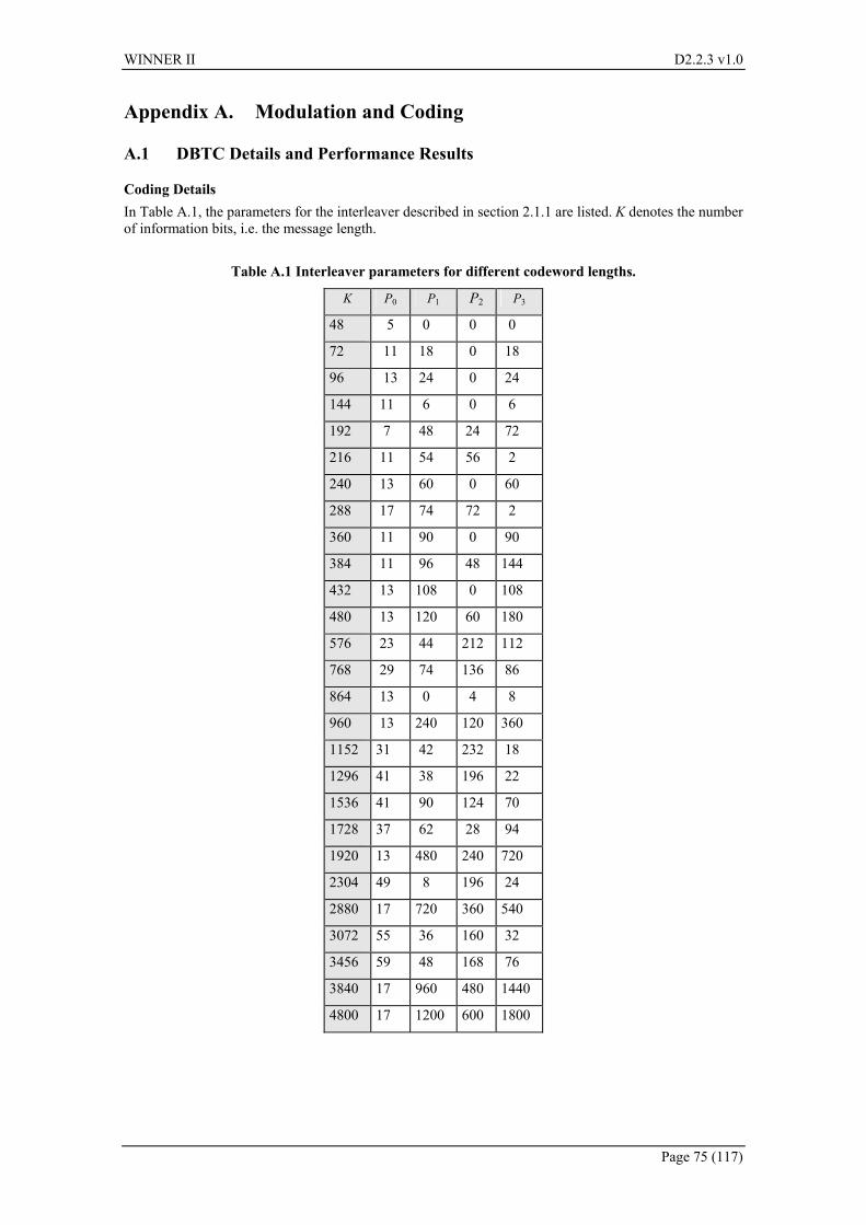
WINNER II D2.2.3 v1.0
Page 75 (117)
Appendix A. Modulation and Coding
A.1 DBTC Details and Performance Results
Coding Details In Table A.1, the parameters for the interleaver described in section 2.1.1 are listed. K denotes the number of information bits, i.e. the message length.
Table A.1 Interleaver parameters for different codeword lengths.
K P0 P1 P2 P3
48 5 0 0 0
72 11 18 0 18
96 13 24 0 24
144 11 6 0 6
192 7 48 24 72
216 11 54 56 2
240 13 60 0 60
288 17 74 72 2
360 11 90 0 90
384 11 96 48 144
432 13 108 0 108
480 13 120 60 180
576 23 44 212 112
768 29 74 136 86
864 13 0 4 8
960 13 240 120 360
1152 31 42 232 18
1296 41 38 196 22
1536 41 90 124 70
1728 37 62 28 94
1920 13 480 240 720
2304 49 8 196 24
2880 17 720 360 540
3072 55 36 160 32
3456 59 48 168 76
3840 17 960 480 1440
4800 17 1200 600 1800

WINNER II D2.2.3 v1.0
Page 76 (117)
Table A.2 lists the parameters α and 0γ which are required for the numerical approximation of the CWER curves for all considered combinations of the message length K, the number of bits per symbol b and the code rate R.
Table A.2 Parameters α and 0γ for approximation of CWER curves with (2.6).
K b R α 10 lg(γth) K b R α 10 lg(γth)
2 1/3 21.1525 -1.47 dB 2 1/3 37.3454 -1.34 dB 2 2/5 17.7710 -0.50 dB 2 2/5 28.6631 -0.46 dB 2 1/2 13.0877 0.75 dB 2 1/2 22.7759 0.87 dB 2 4/7 10.5338 1.68 dB 2 4/7 17.4025 1.71 dB 2 2/3 7.3723 2.73 dB 2 2/3 13.5356 2.79 dB 2 3/4 5.0264 3.71 dB 2 3/4 9.8805 3.89 dB 2 4/5 4.0337 4.30 dB 2 4/5 7.8614 4.52 dB 2 6/7 2.8135 5.07 dB 2 6/7 4.9148 5.31 dB 4 1/3 6.0820 3.31 dB 4 1/3 10.7319 3.41 dB 4 2/5 4.8686 4.46 dB 4 2/5 8.4153 4.53 dB 4 1/2 3.2201 5.96 dB 4 1/2 5.8436 6.11 dB 4 4/7 2.4331 7.12 dB 4 4/7 4.1306 7.16 dB 4 2/3 1.6545 8.50 dB 4 2/3 3.2371 8.63 dB 4 3/4 1.0728 9.69 dB 4 3/4 2.1561 9.90 dB 4 4/5 0.8642 10.46 dB 4 4/5 1.6916 10.68 dB 4 6/7 0.5777 11.30 dB 4 6/7 0.9705 11.54 dB 6 1/3 2.2671 7.08 dB 6 1/3 4.1137 7.15 dB 6 2/5 1.5902 8.32 dB 6 2/5 2.9282 8.50 dB 6 1/2 1.0273 10.32 dB 6 1/2 1.8349 10.43 dB 6 4/7 0.7162 11.69 dB 6 4/7 1.2743 11.75 dB 6 2/3 0.4407 13.35 dB 6 2/3 0.9115 13.53 dB 6 3/4 0.2815 14.90 dB 6 3/4 0.5582 15.09 dB 6 4/5 0.2223 15.85 dB 6 4/5 0.4321 16.04 dB 6 6/7 0.1448 16.86 dB 6 6/7 0.2554 17.09 dB 8 1/3 0.8506 10.16 dB 8 1/3 1.5974 10.32 dB 8 2/5 0.6093 12.03 dB 8 2/5 1.1152 12.09 dB 8 1/2 0.3410 14.35 dB 8 1/2 0.6524 14.51 dB 8 4/7 0.2203 15.94 dB 8 4/7 0.4343 16.13 dB 8 2/3 0.1301 18.04 dB 8 2/3 0.2754 18.22 dB 8 3/4 0.0742 19.76 dB 8 3/4 0.1577 20.08 dB 8 4/5 0.0569 20.90 dB 8 4/5 0.1109 21.15 dB
288
8 6/7 0.0361 22.09 dB
1152
8 6/7 0.0652 22.44 dB

WINNER II D2.2.3 v1.0
Page 77 (117)
Performance Results
2 4 6 8 10 12 1410
-4
10-3
10-2
10-1
100
ES/N0 [dB]
CW
ER
Duo-binary turbo codes, K = 288, 1152. b = 4
R = 1/3R = 2/5R = 1/2R = 4/7R = 2/3R = 3/4R = 4/5R = 6/7
Figure A.1 CWER curves for 16-QAM. Continuous lines: K = 288, dashed lines: K = 1152
4 6 8 10 12 14 16 18 2010
-4
10-3
10-2
10-1
100
ES/N0 [dB]
CW
ER
Duo-binary turbo codes, K = 288, 1152. b = 6
R = 1/3R = 2/5R = 1/2R = 4/7R = 2/3R = 3/4R = 4/5R = 6/7
Figure A.2 CWER curves for 64-QAM. Continuous lines: K = 288, dashed lines: K = 1152

WINNER II D2.2.3 v1.0
Page 78 (117)
8 10 12 14 16 18 20 22 24 2610
-4
10-3
10-2
10-1
100
ES/N0 [dB]
CW
ER
Duo-binary turbo codes, K = 288, 1152. b = 8
R = 1/3R = 2/5R = 1/2R = 4/7R = 2/3R = 3/4R = 4/5R = 6/7
Figure A.3 CWER curves for 256-QAM. Continuous lines: K = 288, dashed lines: K = 1152
A.2 RCP BLDPC Performance Results Please note that the results presented in Figure 2.15 and in Appendix A.2 are plotted against 0/ NEb [dB]. To obtain SNR thresholds, like the ones presented in Table 3.8 and Table 3.9, each curve needs to be shifted by the following value (in dB scale):
)(log10 10 bRx ⋅= (A.1)
BPSK and QPSK curves are identical, assuming 0/ NEb arguments, so only one plot is included for both.
Figure A.4 CWER curves for 16-QAM and K = 288

WINNER II D2.2.3 v1.0
Page 79 (117)
Figure A.5 CWER curves for 64-QAM and K = 288
Figure A.6: CWER curves for 256-QAM and K = 288

WINNER II D2.2.3 v1.0
Page 80 (117)
Figure A.7: CWER curves for QPSK (and BPSK) and K = 1152
Figure A.8: CWER curves for 16-QAM and K = 1152

WINNER II D2.2.3 v1.0
Page 81 (117)
Figure A.9: CWER curves for 64-QAM and K = 1152
Figure A.10: CWER curves for 256-QAM and K = 1152

WINNER II D2.2.3 v1.0
Page 82 (117)
A.3 Base Matrix for R = ½ RCP BLDPC Code
Table A.3: Transposed base matrix of R = 1/2 rate compatible punctured BLDPC code
-1 65 10 -1 11 63 52 90 -1 30 -1 49 -1 -1 -1 -1 94 -1 -1 92 61 -1 -1 76 60 -1 4 26 -1 -1 -1 38 0 -1 -1 -1 66 1 -1 -1 86 70 -1 -1 73 55 28 -1 -1 7 -1 16 -1 73 89 -1 -1 -1 -1 10 37 -1 3 62 -1 7 29 3 -1 25 -1 -1 -1 -1 -1 -1 13 52 86 -1 -1 42 87 70 -1 78 69 -1 27 -1 -1 64 5 -1 -1 71 14 -1 52 18 3 -1 -1 71 73 91 -1 -1 9 -1 -1 72 -1 -1 5 -1 -1 29 59 -1 -1 7 -1 9 -1 -1 -1 -1 -1 -1 30 4 -1 19 42 -1 38 83 28 -1 12 34 -1 21 -1 -1 28 -1 58 78 -1 64 46 47 14 -1 5 -1 -1 85 -1 27 -1 53 -1 -1 77 -1 5 -1 -1 -1 -1 -1 9 -1 -1 -1 -1 -1 -1 -1 -1 -1 -1 -1 -1 -1 -1 -1 -1 52 -1 31 -1 -1 -1 -1 -1 -1 36 -1 -1 -1 -1 -1 -1 -1 58 -1 -1 -1 -1 -1 -1 -1 51 -1 -1 -1 -1 -1 -1 -1 -1 -1 -1 -1 -1 38 -1 -1 -1 -1 -1 8 -1 -1 -1 -1 -1 -1 -1 -1 -1 -1 -1 -1 -1 -1 -1 78 -1 -1 -1 -1 -1 26 -1 -1 -1 -1 -1 8 -1 -1 -1 -1 -1 63 -1 -1 -1 -1 -1 -1 35 -1 -1 -1 -1 -1 -1 -1 46 -1 -1 -1 -1 -1 1 94 -1 -1 -1 -1 -1 -1 -1 -1 -1 -1 -1 -1 -1 -1 -1 -1 -1 6 -1 -1 -1 -1 -1 -1 -1 -1 53 -1 -1 -1 -1 -1 -1 -1 -1 64 -1 -1 -1 -1 -1 -1 77 -1 -1 17 -1 -1 8 -1 -1 -1 -1 -1 5 -1 -1 -1 -1 -1 -1 -1 -1 -1 -1 -1 -1 -1 -1 -1 -1 -1 -1 -1 -1 9 -1 48 -1 -1 -1 -1 -1 -1 -1 -1 45 -1 -1 -1 -1 -1 57 -1 -1 -1 -1 -1 -1 -1 -1 -1 -1 -1 -1 -1 57 28 -1 -1 -1 -1 -1 -1 -1 -1 -1 30 -1 -1 -1 -1 -1 -1 -1 -1 43 -1 -1 11 -1 -1 -1 -1 -1 -1 -1 -1 -1 -1 -1 -1 -1 -1 -1 -1 -1 -1 19 -1 -1 -1 -1 -1 -1 -1 -1 -1 20 -1 89 -1 -1 -1 -1 -1 -1 -1 -1 -1 -1 71 -1 -1 -1 -1 -1 -1 -1 -1 66 -1 -1 -1 -1 -1 16 -1 -1 -1 -1 41 -1 -1 -1 -1 -1 -1 -1 -1 -1 -1 -1 -1 -1 -1 -1 -1 -1 93 -1 3 -1 -1 -1 -1 68 -1 29 -1 -1 -1 -1 -1 23 -1 -1 -1 -1 -1 -1 -1 -1 -1 -1 -1 -1 -1 53 -1 -1 -1 -1 -1 -1 93 -1 55 -1 -1 -1 -1 -1 -1 -1 -1 -1 -1 -1 -1 -1 -1 -1 -1 -1 65 -1 -1 -1 -1 -1 -1 -1 -1 -1 -1 -1 25 -1 8 -1 -1 -1 -1 1 -1 -1 -1 -1 -1 -1 -1 -1 -1 -1 -1 -1 -1 82 -1 -1 -1 -1 -1 -1 -1 -1 55 0 0 -1 -1 -1 -1 -1 -1 -1 -1 -1 -1 -1 -1 -1 -1 -1 -1 -1 -1 -1 -1 -1 -1 -1 0 0 -1 -1 -1 -1 -1 -1 -1 -1 -1 -1 -1 -1 -1 -1 -1 -1 -1 -1 -1 -1 -1 -1 -1 0 0 -1 -1 -1 -1 -1 -1 -1 -1 -1 -1 -1 -1 -1 -1 -1 -1 -1 -1 -1 -1 -1 -1 -1 0 0 -1 -1 -1 -1 -1 -1 -1 -1 -1 -1 -1 -1 -1 -1 -1 -1 -1 -1 -1 -1 -1 -1 -1 0 0 -1 -1 -1 -1 -1 -1 -1 -1 -1 -1 -1 -1 -1 -1 -1 -1 -1 -1 -1 -1 -1 -1 -1 0 0 -1 -1 -1 -1 -1 -1 -1 -1 -1 -1 -1 -1 -1 -1 -1 -1 -1 -1 -1 -1 -1 -1 -1 0 0 -1 -1 -1 -1 -1 -1 -1 -1 -1 -1 -1 -1 -1 -1 -1 -1 -1 -1 -1 -1 -1 -1 -1 0 0 -1 -1 -1 -1 -1 -1 -1 -1 -1 -1 -1 -1 -1 -1 -1 -1 -1 -1 -1 -1 -1 -1 -1 0 0 -1 -1 -1 -1 -1 -1 -1 -1 -1 -1 -1 -1 -1 -1 -1 -1 -1 -1 -1 -1 -1 -1 -1 0 0 -1 -1 -1 -1 -1 -1 -1 -1 -1 -1 -1 -1 -1 -1 -1 -1 -1 -1 -1 -1 -1 -1 -1 0 0 -1 -1 -1 -1 -1 -1 -1 -1 -1 -1 -1 -1 -1 -1 -1 -1 -1 -1 -1 -1 -1 -1 -1 0 0 -1 -1 -1 -1 -1 -1 -1 -1 -1 -1 -1 -1 -1 -1 -1 -1 -1 -1 -1 -1 -1 -1 -1 0 0 -1 -1 -1 -1 -1 -1 -1 -1 -1 -1 -1 -1 -1 -1 -1 -1 -1 -1 -1 -1 -1 -1 -1 0 0 -1 -1 -1 -1 -1 -1 -1 -1 -1 -1 -1 -1 -1 -1 -1 -1 -1 -1 -1 -1 -1 -1 -1 0 0 -1 -1 -1 -1 -1 -1 -1 -1 -1 -1 -1 -1 -1 -1 -1 -1 -1 -1 -1 -1 -1 -1 -1 0 0 -1 -1 -1 -1 -1 -1 -1 -1 -1 -1 -1 -1 -1 -1 -1 -1 -1 -1 -1 -1 -1 -1 -1 0 0 -1 -1 -1 -1 -1 -1 -1 -1 -1 -1 -1 -1 -1 -1 -1 -1 -1 -1 -1 -1 -1 -1 -1 0 0 -1 -1 -1 -1 -1 -1 -1 -1 -1 -1 -1 -1 -1 -1 -1 -1 -1 -1 -1 -1 -1 -1 -1 0 0 -1 -1 -1 -1 -1 -1 -1 -1 -1 -1 -1 -1 -1 -1 -1 -1 -1 -1 -1 -1 -1 -1 -1 0 0 -1 -1 -1 -1 -1 -1 -1 -1 -1 -1 -1 -1 -1 -1 -1 -1 -1 -1 -1 -1 -1 -1 -1 0 0 -1 -1 -1 -1 -1 -1 -1 -1 -1 -1 -1 -1 -1 -1 -1 -1 -1 -1 -1 -1 -1 -1 -1 0 0 -1 -1 -1 -1 -1 -1 -1 -1 -1 -1 -1 -1 -1 -1 -1 -1 -1 -1 -1 -1 -1 -1 -1 0 0
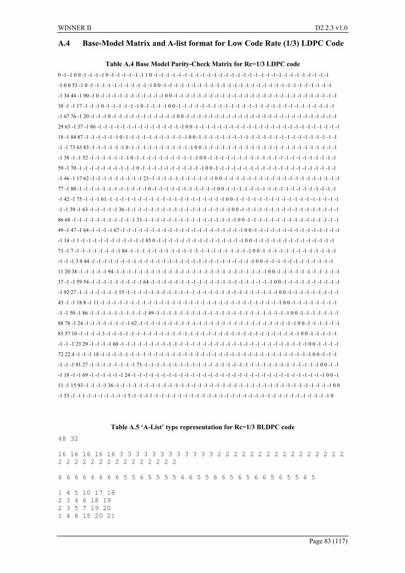
WINNER II D2.2.3 v1.0
Page 83 (117)
A.4 Base-Model Matrix and A-list format for Low Code Rate (1/3) LDPC Code
Table A.4 Base Model Parity-Check Matrix for Rc=1/3 LDPC code 0 -1 -1 0 0 -1 -1 -1 -1 0 -1 -1 -1 -1 -1 -1 1 0 -1 -1 -1 -1 -1 -1 -1 -1 -1 -1 -1 -1 -1 -1 -1 -1 -1 -1 -1 -1 -1 -1 -1 -1 -1 -1 -1 -1 -1 -1
-1 0 0 53 -1 0 -1 -1 -1 -1 -1 -1 -1 -1 -1 -1 -1 0 0 -1 -1 -1 -1 -1 -1 -1 -1 -1 -1 -1 -1 -1 -1 -1 -1 -1 -1 -1 -1 -1 -1 -1 -1 -1 -1 -1 -1 -1
-1 34 44 -1 90 -1 0 -1 -1 -1 -1 -1 -1 -1 -1 -1 -1 -1 0 0 -1 -1 -1 -1 -1 -1 -1 -1 -1 -1 -1 -1 -1 -1 -1 -1 -1 -1 -1 -1 -1 -1 -1 -1 -1 -1 -1 -1
38 -1 -1 17 -1 -1 -1 0 -1 -1 -1 -1 -1 -1 0 -1 -1 -1 -1 0 0 -1 -1 -1 -1 -1 -1 -1 -1 -1 -1 -1 -1 -1 -1 -1 -1 -1 -1 -1 -1 -1 -1 -1 -1 -1 -1 -1
-1 67 76 -1 20 -1 -1 -1 0 -1 -1 -1 -1 -1 -1 -1 -1 -1 -1 -1 0 0 -1 -1 -1 -1 -1 -1 -1 -1 -1 -1 -1 -1 -1 -1 -1 -1 -1 -1 -1 -1 -1 -1 -1 -1 -1 -1
29 63 -1 37 -1 86 -1 -1 -1 -1 -1 -1 -1 -1 -1 -1 -1 -1 -1 -1 -1 0 0 -1 -1 -1 -1 -1 -1 -1 -1 -1 -1 -1 -1 -1 -1 -1 -1 -1 -1 -1 -1 -1 -1 -1 -1 -1
18 -1 84 87 -1 -1 -1 -1 -1 -1 0 -1 -1 -1 -1 -1 -1 -1 -1 -1 -1 -1 0 0 -1 -1 -1 -1 -1 -1 -1 -1 -1 -1 -1 -1 -1 -1 -1 -1 -1 -1 -1 -1 -1 -1 -1 -1
-1 -1 73 63 83 -1 -1 -1 -1 -1 -1 0 -1 -1 -1 -1 -1 -1 -1 -1 -1 -1 -1 0 0 -1 -1 -1 -1 -1 -1 -1 -1 -1 -1 -1 -1 -1 -1 -1 -1 -1 -1 -1 -1 -1 -1 -1
-1 38 -1 -1 52 -1 -1 -1 -1 -1 -1 -1 0 -1 -1 -1 -1 -1 -1 -1 -1 -1 -1 -1 0 0 -1 -1 -1 -1 -1 -1 -1 -1 -1 -1 -1 -1 -1 -1 -1 -1 -1 -1 -1 -1 -1 -1
59 -1 70 -1 -1 -1 -1 -1 -1 -1 -1 -1 -1 0 -1 -1 -1 -1 -1 -1 -1 -1 -1 -1 -1 0 0 -1 -1 -1 -1 -1 -1 -1 -1 -1 -1 -1 -1 -1 -1 -1 -1 -1 -1 -1 -1 -1
-1 46 -1 17 62 -1 -1 -1 -1 -1 -1 -1 -1 -1 23 -1 -1 -1 -1 -1 -1 -1 -1 -1 -1 -1 0 0 -1 -1 -1 -1 -1 -1 -1 -1 -1 -1 -1 -1 -1 -1 -1 -1 -1 -1 -1 -1
77 -1 80 -1 -1 -1 -1 -1 -1 -1 -1 -1 -1 -1 -1 0 -1 -1 -1 -1 -1 -1 -1 -1 -1 -1 -1 0 0 -1 -1 -1 -1 -1 -1 -1 -1 -1 -1 -1 -1 -1 -1 -1 -1 -1 -1 -1
-1 42 -1 75 -1 -1 -1 61 -1 -1 -1 -1 -1 -1 -1 -1 -1 -1 -1 -1 -1 -1 -1 -1 -1 -1 -1 -1 0 0 -1 -1 -1 -1 -1 -1 -1 -1 -1 -1 -1 -1 -1 -1 -1 -1 -1 -1
-1 -1 39 -1 63 -1 -1 -1 -1 -1 36 -1 -1 -1 -1 -1 -1 -1 -1 -1 -1 -1 -1 -1 -1 -1 -1 -1 -1 0 0 -1 -1 -1 -1 -1 -1 -1 -1 -1 -1 -1 -1 -1 -1 -1 -1 -1
86 68 -1 -1 -1 -1 -1 -1 -1 -1 -1 -1 -1 33 -1 -1 -1 -1 -1 -1 -1 -1 -1 -1 -1 -1 -1 -1 -1 -1 0 0 -1 -1 -1 -1 -1 -1 -1 -1 -1 -1 -1 -1 -1 -1 -1 -1
49 -1 47 -1 64 -1 -1 -1 -1 67 -1 -1 -1 -1 -1 -1 -1 -1 -1 -1 -1 -1 -1 -1 -1 -1 -1 -1 -1 -1 -1 0 0 -1 -1 -1 -1 -1 -1 -1 -1 -1 -1 -1 -1 -1 -1 -1
-1 14 -1 1 -1 -1 -1 -1 -1 -1 -1 -1 -1 -1 -1 85 0 -1 -1 -1 -1 -1 -1 -1 -1 -1 -1 -1 -1 -1 -1 -1 0 0 -1 -1 -1 -1 -1 -1 -1 -1 -1 -1 -1 -1 -1 -1
73 -1 7 -1 -1 -1 -1 -1 -1 -1 -1 84 -1 -1 -1 -1 -1 -1 -1 -1 -1 -1 -1 -1 -1 -1 -1 -1 -1 -1 -1 -1 -1 0 0 -1 -1 -1 -1 -1 -1 -1 -1 -1 -1 -1 -1 -1
-1 -1 -1 3 8 44 -1 -1 -1 -1 -1 -1 -1 -1 -1 -1 -1 -1 -1 -1 -1 -1 -1 -1 -1 -1 -1 -1 -1 -1 -1 -1 -1 -1 0 0 -1 -1 -1 -1 -1 -1 -1 -1 -1 -1 -1 -1
11 20 38 -1 -1 -1 -1 -1 94 -1 -1 -1 -1 -1 -1 -1 -1 -1 -1 -1 -1 -1 -1 -1 -1 -1 -1 -1 -1 -1 -1 -1 -1 -1 -1 0 0 -1 -1 -1 -1 -1 -1 -1 -1 -1 -1 -1
37 -1 -1 59 54 -1 -1 -1 -1 -1 -1 -1 -1 -1 64 -1 -1 -1 -1 -1 -1 -1 -1 -1 -1 -1 -1 -1 -1 -1 -1 -1 -1 -1 -1 -1 0 0 -1 -1 -1 -1 -1 -1 -1 -1 -1 -1
-1 92 27 -1 -1 -1 -1 -1 -1 -1 15 -1 -1 -1 -1 -1 -1 -1 -1 -1 -1 -1 -1 -1 -1 -1 -1 -1 -1 -1 -1 -1 -1 -1 -1 -1 -1 0 0 -1 -1 -1 -1 -1 -1 -1 -1 -1
43 -1 -1 18 8 -1 11 -1 -1 -1 -1 -1 -1 -1 -1 -1 -1 -1 -1 -1 -1 -1 -1 -1 -1 -1 -1 -1 -1 -1 -1 -1 -1 -1 -1 -1 -1 -1 0 0 -1 -1 -1 -1 -1 -1 -1 -1
-1 -1 50 -1 86 -1 -1 -1 -1 -1 -1 -1 -1 -1 -1 49 -1 -1 -1 -1 -1 -1 -1 -1 -1 -1 -1 -1 -1 -1 -1 -1 -1 -1 -1 -1 -1 -1 -1 0 0 -1 -1 -1 -1 -1 -1 -1
88 78 -1 24 -1 -1 -1 -1 -1 -1 -1 -1 62 -1 -1 -1 -1 -1 -1 -1 -1 -1 -1 -1 -1 -1 -1 -1 -1 -1 -1 -1 -1 -1 -1 -1 -1 -1 -1 -1 0 0 -1 -1 -1 -1 -1 -1
83 57 10 -1 -1 -1 -1 3 -1 -1 -1 -1 -1 -1 -1 -1 -1 -1 -1 -1 -1 -1 -1 -1 -1 -1 -1 -1 -1 -1 -1 -1 -1 -1 -1 -1 -1 -1 -1 -1 -1 0 0 -1 -1 -1 -1 -1
-1 -1 -1 23 29 -1 -1 -1 -1 60 -1 -1 -1 -1 -1 -1 -1 -1 -1 -1 -1 -1 -1 -1 -1 -1 -1 -1 -1 -1 -1 -1 -1 -1 -1 -1 -1 -1 -1 -1 -1 -1 0 0 -1 -1 -1 -1
72 22 4 -1 -1 -1 18 -1 -1 -1 -1 -1 -1 -1 -1 -1 -1 -1 -1 -1 -1 -1 -1 -1 -1 -1 -1 -1 -1 -1 -1 -1 -1 -1 -1 -1 -1 -1 -1 -1 -1 -1 -1 0 0 -1 -1 -1
-1 -1 -1 91 27 -1 -1 -1 -1 -1 -1 -1 -1 75 -1 -1 -1 -1 -1 -1 -1 -1 -1 -1 -1 -1 -1 -1 -1 -1 -1 -1 -1 -1 -1 -1 -1 -1 -1 -1 -1 -1 -1 -1 0 0 -1 -1
-1 18 -1 -1 69 -1 -1 -1 -1 -1 -1 24 -1 -1 -1 -1 -1 -1 -1 -1 -1 -1 -1 -1 -1 -1 -1 -1 -1 -1 -1 -1 -1 -1 -1 -1 -1 -1 -1 -1 -1 -1 -1 -1 -1 0 0 -1
11 -1 15 93 -1 -1 -1 -1 36 -1 -1 -1 -1 -1 -1 -1 -1 -1 -1 -1 -1 -1 -1 -1 -1 -1 -1 -1 -1 -1 -1 -1 -1 -1 -1 -1 -1 -1 -1 -1 -1 -1 -1 -1 -1 -1 0 0
-1 53 -1 -1 1 -1 -1 -1 -1 -1 -1 -1 5 -1 -1 -1 1 -1 -1 -1 -1 -1 -1 -1 -1 -1 -1 -1 -1 -1 -1 -1 -1 -1 -1 -1 -1 -1 -1 -1 -1 -1 -1 -1 -1 -1 -1 0
Table A.5 ‘A-List’ type representation for Rc=1/3 BLDPC code
48 32 16 16 16 16 16 3 3 3 3 3 3 3 3 3 3 3 3 2 2 2 2 2 2 2 2 2 2 2 2 2 2 2 2 2 2 2 2 2 2 2 2 2 2 2 2 2 2 2 6 6 6 6 6 6 6 6 5 5 6 5 5 5 5 6 6 5 5 6 6 5 6 5 6 6 5 6 5 5 6 5 1 4 5 10 17 18 2 3 4 6 18 19 2 3 5 7 19 20 1 4 8 15 20 21

WINNER II D2.2.3 v1.0
Page 84 (117)
2 3 5 9 21 22 1 2 4 6 22 23 1 3 4 11 23 24 3 4 5 12 24 25 2 5 13 25 26 1 3 14 26 27 2 4 5 15 27 28 1 3 16 28 29 2 4 8 29 30 3 5 11 30 31 1 2 14 31 32 1 3 5 10 32 33 2 4 16 17 33 34 1 3 12 34 35 4 5 6 35 36 1 2 3 9 36 37 1 4 5 15 37 38 2 3 11 38 39 1 4 5 7 39 40 3 5 16 40 41 1 2 4 13 41 42 1 2 3 8 42 43 4 5 10 43 44 1 2 3 7 44 45 4 5 14 45 46 2 5 12 46 47 1 3 4 9 47 48 2 5 13 17 48 0 0 0 0 1 0 0 0 53 0 0 0 34 44 90 0 0 0 38 17 0 0 0 0 67 76 20 0 0 0 29 63 37 86 0 0 18 84 87 0 0 0 73 63 83 0 0 0 38 52 0 0 0 59 70 0 0 0 46 17 62 23 0 0 77 80 0 0 0 42 75 61 0 0 39 63 36 0 0 86 68 33 0 0 49 47 64 67 0 0 14 1 85 0 0 0 73 7 84 0 0 3 8 44 0 0 11 20 38 94 0 0 37 59 54 64 0 0 92 27 15 0 0 43 18 8 11 0 0 50 86 49 0 0 88 78 24 62 0 0 83 57 10 3 0 0 23 29 60 0 0 72 22 4 18 0 0 91 27 75 0 0 18 69 24 0 0 11 15 93 36 0 0 53 1 5 1 0

WINNER II D2.2.3 v1.0
Page 85 (117)
A.5 Performance Results for Low-Code Rate (1/3) BLDPC Code In this part of annex, full performance results (BER, CWER, Average number of iterations) are provided for the agreed 2 data information length of special interest, namely K=288, and K=1152, whilst varying modulation format from QPSK, 16-QAM, 64-QAM and 256-QAM (used in Local Area Network scenarios).
0 2 4 6 8 10 1210-8
10-7
10-6
10-5
10-4
10-3
10-2
10-1
100
Eb/N0 (dB)
BER
Zf=18, N=864, MSA* (0.8), Horizontal Scheduling, AWGN
QPSK16-QAM64-QAM256-QAM
Figure A.11 BER results for K = 288 (Zf=18) with R = 1/3 BLDPCC over AWGN
0 2 4 6 8 10 1210-5
10-4
10-3
10-2
10-1
100
Eb/N0 (dB)
CW
ER
Zf=18, N=864, MSA* (0.8), Horizontal Scheduling, AWGN
QPSK16-QAM64-QAM256-QAM
Figure A.12 CWER for K = 288 (Zf=18) with R = 1/3 BLDPCC over AWGN

WINNER II D2.2.3 v1.0
Page 86 (117)
10-8 10-7 10-6 10-5 10-4 10-3 10-2 10-1 1000
5
10
15
20
25
BER
Nite
r
Niter Vs BER, MSA* (0.8), Horizontal Scheduling, Zf=18, N=864, AWGN
QPSK16-QAM64-QAM256-QAM
Figure A.13 Average number of iterations w.r.t. BER and M-QAM, K=288, R = 1/3, (Zf=18)
It’s worth mentioning the fast decrease of the average number of iterations w.r.t. BER, and thus SNR increase. This is particularly true whilst using Layered BP processing, e.g. Horizontal scheduling. In our case, due to specific nature and structure of designed LDPC codes, we are using a Group-Layered BP, to take fully advantage of the parallelism benefit of LDPC codes.
0 1 2 3 4 5 6 7 8 9 1010-8
10-7
10-6
10-5
10-4
10-3
10-2
10-1
100
Eb/N0 (dB)
BER
Zf=72, N=3456, MSA* (0.8), Horizontal Scheduling, AWGN
QPSK16-QAM64-QAM256-QAM
Figure A.14 BER results for K = 1152 (Zf=72) with R = 1/3 BLDPCC over AWGN

WINNER II D2.2.3 v1.0
Page 87 (117)
0 1 2 3 4 5 6 7 8 9 1010-5
10-4
10-3
10-2
10-1
100
Eb/N0 (dB)
CW
ER
Zf=72, N=3456, MSA* (0.8), Horizontal Scheduling, AWGN
QPSK16-QAM64-QAM256-QAM
Figure A.15 CWER results for K = 1152 (Zf=72) with R = 1/3 BLDPCC over AWGN
10-8 10-7 10-6 10-5 10-4 10-3 10-2 10-1 1000
5
10
15
20
25
BER
Nite
r
Niter Vs BER, MSA* (0.8), Horizontal Scheduling, Zf=72, N=3456, AWGN
QPSK16-QAM64-QAM256-QAM
Figure A.16 Average number of iterations w.r.t. BER and M-QAM, K = 1152, R = 1/3, (Zf=72)

WINNER II D2.2.3 v1.0
Page 88 (117)
A.6 Lifted base-matrices for QC-BLDPC Codes
R = 1/3
Table A.6 Lifted Base-model parity-check matrix, R = 1/3 QC-BLDPC Code 0 -1 -1 38 -1 413 210 -1 -1 59 -1 269 -1 -1 182 337 -1 169 -1 491 229 -1 331 -1 568 275 -1 72 -1 -1 395 -1
-1 0 322 -1 547 63 -1 -1 230 -1 526 -1 522 -1 452 -1 110 -1 -1 500 -1 572 -1 -1 366 57 -1 118 -1 18 -1 53
-1 0 140 -1 76 -1 84 73 -1 262 -1 176 -1 39 -1 527 -1 295 -1 230 -1 219 -1 146 -1 394 -1 196 -1 -1 495 -1
0 53 -1 305 -1 325 279 351 -1 -1 209 -1 267 -1 -1 -1 97 -1 99 -1 347 -1 18 -1 120 -1 503 -1 91 -1 573 -1
0 -1 570 -1 116 -1 -1 275 532 -1 62 -1 -1 159 -1 448 -1 -1 104 -1 54 -1 200 86 -1 -1 413 -1 411 69 -1 289
-1 0 -1 -1 -1 566 -1 -1 -1 -1 -1 -1 -1 -1 -1 -1 -1 -1 140 -1 -1 -1 -1 -1 -1 -1 -1 -1 -1 -1 -1 -1
-1 -1 0 -1 -1 -1 -1 -1 -1 -1 -1 -1 -1 -1 -1 -1 -1 -1 -1 -1 -1 -1 299 -1 -1 -1 -1 210 -1 -1 -1 -1
-1 -1 -1 0 -1 -1 -1 -1 -1 -1 -1 -1 157 -1 -1 -1 -1 -1 -1 -1 -1 -1 -1 -1 -1 483 -1 -1 -1 -1 -1 -1
-1 -1 -1 -1 0 -1 -1 -1 -1 -1 -1 -1 -1 -1 -1 -1 -1 -1 -1 94 -1 -1 -1 -1 -1 -1 -1 -1 -1 -1 516 -1
0 -1 -1 -1 -1 -1 -1 -1 -1 -1 -1 -1 -1 -1 -1 451 -1 -1 -1 -1 -1 -1 -1 -1 -1 -1 252 -1 -1 -1 -1 -1
-1 -1 -1 -1 -1 -1 0 -1 -1 -1 -1 -1 -1 132 -1 -1 -1 -1 -1 -1 -1 15 -1 -1 -1 -1 -1 -1 -1 -1 -1 -1
-1 -1 -1 -1 -1 -1 -1 0 -1 -1 -1 -1 -1 -1 -1 -1 -1 180 -1 -1 -1 -1 -1 -1 -1 -1 -1 -1 -1 24 -1 -1
-1 -1 -1 -1 -1 -1 -1 -1 0 -1 -1 -1 -1 -1 -1 -1 -1 -1 -1 -1 -1 -1 -1 -1 446 -1 -1 -1 -1 -1 -1 389
-1 -1 -1 -1 -1 -1 -1 -1 -1 0 -1 -1 -1 -1 129 -1 -1 -1 -1 -1 -1 -1 -1 -1 -1 -1 -1 -1 363 -1 -1 -1
-1 -1 -1 0 -1 -1 -1 -1 -1 -1 407 -1 -1 -1 -1 -1 -1 -1 -1 -1 544 -1 -1 -1 -1 -1 -1 -1 -1 -1 -1 -1
-1 -1 -1 -1 -1 -1 -1 -1 -1 -1 -1 0 -1 -1 -1 -1 565 -1 -1 -1 -1 -1 -1 241 -1 -1 -1 -1 -1 -1 -1 -1
1 -1 -1 -1 -1 -1 -1 -1 -1 -1 -1 -1 -1 -1 -1 -1 0 -1 -1 -1 -1 -1 -1 -1 -1 -1 -1 -1 -1 -1 -1 1
0 0 -1 -1 -1 -1 -1 -1 -1 -1 -1 -1 -1 -1 -1 -1 -1 -1 -1 -1 -1 -1 -1 -1 -1 -1 -1 -1 -1 -1 -1 -1
-1 0 0 -1 -1 -1 -1 -1 -1 -1 -1 -1 -1 -1 -1 -1 -1 -1 -1 -1 -1 -1 -1 -1 -1 -1 -1 -1 -1 -1 -1 -1
-1 -1 0 0 -1 -1 -1 -1 -1 -1 -1 -1 -1 -1 -1 -1 -1 -1 -1 -1 -1 -1 -1 -1 -1 -1 -1 -1 -1 -1 -1 -1
-1 -1 -1 0 0 -1 -1 -1 -1 -1 -1 -1 -1 -1 -1 -1 -1 -1 -1 -1 -1 -1 -1 -1 -1 -1 -1 -1 -1 -1 -1 -1
-1 -1 -1 -1 0 0 -1 -1 -1 -1 -1 -1 -1 -1 -1 -1 -1 -1 -1 -1 -1 -1 -1 -1 -1 -1 -1 -1 -1 -1 -1 -1
-1 -1 -1 -1 -1 0 0 -1 -1 -1 -1 -1 -1 -1 -1 -1 -1 -1 -1 -1 -1 -1 -1 -1 -1 -1 -1 -1 -1 -1 -1 -1
-1 -1 -1 -1 -1 -1 0 0 -1 -1 -1 -1 -1 -1 -1 -1 -1 -1 -1 -1 -1 -1 -1 -1 -1 -1 -1 -1 -1 -1 -1 -1
-1 -1 -1 -1 -1 -1 -1 0 0 -1 -1 -1 -1 -1 -1 -1 -1 -1 -1 -1 -1 -1 -1 -1 -1 -1 -1 -1 -1 -1 -1 -1
-1 -1 -1 -1 -1 -1 -1 -1 0 0 -1 -1 -1 -1 -1 -1 -1 -1 -1 -1 -1 -1 -1 -1 -1 -1 -1 -1 -1 -1 -1 -1
-1 -1 -1 -1 -1 -1 -1 -1 -1 0 0 -1 -1 -1 -1 -1 -1 -1 -1 -1 -1 -1 -1 -1 -1 -1 -1 -1 -1 -1 -1 -1
-1 -1 -1 -1 -1 -1 -1 -1 -1 -1 0 0 -1 -1 -1 -1 -1 -1 -1 -1 -1 -1 -1 -1 -1 -1 -1 -1 -1 -1 -1 -1
-1 -1 -1 -1 -1 -1 -1 -1 -1 -1 -1 0 0 -1 -1 -1 -1 -1 -1 -1 -1 -1 -1 -1 -1 -1 -1 -1 -1 -1 -1 -1
-1 -1 -1 -1 -1 -1 -1 -1 -1 -1 -1 -1 0 0 -1 -1 -1 -1 -1 -1 -1 -1 -1 -1 -1 -1 -1 -1 -1 -1 -1 -1
-1 -1 -1 -1 -1 -1 -1 -1 -1 -1 -1 -1 -1 0 0 -1 -1 -1 -1 -1 -1 -1 -1 -1 -1 -1 -1 -1 -1 -1 -1 -1
-1 -1 -1 -1 -1 -1 -1 -1 -1 -1 -1 -1 -1 -1 0 0 -1 -1 -1 -1 -1 -1 -1 -1 -1 -1 -1 -1 -1 -1 -1 -1
-1 -1 -1 -1 -1 -1 -1 -1 -1 -1 -1 -1 -1 -1 -1 0 0 -1 -1 -1 -1 -1 -1 -1 -1 -1 -1 -1 -1 -1 -1 -1
-1 -1 -1 -1 -1 -1 -1 -1 -1 -1 -1 -1 -1 -1 -1 -1 0 0 -1 -1 -1 -1 -1 -1 -1 -1 -1 -1 -1 -1 -1 -1
-1 -1 -1 -1 -1 -1 -1 -1 -1 -1 -1 -1 -1 -1 -1 -1 -1 0 0 -1 -1 -1 -1 -1 -1 -1 -1 -1 -1 -1 -1 -1
-1 -1 -1 -1 -1 -1 -1 -1 -1 -1 -1 -1 -1 -1 -1 -1 -1 -1 0 0 -1 -1 -1 -1 -1 -1 -1 -1 -1 -1 -1 -1
-1 -1 -1 -1 -1 -1 -1 -1 -1 -1 -1 -1 -1 -1 -1 -1 -1 -1 -1 0 0 -1 -1 -1 -1 -1 -1 -1 -1 -1 -1 -1
-1 -1 -1 -1 -1 -1 -1 -1 -1 -1 -1 -1 -1 -1 -1 -1 -1 -1 -1 -1 0 0 -1 -1 -1 -1 -1 -1 -1 -1 -1 -1
-1 -1 -1 -1 -1 -1 -1 -1 -1 -1 -1 -1 -1 -1 -1 -1 -1 -1 -1 -1 -1 0 0 -1 -1 -1 -1 -1 -1 -1 -1 -1
-1 -1 -1 -1 -1 -1 -1 -1 -1 -1 -1 -1 -1 -1 -1 -1 -1 -1 -1 -1 -1 -1 0 0 -1 -1 -1 -1 -1 -1 -1 -1
-1 -1 -1 -1 -1 -1 -1 -1 -1 -1 -1 -1 -1 -1 -1 -1 -1 -1 -1 -1 -1 -1 -1 0 0 -1 -1 -1 -1 -1 -1 -1
-1 -1 -1 -1 -1 -1 -1 -1 -1 -1 -1 -1 -1 -1 -1 -1 -1 -1 -1 -1 -1 -1 -1 -1 0 0 -1 -1 -1 -1 -1 -1
-1 -1 -1 -1 -1 -1 -1 -1 -1 -1 -1 -1 -1 -1 -1 -1 -1 -1 -1 -1 -1 -1 -1 -1 -1 0 0 -1 -1 -1 -1 -1
-1 -1 -1 -1 -1 -1 -1 -1 -1 -1 -1 -1 -1 -1 -1 -1 -1 -1 -1 -1 -1 -1 -1 -1 -1 -1 0 0 -1 -1 -1 -1
-1 -1 -1 -1 -1 -1 -1 -1 -1 -1 -1 -1 -1 -1 -1 -1 -1 -1 -1 -1 -1 -1 -1 -1 -1 -1 -1 0 0 -1 -1 -1
-1 -1 -1 -1 -1 -1 -1 -1 -1 -1 -1 -1 -1 -1 -1 -1 -1 -1 -1 -1 -1 -1 -1 -1 -1 -1 -1 -1 0 0 -1 -1
-1 -1 -1 -1 -1 -1 -1 -1 -1 -1 -1 -1 -1 -1 -1 -1 -1 -1 -1 -1 -1 -1 -1 -1 -1 -1 -1 -1 -1 0 0 -1
-1 -1 -1 -1 -1 -1 -1 -1 -1 -1 -1 -1 -1 -1 -1 -1 -1 -1 -1 -1 -1 -1 -1 -1 -1 -1 -1 -1 -1 -1 0 0
R = 1/2
Table A.7 Lifted Base-model parity-check matrix, Rc=1/2 QC-BLDPC Code
0 -1 -1 -1 -1 -1 -1 -1 559 -1 -1 -1 -1 -1 -1 253 -1 -1 -1 -1 -1 -1 -1 -1
0 -1 -1 -1 -1 -1 -1 -1 -1 -1 -1 -1 -1 -1 -1 -1 -1 -1 -1 405 -1 -1 187 -1
-1 0 -1 -1 -1 -1 -1 -1 -1 -1 -1 -1 -1 -1 -1 172 -1 -1 -1 186 -1 -1 -1 -1
-1 0 -1 -1 -1 -1 -1 -1 -1 -1 36 -1 -1 -1 -1 -1 -1 -1 -1 -1 284 -1 -1 -1
-1 -1 0 -1 -1 -1 -1 -1 -1 -1 -1 -1 -1 -1 -1 -1 294 -1 -1 -1 -1 441 -1 -1
-1 -1 0 -1 -1 -1 -1 -1 -1 -1 -1 -1 510 -1 -1 -1 -1 43 -1 -1 -1 -1 -1 -1
-1 -1 -1 0 -1 -1 -1 -1 -1 265 -1 -1 -1 -1 -1 -1 -1 -1 -1 -1 -1 307 -1 -1
-1 -1 -1 0 -1 -1 -1 -1 -1 -1 -1 -1 -1 -1 -1 -1 -1 -1 37 -1 -1 -1 310 -1
-1 -1 -1 -1 0 -1 -1 -1 -1 -1 -1 406 -1 -1 -1 -1 -1 -1 -1 -1 -1 -1 -1 333
-1 -1 -1 -1 0 -1 -1 -1 155 -1 -1 -1 301 -1 -1 -1 -1 -1 -1 -1 -1 -1 -1 -1
-1 -1 -1 -1 -1 0 -1 -1 -1 -1 -1 339 -1 -1 -1 -1 -1 -1 -1 -1 440 -1 -1 -1

WINNER II D2.2.3 v1.0
Page 89 (117)
-1 -1 -1 -1 -1 0 -1 -1 -1 -1 -1 -1 -1 197 -1 -1 -1 -1 -1 -1 257 -1 -1 -1
-1 -1 -1 -1 -1 -1 0 -1 -1 -1 -1 -1 -1 151 -1 -1 -1 237 -1 -1 -1 -1 -1 -1
-1 -1 -1 -1 -1 -1 0 -1 -1 -1 -1 -1 -1 -1 266 -1 -1 -1 30 -1 -1 -1 -1 -1
-1 -1 -1 -1 -1 -1 -1 0 -1 179 -1 -1 -1 -1 308 -1 -1 -1 -1 -1 -1 -1 -1 -1
-1 -1 -1 -1 -1 -1 -1 0 -1 -1 -1 -1 -1 -1 -1 -1 467 -1 -1 -1 -1 -1 -1 469
-1 -1 -1 -1 -1 -1 -1 0 -1 -1 205 -1 -1 -1 -1 -1 -1 -1 -1 -1 -1 220 -1 -1
0 -1 511 496 -1 305 13 542 -1 311 187 161 -1 -1 -1 -1 -1 161 -1 212 -1 -1 -1 237
0 -1 -1 276 482 -1 -1 99 -1 -1 274 403 285 -1 163 546 275 -1 276 415 -1 -1 -1 -1
0 -1 206 -1 -1 359 -1 -1 572 505 11 -1 -1 133 35 -1 281 -1 427 -1 -1 293 419 -1
-1 0 -1 -1 72 -1 -1 -1 482 -1 7 -1 473 414 -1 -1 -1 163 419 133 442 -1 2 232
-1 0 561 231 -1 -1 113 -1 -1 282 -1 -1 194 -1 -1 146 461 536 -1 -1 549 439 -1 450
-1 0 -1 -1 558 -1 304 -1 268 -1 -1 458 -1 506 569 -1 420 -1 -1 108 -1 280 95 103
-1 0 -1 -1 169 548 -1 183 -1 517 -1 -1 -1 124 217 495 -1 469 567 -1 147 -1 245 -1
1 -1 -1 -1 -1 -1 -1 -1 -1 -1 -1 -1 0 -1 -1 -1 -1 -1 -1 -1 -1 -1 -1 1
0 0 -1 -1 -1 -1 -1 -1 -1 -1 -1 -1 -1 -1 -1 -1 -1 -1 -1 -1 -1 -1 -1 -1
-1 0 0 -1 -1 -1 -1 -1 -1 -1 -1 -1 -1 -1 -1 -1 -1 -1 -1 -1 -1 -1 -1 -1
-1 -1 0 0 -1 -1 -1 -1 -1 -1 -1 -1 -1 -1 -1 -1 -1 -1 -1 -1 -1 -1 -1 -1
-1 -1 -1 0 0 -1 -1 -1 -1 -1 -1 -1 -1 -1 -1 -1 -1 -1 -1 -1 -1 -1 -1 -1
-1 -1 -1 -1 0 0 -1 -1 -1 -1 -1 -1 -1 -1 -1 -1 -1 -1 -1 -1 -1 -1 -1 -1
-1 -1 -1 -1 -1 0 0 -1 -1 -1 -1 -1 -1 -1 -1 -1 -1 -1 -1 -1 -1 -1 -1 -1
-1 -1 -1 -1 -1 -1 0 0 -1 -1 -1 -1 -1 -1 -1 -1 -1 -1 -1 -1 -1 -1 -1 -1
-1 -1 -1 -1 -1 -1 -1 0 0 -1 -1 -1 -1 -1 -1 -1 -1 -1 -1 -1 -1 -1 -1 -1
-1 -1 -1 -1 -1 -1 -1 -1 0 0 -1 -1 -1 -1 -1 -1 -1 -1 -1 -1 -1 -1 -1 -1
-1 -1 -1 -1 -1 -1 -1 -1 -1 0 0 -1 -1 -1 -1 -1 -1 -1 -1 -1 -1 -1 -1 -1
-1 -1 -1 -1 -1 -1 -1 -1 -1 -1 0 0 -1 -1 -1 -1 -1 -1 -1 -1 -1 -1 -1 -1
-1 -1 -1 -1 -1 -1 -1 -1 -1 -1 -1 0 0 -1 -1 -1 -1 -1 -1 -1 -1 -1 -1 -1
-1 -1 -1 -1 -1 -1 -1 -1 -1 -1 -1 -1 0 0 -1 -1 -1 -1 -1 -1 -1 -1 -1 -1
-1 -1 -1 -1 -1 -1 -1 -1 -1 -1 -1 -1 -1 0 0 -1 -1 -1 -1 -1 -1 -1 -1 -1
-1 -1 -1 -1 -1 -1 -1 -1 -1 -1 -1 -1 -1 -1 0 0 -1 -1 -1 -1 -1 -1 -1 -1
-1 -1 -1 -1 -1 -1 -1 -1 -1 -1 -1 -1 -1 -1 -1 0 0 -1 -1 -1 -1 -1 -1 -1
-1 -1 -1 -1 -1 -1 -1 -1 -1 -1 -1 -1 -1 -1 -1 -1 0 0 -1 -1 -1 -1 -1 -1
-1 -1 -1 -1 -1 -1 -1 -1 -1 -1 -1 -1 -1 -1 -1 -1 -1 0 0 -1 -1 -1 -1 -1
-1 -1 -1 -1 -1 -1 -1 -1 -1 -1 -1 -1 -1 -1 -1 -1 -1 -1 0 0 -1 -1 -1 -1
-1 -1 -1 -1 -1 -1 -1 -1 -1 -1 -1 -1 -1 -1 -1 -1 -1 -1 -1 0 0 -1 -1 -1
-1 -1 -1 -1 -1 -1 -1 -1 -1 -1 -1 -1 -1 -1 -1 -1 -1 -1 -1 -1 0 0 -1 -1
-1 -1 -1 -1 -1 -1 -1 -1 -1 -1 -1 -1 -1 -1 -1 -1 -1 -1 -1 -1 -1 0 0 -1
-1 -1 -1 -1 -1 -1 -1 -1 -1 -1 -1 -1 -1 -1 -1 -1 -1 -1 -1 -1 -1 -1 0 0

WINNER II D2.2.3 v1.0
Page 90 (117)
R = 2/3
Table A.8 Lifted Base-model parity-check matrix, R = 2/3 QC-BLDPC Code
0 -1 -1 -1 -1 -1 31 -1 -1 -1 574 -1 -1 -1 -1 -1
0 -1 -1 -1 -1 29 -1 -1 -1 -1 -1 495 -1 -1 -1 -1
-1 0 -1 -1 -1 -1 -1 -1 -1 306 -1 -1 -1 326 -1 -1
-1 0 -1 -1 -1 -1 315 -1 -1 -1 -1 -1 -1 -1 -1 309
-1 -1 0 -1 -1 -1 -1 -1 -1 38 -1 -1 -1 553 -1 -1
-1 -1 0 -1 -1 -1 -1 -1 -1 -1 -1 -1 221 -1 35 -1
-1 -1 0 -1 -1 106 -1 -1 369 -1 -1 -1 -1 -1 -1 -1
-1 -1 -1 0 -1 -1 -1 221 -1 -1 -1 -1 -1 -1 210 -1
-1 -1 -1 0 -1 -1 -1 -1 -1 346 -1 -1 459 -1 -1 -1
-1 -1 -1 0 -1 -1 -1 -1 -1 -1 -1 526 -1 -1 -1 289
-1 -1 -1 -1 0 -1 -1 -1 519 -1 -1 -1 241 -1 -1 -1
-1 -1 -1 -1 0 -1 -1 238 -1 -1 454 -1 -1 -1 -1 -1
-1 -1 -1 -1 0 -1 531 -1 -1 -1 -1 -1 -1 -1 -1 418
0 -1 192 -1 -1 458 548 193 184 458 -1 177 -1 276 475 -1
-1 0 -1 384 288 465 -1 274 251 125 425 -1 390 6 -1 -1
-1 0 288 480 96 -1 331 -1 -1 -1 335 164 551 -1 305 464
0 -1 -1 -1 -1 -1 54 -1 -1 289 -1 -1 -1 -1 -1 -1
0 -1 -1 -1 -1 -1 -1 -1 -1 465 -1 -1 373 -1 -1 -1
0 -1 -1 -1 -1 -1 -1 103 -1 -1 -1 -1 -1 131 -1 -1
-1 0 -1 -1 -1 228 -1 -1 -1 -1 -1 -1 -1 -1 429 -1
-1 0 -1 -1 -1 -1 -1 175 -1 -1 -1 89 -1 -1 -1 -1
-1 -1 1 -1 -1 99 -1 -1 -1 -1 -1 -1 -1 -1 -1 6
-1 -1 88 -1 -1 -1 546 -1 -1 -1 437 -1 -1 -1 -1 -1
-1 -1 -1 37 -1 -1 -1 -1 453 -1 -1 171 -1 -1 -1 -1
-1 -1 -1 47 -1 -1 -1 -1 296 -1 -1 -1 -1 -1 446 -1
-1 -1 -1 -1 82 -1 -1 -1 -1 -1 -1 -1 199 -1 -1 527
-1 -1 -1 -1 33 -1 -1 -1 -1 -1 277 -1 -1 441 -1 -1
0 537 -1 -1 -1 394 477 -1 530 -1 31 292 189 216 -1 561
0 -1 442 398 69 169 158 -1 500 567 -1 332 232 -1 -1 -1
0 -1 415 4 185 -1 -1 360 -1 -1 517 393 -1 187 40 342
-1 0 313 -1 535 -1 14 380 -1 468 -1 542 527 532 51 -1
-1 0 -1 279 -1 92 -1 254 474 63 460 -1 -1 173 12 22
1 -1 -1 -1 -1 -1 -1 -1 0 -1 -1 -1 -1 -1 -1 1
0 0 -1 -1 -1 -1 -1 -1 -1 -1 -1 -1 -1 -1 -1 -1
-1 0 0 -1 -1 -1 -1 -1 -1 -1 -1 -1 -1 -1 -1 -1
-1 -1 0 0 -1 -1 -1 -1 -1 -1 -1 -1 -1 -1 -1 -1
-1 -1 -1 0 0 -1 -1 -1 -1 -1 -1 -1 -1 -1 -1 -1
-1 -1 -1 -1 0 0 -1 -1 -1 -1 -1 -1 -1 -1 -1 -1
-1 -1 -1 -1 -1 0 0 -1 -1 -1 -1 -1 -1 -1 -1 -1
-1 -1 -1 -1 -1 -1 0 0 -1 -1 -1 -1 -1 -1 -1 -1
-1 -1 -1 -1 -1 -1 -1 0 0 -1 -1 -1 -1 -1 -1 -1
-1 -1 -1 -1 -1 -1 -1 -1 0 0 -1 -1 -1 -1 -1 -1
-1 -1 -1 -1 -1 -1 -1 -1 -1 0 0 -1 -1 -1 -1 -1
-1 -1 -1 -1 -1 -1 -1 -1 -1 -1 0 0 -1 -1 -1 -1
-1 -1 -1 -1 -1 -1 -1 -1 -1 -1 -1 0 0 -1 -1 -1
-1 -1 -1 -1 -1 -1 -1 -1 -1 -1 -1 -1 0 0 -1 -1
-1 -1 -1 -1 -1 -1 -1 -1 -1 -1 -1 -1 -1 0 0 -1
-1 -1 -1 -1 -1 -1 -1 -1 -1 -1 -1 -1 -1 -1 0 0

WINNER II D2.2.3 v1.0
Page 91 (117)
R = 3/4
Table A.9 Lifted Base-model parity-check matrix, Rc=3/4 QC-BLDPC Code
0 -1 317 -1 -1 -1 -1 -1 550 -1 -1 -1
0 -1 -1 -1 511 -1 138 -1 -1 -1 -1 -1
-1 0 -1 181 -1 507 -1 -1 -1 -1 -1 -1
-1 0 -1 -1 -1 -1 -1 200 -1 -1 257 -1
-1 -1 0 -1 -1 -1 -1 163 -1 -1 -1 21
-1 -1 0 -1 -1 -1 117 -1 -1 382 -1 -1
-1 -1 -1 0 -1 236 -1 -1 -1 -1 -1 240
-1 -1 -1 0 -1 -1 -1 -1 557 -1 450 -1
-1 -1 -1 -1 0 -1 -1 -1 -1 227 -1 376
-1 -1 -1 -1 0 -1 -1 82 -1 -1 122 -1
0 384 480 178 -1 434 526 508 491 512 446 -1
0 -1 -1 96 374 55 435 226 308 125 295 70
0 -1 -1 288 -1 -1 -1 98 -1 -1 -1 -1
0 -1 -1 -1 -1 224 -1 -1 -1 399 -1 -1
0 -1 -1 -1 91 -1 -1 -1 259 -1 -1 -1
-1 0 -1 -1 25 -1 -1 517 -1 -1 -1 -1
-1 0 -1 -1 -1 -1 265 -1 -1 -1 -1 140
-1 -1 0 -1 -1 -1 540 -1 -1 194 -1 -1
-1 -1 0 -1 212 -1 -1 -1 -1 -1 180 -1
-1 -1 0 -1 -1 201 -1 -1 -1 -1 125 -1
-1 -1 -1 0 -1 -1 -1 -1 270 -1 -1 503
0 192 384 -1 317 -1 129 495 88 453 515 329
0 480 127 54 -1 388 460 -1 369 20 181 445
-1 78 366 420 231 402 175 407 342 138 -1 283
0 -1 -1 -1 -1 -1 240 -1 -1 -1 -1 227
0 -1 -1 -1 394 -1 -1 -1 -1 -1 372 -1
-1 59 -1 -1 498 -1 -1 -1 -1 191 -1 -1
-1 58 -1 -1 -1 -1 345 -1 195 -1 -1 -1
-1 0 -1 -1 -1 -1 -1 -1 -1 490 -1 2
-1 -1 76 -1 -1 411 -1 400 -1 -1 -1 -1
-1 -1 82 -1 -1 -1 -1 99 -1 -1 226 -1
-1 -1 -1 33 -1 194 -1 -1 -1 519 -1 -1
-1 -1 -1 45 -1 -1 -1 -1 193 -1 529 -1
0 181 -1 91 141 142 230 133 -1 283 206 292
0 -1 38 536 264 117 190 77 480 -1 319 42
3 24 531 304 134 356 -1 303 436 67 -1 227
1 -1 -1 -1 -1 -1 0 -1 -1 -1 -1 1
0 0 -1 -1 -1 -1 -1 -1 -1 -1 -1 -1
-1 0 0 -1 -1 -1 -1 -1 -1 -1 -1 -1
-1 -1 0 0 -1 -1 -1 -1 -1 -1 -1 -1
-1 -1 -1 0 0 -1 -1 -1 -1 -1 -1 -1
-1 -1 -1 -1 0 0 -1 -1 -1 -1 -1 -1
-1 -1 -1 -1 -1 0 0 -1 -1 -1 -1 -1
-1 -1 -1 -1 -1 -1 0 0 -1 -1 -1 -1
-1 -1 -1 -1 -1 -1 -1 0 0 -1 -1 -1
-1 -1 -1 -1 -1 -1 -1 -1 0 0 -1 -1
-1 -1 -1 -1 -1 -1 -1 -1 -1 0 0 -1
-1 -1 -1 -1 -1 -1 -1 -1 -1 -1 0 0

WINNER II D2.2.3 v1.0
Page 92 (117)
A.7 SNR Mismatch Impact on LDPC Codes
QPSK
-10 -8 -6 -4 -2 0 2 4 6 8 1010-7
10-6
10-5
10-4
10-3
10-2
10-1
100
Eb/N0 (dB) Offset
BER
LDPC, Rc=1/2, QPSK, Zf=48, SNR Mismatch Impact, AWGN
Eb/N0=0dBEb/N0=1dBEb/N0=2dB
Figure A.17 SNR Mismatch Impact: BER, QPSK, R = 1/2, Zf=48
-10 -8 -6 -4 -2 0 2 4 6 8 1010-5
10-4
10-3
10-2
10-1
100
Eb/N0 (dB) Offset
CWER
LDPC, Rc=1/2, QPSK, Zf=48, SNR Mismatch Impact, AWGN
Eb/N0=0dBEb/N0=1dBEb/N0=2dB
Figure A.18 SNR Mismatch Impact: CWER, QPSK, R = 1/2, Zf=48

WINNER II D2.2.3 v1.0
Page 93 (117)
16-QAM
-10 -8 -6 -4 -2 0 2 4 6 8 10
10-4
10-3
10-2
10-1
Eb/N0 (dB) Offset
BER
LDPC, Rc=1/2, 16QAM, SNR Mismatch Impact, AWGN
Eb/N0=0dBEb/N0=1dBEb/N0=2dBEb/N0=3dBEb/N0=4dB
Figure A.19 SNR Mismatch Impact: BER, 16-QAM, R = 1/2, Zf=48
-10 -8 -6 -4 -2 0 2 4 6 8 1010-4
10-3
10-2
10-1
100
Eb/N0 (dB) Offset
CWER
LDPC, Rc=1/2, 16QAM, SNR Mismatch Impact, AWGN
Eb/N0=3dBEb/N0=4dBEb/N0=5dB
Figure A.20 SNR Mismatch Impact: CWER, 16-QAM, R = 1/2, Zf=48

WINNER II D2.2.3 v1.0
Page 94 (117)
64-QAM
-10 -8 -6 -4 -2 0 2 4 6 8 1010-5
10-4
10-3
10-2
10-1
100
Eb/N0 (dB) Offset
BE
R
LDPC, Rc=1/2, Zf=12, 64QAM, SNR Mismatch Impact, AWGN
Eb/N0=0dBEb/N0=6dBEb/N0=7dBEb/N0=8dBEb/N0=9dB
Figure A.21 SNR Mismatch: BER, 64-QAM, R = 1/2, Zf=12
-10 -8 -6 -4 -2 0 2 4 6 8 1010-4
10-3
10-2
10-1
100
Eb/N0 (dB) Offset
CWER
LDPC, Rc=1/2, Zf=12, 64QAM, SNR Mismatch Impact, AWGN
Eb/N0=0dBEb/N0=6dBEb/N0=7dBEb/N0=8dBEb/N0=9dB
Figure A.22 SNR Mismatch: CWER, 64-QAM, R = 1/2, Zf=12

WINNER II D2.2.3 v1.0
Page 95 (117)
-10 -8 -6 -4 -2 0 2 4 6 8 1010-6
10-5
10-4
10-3
10-2
10-1
100
Eb/N0 (dB) Offset
BER
LDPC, Rc=1/2, Zf=48, 64QAM, SNR Mismatch Impact, AWGN
Eb/N0=0dBEb/N0=3dBEb/N0=5dBEb/N0=6dBEb/N0=7dB
Figure A.23 SNR Mismatch Impact: BER, 64-QAM, R = 1/2, Zf=48
-10 -8 -6 -4 -2 0 2 4 6 8 1010-5
10-4
10-3
10-2
10-1
100
Eb/N0 (dB) Offset
CWE
R
LDPC, Rc=1/2, Zf=48, 64QAM, SNR Mismatch Impact, AWGN
Eb/N0=0dBEb/N0=6dBEb/N0=7dB
Figure A.24 SNR Mismatch Impact: CWER, 64-QAM, R = 1/2, Zf=48

WINNER II D2.2.3 v1.0
Page 96 (117)
256-QAM
-8 -6 -4 -2 0 2 4 6 8 10
10-7
10-6
10-5
10-4
10-3
10-2
10-1
Eb/N0 (dB) Offset
BER
LDPC, Rc=1/2, Zf=48, 256QAM, SNR Mismatch Impact, AWGN
Eb/N0=0dBEb/N0=8dBEb/N0=9dBEb/N0=10dBEb/N0=11dB
Figure A.25 SNR Mismatch Impact: BER, 256-QAM, R = 1/2, Zf=48
-10 -8 -6 -4 -2 0 2 4 6 8 1010-6
10-5
10-4
10-3
10-2
10-1
100
Eb/N0 (dB) Offset
CW
ER
LDPC, Rc=1/2, Zf=48, 256QAM, SNR Mismatch Impact, AWGN
Eb/N0=0dBEb/N0=9dBEb/N0=10dBEb/N0=11dB
Figure A.26 SNR Mismatch Impact, CWER, 256-QAM, R = 1/2, Zf=48

WINNER II D2.2.3 v1.0
Page 97 (117)
Appendix B. Link Adaptation
B.1 Impact of Channel Estimation and Prediction Error The following diagrams depict the CWER as a function of the estimated SNR γ for different prediction errors }1.0,05.0,02.0,01.0{∈β .
-6 -5 -4 -3 -2 -1 0 1 2
10-3
10-2
10-1
100
K = 288
SimulationAnalytical approximation
-6 -5 -4 -3 -2 -1 0 1 2
10-3
10-2
10-1
100 K = 1152
SimulationAnalytical approximation
w ˆ( , , )P cγ γβ
ˆ [dB]γ
0β =
0.01β = 0.05β =
0.1β =0.02β =
w ˆ( , , )P cγ γβ
ˆ [dB]γ
0β =
0.01β = 0.05β =
0.1β =0.02β =
3dB, 11, 1 3
cb Rγ = − =
= =
3dB, 11, 1 3
cb Rγ = − =
= =
-6 -5 -4 -3 -2 -1 0 1 2
10-3
10-2
10-1
100
K = 288
SimulationAnalytical approximation
-6 -5 -4 -3 -2 -1 0 1 2
10-3
10-2
10-1
100 K = 1152
SimulationAnalytical approximation
w ˆ( , , )P cγ γβ
ˆ [dB]γ
0β =
0.01β = 0.05β =
0.1β =0.02β =
w ˆ( , , )P cγ γβ
ˆ [dB]γ
0β =
0.01β = 0.05β =
0.1β =0.02β =
3dB, 11, 1 3
cb Rγ = − =
= =
3dB, 11, 1 3
cb Rγ = − =
= =
Figure B.1 CWER for a fixed MCS 1=c and different prediction errors, dB3−=γ

WINNER II D2.2.3 v1.0
Page 98 (117)
0 1 2 3 4 5 6 7
10-3
10-2
10-1
100
K = 288
SimulationAnalytical approximation
0 1 2 3 4 5 6 7
10-3
10-2
10-1
100 K = 1152
SimulationAnalytical approximation
w ˆ( , , )P cγ γβ
ˆ [dB]γ
0β =
0.01β = 0.05β =
0.1β =0.02β =
w ˆ( , , )P cγ γβ
ˆ [dB]γ
0β =
0.01β = 0.05β =
0.1β =0.02β =
3dB, 22, 1 2
cb Rγ = =
= =
3dB, 22, 1 2
cb Rγ = =
= =
0 1 2 3 4 5 6 7
10-3
10-2
10-1
100
K = 288
SimulationAnalytical approximation
0 1 2 3 4 5 6 7
10-3
10-2
10-1
100 K = 1152
SimulationAnalytical approximation
w ˆ( , , )P cγ γβ
ˆ [dB]γ
0β =
0.01β = 0.05β =
0.1β =0.02β =
w ˆ( , , )P cγ γβ
ˆ [dB]γ
0β =
0.01β = 0.05β =
0.1β =0.02β =
3dB, 22, 1 2
cb Rγ = =
= =
3dB, 22, 1 2
cb Rγ = =
= =
Figure B.2 CWER for a fixed MCS 2=c and different prediction errors, dB3=γ

WINNER II D2.2.3 v1.0
Page 99 (117)
13 14 15 16 17 18 19 20 21
10-3
10-2
10-1
100
K = 288
SimulationAnalytical approximation
13 14 15 16 17 18 19 20 21
10-3
10-2
10-1
100 K = 1152
SimulationAnalytical approximation
w ˆ( , , )P cγ γβ
ˆ [dB]γ
0β =
0.01β = 0.05β =
0.1β =0.02β =
w ˆ( , , )P cγ γβ
ˆ [dB]γ
0β =
0.01β = 0.05β =
0.1β =0.02β =
18dB, 64, 2 3
cb Rγ = =
= =
18dB, 64, 2 3
cb Rγ = =
= =
13 14 15 16 17 18 19 20 21
10-3
10-2
10-1
100
K = 288
SimulationAnalytical approximation
13 14 15 16 17 18 19 20 21
10-3
10-2
10-1
100 K = 1152
SimulationAnalytical approximation
w ˆ( , , )P cγ γβ
ˆ [dB]γ
0β =
0.01β = 0.05β =
0.1β =0.02β =
w ˆ( , , )P cγ γβ
ˆ [dB]γ
0β =
0.01β = 0.05β =
0.1β =0.02β =
18dB, 64, 2 3
cb Rγ = =
= =
18dB, 64, 2 3
cb Rγ = =
= =
Figure B.3 CWER for a fixed MCS 6=c and different prediction errors, dB18=γ

WINNER II D2.2.3 v1.0
Page 100 (117)
20 21 22 23 24 25 26 27 28
10-3
10-2
10-1
100
K = 288
SimulationAnalytical approximation
20 21 22 23 24 25 26 27 28
10-3
10-2
10-1
100 K = 1152
SimulationAnalytical approximation
w ˆ( , , )P cγ γβ
ˆ [dB]γ
0β =
0.01β = 0.05β =
0.1β =0.02β =
w ˆ( , , )P cγ γβ
ˆ [dB]γ
0β =
0.01β = 0.05β =
0.1β =0.02β =
24dB, 85, 4 5
cb Rγ = =
= =
24dB, 85, 4 5
cb Rγ = =
= =
20 21 22 23 24 25 26 27 28
10-3
10-2
10-1
100
K = 288
SimulationAnalytical approximation
20 21 22 23 24 25 26 27 28
10-3
10-2
10-1
100 K = 1152
SimulationAnalytical approximation
w ˆ( , , )P cγ γβ
ˆ [dB]γ
0β =
0.01β = 0.05β =
0.1β =0.02β =
w ˆ( , , )P cγ γβ
ˆ [dB]γ
0β =
0.01β = 0.05β =
0.1β =0.02β =
24dB, 85, 4 5
cb Rγ = =
= =
24dB, 85, 4 5
cb Rγ = =
= =
Figure B.4 CWER for a fixed MCS 8=c and different prediction errors, dB24=γ
The following diagrams show the required SNR backoff due to prediction errors for different average SNRs.

WINNER II D2.2.3 v1.0
Page 101 (117)
0 0.1 0.2 0.3 0.4 0.50
1
2
3
4
5
6
7
8
9
NMSE
SNR
bac
koff
[dB
]
Average SNR: 1 dB, MCS = (1, 1)
K = 288K = 1152
Figure B.5 Required extra SNR for achieving the same CWER = 0.01 as with perfect CQI, average SNR = 1 dB.
0 0.1 0.2 0.3 0.4 0.50
1
2
3
4
5
6
7
8
9
NMSE β
SNR
bac
koff
[dB
]
Average SNR: 7 dB, MCS = (3, 3)
K = 288K = 1152
0 0.1 0.2 0.3 0.4 0.50
1
2
3
4
5
6
7
8
9
NMSE β
SNR
bac
koff
[dB
]
Average SNR: 7 dB, MCS = (3, 3)
K = 288K = 1152
Figure B.6 Required extra SNR for achieving the same CWER = 0.01 as with perfect CQI, average SNR = 7 dB.

WINNER II D2.2.3 v1.0
Page 102 (117)
0 0.1 0.2 0.3 0.4 0.50
1
2
3
4
5
6
7
8
9
NMSE β
SNR
bac
koff
[dB
]
Average SNR: 21 dB, MCS = (7, 7)
K = 288K = 1152
0 0.1 0.2 0.3 0.4 0.50
1
2
3
4
5
6
7
8
9
NMSE β
SNR
bac
koff
[dB
]
Average SNR: 21 dB, MCS = (7, 7)
K = 288K = 1152
Figure B.7 Required extra SNR for achieving the same CWER = 0.01 as with perfect CQI, average SNR = 21 dB.
B.2 Impact of using R = 1.0 code rate in MI-ACM algorithm with RCP BLDPC codes
Figure B.8: CWER results of various approaches of rate calculation in the Stiglmayr’s MI-ACM algorithm (MCS saturation case)

WINNER II D2.2.3 v1.0
Page 103 (117)
Appendix C. Link Adaptation for Cooperative Relaying (Yi Ma)
C.1 System Model and Objective The objective of this work is to devise a margin-adaptive bit and power loading (BPL) approach for the following system model:
A network accommodating one Source, one Relay, and one Destination. There are two time slots with the equal length for the relay communication. In the first slot, the source transmits the information in the broadcasting fashion. In the second slot, the source is silent, and the relay can re-transmit the detected symbols over some identified reliable subcarriers.
The relay operates in the selection detection-and-forward (DF) protocol, i.e., it can re-transmit the detected symbols according to a certain symbol selection criterion.
The destination can employ the maximum-ratio combining (MRC) of the received signals (one from the source, the other from the relay) for maximising the receive SNR.
OFDM modem is employed to convert the frequency-selective channel into a number of parallel flat channels (subcarriers).
The proposed approach is optimized for the uncoded source, and for minimising the error propagation in the cooperative-relay channel. Therefore, it is not compatible with the MI-ACM algorithm investigated in Chapter 3.
Here, we do not consider the case that the relay must fully detect the original information, for which the relay channel can be decoupled into two independent channels, and the BPL approach devised for the point-to-point communications can be straightforwardly applied for such a relay channel.
Figure 6.1 depicts the block diagram of the considered system architecture. Prior to transmission, the information-bearing bits are first fed into the BPL component to produce an 1×M symbol block
Tssss )]1( , ),1( ),0([ −= Mccc Lc and modulates symbols onto M subcarriers, where c stands for the
information-bearing symbols, the subscript s for the source terminal, and the subscript T for the transpose. The power allocation on each subcarrier is given by T
1s1s0ss ])( , ,)( ,)[( −= Mppp Lp , where p denotes the transmit power. The block goes through the Source-Destination (SD) channel and the SR channel, respectively. Denoting h to be the channel coefficients on the subcarriers, sd the SD link, sr the SR link, the received frequency-domain block at the destination or the relay is expressible as
SD link: sdssdsd )( vchDy += (C.1)
SR link: srssrsr )( vchDy += (C.2)
where T110 ] , , ,[ −= Mhhh Lh , )(hD denotes the diagonal matrix with the vector h in its diagonal, and
v the white Gaussian noise with zero mean and variance oΝ . After a certain signal processing, the relay sends the information-bearing symbol block, denoted by rc , to the destination. The received block at the destination is given by
RD link: rdrrdrd )( vchDy += , (C.3)
where rd denotes the relay-destination (RD) link.
Figure C.1: Block diagram of OFDM-based three-node relay channel

WINNER II D2.2.3 v1.0
Page 104 (117)
The selection DF relay has two typical protocols, i.e., frame-level-selection (FLS) DF and symbol-level-selection (SLS)-DF. The FLS-DF refers that the relay forwards every correctly received frame to the destination. The SLS-DF refers that the relay forwards every correctly received (or reliable) symbol to the destination. Recently, the SLS-DF protocol has received considerable attention for cooperative communications. This is because the SLS-DF protocol can offer the significant performance improvement in comparison with the FLS-DF protocol. Basically, the SLS-DF protocol has two modes, i.e., the ideal mode or the outage mode. In the ideal mode, the relay should be capable of the symbol error detection. This demands employment of the CRC code on the symbol level, which cannot be practically implemented. In the outage mode, the relay can compute the received SNR for each subcarrier. While the received SNR is not smaller than a SNR threshold tγ , the relay can forward the detected symbol to the destination. It have been experimentally shown that the outage SLS-DF can offer very close performance to the ideal SLS-DF for the non-adaptive transmissions. To clarify the presentation, here, we take the ideal mode as an example to introduce the SLS-DF protocol.
The ideal SLS-DF relay can relate the output rc to sc as below
srr )( cpDc = (C.4)
The vector rp can have zero elements corresponding to the un-forwarded symbols or zero symbols.
Define an MM × diagonal matrix )()]([ r1
r pDpDΛ −= . The destination can employ the MRC of sdy and rdy to yield
rd1sd1d )()( ΛywDywDy += , (C.5)
where 1w , 2w denotes the MRC coefficients. Then, the single-tap equalizers, e.g., zero-forcing (ZF) or minimum mean-square error (MMSE), can be employed for the channel equalization. These equalizers do not affect the SNR of the received symbols. The symbol detection performance is related to the effective SNR (denoted by dγ ) for the MRC, i.e.,
).|)(||)((|1
,
r2
rds2
sd
sdrdd
phDphD
γγγ
+=
+=
oN (C.6)
For the N-ary quadrature-amplitude-modulation (QAM), the symbol-error-rate (SER) (denoted by P ) for the m th element of
⎟⎟⎠
⎞⎜⎜⎝
⎛
−=
1)(34)( d
d NγQP m
m , (C.7)
where )(⋅Q is the Gaussian Q-function.
C.2 BPL Criterion for the Ideal SLS-DF Relay The equations (C.6)-(C.7) indicate that the effective SNR for each subcarrier depends on whether the relay receives the correct symbol. While the relay receives the correct symbol with the probability
))(1( sr mP− , the effective SNR for the m th subcarrier is mmmmγ )()()()( rdsdmrcd γγγ +== . Otherwise, the effective SNR is the SNR for the SD channel, i.e., mmγ )()( sdd γ= . Hence, the instantaneous SER at the destination is tightly upper bounded by
mm
mm
md PN
QPN
QP )(1)(34))(1(
1)(34)( sr
sdsr
mrc
⎟⎟⎠
⎞⎜⎜⎝
⎛
−+−⎟
⎟⎠
⎞⎜⎜⎝
⎛
−=
γγ . (C.8)
Based on the truth 1))(1( sr ≤− mP , we can further obtain the following upper bound
⎟⎟⎠
⎞⎜⎜⎝
⎛
−⎟⎟⎠
⎞⎜⎜⎝
⎛
−+⎟
⎟⎠
⎞⎜⎜⎝
⎛
−≤
1)(3
1)(316
1)(34)( srsdmrc
NQ
NQ
NQP mmm
md
γγγ . (C.9)

WINNER II D2.2.3 v1.0
Page 105 (117)
To achieve the target link performance, this upper bound is expected to be no larger than the target SER (denoted by P ). Then, the following condition is sufficient and necessary
,2/1)(34 mrc P
NQ m ≤⎟
⎟⎠
⎞⎜⎜⎝
⎛
−γ (C.10)
2/1)(3
1)(316 srsd P
NQ
NQ mm ≤⎟
⎟⎠
⎞⎜⎜⎝
⎛
−⎟⎟⎠
⎞⎜⎜⎝
⎛
−γγ . (C.11)
We can see that the left hand of (C.11) (i.e., msrmsd PP )()( ) is a monotonically decreasing function of the source power msp )( . Therefore, the minimum of source power (denoted by msp )min( ) is unique, and can be found by employing the line search method. For example, we can first use the Chernoff bound to derive the following inequality
⎟⎟⎠
⎞⎜⎜⎝
⎛−
+−≤
)1(2))()((3exp16)()( srsd
NPP mm
msrmsd
γγ . (C.12)
Then, we can easily find the following result
⎟⎠⎞
⎜⎝⎛
+−
≤≤Phh
NNpmm
oms
32ln)|||(|3
)1(2)min(02
sr2
sd
. (C.13)
The line search can be carried out within this range. While the source power msp )( is determined, we can use (C.10) to obtain the relay power. To help our further investigation, we summarize the above results as below.
Theorem 1. Given the target SER and the number of bits/symbol mb , the distributed power allocation on the m th subcarrier should fulfil the following condition
msms pp )min()( ≥ , (C.14)
2rd
2sd
2
12
rd ||||)(
8||3)12()(
m
mms
m
ob
mr hhpPQ
hNp
m
−⎥⎥⎦
⎤
⎢⎢⎣
⎡⎟⎟⎠
⎞⎜⎜⎝
⎛−≥ − , (C.15)
Next, our objective is to minimize the power sum for the m th subcarrier, i.e., msmsm ppp )()( += . We can first set msp )( , mrp )( to the lower bound of (C.14) and (C.15). According to Theorem. 1, this power allocation can achieve the target SER. Then, we can increase the source power with the difference sδ , i.e.,
smsms pp δ+= )min()( . The lower bound (C.15) indicates that the required relay power can be reduced with the reduction )|/(|)||( 2
rd2
sd mmsr hhδδ −= . Then, the total power change for the m th subcarrier is
2
rd
2sd
2rd
||)|||(|
m
mmsm h
hhp −=Δ
δ . (C.16)
Hence, the total power consumption for the m th subcarrier can be reduced (i.e., 0<Δ mp ) with increasing the source power only for the case mm hh |||| sdrd < . In this case, the source should afford all power cost for this subcarrier. For the case of mm hh |||| sdrd > , we should keep the initial power allocation, i.e., 0=sδ . While the special case mm hh |||| sdrd = happens, we suggest the source afford all power cost. This can increase the SD link reliability. As a conclusion, the above statements can be summarized as below
Corollary. 1.1: The minimum total transmit-power for the m th subcarrier can be optimally allocated as
,0)( ,4||3
)12()(2
12
sd
=⎥⎦
⎤⎢⎣
⎡⎟⎟⎠
⎞⎜⎜⎝
⎛−= −
mrm
ob
ms pPQh
Npm
(C.17)

WINNER II D2.2.3 v1.0
Page 106 (117)
for the channel condition mm hh |||| sdrd ≤ . Otherwise, the lower bound for (C.14) and (C.15) can offer the optimum power allocation.
C.3 BPL Criterion for the Outage SLS-DF Relay In this protocol, the relay can measure the received SNR for each subcarrier. While the received SNR is smaller than the SNR threshold (i.e., mt ,γ ), the relay does not transmit the received symbols through the m th subcarrier. In this case, the SER at the destination is msdmd PP )()( = . Otherwise, the relay transmits the received symbols through the m th subcarrier. Then, the SER at the destination is expressible as
mmrcmsrmmrcmsrmd PPPPPmtmtmt
))()(1()()()(,,, ,,, γγγ −+= , (C.18)
where msr mtP )(
,,γ denotes the SER at the relay for mtmsr ,)( γγ ≥ , and mmrc mtP )(
,,γ the SER for the MRC in the
presence of error propagation. Based on the truth 1)(,, ≤mmrc mt
P γ and 1))(1(,, ≤− msr mt
P γ , eqn. (C.18) is upper bounded by
.)()()(,, mmrcmsrmd PPPmt
+≤ γ (C.19)
As a summary of the above discussions, the SER at the destination can be upper bounded by
),)())((1()()(,, mmrcmsrmmsdmmd PPSPSPmt
+−+≤ γ (C.20)
where mS is binary, i.e.,
⎩⎨⎧
≥<
=.)(,0;)(,1
,
,
mtmsr
mtmsrmS
γγγγ
(C.21)
To achieve the target performance, the upper bound in (C.20) is expected to be no larger than the target SER. For the case of 0=mS , we have the conditions: C1) 2/)( PP mmrc < ; C2) 2/)(
,, PP msr mt<γ . The
condition C1) leads to the result (C.15). Based on the truth
,1
)(34)( t, , ⎟
⎟⎠
⎞⎜⎜⎝
⎛
−≤
NQP m
msr mt
γγ (C.22)
the following condition is demanded for protecting the condition C2), i.e.,
.2/1
)(34 t PN
Q m ≤⎟⎟⎠
⎞⎜⎜⎝
⎛
−γ (C.23)
We can replace m)( tγ in (C.23) with the SNR omms Nhp /||)( 2sr and obtain the following result
2
12
sr 8||3)12()( ⎥
⎦
⎤⎢⎣
⎡⎟⎟⎠
⎞⎜⎜⎝
⎛−≥ − PQ
hNpm
ob
ms
m
. (C.24)
As a conclusion, we can summarize the above discussions as below.
Theorem 2. Given the target SER and the number of bits/symbol mb , the distributed power allocation for the case 0=mS should fulfil the conditions (C.15) and (C.24).
Theorem 2 provides the sufficient and necessary condition only for the case 0=mS . To protect this case, the condition (C.24) needs to be satisfied. However, the case 1=mS will happen under the following condition
2
12
sr 8||3)12()(
⎥⎥⎦
⎤
⎢⎢⎣
⎡⎟⎟⎠
⎞⎜⎜⎝
⎛−< − PQ
hNpm
ob
ms
m
. (C.25)

WINNER II D2.2.3 v1.0
Page 107 (117)
In this case, the relay does not transmit through the m th subcarrier, i.e., 0)( =mrp . The source should guarantee the condition PP msd ≤)( , which results in
2
12
sd 4||3)12()( ⎥
⎦
⎤⎢⎣
⎡⎟⎟⎠
⎞⎜⎜⎝
⎛−≥ − PQ
hNpm
ob
ms
m
. (C.26)
The conditions (C.25) and (C.26) can lead to the following results
( )( )4/
8/||||
1
1
2sd
2sr
PQPQ
hh
m
m−
−
< . (C.27)
We can easily justify that the right hand of (C.27) is very close to 1 for the target SER 21 −> EP . Moreover, Corollary 1.1 shows that the source should afford all power cost for the condition
mm hh |||| sdrd ≤ . This statement is derived from the condition (C.15), which is also valid for the outage selection DF protocol. Hence, the optimum distributed power allocation obey the following criterion.
Corollary. 2.1: The minimum total transmit-power for the m th subcarrier can be optimally allocated as in (C.17) subject to the channel condition (C.27) and mm hh |||| sdrd ≤ . Otherwise, the lower bound for (C.15) and (C.24) can offer the optimum allocation.
So far, we have investigated the BPL criteria for two selection DF protocols. The margin-adaptive approach can be implemented as follows:
Initialization:
For all m , let 0=i (iteration index), 0=mb ,
;,0 ,1,,,0 mimimim pppp −−=Δ=
Bit-loading iterations:
Repeat the following B times:
1+= ii ;
mim pm ,1minargˆ−Δ= ;
;ˆ,ˆ,1ˆ, mimimi ppp Δ+= −
Allocate mip ˆ, between the source and the relay;
;1ˆˆ += mm bb
End;
C.4 Simulation Results Computer simulations were used to examine the required transmit-power per bit and the average-SER for the proposed margin-adaptive approach. The results were obtained by averaging over 5,000 independently generated relay channels. The linear MMSE method was employed for the channel equalization. The OFDM setup was in line with the WINNER specification (TDD, B1 channel model (3km/h)). Each realization uses 64 equal spaced WINNER chunks. The amount of transmitted bits per OFDM block was 2048 bits. The employed modulation schemes were L-QAM with L=4, 16, 64 respectively. Since the BPL approach should be performed on the chunk level, the SNR used for the analytical results should be replaced with the SNR averaged over a chunk. The channel gain G for each link is given by
SD Link RD Link SR Link
Case I 1=G 1=G 10=G
Case II 1=G 10=G 1=G

WINNER II D2.2.3 v1.0
Page 108 (117)
Case III 1=G 4=G 4=G
These cases are corresponding to the scenarios: the relay is close to the source (Case I), close to the destination (Case II), and in the middle between the source and the destination (Case III), respectively. We considered two baselines for the performance comparison. One was the non-adaptive 16QAM-OFDM relay communication. The other was called the SD-adaptive case, i.e., the source performed the BPL approach based on the channel quality of the SD link, and sent the information in the broadcasting fashion. The relay re-transmitted the received symbols according to the DF protocol.
We first examine the proposed BPL approach based on the outage behaviour, i.e., the outage SLS (OSLS) approach addressed in Chapter C.3. Figure. C.2. illustrates the SER at the destination as a function of the total transmit-power per bit to noise. It is observed that the OSLS approach can improve significantly the SER performance or the transmit-power efficiency in comparison to both baselines. Taking Case I and
41 −= EP as an example, the OSLS approach shows about 12 dB gain and 4 dB gain in comparison with the non-adaptive case and the SD adaptive case, respectively. This result shows the significance of the multi-link adaptation.
10 12 14 16 18 20 22 24 26 28 30 3210
−7
10−6
10−5
10−4
10−3
10−2
Total Bit SNR (dB)
SE
R
SD adaptive, Case ISD adaptive, Case IISD adaptive, Case IIINon−adaptive, Case INon−adaptive, Case IINon−adaptive, Case IIIOSLS, Case IOSLS, Case IIOSLS, Case III
Figure C.2 SER Vs total average bit SNR. A comparison amongst outage SLS-DF, SD adaptive only, and non-adaptive DF communications
We then examine the proposed BPL approach originally optimized for the ideal SLS (ISLS) protocol. As shown in Chapter C.2, the BPL result only depends on the quality of relay channels. Therefore, the ISLS approach can also be employed in the outage SLS-DF scenario. For example, the source can load the power and the bits according to the ISLS criterion. While the outage SLS-DF relay needs to forward the received symbol, the transmit-power should be in line with the ISLS criterion. Figure C.3 illustrates the SER performance for both the ideal SLS-DF protocol and the outage SLS-DF protocol. We can see that employing the ISLS approach for the outage SLS-DF protocol can offer the comparable performance with that for the ideal SLS-DF protocol. Although the ISLS approach is not optimized for the outage SLS-DF environment, it can offer very close performance to the OSLS approach.

WINNER II D2.2.3 v1.0
Page 109 (117)
9 10 11 12 13 14 15 1610
−7
10−6
10−5
10−4
10−3
10−2
Total Bit SNR (dB)
SE
R
OSLS, Case IOSLS, Case IIOSLS, Case IIIISLS, ideal context, Case IISLS, ideal context, Case IIISLS, ideal context, Case IIIISLS, outage context,Case IISLS, outage context,Case IIISLS, outage context,Case III
Figure C.3 SER Vs total average bit SNR. A comparison amongst outage SLS-DF, ideal SLS-DF in the ideal context, and ideal SLS-DF in the outage context
To see the distributed power-consumption for the proposed BPL approaches, we plot the transmit-power ratio in Figure C.4. It is shown that all curves generally increase with increase of the bit-SNR (or decrease of the noise power), i.e., the relay affords the increasing power consumption. This is because the number of bits/block forwarded by the relay is increased with the noise-power reduction. It is also observed that the transmit-power ratio for the OSLS approach is smaller than that for the ISLS approach. This means that the relay affords less power consumption in the OSLS approach. Another interesting phenomenon is that the relay in Case II affords less power consumption in comparison to other cases. This is because the number of bits/block forwarded by the relay depends on the channel gain for the SR link.

WINNER II D2.2.3 v1.0
Page 110 (117)
9 10 11 12 13 14 15 16−0.1
0
0.1
0.2
0.3
0.4
0.5
0.6
0.7
0.8
Total Bit SNR (dB)
Tra
nsm
it P
ower
Rat
io (
Rel
ay/S
ourc
e)
OSLS, Case IOSLS, Case IIOSLS, Case IIIISLS, outage context, Case IISLS, outage context, Case IIISLS, outage context, Case IIIISLS, ideal context, Case IISLS, ideal context, Case IIISLS, ideal context, Case III
Figure C.4 Transmit Power Ratio Vs total average bit SNR. A comparison amongst outage SLS-DF, ideal SLS-DF in the ideal context, and ideal SLS-DF in the outage context

WINNER II D2.2.3 v1.0
Page 111 (117)
List of Figures Figure 2.1 Block diagram of a parallel concatenated turbo code ...............................................................11 Figure 2.2 Component code for DBTC: Possible encoder implementation ...............................................12 Figure 2.3 State transition table and trellis diagram for the DBTC component code.................................12 Figure 2.4 DBTC decoder ..........................................................................................................................15 Figure 2.5 CWER curves for QPSK. Continuous lines: K = 288, dashed lines: K = 1152.........................16 Figure 2.6 Approximated CWER curves (dotted lines) in comparison with simulation results (blue markers)......................................................................................................................................................17 Figure 2.7 Throughputs of all 40 MCS......................................................................................................17 Figure 2.8 Throughput for 8 selected MCS...............................................................................................18 Figure 2.9: Parity part of the base matrix ...................................................................................................19 Figure 2.10: Structure of parity-check matrix after expansion ...................................................................19 Figure 2.11: Richardson and Urbanke form of parity-check matrix...........................................................20 Figure 2.12: Structure of parity-check matrix after pre-processing step 1 .................................................20 Figure 2.13: Structure of party-check matrix after pre-processing.............................................................20 Figure 2.14: BLDPC code encoding pipeline structure..............................................................................21 Figure 2.15: CWER curves for QPSK (and BPSK) and K = 288 ...............................................................23 Figure 2.16 CWER performance for K = 288 bits (Zf=18) ........................................................................24 Figure 2.17 CWER Performance Results with Lifted LDPC Codes ..........................................................25 Figure 2.18 SNR Mismatch Impact on LDPC Codes, R = 1/2, QPSK .......................................................26 Figure 2.19 SNR Mismatch Impact on LDPC Codes, R = 1/2, 16-QAM...................................................27 Figure 2.20 SNR Mismatch Impact on LDPC Codes, R = 1/2, 64-QAM...................................................27 Figure 2.21: BER and CWER vs. SNR results of R = 1/4 (ODS), R = 1/3 (MFD) and R = 1/2 (ODS, punctured) convolutional codes for K = 25 inf. bits (BPSK, AWGN, tail biting)......................................29 Figure 2.22: BER and CWER vs. Eb/N0 results of R = 1/4 (ODS), R = 1/3 (MFD) and R = 1/2 (ODS, punctured) convolutional codes for K = 25 inf. bits (BPSK, AWGN, tail biting)......................................29 Figure 2.23: BER and CWER vs. SNR results of R = 1/4 ODS convolutional codes for various constrain lengths L and K = 25 inf. bits (BPSK, AWGN, tail biting) ........................................................................30 Figure 2.24 Domain of suitability of DBTC and BLDPCC for a target CWER of 1%..............................31 Figure 2.25 BER comparison between LDPC codes (solid lines) and Turbo-codes (dashed lines) for increasing codeword length ([RSU01]) ......................................................................................................32 Figure 3.1 Throughput for perfect CSI and for block fading with long-term CSI......................................37 Figure 3.2 CWER for a fixed MCS with different prediction errors for K = 1152.....................................38 Figure 3.3 CWER for a fixed MCS for both message lengths and different prediction errors...................38 Figure 3.4 Required extra SNR for achieving the same CWER of 0.01 as with perfect CSI .....................39 Figure 3.5 Normalized mean square prediction error (NMSE) for the complex channel, as a function of the prediction horizon scaled in carrier wavelengths, and as function of the SINR. Results for a Jakes model Doppler spectrum in a FDD downlink, with full duplex terminals, over WINNER I Urban Macro channels, for a Kalman algorithm utilizing 8 subcarriers. ..........................................................................41 Figure 3.6 System model for frequency-adaptive transmission..................................................................43 Figure 3.7 Throughput of all MCS at CWER = 0.01. The non-square QAM constellations 8-QAM and 32-QAM result in lower throughput than square constellations. Only 128-QAM, for the two highest code rates, is marginally better than 64 and 256-QAM. .....................................................................................46

WINNER II D2.2.3 v1.0
Page 112 (117)
Figure 3.8: Throughput of all MCS for RCP BLDPCC at CWER = 0.01 ..................................................48 Figure 3.9: Probability density function of the averaged code rates for the original Stiglmayr’s MCS selection......................................................................................................................................................49 Figure 3.10: Probability density function of the averaged code rates for the original Stiglmayr’s MCS selection......................................................................................................................................................49 Figure 3.11: Probability density function of the averaged code rates calculated by MI-ACM algorithm for a full set of MCS ........................................................................................................................................50 Figure 3.12 Probability density function of the averaged code rates calculated by MI-ACM algorithm for a full set of MCS ........................................................................................................................................50 Figure 3.13: Throughput results of the Stiglmayr's MI-ACM algorithm for various MCS........................52 Figure 3.14: CWER results of the Stiglmayr's MI-ACM algorithm for various MCS ...............................52 Figure 3.15 Rates per user for frequency-adaptive and non-frequency-adaptive transmission mode and three scheduling policies. k is the user index, denoting k = 1 the user which is closest to the BS and k = 12 the user which is located at the cell border............................................................................................53 Figure 3.16: Illustration of B-IFDMA and B-EFDMA resource allocation in FDD and TDD ..................54 Figure 4.1 Simplified model of the MAC-PHY interaction, see [WIN2D61314] for further details .........56 Figure 4.2: Codeword notation for a rate R=1/3 code ................................................................................60 Figure 4.3: Illustration of the generalized HARQ retransmission scheme: example of redundancy data sent in each retransmission, for a fixed RT size with incremental redundancy and cyclic shift repetition coding.........................................................................................................................................................60 Figure 4.4: Rate compatible coding via interleaving and bit selection.......................................................60 Figure 4.5 CWER for QPSK, K=288, rate compatible DBTC via puncturing and bit selection ................61 Figure 4.6 CWER for 16-QAM, K = 288, rate-compatible DBTC via puncturing and bit selection..........62 Figure 4.7 CWER for 64-QAM, K = 288, rate-compatible DBTC via puncturing and bit selection..........62 Figure 4.8 Word error probabilities after n retransmissions for all eight MCS ..........................................64 Figure 4.9 Throughput and average delay for K = 1152.............................................................................65 Figure 4.10 Probability of undetected error for the R = 1/2 B-LDPC code with information length K=288....................................................................................................................................................................67 Figure 4.11 Probability of undetected error for the R=1/2 B-LDPC code with information length K=57667 Figure 4.12 Probability of undetected error for the R = 1/2 B-LDPC code with information length K=1152....................................................................................................................................................................68 Figure 4.13 Fragmentation loss and three alternatives to cope with it .......................................................69 Figure 4.14 Spectral efficiency under the three allocation schemes, frequency-adaptive transmission mode, K = 576, 26 best chunks, SNR-margin -3dB, RT size 192 bits .......................................................71 Figure 4.15 Average delay under the s allocation schemes, frequency-adaptive transmission mode, K = 576, 26 best chunks, SNR-margin -3dB, RT size 192 bit...........................................................................71 Figure 4.16 Spectral efficiency under the three allocation schemes, non frequency-adaptive transmission mode, K = 576, 70 scheduled chunks, block size 4x3 symbols, IT size 792 bits, RT size 120 bits, QPSK72 Figure 4.17 Average delay under the three allocation schemes, non frequency-adaptive transmission mode, K = 576, 70 scheduled chunks, block size 4x3 symbols, IT size 792 bits, RT size 120 bits, QPSK72 Figure A.1 CWER curves for 16-QAM. Continuous lines: K = 288, dashed lines: K = 1152....................77 Figure A.2 CWER curves for 64-QAM. Continuous lines: K = 288, dashed lines: K = 1152....................77 Figure A.3 CWER curves for 256-QAM. Continuous lines: K = 288, dashed lines: K = 1152..................78 Figure A.4 CWER curves for 16-QAM and K = 288 .................................................................................78 Figure A.5 CWER curves for 64-QAM and K = 288 .................................................................................79

WINNER II D2.2.3 v1.0
Page 113 (117)
Figure A.6: CWER curves for 256-QAM and K = 288 ..............................................................................79 Figure A.7: CWER curves for QPSK (and BPSK) and K = 1152 ..............................................................80 Figure A.8: CWER curves for 16-QAM and K = 1152 ..............................................................................80 Figure A.9: CWER curves for 64-QAM and K = 1152 ..............................................................................81 Figure A.10: CWER curves for 256-QAM and K = 1152 ..........................................................................81 Figure A.11 BER results for K = 288 (Zf=18) with R = 1/3 BLDPCC over AWGN.................................85 Figure A.12 CWER for K = 288 (Zf=18) with R = 1/3 BLDPCC over AWGN.........................................85 Figure A.13 Average number of iterations w.r.t. BER and M-QAM, K=288, R = 1/3, (Zf=18) ................86 Figure A.14 BER results for K = 1152 (Zf=72) with R = 1/3 BLDPCC over AWGN...............................86 Figure A.15 CWER results for K = 1152 (Zf=72) with R = 1/3 BLDPCC over AWGN ...........................87 Figure A.16 Average number of iterations w.r.t. BER and M-QAM, K = 1152, R = 1/3, (Zf=72) ............87 Figure A.17 SNR Mismatch Impact: BER, QPSK, R = 1/2, Zf=48 ...........................................................92 Figure A.18 SNR Mismatch Impact: CWER, QPSK, R = 1/2, Zf=48........................................................92 Figure A.19 SNR Mismatch Impact: BER, 16-QAM, R = 1/2, Zf=48 .......................................................93 Figure A.20 SNR Mismatch Impact: CWER, 16-QAM, R = 1/2, Zf=48 ...................................................93 Figure A.21 SNR Mismatch: BER, 64-QAM, R = 1/2, Zf=12 ...................................................................94 Figure A.22 SNR Mismatch: CWER, 64-QAM, R = 1/2, Zf=12 ...............................................................94 Figure A.23 SNR Mismatch Impact: BER, 64-QAM, R = 1/2, Zf=48 .......................................................95 Figure A.24 SNR Mismatch Impact: CWER, 64-QAM, R = 1/2, Zf=48 ...................................................95 Figure A.25 SNR Mismatch Impact: BER, 256-QAM, R = 1/2, Zf=48 .....................................................96 Figure A.26 SNR Mismatch Impact, CWER, 256-QAM, R = 1/2, Zf=48 .................................................96 Figure B.1 CWER for a fixed MCS 1=c and different prediction errors, dB3−=γ ..............................97
Figure B.2 CWER for a fixed MCS 2=c and different prediction errors, dB3=γ ................................98
Figure B.3 CWER for a fixed MCS 6=c and different prediction errors, dB18=γ ..............................99
Figure B.4 CWER for a fixed MCS 8=c and different prediction errors, dB24=γ ............................100
Figure B.5 Required extra SNR for achieving the same CWER = 0.01 as with perfect CQI, average SNR = 1 dB. ......................................................................................................................................................101 Figure B.6 Required extra SNR for achieving the same CWER = 0.01 as with perfect CQI, average SNR = 7 dB. ......................................................................................................................................................101 Figure B.7 Required extra SNR for achieving the same CWER = 0.01 as with perfect CQI, average SNR = 21 dB. ....................................................................................................................................................102 Figure B.8: CWER results of various approaches of rate calculation in the Stiglmayr’s MI-ACM algorithm (MCS saturation case)..............................................................................................................102 Figure C.1: Block diagram of OFDM-based three-node relay channel....................................................103 Figure C.2 SER Vs total average bit SNR. A comparison amongst outage SLS-DF, SD adaptive only, and non-adaptive DF communications............................................................................................................108 Figure C.3 SER Vs total average bit SNR. A comparison amongst outage SLS-DF, ideal SLS-DF in the ideal context, and ideal SLS-DF in the outage context.............................................................................109 Figure C.4 Transmit Power Ratio Vs total average bit SNR. A comparison amongst outage SLS-DF, ideal SLS-DF in the ideal context, and ideal SLS-DF in the outage context ....................................................110

WINNER II D2.2.3 v1.0
Page 114 (117)
List of Tables Table 2.1 Puncturing patterns for rate-compatible DBTC..........................................................................13 Table 2.2: Table to determine initial state. .................................................................................................14 Table 2.3 SNR thresholds for 8 selected MCS and target CWER 0.01.....................................................18 Table 3.1 Estimates of the minimum SINR that enable frequency-adaptive transmission. Results for Rayleigh fading channels and 5 GHz carrier [WIN1D24]. The table also shows the corresponding prediction horizons scaled in wavelengths. ................................................................................................42
Table 3.2 SNR thresholds (1)iγ for selection of modulation scheme, target CWER = 0.01........................46
Table 3.3 SNR thresholds (2)iγ for virtual puncturing, target CWER = 0.01, K = 288 ..............................46
Table 3.4 SNR thresholds (2)iγ for virtual puncturing, target CWER = 0.01, K = 1152 ...........................46
Table 3.5: Overall rates bR ⋅ of the original Stiglmayr’s MCS for the reference design ..........................47 Table 3.6: SINR thresholds [dB] of the original Stiglmayr’s MCS for K = 288 and CWER = 0.01..........47 Table 3.7: Overall rates bR ⋅ of all available MCS for RCP BLDPC codes .............................................47 Table 3.8: SINR thresholds [dB] for RCP BLDPC codes (K = 288; CWER = 0.01).................................47 Table 3.9: SINR thresholds [dB] for RCP BLDPC codes (K = 1152; CWER = 0.01)...............................48 Table 3.10: Overall rates bR ⋅ of the new set of MCS for RCP BLDPC codes ........................................51 Table 3.11: New SINR thresholds [dB] for RCP BLDPC codes (K = 288; CWER = 0.01) ......................51 Table 3.12: New SINR thresholds [dB] for RCP BLDPC codes (K = 1152; CWER = 0.01) ....................51 Table 4.1: Re-transmission operating modes with 2-bit signalling. L denotes the initial packet length in bits and 0<αi<1...........................................................................................................................................59 Table 4.2 Equivalent code rates after retransmission for K = 288 information bits ...................................61 Table 4.3 SNR thresholds for 15 selected MCS and target CWER 0.01, K = 288 ....................................63 Table 4.4 Coding gain from IR scheme w.r.t. chase combining.................................................................63 Table 4.5 SNR thresholds, average delays, BER and CWER for throughput maximization and K = 1152....................................................................................................................................................................65 Table A.1 Interleaver parameters for different codeword lengths. .............................................................75 Table A.2 Parameters α and 0γ for approximation of CWER curves with (2.6). ....................................76
Table A.3: Transposed base matrix of R = 1/2 rate compatible punctured BLDPC code ..........................82 Table A.4 Base Model Parity-Check Matrix for Rc=1/3 LDPC code ........................................................83 Table A.5 ‘A-List’ type representation for Rc=1/3 BLDPC code ..............................................................83 Table A.6 Lifted Base-model parity-check matrix, R = 1/3 QC-BLDPC Code .........................................88 Table A.7 Lifted Base-model parity-check matrix, Rc=1/2 QC-BLDPC Code .........................................88 Table A.8 Lifted Base-model parity-check matrix, R = 2/3 QC-BLDPC Code .........................................90 Table A.9 Lifted Base-model parity-check matrix, Rc=3/4 QC-BLDPC Code .........................................91

WINNER II D2.2.3 v1.0
Page 115 (117)
References [3GPPTS25308] 3rd Generation Partnership Project; Technical Specification Group Radio Access
Network; UTRA High Speed Downlink Packet Access: Overall description; State 2 3GPP TS 25.308.
[Aro07] D. Aronsson, “Channel Estimation and Prediction from a Bayesian Perspective”. Licentiate Thesis, Uppsala University, Sweden, June 2007. http://www.signal.uu.se/Publications/abstracts/l071.html
[AS07] D. Aronsson and M. Sternad, “Kalman predictor design for frequency-adaptive sheduling of FDD OFDMA uplinks. “, IEEE Conference on Personal, Indoor and Mobile Radio Communications (PIMRC), Athens, Greece, September 2007.
[BAS+05] K. Brüninghaus, D. Astély, T. Sälzer, S. Visuri, A. Alexiou, S. Karger, G.-A. Seraji, “Link performance models for system level simulations of broadband radio access systems”, IEEE PIMRC, Berlin, Sep. 2005.
[BCJ74] L. R. Bahl, J. Cocke, F. Jelinek, J. Raviv, “Optimal decoding of linear codes for minimizing symbol error rate”, IEEE Transactions on Information Theory, March 1974.
[BJD01] C. Berrou, M. Jézéquel, C. Douillard, S. Kerouédan, L. Conde Canencia, “Duo-binary turbo codes associated with high-order modulation”, ESA TTC'2001, Noordwijk, The Netherlands, Oct. 2001.
[BW06] H. Boche, M. Wiczanoswski, “Stability-optimal transmission policy for the multiple antenna multiple access channel in the geometric view”, Signal Processing, 86, pp. 1815-1833, Aug. 2006.
[CTB96] G. Caire, G. Taricco, E. Biglieri, “Capacity of bit-interleaved channels”, Electronics Letters, vol. 32, no. 12, pp. 1060-1061, 6th June 1996.
[Dor07] J-B. Dore, “Optimisation conjointe de codes LDPC et de leurs architecture de decodage et mise en oeuvre sur FPGA”, Ph.D Thesis (French), October 2007.
[E04] N. C. Ericsson, Revenue Maximization in Resource Allocation: Applications in Wireless Communication Networks. PhD thesis, Uppsala University, Sept. 2004.
[Ekm02] T. Ekman, Prediction of Mobile Radio Channels. Modelling and Design. PhD Th., Signals and Syst., Uppsala Univ, 2002.
http://www.signal.uu.se/Publications/abstracts/a023.html
[EO07] T. Eriksson and T. Ottosson, “Feedback and adaptive modulation and scheduling in wireless systems,” Proceedings of the IEEE, vol. 95, no. 12, December 2007.
[ESA02] T. Ekman, M. Sternad and A. Ahlen, "Unbiased power prediction on broadband channels" IEEE VTC 2002-Fall, Vancouver, Canada, Sept. 2002.
[ETSI05] ETSI EN 301 790 V1.4.1, “Digital Video Broadcasting (DVB); Interaction channel for satellite distribution systems”, September 2005.
[ETSI02] ETSI EN 301 958 V1.1.1, “Digital Video Broadcasting (DVB); Interaction channel for Digital Terrestrial Television (RCT) incorporating Multiple Access OFDM”, March 2002.
[FOO+98] P. Frenger, P. Orten, T. Ottosson, and A. Svensson, “Multi-rate Convolutional Codes”, Communications Systems Group, Department of Signals and Systems, Chalmers University, Technical report no. 21, ISSN 02083-1260, Göteborg, April 1998.
[Fos04] M. P. C. Fossorier, “Quasi-Cyclic low density parity-check codes from circulant permutation matrices”, IEEE Trans. Inform. Theory, Vol. 50, pp. 1788-1794, Aug. 2004
[FSE+04] S. Falahati, A. Svensson, T. Ekman and M. Sternad, "Adaptive modulation systems for predicted wireless channels," IEEE Trans. on Communications, vol. 52, Feb. 2004, pp. 307-316.
[FSS+03] S. Falahati, A. Svensson, M. Sternad and H. Mei, "Adaptive Trellis-coded modulation over predicted flat fading channels," IEEE VTC 2003-Fall, Orlando, Fla, Oct. 2003.
[HH87] D. Hughes-Hartogs, “Ensemble modem structure for imperfect transmission media”, US patent 4 679 227, July 7, 1987.

WINNER II D2.2.3 v1.0
Page 116 (117)
[IE16e04] IEEE Std 802.16-2004, "Part 16: Air Interface for Fixed Broadband Wireless Access Systems”, IEEE standard institution, NewYork, USA, 2004.
[KC06a] M. Kobayashi, G. Caire, “Iterative waterfilling for weighted rate sum maximization in MIMO-MAC”, IEEE Workshop on Signal Processing Advances in Wireless Communications (SPAWC), Cannes, France, July 2006.
[KC06b] M. Kobayashi, G. Caire, “An iterative water-filling algorithm for maximum weighted sum-rate of Gaussian MIMO-BC”, IEEE J. Selected Areas Commun., vol 24, no. 8, Aug. 2006.
[LHC04] Ki-Ho Lee, Gyung-Ho Hwang and Dong-Ho Cho , “Type II Hybrid ARQ Scheme based on QoS and LDPC Code “, IEEE 2004
[LR07] Y. Li, W. E. Ryan, “Mutual-information-based adaptive bit-loading algorithms for LDPC-coded OFDM”, IEEE Trans. Wireless Commun., vol. 6, no. 5, pp. 1670-1680, May 2007.
[LR+06] T. Lestable, and M. Ran, et al. “ Error Control Coding Options for Next Generation Wireless Systems”, White Paper WG4, WWRF#17, 2006.
[LZ04] T. Lestable and E. Zimmerman, “LDPC Options for Next Generation Wireless Systems”, WWRF#15, Paris
[Kha03] Mohammad Ali Khalighi, “Effect of Mismatched SNR on the Performance of Log-MAP Turbo-Detector”, IEEE Trans. on Veh. Tech., Vol. 52, N5, Sept. 2003.
[Lar73] K. J. Larsen, “Short convolutional codes with maximal free distance for rates ½, 1/3 and 1/4”, IEEE Trans. Inform. Theory, vol. IT-19, pp. 371-372, May 1973.
[MY05] S. Myung and K. Yang, “Extension of quasi-cyclic LDPC codes by lifting”, in Proc. IEEE Int. Symp. Information Theory 2005, pp. 2305-2309.
[MYK05] S. Myung, K. Yang, and J. Kim, “Quasi-Cyclic LDPC codes for fast encoding”, IEEE Trans. Inform. Theory, vol. 51, pp. 2894-2901, Aug. 2005.
[OAY+03] K. Oteng-Amoako, J. Yuan, S. Nooshabadi , “Selective Hybrid-ARQ turbo schemes with various Combining methods in Fading Channels”
[Pfl05] S. Pfletschinger, “Multicarrier BICM with adaptive bit-loading and iterative decoding”, 10th International OFDM-Workshop, Hamburg (Germany), Aug.-Sept. 2005.
[Pfl07] S. Pfletschinger, “The influence of link adaptation in multi-user OFDM”, 6th International Workshop on Multi-Carrier Spread Spectrum (MC-SS), Herrsching (Germany), 7-9 May 2007.
[PPS07] S. Pfletschinger, A. Piątyszek and S. Stiglmayr, “Frequency-selective Link Adaptation using Duo-Binary Turbo Codes in OFDM Systems,” IST Mobile and Wireless Communications Summit, Budapest, July 2007.
[RSU01] T. J. Richardson, A.Shokrollahi, and R. Urbanke, “Design of capacity-approaching low-density parity-check codes”, IEEE Trans. Inform. Theory, vol. 47, pp. 619-637, Feb. 2001
[RVH95] P. Robertson, E. Villebrun, P. Höher, “A comparison of optimal and sub-optimal MAP decoding algorithms operating in the log domain”, IEEE ICC '95, Seattle (USA), June 1995.
[SA03] M. Sternad and D. Aronsson, “Channel estimation and prediction for adaptive OFDM downlinks," IEEE VTC 2003-Fall, Orlando, Fla, Oct. 2003.
[SA05] M. Sternad and D. Aronsson, ”Channel estimation and prediction for adaptive OFDMA/TDMA uplinks, based on overlapping pilots”, International Conference on Acoustics, Speech and Signal Processing (ICASSP 2005). Philadelphia, PA, USA, March 19-23 2005. Online: http://www.signal.uu.se/Publications/abstracts/c0501.html
[SBC07] S. Stiglmayr, M. Bossert, E. Costa, “Adaptive coding and modulation in OFDM systems using BICM and rate-compatible punctured codes”, European Wireless, Paris, Apr. 2007.
[SBH05] H. Saeedi, A.H. Banihashemi, and Q. Hong, “Asymptotic Performance Analysis of LDPC Codes with Channel Estimation Error”, 2005.

WINNER II D2.2.3 v1.0
Page 117 (117)
[SEA01] M. Sternad, T. Ekman and A. Ahlén, “Power prediction on broadband channels”, IEEE Vehicular Technology Conference VTC01-Spring, Rhodes, Greece, May 6-9 2001.
[SF04] M. Sternad and S. Falahati, “Maximizing throughput with adaptive M-QAM based on imperfect channel predictions,” IEEE Personal Indoor and Mobile Radio Commun, PIMRC, Barcelona, Spain, September 2004.
[SFS06] T. Svensson, S. Falahati and M. Sternad, “Coding and Resource Scheduling in Packet Oriented Adaptive TDMA/OFDMA Systems”, Proceedings IEEE Vehicular Technology Conference Spring, Melbourne, Australia, May 2006.
[SLA02] M. Sternad, L. Lindbom and A. Ahlén, "Wiener design of adaptation algorithms with time-invariant gains," IEEE Transactions on Signal Processing, vol. 50, pp. 1895-1907, August 2002.
[SOD08] K. Safjan, J. Oszmianski, M. Döttling, A. Bohdanowicz, “Frequency-domain link adaptation for wideband OFDMA systems”, submitted to IEEE Wireless Communications and Networking Conference (WCNC), Las Vegas (USA), 31 March - 3 April 2008.
[SSO+07] M. Sternad, T. Svensson, T. Ottosson, A. Ahlen, A. Svensson and A. Brunström, “Towards systems beyond 3G based on adaptive OFDMA transmission”, Invited paper, Proceedings of the IEEE, Special Issue on Adaptive Transmission, vol. 95, no. 12, Dec. 2007.
[SW98] T.A. Summers and S. G. Wilson, “SNR Mismatch and Online Estimation in Turbo Decoding”, IEEE Trans. On Comm., Vol. 46, N.4, April 1998.
[TH98] D. N. C. Tse, S. V. Hanly, “Multiaccess fading channels — Part I: Polymatroid structure, optimal resource allocation and throughput capacities”, IEEE Trans. Inform. Theory, vol. 44, no. 7, Nov. 1998.
[WIN1D23] IST-2003-507581 WINNER, “D2.3 Assessment of Radio-Link Technologies, February 2005.
[WIN1D24] IST-2003-507581 WINNER, “D2.4 Assessment of adaptive transmission technologies”, February, 2005.
[WIN1D210] IST-2003-507581 WINNER, “D2.10 Final Report on Identified RI Key Technologies, System Concept, and Their Assessment”, December 2005.
[WIN2D221] IST-4-027756 WINNER II “D2.2.1 Joint Modulation and Coding Procedures”, October 2006.
[WIN2D222] IST-4-027756 WINNER II “D2.2.2 Link Adaptation Procedures”, October 2006.
[WIN2D233] IST-4-027756 WINNER II “D2.3.3 Link level procedures for the WINNER system”, Nov. 2007.
[WIN2D341] IST-4-027756 WINNER II “D3.4.1 The WINNER II air interface: Refined spatio-temporal processing solutions”, Nov. 2006.
[WIN2D461] IST-4-027756 WINNER II “D3.4.1 The WINNER II air interface: Refuned multiple access concepts”, Nov. 2006.
[WIN2D6135] IST-4-027756 WINNER II “Intermediate concept proposal (local area) and evaluation”, Nov. 2006.
[WIN2D6137] IST-4-027756 WINNER II “D6.13.7 Test scenarios and calibration cases, Issue 2”, December 2006, V1.00.
[WIN2D61314] IST-4-027756 WINNER II, Deliverable D6.13.14 Version 1.0 “WINNER II system concept description“, November 2007.
[YC04] E. M. Yeh, A. S. Cohen, “Information theory, queueing, and resource allocation in multi-user fading communications”, Conference on Information Science and Systems (CISS), Princeton, USA, March 2004.


![II Baseband Modulation Schemes 020206[1]](https://img.pdfslide.us/doc/110x75/577d2a511a28ab4e1ea8f601/ii-baseband-modulation-schemes-0202061.jpg)