D11-2001-175 N. S. Araelin, M. E. Komogorov

XJ0200147

> t

D11-2001-175

N. S. Araelin, M. E. Komogorov

COMPONENT-ORIENTED APPROACH

TO THE DEVELOPMENT AND USEOF NUMERICAL MODELSIN HIGH ENERGY PHYSICS

© Joint Institute for Nuclear Research,Dubna, 2001

PLEASE BE AWARE THATALL OF THE MISSING PAGES IN THIS DOCUMENT

WERE ORIGINALLY BLANK

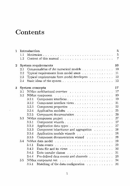
Contents

1 Introduction 51.1 Motivation 51.2 Content of this manual 7

2 System requirements 102.1 Commonalities of the numerical models 102.2 Typical requirements from model users 112.3 Typical requirements from model developers 122.4 Basic ideas of the system 13

3 System concepts 173.1 NiMax architectural overview 173.2 NiMax component 19

3.2.1 Component interfaces 193.2.2 Component interface views 213.2.3 Component properties 223.2.4 Application modules 253.2.5 Component documentation 26

3.3 NiMax component project 273.3.1 Component wizards 273.3.2 Application data types 273.3.3 Component inheritance and aggregation 283.3.4 Application module wizards 283.3.5 Component documentation wizard 28

3.4 NiMax data model 293.4.1 Data events 293.4.2 Data file and its views 303.4.3 Data transfer classes 313.4.4 Pre-defined data events and channels 33

3.5 NiMax component net 343.5.1 Matching of the data configuration 34

3.5.2 Component collaboration 363.5.3 Event-oriented component nets 373.5.4 Component net views 393.5.5 Component aggregation and collaboration 40

3.6 NiMax framework methods 403.6.1 Control methods 413.6.2 Navigation methods 42

3.7 NiMax graphical user interface 43

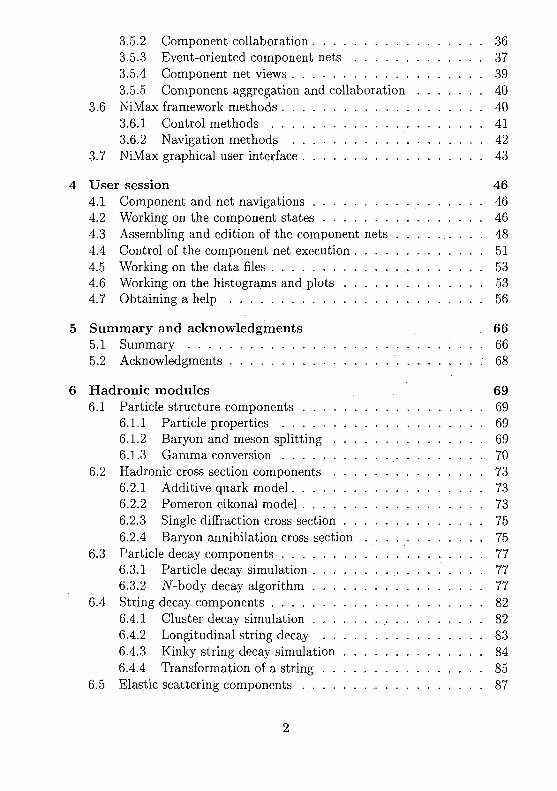
4 User session 464.1 Component and net navigations 464.2 Working on the component states 464.3 Assembling and edition of the component nets 484.4 Control of the component net execution 514.5 Working on the data files 534.6 Working on the histograms and plots 534.7 Obtaining a help 56

5 Summary and acknowledgments 665.1 Summary 665.2 Acknowledgments 68

6 Hadronic modules 696-1 Particle structure components 69

6.1.1 Particle properties 696.1.2 Baryon and meson splitting 696.1.3 Gamma conversion 70

6.2 Hadronic cross section components 736.2.1 Additive quark model 736.2.2 Pomeron eikonal model 736.2.3 Single diffraction cross section 756.2.4 Baryon annihilation cross section 75

6.3 Particle decay components 776.3.1 Particle decay simulation 776.3.2 iV-body decay algorithm 77

6.4 String decay components 826.4.1 Cluster decay simulation 826.4.2 Longitudinal string decay 836.4.3 Kinky string decay simulation 846.4.4 Transformation of a string 85

6.5 Elastic scattering components 87

6.5.1 Hadron elastic scattering 876.5.2 Gluon elastic scattering 886.5.3 Elastic scattering MC procedure 88

6.6 Particle annihilation components 906.6.1 String excitation by a quark annihilation 906.6.2 Quark annihilation weight 906.6.3 Baryon annihilation weight 91

6.7 Particle inelastic collision components 936.7.1 Particle inelastic collision algorithm 936.7.2 Sampling of the longitudinal strings 946.7.3 Sampling of the kinky strings 946.7.4 Longitudinal string excitation 956.7.5 Kinky string excitation 97

6.8 Nuclear model components 1006.8.1 Nuclear properties 1006.8.2 Nucleus initial state simulation 101

6.9 Inelastic nuclear collision components 1046.9.1 Nuclear inelastic collision algorithm 1046.9.2 Initial state simulation 1056.9.3 Nuclear collision participants 106

6.10 Utility components 1106.10.1 Energy-momentum correction 1106.10.2 Particle distributions 110

Chapter 1

Introduction

1.1 Motivation

The full descriptions of relativistic hadronic and nuclear interactions fromthe first principles of quantum chromodynamics (QCD) are very limited. Asa rule we are able to obtain the QCD predictions for the short distance pro-cesses, when interaction takes place with large momentum transfer. However,the processes with the relatively small transferred momenta play a dominantrole in hadronic and nuclear interactions. It is very important task to de-velop and use the QCD motivated models for the predictions, analysis anddescription of these soft processes. Besides, modern experiments related tothe high-energy physics are very complicated and very expensive. The detec-tors design, their construction and their performance require careful numer-ical simulations. This makes Monte Carlo hadronic models to be extremelypopular. As phenomenological models they have many parameters that arefixed by comparison with experimental data. After parameter determinationone can apply the Monte Carlo model to predict the interaction results.

Thus, the MC hadronic models can be used as the hadronic event gen-erators with the main goal to study hadronic collision phenomena as well asthe source of information about hadronic collision final states with the aimto utilize this information [1].

The MC hadronic models are complicated physical models. A typical MCevent generator deals with numerous physical processes. They are based onvery complicated numerical algorithms. Thus, the essential efforts should bedone to formulate, program and test such a model.

There are also different problems faced with the model users in their everyday work on processing experimental data or preparing new experiment. Themost of existing model codes are very difficult in management and commonly

used only by their authors. Even for theorists with good understanding of thehadronic models, it is not easy to apply foreign codes to solve their researchproblems.

An object-oriented approach based on the C++ can be adopted to writethe hadronic MC event generators codes. Such approach has many advan-tages as compared with traditional procedural coding (see, e.g., [2]). Themost important of them are the various facilities of the C++ language todefine new data types along with the operations that are used to manipulatethe types. These are native abstractions (e.g., particle 4-momentum) for MCevent generators domain and we can use them with the flexibility of the built-in data types. We advocate the work on an object-oriented framework [3],since we have observed many commonalities for the hadronic MC models aswell as for their usage and for their development. The framework approachis more justified, when the list of models that chosen for development is verylarge and potentially can be increased.

A typical framework [3] can be considered as well-documented thematiccollection of software to build related applications. It outlines the main ar-chitecture for the application to be developed. The successful frameworkshould not only support needed features and provide default implementationand built-in functionality as much as possible, but it should also allow aneasy modification and extension of the built-in functionality. A goal of anyframework is the reusability. The software developer should be able to reusewritten code, e.g., classes from the framework libraries, and the design of aframework. A framework design is closely connected with the design pat-terns are used to document certain elements of it. A design pattern is theconcise definition of a technique that demonstrates some successful solutionfor particular coding problem. Particularly, the factories and proxies designpatterns (see book [4]) have been applied in our system version.

In this manual we advocate a component approach to the development,assembling and use of numerical models in high-energy physics. The compo-nent can represent a model of either single physical process, e.g., hadronelastic scattering, or very complicated physical phenomenon, e.g., ultra-relativistic heavy-ion collision.

Here we describe a software system that is designed and implementedto support this approach as well as an application of this system for MonteCarlo hadronic event generators. We refer it as the NiMax system. Thecentral system part is an object-oriented framework. We have in mind thatsuch system can be a base to build a library of the model components havingdifferent numerical algorithms. It can allow us to extract model componentsfrom the library pool and compose them into powerful physical models.

We assume that NiMax system will be useful for two categories: the

numerical model users and numerical model developers (advanced users). Weconsider a model user as a person who interacts with the system by means ofa user interface without writing and modifying of the model codes. A modeldeveloper is assumed to work with the system on the level of internal systeminterfaces. A developer needs knowledge of the system concepts, systemstructure and libraries as well as knowledge of C++ language.

In this manual we provide numerous examples of the system user session.We describe also physics and numerical algorithms of the implemented modelcomponents that are included into hadronic modules. These components aredeveloped to perform MC simulations of hadronic and nuclear collisions athigh energies. We would note that this list of components does not exhaust alist of all developed components and components that are under development.Of course, the NiMax system could be applied to find solutions of many othertasks, where the development and use of complicated numerical models isrequired. The chosen list of the MC hadronic components is connected withprofessional activity of the system authors. In our opinion, it is completeenough to demonstrate the most of system features and may help a readerand potential system user to obtain right impression about the system goals.

1.2 Content of this manual

The manual consists of an introduction, three chapters, conclusion and ap-pendix chapter.

In the introduction we stress the importance of problem, explain the sub-ject of work, then we formulate main goals of the work and shortly describethe structure of the manual.

In the first chapter we discuss commonalities of MC hadronic event gen-erators, formulate user and developer requirements for a component-orientedsoftware system. Here we present and shortly discuss basic ideas of thecomponent-oriented NiMax software system.

In the second chapter we present more detailed description of the NiMaxsystem and explain its functionality. At first we give architectural overviewof the main parts of the system and then discuss each part in separate. Wediscuss the component concept. We describe the component interfaces andtheir views. We explain the packaging of components and related softwareinto application domain modules. We consider the development process of anapplication module and component. In particular, we consider applicationdata type classes and some tools for the component development. Here, wediscuss the component documentation. Then we explain the NiMax datamodel concept. We formulate a data event. Then we describe a data file and

7

its views, library of the data transfer classes as well as pre-defined eventsand channels. We provide some details of a component collaboration andexplain the data matching mechanism. Here we formulate the concept ofevent-oriented component nets and describe net's view. At the end of thischapter we present short description of the framework control and navigationmethods.

In the third chapter we describe a user session in more details. Herewe explain how to select a particular component from the list of availablecomponents. We describe the component edition, i.e., an edition of theirinputs, parameters and sub-component substitution. We describe how toreconfigure a component output. Then we discuss how to create a componentnet from several components and edit an existing component net. We explainthe component net execution control. In this chapter we discuss in detailshow to work on a data file, e.g., how to select data. We explain histogramand plot facilities of our system. At the end of the chapter, we discuss howto obtain needed help information.

In the conclusion we give the system and implemented component sum-maries stressing their scientific importance and novelty.

In the appendix chapter we explain physics and numerical algorithmsof the several implemented model components that are included into de-veloped hadronic modules. Some of the implemented components are' sub-components of the implemented composite components. We avoid repeatingdescription of the sub-component physics and algorithms. We would liketo inform an interested reader that physics and numerical algorithms of theimplemented hadronic model components can also be found in the report [1].

Bibliography

[1] Amelin N., Physics and Algorithms of the Hadronic Monte-Carlo EventGenerators. Notes for a developer. CERN/IT/99/6.

[2] Wenaus T. et al., GEANT4: An Object-Oriented Toolkit for Simula-tion in HEP, CERN/LHCC/97-40.

[3] Taligent's Guide: Building Object-Oriented Frameworks, http ://www. ibm.com/java/education/oobuilding /index, html.

[4] Gamma E., Helm R., Johnson R., Vlissides J., Design Patterns. Ele-ments of Reusable Object-Oriented Software, Eddison-Wesley, 1995.

Chapter 2

System requirements

2.1 Commonalities of the numerical models

Even taking a fast look at the MC hadronic models one can see that they havemuch in common [1]. First of all they are phenomenological models havinglarge amount of model parameters. We can specify the parameters as thephysical parameters (hadronic model tuning constants) and hadronic modelconfigurators. The first type of the parameters gives a possibility to changehadronic model results. They operate similarly as a physical input. This typeof parameters fulfils very important job to store physical information abouthadronic processes. The second type of parameters also offers a possibility tochange hadronic model results, but by the changing of an application logicof a numerical algorithm.

Additionally to the parameters much more information should be pro-vided for some hadronic models. For example, the information about phys-ical properties of particles: quark contents, electric charges, masses, decaybranching, etc, is required. The information about physical properties ofstable and excited nuclei: binding energies, spins, level density parameters,fission barrier heights, etc, is also required. Usually such information isneeded in the read-only mode.

The MC hadronic models act in a similar way. They convert an inputdata into an output data answering on the user requests. An input can be thecharacteristics of particles (hadrons, partons, gammas, etc) or characteristicsof nuclei (stable nuclei, excited fragments, etc). An output can be again thecharacteristics of particles or characteristics of nuclei. Acting so any MChadronic model deals with four vectors (energy-momentum, time-position,etc) and their transformations. Any hadronic model somehow handles then-body kinematics.

10

The most of hadronic models are multi-component models. A multi-component model includes other models as additional or alternative modelcomponents and has a complicated execution flow. Especially for the ap-plication purposes a user needs a set of hadronic models to obtain properdescription of the hadronic reaction final states [1].

Practically, all hadronic models are complicated numerical models. Forthem it is not always trivial to separate "physics" from "algorithm", i.e., toseparate physical input, physical parameters, etc influence on the results ofa simulation from a chosen numerical algorithm influence. It is also often,when the same numerical algorithm can be reused within several modelsdescribing of different physical phenomena, e. g., the decay of resonances andexcited nuclei according to the relativistic phase space, the elastic scatteringof partons. hadrons and nuclei, the search collision and decay algorithm forhadron transport model and parton transport model, etc.

Different kind of errors may be occurred during the initialization of ahadronic model or model runtime. The source of errors may be due to theinconsistent user input as well as due to the complexity of numerical algo-rithms. The last situation is often unexpected situation.

Any hadronic model is required to produce different physical outputs,which should be analyzed. An output can be only specific information abouthadronic reaction final states or complete information about the history of agenerated event.

The above list of commonalities can be extended more. For example, be-sides of the kinematics all hadronic MC models deal with random sampling ofdifferent variables according to the different probability distributions, i. e., alarge set of the random number generators is required. Different mathemat-ical utilities: equation solvers, integrators, interpolators, etc, are needed toperform numerical operations. However, it is already clear that the hadronicmodel developers should take into account these commonalities by eithercommon code structure or common used methods or common implementa-tions, etc.

2.2 Typical requirements from model users

The different usage strategies lead to different user requirements for a hadronicmodel package. A user performing theoretical or experimental study ofhadronic collision needs a possibility to play with a chosen model, e.g., thepossibility to visualize and change model parameters, configure the modelor a model component, choose an alternative model component, customizethe model output. Thus, a mechanism to check consistency of the user al-

11

terations should be provided. The run control requires runtime informationand an exception handling mechanism for this type of users.

Another type of users (applied users) is mostly interested in a generatedphysical event itself. The model that is configured for a given type of hadronicreactions with default values of parameters should be offered for the applieduser. The output information should be reduced until required minimum andpresented in the required form.

Of course, the both types of users need to have much more, e.g., a simpleand self-explanatory mechanism for hadronic reaction input preventing fromerrors due to the inconsistent input, analysis and visualization tools are alsorequired to analyze a generated output, etc. Thus, for any kind of users theiruser sessions should be convenient and productive.

2.3 Typical requirements from model devel-opers

Model developers may want to rebuild an existing hadronic model with thegoals to extend a range of its applicability or to increase its predictive power.They may want to incorporate an existing hadronic model for a cooperativework with other existing models. Also they may want to build a new hadronicmodel running standalone or in collaboration with other models.

The enumerated situations are primer tasks of a hadronic model devel-oper that are directly connected with the improvements and extensions ofnumerical algorithms. But in reality he or she should do much more. Forexample, to satisfy user requirements a developer should realize a user inter-face. The interfaces between created hadronic model code and the outsideworld are also needed as well as different adapters, if one wants to use exter-nal packages. A developer should have in mind a possibility for a hadronicpackage to work within another package. A hadronic model developer shouldfacilitate the tasks of future developers as well.

In the conventional approach (see, e.g., [2]) for the developing of thehadronic MC models a developer or several developers are working inde-pendently on a particular model. Such approach, if even an object-orientedlanguage is used, has several drawbacks. First of all, the hadronic modelcommonalities as well as designing and programming experiences are badlyexploited. For example, each new developer has usually started to developa particular hadronic model from scratch. As result of it each new modeldeveloper starts from analysis and design stages. Design duplications aremanpower consuming. The different designs have different qualities and they

12

provide different degrees of satisfaction for the user as well as for the futuremodel developer requirements. The design duplications lead also to duplica-tions in code implementations. The quality of a particular hadronic modelcode depends strongly from the coding experience of a model developer ordevelopers. It is also becomes more difficult to learn, maintain and extend aset of hadronic models created by different developers as well as to connectthem for collaborative work. As a rule the hadronic model developers are notsoftware experts, they are physicists and experts in their subject domains.For them it may be difficult to find a proper solution of the specific softwaretasks.

Thus, as result of the analysis of MC generators and analysis of differentuser and developer requirements it was decided to develop of an object-oriented framework to take into account the hadronic model commonalities,to facilitate user work and to increase the productivity of a developer work.In the frame of a framework the hadronic model users and developers can bemore deeply concentrated on the solution of application domain problems.The developer needs to write much less code since an essential part of theprogram already exists. He or she does not need to be a software expert towrite a robust code. A new model code inherited from the framework couldalso be much easily tested since it is already integrated with the rest of aframework.

2.4 Basic ideas of the system

As it was already discussed the hadronic models as well as their usage andtheir development- have a lot of commonalities. During the system devel-opment we try to separate the observed commonalities from variabilitiesin hadronic model interfaces and their numerical algorithms since commonmeans stable and can be developed only at once.

The central concept of our approach is the concept of a component. Weconsider the model components as unit blocks to construct a composite nu-merical model [3], [4], All such blocks can be stored as an extensible collectionof the model components.

Any model component can be structured into an interface part and thepart presenting its numerical algorithm. The interface part of a model com-ponent allows component interactions with the outside world. By means ofthis part a user can also handle model component parameters and its input-output. We try to formalize the component concept. Such formalizationbecomes visible, when we provide component interface standards. On theother hand the interface standards, if they are required, dictate a model de-

13

veloper to follow definite rules during the component implementation. Theinterface standards facilitate the developing of model component interfacepart, if these rules are taken into account by means of component genera-tion tools. Similar tools we also provide to help the writing of componentdocumentation.

The component developer should mostly work on the implementation ofa particular application algorithm. To facilitate programming of applicationalgorithms for the MC event generators we have developed a library of classesrepresenting physical quantities and many operations on them from a givenapplication domain. We refer these classes as the application data typeclasses. To simplify programming of component input and output we havecreated a library of the data transfer classes.

Object-oriented programmers often use the inheritance mechanism tomodify existing software with minimal efforts. In our case any component isextensible by the inheritance with adding new interface or algorithm func-tions.

Besides of the inheritance mechanism we need another mechanism allow-ing a component developer to use the codes (interfaces and algorithms) ofalready implemented components. Such possibility should not create anyproblem for the component developer to apply C++ programming techniqueduring the implementation of a complicated numerical model or a set ofnumerical models. Such possibility should not create any problem for thecomponent user, e.g., for the access to a sub-component or substitution of asub-component. We offer such mechanism that is referred as the componentaggregation.

A component developer can share some data, functions and classes amongseveral components that belong to a particular application domain or com-ponent category. We have suggested an application module idea for thepackaging of components and component related software. Such module (af-ter its compilation) is loaded in memory as a dynamically linked library.The application modules fulfil twofold function they offer useful software forcomponent developers and hide it from component users.

Either a component or several components can be loaded in memory andeach component is executed as a separate process. A user has a possibil-ity to control execution processes, particularly, due to the different runtimeinformation messages.

Thus, we have defined a component model or formulated a standard com-ponent [3], [4], [5] and suggested several mechanisms of its development andoffered different ways of its management. We have developed a set of classesto support the component development and component management.

Any component deals with data. It may generate very large bulk of the

14

data and store it in a disc. It may read the data from a disc and processit. The collaborative work of several components requires a data exchange.To fulfil these needs we have introduced an idea of the data event [3], [4],[6]. It is a tree-structured portion of data that consists of only values ofthe basic data types. Any data event has its definition that describes eventconfiguration and can be placed directly into memory or stored in a disc. Tosupport data streams we have offered a data file and the component may writeand read data in this file. We have also suggested a mechanism, to controlvirtual data streams. We have suggested a component net concept that isbased on the virtual data streams. The component nets are collections ofdifferent components that are collaborated through their standard interfacesby sending and receiving data event-messages and connected in a sequenceto process numerical data.

Thus, we have defined the data model [6], [7] and developed a set ofclasses, to support data management. The system user has obtained pos-sibilities to configure a component for reliable input and output, navigatethrough stored data, select and visualize data and assemble several compo-nents into a component net.

We try to build a loose system, e.g., by decoupling of objects from theirview objects, by decoupling of different component development, by decou-pling of the file and help sub-systems (see the next chapter).

15

Bibliography



[3] Amelin N. and Komogorov M., An Object-Oriented Framework forthe Hadronic Monte-Carlo Event Generators. JINR Rapid Communi-cations, 1999, No. 5-6 [97]-99, p. 52-84.

[4] Amelin N. and Komogorov M., An Object-Oriented Framework forthe Hadronic Monte-Carlo Event Generators. In Proc. of Int. Conf. onComputing in High Energy and Nuclear Physics (CHEP2000), 7 - 11February 2000, Padova, Italy, p. 119-123.

[5] Komogorov M. and Amelin N., Component-oriented framework forhadron Monte-Carlo event generators. The abstract published in Proc.of XXXIV annual conference of the Finish Physical Society, March9-11, 2000, Espoo, Finland, p. 91.

[6] Amelin N. and Komogorov M., NIMAX: A New Approach to DevelopHadronic Event Generators in HEP. PHYS. P&N LETTERS, 2000,No. 3 [100]-2000, p. 35-47.

[7] Amelin N. and Komogorov M., NIMAX System: A New Approachto Develop, Assemble and Use Numerical Models in HEP. The talkpresented at the XV Int. Seminar on High Energy Physics Problems,Dubna, Russia, 25 - 29 September, 2000; JINR Preprint, El-2001-31,p. 1-14.

16

Chapter 3

System concepts

3.1 NiMax architectural overview

In this chapter we are going to discuss several important parts of the NiMaxsystem that are shown in Fig. 3.1 and their interactions as well.

At the beginning we would like to describe the component concept fromthe software design point of view. Here we will explain different componentproperties that facilitate component management and development.

We will explain the packaging of components that are related to a par-

r Win NT/98 GUI ~1

Framework

ComponentApplication module

Component net

lrs.

Data file

Figure 3.1: NiMax system: an architectural overview.

17

ticular application domain and some software that are shared by these com-ponents into application modules. From the developers point of view thesemodules are parts of component projects that include also the module andcomponent development tools. For system users the modules are preparedas dynamically linked libraries (DLLs).

Then we would like to pay attention for the data management. Particu-larly, we will explain a system data file. In spite of the data file importanceit is only a part of more extended concept that is referred as the data modelconcept. The key point of this concept is the data event.

We will explain the idea of component nets and discuss some details of thenet assembling and execution as well as net peculiarities in the comparisonwith composite component development.

At the end of this chapter we will give short description of the graphicaluser interface (GUI). In the next chapter, where the system user sessions aredescribed, we will provide many more details about the GUI.

We have developed a large set of classes to support component man-agement and development, data management and visualization. This set ofclasses is thought as a framework. Its application programming interface(API), i.e., public or protected methods (open arrows in Fig. 3.1), links to-gether the components, application modules, data files, component nets andGUI.

The NiMax system is written in pure C++ and only the GUI is basedon the Microsoft foundation classes (MFC) library [1]. Only the GUI is anoperational system-dependent part. Now our system with the GUI is workingon different Windows platforms. However, the NiMax system is portable (onthe level of source code), if it is applied in the command line mode.

We would note that we apply a document - view technology (see [1])within our system. The main idea of this technology is a separation of doc-ument objects that hold data from the objects that display data and allowediting. The views show different facets (or several the same facets) of thesame data and, e.g., if a user edits an active view, then all other views mustbe updated. Each document (component, component net, etc) is connectedwith a file having unique extension. This technology allows a development ofdifferent visualization and edition systems without changing of a data controlsystem.

The recent version of the NiMax system includes four types of documents.The first type is referred as a workspace. The main information that is keptin the workspace document is a list of registered components. The secondtype is a component net file. It holds information about component states(parameter values, data output configurations, description of component re-lations, etc). The third type is a data file. The fourth type is a file for thestorage of graphical information.

18

The document - view technology allows independent extensions of num-bers of document's types and their views. For example, we have developeda help system that uses html documents. These documents can be browsedand edited by some standard tools that belong to an operational system.Our help system could be used separately from the NiMax system for adver-tisement and for studying of the implemented model components.

3.2 NiMax componentIn this section we are going to discuss the component interfaces and theirviews. Then we explain different properties of the components. The compo-nent packaging is an important issue for component development and man-agement will also be described. Finally, we shall discuss the componentdocumentation.

3.2.1 Component interfaces

We can consider any component as a set of standardized interfaces. By meansof the interfaces the component client (user, framework or another compo-nent) can talk with the component asking a definite service. Only throughinterfaces a component communicates with the outside world. An interfaceincludes several methods and some related data. Let us explain functionalityof the standardized NiMax component interfaces that are presented in Figs.3.2 - 3.3.

By means of the input interface a user sends a request for a componentand provides necessary input data to fulfill this request. The request as well

Input . , Outputinterface interface

Tuninginterface

Figure 3.2: Main component interfaces.

19

as input data is provided in a form of an input map [2], [3]. The input map isa list of simple data types and has linear structure of data. We can refer inputmaps as user-friendly linearly structured data. If the component may startto run from a request obtained by its input interface the system considerssuch component as a main component.

The tuning interface gives a possibility to tune a component with aim toobtain reliable result from its execution. By means of this interface a userhas access for model parameters and switches. The framework includes aset of classes to support the parameter and input map management [2]. Wewould note that the input interface and tuning interface have many similar-ities from the developer's point of view (the same classes in use, the samedata structures in use). An input map data can be understood as a list ofmandatory parameters that must be specified by users before the componentexecution.

The result of a component execution (output data) is obtained by meansof the output interface. This interface assists either to write the componentoutput data in a data file or to send the component output data for othercomponents. The output data are produced as configured data events andhave a tree structure [4], [5] in the common case (see the next section formore details).

A component can also read its input from a data file or receive it fromother components. In these cases it starts to run from a request obtained bythe matching interface. The matching interface allows for the component toselect data from an input data flow according to a matching configuration [4],[5]. A particular matching configuration is realized as a matching map. Thematching maps are different from the input maps. They do not include dataand include only data configurations (see the next section for more details).

Matching Outputinterface interface

Tuninginterface

Figure 3.3: Component interfaces.

20

The component user is not able to change these configurations, but he or shecan enable or disable a particular matching map for a chosen component.We can refer the matching maps as developer-defined data configurations.

We have also developed a runtime information interface (it is not shownin Figs. 3.2 - 3.3). It is used to obtain and control component runtimemessages (see the NiMax framework methods section for more details).

Besides of the outlined standard interfaces each particular component hasits API, i.e., a set of public and protected methods, which implements thecomponent functionality and can be called directly or indirectly by means ofthe component standard interface methods.

We can classify different types of the components according to a presenceor absence of a particular interface or interfaces. For example, we distin-guish runnable components that have input interfaces or matching interfacesfrom general components that have neither input nor matching interfacesand cannot be executed, but they are useful as sub-components.

The system allows an extension of existing interfaces as well as adding ofnew ones. We can imagine a component that needs an external data interfaceto receive the data having external format. For example, a component canneed an additional standard interface to manage data from a database. Thus,by adding more standard component interfaces we can extend an applicationarea of the NiMax system and facilitate the work of a component developerin this application area.

3.2.2 Component interface views

Each component interface is complemented by at least one view as it isshown in Fig. 3.4. To obtain the component interface views the componentobjects should be created (see below). These views allow a visualization of thecomponent input maps, component matching maps, component parameters,its output configuration, a structure of a composite component as well ascomponent runtime information. These views help the component user toperform many actions on the component state (see the next chapter). Acomponent interface can be connected with several views to realize differentways of its data display and edition, but each view object is related to onlyone interface. It is important to stress that changing of a view or adding of anew view does not require a changing of its interface. It allows an independent(from rest of the system) improvement and extension of the graphical userinterface. Besides the component interface views there are more views thatpertain a component, e.g., the component documentation view that helps auser to learn this component.

21

3.2.3 Component properties

Besides of the standardized interfaces and views, the system componentshave other common elements (see Fig. 3.5). Each component has its owncomponent factory [6] to create the component objects. By means of thecomponent factory one can obtain static information about the component.The term static points out that there are no created component objects. Thisinformation is either used for a component object creation [6] or to navigatethrough a component list. On the contrary dynamic information such as alist of component parameter values, its input and output data configurations,etc, requires that component objects should be created.

The main element of the component static information is its unique identi-fier [7]. Knowledge of a component's identifier helps us to obtain full informa-tion about the component. The attachment of unique component identifiersallows us to develop a simple and efficient component control mechanism.Particularly, a composite component that is aggregating (see below) othercomponents should include their proxies [6], which have the component iden-tifiers as proxy's members.

Fig. 3.6 demonstrates an existence of the component inheritance that issupported by the NiMax system. From any component one can derive a newcomponent. Thus, we distinguish base and derived components. Standardinterfaces of a base component and derived component are joined as well astheir public APIs (see Fig. 3.6).

Outputconfiguration

view

Figure 3.4: Component interface views.

22

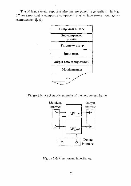
The NiMax system supports also the component aggregation. In Fig.3.7 we show that a composite component may include several aggregatedcomponents [4], [5].

Component factory

Sub-componentproxies

Parameter group

Input maps

Output data configurations

Matching maps

Figure 3.5: A schematic example of the component frame.

Matchinginterface

Outputinterface

Tuninginterface

Figure 3.6: Component inheritance.

23

We would note that these components could belong to the different DLLs.An aggregated component may aggregate other aggregated components. Aparticular component may include a tree of the aggregated components orsub-components. The tuning and output interfaces of an aggregated compo-nent are simply joined to the relevant aggregating component interfaces (seeFig. 3.7).

We would stress several important features of the suggested aggregationmechanism. A component user is able to see a composite component struc-ture and has access to any sub-components by means of the GUI.

The inheritance and aggregation mechanisms provide a unique possibility

Inputinterface

C1

ci)

c?

c

API_r

ii

Outputinterface

l > !4>!Tuning

interface

Figure 3.7: Component aggregation.

C1

c

C 2

) C

Figure 3.8: Sub-component substitution.

24

for the composite component users to change component algorithms withouttouching of the component source codes and their recompilations. We referthis possibility as the runtime substitution of sub-components in compositecomponents (see Fig. 3.8).

3.2.4 Application modules

Several implemented components may share common functions and classesas well as common data that are related to a particular application domain.The development of a component related software that does not belong toparticular components facilitates the work of component developers and in-creases developer's productivity. Such development is also argued by moreefficient use of computer resources and gives a possibility to create scalablesystem from independent blocks.

We suggest packaging of built components with some related softwareinto modules. We refer these modules as the application modules due to therelation of their content with application domains. For example, they canbe the hadronic model modules (see below) or modules to predict electro-magnetic processes or modules to describe a low-energy neutron transport infissile media, etc. An example of the module content is presented in Fig. 3.9.Besides of the components, application data types (see the next section) and

Components

Application data types

Data transfer classes

Tables

Units and constants

Figure 3.9: An example of the application module content.

25

data transfer classes [2] are members of the application modules. It is impor-tant to stress that application modules hide all software from the componentusers excepting the components.

The application modules can be self-sufficient on the level of source codes,i.e., no external methods, no external implementations, etc, are required tocompile and execute the module components. It allows us to use these mod-ules as distribution or exchange units. However, the module independencedoes not forbid use of components from other modules. It does not pose a lim-itation for the inheritance and aggregation mechanism. For example, it doesnot forbid the sub-component substitution in the case, when an aggregatingcomponent and some alternative component belong to different dynamicallylinked libraries (compiled modules). Thus, the application modules can ei-ther be completely independent from each other or they connected with othermodules for some applications. In the last case they include lists of requiredmodule references.

A large set of hadronic model components have been already implementedand included into hadronic model modules (see the hadronic modules chap-ter).

The MeV, GeV, barn, Plank constant and other units and constants areincluded into the hadronic model modules. We have adopted a convenientstrategy to use the physical units and physical constants from the GEANT4toolkit [8].

Physical tables that store information about physical properties of parti-cles and nuclei may be parts of the modules. Table information is requestedin read-only mode. This fact opens a possibility to handle the tables byexternal tools, e.g., by external databases. We have already created severaldatabase tables containing particle and nuclear properties. Each of thesetables can be visualized, edited, extended, etc, separately by the Microsoftdatabase tools. We are working on a standard Structured Query Language(SQL) interface for the components to provide their access to data tablesstored as database files.

We have included many special and utility functions and classes, e.g.,3 and 4-vectors, random number generators, sorting methods, etc, into thehadronic modules. A large number of such classes are borrowed from theCLHEP library [3].

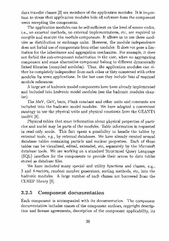
3.2.5 Component documentationEach component is accompanied with its documentation. The componentdocumentation includes names of the component authors, copyright descrip-tion and license agreements, description of the component applicability, its

26

input maps, parameters, matching maps, output configurations, component'sAPI, sub-components in use, etc. The component documentation is realizedas a set of HTML files.

3.3 NiMax component project

In this section we are going to discuss several mechanisms and tools for thecomponent development as well as application data types. They are differentparts of a component development concept referred as the component project.Within a component project the component developers are also able to usedata transfer classes (see the data model section).

3.3.1 Component wizards

The observation of many common component elements allow us to developcomponent frames (see Fig. 3.5) [2], [3] with the aim to produce the so-calledskeleton components simply by editing of the particular component frame.Such frame can be thought as a component template that is supporting acorrect programming style. Thus, a component developer needs to designonly a component application algorithm. To help component developers wehave designed component wizards that are similar to the Microsoft VisualC++ 6.0 class wizard [1]. A component wizard is a code generator thatproduces a component skeleton by means of the use of dialog windows. Theresult of its work is a set of correctly related files with classes and interfaces.

3.3.2 Application data types

With the aims to increase a productivity of hadronic component developersand provide a robustness of the component algorithms we have created anapplication data types (ADT) library of classes. The library was developedto represent key abstractions (application domain data types) and opera-tions that are used to manipulate the types. The development of MC eventgenerators is our problem domain. Thus, the most of the ADT objects arecounterparts of real high-energy physics objects (particle, parton, nucleus,string, etc).

We are extending our ADT library to help algorithm developers in theirwork on the hadronic model components and on components for simulation ofelectromagnetic processes of particle and nuclear interactions at wide energyrange. Our goal is to implement a large set of the ADT classes allowing analgorithm development for a simulation of the particle and nucleus transport

27

through composite media. We plan that new ADT libraries will includealready mentioned classes for a description of particles and nuclei, classesfor a description of particle transport, the so-called tracers, classes for adescription of materials and geometry of the media.

3.3.3 Component inheritance and aggregation

As we already said a component developer can extend the functionality ofan existing component by applying of the component inheritance mechanism(see Fig. 3.6) that is supported by the NiMax system. For example, thecomponent inheritance is a convenient way to add either new input maps ornew matching maps. A new component can be developed by the aggregationof existing components [4], [5] (see Fig. 3.7). There are no limitations forcomponent developers to create a large and efficient component code as com-pared with the standard C++ coding, if they are applying the componentaggregation. In this case the component coding is even more simplified. Forexample, no efforts are required to create and destroy sub-component ob-jects. The framework fulfills a control of the sub-component objects (see theNiMax framework methods section). Thus, C++ programmers can use thecomponents as usual C++ classes excepting of component object creationand destroy.

3.3.4 Application module wizards

As we already explained built components are packed with some relatedsoftware into the application domain modules. We consider the applicationmodules as development's units. For a component developer it is more natu-ral and more efficient to work on a component code within some componentrelated software environment than on an isolated component code. The workon isolated codes leads to code and data duplications.

To support an implementation of the module structures we have devel-oped application module frames. We are working on application modulegenerators (wizards) for component developers and a module navigator forcomponent users that is allowing of the use of the graphical user interface.

3.3.5 Component documentation wizard

The writing of component documentation is very important part of the com-ponent development process. We have developed documentation frames anddocumentation wizards (for the Windows platform only) for component devel-opers. These tools help the developer to prepare and present information for

28

a standard appearance. The documentation frames are different for differenttypes of model components. They are similar to the component frames dis-cussed below and developed in a complement of the model component frames.The documentation wizards scan source codes of the application modules (orseparate components) and generate initial versions of documentation files.These files could be further edited and extended by the developer by meansof dialog windows coming one by one. After the developer has passed allsteps, it is possible to run the Windows HTML Help compiler with the aimto create help topics files for a search of the necessary information by key-words or contents. Obtained files are integrated into the help sub-system.

3.4 NiMax data model

In this section we are going to consider different mechanisms of the dataexchange, data storage, data visualization and data processing that are sup-ported by the NiMax system. Here we shall also introduce the main conceptsthat are used to describe the NiMax data model such as the data event, datafile and its views, pre-defined events and pre-defined channels and data trans-fer classes.

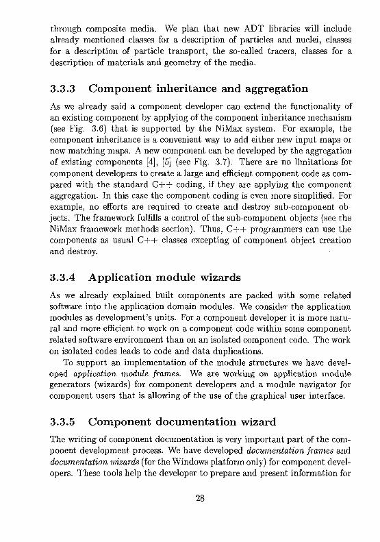
3.4.1 Data eventsThe data event [4], [5] is an elementary data unit for the data exchange. Itis a portion of data that consists only of values of the simple data types (int,float, double, etc). Any data event has its definition. The definition includesa unique identifier (sometimes we refer it as a data event type) and describesa data event configuration. The data event configuration is a set of datachannel definitions. The data channel definition includes a channel identifier,channel type, channel name and more information can be added. We wouldstress that the data channel is an elementary unit for data processing in theNiMax system, since the most of the data operations can be fulfilled on aseparate channel. An example of the data event configuration is shown inFig. 3.10 in a comparison with C-structures. Any data event configurationis bounded by external brackets. Inside of the external brackets there canbe separate channels, arrays of channels and groups of channels boundedby inner brackets. The array of channels has a special flag in the channeldefinition and the information about size of the array that is written in thechannel data part. Inside of the internal brackets there can be again separatechannels, arrays of channels and the group of channels bounded by the innerbrackets and so on. Thus, each data event configuration can include a tree

29

of channel definitions. The basic or simple data types can be grouped insideof the data event to represent more complicated data structures, e.g., torepresent C arrays, C structures as well as C array of arrays and array ofstructures (see Fig. 3.10). We would note that the data event is not a C++object, i.e., it is not an instance of the definite class.

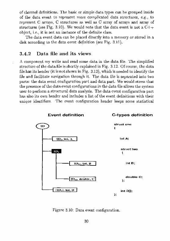
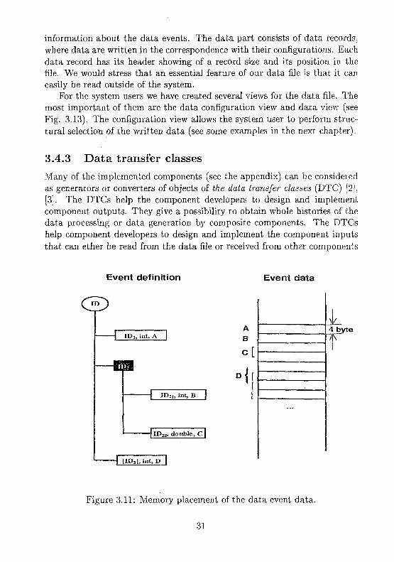
The data event data can be placed directly into a memory or stored in adisk according to the data event definition (see Fig. 3.11).

3.4.2 Data file and its viewsA component my write and read some data in the data file. The simplifiedstructure of the data file is shortly explained in Fig. 3.12. Of course, the datafile has its header (it is not shown in Fig. 3.12), which is needed to identify thefile and facilitate navigation through it. The data file is separated into twoparts: the data event configuration part and data part. We would stress thatthe presence of the data event configurations in the data file allows the systemuser to perform a structural data analysis. The data event configuration parthas also its own header and includes a list of the event definitions with theirunique identifiers. The event configuration header keeps some statistical

Event definition C-types definition

IDi, Int, A I

ID21, Int, B

IID22, double , C |

, Int, D |

struct one

int A;

struct two

int B;

double C;

int DO;

Figure 3.10: Data event configuration.

30

information about the data events. The data part consists of data records,where data are written in the correspondence with their configurations. Eachdata record has its header showing of a record size and its position in thefile. We would stress that an essential feature of our data file is that it caneasily be read outside of the system.

For the system users we have created several views for the data file. Themost important of them are the data configuration view and data view (seeFig. 3.13). The configuration view allows the system user to perform struc-tural selection of the written data (see some examples in the next chapter).

3.4.3 Data transfer classes

Many of the implemented components (see the appendix) can be consideredas generators or converters of objects of the data transfer classes (DTC) [2],[3]. The DTCs help the component developers to design and implementcomponent outputs. They give a possibility to obtain whole histories of thedata processing or data generation by composite components. The DTCshelp component developers to design and implement the component inputsthat can ether be read from the data file or received from other components

Event definition Event data

IDi, int, A IA

B

c[

ID21, int, B j

flD2z, double, CI

P3] , int, D |

4byte

t

Figure 3.11: Memory placement of the data event data.

31

(see the component net section). Thus, the DTC library allows componentdevelopers to pay more attention for the development of component algo-rithms, because the developer does not need to think about details of theinput-output operations. The DTCs help component developers to designand implement universal numerical algorithms. A degree of the universality

Eventheader

IS Event1 data

Figure 3.12: Data file structure.

Dataconfiguration

view

Figure 3.13: Data file views.

32

of an algorithm is determined by the amount of needed input-output infor-mation. Our DTC library has a hierarchical structure. The most universalalgorithms are those that use, as an input and output, the objects of nodedata transfer classes.

We would note that data transport classes are essentially the same as theapplication data types classes, which were discussed before. By introducing ofthe data transfer term for a set of classes we would stress their importance forthe data exchange. Beside of the implementation of MC model componentsit is necessary to develop similar sets of classes in other application domains.Within our system we have no strict recommendations how to build suchclasses. The most important thing is that any object of the application datatype class should support a serialization in the sense that it needs methods towrite to the data file and read from the data file (see the NiMax data modelsection) its object states. Taking into account this fact we have created datatransfer class frames (they are similar as the component frames mentionedabove) with the aim to help the component developers.

3.4.4 Pre-defined data events and channelsWe have suggested [4], [5] a concept of the pre-defined data events and chan-nels within our system. These events and channels are associated with def-inite services that are offered for the system users. The main idea of thisconcept is to increase a productivity of the system users that belong to par-ticular application domains. This concept allows an independent extension ofsystem service facilities, e.g., to create user interfaces adapted to particularapplications. For example, in the high-energy physics domain the users oftenuse histograms. The contents of one- and two-dimensional histograms andtwo-dimensional plots can be written, read and visualized as the pre-definedgroups of channels as it is shown in Fig. 3.13 (see some histogram and plotexamples in the next chapter). To deal with such data events and channelsthe framework needs to know only their identifiers. Thus, the frameworkknows (due to the unique identifiers) how to display table and graphicalviews for the pre-defined histogram and plot channels The component pa-rameters, input maps and proxy sets are other examples of the pre-definedevents representing component states. Again, the framework knows how todisplay and execute such data events.

We would mention that the pre-defined channels and pre-defined group ofchannels have fixed configurations (similarity with C++ objects) and theiridentificators can be considered as their types. The system user is not ableto change their configurations.

33

3.5 NiMax component net

In this section we are going to discuss the interaction between components,when components exchange their data. They exchange data by means ofthe data file or through the virtual data stream. In the second case someof the interacting components are joined into a component net and a directdata exchange takes place. Before to describe the component net concept wewould like to explain how a component is able to select needed input datafrom the data produced by another component.

3.5.1 Matching of the data configurationThe idea of an input data selection for a component from the data producedby another component [4], [5] is illustrated by the Figs. 3.15 - 3.16. Produceddata events have linear or tree structures. They are described by their eventconfigurations as it was explained above. The framework analyses eventconfigurations and searches a necessary sub-configuration for a component.We refer this process as the matching of a data configuration. The necessarydata configurations for a given component are described by the componentmatching configurations or matching maps. If the necessary configurationis found we refer this situation as an observation of an entry point into thedata described by the configuration.

There are some peculiarities, when a component receives a data eventproduced by another component. It either takes a part of the event data

One-dimensionalhistogram

views

Figure 3.14: Pre-defined data event views.

34

according to its matching configuration or it absorbs the whole event data,where such matching configuration was found. We consider components withthe second type of their behaviors as data event filters. The filtered dataevents can be modified as well.

The component developers may offer several matching maps. Thus, thereis a room for the component users to tune such component with the aimto recognize an event channel or several channels from sent or read dataevents that it expects to receive. Any of the matching configurations can beregistered as a default one. It can be a situation, when the framework willfind several suitable (according to a matching map) sub-configurations in theanalyzed data event and several entry points into the data are obtained. Itis another room for the component users that is connected with a choice ofan entry point.

It is important to stress that working on a particular component im-plementation component developers do not need to learn or use system orcomponent classes (objects) with the aim to support a component collabo-ration [4]. The component developers do not need to learn configurationsof the data events that can be received by a component. The componentdevelopers are not required to have knowledge about the source (the datafile, other components) of events that the component will receive. He or shehas to know how to write configurations of the required input data.

Kvent dataconfiguration

Matching dataconfiguration

Selected dataconfiguration

Figure 3.15: Selection of the linearly structured data.

35

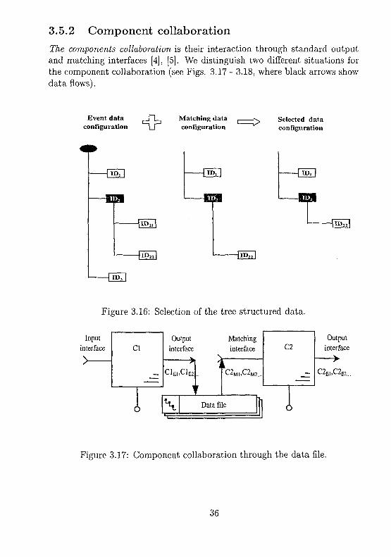
3.5.2 Component collaborationThe components collaboration is their interaction through standard outputand matching interfaces [4], [5]. We distinguish two different situations forthe component collaboration (see Figs. 3.17 - 3.18, where black arrows showdata flows).

Event data flconfiguration ^

Matching dataconfiguration

Selected dataconfiguration

-ESS

Figure 3.16: Selection of the tree structured data.

Inputinterface Cl

1

Outputinterface

CIEI

\

— ^

C1E2

\1

t

Matchinginterface

i

C2 M ] ,C2 M 2

Data file 11

a.

i

Outputinterface

Figure 3.17: Component collaboration through the data file.

36

The first one is that a component writes its output in a data file andanother component reads data from the data file for further processing. Wedemonstrate the first situation in Fig. 3.17. In the figure a component Clproduces many data events having different configurations: CIEU C1B2, etc,and writes these events in a data file. A component C2 reads the data fileand selects data according to matching configurations: C2MI, C2M2, etc.We consider the shown situation as the component collaboration through adata file bus having in mind a hardware analogy. For this type of interactioncomponent objects are completely isolated from each other.

We would stress that a reading component does not need to wait for whena writing component finishes to write all events. It can start to read dataevents immediately after the first event has been written. This feature isparticularly important for a data monitoring.

The second situation (see Fig. 3.18) is that one component produces adata event output, which will be received by another component as an input.We consider this situation as the component collaboration by a data eventbus. For this type of interaction several components are executed inside acommon process.

3.5.3 Event-oriented component netsA set of components that collaborates through the standard output and match-ing interfaces by sending and receiving data event messages is referred as an

Cl

- —'

1"-'V,

Clm C2MI

>,C2

1C3

I >\

C3Hf \

C2E,

f

- 4Figure 3.18: Event-oriented component net.

37

event-oriented component net [4], [5]. Fig. 3.18 demonstrates an exampleof a net. Here, a component C\ produces two events having configurations:Clsi and C\E2, then components C2 and C3 receive some selected data ofthese events. The data are selected in the accordance with matching config-urations C2Mi and C3MI, respectively. The components C2 and C3 producenew data events that are configured as C2EI and C3EI, respectively. Thelast events are written in a data file.

There is a direct hardware analogy of the described component net ex-ample and the matching mechanism of input data selection that is presentedin Fig. 3.19. In this figure different lines denote different wires that maylink components. Several wires can be screwed into a cable. A cable caninclude sub-cables ("tree structure" of a cable) as well. The wire analogy isa data event channel (simple data type) and the cable analogy is a group ofchannels or a data event configuration. The analogy of a data configurationmatching is that only some wires or sub-cables from an outgoing cable arechosen for component connections.

Following the hardware analogy we would like to provide more detailsabout component connections. Inside the output and matching interfaceswe can distinguish groups of methods that are referred by us as the outputand matching connectors. A component processes data through a connec-tor. Components can be wired through the connectors. Any connector dealswith two important things: a data stream (a data file, memory) and data

Figure 3.19: Hardware analogy of the event-oriented component net.

38

event configuration (an output configuration, matching configuration). Theconnector concept allows the component users to redirect and reconfigurecomponent output and input data. The user can choose a particular streamor tune a particular output configuration or choose a particular matchingmap (see some examples in the next chapter).

We would note that a sub-component of an aggregating component can-not be linked with some components or a data file through its matchingconnector. All components in a component net deal with only one data file.

We consider only the nets, those component execution orders are definedby data flows, i.e., we consider only pipeline nets. Thus, any net includesthe component that is executed at first. We refer this component as thestart or main component (it expects to receive the so-called start event).It reads its input by the input or matching interface. We should note thatany component or sub-component from a net is able to write its output to adata file. So far each component can have only one input connector and oneoutput connector and such components could be linked only into "linear"pipeline nets.

Any event-oriented net needs an event control procedure should be writ-ten besides the information about component connections. But, for pipelinenets, such procedure can be written and compiled at once and hidden fromthe system users.

3.5.4 Component net views

Any net is a NiMax system file that consists of two parts. As any file itcan be saved for later re-use, re-named, deleted, etc. The first part canbe considered as the net definition part. The second part includes a dataevent control procedure. This first part is constructed by the framework onthe basis of the information obtained from a user through the net views.The framework generates the second part by itself. The net definition partincludes the information about pairs of collaborated components. It notifiesalso a start component and end-net components. Providing such informationone assembles a net through the net views. By the net views one can selectany net component and show its structure, parameters, output configurationand matching maps as well as input maps for a main component of the net(see the net editor examples). Very often a net includes only one component.Thus, performing a component execution, we always deal with a net file. Anycomponent, which can be a net member, is referred as a runnable component.

39

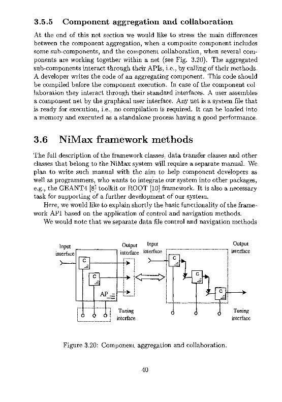
3.5.5 Component aggregation and collaboration

At the end of this net section we would like to stress the main differencesbetween the component aggregation, when a composite component includessome sub-components, and the component collaboration, when several com-ponents are working together within a net (see Fig. 3.20). The aggregatedsub-components interact through their APIs, i.e., by calling of their methods.A developer writes the code of an aggregating component. This code shouldbe compiled before the component execution. In case of the component col-laboration they interact through their standard interfaces. A user assemblesa component net by the graphical user interface. Any net is a system file thatis ready for execution, i.e., no compilation is required. It can be loaded intoa memory and executed as a standalone process having a good performance.

3.6 NiMax framework methods

The full description of the framework classes, data transfer classes and otherclasses that belong to the NiMax system will require a separate manual. Weplan to write such manual with the aim to help component developers aswell as programmers, who wants to integrate our system into other packages,e.g., the GEANT4 [8] toolkit or ROOT [10] framework. It is also a necessarytask for supporting of a further development of our system.

Here, we would like to explain shortly the basic functionality of the frame-work API based on the application of control and navigation methods.

We would note that we separate data file control and navigation methods

Inputinterface

Outputinterface interface

Outputinterface

Tuninginterface

Figure 3.20: Component aggregation and collaboration.

40

from the rest framework methods. Such separation makes sense, because thedata file, data file views and data file control and navigation methods arejoined into an independent data file system having its own applications.

Before to start the description of the control and navigation methodswe would like to say a few words about object identifiers. Any object of oursystem has its unique identifier as well as any data event discussed above. Theknowledge of an object's identifier offers full information about the object.At the moment for identifier's values we use integer numbers (unsigned type).Thus, we have a possibility to assign more than 4 billion different values. Theinteger numbers are very convenient for searching and navigation.

3.6.1 Control methods

There are many methods to control the component life cycle, i.e., a compo-nent instance creation phase, edition phase, execution phase and destructionphase.

In spite of the fact that the component life cycle consists mostly of internalframework processes, which are hidden from the framework users we wouldlike to give an idea about it. There are many possibilities for the user toinfluence the component life cycle.

Before to start an object creation procedure the framework creates anenvironment for the component object. The content of this environmentdefines creation mode, optional variables, which are set to default values,and output and input files, if they will be used. The users are able to modifydefault values of these optional variables by means of the user interface, e.g., the users can either set their own default parameters and input mapor suppress some data event output or suppress some runtime informationoutput, etc.

There are two special modes of any component (excepting the virtualone) for an instance creation. The first special mode is the instance creationfor only information purpose. This means that the user cannot make anychanges of a component object. This mode provides a possibility for theuser to learn the component structure by the user interface. The secondspecial mode is the debug mode. It gives a possibility of creating a generalcomponent instance without the permission to execute it. This mode is addedin order to debug the component interfaces.

In the case of a composite component, the aggregating component in-stance is created at first. Then the framework will create its aggregatedcomponent or sub-component instances. The order of the aggregated in-stance creation follows their definition order in the aggregating component.In order to create any component object the framework needs to know only

41

the component's identifier. It uses sub-component's identifiers to look fortheir factories. If a factory is not found, the framework tries to find an al-ternative sub-component according to the component proxy definitions andcomponent inheritance hierarchy. The user is able to control this process byan enabling or disabling of a component substitution. The creation processis repeated for each sub-component component and for their sub-componentsuntil all component objects will be created.

The destruction phase for created component objects is fulfilled in a re-verse order as compared to the construction phase without the user influence.

During the component edition phase the user is able to edit parame-ters and input or matching maps as well as reconfigure component's output.Check methods are called to control a consistency of the edition. In the caseof a non-consistency these methods send warning messages and set back tothe default values the values of edited variables.

The framework helps the system users to create, edit and execute net filesand controls these processes. During the execution phase the framework sup-ports component runtime information output: information messages, warn-ing messages and error messages (see some examples in the next chapter). Inthe case of warning or error messages help information (see below) is offeredfor the interested user.

The framework allows the user to execute several component nets as sep-arate processes and control their executions. In the case of an error theframework detects itself a place of the error and the component developersdo not need to make some special efforts to solve this task.

3.6.2 Navigation methods

The framework fulfills component librarian functions. It allows the user tovisualize a total list of the components are included into the system andregister a required component. Before a component registration the compo-nent views show static information, because the component objects are notcreated yet. The component registration means the creation of componentobjects. The framework allows the user to look through net files, open themfor net editions and save the edited nets.

Tree structures are heavily used in our system, e.g., the tree structure ofcomposite components and tree structure of data events. Thus, the methodsto navigate through a composite component and through a data file are thesame.

Here we would like to mention that using file navigation methods themodel developers are also able to write adapter or driver tools to transform

42

the format of a data written down to the system data file into data formats,which are acceptable for the external packages.

Besides of runtime information and different information messages, whichcan appear during a component life cycle, the system users are offered moredetailed help information. The users can navigate through the help docu-mentation either by contents or by keywords.

As we already said any object in our system such as a component, pa-rameter, error message, etc, has a unique identifier. It opens a possibility tobind these identifiers with HTML files that are describing the objects. Thus,the users may obtain a help from the "inside" of a code by means of a uniqueidentifier, e.g., by a parameter identifier the framework opens the HTML filethat describes the parameter.

3.7 NiMax graphical user interface

The NiMax GUI is developed in the accordance with the document - viewtechnology [3] that was shortly discussed at the beginning of this chapter.This technology is very suitable to take into account the system user require-ments.

After starting of the NiMax system, the main window will appear. Thiswindow includes many views. These views can be thought as different navi-gators and editors. All available components are displayed for system users.The system user can launch any component and open any available compo-nent net file for a further edition. By means of the component editor the usercan edit input maps, parameters and substitute sub-components. We wouldstress that the system user sees the whole structure of a composite componentand can edit and perform substitution of any sub-components of this compo-nent. The user can reconfigure the component and sub-component outputs.By the net editor the user can assemble several components into a componentnet and modify an existing net. The system user can perform controlled exe-cutions of several nets as separate processes. The user can navigate througha data event configuration and data event data in a data file performing thestructural data selection. The user can visualize the data produced by com-ponents as one-dimensional histograms and two-dimensional histograms andplots. The user can navigate through the help documentation looking fornecessary information about a particular component or the NiMax systemitself.

43

Bibliography

[1] Kruglinski D. J., Shepherd G., Wingo S. - Programming MicrosoftVisual C++ , Fifth Edition, Microsoft Press, 1998.

[2] Amelin N. and Komogorov M., An Object-Oriented Framework forthe Hadronic Monte-Carlo Event Generators. JINR Rapid Communi-cations, 1999, No. 5-6 [97]-99, p. 52-84.

[3] Amelin N. and Komogorov M., An Object-Oriented Framework forthe Hadronic Monte-Carlo Event Generators. In Proc. of Int. Conf. onComputing in High Energy and Nuclear Physics (CHEP2000), 7 - 1 1February 2000, Padova, Italy, p. 119-123.


[5] Amelin N. and Komogorov M., NIMAX System: A New Approachto Develop, Assemble and Use Numerical Models in HEP. The talkpresented at the XV Int. Seminar on High Energy Physics Problems,Dubna, Russia, 25 - 29 September, 2000 (will be published in Proceed-ing); JINR Preprint, El-2001-31, p. 1-14.

[6] Gamma E., Helm R., Johnson R., Vlissides J., Design Patterns. Ele-ments of Reusable Object-Oriented Software, Eddison-Wesley, 1995.

[7] Orfali R., Harkey D., Edwards J., The essential distributed objects.Survival guide., John Wiley and Sons, Inc., 1996.

44


[9] Class Library for High Energy Physics,http : I /wwwcl.cern.ch/asd/lhc + +/cl hep /index, html

[10] Brun R. et al, ROOT System, CERN/HP, 1997. See http ://root.cern.ch/.

45

Chapter 4

User session

4.1 Component and net navigations

The available model components and component nets are displayed for thesystem users. There are three different possibilities to look through thetotal component list (see Fig. 4.1): by categories (default view) to showthe components from different application categories, by modules (DLLs) toshow the DLL component contents, by hierarchies to show the componentinheritance relations. The component views show also the component typesthat are defined by a presence or absence of particular standard interfaces[1]. The icons mark the component types: runnable components, generalcomponents, virtual components, etc). The file browser fulfills the functionof a net navigator. It offers access to component nets by the open commandfrom the file menu. The net user can also rename, copy and delete the netfiles.

4.2 Working on the component states

The framework offers for the component users a possibility to change a com-ponent state (see Figs. 4.2 - 4.3) by means of the component interface views.The user can see, register (instead of a default input map) and edit compo-nent input maps as well as see and edit component parameters. The frame-work checks an inconsistency of the parameter edition (see, e.g., the warningmessage in the bottom of Fig. 4.2). During input map and parameter edi-tions the user always has a possibility to set back their default values. Theuser has also access to any parameter of a sub-component inside a compositecomponent (see Fig. 4.3).

A sub-component can be substituted by another sub-component, if they

46

have a common base component. To see that components have a commonbase component the user can use the component hierarchy view. Thus, insidethe composite component an aggregated component can be substituted byan alternative component without coding, i.e., by means of the user interfaceas it is shown in Fig. 4.4. The component user can perform substitutioninside any sub-component, if it is a composite one. It is a way to change andupdate the application algorithms of composite components.

If a component is expected to produce an output, the component user hasa possibility to control it. The total events or only some selected channelscan be disabled for the output. In the case of composite components, theoutput reconfiguration can be performed for any sub-components (see Fig.4.5).

If a component is expected to receive data either from another componentor from a data file, the component user has a possibility to choose and register

3 Efeste scaitarg at low and h3 Correction of ihs enetgyrrww

: 3 Garnma convention into a vec'. Q Haciioncieationfiorr.quarks: E3 Meson ot baiycm quark contei;• 0 Kinky string decay• % Nucleus initial state

: D! The base f a string models

^3 Siring decay using Regge fia;' ^3 Unstable patcle decay accor; tfj\ Meion.baryonandmeson-ba• 3 Reggecn bascdparton

:• % | Pomeron based garton siting

Stiing decay uting Luid f/agn

Figure 4.1: Component category view.

47

a suitable matching map among the matching maps offered by the componentdevelopers (see Fig. 4.6).

There is also a possibility to check that a matched data configuration isreally exist in an attached data file (see Fig. 4.7) or it will be produced byother collaborated components that belong to the same component net (seethe next section).

4.3 Assembling and edition of the componentnets

The system user can open a component net file for an edition. He or she cancreate a new component net file as a starting point of the component netassembling. The system provides an environment for the net assembling and

l j a Hadronic model.^3 Elastic scattering at bw atx) h• Corieclion of the energjHrormp| Garrmacrxivertioninto avecf

nucleus nucleus

[ 1 Meôn a bayon qu«k contaNam

l stole

(3 The base In sling models^ 3 SUrlQ decsjp usng Regge Iraj^ Unsl^)le paticle <kcw accot1 l Meson, baiyon and meson ba^ 3 Reggeon based paiton tiring^3 Pomeron based parton sljhg rt?3 Sbmg decay us«ig Lund Iragrl

% ParticledslrfculMm

Taigel chargeTarget nurter ot nucteonEcmNumber or* eventsIrrâd paramelerX valueIrrâd paameterY value

9223520001000

32235

2GGO1000

,ttHI iiril fimi«*m| OtM 1f*vit^] 'itrtncjl

' It •• '• 1

rnrning: K1222 TTie paccicle wiu . . 1 — : : . . . . : . . . : .

- - r--r, v l , . .

201S2013;2013'2013-20132013

j d

'•' ' . ' . . ' . . , . - • !

, I ' . i , . .• -v

Figure 4.2: An example of the component input map edition.

48

execution, e.g., a named output file. All available components are displayedand the user can launch several of them in a component net for a collaborativework (see Fig. 4.8).

Then the user should connect them one by another by their output (onthe component right sides) and matching (on the component left sides) con-nectors. Thus, the data stream for the pair of connected components flowsfrom the right side of the component that sends data to the left side of thecomponent that receives the data. Providing the links between componentconnectors the user is able to reconfigure component outputs and to choose(register) suitable matching maps. The user has also to choose some requiredentry points, if several of them are found for a particular connection (see Fig.4.9).

The component connections are marked by dashed lines (see Fig. 4.8).If the component user activates a particular connection, e.g., to reconfigure

- ^ Mad-cnc models^ 3 Elastic scatlerng at low and 1

Q ConecCori of the eneijyfnotr

3 Meson a boyon qu«k cortt

• Krfcy string decay

^ Nucleus h fc l state- O The base for sfawgmodelt

', Jâ Strrgdecay usrgRegge fra

. - l l Unsfatte paricle decay accc: - ^ Meson, baiyon and meson-b.

: i - ^ Reggeon based patenting.

. - 1 & PomefOfi bated p*ton timg: - ' S i Sting decay usrtg Lund (ragi

B ^ Particle ds&faubcns

- S i Pseudw^bty

<l t 1I

r.,

N « . - ' 1i Q Strrg decay utng Regge hagmentation functcnih G) Knkvsinr,g decay

+ E3 Stung decay usiig Rcgge fragmentation f ire*.±. E3 Gamma cmveibonrto a vector meson*. D Mewnabaiyonqjafkcontenl.= Q CotTCCtion of the enefq^mornentum consetvabon

EnLimt- , • Unstable particle decay accoiding to the phase sp

Recuence+ • Nucleus nttal stale

Number of attempts- Stiangeness $upptession

Maximal numbef of cut pomeionsngmaPt

' MrnnalmassMraiwJ «dia massWitfthlofPtsquuedWidth2 of Ptsquwed

' Gluondtsbbubonpaianetei 1Giuon dsbibudon parameter 2

' Eneigy cut lor |etHardPtCut

• < i " - . • , • • • • - -

^ ( ^ . £J:#!-S,:a,-i5'fi

- — -

Ie007

1001

200048

1005503

0 32055001018

5102

Oefautvatel

leCO?

1001

20J048

1005503

032055001018

5102

' !

"iS " I "CmpCmpCmpCm?Crrf>Cmp

Cmp

Cmp

GeVGeVSsV

GeVGeVGeVGeV

GeVGeV

»

222

m202

2020

2020202020

202020

202020

?Hd

'/

Figure 4.3: An example of the parameter edition of a composite component.

49

a component output, then a dashed line marks such activated connectionwith an additional shadowing (see Fig. 4.9). Solid lines point out the correctconnections between pairs of components. The start component has a redcolor and rest (connected) of components have blue colors.

Some components can be removed from a net file as well. For a partic-ular net its user is able to select one group or several groups of connectedcomponents that do not include a start component. Thus, such group is nota complete net and cannot be executed, but the user can save such groupand use it during the creation or edition of another net. Finally, the net usercan save the net file by attaching a particular file name.

i riadrone models

% | Ehstn. icatter-rq at low arid I

••• CD Carection of the enetgy-morr

;•• E3 GanvMConvertioninloavec

\ Q Hadon creation from quaks

'•• Q Meson o bayon quarit centa

E3 Kinky suing decay

• ^3 Nucleus initial stats

• Q T be basa for stting models

^ 3 Sting decay using Reggefra:- % UmlatJepalicle decay accc

•^S Meioi-baryonandmesonti

•££i Reggeontasedparlwistring

•• ' Q Pomeion based pafton string

^3 String decajiusbg Lund fragi

PsticJe dsltfootiort!

§ J Pseudoapkfiy

- E3 Kinky string decayi* Q Stung decay using Reggelragmerfationfunct

'£ Q Gamma converton into 3 vector meson¥ ti Meson a bayon quark content? Q Ccoecton of the energy-momentim cons&Ydlion

rAttemptsRecurence

' Q Nucleus nitu

beta .amprtNumber of atterrStrangeness sufMaximal numberagmaPlMnimar1 massMmmal eXDa rrwWidth! cA PI a*. ;Widlh2ofPtsqi

c- ^ 3 Siting decay larig Regge tiagmentotion functiow

3* ^fff^^TW^^^ :

UrK j

200iu -007 '

1001

051

03520004S

1005503

032055001018

5102

"'I

CmpCnpCnpOpCiry

Cmp

Cup

GeV

GeVOeVGeW

GeVGeVGeV'GeV

GBVGeV

22222

20202

20202

20202020'202020202020202020202 0 . 1

-Oimtmnx

• I

Figure 4.4: An example of the sub-component substitution.

50

4.4 Control of the component net execution

The component user has a possibility to reset an execution environment for acomponent net before its execution (see Fig. 4.10), e.g., to change the nameof file, where the output data will be written. After that he or she can beginto run the chosen net or even several component nets as separate processes(see Fig. 4.11). The component nets inform about their execution processesduring a run session by means of runtime messages. The runtime informa-tion is simple text based information. There can be information messages,warning messages and error messages. The information messages are usedto tell something about normal execution processes. The warning messagesinform the component user about potential errors or other situations, whichare able to destroy a normal execution process. The execution process will becontinued after the appearance of the warning messages. The error messages

i t * a • *% « .V-.

1=1 §% Hadronc models

f f l Elaslcscatlomgatlow

B Conecbon of the energy

-: E3 Gammaconvefboninto;

Q Hadron creation fiomqu

£3 MeMfi of baowi quart; «

• •- C3 Khky string decay

*?3 Nucleus initial state: • Q Thebasefofslihgmodt

; • ? 3 Sl/ingdecayusingReoc

-; •• 3 Ufiffabte p<3rtcle decay

^£3 Meson, ba:yon and rnes-

• *C2 Reggeon based parton:

j ••• 3 Porreron based patton s

£ % Particle dstfibutions

• ^ Pseudoiapiditv

•1 HCrfcoav i Mod-is

j Cunerjtptocecs j ; NWax

f (:

3 * ! Cpmponert

ri " . HOCIEUS model nput

~, B Nucleus

£ s Hovvig point

— X-posfon

— X-component of.

• - Z • cor^ponenl of.- Enagy

- - Encoding- Mass

- Chago

• - Number of nucleon

- Mass

Input map* j Mald-*ig maps j P*ani^£sf

- internal piocess T j f;

1

1 ID17

2007001403010101

105

107108301302

401

<02

t jpe

NnmslNoimdGroup

[GrouplGroupdoufate

doubk!

doubledsdbk

int

lit

int

double

Output configuation lêtt*

i "? . ; "

IShnlra

SHNSHNNucleusPottdeMoving,..X

FX

EErieM

Z

A

M

j Un4ltvr» j

Event

Event

GeV

GcV

GeV

GcV

GeV

M l i |

lc-012

1000

1000

10001

1C00

1

1

1000

Typeure

r

8

8

8

8

4

8

i

4

a

f »l

zl

Figure 4.5: An example of the component output configuration.

51

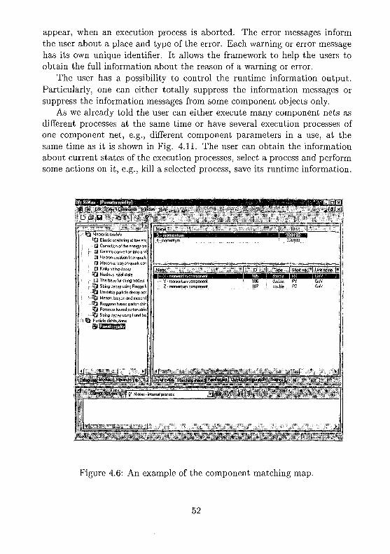
appear, when an execution process is aborted. The error messages informthe user about a place and type of the error. Each warning or error messagehas its own unique identifier. It allows the framework to help the users toobtain the full information about the reason of a warning or error.

The user has a possibility to control the runtime information output.Particularly, one can either totally suppress the information messages orsuppress the information messages from some component objects only.

As we already told the user can either execute many component nets asdifferent processes at the same time or have several execution processes ofone component net, e.g., different component parameters in a use, at thesame time as it is shown in Fig. 4.11. The user can obtain the informationabout current states of the execution processes, select a process and performsome actions on it, e.g., kill a selected process, save its runtime information.

3 Hadiomcrriodete

^ 3 Elastic scattering at low ant

Q Correction of the enetgy-mo

[3 Gamma convertion into a vi

C3 Hadton cteation Iiorn quark

13 Meson oi buyon quark con

E3 Kinky stihg decay

^ 3 Nucleus initial state

C3 The base (w siring models

^3 String decay using Reggefi

^ 3 Unstable particle decay act

1^3 Meson, baryon and meson-1

GCj Reggeon based parton sttr

• Q Pomwon based parton slrin

^3 Sliing decai' using Lund fra

| Paibcle distributions

4 momentum

Name

'•• Y-trcjmenturncomponerrt• Z - momentum component

106• 1D7

H

I'U

Iwarn

BBnaadoubt:double

ID I|i|ii|iilH

300103

I SMn.

naaaPYFZ

iMtrme 1

GeVGsV

Figure 4.6: An example of the component matching map.

52

4.5 Working on the data files

The system user can look through the data event configuration (see Fig. 4.12)and data (see Fig. 4.13) written in data files. The whole data events as wellas their separate channels can be selected through the data configurationview. We refer it as a structural data selection. After the selection onecan perform different operations on data, e.g., copy, cut, protect againstcomponent access, etc.

4.6 Working on the histograms and plots

One- and two-dimensional histograms with fixed partitions can be createdand visualized as well as two-dimensional plots (see Figs. 4.14 - 4.16). The

£<*

FS- l f i Hadronic models

^ Elastic scattering el low a r c

G) Correction of the energy-mo

C3 Gamma converlion into a vt

01 Hadron creation from quaik

[ 2 Meson ex batyon quark con

13 Kinky string decay

1^3 Nucleus initial stale

Q The base f a string models

i ? | String decay using Heggefi,

E& Unstable particle decay ace;

1^3 Meson, baryen and mesoni

^3 Reggeon based parfonsdvr

1 3 Pomeion based paitonstrh:

*?D String decay using Lund fta

3 % Paiticte disUibutions :

- ^ Pseudorapkity

1 PomeronPartonStringModel Input2 PomeionPartonSttingModeHnput

\SN2013011\ParticlB\MovingPoint201302ParticleVMoyingPoint_

4 PometonP«lpnS(ringModel Diltpit SSN2D13015\Pa(licle\MovingPoint

THB IShortna-

X - component of Lorentz m ..Y • corrponenl d Loietil; momentumZ - competent of Lotentz momentum

105 double PX106 double PY107 double P2

GeVGeVGeV

RMOJ

Figure 4.7: An example of the observed matching configuration.

53

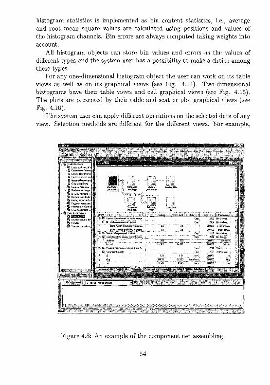
histogram statistics is implemented as bin content statistics, i.e., averageand root mean square values are calculated using positions and values ofthe histogram channels. Bin errors are always computed taking weights intoaccount.

All histogram objects can store bin values and errors as the values ofdifferent types and the system user has a possibility to make a choice amongthese types.

For any one-dimensional histogram object the user can work on its tableviews as well as on its graphical views (see Fig. 4.14). Two-dimensionalhistograms have their table views and cell graphical views (see Fig. 4.15).The plots are presented by their table and scatter plot graphical views (seeFig. 4.16).

The system user can apply different operations on the selected data of anyview. Selection methods are different for the different views. For example,

Figure 4.8: An example of the component net assembling.

54

the user may use a mouse to select the content of bins for a table view of ahistogram object and for the graphical views we offer a brush tool.

We would like to make a remark concerning histogramming facilities thatprovides by the NiMax system. Many of the facilities of the HBOOK package[2] (de-facto a histogramming standard for high energy community) as wellas a number of useful extensions are offered for the NiMax users, if they aredealing with the histogram pre-defined data events. It is important to un-derstand that the histogramming facilities are offered through the histogramviews. Thus, some of the HBOOK functionalities such as a histogram re-binning and histogram fitting are not discussed here. These facilities areconnected with new object creations that are a component privilege. Wehave to develop a special component or several components for this purpose.

£dj VV-vi Camai IP

D & a *> t> t

t j Elas'cscaile-rig^l'(3 Coiii*cicn ol the entQ Ganms convn icn n

Gi Me-on c* bJiyon QLUG Krb lir-pgd'c^

t f t Nuckii. r*ol-Ja!cQ r i vb i elwutrjm

t 3 PejgeDrbs-edpatc££3 Pumetuv ba-ed [wile

f}3 liftSEsrSiRl

Pa H-S/<S>

C^ôv^ MOQJK 1 Hic£f^*¥ f

5

]

1

i*

B

five

3 mowntun

^ -no-Krtun

- Ptnvi

- S Pi

- 61

\rptt fine* j H

3S

1

wiPiilcnStrir

[Pal. lei

—

" re*D i

Cm

t>Mcde! In?

Q Momjpoir.

- Xp

- fp

- Zp- Tp

- X- Y

- Z- E™

Mchmws

f

o «er,

0'ition

.o N f eTM102

OT10'

1 P

<; P

3 F

•I 'j 10 1

j 2013001

•013011

30

10

1C1

102

101

104

d Lee 1U5

ccrr*otvrt c/Lore "OS

c c n w n t rfl.cn" 07

103

H i

KTHfrP

jiier rP

orr*syp

T ^

Grsjp

Group;

Group

cyvj[«

d.ijr>

duubk

dooblfCttWe

txWlnprf SNÛlWil^Pa

..cos,,,*.

| SWiu.SH'J

PifcV-

•,

zI

^

FZ

E

ccrfQ |0p-

j Urflrww ! M J |E«i-nl

'^-ire l e 012

f^m. le 012

ten leOIJ

feirr. 1e012

reV 10C0

GA1 IOOII

C«V 10CO

GeV 1000

_ " -

i.l-0( v r ^cn l

Tvpo-oj

["1

[-1

8

S

8

e3

88

3

j

-1

J-1

1

Figure 4.9: An example of the net configuration tuning.

55

4.7 Obtaining a help

Help sub-system has been developed for the Windows platforms by applyingthe HTMLHelp Workshop [3]. Such sub-system is needed to help systemusers and potential model developers. The help sub-system from a hadronicmodel developer point of view can be considered as a platform to explainhow to develop model codes. There are two types of the help: the systemhelp, i.e., help information to assist in the system usage, and the componenthelp (see Fig. 4.17). The help topics related to the NiMax system describehow to handle components, how to process data, etc. The help topics relatedto a particular component include the information about the componentparameters, its input maps, its output events, etc (see Fig. 4.18).

The navigation through the help documentation and search of the neededinformation can be done using contents and keywords.

Hadronic models

££2 E aslic scatleiing at tow

0 Cuieciion cMhe energy

£3 Gemma conveMion into <

Ejj Hodion cicoticn horn qj

&3 Meson a b*yon quark <

O Kmty slrng deây

^3 Nucleus initial stale

• The base for siring mode

2013100?m 3200

4>> s will tun wilhin the -contextJM I

^ 3 Urstabls article d e w

^ j j Meson, bvyor, end mcsi

*?3 Reggson bassj patten:

*£ ] Pomeron based palon t

^ 3 Siring decay using Lurxi

© Palide distilbutions

EcmNurter

pI m p s - i n . i'- i

10 ZA3

\i-tnA 'i&TX (f MJt p

ID 2C133S!

Jtl

Figure 4.10: Reset of the net execution environment.

56

Hr fo r i c models

1 & Clastc scatlemg a( tow

E3 Collection of the aieigy

Qj Garnmaconvertionirtlo c

£3 H a i w c a t i o n from q<v

E3 Mescn oi baiy:n quark c

GJ Kinky diinQ decay

Q The base fo; st;ing mode

^ 3 Slrhg decay using Rcgc

- % Unstable paibcle d e c ^

1 3 Meson, baijcn and mesi

1 3 Reggem based paton

^ Pomeion based paitoos

^ Sbr^ dewji -jsing Luid

Paiticte dstjibu!! m

|)3 Pseudoiapidit>

Piqectla chatgePicjectle nimba of nuclsonTarget chaigeTarget nwnter ci nudeonEcmNumber cf cvenlsImpact parameter X yalu'1

Imoacf paranvlei Y value

j ; PiOTeiOTbasedpailoi s

Px = -0.000105172 Py = l.S428e-005 ?z =H-hadcon - 21936 Event:

t = -7.37945e-0Q5 Py = 0.000146305 ?z =H-hadcon = 21674 Euent: (

Pomcron based porton itring rrodd

Pomeron based Darton siring model:!

Porneran based pji lon s!ring model:2

Pometcn based parlon siring modd:C

"3

H-hadc< 213S3 Event:I

Figure 4.11: Several nets are executed as separate processes.

57

E * S » Commands Wrutas

ID TThortrm, 1 Ueinvue I3 Hadrwwc models

I?3 Elastic scattering at low

D) Correction of the energy-

d Sanima conveilion into <

E3 Madron crealien from qu

Q Meson OJ ba i jw quark c

• Qj KirJiy string decey

££) Nucleus initial state

Q The base for siring mod?

. I?3 Stiing decay ust.ng Reg;

^ ! Unstable particle decay

^2 Mesci. baryon and me$i

<& Reggeon based parton;

^2 Pomeron based parton s

^ String decay using Lund

% Pariide rtistribulions

PomeronPaitonStrmgModel InputPomeronPaftonStrmgModel Output

Moving point

2013001 Noimal SUM Event2015002 Noimal SUN Evert

30 . (Group] Paibcte10 : Group Movng..

• - Mass- Charge

i ^ Proiectile residual1 S Tatgct residual

Siring decayer input: vm Parton

- Encodrsgi Ar.!ipailon•: S Padon

;- S Moving point--X-posit ion

302 double M303 double Q

2013015 Group SIJ2013..2013016 Group SH2013...

GeV

20090001 • Normal: 20090011 • Group

30120D90012

20

intGroupGroupGroupdouble

SHN EventS(J2009..

Moving..

T-posB;onX • component of Loren.

Z - component of Loien.

104 • double T105 double PX

GeV

7|Da(a

ilR e a *

Figure 4.12: Data selection by means of the data configuration view.

58

I D Tjj Hadronk: models 1

^ | Elastic scatler'ng at low i

13 Correction of the energy-

E2 Gamma conveition inio. j

E3 Hadron crealjon from qu i

[3 Meson oi baiyon quark c!

Q Kink>i string decay :

^ Nucleus rvtial slate

Q| The base foi stirig rnodt

^3 Strifig decay using Regj;

• ^ Unstable pailide decay

• ^ 3 Meson, basyon end roes':

- ^ | Reggeon based parton; ''•

•f| Pomefon based patons^

^ 3 Siring decay using Lund:

Paiticle dslritwtions !

^ Pscudofapidilv

1 i PornejonPa-lof^tringModd OUpul2 o PomefonParionStringModel Oufput

PomeronParlonStrmoModd OutputPofne/onPartonStnngModel Output

PomeronPaitonStringModel Output

Hstm...* P*ticle[ 21594]- ' Pfojeclte residua!

5 ParticfelG)

* [0!4 [ 1 ]

X-positionY-positianZ-positionT^wsitionX • component ol Lotentz momentumY - component ol Loienlz momentun2 • component ol LaenU momentumEnwgy

2013002 ; Normal2013002 i Normal

2013002 : Normal2013002 Normal

1215341

[61

785335•2087310.783862

0-0,1451380.0498142

539815399816

farmtornfern*(MiriGeVGeVGrVGeV

Figure 4.13: An example of the selected data.

59

D£te_£d» Sew EsmMnds ifmiow Help

' — - — - •"=• - .si

' Q Elastic scatteiing at 1(

'• '•••••• Q Correction of the ene

i (3 Gamma convertion in

; 13 Hacfcoti creation from; : •••• C3 Meson OE baryon qua

E3 Kiriky siring decay

: ; • !?3 Nucleus initial stale: CO The base (or string m

* O Stiing decoy using R>1 E - t?3 Unstable particle dec

^ 3 Meson, baryon and n

^ Reggecn based p#ic

;- l?2 Pomeion based part: ;

^3 Siring decay using Li :

K ^ Partble distributions: - ^ 1 Pseudorapidty

Caleoorv iModulel Htaarehi'l

N bn | Corter* 1 ••

22 33823 47424 55425 703

28 35323 103530 : 1183 :•.

32 1627 • ;33 1900 ;•

35 299437 358233 408839 : 4889

4

10 61451 : 6892

i2 7543 "3 78144 7660•5 7288 :.6 7088.7 653518 5885 r j

eooo

7000

6000

5000

-WOO

3000

1000

- • • • -

r\ nJ V I T . . . .i r I

. .: : I " L" " I ' • L ' ': : J 1 . J 1

J V 1

: • ! • • • [ •

. J 1 .....I • 1

J l\ I

r 1 '. f 1

/ • . . \ . . .

: t ^ ^

Pane |

- 1 Cutsnt process. | ; Pseudoiapidily

::

d

li

Figure 4.14: An example of the one-dimensional histogram views.

60

j Hadortc models^ 3 Elastic scattering at low13 Cwterfion of the eneigy-mo

. Q Gamma convertion inlo a vt• -- [3 Hadtoo weationfrom quark

• Q Meson M bayon quaik con= - E3 Kinky stiing decay\-^l Nucleus initial state

• Q The base lot stiing modelsr -^ j l Stiing decay using Regge d• J& Unstable paiiide decay tec

%3 Meson, faaiyon and meson-1i - - ^ Reggeon based parton strr• ^ Pometon based paiton sltin

^3 Stt'rxjdecayusingLundfraPaibde dtstiibutions^ PseudotapitBy

J ±t

"Hi

lilili

| ; Nucleus r U s

- I -ti

Figure 4.15: An example of the two-dimensional histogram view.

61

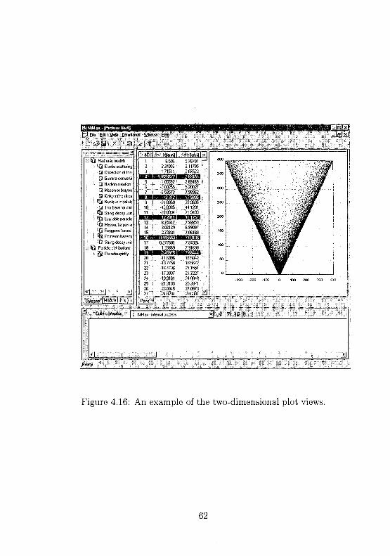
-l%& Hadronic models

!?3i Elastic scatlano

| • Q Coiieclion of the ,

i Q Gamma conveilit

. ;- Q Hacion a c t i o n

i •• E3 Meson of batyon

; E3 Kinky stiing dew

! ^ 3 Nucleus initial sic:

i • Q The base for siir

• ££a Sling decay usar

;• t?2 Unstable particle

•••'O Meson,baiyona; : l?2 Reggeon based

! ^ Pometon based f

: tfjl Sting decay usir

3 © Particle distributions

Xlfami I Vffwi1 6538 5 767912 224002 2117953 171511 207523

9 -31.8053 32959510 43.0365 4< 129111 " -708934 719493

Figure 4.16: An example of the two-dimensional plot views.

62

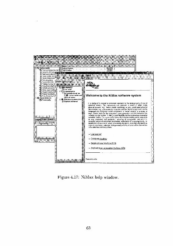
Q H*Jo«i aeabcn Iran• Metco a twiycn quaQ K>*v stnig decoy

% Hucleuc nbd stateQ T he bas«l« siring ir>,

fBl Sbing decî using Ht!

ft Umt(te parScte decift Meiai.b«ycnarjdnft ReflgaoobwedwilC!ft PcmaonbaiodpMoft String decay iciig U;

& Patide dmbuticm

Otttrtprocait j ; t

]j Ccmponert 9al«y

• ^ Hadtork modeh vij|] List ol tnadi«i

Welcome to the NiMax software system

H is designed lo support a componem approach la iho development and use ofnumerical models. The components can repiesenl a mode! of either singlephysical process, e.g., hadion elastic scattering, ot very complicated physicalphenomenon, e.g., uHra-ielatrvislic heavy-ion collision. Model components can becomposed into composite model components cr mcde! projects in a variety ofways. Several loots foi the component codes generation and their extension areincluded into the system. It offers a great flexibility for the construction of powerfulnumerical models. The system offers many GUI services making user's session lobe very convenient and productive: launching of components and projectscontrolled edition of component parameters, substitution of sub-components, re-organiialion of component output, assembling of projects, execution of projects asseparate processes, selection, histogramming and visualization of the data writtenin the data files and many others.

. User manual

. Component Gallery

. Graphical user interface (GUI)

• Application programming interface (API)

Figure 4.17: NiMax help window.

63

Elastic scattering at low andhigh energies

This model component can be applied to simulatemeson-nucleon and baryon-nucleon elastic scatteringsat low and high energies.

Home page | Module list t Application domain tree 1

'••±1

Figure 4.18: An example of the component description.

64

Bibliography


[2] HBOOK Statistical Analysis and Histograming Reference Manual,CERN Program Library Long Writeups Y250, CERN Geneva, Switzer-land, 1998.

[3] Kruglinski D. J., Shepherd G., Wingo S. - Programming MicrosoftVisual C++, Fifth Edition, Microsoft Press, 1998.

65

Chapter 5

Summary andacknowledgments

5.1 Summary

We have described a new approach to the development and use of numer-ical phenomenological models in high-energy physics. It is the componentapproach, when a complex numerical model is composed from simpler modelcomponents that are included into application modules.

We have formalized a standard component or a component model by theseparation of a component interface part and component algorithm part. Anycomponent is thought as a set of standard interfaces between its numericalalgorithm and the outside world.

We have described a unit of configured data: the data event. A compo-nent may produce data events, write them in a data file for further analysisand visualization, read data events from a data file and receive data eventsfrom other components.

Within the approach we offer a possibility to compose several componentsinto a composite component or component net as well as different tools todevelop a new specific components. It provides a great flexibility for theconstruction of powerful and realistic numerical models.

Each particular component can be tuned and different implementationsof the component algorithm can be interchanged at runtime enabling a modeluser to obtain needed model properties without redesigning of a model andwriting the model code.

To support this approach we have developed the NiMax software system.The NiMax system is an object-oriented software written in C++. It isoriginal and unique system. Its central part is a framework that controls

66

all the system's internal processes and provides an interaction between thegraphical.user interface (GUI) and rest of parts.

The framework offers many GUI services to have a convenient and pro-ductive user session. For example, the user is able to launch required com-ponents and component nets. He or she is able to perform a controllededition of component and sub-component parameters, substitution of sub-components within a composite component, re-organization of component,and sub-component outputs. The user can assemble and edit different com-ponent nets and execute them as separate processes. The user is able toperform structural, analytical and graphical selections of the produced datathat have been written in the data files. He or she can build and visualizehistograms and plots.

The NiMax system offers many tools to. make a productive work of thecomponent developers. It includes different wizards of the component codesand component documentation. It includes libraries of the application datatypes and data transfer classes. These tools and libraries facilitate the de-velopment of interface and algorithm parts of the components. Workingon them we assume that the model component developers should work oncomponent numerical algorithms and each component numerical algorithmcan be developed independently from other component numerical algorithms.Component functionalities are extensible by the inheritance mechanism andcomponent codes are re-usable by the component aggregation.

Several concepts of our system have no analogies among the existingsoftware systems. One of them is the component aggregation mechanism.It allows C++ developer to write a large size component code by re-usingof ready components without coding limitations. For the outside world anaggregating component looks like a single component. However, its user hasthe access to any sub-component and is able to modify the algorithm of thecomposite component by a sub-component substitution. Another one is thematching of data event configuration. It allows us to organize a collaborationof independent components by transferring of complicated data structuresbetween these components. The component developer is not required to learnor use the system or component classes with the aim to support componentcollaboration. The matching of a data event configuration offers a possibilityof a structural selection of the data that is written in the data file.

An additional idea of pre-defined data events and pre-defined data chan-nels facilitates data visualization and data analysis and opens a possibilityfor an independent extension of the existing user interface and for the devel-opment of special (for different application domains) user interfaces.

The format of the developed data file allows storage of a large bulk ofthe differently structured data and fast navigation through these data. The

67

data file, data file views and data file control and navigation methods may bethought as an independent data file system for the processing of large datevolumes and having its own applications.

The html based help sub-system is a part of the NiMax system. Helptopics include descriptions that related to our system and implemented com-ponents. The navigation through the help documentation can be done usingcontents or by keywords. The help sub-system can be use for an informationexchange in a separate from the NiMax system.

We have applied the NiMax system for a particular class of the numericalmodels: the Monte Carlo event generators for high-energy physics. With helpof the NiMax system we have developed hadronic modules. They includemany MC model components that allow their user to perform a simulationof the particle and nuclear interactions at wide high-energy range and for alarge set of projectiles and targets.

The NiMax system can be used in different application domains. First ofall, it is suitable for the applications based on a use of complicated numericalmodels that generate data. We have started the development of applicationmodules to perform computer simulations of the radiation transport in dif-ferent media. Besides of the numerical simulations it can be applied for thestructural (based on the data event configurations), analytical (based on theuse of numerical models) and graphical (based on the data visualizations)analysis of the data obtained from different sources.

5.2 AcknowledgmentsWe are thankful for our colleagues from the Laboratory of High Energiesof the Joint Institute for Nuclear Research, Dubna for collaborations. Wewould like to thank our colleagues from the Physics Department of JyvaskylaUniverstity, Finland for their interest in the NiMax system and numerousdiscussions about the system features.

Chapter 6

Hadronic modules

6.1 Particle structure components

6.1.1 Particle propertiesParticle properties have been tabulated. These tables keep the properties oflight quarks and antiquarks (u,d and s) as well as the properties of diquarksand antidiquarks that are consisting of light quarks and antiquarks. Wehave tabulated the properties of a gluon, photon and leptons (e*, JJ^ andve,n)- We have also tabulated the properties of Jp = \+, | + baryons andbaryon resonances as well as JPC mesons states: (0"+),i.e., TT,K,T] and 77'and (1 ),i-e-, P,K*,UJ and <j>. J, P and C denote a spin, parity and chargeconjugation, respectively. The full baryon-antibaryon symmetry is assumed.

In the case of a resonance production the resonance mass m is determinedaccording to the Breit-Wigner distribution:

The particle properties, pole masses m# and total decay widths T(mR) aretaken from the Review of Particle Properties [1], [2], [3], [4].

6.1.2 Baryon and meson splittingTo perform the simulation of a string excitation we need to split baryon (an-tibaryon) and choose valence quark (antiquark) and diquark (antidiquark).In the case of a meson we split it into valence quark and antiquark (for neutralmixed mesons this splitting is performed according to the quark mixing prob-abilities). We determine the probabilities of the baryon (antibaryon) state(quark (antiquark) and diquark (antidiquark) with given spin and isospin)

69

Baryon typePn

E°£~

T:0

A°A++A+A0

A"E*+£*°£*-H*°7 7 * —

n-

l/3ud\\S -

1/Zudoos H

Quark contentl/3uund + l/6udnu + l/2udoou\/£>udnd + l/2udood + l/3ddnu

- 1/I2usnd + l/4usood + 1/I2dsnu + l/4ds00ul/3ddus + l/6dsnd + l/2ds00dl/6dsns + l/2ds00s + l/3ssndl/6usns + 1/2USOQS + l/3ssnu

- l/4usnd + l/12us00d + l/4dsnu + 1/I2dsoouUUuU

l/3uuud + 2/3udnu2/3udnd+l/3dduu

dd\\d\/3uuns + 2/3usnu

l/3udns + l/3usud + l/3dsnu\/3dd\\s + 2/3dsi\d

2/3ds\\s + l/3ssndSSnS

Table 6.1: Baryon quark contents,states.

Diquark indices indicate spin-isospin

from 5(7(6) symmetric baryon wave functions. These probabilities are givenbelow in the Table 6.1.

We can also use these probabilities to sample baryon or baryon resonancein the course of a string fragmentation, assuming that a valence diquark(antidiquark) keeps its spin and isospin values during the reaction.

6.1.3 Gamma conversion

To calculate high-energy interaction of the real or virtual photon with anucleon or a nucleus, we convert it into a vector meson or meson type system[5].

We consider the following kinematics variables for 7-nucleon scattering:the Bjorken's x variable is defined as x = Q2/2mu with Q2, v and m arephoton virtuality, photon energy and nucleon mass, respectively. The totalenergy squared of the 7-nucleon system is given by s — Q2(l — x)/x + TO2.We restrict our consideration to the range of small s-values and Q2 is muchless than s.

70

The Generalized Vector Dominance Model (GVDM) [6] assumes that avirtual photon fluctuates into intermediate qq-state V of mass M that maysubsequently interact with a nucleon N. Thus, the total photon-nucleoncross section can be expressed by the relation [5]:

2 dM2D(M2) J Q ) ( j(6.2)

where the integration over M2 is performed between M2 = 4m2. and M2 = s.Here aem = e2/4n = 1/137 and ^-system mass squared distribution is given

and

R ( M }

where e is the squared charge of a quark with the flavor / . e is the ratiobetween the fluxes of longitudinally and transversally polarized photons.

The Monte Carlo procedure of a gamma conversion can be outlined asfollows:

• At given s and virtuality Q2 sample the mass M2 for a hadron qqfluctuation according to the Eq. (6.3);

• Sample its flavor according to the statistical weights: wufl = 1/2, wd^ =1/4 and wsS = 1/4 that are derived from the Eq. (6.4).

71

Bibliography

[1] Particle-Data-Group, Phys. Rev. D45 1342 (1992).


[3] Particle-Data-Group 98, Eur. Phys. J. C3 1 (1998).

[4] Particle-Data-Group 2000, Eur. Phys. J. C15 1 (2000).

[5] Piller G., Ratzka W., Weise W., Z. Phys. A352 427 (1995).

[6] Bauer T. H., Spital R. D., Yennie D. R., Rev. Mod. Phys. 50 261(1978).

72

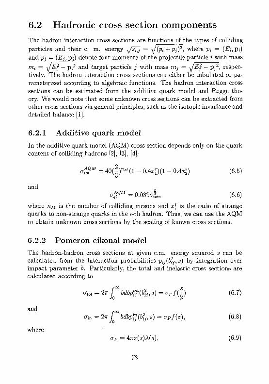
6.2 Hadronic cross section components

The hadron interaction cross sections are functions of the types of collidingparticles and their c. m. energy ^fsTj = J{Pi+Pj)2, where pi = (Ei, Pi)and pj — (Ej, pj) denote four momenta of the projectile particle i with massrrii — JEf - p;2 and target particle j with mass rrij — JEj — Pj2, respec-tively. The hadron interaction cross sections can either be tabulated or pa-rameterized according to algebraic functions. The hadron interaction crosssections can be estimated from the additive quark model and Regge the-ory. We would note that some unknown cross sections can be extracted fromother cross sections via general principles, such as the isotopic invariance anddetailed balance [1].

6.2.1 Additive quark model

In the additive quark model (AQM) cross section depends only on the quarkcontent of colliding hadrons [2], [3], [4]:

4SM = 40( | ) n " (1 - 0.4a;J) (1 - 0.4*5) (6-5)

and 2

afM = 0.039^, (6.6)

where nM is the number of colliding mesons and xf is the ratio of strangequarks to non-strange quarks in the i-th hadron. Thus, we can use the AQMto obtain unknown cross sections by the scaling of known cross sections.

6.2.2 Pomeron eikonal model

The hadron-hadron cross sections at given cm. energy squared s can becalculated from the interaction probabilities Pij{bfj,s) by integration overimpact parameter b. Particularly, the total and inelastic cross sections arecalculated according to

roo 7

atot = 2K bdbpf{bl,s) = oPjQ (6.7)

^ %l , (6.8)

wheres)A(s), (6.9)

73

and

In the Regge-Gribov approach [5], [6] the probability for an inelastic col-lision of hadrons i and j as a function of the squared impact parameterdifference b2j = (fej — bj)2 and s is given by

oo

Pij(k - bjt s) = c-l[l - exp {-2u(bl,s)}] = J2Pi?& ~ bj, s), (6.11)n=l

where

p&>& - lh s) = c-1 exp {-2u(bl, s)}[^fK (6.12)

is the probability to find n cut Pomerons or the probability for 2n stringsproduced in the inelastic hadron-hadron collision, if we assume that each cutPomeron can be substituted by two strings. These probabilities are definedin terms of the amplitude (eikonal) of hadron-hadron elastic scattering withPomeron exchange:

«(6?-,s) = ^ e x p [ - ^ / 4 A ( S ) ] . (6.13)

The quantities z(s) and A(s) are expressed through the parameters of Pomerontrajectory aP = 0.25 GeV~2 and ap(0) = 1.0808, and the parameters ofPomeron-hadron vertex F?P and jp:

z(s) - ^ ( ^ o ) 0 " ™ - 1 (6-14)

X(s) =RP + a'Pln{s/s0), (6.15)

respectively, where SQ is the dimensional parameter.In the equations (6.11,6.12) the so-called shower enhancement coefficient

c was introduced to determine the contribution of diffractive dissociation [6].Thus, the probability for diffractive dissociation in hadron collision can becomputed as

p%{bi - bj, s) = — [$*& - bjt s) - pijfa - bj, s)}, (6.16)c

wherepf{bi - bj, s) = (2/c)[l - exp{-«(6*., s)}]. (6.17)

74

The Pomeron vertex parameters are found from a global fit of the total,elastic, differential elastic and diffractive cross sections of the hadron-nucleoninteraction at different energies.

For the nucleon-nucleon, pion-nucleon and kaon-nucleon collisions we haveobtained the next values of the Pomeron vertex parameters and shower en-hancement coefficients: R%N = 3.56 GeV~2, 7 £ = 3.96 GeV~2, s$ = 3.0GeV2, sg = 1.4; Rf = 2.36 GeV~2, i"P = 2.17 GeV~2, s% = 1.5 GeV2,cn = 1.6; R2

PK = 1.96 GeV-2, 7 £ = 1.92 GeV-2, sf = 2.3 GeV2, cw = 1.8.

These values can be used to describe properly the total, elastic and diffractivecross sections.

6.2.3 Single diffraction cross sectionThe proton-proton single diffraction cross section was parameterized in paper[7]

oSD{s) = (0.68 ± 0.05) (l + — ) In (0.6 + 0.1s), (6.18)s

where s is the total cm. energy squared.

6.2.4 Baryon annihilation cross sectionTo calculate the baryon-antibaryon annihilation cross sections we follow theapproach [4]. In this approach the same initial energy dependence is usedfor all baryon-antibaryon cross sections. The different baryon quark contentsare taken into account by scaling factor obtained from the AQM [2], [3]:

AQM

(6-19)NN

where the antiproton-proton annihilation cross section <7?™n is parametrised[8] by

and the antiproton-neutron cross annihilation cross section is treated identi-cally. The parameter values are CTO = 120 mb, so = 4m^, A = 50 MeV andB = 0.6.

75

Bibliography


[2] Levin E. M., Frankfurt L. L., Pisma ZhETP 3 105 (1965).

[3] Lipkin H. J., Sheck F., Phys. Rev. Lett. 16 71 (1966).

[4] Bass S. A. et al, Prog. Part. Nucl. Phys. V. 41 225 (1998).

[5] Abramovskii V. A., Gribov V. N., Kancheli 0 . V., Sov. J. Nucl. Phys.18 (1974) 308.

[6] Baker M. and Ter-Martirosyan K. A., Phys. Rep. 28C (1976) 1..

[7] Goulianos K., Phys. Rep. 101 169 (1983).

[8] Koch P., Dover C. B., Phys. Rev. C40 145 (1989).

76

6.3 Particle decay components

6.3.1 Particle decay simulation

Particle decay channels are sampled using the partial decay widths T(m),which depend on the masses m of particles. All particles are considered asnon-polarized particles. If a resonance is among of the outgoing particles,its mass is determined according to the Breit-Wigner mass distribution. Allpole masses and partial decay widths are taken from the Review of ParticleProperties [1]. If an exit channel contains two, three or four particles, thenthe respective TV-body phase-space is taken into account during the samplingof particle momenta.

The Kopylov's algorithm [2] is used to sample product particle 4-momenta.We would stress that the Kopylov's algorithm gives a possibility to take intoaccount resonance decay matrix elements.

6.3.2 N-body decay algorithm

We can write the n particles state probability as

- Pn)\M\\ (6.21)t = l

where Pn = (P n , En) is the decaying particle 4-momentum and M(p\,p2, •••,pn)is the reaction amplitude, which depends on the 4-momenta pi of products.

We know the sum of produced particle masses

Mn = E m i (6.22)i=l

and cm. system kinetic energy

Tn = Mn- txn, (6.23)

where Mn = \JE%, — P% is the invariant mass of the system.Performing integration of the probability expressed by the (6.21), one

can obtain different particle distributions. The integration over all set ofvariables S can shortly be written as follows

W= f §(S)dS, (6.24)JD

where $(S) can be considered as the weight of n-particles production event.

77

The Kopylov's algorithm is based on the choice of a set of variables S\:Tk, rjk and (frk instead of particle 4-momenta to perform the integration ofdW. The integration range Dx over these new variables is simple. Angularvariables are inside 1 > % > — 1 and 2-K<f>k > 0, where k = n, n — 1,..., 2, andkinetic energies of the systems with some numbers of particles are orderedaccording to Tn > Tn_i > ... > T2 > 7\ - 0. Further substitution of thevariables Tk, r]k and <pk by the set variables S2: £k, Ik and (5k that are limitedbetween 0 and 1, creates an unit hypercube from the integration range D2:

(6.25)2 2

Two sets of variables Si and S2 are related to each other:

rjk = 2f3k — 1, k — n,..., 2 (6.26)

The event weight $(Si) [2] is

{^{n — i)) k=2 \/lk - ifc_!

where F(:r) is the gamma function and pk is the 4-momentum of k-th particlein the rest frame, 0k, where Tk = 0.

As one can see from the Eq. (6.25) the variables £/;, 7^ and /?£ canbe considered as random numbers distributed between 0 and 1. Thus, togenerate particle momenta we can apply the next recursive procedure [2].

1. Sample ^ _ i according to the distribution

where functions F(£k) have maxima Fmax — F((3k — 5)/(3fc — 4)), andcompute Tk-\ = Tk£k-i- If & = 2, then Tk-\ should be set to 0 inaccordance with the definition of the rest frame Ok-i-

The functions F{x) are sharp functions at large values of k. At thelarge k we can use another method of the sampling with a tabulation[2]. In this case for uniformly distributed between 0 and 1 randomnumbers at-i we have to solve the equation

C f c-i(^-i) = a*_i, (6.29)

78

whereJt-5

f U WA (: 2 . /T _ £.(6.30)

and find the value of £*_i. Ck(^k) are tabulated smooth functions. Alinear interpolation can be applied to find the function values at theintermediate points.

2. Compute the total energy

Qk = {Ml + m2k- Ml_x)l1Mk (6.31)

and absolute value of 3-momentum

p* = VÎ - ml (6.32)

for fc-th particle in the rest frame, 0k, where

ptk—i = /ifc — vn,k (6.33)

andMk-i = /;*_! - TA_X. (6.34)

3. Sample the direction of ft-th momentum p^, i.e., sample the azimuthaland polar angles according to <pk = 2ix"fk and cos 9k = 2/3^ — 1, re-spectively. The 7^ and /3k are uniformly distributed between 0 and 1random numbers.

4. Calculate the A;-th particle energy

uik = fca,——k- (6.35)

and its 3-momentum

in the observer frame.

5. Calculate the total energy Ek_\ and 3-momentum Pfc_i of the systemwith k — 1 particles:

Ek—\ = Ek — uik, (6.37)

Fk-x = Pfc - p*. (6.38)

79

If k = 2, then we can check that mx = ^jE2 - P\, where pi = P i and

As result of the outlined recursive procedure we know the momenta of allproducts and can calculate the event weight (6.27).

Finally, if <3?(Si) < ^max, where £ is a uniformly distributed between 0and 1 random number and §max is a maximal value from the <&{Si) set ofvalues, we will accept the event.

We should note that in the non-relativistic case and for |M|2 = 1 the laststep, i.e., the test $(5i) < £,<fcmaX) is not needed [2].

We also should note that the outlined procedure can be used to calculatethe relativistic phase space volume W, i.e., to perform an integration overthe event weight (6.24) at \M\2 = 1. To perform this integration we need tofind an average value of the event weights for N events, where N —> oo. Thismethod to perform the integration is also efficient at \M\2 /= 1, if \M\2 hasno pole behavior. Thus, the Kopylov's algorithm can be used to calculatedecay widths and different particle distributions.

It also allows us to simulate the nuclear fragment production as result ofthe decay of excited nuclei.

80

Bibliography


[2] Kopylov G. I, The basics of resonance kinematics, Nauka, Moscow,1970.

81

6.4 String decay components

A colored string is stretched between flying away partons having color charges:a quark and antiquark or quark and diquark or diquark and antidiquarkor antiquark and antidiquark. From knowledge of the parton longitudinalP3i — Pzi and transversal pu — pxi, p2i — Pyi momenta as well as their ener-gies pOi = Ei, where i — 1, 2, we can calculate the string (string with partonends) mass squared:

M2S = p"pM =pl-p\-pl-pl (6.39)

where p^ — p^\ + p^ is the string four momentum and \x = 0,1,2,3.The string decay model components can be used to simulate decays of

the longitudinal q — q, qq — qq, q — qq and q — qq strings or kinky q — g — q,qq — g — qq, q — g — qq and q — g — qq strings.

It is convenient to perform a simulation of the string decay in the stringrest frame, with string end partons are moving along z-axis. Finally, after thestring decay we have to perform a backward Lorentz boost with the velocity—fin of hadron 4-momenta and their 4-coordinates and a backward rotationof hadron 3-momenta and 3-coordinates with the matrix R^1 (see below).

6.4.1 Cluster decay simulation

The procedure to model a cluster (small mass string) decay is suggested inthe papers [1], [2]. It is assumed that each cluster with mass Mc decaysisotropically in its rest frame into a hadron pair with masses M\ and M2 andspins J\ and J2 by pulling a quark-antiquark or diquark-antidiquark pairwith the quark (diquark) mass rnq. For a hadron, which is containing u, dand s quarks, the Jp = 0", I* meson and Jp — I"1", | baryon states areallowed. A decay channel is selected according to the probability:

Pdecay = Pflavor{Mc, mq)Pspin{Ju J2)Pps{Mc, MUM2), (6.40)

where the flavor factor is

n (M m ) _ j , ^ |

spin factor isPsPin{Ju Js) = (2Ji + 1)(2J2 + 1) (6.42)

and phase space factor is

+ M* + M* - 2(M*M? + MIMl + M\M\Ml)(6.43)

82

6.4.2 Longitudinal string decay

The decay of a string follows an iterative scheme:

string => hadron + new string, (6.44)

i. e., the string decay into a new string and hadron is modeled by meansof the vacuum quark-antiquark (or diquark-antidiquark) pair creation. Thevalues of strangeness suppression and diquark suppression factors are

u:d: s : qq = 1 : 1 : 0.35 : 0.1. (6.45)

Optionally, a possibility of a diquark breaking during the string fragmen-tation can be considered.

A hadron is formed randomly on one of the end-point of the string. Aquark content of the hadrons determines its species and charges. In thechosen fragmentation scheme we can produce not only the ground states ofbaryons and mesons, but also their lower excited states. If for baryons, thequark content does not determine whether the state belongs to the lowestoctet or to the lowest decuplet, then the octet or decuplet is chosen withthe probability that defined by spin and isospin of the diquark (antidiquark).In the case of mesons the multiplet must be also determined before a typeof hadron can be assigned. The probability to choose a certain multipietdepends on the spin of the multiplet. In the case of resonances their massesm are determined according to the Breit-Wigner distributions, where allpole masses and total decay widths are taken from the Review of ParticleProperties [3].

Zero transverse momentum of the created quark-antiquark (or diquark-antidiquark) pair is obtained by summing of equal and opposite directedtransverse momenta of the quark and antiquark. A transverse momentum ofthe quark is randomly sampled according to the probability (6.85) with theparameter a = 0.55 GeV""2. The produced hadron transverse momentum p t

is a sum of the transverse momenta of its constituents.The fragmentation function fh(z,pt) represents a probability distribution

for hadrons with the transverse momenta pt to carry a light cone momentumfraction z = z± = (Eh ± ph

z)/(E(> ± p«), where Eh and Eq are the hadron

and fragmented quark energies, respectively. pz and pqz are the hadron and

fragmented quark longitudinal momenta, respectively. The values of z arelimited between zîn and zâx. zînmax are determined by the hadron massrrih, constituent transverse masses and available string mass. One of the mostcommonly used fragmentation function is taken from the LUND model [4]:

] . (6.46)

83

One can use this fragmentation function for the decay of an excited string.One can also use fragmentation functions are derived in [5]:

f'^Pt) = [1 + <*£(< Vt >)](! - * ) ° J « * » . (6.47)

An advantage of these functions as compared to the LUND fragmentationfunction is that they have a correct three-reggeon behavior at z —> 1 [5].

To calculate produced hadron formation times and longitudinal coordi-nates we consider (1 + l)-string with the mass Ms and string tension K thatdecays into hadrons in its rest frame. The i-th produced hadron has theenergy Ei and its longitudinal momentum pzi, respectively. By introducingthe light cone variables pf = Ei± Piz and numerating string breaking pointsconsecutively from the right to the left we obtain p j = Ms, p? = K^zf-i ~'zt)and pj = KX~ .

We can identify a hadron formation point coordinate and time as the pointin space-time, where quark lines of a quark-antiquark pair that is formingthe hadron meet for the first time (the so-called "yo-yo" formation point [4]):

U = ^- [Ms - 2 £ pzj + Ei- Pzi] (6.48)

and coordinate

Zi = ~[Ms - 2 ]T Ej + pzl - Ei]. (6.49)2K 3 = 1

6.4.3 Kinky string decay simulation

For the kinky string decay simulation we have assumed a two steps process[6]:

1. Split the gluon g —¥ qiq~i and create two longitudinal strings;

2. Decay of the longitudunal strings qq~i —> h and qq\ —> h into hadronsh.

The production of q-^qi is considered similarly (the same sampling of quarkflavors and the same prdistribution for the quarks) as the production of qq-pairs during a longitudinal string decay. The g —> q\q~\ splitting function

fl{z) = z2 + (1 - z)\ (6.50)

where z = Eq

+Pl, have been derived by Altarelli and Parisi [7].

84

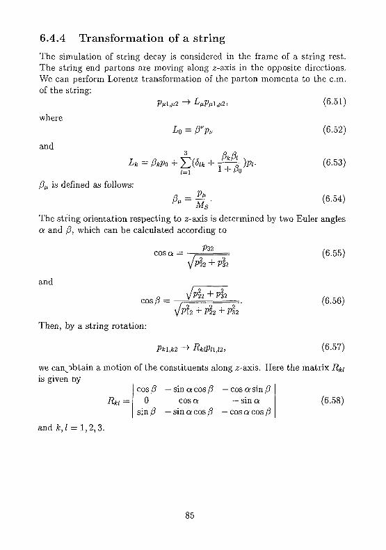
6.4.4 Transformation of a stringThe simulation of string decay is considered in the frame of a string rest.The string end partons are moving along 2-axis in the opposite directions,We can perform Lorentz transformation of the parton momenta to the cm.of the string:

P/j.l,fi2 ~^ •^/^P/il,/i2) (6.51)

where

and

Lo =

1=1, * I1 + P

is defined as follows:

Ms

(6.52)

(6.53)

(6.54)

The string orientation respecting to z-axis is determined by two Euler anglesa and 0, which can be calculated according to

cos a =P32 (6.55)

and

cos/? =\JPl2+P22+P32

(6.56)

Then, by a string rotation:

Pki,k2 -> RkiPn,i2, (6-57)

we canôbtain a motion of the constituents along z-axis. Here the matrix .is given by

cos 0 — sin a cos 0 — cos a sin 0

and k,l = 1,2,3.

0 cos a — sin asin 0 — sin a cos 0 — cos a cos 0

(6.58)

85

Bibliography

[1] Gottschalk T. D., Nucl. Phys. B214 201 (1983); B227 413 (1983).

[2] Weber В. R., Nucl. Phys. B238 492 (1984).


[4] Andersson В., Gustafson G., Ingelman G., Sjöstrand T., Phys. Rep.97 31 (1983).

[5] Kaidalov A. В., Sov. J. Nucl. Phys. 45 1452 (1987).

[6] Ali A, Pietarinen E., Kramer G., Willrodt J, Phys. Lett. B93 155(1980).

[7] Altarelli G. and Parisi G., Nucl. Phys. B126 298 (1977).

86

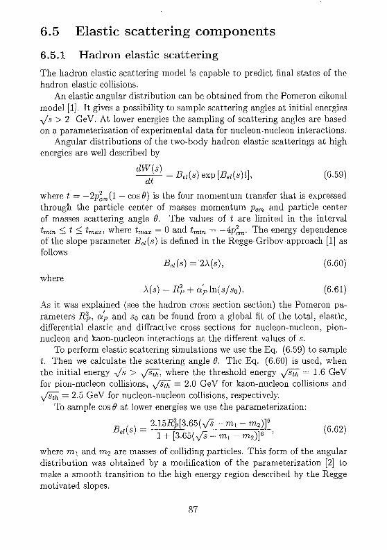
6.5 Elastic scattering components

6.5.1 Hadron elastic scattering

The hadron elastic scattering model is capable to predict final states of thehadron elastic collisions.

An elastic angular distribution can be obtained from the Pomeron eikonalmodel [1]. It gives a possibility to sample scattering angles at initial energiesy/s > 2 GeV. At lower energies the sampling of scattering angles are basedon a parameterization of experimental data for nucleon-nucleon interactions.

Angular distributions of the two-body hadron elastic scatterings at highenergies are well described by

^f = Bel(s)exp[Bel(s)tl (6.59)

where t — —2p2cm{l — cos#) is the four momentum transfer that is expressed

through the particle center of masses momentum pcm and particle centerof masses scattering angle 9. The values of t are limited in the intervaltrain < t < tmax, where tmax - 0 and tmin = -4p^m. The energy dependenceof the slope parameter Bei(s) is defined in the Regge-Gribov approach [1] asfollows

Bel(s) = 2A(s), (6.60)

whereX(s) = R2

P + dp ln(s/s0). (6.61)

As it was explained (see the hadron cross section section) the Pomeron pa-rameters Rp, aP and so can be found from a global fit of the total, elastic,differential elastic and diffractive cross sections for nucleon-nucleon, pion-nucleon and kaon-nucleon interactions at the different values of s.

To perform elastic scattering simulations we use the Eq. (6.59) to samplet. Then we calculate the scattering angle 8. The Eq. (6.60) is used, whenthe initial energy y/s > y/sth, where the threshold energy yfsth = 1.6 GeVfor pion-nucleon collisions, y/sth — 2.0 GeV for kaon-nucleon collisions and

= 2.5 GeV for nucleon-nucleon collisions, respectively.To sample cos 6 at lower energies we use the parameterization:

2.15i%[3.65(y/i - m i - m2)]6

B ( s ) =

where m,\ and m^ are masses of colliding particles. This form of the angulardistribution was obtained by a modification of the parameterization [2] tomake a smooth transition to the high energy region described by the Reggemotivated slopes.

87

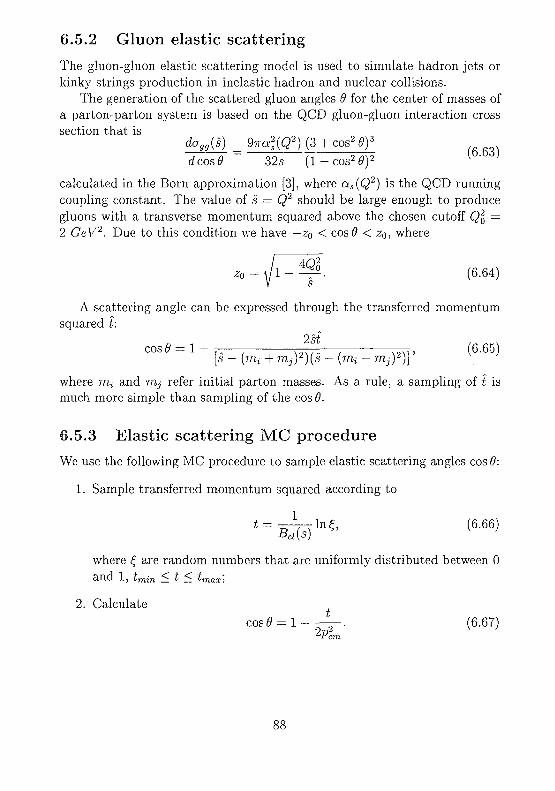
6.5.2 Gluon elastic scatteringThe gluon-gluon elastic scattering model is used to simulate hadron jets orkinky strings production in inelastic hadron and nuclear collisions.

The generation of the scattered gluon angles 6 for the center of masses ofa parton-parton system is based on the QCD gluon-gluon interaction crosssection that is

dogg(§) toctm (3 + cos2 9)3

dcos9 32s ( 1 - cos2 Of { 'calculated in the Born approximation [3], where as{Q2) is the QCD runningcoupling constant. The value of s — Q2 should be large enough to producegluons with a transverse momentum squared above the chosen cutoff Q\ =2 GeV2. Due to this condition we have —z0 < cos 9 < z0, where

P-. (6.64)

A scattering angle can be expressed through the transferred momentumsquared t:

2si[s - (mi + mj)2)(s - (mt - rrij)2)]'

where TO» and rrij refer initial parton masses. As a rule, a sampling of i ismuch more simple than sampling of the cos 0.

6.5.3 Elastic scattering MC procedureWe use the following MC procedure to sample elastic scattering angles cos 9:

1. Sample transferred momentum squared according to

* — o / \ m?> (6.66)

where £ are random numbers that are uniformly distributed between 0and I, t7nin ^ t 2^ Irnax]

2. Calculate

cos(9 = l %-. (6.67)2P

Bibliography

[1] Baker M. and Ter-Martirosyan K. A., Phys. Rep. 28C 1 (1976).

[2] Cugnon J., Mizutani T., Vandermeulen J., Nucl. Phys. A352 505(1981).

[3] Combrige B. L., Kripfganz J., Ranft J., Phys. Lett. 70B 234 (1977);Cutler R., Sivers D., Phys. Rev. D17 196 (1978).

89

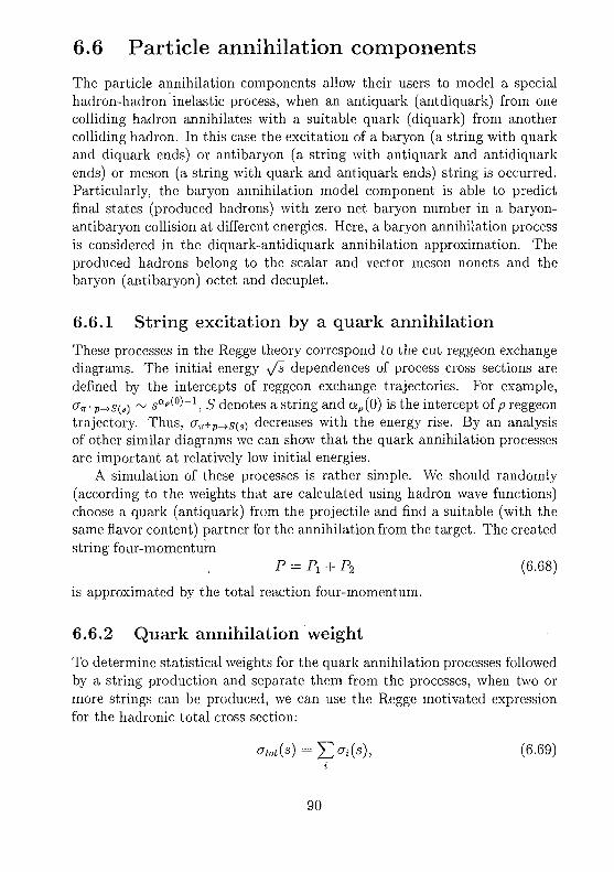
6.6 Particle annihilation components

The particle annihilation components allow their users to model a specialhadron-hadron inelastic process, when an antiquark (antdiquark) from onecolliding hadron annihilates with a suitable quark (diquark) from anothercolliding hadron. In this case the excitation of a baryon (a string with quarkand diquark ends) or antibaryon (a string with antiquark and antidiquarkends) or meson (a string with quark and antiquark ends) string is occurred.Particularly, the baryon annihilation model component is able to predictfinal states (produced hadrons) with zero net baryon number in a baryon-antibaryon collision at different energies. Here, a baryon annihilation processis considered in the diquark-antidiquark annihilation approximation. Theproduced hadrons belong to the scalar and vector meson nonets and thebaryon (antibaryon) octet and decuplet.

6.6.1 String excitation by a quark annihilation

These processes in the Regge theory correspond to the cut reggeon exchangediagrams. The initial energy yfs dependences of process cross sections aredefined by the intercepts of reggeon exchange trajectories. For example,<7TT+P->S(S) ~ s"^0)"1, S denotes a string and 0 ,(0) is the intercept of p reggeontrajectory. Thus, o1T+v^s(s) decreases with the energy rise. By an analysisof other similar diagrams we can show that the quark annihilation processesare important at relatively low initial energies.

A simulation of these processes is rather simple. We should randomly(according to the weights that are calculated using hadron wave functions)choose a quark (antiquark) from the projectile and find a suitable (with thesame flavor content) partner for the annihilation from the target. The createdstring four-momentum

p = P1 + P2 (6.68)

is approximated by the total reaction four-momentum.

6.6.2 Quark annihilation weight

To determine statistical weights for the quark annihilation processes followedby a string production and separate them from the processes, when two ormore strings can be produced, we can use the Regge motivated expressionfor the hadronic total cross section:

= £°i(a)> (6-69)

90

where (7j(s) is the cross section of i-th subprocess. It can be either the elasticcross section <Jei{s) or annihilation cross section with one string productionas(s) or single diffraction cross section OD{S) or multi-string production crosssection CTMS(S)-

From experimental knowledge of the vtotal and elastic cross sections wecan calculate the inelastic cross section:

<?in{s) - crtot{s) - oel(s) = as{s) + aD(s) + aMs(s). (6.70)

The diffraction and multi-string cross sections are calculated according tothe Regge eikonal model as it was described above in the chapter devotedto the hadronic cross sections. Thus, the statistical weight for the quarkannihilation process can be calculated as follows

Ws(s) = (s) - <rD(s)-aMS(s) ^

6.6.3 Baryon annihilation weight

The baryon annihilation cross section aann{s) is used to determine statisticalweights for the diquark annihilation process:

Wann(s) = 4 , (6.72)O'tot(S)

where atot(s) is the total baryon-antibaryon interaction cross section as afunction of the total cm. energy squared.

The baryon annihilation model can be improved by adding another com-peting sub-processes like the string junction annihilation, when three mesonstrings can be produced (see papers [1], [2]).

91

Bibliography

[1] Volkovitskii P. E., Sov. J. Nucl. Phys. 44 729 (1986).

[2] Amelin N. S., Bravina L. V., Sarycheva L. I., Sov. J. Nucl. Phys. 501705 (1989).

92

6.7 Particle inelastic collision components

Here we describe a composite model component that is referred as the Reggeonbased Parton String Model (RPSM). This model is devoted to predict hadron-hadron collisions at high energies. It is originated from the approaches de-scribed in papers [1], [2], [3]. The hadrons that produced in the coursecollisions belong to the scalar and vector meson nonets and the baryon (an-tibaryon) octet and decuplet.

The model can be applied to describe photon-nucleon inelastic collisions.The allowed bombarding energy in hadron-nucleon and photon-nucleon

collisions should be above 2-pions production threshold.This model can also be used to predict elastic and annihilation hadron-

nucleon collisions described in the previous sections.

6.7.1 Particle inelastic collision algorithmThe RPSM algorithm includes a set of the steps should be performed:

• Create projectile and target particles: assign the initial projectile andtarget particle types, their coordinates in the impact parameter spaceand momenta.

• Sample a type of the collision: an elastic, annihilation or inelastic.

• In the cases of elastic and annihilation collisions they are modelled asit was described in the corresponding sections.

• In the case of an inelastic collision sample an impact parameter anddefine a type of the inelastic collision(a diffractive or non-diffractive).Store the total 4-momentum of the collision participants.

• For the non-diffractive inelastic collisions sample a number of longitu-dinal and kinky strings can be produced.

• Perform the longitudinal and kinky string excitations.

• Perform the simulation of string decays (see string decay componentsection).

• Correct energies and momenta of produced particles (see utility com-ponent section), if it is necessary.

93

6.7.2 Sampling of the longitudinal stringsFor an each pair of hadrons i and j with the chosen impact parameters 6j andbj and total cm. energy squared s one should check whether they interactinelastically or not using the probability:

pV?$ - bj,s) = pij(bi - bj, s) + 4 ( £ - bj, s). (6.73)

If the interaction will take place, then one has to decide that it is diffractiveor nondiffractive with the probabilities:

J-^ £-!- (6.74)

and

^44 (6-75)

In the Regge-Gribov approach [4] the probability to find n cut Pomerons[5] or probability for In strings produced in an inelastic collision of the nu-cleons is given by

- bt,s) = cêxP{-2u(bls)}[2u{bl's)]. (6.76)

It is assumed that two strings substitute an each cut Pomeron. By summingof the p\]\h — bj, s) we obtain the non-diffractive probability:

oo

Pijfa - bj,s) = 2 > & W - bf,s). (6.77)7 1 = 1

This probability and other hadron interaction probabilities are defined interms of the amplitude (eikonal) for the nucleon-nucleon elastic scatteringwith Pomeron exchange u(bjj,s). The so-called shower enhancement coeffi-cient c is introduced to determine a contribution of the diffractive dissociation[4] (see hadron cross section section).

6.7.3 Sampling of the kinky stringsTo estimate the number of kinky strings produced in hard hadron collisionswe assume [6], [7] that each cut Pomeron can be substituted either by thetwo longitudinal strings as result of soft hadron interaction or by the twokinky strings as result of hard hadron interactions.

94

At the moment it is not completely clear how to make definite choicebetween the longitudinal and kinky strings to substitute cut Pomerons. Onerecipe is based on the eikonal model [8], [7], where we sum the soft and hardeikonal parts:

u{b%,s) = usoft(bl, s) + uhard(b%,s). (6.78)

The soft eikonal part is defined as

l, s) = - M ^ ( s / S o ) A w * exp[-^./4A.o/t(s)]. (6.79)

The hard part is calculated according to

°it rd(S)}. (6.80)

The ffjet = 0.027 mb and Akard — 0.47 have been found [8] from the fit ofthe two-jets experimental cross section [9]. Then from the global fit of thetotal and elastic cross sections for pp collisions the values of jSOft — 35.5 mb,&sojt = 0.07 and R2

hard = R2soft = 3.56 GeV"2 have been found.

Thus, we can examine each cut Pomeron and substitute it by two kinkystrings with the probability

}?3

6.7.4 Longitudinal string excitation

Let us consider a collision of two hadrons with their c. m. momenta P\ ={Ei , m?/.Ei",0} and P2 = {E% ,m\/E2,0}, where the light-cone variables

E^2 = -Ei,2 i-Pzi,2 are defined through hadron energies £^2 = \frn'i,2 + -f?i,2>hadron longitudinal momenta Pzi i2 and hadron masses mi |2, respectively. Weassume that two hadrons collide by means of two partons with the momentap1 = {x+Ei,0,0} and p2 = {0,x~E2,0}, respectively.

DifFractive string excitation

In the diffractive string excitation (Fritiof approach [10]) only momentumcan be transferred:

P{ = Pi + qPi = P2 - q,

whereQ - {-q2

tl{x-E2-lq2tl{x+Et),<lt} (6.83)

is parton momentum transferred and qt is its transverse component.

95

String excitation by a parton exchange

For this case (the QGSM approach [1]) the parton exchange (rearrangement)and momentum exchange are allowed [1],[2],[3]:

where q = {0,0, q t} is parton momentum transferred.

Transversal and longitudinal momenta generation

The transverse component of a parton momentum transferred is sampledaccording to the probability

P(c[t)dcit = \— exp (—aq,)dqt, (6.85)V n

where the parameter a = 0.6 GeV~2.The light cone parton quantities x+ and x~ are generated independently

and according to the distribution:

u(x) ~xa{l-xY, (6.86)

where x — x+ > xTO,n or x = x~ > xmin. The parameters a — — 1 and13 = 0 are chosen for the FRITIOF approach [10]. In the case of the QGSMapproach [1] the parameters a and /? are explained below. Masses of theexcited strings should satisfy the kinematics constraints:

>mll + ql (6.87)

andP?K > <2 + il (6-88)

where the hadronic masses rrihi and m^ are defined by string quark contents.Thus, a random selection of the values x+ and x~ is limited by the aboveconstraints.

Parton exchange and hadron structure functions

In the QGSM approach [3] strings (as result of a parton rearrangement)should be spanned not only between valence quarks of the colliding hadrons,but also between valence and sea quarks and between sea quarks. Each par-ticipating hadron should be split into a set of partons: valence quark andantiquark for meson or valence quark (antiquark) and diquark (antidiquark)

96

for baryon (antibaryon) as it was explained in the particle structure compo-nent section, and, additionally, into (n — 1) sea quark-antiquark pairs (theirflavours are selected according to the probability ratios u : d : s — 1 : 1 :0.35), if a hadron is participating in n inelastic collisions. As an option thepossibility to split a hadron into sea diquark-antidiquark pairs is included.Such assumption enhances the antibaryon production in the central rapidityregion.

Thus, for each participating hadron we have to generate a set of thelight cone variables X2n, where X2n = x\n or X2n = ^2n according to thedistribution:

2n 2n

fk(xl,X2, ...,X2n) = /o I K f o W l - £**). (6-89)2=1 j = l

where /o is a normalization constant. In the last expression u^. (xt) denotethe hadron structure functions for valence quark (antiquark) qv, sea quarkand antiquark qs and valence diquark (antidiquark) qq:

<(xv) = x?, <(xs) = x?, uhqq{xqq) = xfc, (6.90)

where av = —0.5 and as = -0.5 [1] for the non-strange quarks (antiquarks)and av = 0 and as — 0 for strange quarks (antiquarks), puu — 1.5 and(5ud = 2.5 in the case of proton (antiproton) and (3dct — 1.5 and j3ud = 2.5 in thecase of neutron (antineutron). Usually Xj is selected between xfm < X{ < 1,where the model parameter xmm = 0.3/y^ is a function of initial energy i/s.It prevents the production of strings with low masses (smaller than hadronmasses), while the whole selection procedure should be repeated.

The transversal momenta of partons qit are generated according to theGaussian probability Eq. (6.85) with a — l/4A(s), where X(s) is calculatedaccording to the Eq. (6.15), and under the constraint: XîQit = 0. Thus,the partons are considered as the off-shell or virtual partons.

6.7.5 Kinky string excitation

Having sampled configuration of the kinky strings we perform kinky stringexcitations.

It is performed by means of two steps for each pair of kinky strings.At first step we determine the total 4-momentum of each kinky string fromthe chosen pair. Then we generate 4-momentuma of the gluon-kinks. Thefirst step is fulfilled in the same way as it was described for a pair of thelongitudinal strings. To fulfill the second step we assume that kinky stringsare produced as the result of gg —>• gg hard interactions. Our consideration

97

of the outgoing gluons (kinks) momenta is based on the two-jets inclusiveproduction cross section:

where we take s = Q2 = x£x~s and 5 is the total center of mass energysquared for the colliding system that is calculated using x; and qti and mf ofthe string end partons. The value of s should be large enough to producegluons with the transverse momentum above the chosen cutoff Ql = 2 GeV2.f(x,Q2) is the momentum fraction distribution of gluons in the hadron. Itcan be chosen from [11]. The QCD gluon-gluon interaction cross sectionJ"s ^, where 9 is the scattering angle in the center of mass of the parton-

parton system and it was calculated in the Born approximation [12]. Simula-tion of an elastic gluon-gluon scattering is described in the elastic scatteringcomponents section.

Thus, the MC procedure to build kinky strings can be outlined as follows:

• Sample Xi, qit and m|, where i = 1,2, ...,2n, for the partons, whichwill be on the In string ends for both soft and kinky strings.

• For each pair of the kinky strings calculate the total center of massenergy s and sample x+ > x+in and x~ > xîn, where xmin = 2Q0/\/s,using the gluon distribution.

• Sample the center of mass scattering angle 9 for outgoing gluons andcalculate their 4-momenta.

• For each kinky string recalculate the energies and momenta of partonstring ends.

This procedure should be improved taking into account gluon radiation.

Bibliography

[1] Kaidalov A. B., Ter-Martirosyan K. A., Phys. Lett. B117 247 (1982).

[2] Capella A., Sukhatme U., Tan C. I., Tran Thanh Van. J., Phys. Rep.236 225 (1994).

[3] Amelin N. S., Bravina L. B., Sov. J. Nucl. Phys. 51 221 (1990).

[4] Baker M. and Ter-Martirosyan K. A., Phys. Rep. 28C 1 (1976).

[5] Abramovskii V. A., Gribov V. N., Kancheli O. V., Sov. J. Nucl. Phys.18 308 (1974).

[6] Amelin N. S., Stocker H, Greiner W., Armesto N., Braun M. A., PajaresC., Phys. Rev. C52 362 (1995).

[7] Werner K., Drescher H. J., Furler E., Hladik M., Ostapchenko S., inProc: 3rd Inter. Conf. on Physics and Astrophysiks of Quark-GluonPlasma, Jaipur, India, March 17-21, 1997.

[8] Ranft J, Capella A., Tran Thanh Van, Phys. Lett. B320 346 (1994).

[9] UA1 Collab., Albajar C. et al, Preprint CERN-EP/88-29.

[10] Andersson B., Gustafson G., Nielsson-Almquist, Nucl. Phys. 281 289(1987).

[11] Capella A., Kaidalov A., Merino C, Tran Thanh Van J., Phys. Lett.B343 403 (1995).

[12] Combrige B. L. , Kripfganz J. , Ranft J. , Phys. Lett. 70B 234 (1977);Cutler R., Sivers D., Phys. Rev. D17 196 (1978).

99

6.8 Nuclear model components

6.8.1 Nuclear properties

We have tabulated the experimental values [1] of nuclear masses and bindingenergies. There is a possibility to calculate nuclear masses as well as bindingenergies applying the liquid drop model formulas.

Bethe-Weizsacker's formula

In this approach [2] the nucleus binding energy B(A, Z) is given by the sumof volume, surface and Coulomb energy terms, respectively:

B{A,Z) =

= -0.01587A + 0.01834A2/3 + 0.09286 (z - ^ + 0.00071-^, ^'92'

where A is the number of nuclear nucleons and Z is the number of nuclearprotons.

Nucleon potential

For i-th nucleon with radius r* this potential is defined by a sum of theFermi-potential

Tf\n) = & ^ , (6.93)

binding energy B(A, Z) and Coulomb (for protons only) potential Vc{Z,ri):

V(A, Z, n) = TF(n) + B(A, Z) + VC(Z, n). (6.94)

The Fermi-momentum in the local Thomas-Fermi approximation [3] de-pends on proton or neutron density PZ,N{T) as follows

pF(r) = h{Zv2pz>Nyi\ (6.95)

were h = 197.327 MeVfm.The Coulomb barrier (in MeV) is given by

( 6" 9 6 )

where C = 1.44 MeVfm and r0 = 1.3 fm.

100

6.8.2 Nucleus initial state simulationThe initialization of colliding nucleus, consisting of A nucleons and Z protons(N = A — Z neutrons) with coordinates rt- and momenta p,, where i —1,2,..., A, should be performed in the case of nuclear collision simulation bydifferent models (see, e.g., the inelastic nuclear collision component section).

The MC initialization procedure can be outlined as follows:

1. Nucleon radii ri are selected randomly at the rest of nucleus accordingto proton or neutron density pin). The normalized nucleon density forheavy nuclei with A > 16 [4] is

HVtl l + expKn-R)/^

where—1

Here R = r0A^3 fm and r0 = 1.16(1 - 1.16A~2/3) fm and a « 0.545fm. The normalized density of light nuclei with A < 17 is given by theharmonic oscillator shell model [5], i. e.,

pin) - (nR2y3/2 exp (-r2/R2), (6.99)

where R2 = 2/3 < r2 >= 0.8133.42/3 fm2 or

where

Q Y' (< >A - < r\ >p). (6.101)The mean charge radii squared for nucleus < r2

h >& and proton <rch >P a r e taken from the lepton-nucleus scattering experiments [6]. Totake into account the nucleon repulsive core it is assumed that inter-nucleon distance d > 0.8 fm;

2. The nuclear radius with counting of diffuseness is determined from thecondition:

g | (6.102)

3. The momenta of the nucleons are randomly chosen between 0 andPmaxir) with equal probabilities, where Pmax(r) 1S calculated accord-ing to the Eq. (6.95).

101

4. To obtain coordinate and momentum vector components, it is assumedthat nucleons are distributed isotropically in the configuration and mo-mentum spaces;

5. The nucleus must be centered in configuration space around 0, i. e.Yliî = 0 and it must be at rest, i. e., S i Pi = 0 and S i r i x p; = 0.To provide the first two conditions we can perform shifts of nucleoncoordinates v[ = r*i — I/A J2i r i ar>d momenta p[ — p; — I/A £}» p;.

6. There is a possibility to unpack a nucleus into free streaming nucleonshaving effective masses by computing the energy per nucleon as e —E/A — mjv + B(A,Z)/A, where m# is the nucleon mass and nucleusbinding energy B(A,Z) given by the Bethe-Weizsacker formula (Eq.(6.92)), and assigning the effective mass ntf = \J{E/A)2 — pf foreach nucleon.

102

Bibliography

[1] Audi G., Wapstra A. H., Nucl. Phys. A595 V. 4 409 (1995).

[2] Bohr A., Mottelson B. R., Nuclear Structure, W. A. Benjamin, NewYork, Vol. 1, 1969.

[3] DeShalit A., Feshbach H., Theoretical Nuclear Physics, Vol. 1: NuclearStructure, Wyley, 1974.

[4] Grypeos M. E., Lalazissis G. A., Massen S. E., Panos C. P., J. Phys.G17 1093 (1991).

[5] Elton L. R. B., Nuclear Sizes, Oxford University Press, Oxford, 1961.

[6] Barrett R. C. and Jackson D. F., Nuclear Sizes and Structure. OxfordUniversity, New York, 1977.

103

6.9 Inelastic nuclear collision components

Here we describe a composite model component that is referred as the Pomeronbased Parton String Model (PPSM). This model is devoted to predict in-elastic collisions of a large variety of hadron (the same types as final statehadrons) and nuclear projectiles with nucleon and nuclear targets. Theproduced hadrons belong to the scalar and vector meson nonets and thebaryon (antibaryon) octet and decuplet. The allowed bombarding energiesin a hadron-nucleon collision should be above 2-pions production threshold.In the case of hadron-nucleus or nucleus-nucleus collisions the initial energies•>/s > 5 AGeV are recommended. This model is also able to predict finalstates (produced hadrons) in photon-nucleon and photon-nucleus inelasticcollisions at the initial energies y/s > 5 AGeV.

6.9.1 Nuclear inelastic collision algorithm

The PPSM algorithm includes a following set of the steps should be per-formed:

» Create two vectors (a projectile and target) of particles. Assign theinitial projectile and target particle types, their coordinates and mo-menta. In the case of a hadron-nucleus (or nucleus-nucleus) interactionone should perform the target nucleus (or projectile and target nuclei)initial state simulation (see the nuclear model component section) andsample an impact parameter;

» Sample collision participants and separated them into a diffractive andnon-diffractive. Store the total interaction four momentum for theparticipants;

• For each non-diffractive inelastic collisions sample the numbers of lon-gitudinal and kinky string can be produced;

• Excite and re-excite colliding particles in the case of diffractive col-lisions and create diffractive longitudinal strings, if particles are notparticipate in the further soft or hard collisions;

• Perform the longitudinal and kinky string excitations;

• Perform the simulation of string decays (see the string decay componentsection);

• Correct energies and momenta of produced particles (see the utilitycomponents section), if it is necessary.

104

6.9.2 Initial state simulation

An impact parameter value (0 < b < Rp + Rt) is randomly selected accordingto the distribution:

P(b) = b. • (6.103)

Then one should update the transversal components of projectile coordinates:

rxi -» rxi + bx (6.104)

andryi -+ ryi + by. (6.105)

For the target nucleus, if a projectile is centered on the origin of coordinatesystem, one should perform a shift of nucleon longitudinal coordinates:

TZi —>• rzi + Arz/ji, (6.106)

where Arz = Rp + 1.5 fm + Rt + 1.5 fm can be taken.The chosen working frames, where an interaction process is simulated,

are the c. m. frame of colliding particles and particle equal velocities frame,respectively, in the case of particle and nuclear interactions.

In the case of a fast moving nucleus with the initial momentum per nu-cleon P o = {0,0, PZQ} one should perform Lorentz transformation of thenucleon longitudinal momenta

Pzi -> 7i(Pzi ~ AeO (6.107)

and the nucleon energies

ei ->• 7i(e, - PiPzi), (6.108)

where /?; is denned as

A = 2P z 0

gff2 (6.109)

and 7$ is given by

•"^nt (6-no>

The ml ' denotes an effective i-th nucleon mass.For a fast moving nucleus one needs also to perform its Lorentz contrac-

tion, i. e.,ri = r, - - f - v ( v r i ) , (6.111)

105

where v is the nuclear velocity and 7 — 1/Vl — v2. The nucleus initializationcan be performed at once, even if one needs to simulate multiple nuclearinteractions, when the same nucleus is participating. The nucleus is randomlyrotated in coordinate and momentum spaces before repeated interaction. Toperform this rotation three Euler angles: 0 < 81 < 2ir, 0 < 82 < 2TT and0 < #3 < 2n are selected (with the uniform probabilities) randomly. Thenthe nucleon coordinates r; = {rare rotated sequentially:

r ;

and

xi,ryi,rzi} and momenta p ; = {pxi,pyi,Pzi}

(6.112)

(6.113)Pi — Pi^M —y Pi-^2 — Pi^sJi

where the rotation matrices are determined as follows

cos #! - sin 9\ 0sin 9\ cos 8\ 0

0 0 1

and

and

R2 =cos 82 0 — sin 82

0 1 0sin 82 0 cos 82

cos #3 - sin #3 0sin 9s cos #3 0

0 0 1

(6.114)

(6.115)

(6.116)

6.9.3 Nuclear collision participants

The ultra-relativistic inelastic hadron-nucleus and nucleus-nucleus collisionsare considered as independent hadron-nucleon and nucleon-nucleon inelasticcollisions. It was shown long time ago [1] for the hadron-nucleus collision thatsuch picture can be obtained starting from the Regge-Gribov approach [2],where the hadron-nucleus elastic scattering amplitude is a result of reggeonexchanges between initial hadron and nucleons from a target-nucleus. Thisresult can be extended for the nucleus-nucleus collision case and leads toa simple and efficient MC procedure [3] to define interaction cross sectionsand number of the nucleons participating in the inelastic nucleus-nucleuscollision:

106

1. We randomly distribute A nucleons from the projectile-nucleus and Bnucleons from the target-nucleus inside the impact parameter plane ac-cording to the weight functions T([bf ]) and T([bf]), respectively. These .functions represent probability densities to find sets of nucleon impactparameters [bf] and [bf], where i — 1,2,...,A and j = 1,2,..., 5 , re-spectively.

2. For each pair of nucleons i and j with chosen impact parameters bf andbf we check whether they interact inelastic or not using the probabilityPij{bf — bf,s), where sy- = (p; +Pj)2 is the total cm. energy squaredof the given nucleons with the 4-momenta p, and pj, respectively.

The described MC procedure is based on the probability P(B, s) of a suchconfiguration, when several pairs of nucleons from the projectile and targetnuclei interact inelastically and the rest of the nucleons do not participate incollisions:

P(B, *) = ( II Pv(% - bf, s) II [1 - rf - %,s)}\ , (6.117)\i,j=l k,l=l I

where B is an impact parameter for the colliding nuclei and s is total cm.nucleon-nucleon energy squared. To simplify notations, we assume, that allinteracting nucleon pairs have the same s. The last equation can be rewrittenmore explicitly as follows

P(B, s) = J n ViSt - bf, s) n [1 - P J U $ - bf, s)]xM = I *>i=i (6.118)

xTA(b?)TA(b£)...TA(B - b*)dUtdbB

The probability for an inelastic collision of the nucleons i and j as afunction of the squared impact parameter difference &?• = (bf — b^)2 and 5can be calculated within the Regge-Gribov approach [4], [2] (see the hadroncross section section).

We would stress that in the Pomeron eikonal model [2] we count onlyPomeron exchanges for the hadron elastic scattering amplitude. With suchamplitude we are not able to predict properly the experimental values ofhadron interaction cross sections and also the corresponding interaction prob-abilities in the whole energy range under consideration. We will stronglyunderestimate low energy parts of the cross sections and the correspondinginteraction probabilities.

At this energy region neglecting by the real part of a hadron scatteringamplitude we can correct the eikonal variables (see the hadron cross section

107

section) expressing them through experimental values of the total atot(s),elastic aei{s) and single diffraction a^(s) cross sections:

\{s) = 2^(3) , (6.120)

whereT> f \ tot\ I (n -t cy-\ \

elK >~ 87r[<jel(s)+ ad{s)Y K • '

108

Bibliography

[1] Capella A. and Krzywicki A., Phys. Rev. D18 (1978) 4120.

[2] Baker M. and Ter-Martirosyan K. A., Phys. Rep. 28C (1976) 1.

[3] Amelin N. S., Gudima K. K., Toneev V. D., Sov. J. Nucl. Phys. 51(1990) 327; Amelin N. S., JINR Report P2-86-56 (1986).

[4] Abramovskii V. A., Gribov V. N., Kancheli 0 . V., Sov. J. Nucl. Phys.18 (1974) 308.

109

6.10 Utility components

We have developed a set of the components to fulfill utility functions in thecourse of particle and nuclear collisions modeling. As a rule these componentsdeal with particle 4-momenta [1].

6.10.1 Energy-momentum correction

Sometimes we need to correct the energy and momentum of each producedparticle to guarantee the energy-momentum conservation law for a collidingsystem. The correction procedure consists of three steps:

» We boost 4-momenta of the produced particles into their center of massframe using the total velocity of produced particles.

• We scale 3-momentum of each produced particle until their summarymass is close to the effective mass of the colliding system. The scalingprocedure is controlled by a difference of a scale factor from the unit.

• We perform the reverse boost of 4-momenta of the produced particlesinto the initial colliding frame using the velocity of the colliding system.

6.10.2 Particle distributions

As result of a particle or nuclear collision simulation we obtain the values ofparticle 3-momenta (px>Py>Pz) > their energies (E), their quantum numbers,i.e., the particle types. This information allows us a possibility to build differ-ent particle distributions. The particle rapidity y ~ —0.5 In j ^ 2 ^ distributionis calculated according to the equation:

|5 = ££<%*-*/) . (6-122)where n is the mean multiplicity of particles of the required type, Nevt is thenumber of generated collision events, nk is the number of particles of requiredtype in k-th event. Similarly we can build other particle distributions, e.g.,transversal momentum pt distribution:

,/fj 1 Nevt nh

- T7— 2_j 2—i° \Ptj Pt)- {o.iôj

110

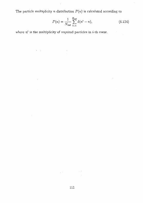
The particle multiplicity n distribution P(n) is calculated according to

where ri1 is the multiplicity of required particles in i-th event.

I l l

Bibliography


Received by Publishing Departmenton August 23, 2001.

112

Амелин Н. С , Комогоров M. Э. Д11-2001-175Компонентно-ориентированный подходк разработке и использованию численных моделейв физике высоких энергий

Обсуждаются основные концепции компонентного подхода к разработкеи применению численных моделей в физике высоких энергий. Данный подходреализован в виде системы программ NiMax. Обсуждаемые концепции иллю-стрируются многочисленными примерами работы пользователя системы.В приложении описаны физика и численные алгоритмы компонентов для мо-делирования событий взаимодействия частиц и ядер при высоких энергиях.Эти компоненты входят в состав прикладных модулей адронных моделей, со-зданных в рамках данной системы. Данное описание может рассматриватьсякак предварительная версия руководства для пользователей моделирующихкомпонентов, работающих с системой NiMax.

Работа выполнена в Лаборатории высоких энергий ОИЯИ.

Сообщение Объединенного института ядерных исследований. Дубна, 2001

Amelin N. S., Komogorov M. E. Dl 1-2001-175Component-Oriented Approach to the Developmentand Use of Numerical Models in High Energy Physics

We discuss the main concepts of a component approach to the developmentand use of numerical models in high energy physics. This approach is realized asthe NiMax software system. The discussed concepts are illustrated by numerousexamples of the system user session. In appendix chapter we describe physicsand numerical algorithms of the model components to perform simulationof hadronic and nuclear collisions at high energies. These components are mem-bers of hadronic application modules that have been developed with the helpof the NiMax system. Given report is served as an early release of the NiMax man-ual in the main for model component users.

The investigation has been performed at the Laboratory of High Energies,JINR.

Communication of the Joint Institute for Nuclear Research. Dubna, 2001

Макет Т. Е. Попеко

ЛР№ 020579 от 23.06.97.Подписано в печать 23.01.2002.

Формат 60 X 90/16. Бумага офсетная. Печать офсетная.Усл. печ. л. 7,0. Уч.-изд. л. 9,78. Тираж 170 экз. Заказ № 53003.

Издательский отдел Объединенного института ядерных исследований141980, г. Дубна, Московская обл., ул. Жолио-Кюри, 6.

Documents

D11-2001-175 N. S. Araelin, M. E. Komogorov

Bibliography

[1] Particle-Data-Group, Phys. Rev. D54 1 (1996).