D. Receiver Dynamic Range

10/29/2007 Receiver Dynamic Range notes 1/1

Jim Stiles The Univ. of Kansas Dept. of EECS

D. Receiver Dynamic Range Q: So can we apply our new knowledge about noise power to a super-het receiver? A: Example: Receiver Gain and Noise Figure Q: What about the input signal power? You said it can be very large or very small. Are there any limits to the signal power? A: Yes! If the signal power is too small, it cannot be accurately demodulated due to signal noise. HO: The Minimum Detectable Signal Likewise, if the signal power is too large, the receiver will saturate! HO: Receiver 1dB Compression Point The ratio of the largest to smallest signal power defines the dynamic range of a receiver. HO: Receiver Dynamic Range

10/29/2007 Example Receiver Gain and Noise Figure 1/5


Example: Receiver Gain and Noise Figure

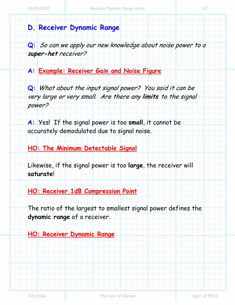
We cam now determine the overall gain and noise figure of a super-het receiver! Consider the following example: Let’s look at each device individually: Antenna - We assume that the antenna noise temperature is

290A oT T K= = , therefore 174AN dBm Hz= − . Also, the antenna couples in a desired signal with power in

sP . 1. LNA - This device has a gain 1 10 0G .= (10 dB) and a noise figure 1 1 5F .= (1.76 dB). 2. Preselector – This device has an insertion loss of 1 dB. Therefore:

1 2 3

4 in

sP outsP

5



( )

( )

2 2

2 2

1 0 0 8

1 0 1 26

G dB . G .

F dB . F .

= − ⇒ =

= ⇒ =

3. Mixer - This device has an conversion loss of 6 dB. Therefore:

( )

( )

3 2

3 2

6 0 0 25

6 0 4 0

G dB . G .

F dB . F .

= − ⇒ =

= ⇒ =

4. IF Amp - This device has a gain 4

310G = (30 dB) and a noise figure 4 4 0F .= (6 dB). 5. IF Filter - This device has an insertion loss of 2 dB. Therefore:

( )

( )

5 2

5 5

2 0 0 63

2 0 1 58

G dB . G .

F dB . F .

= − ⇒ =

= ⇒ =

The total gain of the receiver is easy to determine, its simply the product of the gains of all devices:

( ) ( ) ( ) ( ) ( )1 2 3 54

10 0 8 0 25 1000 0 631260

xRG G G G G G. . .

=

=

=

or,



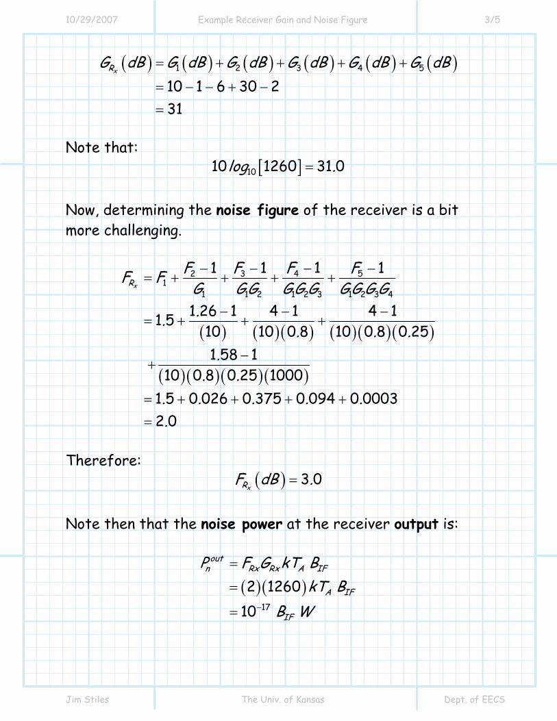
( ) ( ) ( ) ( ) ( ) ( )1 2 3 54

10 1 6 30 231

xRG dB G dB G dB G dB G dB G dB= + + + +

= − − + −

=

Note that:

[ ]1010 1260 31 0log .=

Now, determining the noise figure of the receiver is a bit more challenging.

( ) ( ) ( ) ( ) ( ) ( )

( ) ( ) ( ) ( )

3 4 521

1 1 2 1 2 3 1 2 3 4

11 11

1 26 1 4 1 4 11 510 10 0 8 10 0 8 0 251 58 1

10 0 8 0 25 10001 5 0 026 0 375 0 094 0 00032 0

xRFF FFF F

G GG GG G GG G G..

. . ..

. .. . . . ..

−− −−= + + + +

− − −= + + +

−+

= + + + +

=

Therefore:

( ) 3 0xRF dB .=

Note then that the noise power at the receiver output is:

( ) ( )17

2 126010

outn Rx Rx A IF

A IF

IF

P F G kT BkT B

B W−

=

=

=



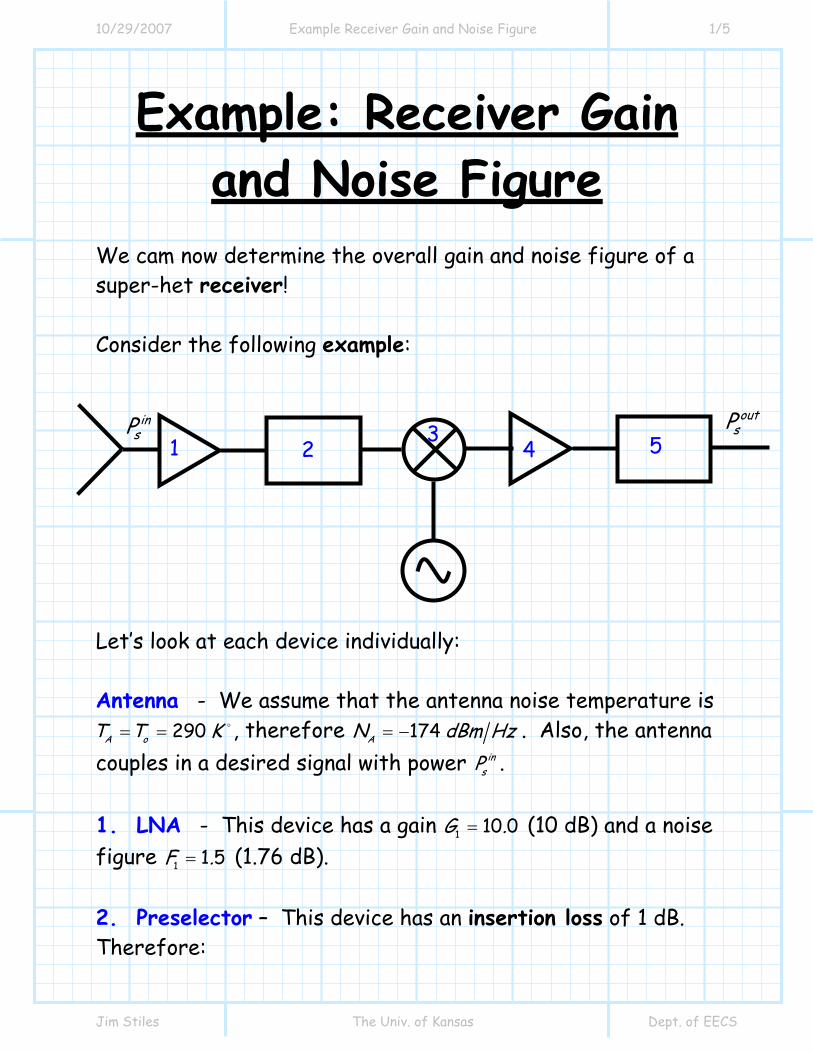
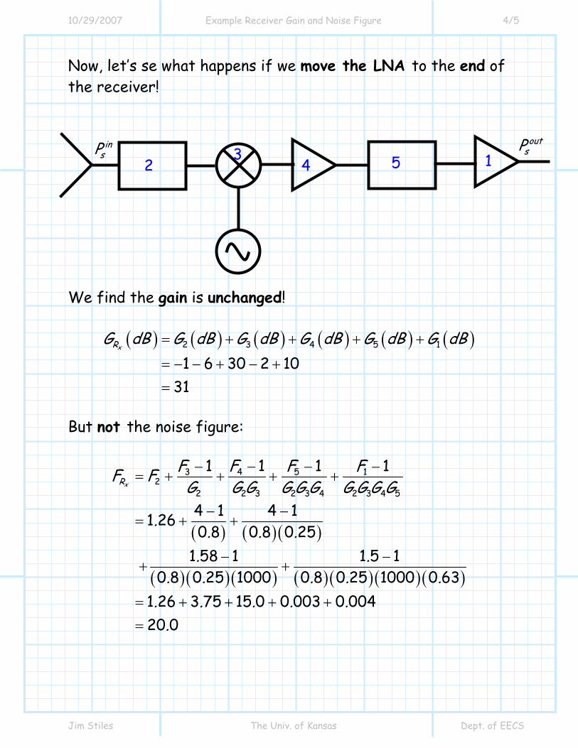
Now, let’s se what happens if we move the LNA to the end of the receiver! We find the gain is unchanged!

( ) ( ) ( ) ( ) ( ) ( )2 3 5 14

1 6 30 2 1031

xRG dB G dB G dB G dB G dB G dB= + + + +

= − − + − +

=

But not the noise figure:

( ) ( ) ( )

( ) ( ) ( ) ( ) ( ) ( ) ( )

3 4 5 12

2 2 3 2 3 2 3 54 4

11 1 1

4 1 4 11 260 8 0 8 0 25

1 58 1 1 5 10 8 0 25 1000 0 8 0 25 1000 0 63

1 26 3 75 15 0 0 003 0 00420 0

xRFF F FF F

G G G G G G G G G G

.. . .

. .. . . . .

. . . . ..

−− − −= + + + +

− −= + +

− −+ +

= + + + +

=

1 2 3

4 in

sP outsP

5



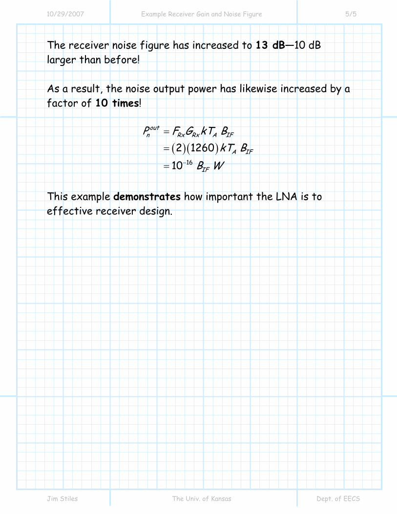
The receiver noise figure has increased to 13 dB—10 dB larger than before! As a result, the noise output power has likewise increased by a factor of 10 times!

( ) ( )16

2 126010

outn Rx Rx A IF

A IF

IF

P F G kT BkT B

B W−

=

=

=

This example demonstrates how important the LNA is to effective receiver design.

10/29/2007 Minimum Detectable Signal 1/6


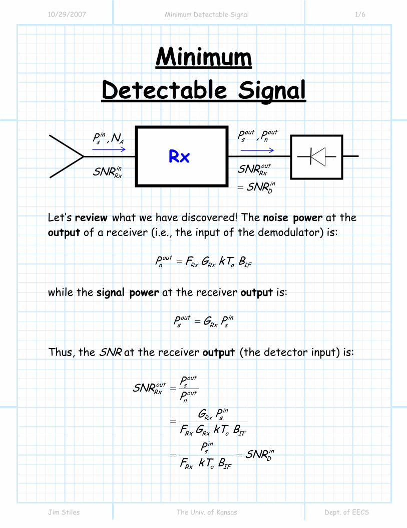
Minimum Detectable Signal

Let’s review what we have discovered! The noise power at the output of a receiver (i.e., the input of the demodulator) is:

outn Rx Rx o IFP F G kT B=

while the signal power at the receiver output is:

out ins Rx sP G P=

Thus, the SNR at the receiver output (the detector input) is:

outout s

Rx outn

inRx s

Rx Rx o IFin

insD

Rx o IF

PSNRP

G PF G kT B

P SNRF kT B

=

=

= =

Rx in

s A

inRx

P ,N

SNR

out outs n

outRx

inD

P ,P

SNRSNR=



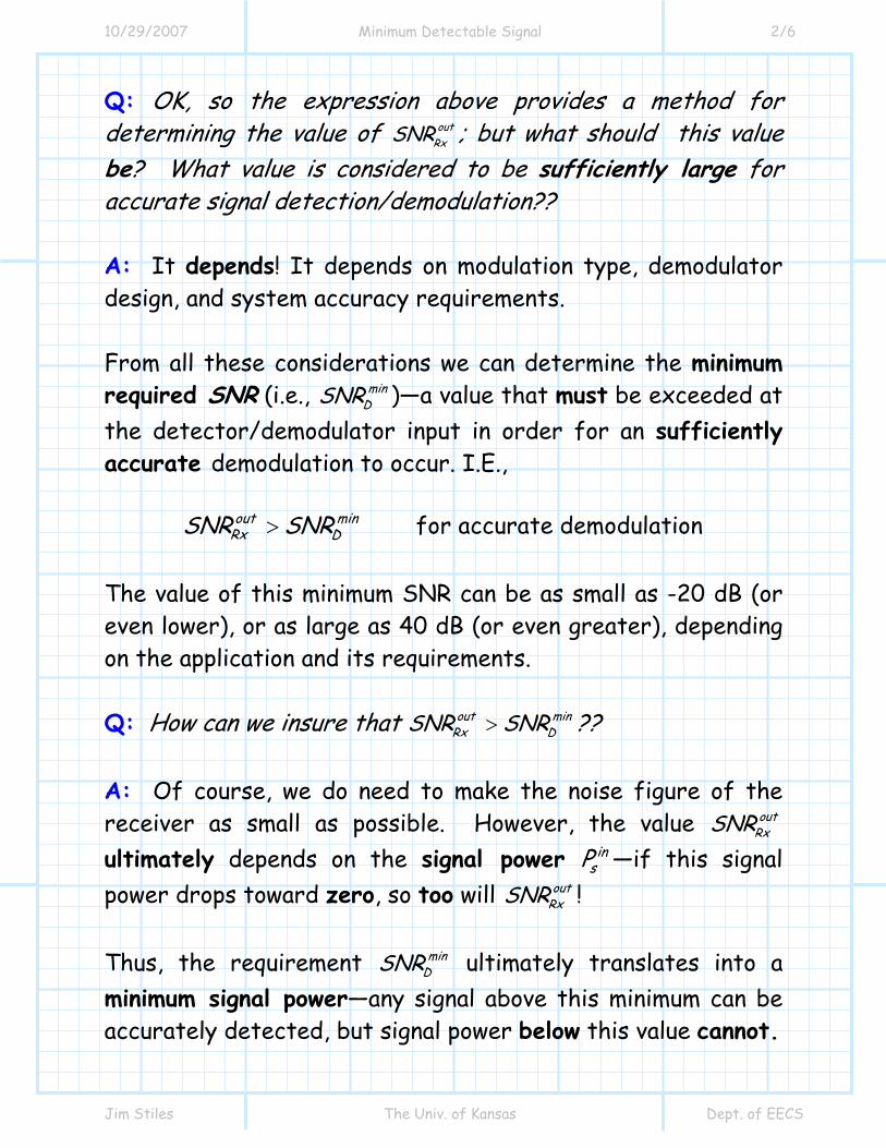
Q: OK, so the expression above provides a method for determining the value of out

RxSNR ; but what should this value be? What value is considered to be sufficiently large for accurate signal detection/demodulation?? A: It depends! It depends on modulation type, demodulator design, and system accuracy requirements. From all these considerations we can determine the minimum required SNR (i.e., min

DSNR )—a value that must be exceeded at the detector/demodulator input in order for an sufficiently accurate demodulation to occur. I.E.,

for accurate demodulationout minRx DSNR SNR>

The value of this minimum SNR can be as small as -20 dB (or even lower), or as large as 40 dB (or even greater), depending on the application and its requirements. Q: How can we insure that out min

Rx DSNR SNR> ?? A: Of course, we do need to make the noise figure of the receiver as small as possible. However, the value out

RxSNR ultimately depends on the signal power in

sP —if this signal power drops toward zero, so too will out

RxSNR ! Thus, the requirement min

DSNR ultimately translates into a minimum signal power—any signal above this minimum can be accurately detected, but signal power below this value cannot.



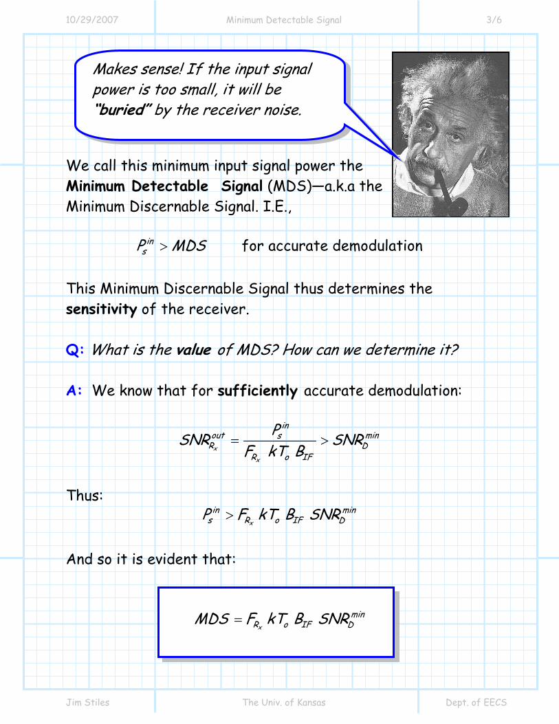
We call this minimum input signal power the Minimum Detectable Signal (MDS)—a.k.a the Minimum Discernable Signal. I.E.,

for accurate demodulationinsP MDS>

This Minimum Discernable Signal thus determines the sensitivity of the receiver. Q: What is the value of MDS? How can we determine it? A: We know that for sufficiently accurate demodulation:

x

x

inout mins

R DR o IF

PSNR SNRF kT B

= >

Thus:

x

in mins R o IF DP F kT B SNR>

And so it is evident that:

x

minR o IF DMDS F kT B SNR=

Makes sense! If the input signal power is too small, it will be “buried” by the receiver noise.



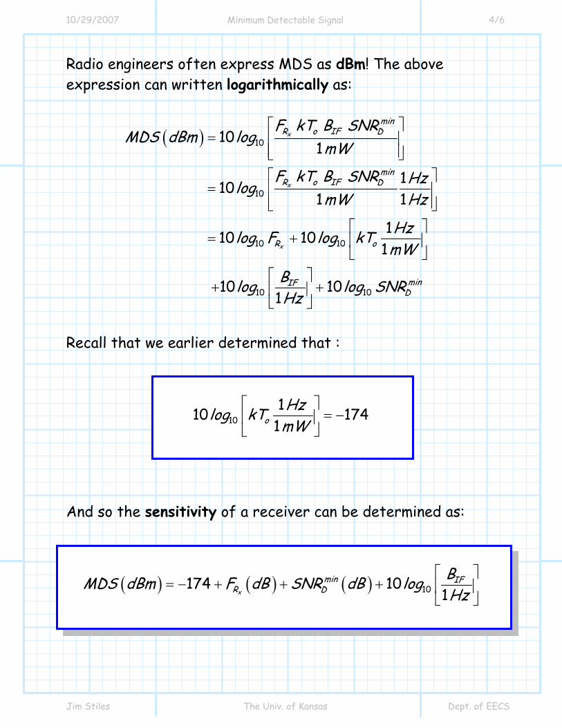
Radio engineers often express MDS as dBm! The above expression can written logarithmically as:

( ) 10

10

10 10

10 10

101

1101 1

110 101

10 101

x

x

x

minR o IF D

minR o IF D

R o

minIFD

F kT B SNRMDS dBm log

mW

F kT B SNR HzlogmW Hz

Hzlog F log kTmW

Blog log SNRHz

⎡ ⎤= ⎢ ⎥

⎢ ⎥⎣ ⎦⎡ ⎤

= ⎢ ⎥⎢ ⎥⎣ ⎦

⎡ ⎤= + ⎢ ⎥

⎣ ⎦⎡ ⎤

+ +⎢ ⎥⎣ ⎦

Recall that we earlier determined that :

10110 174

1oHzlog kTmW

⎡ ⎤= −⎢ ⎥

⎣ ⎦

And so the sensitivity of a receiver can be determined as:

( ) ( ) ( ) 10174 101x

min IFR D

BMDS dBm F dB SNR dB logHz

⎡ ⎤= − + + + ⎢ ⎥

⎣ ⎦



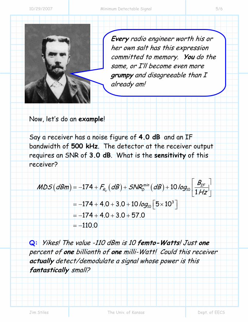
Now, let’s do an example! Say a receiver has a noise figure of 4.0 dB and an IF bandwidth of 500 kHz. The detector at the receiver output requires an SNR of 3.0 dB. What is the sensitivity of this receiver?

( ) ( ) ( ) 10

310

174 101

174 4 0 3 0 10 5 10174 4 0 3 0 57 0110 0

x

min IFR D

BMDS dBm F dB SNR dB logHz

. . log

. . ..

⎡ ⎤= − + + + ⎢ ⎥

⎣ ⎦⎡ ⎤= − + + + ×⎣ ⎦

= − + + +

= −

Q: Yikes! The value -110 dBm is 10 femto-Watts! Just one percent of one billionth of one milli-Watt! Could this receiver actually detect/demodulate a signal whose power is this fantastically small?

Every radio engineer worth his or her own salt has this expression committed to memory. You do the same, or I’ll become even more grumpy and disagreeable than I already am!



A: You bet! The values used in this example are fairly typical, and thus an MDS of -110 dBm is hardly unusual. It’s a good thing too, as the signals delivered to the receiver by the antenna are frequently this tiny!

10/29/2007 Receiver Compression Point 1/14


Receiver Saturation Point

Given the gain RxG of a receiver, we know that the output signal power (i.e., the signal power at the demodulator) is:

in out ins Rx sDP P G P= =

Of course, in

sP can theoretically be any value; but outsP is

limited! Q: Limited by what? A: Many of the devices in a receiver have compression points (e.g., mixers and amplifiers)! In other words, as in

sP increases, one of the devices in the receiver will eventually compress (i.e., saturate). As we increase the signal power in

sP beyond this point, we find that the receiver output power will be less than the value in

Rx sG P .

Precisely the same behavior as an amplifier or mixer! Accordingly, we can define a 1dB compression point for our receiver.



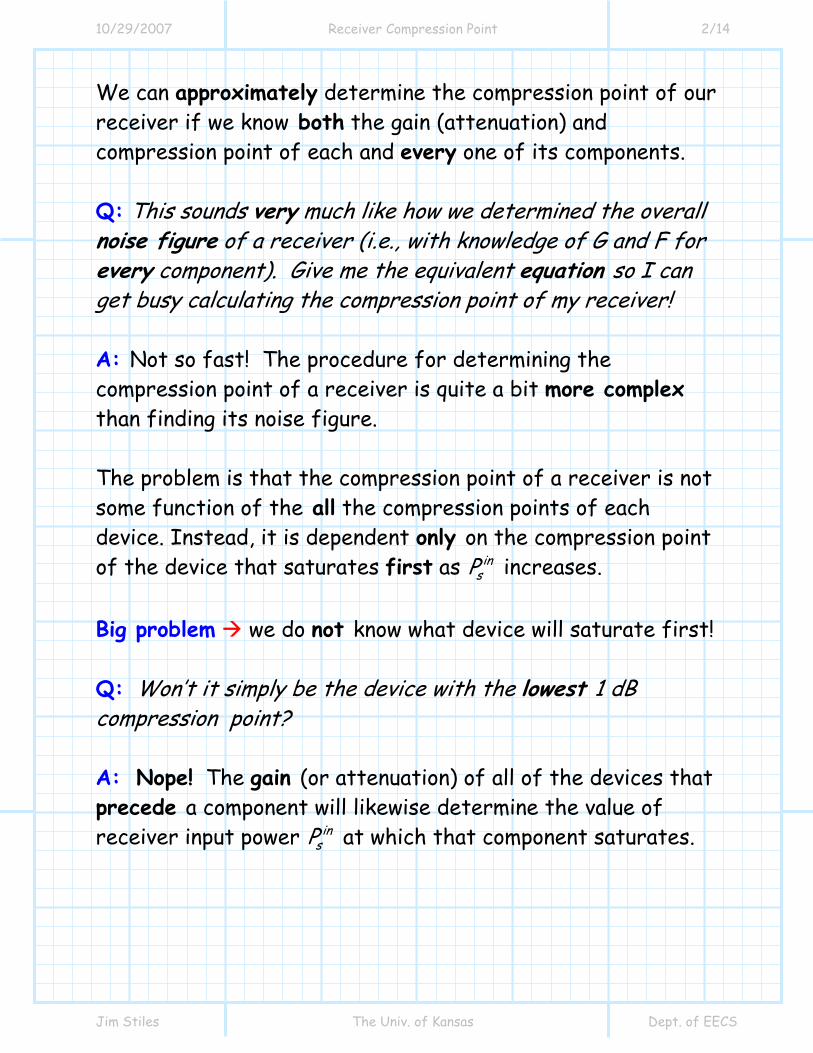
We can approximately determine the compression point of our receiver if we know both the gain (attenuation) and compression point of each and every one of its components. Q: This sounds very much like how we determined the overall noise figure of a receiver (i.e., with knowledge of G and F for every component). Give me the equivalent equation so I can get busy calculating the compression point of my receiver! A: Not so fast! The procedure for determining the compression point of a receiver is quite a bit more complex than finding its noise figure. The problem is that the compression point of a receiver is not some function of the all the compression points of each device. Instead, it is dependent only on the compression point of the device that saturates first as in

sP increases. Big problem we do not know what device will saturate first! Q: Won’t it simply be the device with the lowest 1 dB compression point? A: Nope! The gain (or attenuation) of all of the devices that precede a component will likewise determine the value of receiver input power in

sP at which that component saturates.



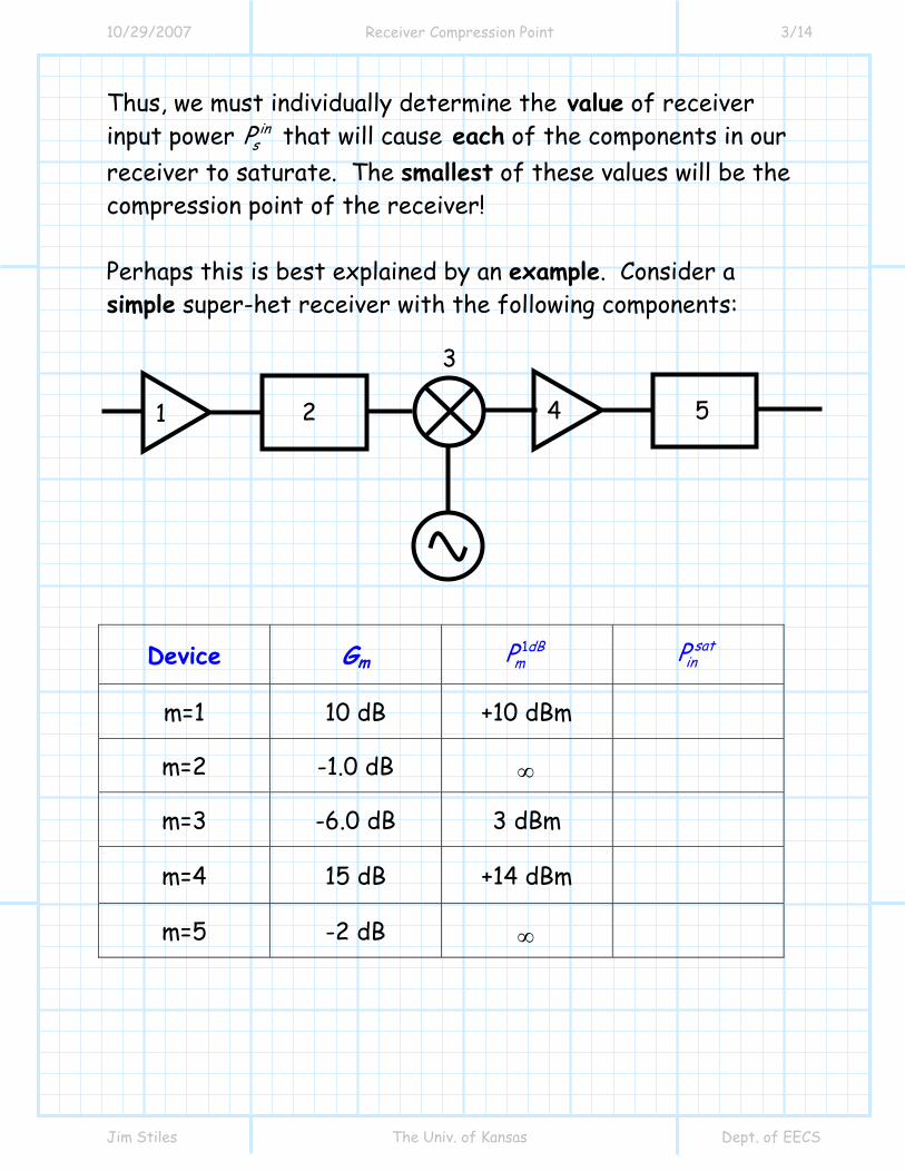
Thus, we must individually determine the value of receiver input power in

sP that will cause each of the components in our receiver to saturate. The smallest of these values will be the compression point of the receiver! Perhaps this is best explained by an example. Consider a simple super-het receiver with the following components:

Device Gm 1dBmP sat

inP

m=1 10 dB +10 dBm

m=2 -1.0 dB ∞

m=3 -6.0 dB 3 dBm

m=4 15 dB +14 dBm

m=5 -2 dB ∞

1 2

3

4 5



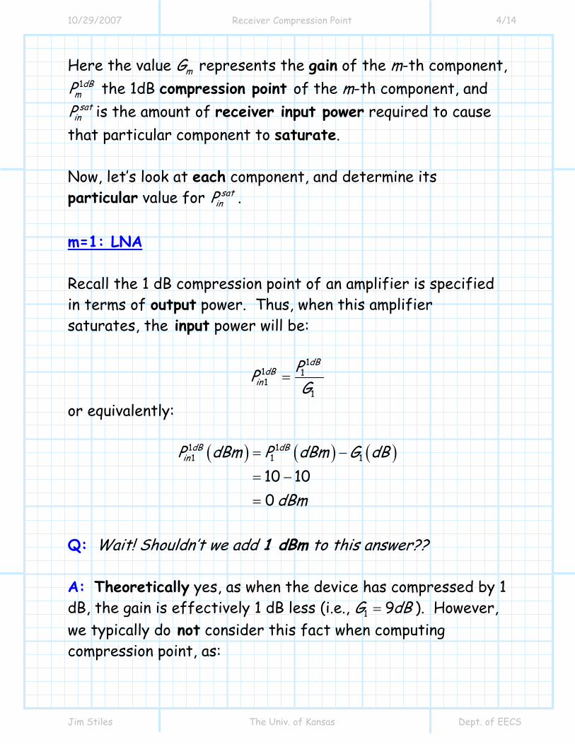
Here the value mG represents the gain of the m-th component, 1dB

mP the 1dB compression point of the m-th component, and sat

inP is the amount of receiver input power required to cause that particular component to saturate. Now, let’s look at each component, and determine its particular value for sat

inP . m=1: LNA Recall the 1 dB compression point of an amplifier is specified in terms of output power. Thus, when this amplifier saturates, the input power will be:

11 11

1

dBdB

inPPG

=

or equivalently:

( ) ( ) ( )1 11 1 1

10 100

dB dBinP dBm P dBm G dB

dBm

= −

= −

=

Q: Wait! Shouldn’t we add 1 dBm to this answer?? A: Theoretically yes, as when the device has compressed by 1 dB, the gain is effectively 1 dB less (i.e., 1 9G dB= ). However, we typically do not consider this fact when computing compression point, as:



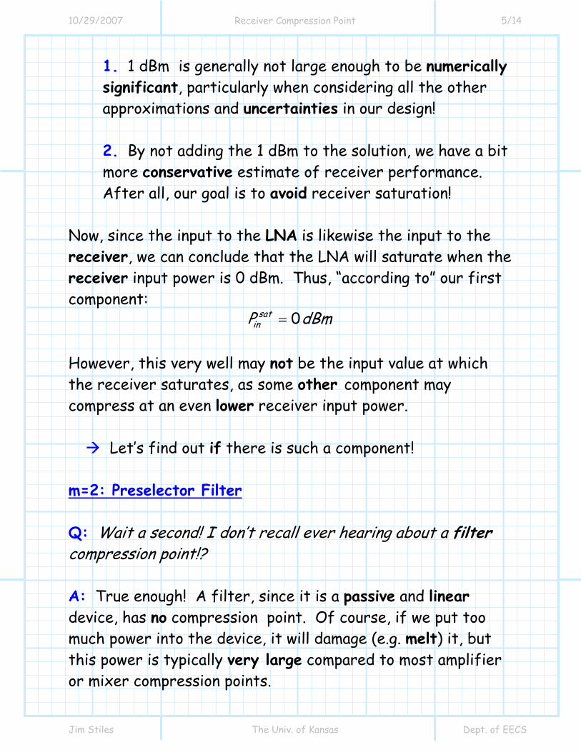
1. 1 dBm is generally not large enough to be numerically significant, particularly when considering all the other approximations and uncertainties in our design! 2. By not adding the 1 dBm to the solution, we have a bit more conservative estimate of receiver performance. After all, our goal is to avoid receiver saturation!

Now, since the input to the LNA is likewise the input to the receiver, we can conclude that the LNA will saturate when the receiver input power is 0 dBm. Thus, “according to” our first component:

0satinP dBm=

However, this very well may not be the input value at which the receiver saturates, as some other component may compress at an even lower receiver input power.

Let’s find out if there is such a component! m=2: Preselector Filter Q: Wait a second! I don’t recall ever hearing about a filter compression point!? A: True enough! A filter, since it is a passive and linear device, has no compression point. Of course, if we put too much power into the device, it will damage (e.g. melt) it, but this power is typically very large compared to most amplifier or mixer compression points.



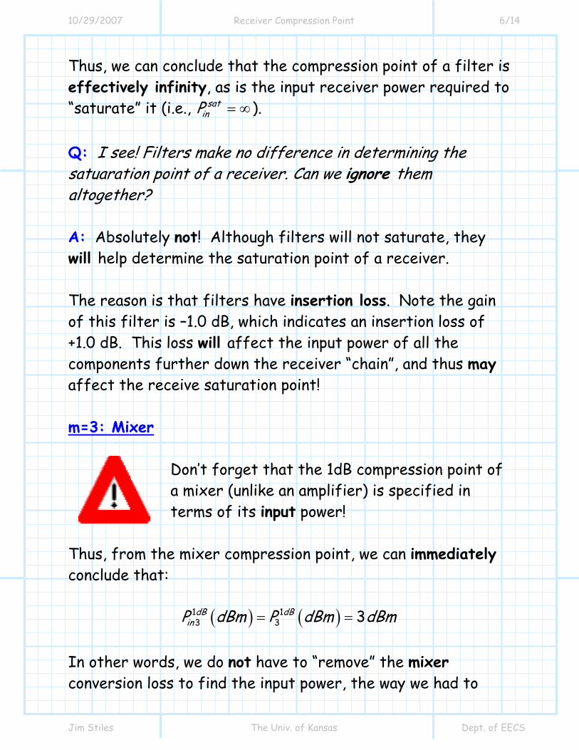
Thus, we can conclude that the compression point of a filter is effectively infinity, as is the input receiver power required to “saturate” it (i.e., sat

inP = ∞ ). Q: I see! Filters make no difference in determining the satuaration point of a receiver. Can we ignore them altogether? A: Absolutely not! Although filters will not saturate, they will help determine the saturation point of a receiver. The reason is that filters have insertion loss. Note the gain of this filter is –1.0 dB, which indicates an insertion loss of +1.0 dB. This loss will affect the input power of all the components further down the receiver “chain”, and thus may affect the receive saturation point! m=3: Mixer

Don’t forget that the 1dB compression point of a mixer (unlike an amplifier) is specified in terms of its input power!

Thus, from the mixer compression point, we can immediately conclude that:

( ) ( )1 13 3 3dB dB

inP dBm P dBm dBm= =

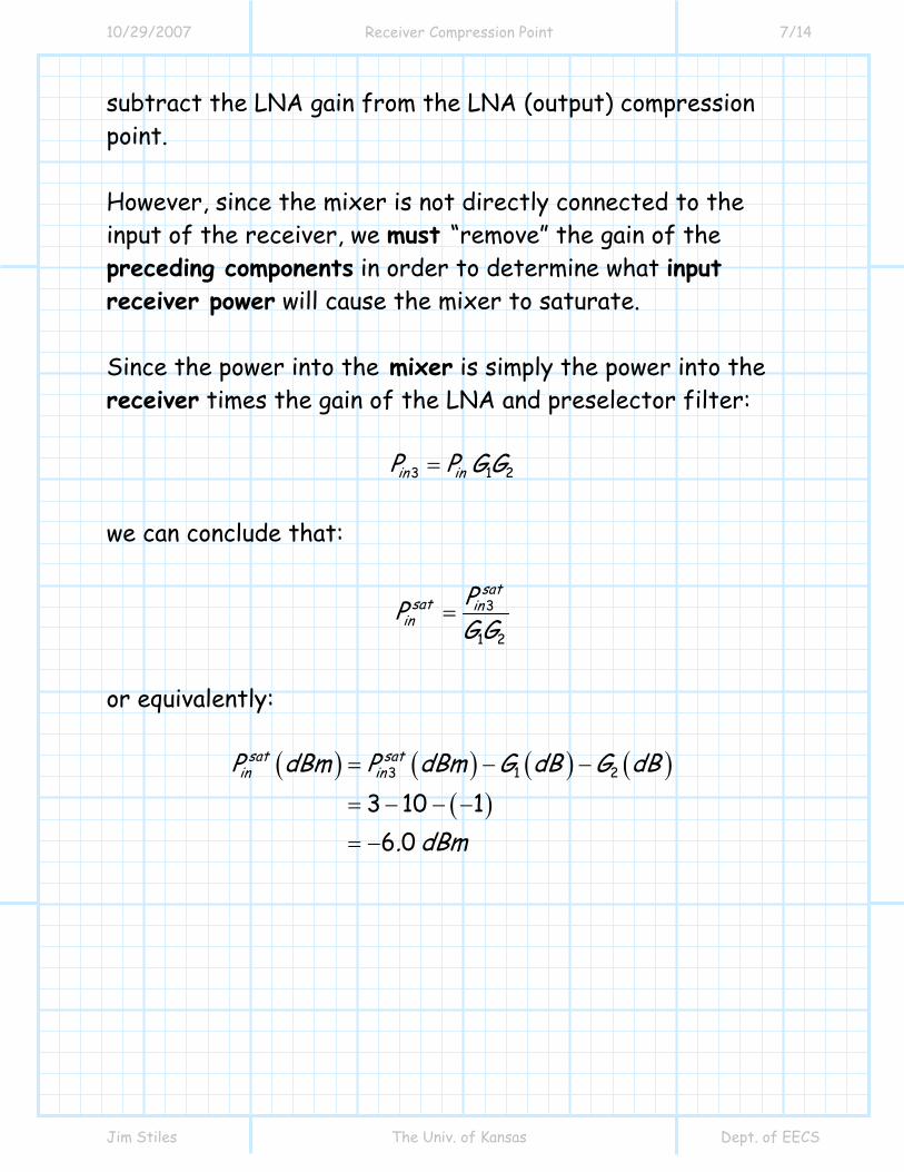
In other words, we do not have to “remove” the mixer conversion loss to find the input power, the way we had to



subtract the LNA gain from the LNA (output) compression point. However, since the mixer is not directly connected to the input of the receiver, we must “remove” the gain of the preceding components in order to determine what input receiver power will cause the mixer to saturate. Since the power into the mixer is simply the power into the receiver times the gain of the LNA and preselector filter:

3 1 2in inP P G G= we can conclude that:

3

1 2

satsat in

inPPG G

=

or equivalently:

( ) ( ) ( ) ( )( )

3 1 2

3 10 16 0

sat satin inP dBm P dBm G dB G dB

. dBm

= − −

= − − −

= −



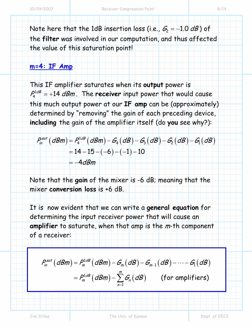
Note here that the 1dB insertion loss (i.e., 2 1 0G . dB= − ) of the filter was involved in our computation, and thus affected the value of this saturation point! m=4: IF Amp This IF amplifier saturates when its output power is

14 14dBP dBm= + . The receiver input power that would cause

this much output power at our IF amp can be (approximately) determined by “removing” the gain of each preceding device, including the gain of the amplifier itself (do you see why?):

( ) ( ) ( ) ( ) ( ) ( )( ) ( )

13 2 14 4

14 15 6 1 104

sat dBinP dBm P dBm G dB G dB G dB G dB

dBm

= − − − −

= − − − − − −

= −

Note that the gain of the mixer is -6 dB; meaning that the mixer conversion loss is +6 dB. It is now evident that we can write a general equation for determining the input receiver power that will cause an amplifier to saturate, when that amp is the m-th component of a receiver:

( ) ( ) ( ) ( ) ( )

( ) ( )

11 1

1

1(for amplifiers)

sat dBin m m m

mdB

m nn

P dBm P dBm G dB G dB G dB

P dBm G dB

−

=

= − − − −

= −∑



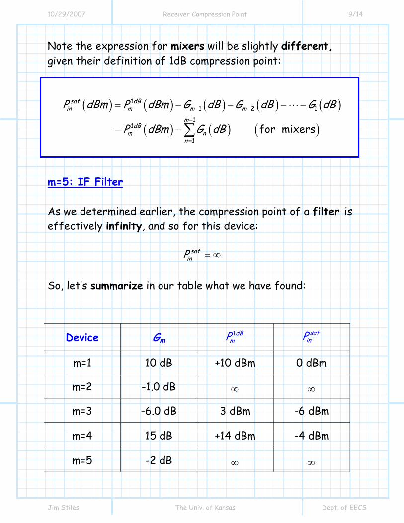
Note the expression for mixers will be slightly different, given their definition of 1dB compression point:

( ) ( ) ( ) ( ) ( )

( ) ( ) ( )

11 2 1

11

1for mixers

sat dBin m m m

mdB

m nn

P dBm P dBm G dB G dB G dB

P dBm G dB

− −

−

=

= − − − −

= −∑

m=5: IF Filter As we determined earlier, the compression point of a filter is effectively infinity, and so for this device:

satinP = ∞

So, let’s summarize in our table what we have found:

Device Gm 1dBmP sat

inP

m=1 10 dB +10 dBm 0 dBm

m=2 -1.0 dB ∞ ∞

m=3 -6.0 dB 3 dBm -6 dBm

m=4 15 dB +14 dBm -4 dBm

m=5 -2 dB ∞ ∞



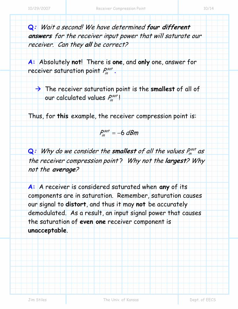
Q: Wait a second! We have determined four different answers for the receiver input power that will saturate our receiver. Can they all be correct? A: Absolutely not! There is one, and only one, answer for receiver saturation point sat

inP .

The receiver saturation point is the smallest of all of our calculated values sat

inP ! Thus, for this example, the receiver compression point is:

6satinP dBm= −

Q: Why do we consider the smallest of all the values sat

inP as the receiver compression point ? Why not the largest? Why not the average? A: A receiver is considered saturated when any of its components are in saturation. Remember, saturation causes our signal to distort, and thus it may not be accurately demodulated. As a result, an input signal power that causes the saturation of even one receiver component is unacceptable.



Thus, by choosing the smallest of the input saturation powers, we have selected a value that will unambiguously define the point where even one component is saturated—if the receiver input power is less than even the smallest of our calculated

satinP , then none of the receiver components will be saturated.

Q: In this example, it is the mixer that saturates first. Is this always the case? A: It is indeed often the case that the mixer is the device that determines the receiver saturation point. However, the LNA can likewise be the component that saturates first. Q: What can we do to improve (i.e., increase) the saturation point of a receiver? A: Considering the discussion of this handout, it should be quite evident how to accomplish this. We can do two different things: 1. Find a different component part with a higher saturation point 1dB

mP This strategy at first seems very simple. However, a component designer of mixers or amplifiers is faced with the same design conflicts and trade-offs that typically face all other design engineers. If he or she improves the 1dB compression point, it will undoubtedly mess-up some other



important parameter like gain, or bandwidth, or noise figure, or conversion loss. Thus, a receiver designer that attempts to replace a mixer or amplifier with another exhibiting a higher 1dB compression point will almost certainly cause some degradation in some other receiver performance parameter, like gain, or noise figure, or bandwidth.

The selection of receiver component parts is typically a compromise between competing and conflicting component parameters. You will never find a “perfect” microwave component, only a component which best suits the receiver specifications and design goals.

2. Decrease the gain (increase the attenuation) of the component parts preceding the component that saturates. Decreasing the gain and or increasing the loss of components in a receiver will generally improve (i.e, increase) the receiver saturation point. However, it will also mess-up the receiver noise figure and MDS!

Again, we are faced with a design trade-off! Note however, that we only need to decrease the total gain of the components preceding the device that is saturating. Another way to accomplish this is simply to rearrange the order of the devices in the receiver chain.



For example, we might move an amplifier from a location preceding the saturating component, to a location after the saturating component—this of course reduces the gain of the components preceding the device, but does not alter the overall receiver gain! Likewise, we might move a lossy component from a location after a saturating component, to a location preceding the saturating component—this again reduces the gain of the components preceding the device, but again does not alter the overall receiver gain! Thus, we can conclude that the compression point of a receiver will typically improve if we move lossy components to the front and amplifiers to the back! However, we must keep in mind two things: * The order of some devices cannot be changed. For example, we cannot put the mixer before the preselector filter! * Although rearranging the order of the components in a receiver will not change the receiver gain, it can play havoc with receiver noise figure and MDS! In fact, it should be evident to you that the receiver noise figure typically improves if we move lossy components to the back and amplifiers to the front—exactly the opposite strategy for improving receiver saturation!



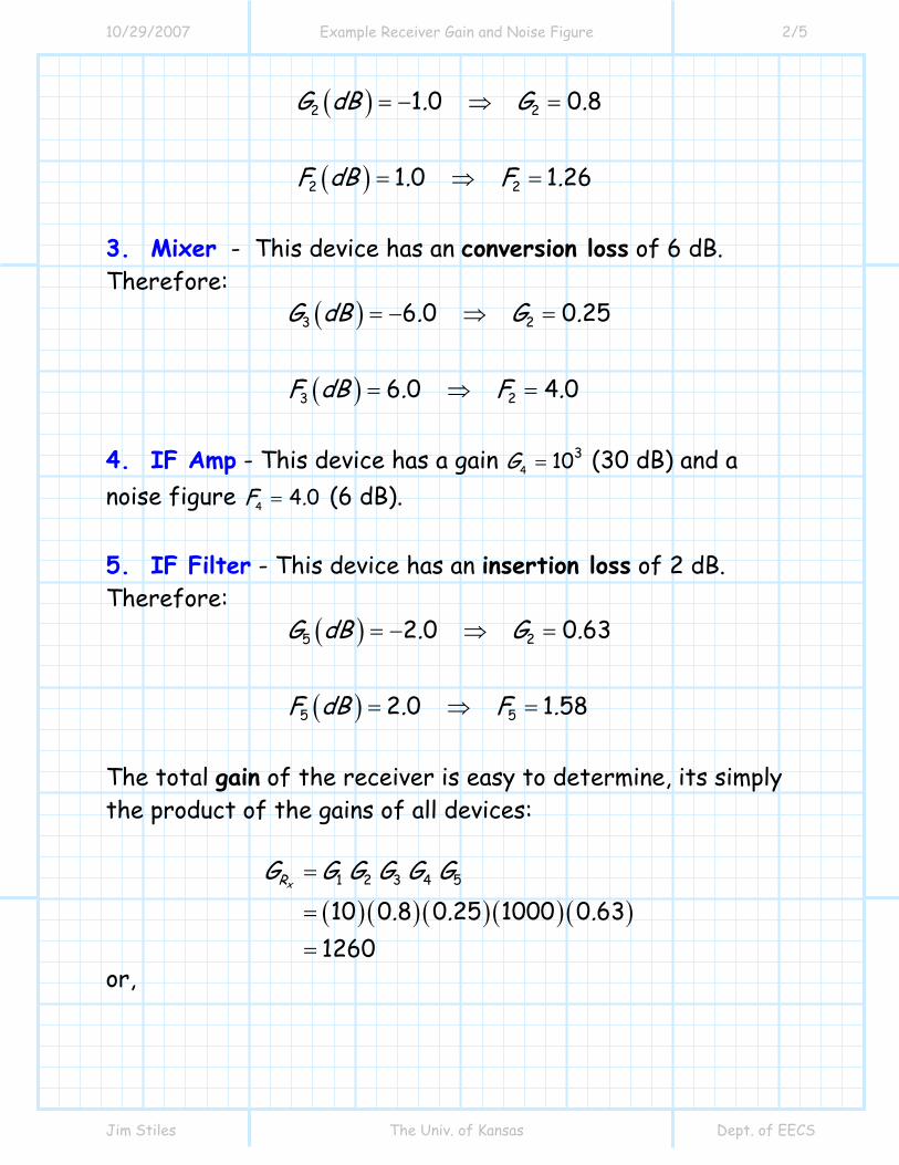
We find that very often, receiver saturation point and receiver sensitivity are in direct conflict—improve one and you degrade the other!

Saturation Point

Sensitivity

10/29/2007 Receiver Dynamic Range 1/1


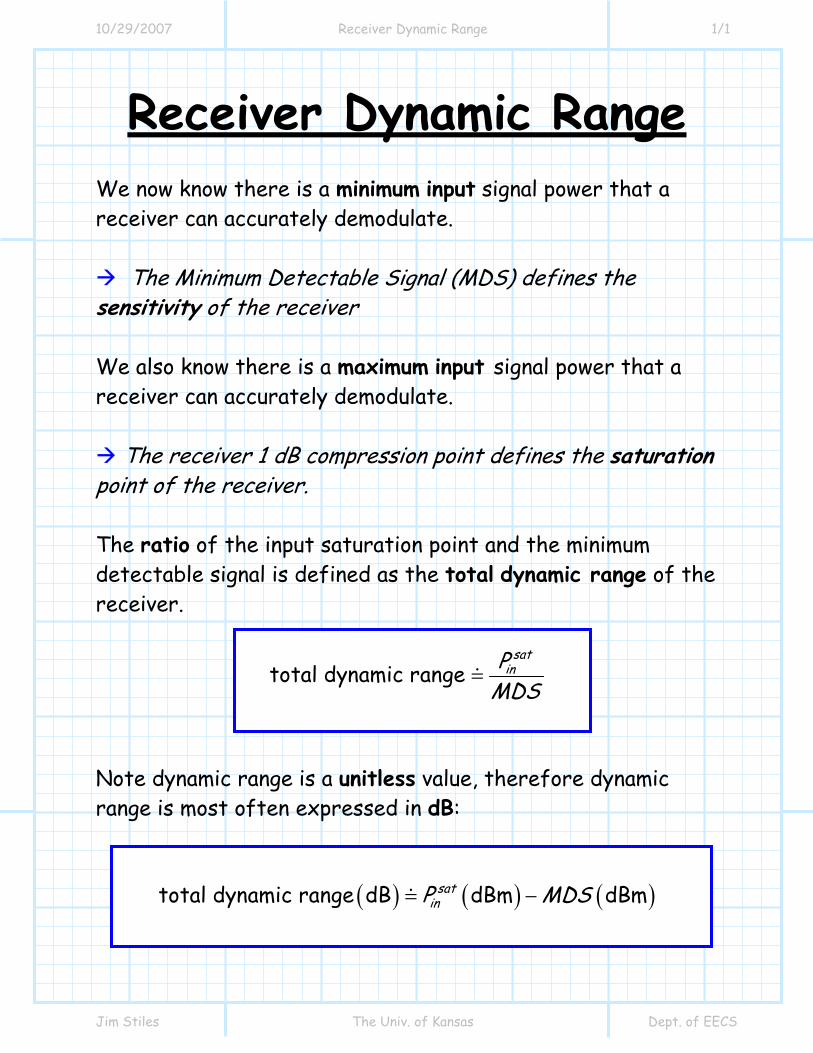
Receiver Dynamic Range We now know there is a minimum input signal power that a receiver can accurately demodulate.

The Minimum Detectable Signal (MDS) defines the sensitivity of the receiver We also know there is a maximum input signal power that a receiver can accurately demodulate.

The receiver 1 dB compression point defines the saturation point of the receiver. The ratio of the input saturation point and the minimum detectable signal is defined as the total dynamic range of the receiver.

total dynamic rangesat

inPMDS

Note dynamic range is a unitless value, therefore dynamic range is most often expressed in dB:

( ) ( ) ( )total dynamic range dB dBm dBmsatinP MDS−

Documents

D. Receiver Dynamic Range