Embed Size (px)
Citation preview
D-Lab & D-Lab Control Plan. Measure. Analyse
User Manual
Valid for
D-Lab Versions 2.0 and 2.1
September 2011
Contents
1
Contents 1 Initial Steps ...................................................................................................................................... 6
1.1 Scope of Supply ....................................................................................................................... 6
1.1.1 Optional Upgrades ........................................................................................................... 6
1.1.2 Accessories ...................................................................................................................... 6
1.2 System Requirements.............................................................................................................. 7
1.3 Installation ............................................................................................................................... 7
2 Incorporation of D-LAB and D-Lab Control in the Study ................................................................. 9
2.1 D-Lab Modules and Structure ............................................................................................... 11
2.1.1 Eye Tracking Module ..................................................................................................... 12
2.1.2 Video Module ................................................................................................................ 13
2.1.3 Data Stream Module ..................................................................................................... 14
3 PLAN - Preparing a Study ............................................................................................................... 15
3.1 Preparing the Test Environment ........................................................................................... 15
3.1.1 Starting Up the Eye Tracking Module ............................................................................ 15
3.1.1.1 Positioning the Markers ............................................................................................ 15
3.1.2 Preparing the Video Module ......................................................................................... 18
3.1.3 Preparing for Data Stream Recording ........................................................................... 18
3.2 Creating a Test Procedure ..................................................................................................... 20
3.2.1 Organizing the Test Procedure ...................................................................................... 20
3.2.2 Creating a New Test Procedure ..................................................................................... 21
3.2.3 Organizing a Test Procedure ......................................................................................... 22
3.2.4 Saving a Test Procedure ................................................................................................ 23
3.2.5 Opening an Existing Test Procedure .............................................................................. 23
4 MEASURE – Recording Data with D-Lab Control ........................................................................... 25
4.1 D-Lab Control - Modules and Structure ................................................................................ 26
4.2 Setting Up a Connection with the Video Module .................................................................. 27
4.3 Setting Up a Connection with the Dikablis Recorder ............................................................ 28
4.4 Setting Up a Connection with the Video Stream Module ..................................................... 29
4.5 Setting Up the Dikablis Remote Connection ......................................................................... 29
4.6 Study Management ............................................................................................................... 29
4.7 Structure of the Data in D-Lab Control .................................................................................. 30
4.8 Creating a New Project (Study) ............................................................................................. 30
4.9 Creating a New Experiment (Subject) ................................................................................... 31
Contents
2
4.10 Opening a Project .................................................................................................................. 32
4.11 Recording Data ...................................................................................................................... 32
4.12 Opening a Test Procedure ..................................................................................................... 33
4.13 Marking Use Case Intervals ................................................................................................... 34
5 ANALYSE –Data Analysis ................................................................................................................ 36
5.1 Eye Tracking Module ............................................................................................................. 36
5.1.1 Validating the Eye Tracking Data ................................................................................... 37
5.1.2 Marker Detection .......................................................................................................... 37
5.1.3 Importing the Eye Tracking Data ................................................................................... 39
5.1.4 Saving a Project ............................................................................................................. 41
5.1.5 Opening a Project .......................................................................................................... 41
5.1.6 Playing Back Eye Tracking Data ..................................................................................... 41
5.1.6.1 Player Functions ........................................................................................................ 42
5.1.7 Audio Playback .............................................................................................................. 43
5.1.8 Managing Use Case Intervals......................................................................................... 43
5.1.8.1 Importing a Test Procedure ....................................................................................... 44
5.1.8.2 Visualizing the Use Cases ........................................................................................... 45
5.1.8.3 Adjusting the Use Cases ............................................................................................ 46
5.1.8.4 Creating New Use Cases ............................................................................................ 47
5.1.8.5 Deleting Tasks ............................................................................................................ 48
5.1.9 Defining Combined Markers .......................................................................................... 48
5.1.10 Organizing Areas of Interest .......................................................................................... 49
5.1.10.1 Area of Validity ...................................................................................................... 50
5.1.10.2 Defining AOIs ......................................................................................................... 51
5.1.10.3 Changing AOIs ........................................................................................................ 53
5.1.10.4 Deleting AOIs ......................................................................................................... 54
5.1.11 Computing the Glances toward the AOIs ...................................................................... 54
5.1.11.1 Deleting Blinks ....................................................................................................... 54
5.1.11.2 Deleting "Cross Throughs" ..................................................................................... 55
5.1.12 Visualizing the Glance Behavior .................................................................................... 56
5.1.12.1 Validity Index for Markers and Pupil Detection .................................................... 56
5.1.13 Manual Glance Setting .................................................................................................. 57
5.1.13.1 Creating New Glances............................................................................................ 57
5.1.13.2 Adjusting Existing Glances ..................................................................................... 58
5.1.13.3 Deleting the Glance ............................................................................................... 58
Contents
3
5.1.14 Computing Eye-Tracking Statistics ................................................................................ 58
5.1.14.1 Use Case Selection ................................................................................................. 59
5.1.14.2 AOI Selection ......................................................................................................... 59
5.1.14.3 Statistics Selection ................................................................................................. 60
5.1.14.4 Visualizing Eye-Tracking Statistics ......................................................................... 61
5.1.14.5 Exporting the Eye-Tracking Statistics .................................................................... 61
5.1.15 Creating a Gaze Motion Trend ...................................................................................... 63
5.1.16 Heat Map Visualization.................................................................................................. 63
5.2 D-Lab Video Module .............................................................................................................. 69
5.2.1 Importing the Video Data .............................................................................................. 69
5.2.2 Video Playback............................................................................................................... 73
5.2.3 Activity Analysis ............................................................................................................. 73
5.2.3.1 Defining an Activity Group ........................................................................................ 74
5.2.3.2 Defining an Activity.................................................................................................... 75
5.2.3.3 MarkingAactivities ..................................................................................................... 77
5.2.3.4 Computing and Exporting Statistics .......................................................................... 80
5.3 D-Lab Data Stream Module ................................................................................................... 82
5.3.1 Importing Data Streams ................................................................................................ 82
5.3.1.1 Defining a Configuration............................................................................................ 82
5.3.1.2 Importing Data .......................................................................................................... 84
5.3.2 Visualizing Data ............................................................................................................. 87
5.3.3 Computing the Statistics ................................................................................................ 88
5.3.3.1 Data Stream Statistical Values ................................................................................... 90
6 Extended Functions ....................................................................................................................... 91
6.1 Export Raw ............................................................................................................................ 91
6.2 Marker Co-Ordinate System .................................................................................................. 91
6.2.1 Export Gaze Data ........................................................................................................... 93
6.3 Export Validity Index ............................................................................................................. 94
Glossary ................................................................................................................................................. 95
Appendix A - D-Lab Control Network Interface ..................................................................................... 96
Marking Use Case Intervals ............................................................................................................... 96
Remotely Marking Use Cases ............................................................................................................ 97
Remote Control of Dikablis Recording Software ............................................................................... 98
Appendix B - Data Stream Interface .................................................................................................... 100
Appendix C - D-Lab Markers ................................................................................................................ 103
Contents
4
5
Dear customer,
Thank you for choosing to purchase our product. The "D-Lab" analysis software and "D-Lab Control"
control software will provide you with optimum support for your behavioral research experiments
from the planning stage and the carrying out of the experiments themselves, right through to the
optimum automatic evaluation of the gathered data. Our products guarantee maximum performance
and convenience.
With our D-Lab and D-Lab Control, we at Ergoneers are providing you with a complete and consistent
software system for the scientific analysis of behavioral data such as eye tracking data, video data
and information on the surroundings (e.g. data taken from a driving or flying simulation). D-Lab
Module Eye Tracking, Video and Data Stream can be used to record, visualize and analyze the data
from the corresponding sensors synchronously.
Thank you for putting your trust in our product. We hope you enjoy using your new D-Lab und D-Lab
Control Software Suite.
Your team from Ergoneers
Scope of Supply
6
1 Initial Steps
1.1 Scope of Supply
Your order comes with the following components:
- D-Lab, marker detector and D-Lab Control installation CD
- D-Lab license stick
- Four D-Lab markers (only in combination with the D-Lab eye tracking module)
If you ordered additional hardware in combination with a D-Lab module, please refer to section 1.1.2
Accessories.
1.1.1 Optional Upgrades
D-Lab functions can be expanded at any time by purchasing additional modules. Should you choose
to do so, you will receive a software update and a new license stick. It goes without saying that you
will also be able to continue processing all existing D-Lab projects with the expanded version.
1.1.2 Accessories
Depending on the D-Lab module purchased (see section 2.1), we can offer you the following optional
accessories:
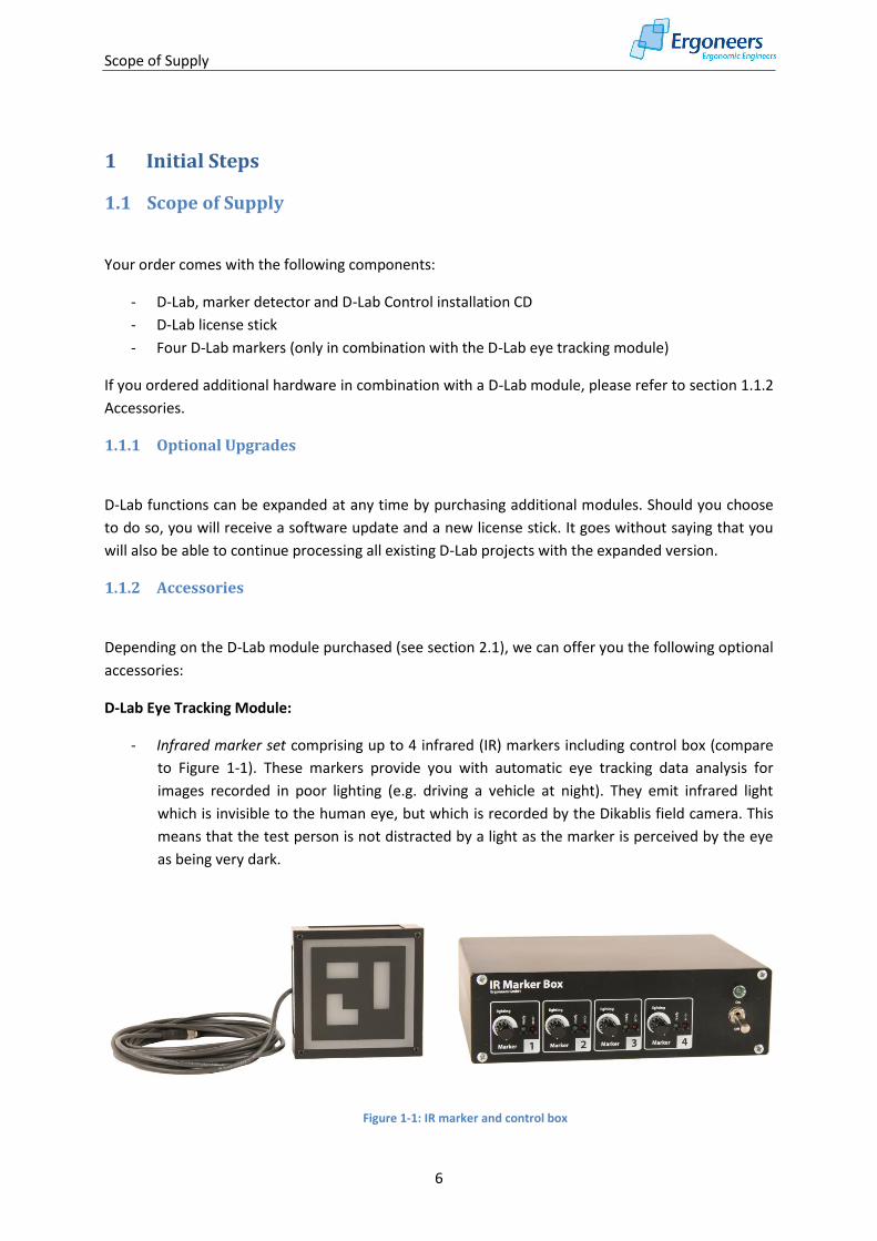
D-Lab Eye Tracking Module:
- Infrared marker set comprising up to 4 infrared (IR) markers including control box (compare
to Figure 1-1). These markers provide you with automatic eye tracking data analysis for
images recorded in poor lighting (e.g. driving a vehicle at night). They emit infrared light
which is invisible to the human eye, but which is recorded by the Dikablis field camera. This
means that the test person is not distracted by a light as the marker is perceived by the eye
as being very dark.
Figure 1-1: IR marker and control box
System Requirements
7
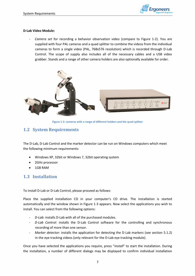
D-Lab Video Module:
- Camera set for recording a behavior observation video (compare to Figure 1-2). You are
supplied with four PAL cameras and a quad splitter to combine the videos from the individual
cameras to form a single video (PAL, 768x576 resolution) which is recorded through D-Lab
Control. The scope of supply also includes all of the necessary cables and a USB video
grabber. Stands and a range of other camera holders are also optionally available for order.
Figure 1-2: cameras with a range of different holders and the quad splitter
1.2 System Requirements
The D-Lab, D-Lab Control and the marker detector can be run on Windows computers which meet
the following minimum requirements:
Windows XP, 32bit or Windows 7, 32bit operating system
2GHz processor
1GB RAM
1.3 Installation
To install D-Lab or D-Lab Control, please proceed as follows:
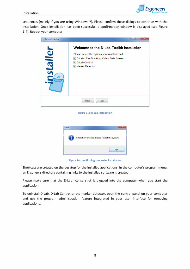
Place the supplied installation CD in your computer's CD drive. The installation is started
automatically and the window shown in Figure 1-3 appears. Now select the applications you wish to
install. You can select from the following options:
- D-Lab: installs D-Lab with all of the purchased modules.
- D-Lab Control: installs the D-Lab Control software for the controlling and synchronous
recording of more than one sensor.
- Marker detector: installs the application for detecting the D-Lab markers (see section 5.1.2)
in the eye tracking videos (only relevant for the D-Lab eye tracking module).
Once you have selected the applications you require, press "Install" to start the installation. During
the installation, a number of different dialogs may be displayed to confirm individual installation
Installation
8
sequences (mainly if you are using Windows 7). Please confirm these dialogs to continue with the
installation. Once installation has been successful, a confirmation window is displayed (see Figure
1-4). Reboot your computer.
Figure 1-3: D-Lab installation
Figure 1-4: confirming successful installation
Shortcuts are created on the desktop for the installed applications. In the computer's program menu,
an Ergoneers directory containing links to the installed software is created.
Please make sure that the D-Lab license stick is plugged into the computer when you start the
application.
To uninstall D-Lab, D-Lab Control or the marker detector, open the control panel on your computer
and use the program administration feature integrated in your user interface for removing
applications.
Installation
9
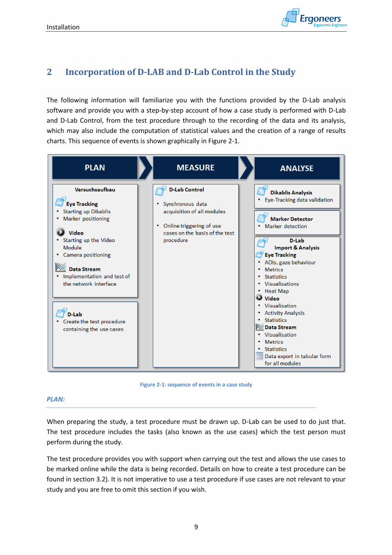
2 Incorporation of D-LAB and D-Lab Control in the Study
The following information will familiarize you with the functions provided by the D-Lab analysis
software and provide you with a step-by-step account of how a case study is performed with D-Lab
and D-Lab Control, from the test procedure through to the recording of the data and its analysis,
which may also include the computation of statistical values and the creation of a range of results
charts. This sequence of events is shown graphically in Figure 2-1.
Figure 2-1: sequence of events in a case study
PLAN:
When preparing the study, a test procedure must be drawn up. D-Lab can be used to do just that.
The test procedure includes the tasks (also known as the use cases) which the test person must
perform during the study.
The test procedure provides you with support when carrying out the test and allows the use cases to
be marked online while the data is being recorded. Details on how to create a test procedure can be
found in section 3.2). It is not imperative to use a test procedure if use cases are not relevant to your
study and you are free to omit this section if you wish.
Installation
10
The preparation and testing of the test set-up are vital for ensuring the success of a case study. To
record the eye tracking data, Dikablis must firstly be started up (see the Dikablis User Manual) and
the markers must be positioned correctly (details can be found in section 3.1.1.1). If the video
module is used, the cameras must firstly be set up and positioned (see section 3.1.2). Should you
wish to record an additional data stream (e.g. driving dynamics data) in synchronization with the eye
tracking data, we recommend a test with the Data Stream interface (see section 3.1.3).
MEASURE:
Once all of the precautionary measures have been taken, the study can be started. The data is
recorded with D-Lab Control and thus ensures that all of the modules are in synchronization with one
another. The use case intervals can be marked during recording. These marks can be retained in the
recorded data and then used at a later stage for analysis purposes.
ANALYSIS:
Before the actual data analysis is performed, we recommend validating the eye tracking data. With
the Dikablis analysis software, the eye tracking data can be checked and, if necessary, the calibration
or the pupil detection can be improved (for details, see the Dikablis manual).
The detection of the markers in the recorded eye tracking videos must also be included in the
preparation of the analysis. To do so, use the marker detector (see section 5.1.2).
The data from all of the modules can then be imported into D-Lab (see 5.1.3 for the eye tracking
data, section 5.2.1 for the video module and section 5.3.1 for data stream importing) and analyzed.
First of all, the use case intervals (if supplied) should be validated (see section 5.1.1).
Areas of interest can now be defined for the eye tracking data. Glances in the direction of these areas
of interest are automatically counted. The glance characteristics and statistics can then be computed
for the defined use cases and exported in table form. There are a number of different graphs and
heat maps available for visualizing the results. Details on how to analyze the eye tracking data can be
found in section 5.1).
The recorded video data can be visualized in synchronization with the eye tracking data. To examine
behavior using this video, you will need the behavior analysis module (see section 5.2).
There are several different characteristics available for the data recorded with the Data Stream
module. In a similar way as for the eye tracking data, they can be computed for selected use cases
and then exported in table form. The development of the data can also be displayed in graph form
over the time sequence. Details on the Data Stream module can be found in section 5.3).
The modules making up a behavioral study (PLAN, MEASURE and ANALYSE) are explained in detail in
the subsequent sections of this manual.
D-Lab Modules and Structure
11
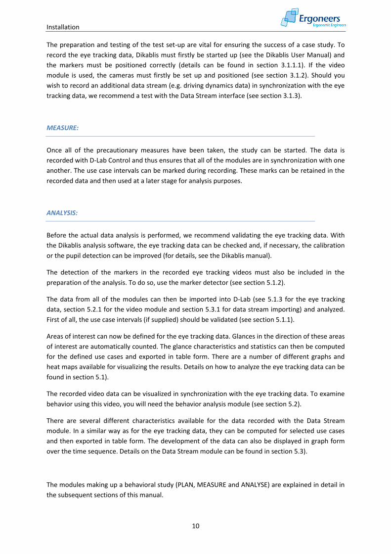
2.1 D-Lab Modules and Structure
D-Lab comprises a basic package, D-Lab Eye Tracking, and can be optionally expanded to include the
Video and Data Stream modules. The following areas and functions from the D-Lab user interface
(see Figure 2-2) are available for all modules:
- Menu bar with entries for project management and access to a number of different module
functions
- Toolbar for quick access to a range of functions
- The "Project overview" and "Test procedure" tabs, which are positioned in the left section of
the window. The former displays the structure of the current project and offers navigation
options. The latter is used for planning purposes and allows a test procedure to be drawn up.
- The use case functions which can be found in the tabs "Use cases" (in the right window
section)" and “Use Case visualisation" (in the middle of the bottom window section). In the
"Use cases" section, all of the defined use case intervals and results are listed together with
an option to either change or redefine them. The "Use case visualisation" tab is used for
displaying the use case intervals.
Figure 2-2: D-Lab, intermodular areas
D-Lab Modules and Structure
12
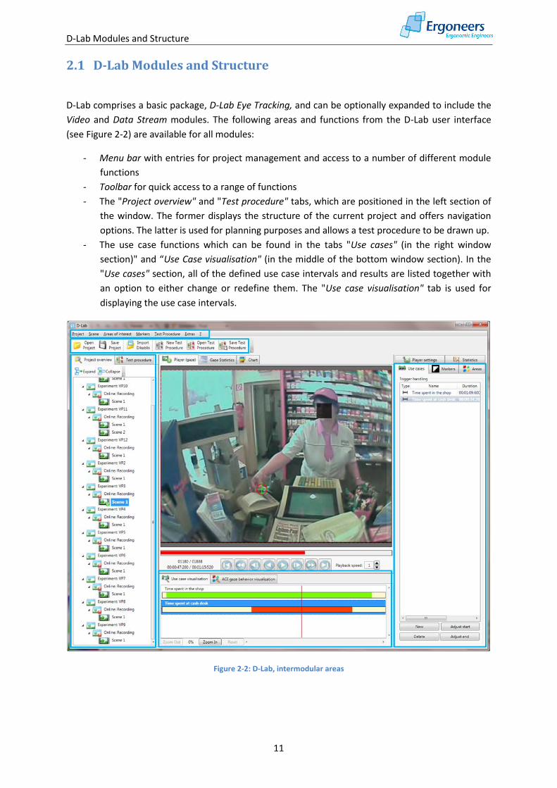
2.1.1 Eye Tracking Module
The eye tracking module supports the analysis of the eye tracking data recorded with Dikablis. The
D-Lab user interface for the eye-tracking basic package is shown in Figure 2-3 and has the following
structure and functions:
- The "Player", "Gaze statistics" and "Chart" tabs are positioned in the top center area of the
screen. In the "Player", the eye tracking video selected in the "Project overview" is shown
and the detected markers, the defined areas of interest (AOIs) and the heat map are
displayed. The "Gaze statistics" tab is used for displaying the automatically computed
inference and descriptive statistics for a selectable number of eye tracking characteristics.
The "Chart" tab displays the eye tracking development diagrams.
Figure 2-3: overview of the D-Lab eye tracking module
- The "AOI gaze behavior visualisation" tab in the bottom center window section displays the
glances towards the defined AOIs.
- The right section of the window includes several tabs and contains the most D-Lab functions.
In the "Markers" section, all of the detected markers are displayed and combined markers
can be defined.
Areas of interest are defined and edited in the "Areas" tab. In the same tab, the
automatically computed durations of the glances towards the AOIs are displayed in list form
and a manual adjustment of these values is possible.
The settings for the heat map are made in the "Player settings" tab. Using the heat map, the
test person's gaze can be observed over a pre-settable time interval while the video is
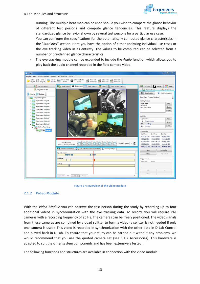
D-Lab Modules and Structure
13
running. The multiple heat map can be used should you wish to compare the glance behavior
of different test persons and compute glance tendencies. This feature displays the
standardized glance behavior shown by several test persons for a particular use case.
You can configure the specifications for the automatically computed glance characteristics in
the "Statistics" section. Here you have the option of either analyzing individual use cases or
the eye tracking video in its entirety. The values to be computed can be selected from a
number of pre-defined glance characteristics.
- The eye tracking module can be expanded to include the Audio function which allows you to
play back the audio channel recorded in the field camera video.
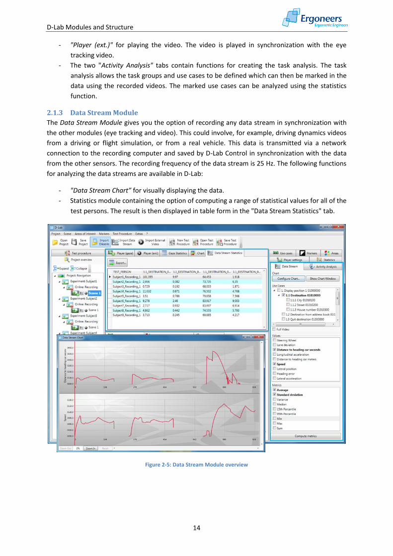
Figure 2-4: overview of the video module
2.1.2 Video Module
With the Video Module you can observe the test person during the study by recording up to four
additional videos in synchronization with the eye tracking data. To record, you will require PAL
cameras with a recording frequency of 25 Hz. The cameras can be freely positioned. The video signals
from these cameras are combined by a quad splitter to form a video (a splitter is not needed if only
one camera is used). This video is recorded in synchronization with the other data in D-Lab Control
and played back in D-Lab. To ensure that your study can be carried out without any problems, we
would recommend that you use the quoted camera set (see 1.1.2 Accessories). This hardware is
adapted to suit the other system components and has been extensively tested.
The following functions and structures are available in connection with the video module:
D-Lab Modules and Structure
14
- "Player (ext.)" for playing the video. The video is played in synchronization with the eye
tracking video.
- The two "Activity Analysis" tabs contain functions for creating the task analysis. The task
analysis allows the task groups and use cases to be defined which can then be marked in the
data using the recorded videos. The marked use cases can be analyzed using the statistics
function.
2.1.3 Data Stream Module
The Data Stream Module gives you the option of recording any data stream in synchronization with
the other modules (eye tracking and video). This could involve, for example, driving dynamics videos
from a driving or flight simulation, or from a real vehicle. This data is transmitted via a network
connection to the recording computer and saved by D-Lab Control in synchronization with the data
from the other sensors. The recording frequency of the data stream is 25 Hz. The following functions
for analyzing the data streams are available in D-Lab:
- "Data Stream Chart” for visually displaying the data.
- Statistics module containing the option of computing a range of statistical values for all of the
test persons. The result is then displayed in table form in the "Data Stream Statistics" tab.
Figure 2-5: Data Stream Module overview
Preparing the Test Environment
15
3 PLAN - Preparing a Study
When preparing a case study, the test scenario must be set up and test procedure must be planned.
If the use of a planned test procedure is optional, the test environment must be well prepared for
the study to be a success.
3.1 Preparing the Test Environment
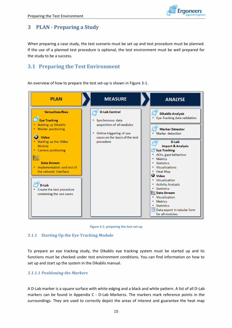
An overview of how to prepare the test set-up is shown in Figure 3-1.
Figure 3-1: preparing the test set-up
3.1.1 Starting Up the Eye Tracking Module
To prepare an eye tracking study, the Dikablis eye tracking system must be started up and its
functions must be checked under test environment conditions. You can find information on how to
set up and start up the system in the Dikablis manual.
3.1.1.1 Positioning the Markers
A D-Lab marker is a square surface with white edging and a black and white pattern. A list of all D-Lab
markers can be found in Appendix C - D-Lab Markerss. The markers mark reference points in the
surroundings. They are used to correctly depict the areas of interest and guarantee the heat map
Preparing the Test Environment
16
even though the test persons may be moving their heads. Markers are detected in the eye tracking
videos using image processing technology (see section 5.1.2). Both the AOIs and the heat map are
connected to the detected markers. This is why it is extremely important to position the markers in
the test environment if the eye tracking data is to be evaluated correctly. To ensure that the markers
are successfully detected, please observe the following guidelines on marker positioning:
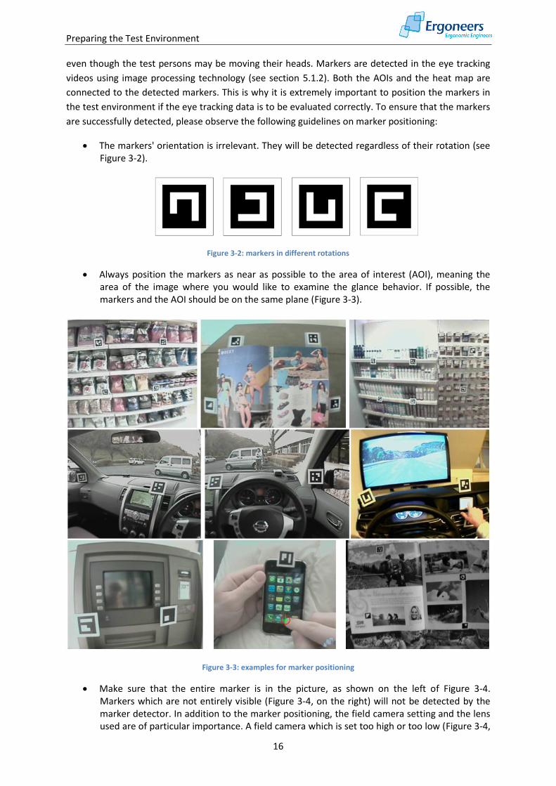
The markers' orientation is irrelevant. They will be detected regardless of their rotation (see Figure 3-2).
Figure 3-2: markers in different rotations
Always position the markers as near as possible to the area of interest (AOI), meaning the area of the image where you would like to examine the glance behavior. If possible, the markers and the AOI should be on the same plane (Figure 3-3).
Figure 3-3: examples for marker positioning
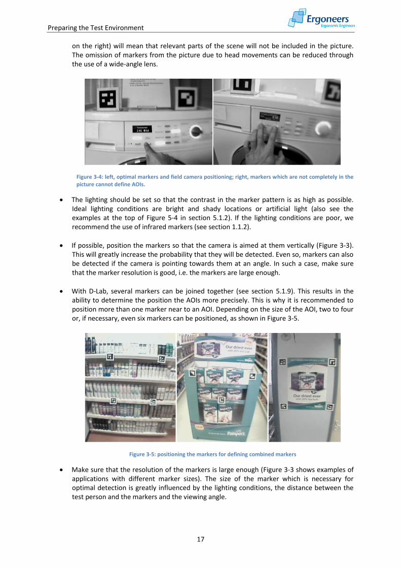
Make sure that the entire marker is in the picture, as shown on the left of Figure 3-4. Markers which are not entirely visible (Figure 3-4, on the right) will not be detected by the marker detector. In addition to the marker positioning, the field camera setting and the lens used are of particular importance. A field camera which is set too high or too low (Figure 3-4,
Preparing the Test Environment
17
on the right) will mean that relevant parts of the scene will not be included in the picture. The omission of markers from the picture due to head movements can be reduced through the use of a wide-angle lens.
Figure 3-4: left, optimal markers and field camera positioning; right, markers which are not completely in the picture cannot define AOIs.
The lighting should be set so that the contrast in the marker pattern is as high as possible. Ideal lighting conditions are bright and shady locations or artificial light (also see the examples at the top of Figure 5-4 in section 5.1.2). If the lighting conditions are poor, we recommend the use of infrared markers (see section 1.1.2).
If possible, position the markers so that the camera is aimed at them vertically (Figure 3-3). This will greatly increase the probability that they will be detected. Even so, markers can also be detected if the camera is pointing towards them at an angle. In such a case, make sure that the marker resolution is good, i.e. the markers are large enough.
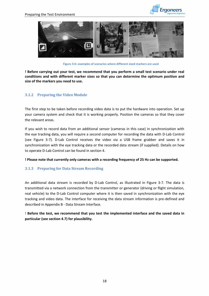
With D-Lab, several markers can be joined together (see section 5.1.9). This results in the ability to determine the position the AOIs more precisely. This is why it is recommended to position more than one marker near to an AOI. Depending on the size of the AOI, two to four or, if necessary, even six markers can be positioned, as shown in Figure 3-5.
Figure 3-5: positioning the markers for defining combined markers
Make sure that the resolution of the markers is large enough (Figure 3-3 shows examples of applications with different marker sizes). The size of the marker which is necessary for optimal detection is greatly influenced by the lighting conditions, the distance between the test person and the markers and the viewing angle.
Preparing the Test Environment
18
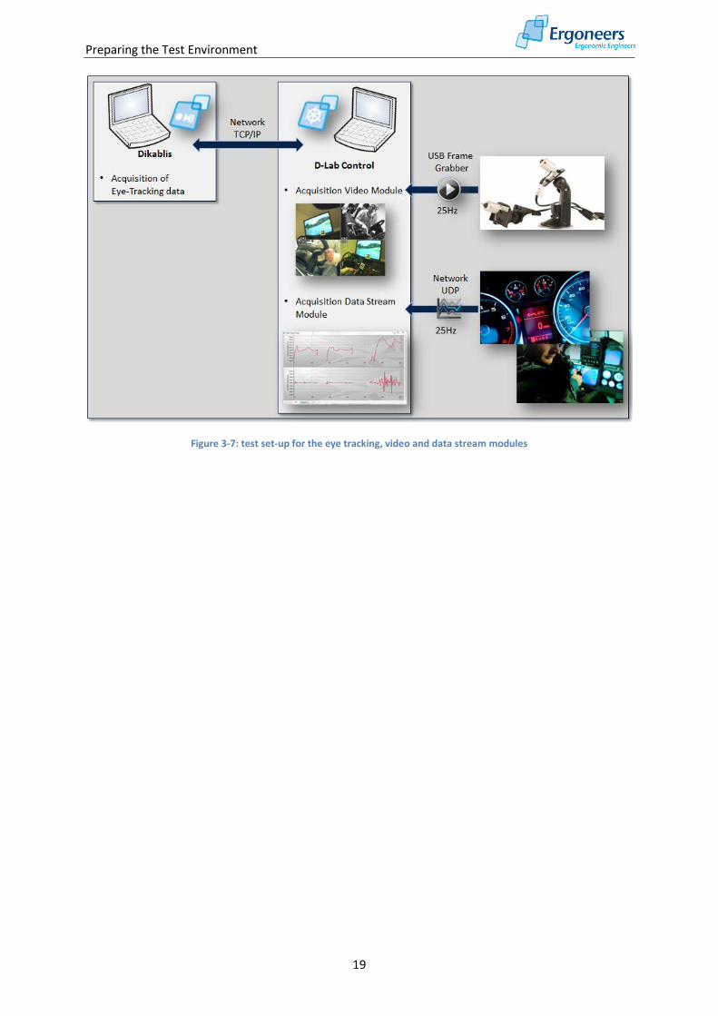
Figure 3-6: examples of scenarios where different sized markers are used
! Before carrying out your test, we recommend that you perform a small test scenario under real conditions and with different marker sizes so that you can determine the optimum position and size of the markers you need to use.
3.1.2 Preparing the Video Module
The first step to be taken before recording video data is to put the hardware into operation. Set up
your camera system and check that it is working properly. Position the cameras so that they cover
the relevant areas.
If you wish to record data from an additional sensor (cameras in this case) in synchronization with
the eye tracking data, you will require a second computer for recording the data with D-Lab Control
(see Figure 3-7). D-Lab Control receives the video via a USB frame grabber and saves it in
synchronization with the eye tracking data or the recorded data stream (if supplied). Details on how
to operate D-Lab Control can be found in section 4.
! Please note that currently only cameras with a recording frequency of 25 Hz can be supported.
3.1.3 Preparing for Data Stream Recording
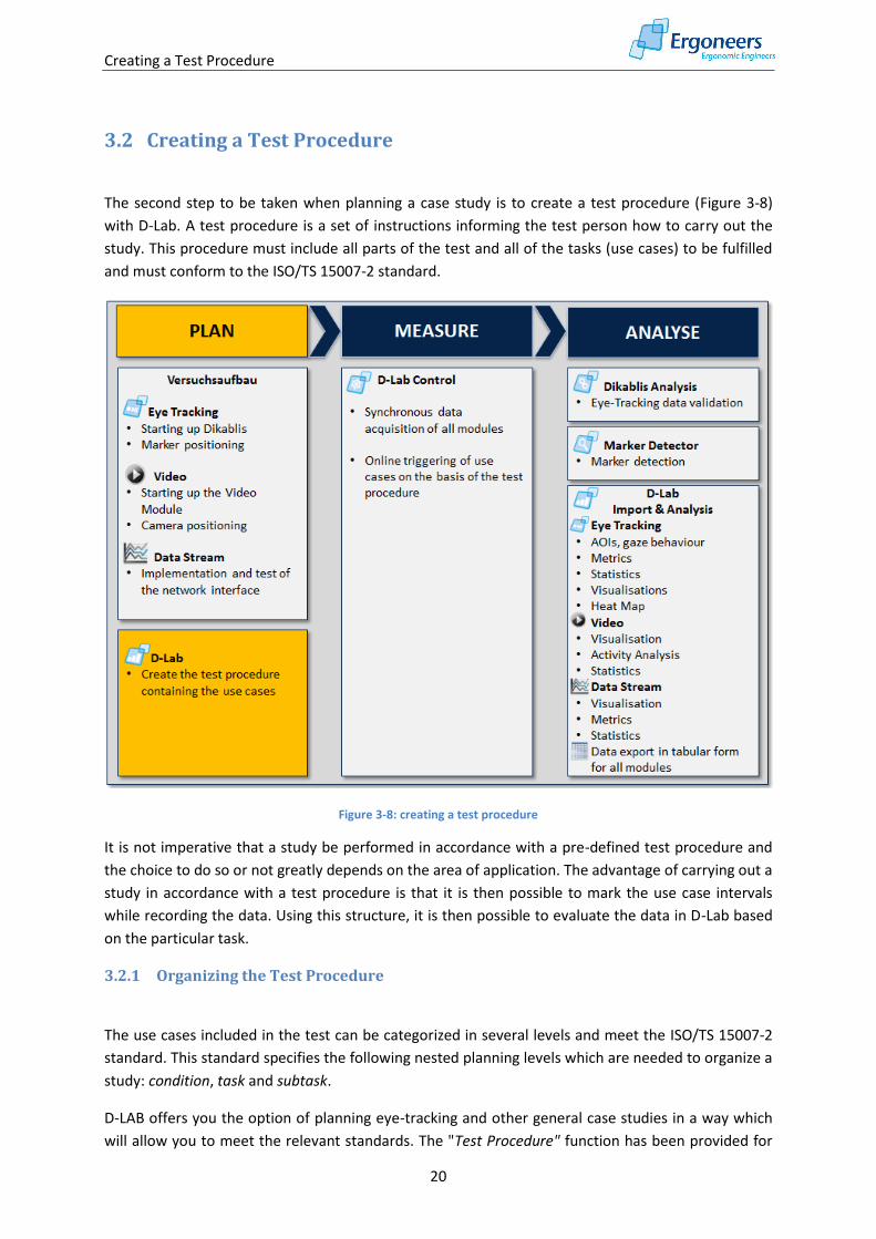
An additional data stream is recorded by D-Lab Control, as illustrated in Figure 3-7. The data is
transmitted via a network connection from the transmitter or generator (driving or flight simulation,
real vehicle) to the D-Lab Control computer where it is then saved in synchronization with the eye
tracking and video data. The interface for receiving the data stream information is pre-defined and
described in Appendix B - Data Stream Interface.
! Before the test, we recommend that you test the implemented interface and the saved data in
particular (see section 4.7) for plausibility.
Preparing the Test Environment
19
Figure 3-7: test set-up for the eye tracking, video and data stream modules
Creating a Test Procedure
20
3.2 Creating a Test Procedure
The second step to be taken when planning a case study is to create a test procedure (Figure 3-8)
with D-Lab. A test procedure is a set of instructions informing the test person how to carry out the
study. This procedure must include all parts of the test and all of the tasks (use cases) to be fulfilled
and must conform to the ISO/TS 15007-2 standard.
Figure 3-8: creating a test procedure
It is not imperative that a study be performed in accordance with a pre-defined test procedure and
the choice to do so or not greatly depends on the area of application. The advantage of carrying out a
study in accordance with a test procedure is that it is then possible to mark the use case intervals
while recording the data. Using this structure, it is then possible to evaluate the data in D-Lab based
on the particular task.
3.2.1 Organizing the Test Procedure
The use cases included in the test can be categorized in several levels and meet the ISO/TS 15007-2
standard. This standard specifies the following nested planning levels which are needed to organize a
study: condition, task and subtask.
D-LAB offers you the option of planning eye-tracking and other general case studies in a way which
will allow you to meet the relevant standards. The "Test Procedure" function has been provided for
Creating a Test Procedure
21
this purpose. You can use it to plan and manage test procedures independently from the D-Lab
modules. The following planning levels are available:
Condition is the highest planning level and is used to define different test variants. Example: for comparing navigation systems from different manufacturers; for comparing two positioning options for a display in a vehicle, for comparing a number of different shelf arrangements in a supermarket.
Task defines a subtest within a test variant. Example: the task groups: navigation tasks, media tasks etc.
Subtask allows for a more detailed division of the tasks into subtasks. Example: within the navigation tasks, the subtasks: destination, destination from address book, quit destination, etc.
Subsubtask offers the option of splitting up the tasks even further if necessary. Example of a navigation destination entry: city, street, house number.
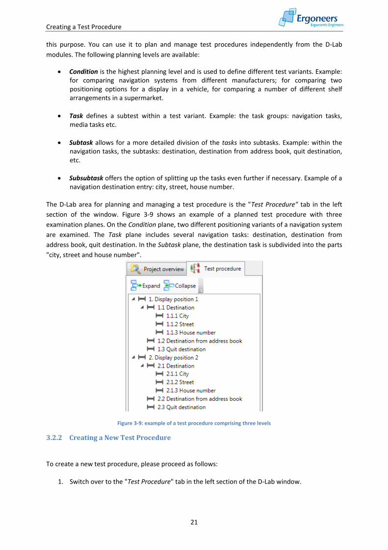
The D-Lab area for planning and managing a test procedure is the "Test Procedure" tab in the left
section of the window. Figure 3-9 shows an example of a planned test procedure with three
examination planes. On the Condition plane, two different positioning variants of a navigation system
are examined. The Task plane includes several navigation tasks: destination, destination from
address book, quit destination. In the Subtask plane, the destination task is subdivided into the parts
"city, street and house number".
Figure 3-9: example of a test procedure comprising three levels
3.2.2 Creating a New Test Procedure
To create a new test procedure, please proceed as follows:
1. Switch over to the "Test Procedure" tab in the left section of the D-Lab window.
Creating a Test Procedure
22
2. In the "Test Procedure" menu, select the entry "New" or click on the "New Test Procedure"
button in the D-Lab toolbar.
3. In the dialog which is then opened, select the directory in which you wish to save the test
procedure and enter a file name under which it should be saved. Press "Save" to create the
new test procedure.
4. An entry with the name "New Condition" will then be automatically saved in the "Test
Procedure" tab. The entry can be edited and you can enter whichever name you choose for
the first Condition of the procedure. Press the Enter button to end the editing procedure.
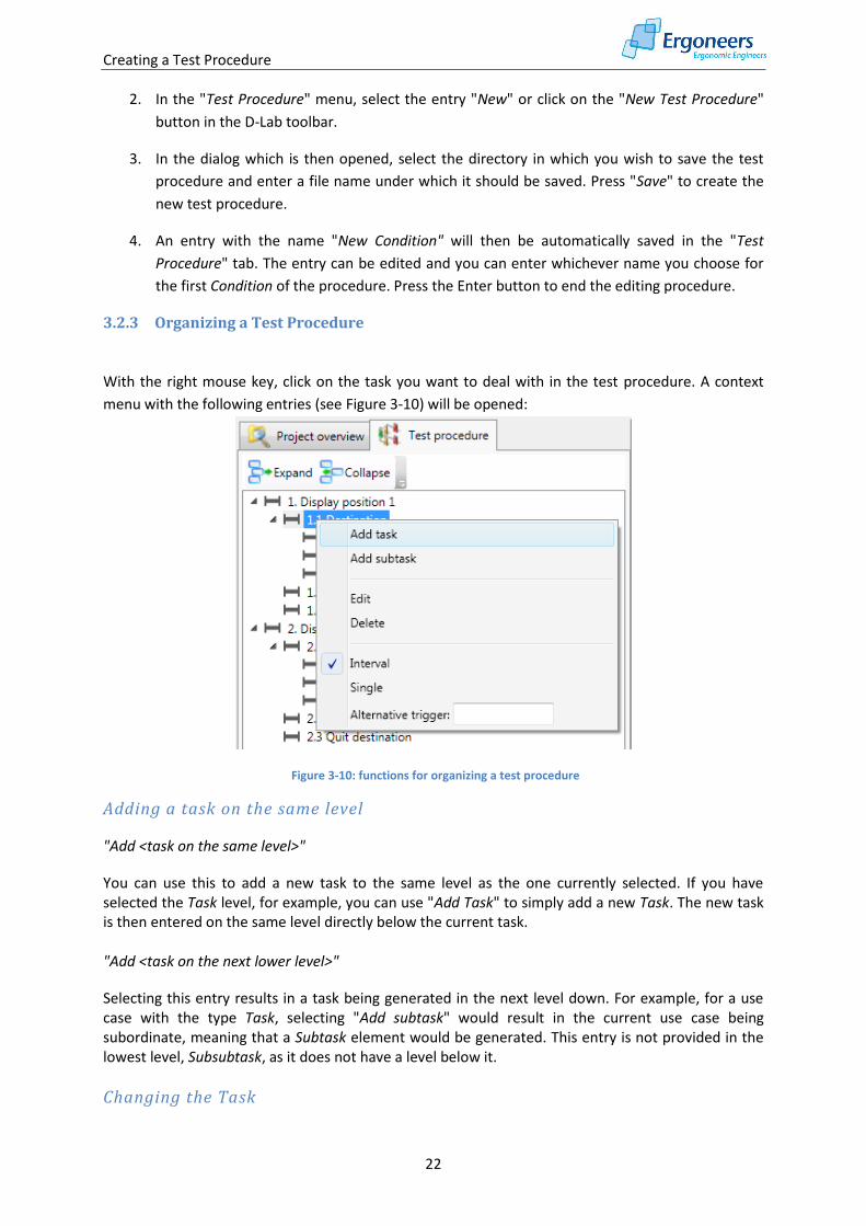
3.2.3 Organizing a Test Procedure
With the right mouse key, click on the task you want to deal with in the test procedure. A context
menu with the following entries (see Figure 3-10) will be opened:
Figure 3-10: functions for organizing a test procedure
Adding a task on the same level
"Add <task on the same level>"
You can use this to add a new task to the same level as the one currently selected. If you have selected the Task level, for example, you can use "Add Task" to simply add a new Task. The new task is then entered on the same level directly below the current task. "Add <task on the next lower level>"
Selecting this entry results in a task being generated in the next level down. For example, for a use case with the type Task, selecting "Add subtask" would result in the current use case being subordinate, meaning that a Subtask element would be generated. This entry is not provided in the lowest level, Subsubtask, as it does not have a level below it.
Changing the Task
Creating a Test Procedure
23
"Edit"
This option allows the name of the task to be changed. If you select this entry, the text field holding the name of the task can be edited by you. The editing process is completed by pressing "Enter".
Deleting the Task
"Delete"
If this entry is selected, the currently selected task and its subtasks will be deleted.
Determining the Task Type
“Interval" or "Single"
Each use case can either be an "interval use case" which is defined by a start and end time and takes
place over a specific period, or a single occurrence. "Interval" is the default type.
An example for an "Interval" use case type is the navigation destination entry. The pressing of a
button (for example, to change the radio transmitter) is an example of a "single" use case.
Remote Trigger Definition
"Alternative trigger”
This function can be used to assign an alias name (a so-called alternative trigger name) to the current use case. This "alternative trigger" name allows the remote-controlled triggering of use cases via the network by sending the defined alias to D-Lab Control. For a detailed description of this function, please consult Appendix A - D-Lab Control Network Interface.
3.2.4 Saving a Test Procedure
To save a test procedure:
1. Select the "Save" entry in the "Test Procedure" menu or click the "Save Test Procedure"
button in the D-LAB toolbar.
2. The test procedure is saved in the directory under the name you specified when you created
it.
! Please note that changes to a test procedure are not saved automatically. Therefore, please save any changes to the procedure manually before you shut down D-Lab or open a different test procedure.
3.2.5 Opening an Existing Test Procedure
To display and, if necessary, change an existing experiment procedure:
1. In the "Test Procedure" menu, select the entry "Open" or click on the "Open Test Procedure"
button in the D-Lab toolbar.
Creating a Test Procedure
24
2. In the window which is then opened, select the experiment procedure you would like to
open and click "Open".
3. The selected test procedure is then displayed in the "Test Procedure" tab.
Creating a Test Procedure
25
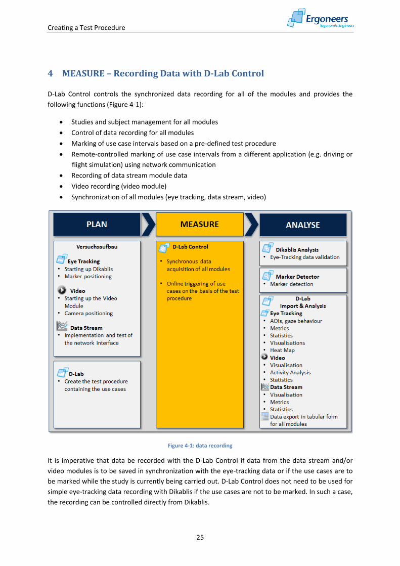
4 MEASURE – Recording Data with D-Lab Control D-Lab Control controls the synchronized data recording for all of the modules and provides the
following functions (Figure 4-1):
Studies and subject management for all modules
Control of data recording for all modules
Marking of use case intervals based on a pre-defined test procedure
Remote-controlled marking of use case intervals from a different application (e.g. driving or
flight simulation) using network communication
Recording of data stream module data
Video recording (video module)
Synchronization of all modules (eye tracking, data stream, video)
Figure 4-1: data recording
It is imperative that data be recorded with the D-Lab Control if data from the data stream and/or
video modules is to be saved in synchronization with the eye-tracking data or if the use cases are to
be marked while the study is currently being carried out. D-Lab Control does not need to be used for
simple eye-tracking data recording with Dikablis if the use cases are not to be marked. In such a case,
the recording can be controlled directly from Dikablis.
D-Lab Control - Modules and Structure
26
For an eye tracking study in which the use case intervals need to be marked in accordance with the
test procedure, D-Lab Control can be used parallel to the Dikablis Recorder on the Dikablis laptop. If
both the eye tracking data and other sensors are to be recorded (video or data stream), D-Lab
Control must be started on a separate computer. In such a case, D-Lab Control saves the data stream
and/or video data on the computer on which it is running and additionally records information for
synchronization with the eye-tracking data. The computers communicate via the network. A detailed
description of the interface used for the remote control of D-Lab Control (for controlling data
recording and marking use case intervals) can be found in Appendix A - D-Lab Control Network
Interface.
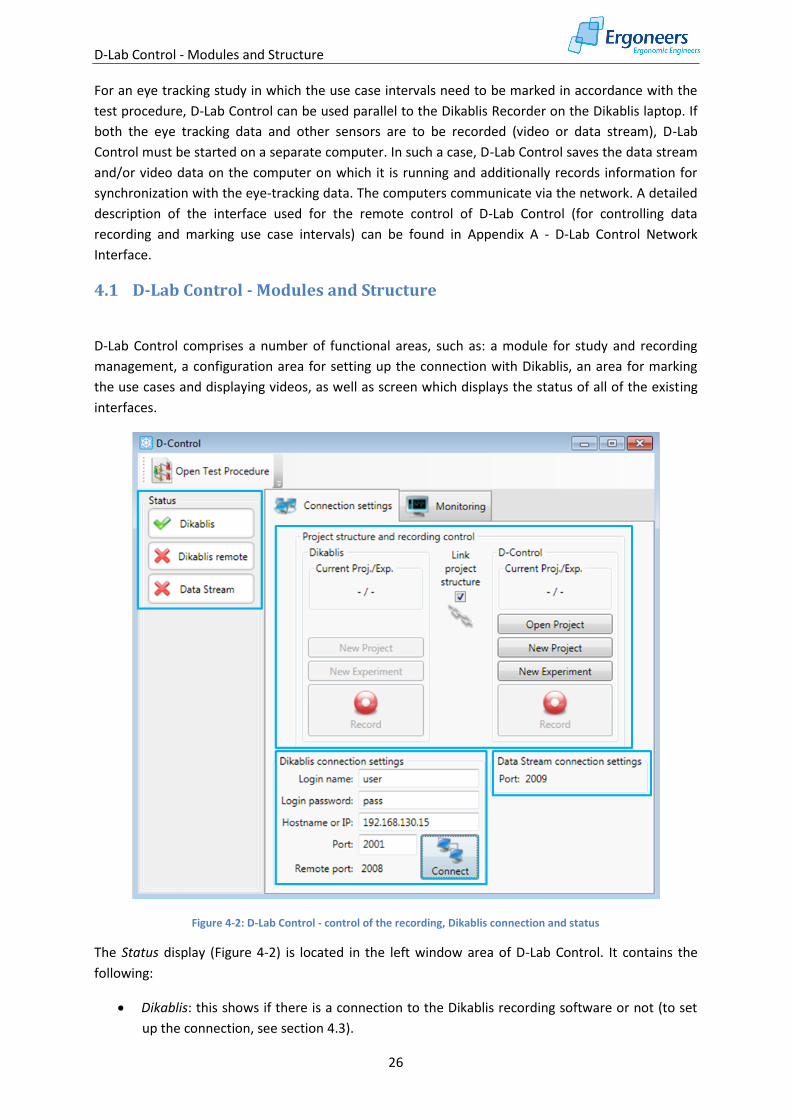
4.1 D-Lab Control - Modules and Structure
D-Lab Control comprises a number of functional areas, such as: a module for study and recording
management, a configuration area for setting up the connection with Dikablis, an area for marking
the use cases and displaying videos, as well as screen which displays the status of all of the existing
interfaces.
Figure 4-2: D-Lab Control - control of the recording, Dikablis connection and status
The Status display (Figure 4-2) is located in the left window area of D-Lab Control. It contains the
following:
Dikablis: this shows if there is a connection to the Dikablis recording software or not (to set
up the connection, see section 4.3).
Setting Up a Connection with the Video Module
27
Dikablis remote: indicates if a client has logged on via the network to operate the recording
by remote control or to mark the use cases (details on the interface for the remote control of
D-Lab Control can be found in Appendix A - D-Lab Control Network Interface).
Data Stream: this indicates if a client has been connected via the Data Stream interface
(details on the Data Stream interface can be found in Appendix B - Data Stream Interface).
A green check mark next to one of the above entries means that a connection has been set up with
the corresponding module/client. A red cross indicates that there is no connection.
The project and recording are managed in the "Project structure and recording control" area (Figure
4-2). Here, a new project can be created, an existing one can be continued and new test persons can
be added to the project. Furthermore, the data recording for all of the modules can be started and
stopped from this area.
The settings for connection to the Dikablis Recorder are listed under "Dikablis connection settings".
The settings for connection to the Data Stream interface are displayed in the "Data Stream
connection settings” area (Figure 4-2).
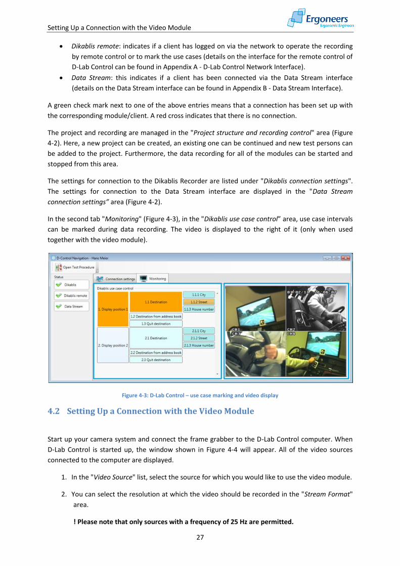
In the second tab "Monitoring" (Figure 4-3), in the "Dikablis use case control” area, use case intervals
can be marked during data recording. The video is displayed to the right of it (only when used
together with the video module).
Figure 4-3: D-Lab Control – use case marking and video display
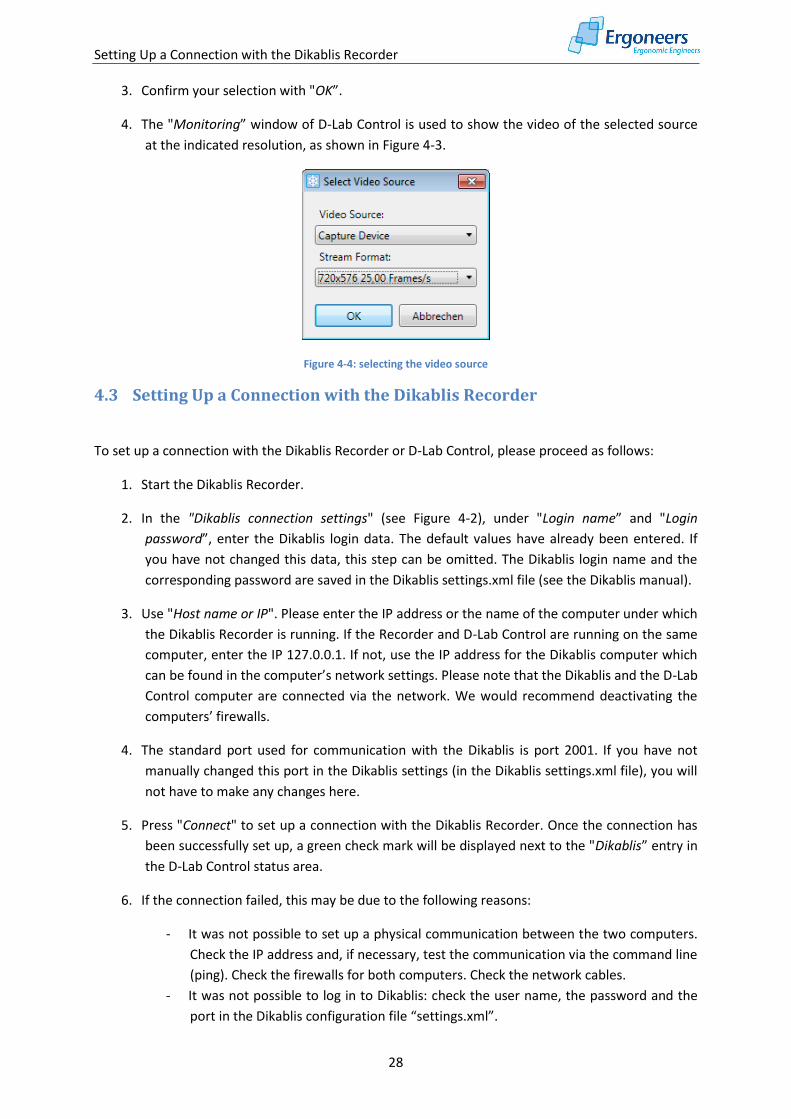
4.2 Setting Up a Connection with the Video Module
Start up your camera system and connect the frame grabber to the D-Lab Control computer. When
D-Lab Control is started up, the window shown in Figure 4-4 will appear. All of the video sources
connected to the computer are displayed.
1. In the "Video Source" list, select the source for which you would like to use the video module.
2. You can select the resolution at which the video should be recorded in the "Stream Format"
area.
! Please note that only sources with a frequency of 25 Hz are permitted.
Setting Up a Connection with the Dikablis Recorder
28
3. Confirm your selection with "OK”.
4. The "Monitoring” window of D-Lab Control is used to show the video of the selected source
at the indicated resolution, as shown in Figure 4-3.
Figure 4-4: selecting the video source
4.3 Setting Up a Connection with the Dikablis Recorder
To set up a connection with the Dikablis Recorder or D-Lab Control, please proceed as follows:
1. Start the Dikablis Recorder.
2. In the "Dikablis connection settings" (see Figure 4-2), under "Login name” and "Login
password”, enter the Dikablis login data. The default values have already been entered. If
you have not changed this data, this step can be omitted. The Dikablis login name and the
corresponding password are saved in the Dikablis settings.xml file (see the Dikablis manual).
3. Use "Host name or IP". Please enter the IP address or the name of the computer under which
the Dikablis Recorder is running. If the Recorder and D-Lab Control are running on the same
computer, enter the IP 127.0.0.1. If not, use the IP address for the Dikablis computer which
can be found in the computer’s network settings. Please note that the Dikablis and the D-Lab
Control computer are connected via the network. We would recommend deactivating the
computers’ firewalls.
4. The standard port used for communication with the Dikablis is port 2001. If you have not
manually changed this port in the Dikablis settings (in the Dikablis settings.xml file), you will
not have to make any changes here.
5. Press "Connect" to set up a connection with the Dikablis Recorder. Once the connection has
been successfully set up, a green check mark will be displayed next to the "Dikablis” entry in
the D-Lab Control status area.
6. If the connection failed, this may be due to the following reasons:
- It was not possible to set up a physical communication between the two computers.
Check the IP address and, if necessary, test the communication via the command line
(ping). Check the firewalls for both computers. Check the network cables.
- It was not possible to log in to Dikablis: check the user name, the password and the
port in the Dikablis configuration file “settings.xml”.
Setting Up a Connection with the Video Stream Module
29
- Only one connection can be set up with the Dikablis Recorder at one time. Please
check if a connection has already been set up in another D-Lab Control application or
instance.
4.4 Setting Up a Connection with the Video Stream Module
You do not need to take any action in D-Lab Control to set up a connection for receiving Data Stream
files. All you have to do is make sure that the network communication between the D-Lab Control
computer and the data stream transmitter is functioning properly. The data transmitter will set up
the connection. The interface for the Data Stream module is described in Appendix B - Data Stream
Interface. Once the source generating the data stream for D-Lab Control has logged in, a green check
mark will be displayed in the status area for "Data Stream" (Figure 4-3).
In the D-Lab Control area "Data Stream connection settings”, the port number used for
communicating (UDP) with the Data Stream module is displayed.
4.5 Setting Up the Dikablis Remote Connection
The Dikablis remote interface is used for the remote control of recording, project management and
use-case marking activities from another application via the network. The corresponding interface is
described in detail in Appendix A - D-Lab Control Network Interface.
As far as D-Lab Control is concerned, nothing needs to be done to set up the remote connection. It is
set up by the application which takes over the control. Once the application logs in to D-Lab Control
via the Dikablis remote interface, this is signaled through the appearance of a green check mark next
to the "Dikablis remote" entry (Figure 4-3).
The port number via which the connection is set up (UDP) is displayed in "Dikablis connection
settings" under "Remote port".
4.6 Study Management
In the "Project structure and recording control" area, you can find all of the functions needed to
generate projects and experiments and to control the data recordings for all of the modules (Figure
4-2).
In the left control group "Dikablis”, you can communicate directly with Dikablis to generate a project
or an experiment in the Dikablis Recorder or start/stop the recording of eye tracking data. The group
on the right, "D-Control" is for managing the study on the D-Lab Control computer. If there is a check
mark beside "Link project structure", the "D-Control" part will take over the control for both
components: Dikablis and D-Lab Control.
We recommend always ticking this box if you would like to record both eye tracking data and video
or data stream information. If only eye tracking data is recorded and you use D-Lab Control solely for
controlling Dikablis and marking use case intervals, you may remove the check mark and use the
control function in the "Dikablis" group.
Structure of the Data in D-Lab Control
30
4.7 Structure of the Data in D-Lab Control
As mentioned in section 4, D-Lab Control is used for recording the data from the Video and Data
Stream modules, among other things. This information is saved in synchronization with the eye
tracking data. To achieve this, the Dikablis data must be assigned to the D-Lab Control data. The
allocation is performed automatically in D-Lab Control due to the fact that there is only one single
controller for recording and managing projects and experiments. This is the case if the "Link project
structure" option is active and results in the following:
If a project is created, it is generated both on the Dikablis computer and on the D-Lab Control
computer. The data for D-Lab Control projects is saved under "C:\Control Center". A
directory with the project name is created here.
The same happens if an experiment is generated. The result is that a new experiment with
the specified name is generated in the project directory in both the Dikablis Recorder and the
D-Lab Control computer.
The recording is started and stopped synchronously at both components – Dikablis and D-Lab
Control. Here, D-Lab Control saves the data as follows:
- For each module, a folder is generated in the directory for the current test person:
the directories are named "Dikablis", "ADTF" and "ExternalVideo".
- Information regarding synchronization with Dikalis is saved in the "Dikablis"
directory.
- The received data stream data is saved in the "ADTF" directory.
- The recorded video is saved in the "ExternalVideo" folder. To prevent the video from
becoming too large, a cut is made every 15 minutes.
If the "Link project structure" option is inactive, Dikablis and D-Lab Control can be managed
independently from one another. Generally speaking, this is advantageous if only eye tracking data is
recorded. In such a case, D-Lab Control does not record any data meaning that it also does not
require a project. Use the Dikablis controller to manage eye-tracking data recording.
How to operate the system if the "Link project structure" option is active is described in the
following. The function can be analogously transferred to the Dikablis operation if the option is
inactive. The only difference is that without the "Link project structure” option only Dikablis can be
controlled.
4.8 Creating a New Project (Study)
To create a new project, proceed as follows:
1. In the "Project structure and recording control" area, select “New Project”.
2. In the dialog window which is subsequently opened, enter the project name beside "Project
name”, as shown in Figure 4-5.
3. Tick the box beside "Create a new experiment" if you wish to generate a new experiment and
enter the desired name beside "Experiment name”.
4. Select "Ok" to create the project (and, if required, also the experiment).
Creating a New Experiment (Subject)
31
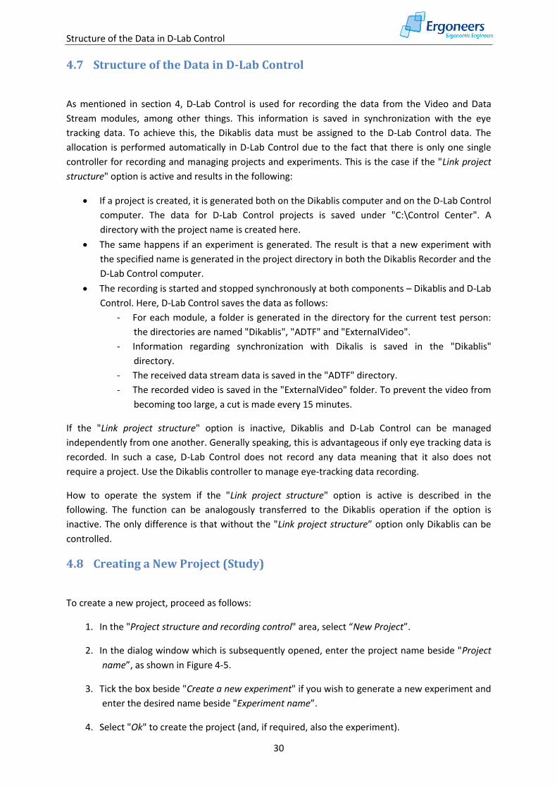
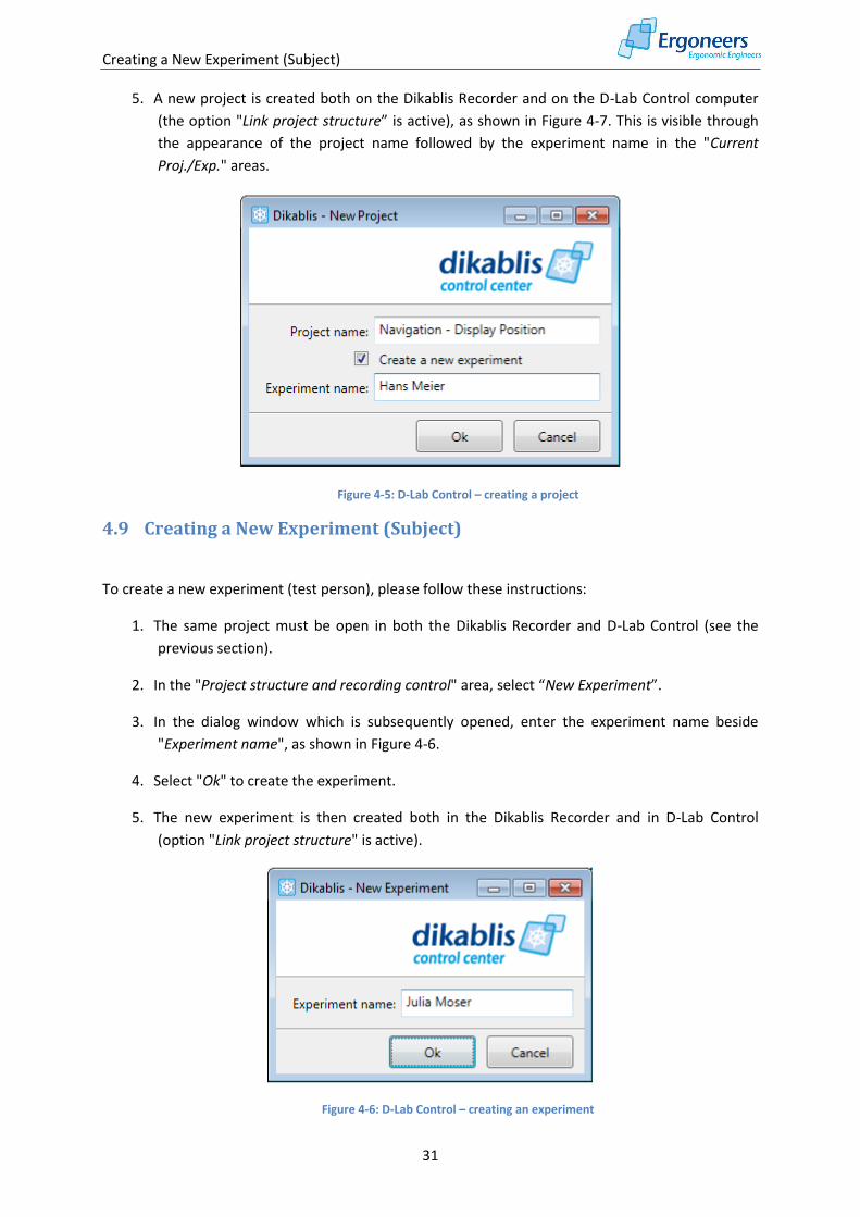
5. A new project is created both on the Dikablis Recorder and on the D-Lab Control computer
(the option "Link project structure” is active), as shown in Figure 4-7. This is visible through
the appearance of the project name followed by the experiment name in the "Current
Proj./Exp." areas.
Figure 4-5: D-Lab Control – creating a project
4.9 Creating a New Experiment (Subject)
To create a new experiment (test person), please follow these instructions:
1. The same project must be open in both the Dikablis Recorder and D-Lab Control (see the
previous section).
2. In the "Project structure and recording control" area, select “New Experiment”.
3. In the dialog window which is subsequently opened, enter the experiment name beside
"Experiment name", as shown in Figure 4-6.
4. Select "Ok" to create the experiment.
5. The new experiment is then created both in the Dikablis Recorder and in D-Lab Control
(option "Link project structure" is active).
Figure 4-6: D-Lab Control – creating an experiment
Opening a Project
32
Figure 4-7: D-Lab Control when it is ready to record
4.10 Opening a Project
Should you wish to continue working on an existing project, the project in question must firstly be
open. Currently it is not yet possible to open a Dikablis project via a network. The "Open Project"
button can only be used for local D-Lab Control projects. Dikablis projects must be opened manually
in the recording software. To open a project in D-Lab Control, proceed as follows:
1. Open the required project in the Dikablis recording software.
2. In D-Lab Control, press the "Open Project" button in the "Project structure and recording
control" area.
3. In the dialog which is subsequently opened, navigate to "C:\Control Center" and select the
project to be opened. You should select the same project as the one already open in the
Dikablis Recorder.
4. Select "Ok" to open the required project.
You can now create an experiment (as described in section 4.9) and start recording data.
4.11 Recording Data
To start recording data, the same project and experiment must be open in both applications (Dikablis
Recorder and D-Lab Control). "Link project structure" must be active.
1. Press the “Record" button to start recording for all connected modules. This will lead to
Dikablis starting the recording of eye tracking data. D-Lab Control will simultaneously start
saving the data from the video and Data Stream modules. In addition, information for the
Opening a Test Procedure
33
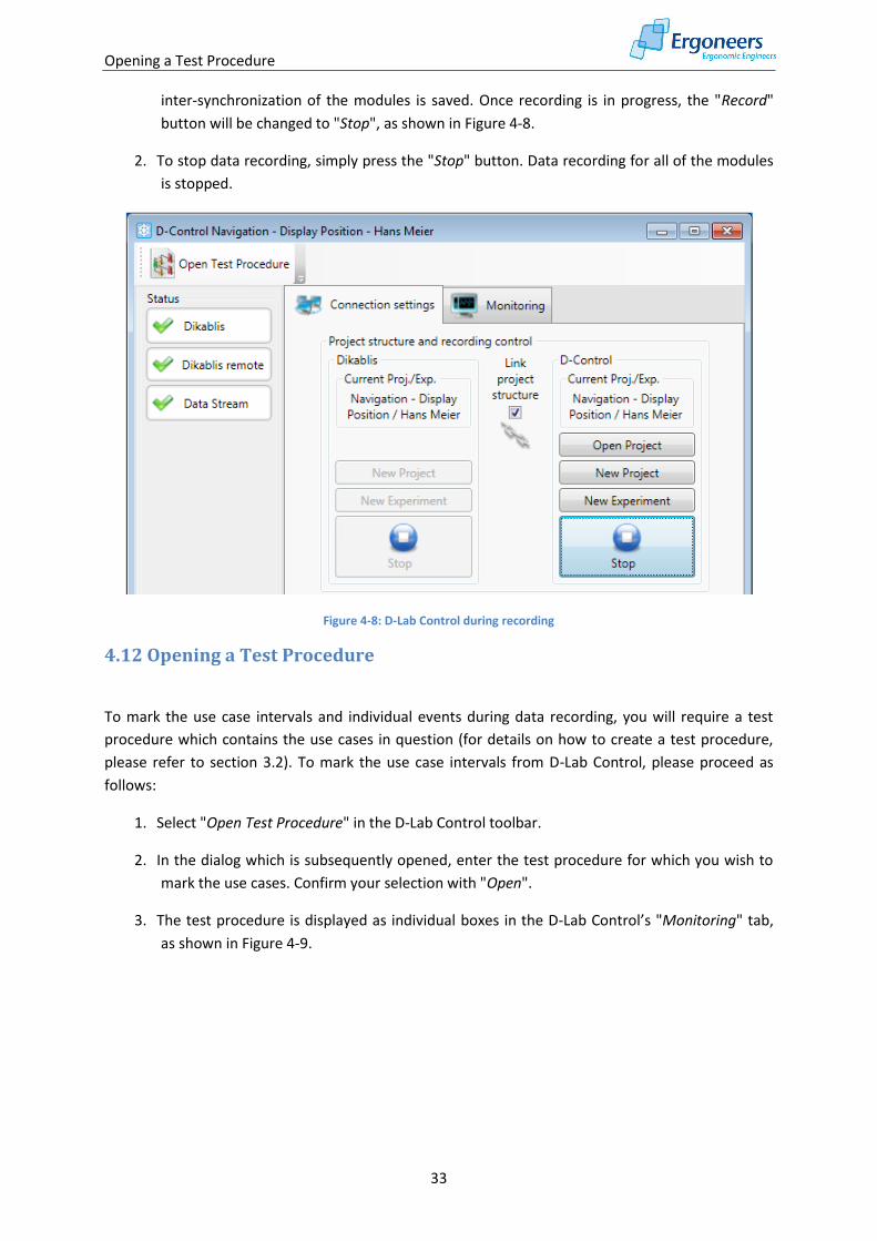
inter-synchronization of the modules is saved. Once recording is in progress, the "Record"
button will be changed to "Stop", as shown in Figure 4-8.
2. To stop data recording, simply press the "Stop" button. Data recording for all of the modules
is stopped.
Figure 4-8: D-Lab Control during recording
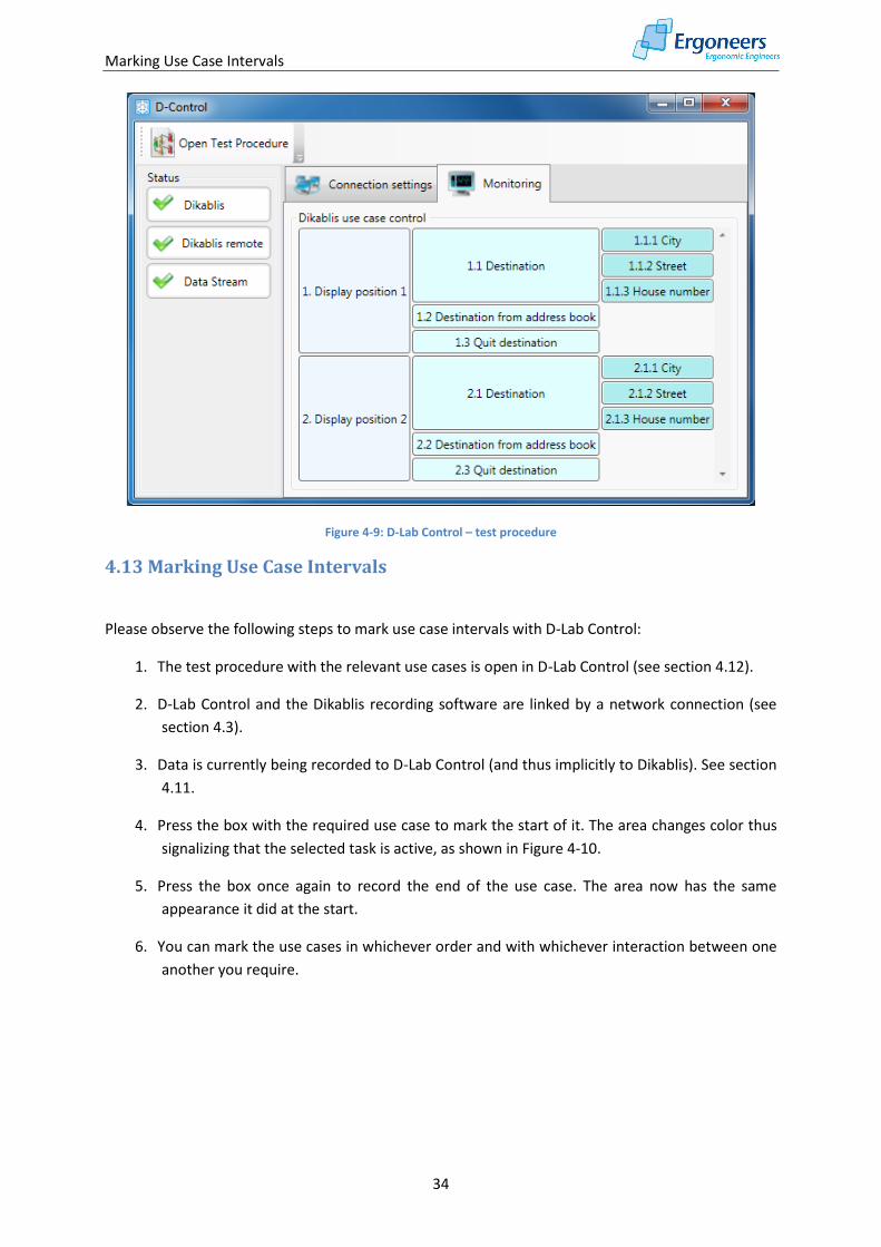
4.12 Opening a Test Procedure
To mark the use case intervals and individual events during data recording, you will require a test
procedure which contains the use cases in question (for details on how to create a test procedure,
please refer to section 3.2). To mark the use case intervals from D-Lab Control, please proceed as
follows:
1. Select "Open Test Procedure" in the D-Lab Control toolbar.
2. In the dialog which is subsequently opened, enter the test procedure for which you wish to
mark the use cases. Confirm your selection with "Open".
3. The test procedure is displayed as individual boxes in the D-Lab Control’s "Monitoring" tab,
as shown in Figure 4-9.
Marking Use Case Intervals
34
Figure 4-9: D-Lab Control – test procedure
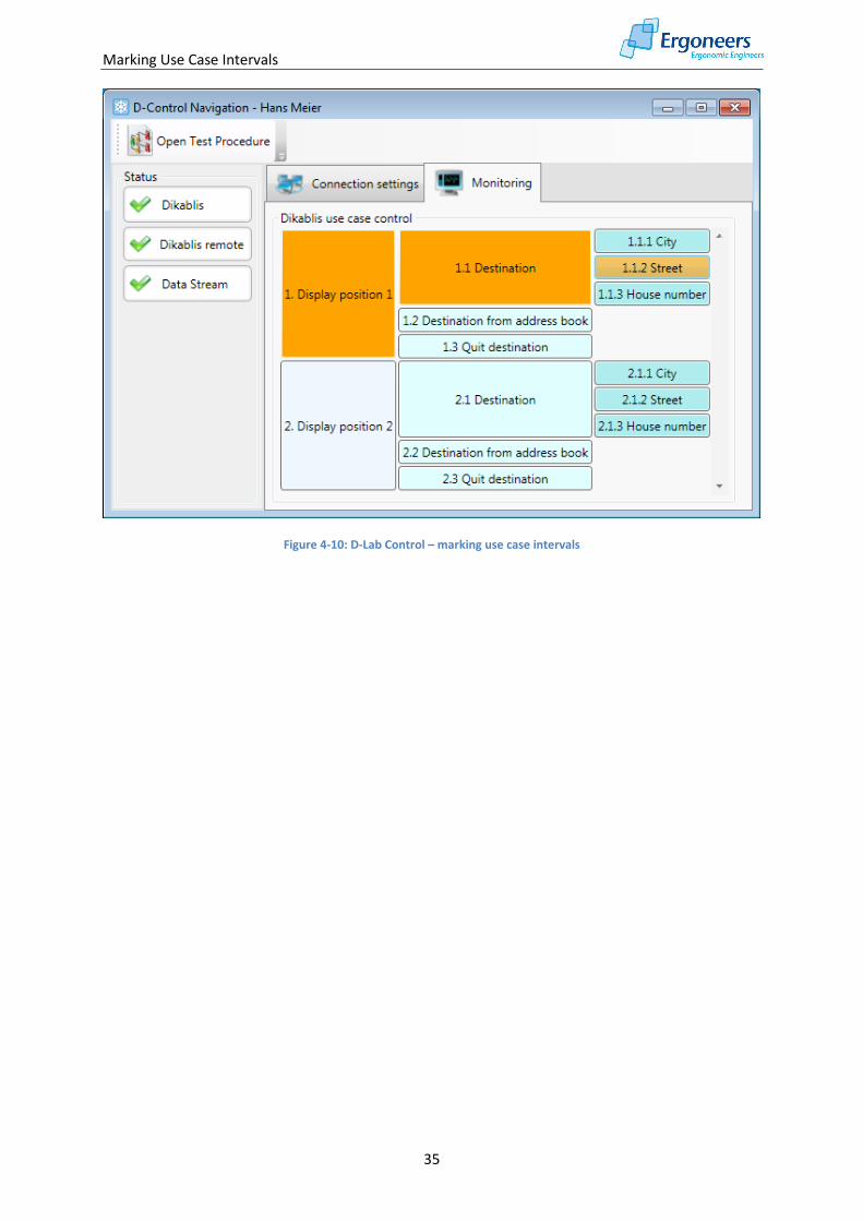
4.13 Marking Use Case Intervals
Please observe the following steps to mark use case intervals with D-Lab Control:
1. The test procedure with the relevant use cases is open in D-Lab Control (see section 4.12).
2. D-Lab Control and the Dikablis recording software are linked by a network connection (see
section 4.3).
3. Data is currently being recorded to D-Lab Control (and thus implicitly to Dikablis). See section
4.11.
4. Press the box with the required use case to mark the start of it. The area changes color thus
signalizing that the selected task is active, as shown in Figure 4-10.
5. Press the box once again to record the end of the use case. The area now has the same
appearance it did at the start.
6. You can mark the use cases in whichever order and with whichever interaction between one
another you require.
Marking Use Case Intervals
35
Figure 4-10: D-Lab Control – marking use case intervals
Eye Tracking Module
36
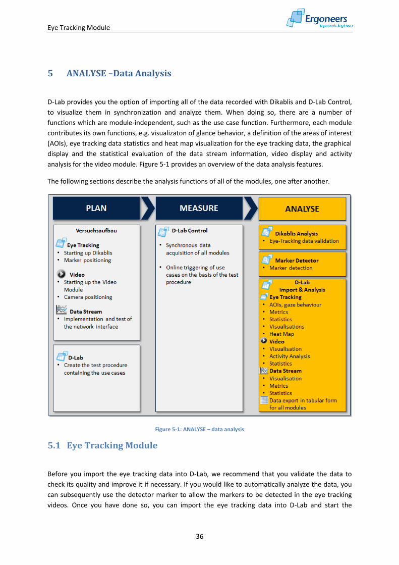
5 ANALYSE –Data Analysis
D-Lab provides you the option of importing all of the data recorded with Dikablis and D-Lab Control,
to visualize them in synchronization and analyze them. When doing so, there are a number of
functions which are module-independent, such as the use case function. Furthermore, each module
contributes its own functions, e.g. visualizaton of glance behavior, a definition of the areas of interest
(AOIs), eye tracking data statistics and heat map visualization for the eye tracking data, the graphical
display and the statistical evaluation of the data stream information, video display and activity
analysis for the video module. Figure 5-1 provides an overview of the data analysis features.
The following sections describe the analysis functions of all of the modules, one after another.
Figure 5-1: ANALYSE – data analysis
5.1 Eye Tracking Module
Before you import the eye tracking data into D-Lab, we recommend that you validate the data to
check its quality and improve it if necessary. If you would like to automatically analyze the data, you
can subsequently use the detector marker to allow the markers to be detected in the eye tracking
videos. Once you have done so, you can import the eye tracking data into D-Lab and start the
Eye Tracking Module
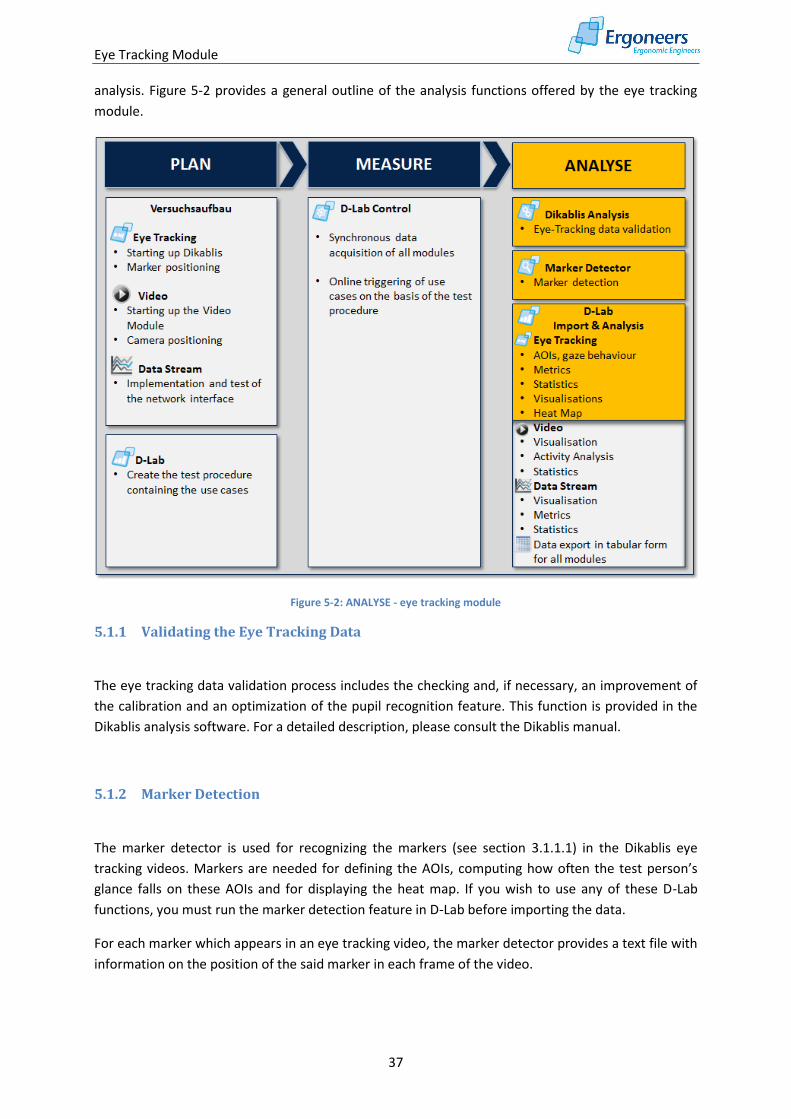
37
analysis. Figure 5-2 provides a general outline of the analysis functions offered by the eye tracking
module.
Figure 5-2: ANALYSE - eye tracking module
5.1.1 Validating the Eye Tracking Data
The eye tracking data validation process includes the checking and, if necessary, an improvement of
the calibration and an optimization of the pupil recognition feature. This function is provided in the
Dikablis analysis software. For a detailed description, please consult the Dikablis manual.
5.1.2 Marker Detection
The marker detector is used for recognizing the markers (see section 3.1.1.1) in the Dikablis eye
tracking videos. Markers are needed for defining the AOIs, computing how often the test person’s
glance falls on these AOIs and for displaying the heat map. If you wish to use any of these D-Lab
functions, you must run the marker detection feature in D-Lab before importing the data.
For each marker which appears in an eye tracking video, the marker detector provides a text file with
information on the position of the said marker in each frame of the video.
Eye Tracking Module
38
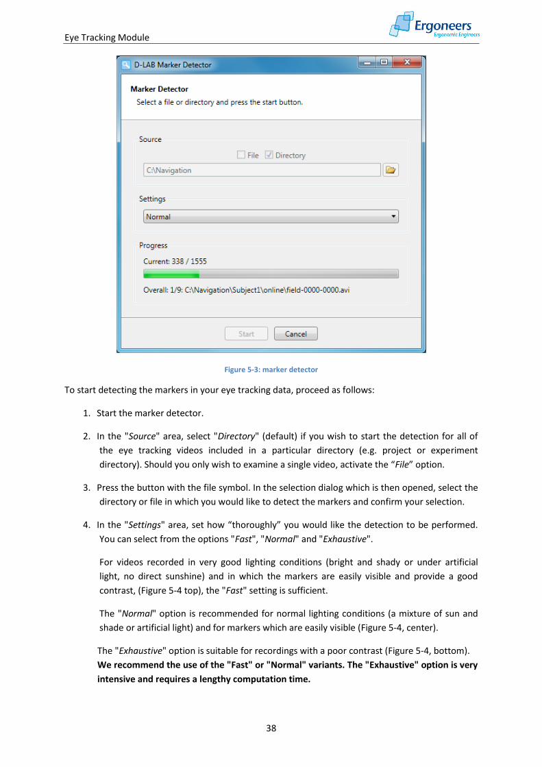
Figure 5-3: marker detector
To start detecting the markers in your eye tracking data, proceed as follows:
1. Start the marker detector.
2. In the "Source" area, select "Directory" (default) if you wish to start the detection for all of
the eye tracking videos included in a particular directory (e.g. project or experiment
directory). Should you only wish to examine a single video, activate the “File” option.
3. Press the button with the file symbol. In the selection dialog which is then opened, select the
directory or file in which you would like to detect the markers and confirm your selection.
4. In the "Settings" area, set how “thoroughly” you would like the detection to be performed.
You can select from the options "Fast", "Normal" and "Exhaustive".
For videos recorded in very good lighting conditions (bright and shady or under artificial
light, no direct sunshine) and in which the markers are easily visible and provide a good
contrast, (Figure 5-4 top), the "Fast" setting is sufficient.
The "Normal" option is recommended for normal lighting conditions (a mixture of sun and
shade or artificial light) and for markers which are easily visible (Figure 5-4, center).
The "Exhaustive" option is suitable for recordings with a poor contrast (Figure 5-4, bottom).
We recommend the use of the "Fast" or "Normal" variants. The "Exhaustive" option is very
intensive and requires a lengthy computation time.
Eye Tracking Module
39
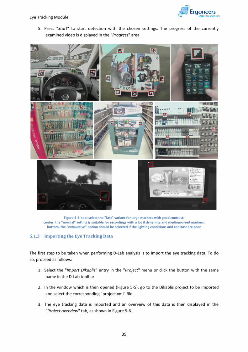
5. Press "Start" to start detection with the chosen settings. The progress of the currently
examined video is displayed in the "Progress" area.
Figure 5-4: top: select the "fast" variant for large markers with good contrast: center, the “normal” setting is suitable for recordings with a lot if dynamics and medium-sized markers:
bottom, the "exhaustive" option should be selected if the lighting conditions and contrast are poor
5.1.3 Importing the Eye Tracking Data
The first step to be taken when performing D-Lab analysis is to import the eye tracking data. To do
so, proceed as follows:
1. Select the "Import Dikablis" entry in the "Project" menu or click the button with the same
name in the D-Lab toolbar.
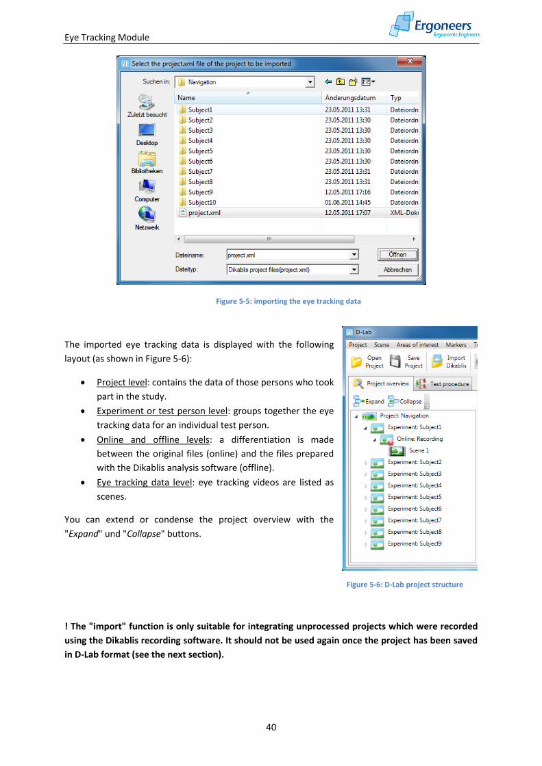
2. In the window which is then opened (Figure 5-5), go to the Dikablis project to be imported
and select the corresponding "project.xml" file.
3. The eye tracking data is imported and an overview of this data is then displayed in the
"Project overview" tab, as shown in Figure 5-6.
Eye Tracking Module
40
Figure 5-5: importing the eye tracking data
The imported eye tracking data is displayed with the following
layout (as shown in Figure 5-6):
Project level: contains the data of those persons who took
part in the study.
Experiment or test person level: groups together the eye
tracking data for an individual test person.
Online and offline levels: a differentiation is made
between the original files (online) and the files prepared
with the Dikablis analysis software (offline).
Eye tracking data level: eye tracking videos are listed as
scenes.
You can extend or condense the project overview with the
"Expand" und "Collapse" buttons.
! The "import" function is only suitable for integrating unprocessed projects which were recorded
using the Dikablis recording software. It should not be used again once the project has been saved
in D-Lab format (see the next section).
Figure 5-6: D-Lab project structure
Eye Tracking Module
41
5.1.4 Saving a Project
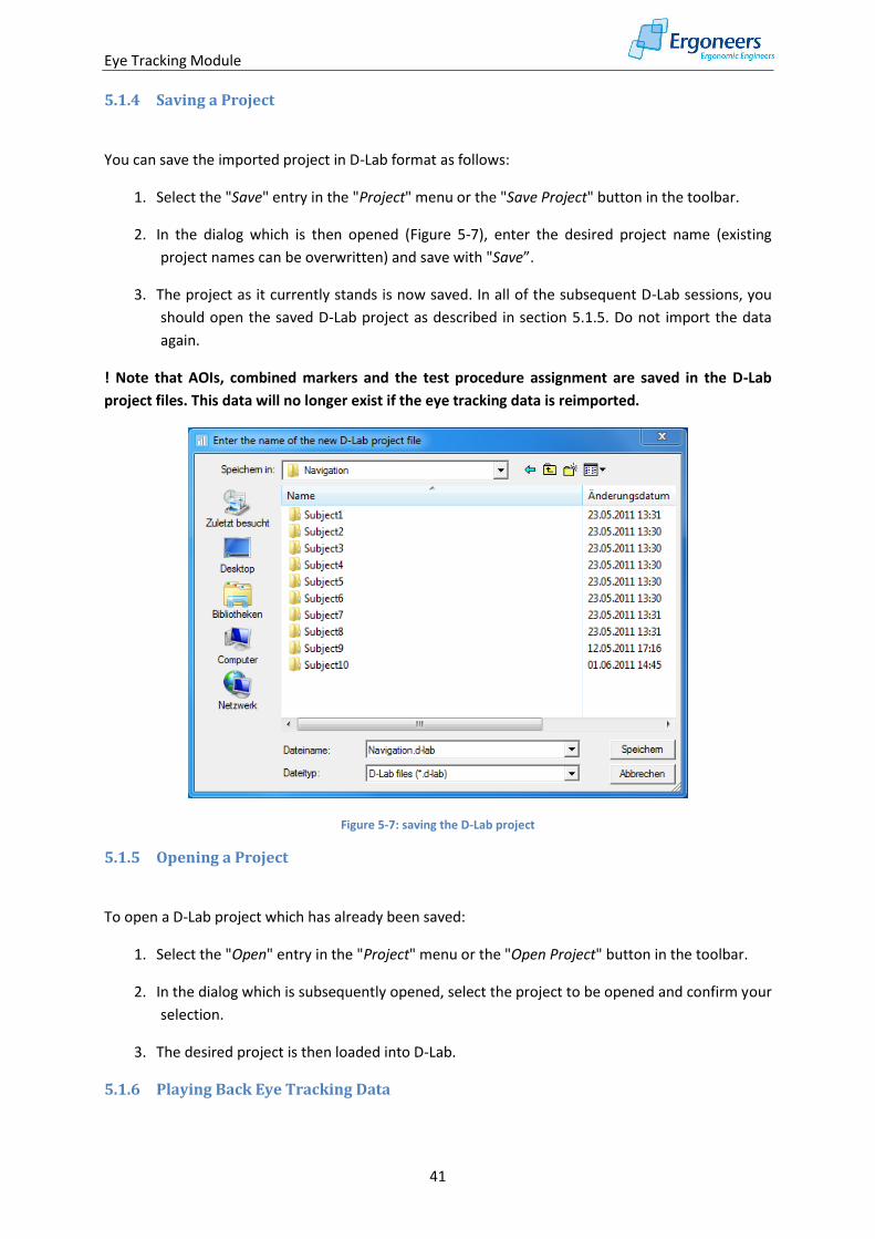
You can save the imported project in D-Lab format as follows:
1. Select the "Save" entry in the "Project" menu or the "Save Project" button in the toolbar.
2. In the dialog which is then opened (Figure 5-7), enter the desired project name (existing
project names can be overwritten) and save with "Save”.
3. The project as it currently stands is now saved. In all of the subsequent D-Lab sessions, you
should open the saved D-Lab project as described in section 5.1.5. Do not import the data
again.
! Note that AOIs, combined markers and the test procedure assignment are saved in the D-Lab
project files. This data will no longer exist if the eye tracking data is reimported.
Figure 5-7: saving the D-Lab project
5.1.5 Opening a Project
To open a D-Lab project which has already been saved:
1. Select the "Open" entry in the "Project" menu or the "Open Project" button in the toolbar.
2. In the dialog which is subsequently opened, select the project to be opened and confirm your
selection.
3. The desired project is then loaded into D-Lab.
5.1.6 Playing Back Eye Tracking Data
Eye Tracking Module
42
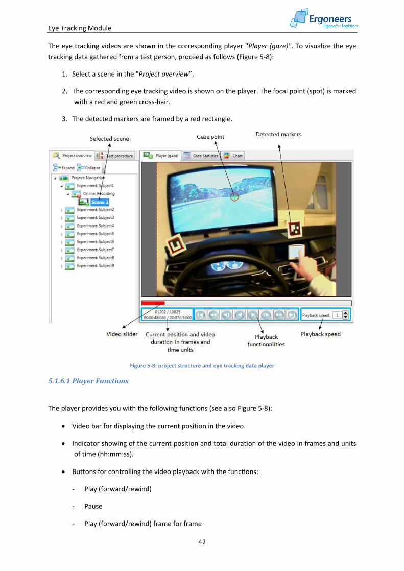
The eye tracking videos are shown in the corresponding player "Player (gaze)". To visualize the eye
tracking data gathered from a test person, proceed as follows (Figure 5-8):
1. Select a scene in the "Project overview”.
2. The corresponding eye tracking video is shown on the player. The focal point (spot) is marked
with a red and green cross-hair.
3. The detected markers are framed by a red rectangle.
Figure 5-8: project structure and eye tracking data player
5.1.6.1 Player Functions
The player provides you with the following functions (see also Figure 5-8):
Video bar for displaying the current position in the video.
Indicator showing of the current position and total duration of the video in frames and units
of time (hh:mm:ss).
Buttons for controlling the video playback with the functions:
- Play (forward/rewind)
- Pause
- Play (forward/rewind) frame for frame
Eye Tracking Module
43
- Play (forward/rewind) in 1 second intervals
- Jump to the start of the video
- Jump to the end of the video
Set the play speed - it is possible to play the video at two, five or ten times the speed, or in
slow motion.
To navigate quickly through the video, move the mouse cursor over the video bar and use
drag & drop to pull the video to the required position.
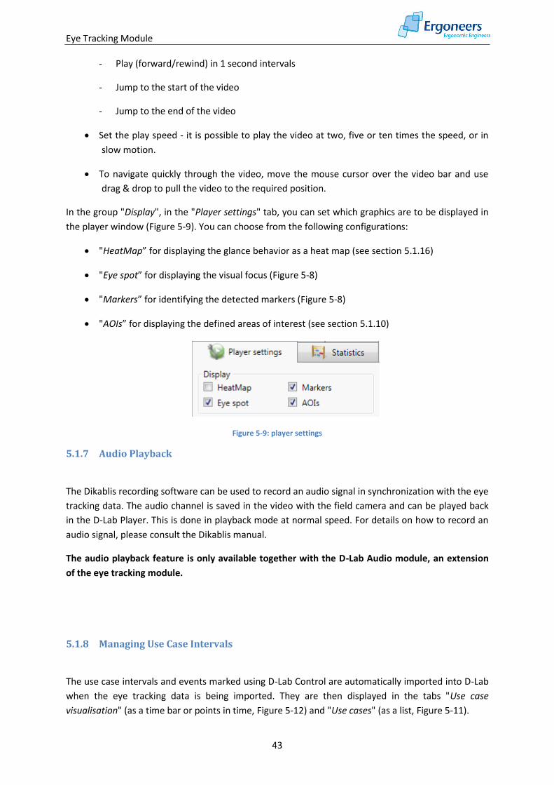
In the group "Display", in the "Player settings" tab, you can set which graphics are to be displayed in
the player window (Figure 5-9). You can choose from the following configurations:
"HeatMap” for displaying the glance behavior as a heat map (see section 5.1.16)
"Eye spot” for displaying the visual focus (Figure 5-8)
"Markers” for identifying the detected markers (Figure 5-8)
"AOIs” for displaying the defined areas of interest (see section 5.1.10)
Figure 5-9: player settings
5.1.7 Audio Playback
The Dikablis recording software can be used to record an audio signal in synchronization with the eye
tracking data. The audio channel is saved in the video with the field camera and can be played back
in the D-Lab Player. This is done in playback mode at normal speed. For details on how to record an
audio signal, please consult the Dikablis manual.
The audio playback feature is only available together with the D-Lab Audio module, an extension
of the eye tracking module.
5.1.8 Managing Use Case Intervals
The use case intervals and events marked using D-Lab Control are automatically imported into D-Lab
when the eye tracking data is being imported. They are then displayed in the tabs "Use case
visualisation" (as a time bar or points in time, Figure 5-12) and "Use cases" (as a list, Figure 5-11).
Eye Tracking Module
44
5.1.8.1 Importing a Test Procedure
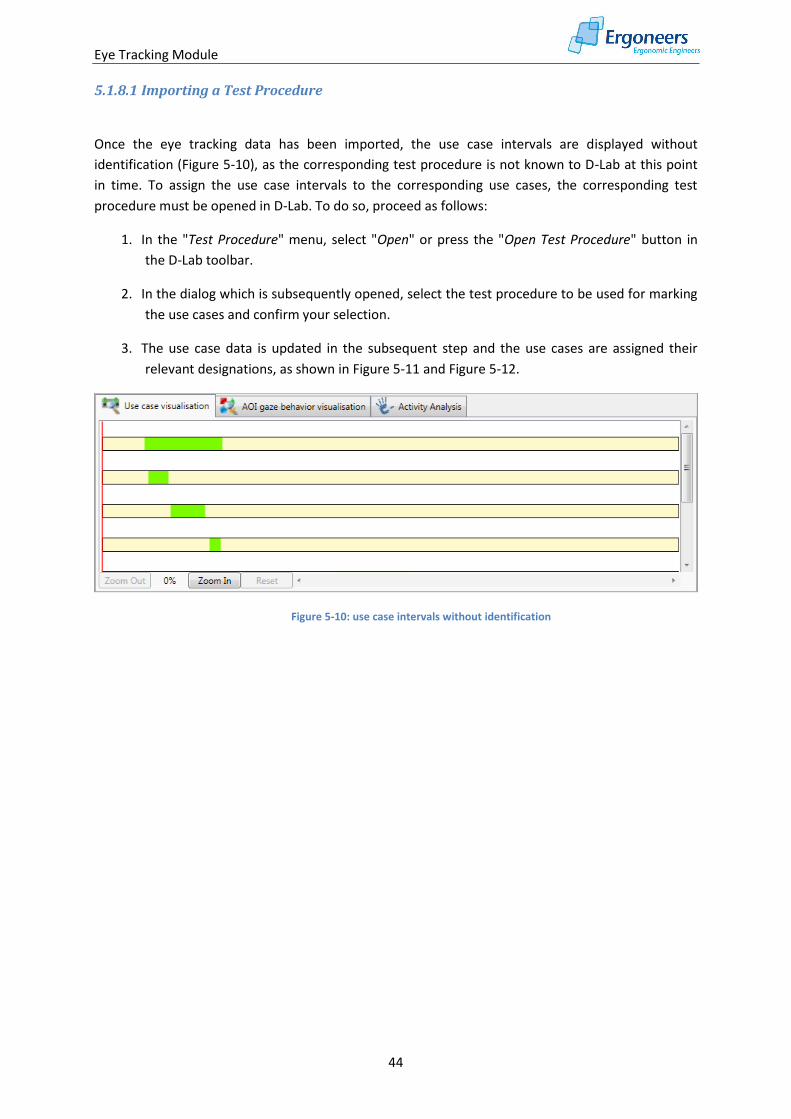
Once the eye tracking data has been imported, the use case intervals are displayed without
identification (Figure 5-10), as the corresponding test procedure is not known to D-Lab at this point
in time. To assign the use case intervals to the corresponding use cases, the corresponding test
procedure must be opened in D-Lab. To do so, proceed as follows:
1. In the "Test Procedure" menu, select "Open" or press the "Open Test Procedure" button in
the D-Lab toolbar.
2. In the dialog which is subsequently opened, select the test procedure to be used for marking
the use cases and confirm your selection.
3. The use case data is updated in the subsequent step and the use cases are assigned their
relevant designations, as shown in Figure 5-11 and Figure 5-12.
Figure 5-10: use case intervals without identification
Eye Tracking Module
45
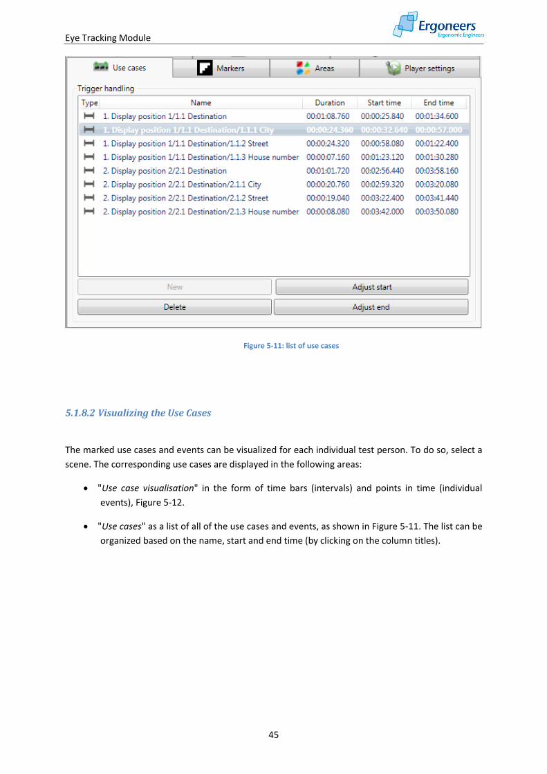
Figure 5-11: list of use cases
5.1.8.2 Visualizing the Use Cases
The marked use cases and events can be visualized for each individual test person. To do so, select a
scene. The corresponding use cases are displayed in the following areas:
"Use case visualisation" in the form of time bars (intervals) and points in time (individual
events), Figure 5-12.
"Use cases" as a list of all of the use cases and events, as shown in Figure 5-11. The list can be
organized based on the name, start and end time (by clicking on the column titles).
Eye Tracking Module
46
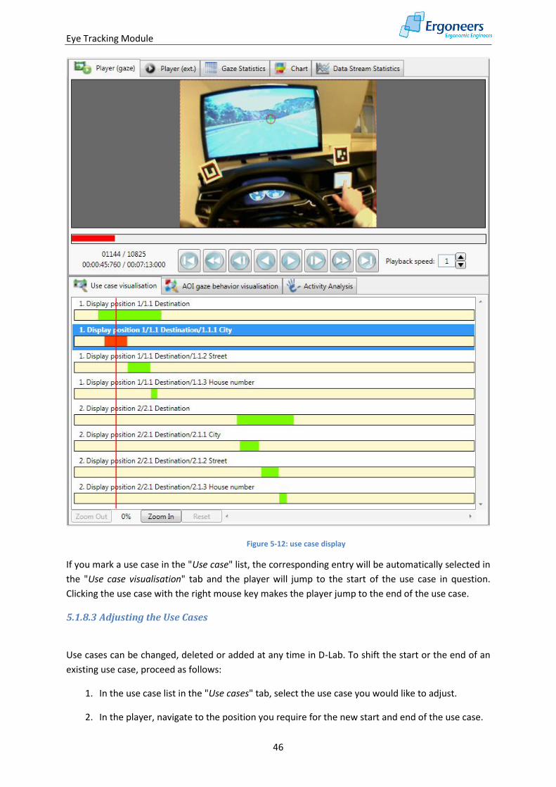
Figure 5-12: use case display
If you mark a use case in the "Use case" list, the corresponding entry will be automatically selected in
the "Use case visualisation" tab and the player will jump to the start of the use case in question.
Clicking the use case with the right mouse key makes the player jump to the end of the use case.
5.1.8.3 Adjusting the Use Cases
Use cases can be changed, deleted or added at any time in D-Lab. To shift the start or the end of an
existing use case, proceed as follows:
1. In the use case list in the "Use cases" tab, select the use case you would like to adjust.
2. In the player, navigate to the position you require for the new start and end of the use case.
Eye Tracking Module
47
3. Under "Use cases”, select the "Adjust start" button to set the start of the use case to the
current video position or "Adjust end" to move the end. To move individual events, you can
use both "Adjust start" and "Adjust end".
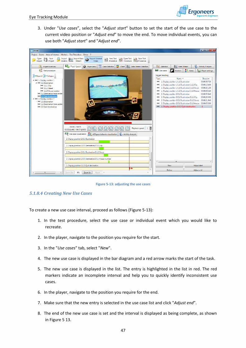
Figure 5-13: adjusting the use cases
5.1.8.4 Creating New Use Cases
To create a new use case interval, proceed as follows (Figure 5-13):
1. In the test procedure, select the use case or individual event which you would like to
recreate.
2. In the player, navigate to the position you require for the start.
3. In the "Use cases" tab, select "New".
4. The new use case is displayed in the bar diagram and a red arrow marks the start of the task.
5. The new use case is displayed in the list. The entry is highlighted in the list in red. The red
markers indicate an incomplete interval and help you to quickly identify inconsistent use
cases.
6. In the player, navigate to the position you require for the end.
7. Make sure that the new entry is selected in the use case list and click "Adjust end”.
8. The end of the new use case is set and the interval is displayed as being complete, as shown
in Figure 5 13.
Eye Tracking Module
48
5.1.8.5 Deleting Tasks
1. From the list, select the use case or the event you would like to delete.
2. Click the "Delete" button in the "Use case" tab to completely delete the use case.
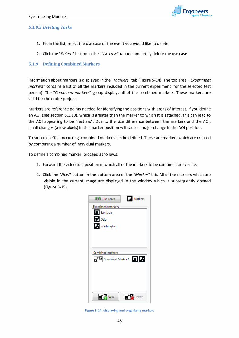
5.1.9 Defining Combined Markers
Information about markers is displayed in the "Markers" tab (Figure 5-14). The top area, "Experiment
markers" contains a list of all the markers included in the current experiment (for the selected test
person). The "Combined markers" group displays all of the combined markers. These markers are
valid for the entire project.
Markers are reference points needed for identifying the positions with areas of interest. If you define
an AOI (see section 5.1.10), which is greater than the marker to which it is attached, this can lead to
the AOI appearing to be "restless". Due to the size difference between the markers and the AOI,
small changes (a few pixels) in the marker position will cause a major change in the AOI position.
To stop this effect occurring, combined markers can be defined. These are markers which are created
by combining a number of individual markers.
To define a combined marker, proceed as follows:
1. Forward the video to a position in which all of the markers to be combined are visible.
2. Click the "New" button in the bottom area of the "Marker" tab. All of the markers which are
visible in the current image are displayed in the window which is subsequently opened
(Figure 5-15).
Figure 5-14: displaying and organizing markers
Eye Tracking Module
49
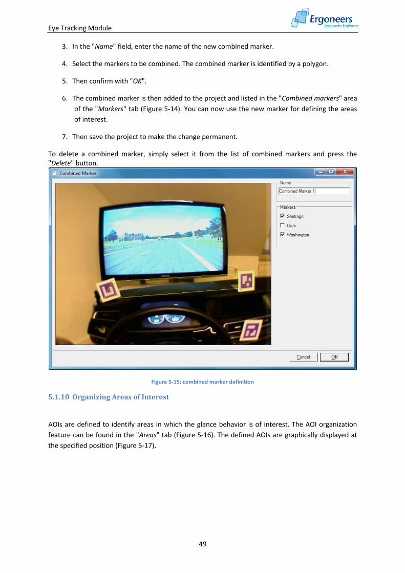
3. In the "Name" field, enter the name of the new combined marker.
4. Select the markers to be combined. The combined marker is identified by a polygon.
5. Then confirm with "OK".
6. The combined marker is then added to the project and listed in the "Combined markers" area
of the "Markers" tab (Figure 5-14). You can now use the new marker for defining the areas
of interest.
7. Then save the project to make the change permanent.
To delete a combined marker, simply select it from the list of combined markers and press the "Delete" button.
Figure 5-15: combined marker definition
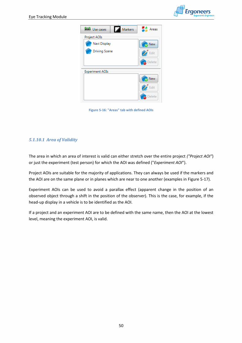
5.1.10 Organizing Areas of Interest
AOIs are defined to identify areas in which the glance behavior is of interest. The AOI organization
feature can be found in the "Areas" tab (Figure 5-16). The defined AOIs are graphically displayed at
the specified position (Figure 5-17).
Eye Tracking Module
50
Figure 5-16: "Areas" tab with defined AOIs
5.1.10.1 Area of Validity
The area in which an area of interest is valid can either stretch over the entire project ("Project AOI")
or just the experiment (test person) for which the AOI was defined ("Experiment AOI").
Project AOIs are suitable for the majority of applications. They can always be used if the markers and
the AOI are on the same plane or in planes which are near to one another (examples in Figure 5-17).
Experiment AOIs can be used to avoid a parallax effect (apparent change in the position of an
observed object through a shift in the position of the observer). This is the case, for example, if the
head-up display in a vehicle is to be identified as the AOI.
If a project and an experiment AOI are to be defined with the same name, then the AOI at the lowest
level, meaning the experiment AOI, is valid.
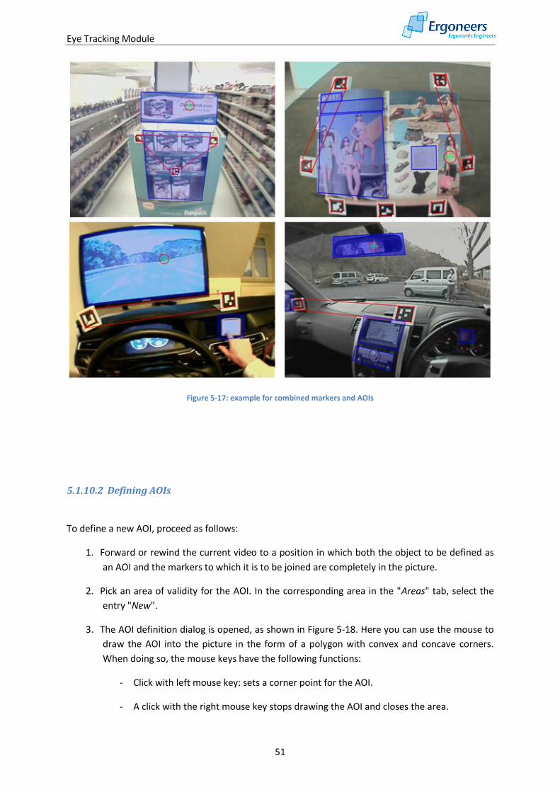
Eye Tracking Module
51
Figure 5-17: example for combined markers and AOIs
5.1.10.2 Defining AOIs
To define a new AOI, proceed as follows:
1. Forward or rewind the current video to a position in which both the object to be defined as
an AOI and the markers to which it is to be joined are completely in the picture.
2. Pick an area of validity for the AOI. In the corresponding area in the "Areas" tab, select the
entry "New".
3. The AOI definition dialog is opened, as shown in Figure 5-18. Here you can use the mouse to
draw the AOI into the picture in the form of a polygon with convex and concave corners.
When doing so, the mouse keys have the following functions:
- Click with left mouse key: sets a corner point for the AOI.
- A click with the right mouse key stops drawing the AOI and closes the area.
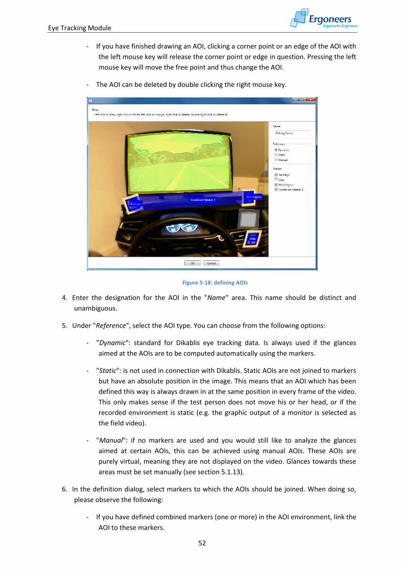
Eye Tracking Module
52
- If you have finished drawing an AOI, clicking a corner point or an edge of the AOI with
the left mouse key will release the corner point or edge in question. Pressing the left
mouse key will move the free point and thus change the AOI.
- The AOI can be deleted by double clicking the right mouse key.
Figure 5-18: defining AOIs
4. Enter the designation for the AOI in the "Name" area. This name should be distinct and
unambiguous.
5. Under "Reference", select the AOI type. You can choose from the following options:
- "Dynamic": standard for Dikablis eye tracking data. Is always used if the glances
aimed at the AOIs are to be computed automatically using the markers.
- "Static": is not used in connection with Dikablis. Static AOIs are not joined to markers
but have an absolute position in the image. This means that an AOI which has been
defined this way is always drawn in at the same position in every frame of the video.
This only makes sense if the test person does not move his or her head, or if the
recorded environment is static (e.g. the graphic output of a monitor is selected as
the field video).
- "Manual": if no markers are used and you would still like to analyze the glances
aimed at certain AOIs, this can be achieved using manual AOIs. These AOIs are
purely virtual, meaning they are not displayed on the video. Glances towards these
areas must be set manually (see section 5.1.13).
6. In the definition dialog, select markers to which the AOIs should be joined. When doing so,
please observe the following:
- If you have defined combined markers (one or more) in the AOI environment, link the
AOI to these markers.
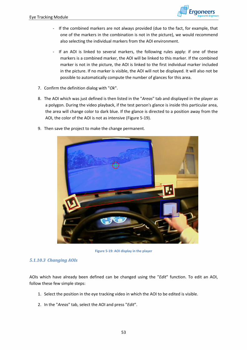
Eye Tracking Module
53
- If the combined markers are not always provided (due to the fact, for example, that
one of the markers in the combination is not in the picture), we would recommend
also selecting the individual markers from the AOI environment.
- If an AOI is linked to several markers, the following rules apply: if one of these
markers is a combined marker, the AOI will be linked to this marker. If the combined
marker is not in the picture, the AOI is linked to the first individual marker included
in the picture. If no marker is visible, the AOI will not be displayed. It will also not be
possible to automatically compute the number of glances for this area.
7. Confirm the definition dialog with "Ok".
8. The AOI which was just defined is then listed in the "Areas" tab and displayed in the player as
a polygon. During the video playback, if the test person's glance is inside this particular area,
the area will change color to dark blue. If the glance is directed to a position away from the
AOI, the color of the AOI is not as intensive (Figure 5-19).
9. Then save the project to make the change permanent.
Figure 5-19: AOI display in the player
5.1.10.3 Changing AOIs
AOIs which have already been defined can be changed using the "Edit" function. To edit an AOI,
follow these few simple steps:
1. Select the position in the eye tracking video in which the AOI to be edited is visible.
2. In the "Areas" tab, select the AOI and press "Edit".
Eye Tracking Module
54
3. The AOI definition dialog is opened (Figure 5-18). Here you can enter the name, the type and
the markers to which the AOI is linked, or you can change the shape of the AOI, as described
in the previous section.
4. Confirm the dialog to accept the changes.
5. Then save the project to make the change permanent.
5.1.10.4 Deleting AOIs
1. Select the AOI you wish to delete in the "Areas" tab and press the "Delete" button.
2. The selected AOI is deleted.
3. Save the project to make the change permanent.
5.1.11 Computing the Glances toward the AOIs
Once the AOIs have been defined, you can start computing the number of glances toward the AOIs.
To do so, proceed as follows:
1. Select the "Compute gaze behavior" entry which can be found in the "Project" menu. This will
compute the number of glances aimed at defined AOIs for all of the people participating in
the study.
2. To compute the number of glances for the current scene, press the "Compute gaze behavior"
button in the "Areas" tab or select the item with the same name in the "Scene" menu.
! Please note that computing the number of glances can take a long time depending on the length
of the eye tracking video and the number of defined AOIs. The D-Lab interface is blocked and the
application cannot be used for this time. For this reason, we would recommend that, should you
wish to compute an entire project, this be done overnight.
5.1.11.1 Deleting Blinks
When a person blinks, the eye is closed for several milliseconds meaning that the pupil cannot be
detected for this duration. If the blink occurs during a glance at a particular object, this can lead to
the glance being split up. To stop this occurring, blinks can be deleted.
The maximum duration of a blink can be set in the "Configuration" dialog in the "Extras" menu
(Figure 5-20). The standard value is 120 ms. This means that gaps which occur between glances and
which are smaller than or equal to the configured value are filled, thus joining together the previous
and subsequent glances.
To delete blinks:
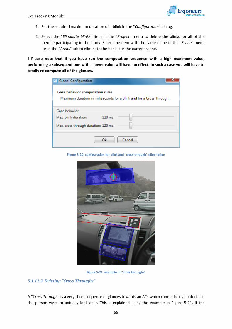
Eye Tracking Module
55
1. Set the required maximum duration of a blink in the "Configuration" dialog.
2. Select the "Eliminate blinks" item in the "Project" menu to delete the blinks for all of the
people participating in the study. Select the item with the same name in the "Scene" menu
or in the "Areas" tab to eliminate the blinks for the current scene.
! Please note that if you have run the computation sequence with a high maximum value,
performing a subsequent one with a lower value will have no effect. In such a case you will have to
totally re-compute all of the glances.
Figure 5-20: configuration for blink and "cross through" elimination
Figure 5-21: example of "cross throughs"
5.1.11.2 Deleting "Cross Throughs"
A "Cross Through" is a very short sequence of glances towards an AOI which cannot be evaluated as if
the person were to actually look at it. This is explained using the example in Figure 5-21. If the
Eye Tracking Module
56
person's focus moves from the rearview mirror to the surface underneath the display, it will briefly
pass or "cross through" the display AOI. This does not mean that the person actually looked at the
display AOI.
"Cross throughs" can be eliminated. The result is that glances toward an AOI which are less than or
equal to the configured maximum value for a cross through (Figure 5-20) are deleted. The settings
can be made in the "Configuration" dialog. The default value for a cross through is 120 ms.
To delete cross throughs:
1. Set the required maximum duration of a cross through in the "Configuration" dialog.
2. Select the "Eliminate cross throughs" item in the "Project" menu to delete the unwanted
glances for all of the people participating in the study. Select the item with the same name in
the "Scene" menu or in the "Areas" tab to eliminate the cross throughs for the current
scene.
! Please note that if you have run the computation sequence with a high maximum value,
performing a subsequent one with a lower value will have no effect. In such a case you will have to
totally re-compute all of the glances.
5.1.12 Visualizing the Glance Behavior
The result of the glance behavior computation is displayed in Figure 5-22. All of the glances towards
each defined AOI are displayed as time bars in the "AOI gaze behavior visualisation" tab. Also, in the
bottom section of the "Areas" tab, the glances towards the AOIs selected under "Project AOIs" and
"Experiment AOIs" are listed. You can organize this list based on the starting time or the duration of
the glance. If you select an entry from this list, the corresponding time interval is highlighted in a
different color and the player jumps to the start of the glance in question (Figure 5-22).
In the bottom section of the "AOI gaze behavior visualisation" tab, a projection of the marked use
case intervals is displayed. You can use this to simultaneously observe the glance behavior and check
if a use case is currently active or not. You can also zoom in to the glances. This makes sense for long
eye tracking videos as you can use it to improve the resolution of the displayed glance behavior. To
zoom in to the glances, use the "Zoom Out", "Zoom In" and "Reset" buttons.
5.1.12.1 Validity Index for Markers and Pupil Detection
To determine the quality of the eye tracking data as regards marker detection and pupil recognition,
the computation of the glances is accompanied by a computation of the so-called validity index. This
index indicates in which video sections the glances cannot be automatically computed as either no
markers ("Marker Index") or no pupil ("Eye Index") have been detected in the video image.
The index is displayed in the bottom section of the "AOI gaze behavior visualisation" tab, in the same
bar with the task intervals. You can choose which of these indices you wish to display by ticking the
"Eye Index" or "Marker Index" box. The results are displayed using colored time bars, as shown in
Figure 5-22.
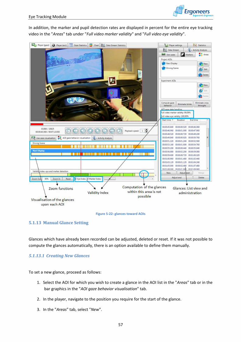
Eye Tracking Module
57
In addition, the marker and pupil detection rates are displayed in percent for the entire eye tracking
video in the "Areas" tab under "Full video marker validity" and "Full video eye validity".
Figure 5-22: glances toward AOIs
5.1.13 Manual Glance Setting
Glances which have already been recorded can be adjusted, deleted or reset. If it was not possible to
compute the glances automatically, there is an option available to define them manually.
5.1.13.1 Creating New Glances
To set a new glance, proceed as follows:
1. Select the AOI for which you wish to create a glance in the AOI list in the "Areas" tab or in the
bar graphics in the "AOI gaze behavior visualisation" tab.
2. In the player, navigate to the position you require for the start of the glance.
3. In the "Areas" tab, select "New".
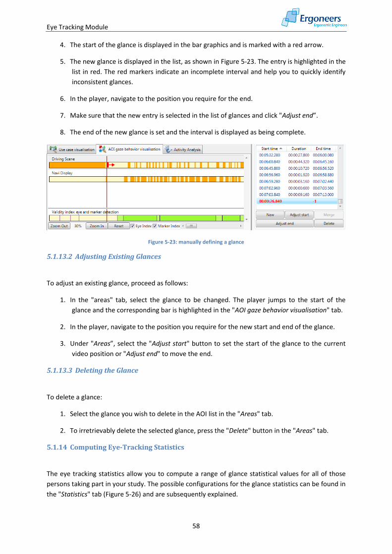
Eye Tracking Module
58
4. The start of the glance is displayed in the bar graphics and is marked with a red arrow.
5. The new glance is displayed in the list, as shown in Figure 5-23. The entry is highlighted in the
list in red. The red markers indicate an incomplete interval and help you to quickly identify
inconsistent glances.
6. In the player, navigate to the position you require for the end.
7. Make sure that the new entry is selected in the list of glances and click "Adjust end”.
8. The end of the new glance is set and the interval is displayed as being complete.
Figure 5-23: manually defining a glance
5.1.13.2 Adjusting Existing Glances
To adjust an existing glance, proceed as follows:
1. In the "areas" tab, select the glance to be changed. The player jumps to the start of the
glance and the corresponding bar is highlighted in the "AOI gaze behavior visualisation" tab.
2. In the player, navigate to the position you require for the new start and end of the glance.
3. Under "Areas”, select the "Adjust start" button to set the start of the glance to the current
video position or "Adjust end" to move the end.
5.1.13.3 Deleting the Glance
To delete a glance:
1. Select the glance you wish to delete in the AOI list in the "Areas" tab.
2. To irretrievably delete the selected glance, press the "Delete" button in the "Areas" tab.
5.1.14 Computing Eye-Tracking Statistics
The eye tracking statistics allow you to compute a range of glance statistical values for all of those
persons taking part in your study. The possible configurations for the glance statistics can be found in
the "Statistics" tab (Figure 5-26) and are subsequently explained.
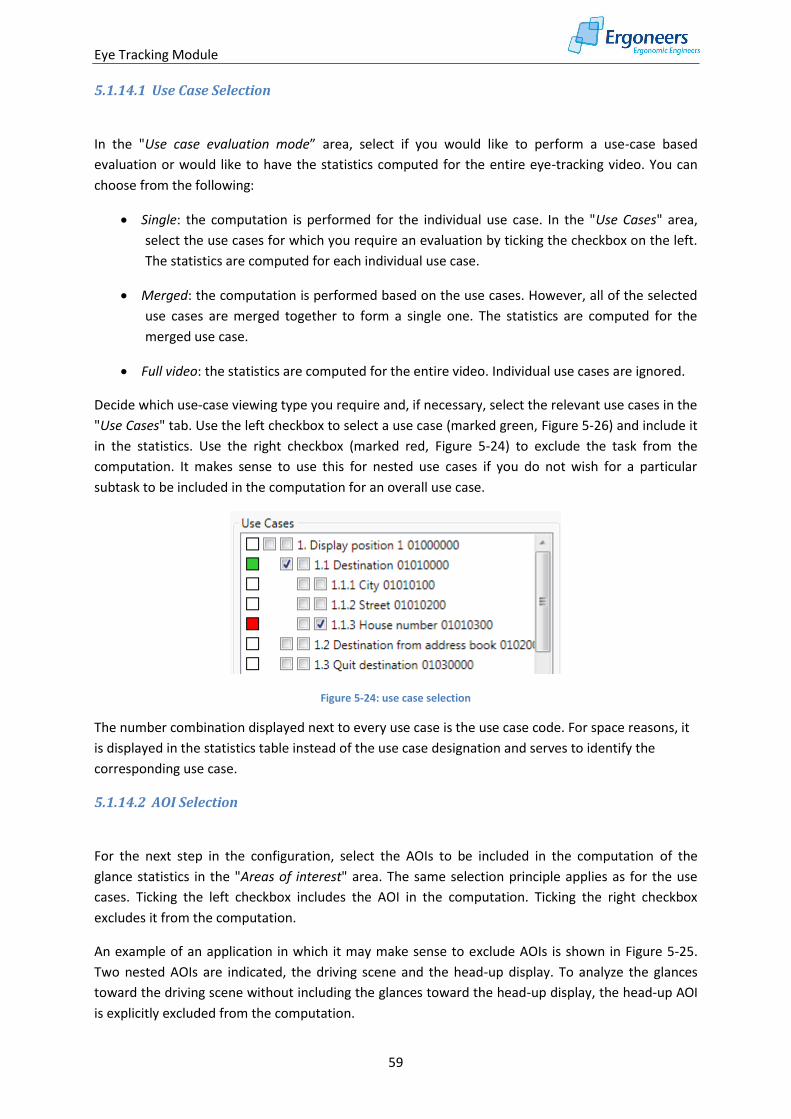
Eye Tracking Module
59
5.1.14.1 Use Case Selection
In the "Use case evaluation mode” area, select if you would like to perform a use-case based
evaluation or would like to have the statistics computed for the entire eye-tracking video. You can
choose from the following:
Single: the computation is performed for the individual use case. In the "Use Cases" area,
select the use cases for which you require an evaluation by ticking the checkbox on the left.
The statistics are computed for each individual use case.
Merged: the computation is performed based on the use cases. However, all of the selected
use cases are merged together to form a single one. The statistics are computed for the
merged use case.
Full video: the statistics are computed for the entire video. Individual use cases are ignored.
Decide which use-case viewing type you require and, if necessary, select the relevant use cases in the
"Use Cases" tab. Use the left checkbox to select a use case (marked green, Figure 5-26) and include it
in the statistics. Use the right checkbox (marked red, Figure 5-24) to exclude the task from the
computation. It makes sense to use this for nested use cases if you do not wish for a particular
subtask to be included in the computation for an overall use case.
Figure 5-24: use case selection
The number combination displayed next to every use case is the use case code. For space reasons, it
is displayed in the statistics table instead of the use case designation and serves to identify the
corresponding use case.
5.1.14.2 AOI Selection
For the next step in the configuration, select the AOIs to be included in the computation of the
glance statistics in the "Areas of interest" area. The same selection principle applies as for the use
cases. Ticking the left checkbox includes the AOI in the computation. Ticking the right checkbox
excludes it from the computation.
An example of an application in which it may make sense to exclude AOIs is shown in Figure 5-25.
Two nested AOIs are indicated, the driving scene and the head-up display. To analyze the glances
toward the driving scene without including the glances toward the head-up display, the head-up AOI
is explicitly excluded from the computation.
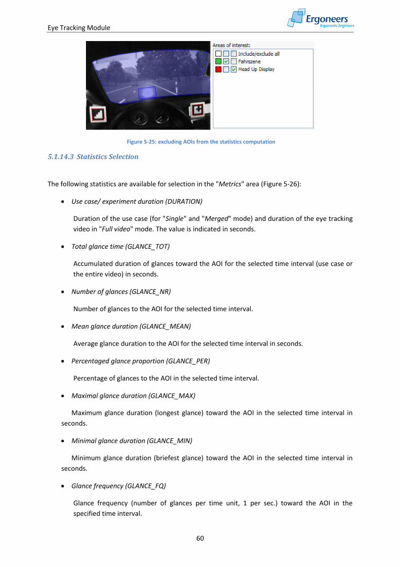
Eye Tracking Module
60
Figure 5-25: excluding AOIs from the statistics computation
5.1.14.3 Statistics Selection
The following statistics are available for selection in the "Metrics" area (Figure 5-26):
Use case/ experiment duration (DURATION)
Duration of the use case (for "Single" and "Merged" mode) and duration of the eye tracking
video in "Full video" mode. The value is indicated in seconds.
Total glance time (GLANCE_TOT)
Accumulated duration of glances toward the AOI for the selected time interval (use case or
the entire video) in seconds.
Number of glances (GLANCE_NR)
Number of glances to the AOI for the selected time interval.
Mean glance duration (GLANCE_MEAN)
Average glance duration to the AOI for the selected time interval in seconds.
Percentaged glance proportion (GLANCE_PER)
Percentage of glances to the AOI in the selected time interval.
Maximal glance duration (GLANCE_MAX)
Maximum glance duration (longest glance) toward the AOI in the selected time interval in
seconds.
Minimal glance duration (GLANCE_MIN)
Minimum glance duration (briefest glance) toward the AOI in the selected time interval in
seconds.
Glance frequency (GLANCE_FQ)
Glance frequency (number of glances per time unit, 1 per sec.) toward the AOI in the
specified time interval.
Eye Tracking Module
61
Horizontal gaze activity (STDDEVX_PUPIL)
Standard deviation of the pupil in the X-axis in pixels. This is a measurement for the search
activity of the glance.
The designation in capital letters which is displayed next to each statistical value is its code. This
value is also displayed in the statistics table and identifies the statistical value.
5.1.14.4 Visualizing Eye-Tracking Statistics
Once you have configured the eye tracking statistics, start the computation process by clicking on the
"Compute metrics" button. Once the computation has been successful, the table with the results is
displayed in the "Table" tab (see Figure 5-27). It is structured as follows:
For each combination of a selected task, AOI and statistic, there is a column which includes
the value of the computed statistic for the corresponding task and AOI.
The test persons are entered in the table's horizontal rows.
The last six rows contain inference statistics about all of the test persons with the following
statistics: sum, mean value, maximum, minimum, standard deviation and variance.
The table's header provides the meaning of the individual columns. The header is made up of the
following:
<Use case code>_<Statistic code>_<AOI name>
Use case code: can be found in the "Statistics" tab next to the use case designation and
identifies the use case.
Statistic code: can be found in the "Statistics" tab next to the use statistical value designation
and identifies the statistical value.
AOI name: the name of the analyzed AOIs, as defined by the user.
5.1.14.5 Exporting the Eye-Tracking Statistics
The eye tracking statistics can be exported in text format and so that they can then be further
examined using other applications such as Excel or SPSS. To do so, press the "Export" button above
the table (Figure 5-27). In the dialog which is then opened, enter the name of the text file and
confirm the dialog with "Save”.
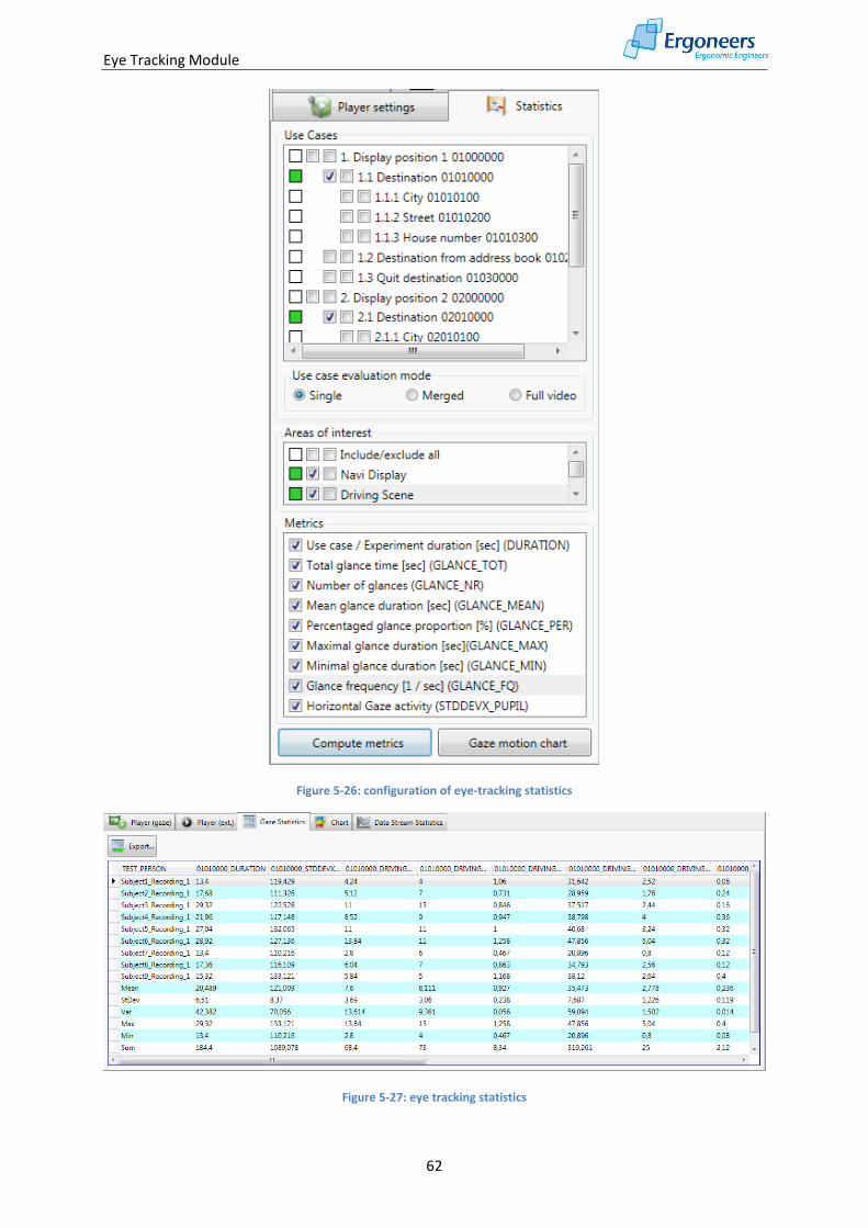
Eye Tracking Module
62
Figure 5-26: configuration of eye-tracking statistics
Figure 5-27: eye tracking statistics
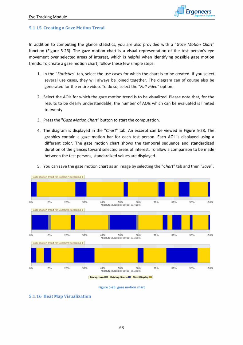
Eye Tracking Module
63
5.1.15 Creating a Gaze Motion Trend
In addition to computing the glance statistics, you are also provided with a "Gaze Motion Chart"
function (Figure 5-26). The gaze motion chart is a visual representation of the test person's eye
movement over selected areas of interest, which is helpful when identifying possible gaze motion
trends. To create a gaze motion chart, follow these few simple steps:
1. In the "Statistics" tab, select the use cases for which the chart is to be created. If you select
several use cases, they will always be joined together. The diagram can of course also be
generated for the entire video. To do so, select the "Full video" option.
2. Select the AOIs for which the gaze motion trend is to be visualized. Please note that, for the
results to be clearly understandable, the number of AOIs which can be evaluated is limited
to twenty.
3. Press the "Gaze Motion Chart" button to start the computation.
4. The diagram is displayed in the "Chart" tab. An excerpt can be viewed in Figure 5-28. The
graphics contain a gaze motion bar for each test person. Each AOI is displayed using a
different color. The gaze motion chart shows the temporal sequence and standardized
duration of the glances toward selected areas of interest. To allow a comparison to be made
between the test persons, standardized values are displayed.
5. You can save the gaze motion chart as an image by selecting the "Chart" tab and then "Save”.
Figure 5-28: gaze motion chart
5.1.16 Heat Map Visualization
Eye Tracking Module
64
The heat map is an option for graphically visualizing the gaze motion. The glances are accumulated
over a specific time and displayed in the player as a colored cloud of dots. The heat maps color
spectrum ranges from blue to red. Short glances are shown in blue. The longer the glance remains in
the area, the more the heat map color changes - to green, yellow and then red.
The heat map is configured in the "Player Settings" setting (Figure 5-29, on the left). The possible
settings are based on the general heat map options (group "General") and how far back the heat map
information is to be stored (group "History").
The "General" options comprise the following:
"Linkage": type of marker linkage. Can be dynamic or static. In the same way as for the AOIs,
the heat map is linked to a selectable marker ("Dynamic”). This allows the gaze motion to be
played back at the right time. Please note that the heat map can only be displayed if the
selected marker is in the picture.
"Static" does not require any link to a marker but will only work if the test person does not
move his or her head or if the eye tracking video has a constant frame (e.g. if a monitor
display is being recorded).
"Spot size": size of a heat map spot.
"Type": “Single" or "Multiple". The "Single" heat map shows the gaze motion for one test
person. "Multiple" combines the gaze motion for several people and is displayed as a heat
map.
To set how far back the data is to be saved ("History" area) for the heat map, the following options
are available:
"Manual": the time interval for which the heat map is to be displayed can be manually
adjusted and can be specified in hours, minutes and seconds. A setting of, for example, 3s
means that, at each point in time, the gaze motion which took place in the last 3 seconds is
displayed as a heat map (Figure 5-29).
"Scene": the gaze motion for the entire eye tracking video is displayed as a heat map.
"Use Case”: the heat map is displayed for a selectable use case.
To configure the heat map, please perform the following steps:
1. In the project overview, select the scene in which the heat map is to be displayed.
2. In the "Player settings" tab, in the "Display" area, select "Heat Map" to activate the heat map
(Figure 5-29).
3. Select the "Linkage" type "Dynamic" and, from the marker list, select the marker to which
the heat map is to be linked.
4. Under "Spot size" set the spot to the required size.
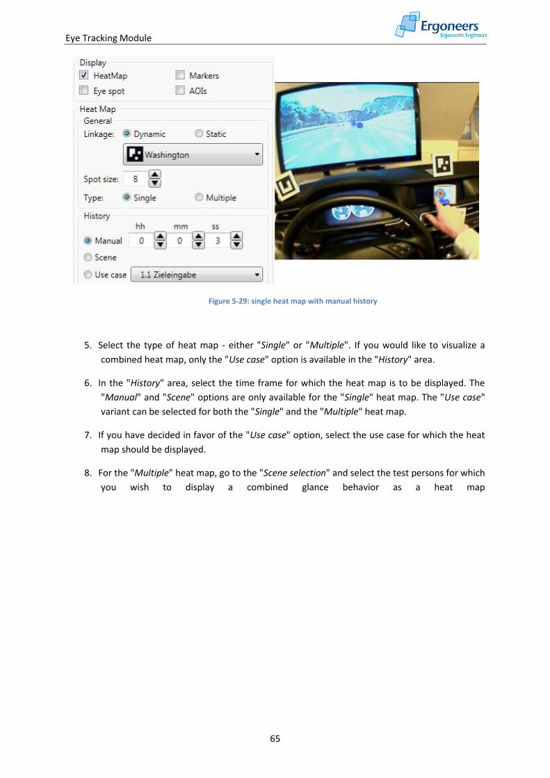
Eye Tracking Module
65
Figure 5-29: single heat map with manual history
5. Select the type of heat map - either "Single" or "Multiple". If you would like to visualize a
combined heat map, only the "Use case" option is available in the "History" area.
6. In the "History" area, select the time frame for which the heat map is to be displayed. The
"Manual" and "Scene" options are only available for the "Single" heat map. The "Use case"
variant can be selected for both the "Single" and the "Multiple" heat map.
7. If you have decided in favor of the "Use case" option, select the use case for which the heat
map should be displayed.
8. For the "Multiple" heat map, go to the "Scene selection" and select the test persons for which
you wish to display a combined glance behavior as a heat map
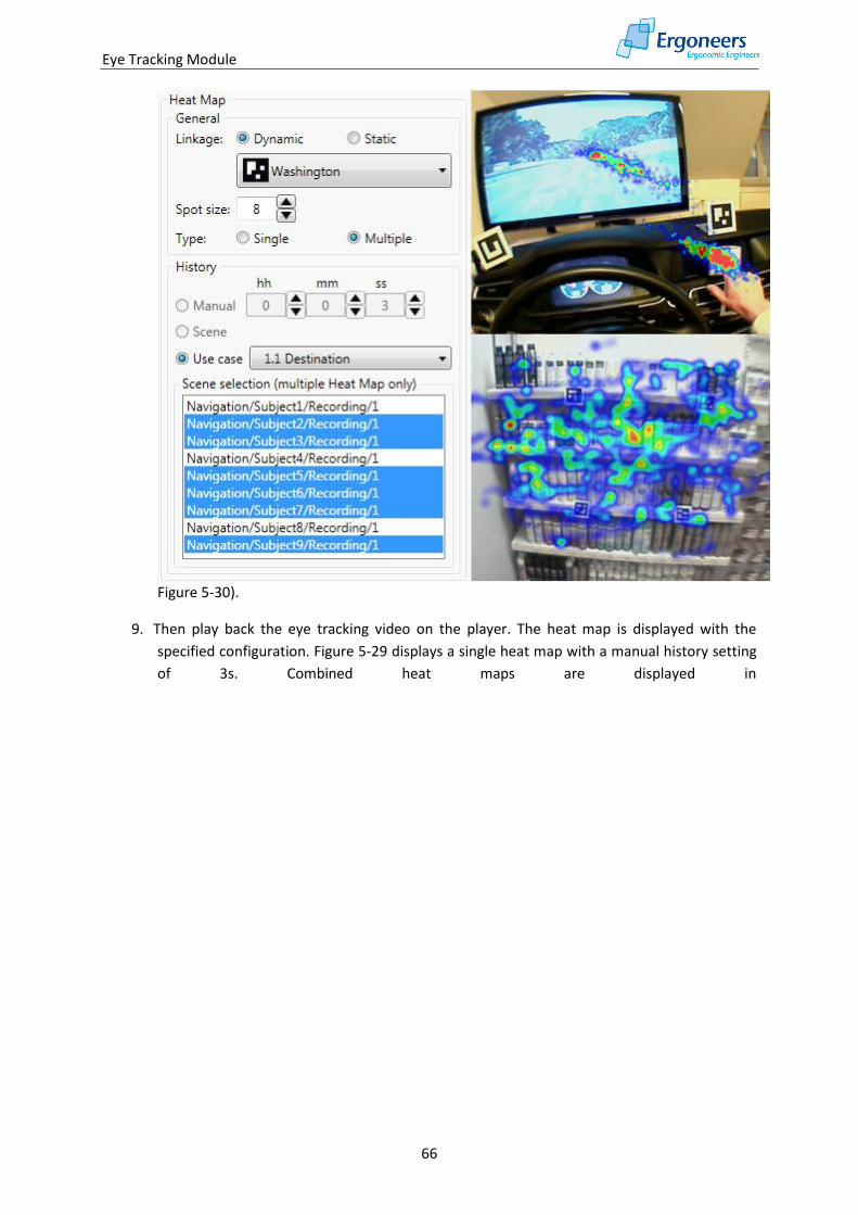
Eye Tracking Module
66
Figure 5-30).
9. Then play back the eye tracking video on the player. The heat map is displayed with the
specified configuration. Figure 5-29 displays a single heat map with a manual history setting
of 3s. Combined heat maps are displayed in
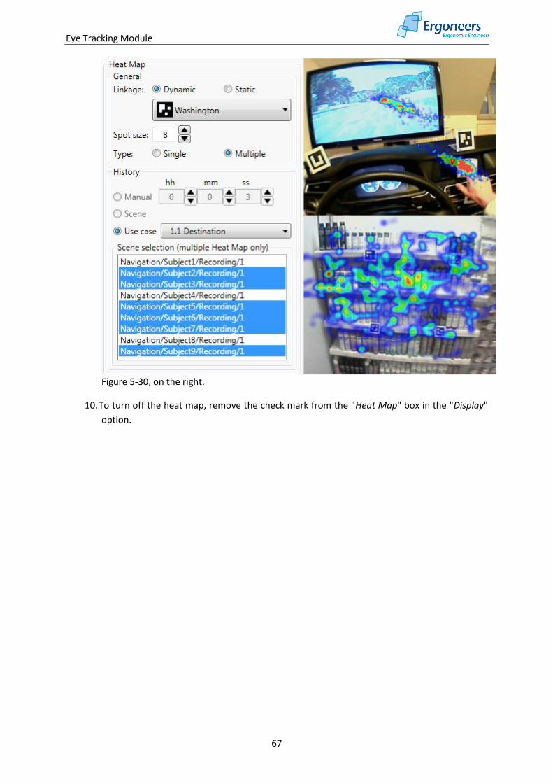
Eye Tracking Module
67
Figure 5-30, on the right.
10. To turn off the heat map, remove the check mark from the "Heat Map" box in the "Display"
option.
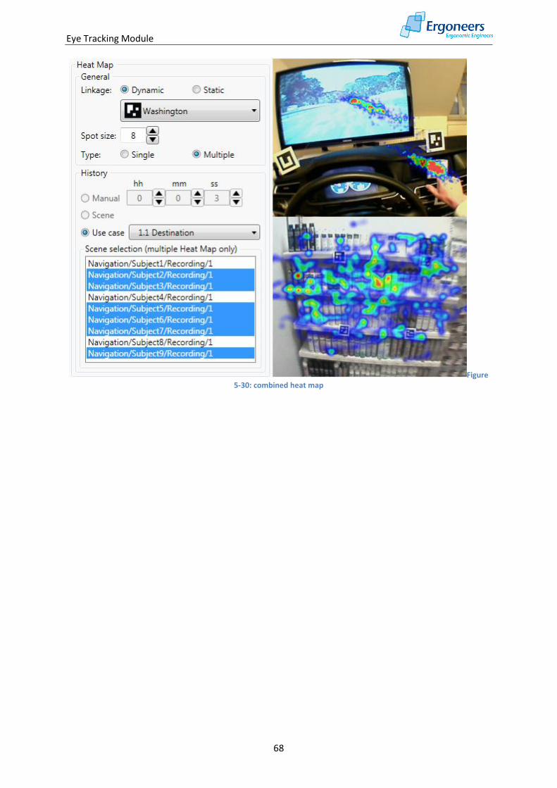
Eye Tracking Module
68
Figure 5-30: combined heat map
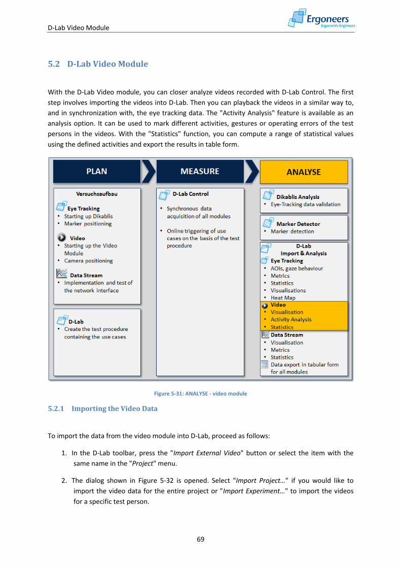
D-Lab Video Module
69
5.2 D-Lab Video Module
With the D-Lab Video module, you can closer analyze videos recorded with D-Lab Control. The first
step involves importing the videos into D-Lab. Then you can playback the videos in a similar way to,
and in synchronization with, the eye tracking data. The "Activity Analysis" feature is available as an
analysis option. It can be used to mark different activities, gestures or operating errors of the test
persons in the videos. With the "Statistics" function, you can compute a range of statistical values
using the defined activities and export the results in table form.
Figure 5-31: ANALYSE - video module
5.2.1 Importing the Video Data
To import the data from the video module into D-Lab, proceed as follows:
1. In the D-Lab toolbar, press the "Import External Video" button or select the item with the
same name in the "Project" menu.
2. The dialog shown in Figure 5-32 is opened. Select "Import Project…" if you would like to
import the video data for the entire project or "Import Experiment…" to import the videos
for a specific test person.
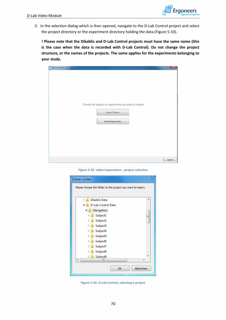
D-Lab Video Module
70
3. In the selection dialog which is then opened, navigate to the D-Lab Control project and select
the project directory or the experiment directory holding the data (Figure 5-33).
! Please note that the Dikablis and D-Lab Control projects must have the same name (this
is the case when the data is recorded with D-Lab Control). Do not change the project
structure, or the names of the projects. The same applies for the experiments belonging to
your study.
Figure 5-32: video importation - project selection
Figure 5-33: D-Lab Control, selecting a project
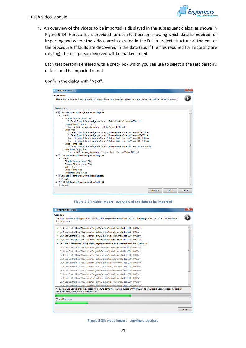
D-Lab Video Module
71
4. An overview of the videos to be imported is displayed in the subsequent dialog, as shown in
Figure 5-34. Here, a list is provided for each test person showing which data is required for
importing and where the videos are integrated in the D-Lab project structure at the end of
the procedure. If faults are discovered in the data (e.g. if the files required for importing are
missing), the test person involved will be marked in red.
Each test person is entered with a check box which you can use to select if the test person's
data should be imported or not.
Confirm the dialog with "Next".
Figure 5-34: video import - overview of the data to be imported
Figure 5-35: video import - copying procedure
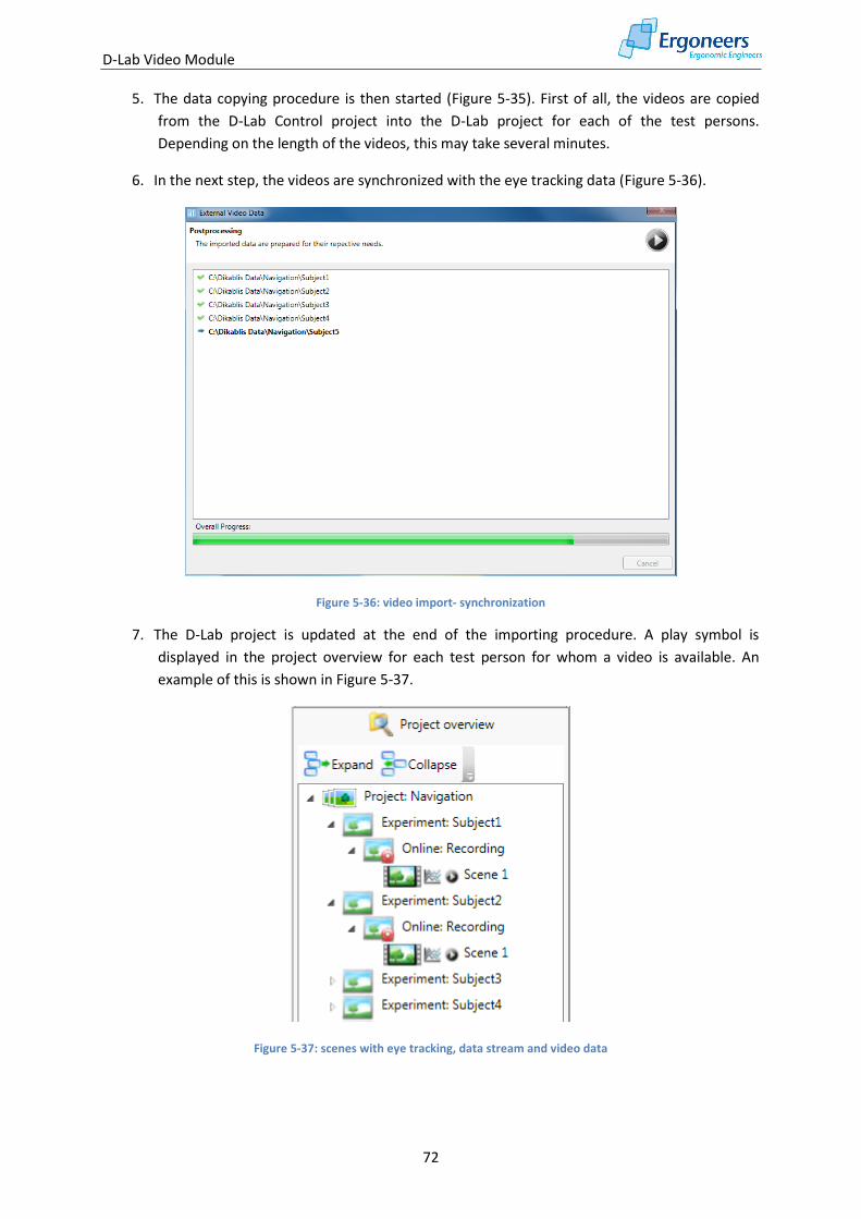
D-Lab Video Module
72
5. The data copying procedure is then started (Figure 5-35). First of all, the videos are copied
from the D-Lab Control project into the D-Lab project for each of the test persons.
Depending on the length of the videos, this may take several minutes.
6. In the next step, the videos are synchronized with the eye tracking data (Figure 5-36).
Figure 5-36: video import- synchronization
7. The D-Lab project is updated at the end of the importing procedure. A play symbol is
displayed in the project overview for each test person for whom a video is available. An
example of this is shown in Figure 5-37.
Figure 5-37: scenes with eye tracking, data stream and video data
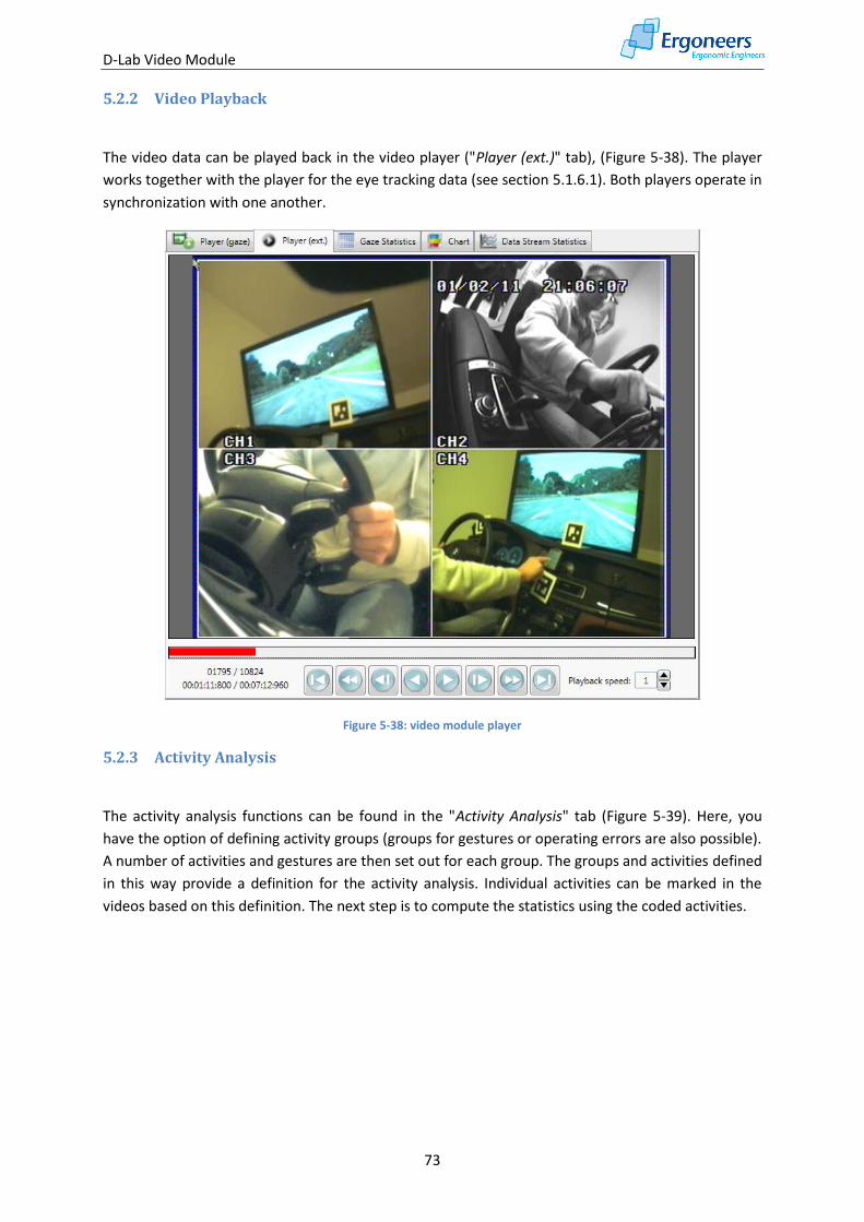
D-Lab Video Module
73
5.2.2 Video Playback
The video data can be played back in the video player ("Player (ext.)" tab), (Figure 5-38). The player
works together with the player for the eye tracking data (see section 5.1.6.1). Both players operate in
synchronization with one another.
Figure 5-38: video module player
5.2.3 Activity Analysis
The activity analysis functions can be found in the "Activity Analysis" tab (Figure 5-39). Here, you
have the option of defining activity groups (groups for gestures or operating errors are also possible).
A number of activities and gestures are then set out for each group. The groups and activities defined
in this way provide a definition for the activity analysis. Individual activities can be marked in the
videos based on this definition. The next step is to compute the statistics using the coded activities.
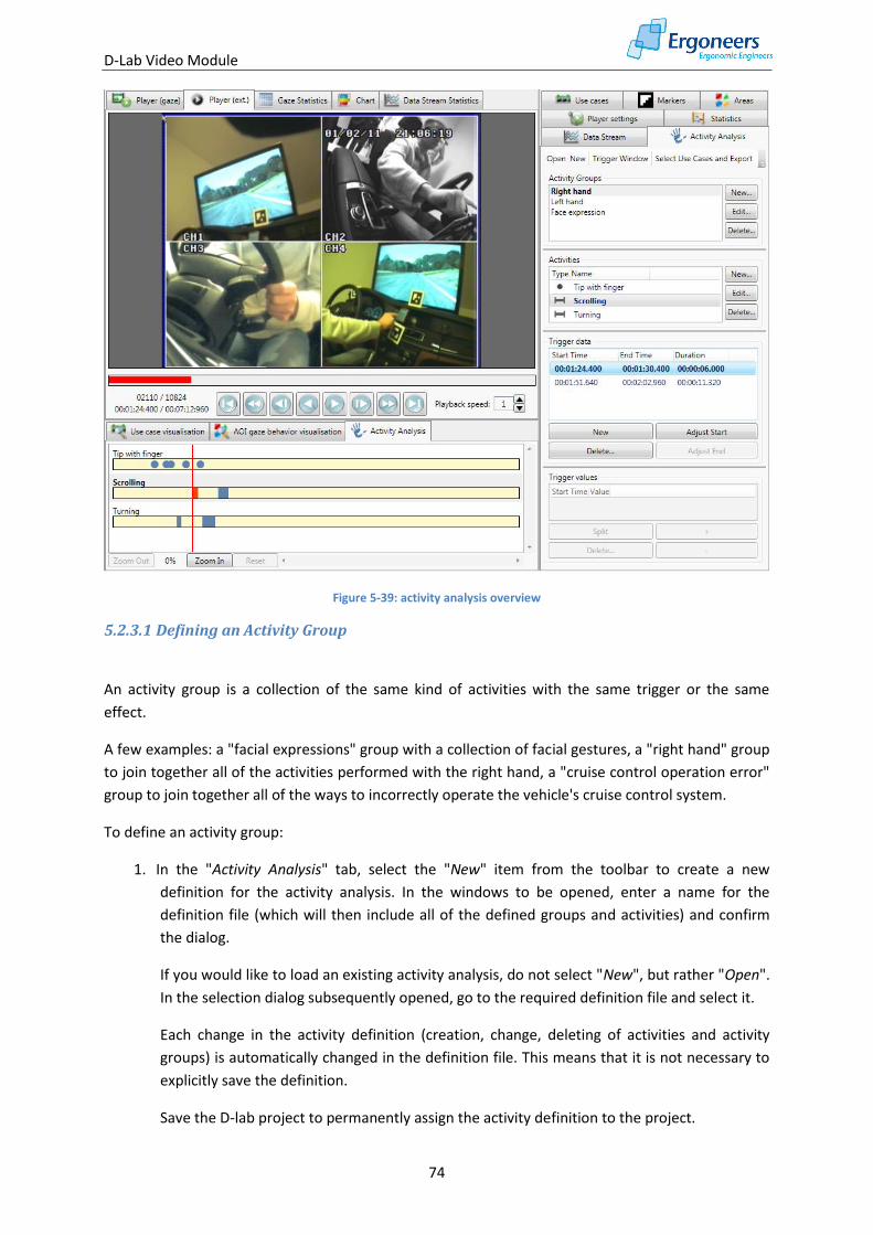
D-Lab Video Module
74
Figure 5-39: activity analysis overview
5.2.3.1 Defining an Activity Group
An activity group is a collection of the same kind of activities with the same trigger or the same
effect.
A few examples: a "facial expressions" group with a collection of facial gestures, a "right hand" group
to join together all of the activities performed with the right hand, a "cruise control operation error"
group to join together all of the ways to incorrectly operate the vehicle's cruise control system.
To define an activity group:
1. In the "Activity Analysis" tab, select the "New" item from the toolbar to create a new
definition for the activity analysis. In the windows to be opened, enter a name for the
definition file (which will then include all of the defined groups and activities) and confirm
the dialog.
If you would like to load an existing activity analysis, do not select "New", but rather "Open".
In the selection dialog subsequently opened, go to the required definition file and select it.
Each change in the activity definition (creation, change, deleting of activities and activity
groups) is automatically changed in the definition file. This means that it is not necessary to
explicitly save the definition.
Save the D-lab project to permanently assign the activity definition to the project.
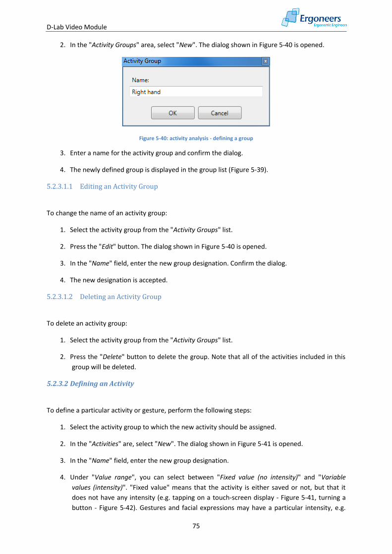
D-Lab Video Module
75
2. In the "Activity Groups" area, select "New". The dialog shown in Figure 5-40 is opened.
Figure 5-40: activity analysis - defining a group
3. Enter a name for the activity group and confirm the dialog.
4. The newly defined group is displayed in the group list (Figure 5-39).
5.2.3.1.1 Editing an Activity Group
To change the name of an activity group:
1. Select the activity group from the "Activity Groups" list.
2. Press the "Edit" button. The dialog shown in Figure 5-40 is opened.
3. In the "Name" field, enter the new group designation. Confirm the dialog.
4. The new designation is accepted.
5.2.3.1.2 Deleting an Activity Group
To delete an activity group:
1. Select the activity group from the "Activity Groups" list.
2. Press the "Delete" button to delete the group. Note that all of the activities included in this
group will be deleted.
5.2.3.2 Defining an Activity
To define a particular activity or gesture, perform the following steps:
1. Select the activity group to which the new activity should be assigned.
2. In the "Activities" are, select "New". The dialog shown in Figure 5-41 is opened.
3. In the "Name" field, enter the new group designation.
4. Under "Value range", you can select between "Fixed value (no intensity)" and "Variable
values (intensity)". "Fixed value" means that the activity is either saved or not, but that it
does not have any intensity (e.g. tapping on a touch-screen display - Figure 5-41, turning a
button - Figure 5-42). Gestures and facial expressions may have a particular intensity, e.g.
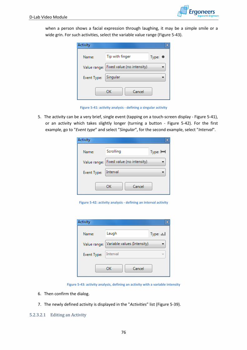
D-Lab Video Module
76
when a person shows a facial expression through laughing, it may be a simple smile or a
wide grin. For such activities, select the variable value range (Figure 5-43).
Figure 5-41: activity analysis - defining a singular activity
5. The activity can be a very brief, single event (tapping on a touch-screen display - Figure 5-41),
or an activity which takes slightly longer (turning a button - Figure 5-42). For the first
example, go to "Event type" and select "Singular", for the second example, select "Interval".
Figure 5-42: activity analysis - defining an interval activity
Figure 5-43: activity analysis, defining an activity with a variable intensity
6. Then confirm the dialog.
7. The newly defined activity is displayed in the "Activities" list (Figure 5-39).
5.2.3.2.1 Editing an Activity
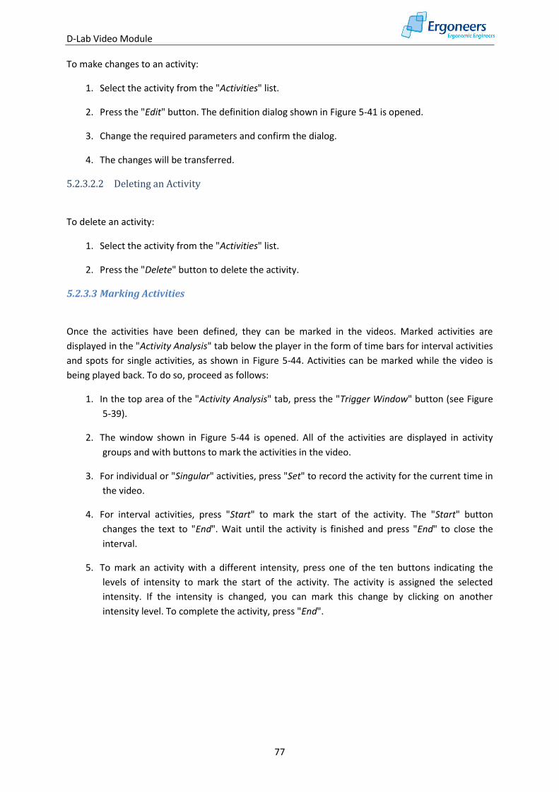
D-Lab Video Module
77
To make changes to an activity:
1. Select the activity from the "Activities" list.
2. Press the "Edit" button. The definition dialog shown in Figure 5-41 is opened.
3. Change the required parameters and confirm the dialog.
4. The changes will be transferred.
5.2.3.2.2 Deleting an Activity
To delete an activity:
1. Select the activity from the "Activities" list.
2. Press the "Delete" button to delete the activity.
5.2.3.3 Marking Activities
Once the activities have been defined, they can be marked in the videos. Marked activities are
displayed in the "Activity Analysis" tab below the player in the form of time bars for interval activities
and spots for single activities, as shown in Figure 5-44. Activities can be marked while the video is
being played back. To do so, proceed as follows:
1. In the top area of the "Activity Analysis" tab, press the "Trigger Window" button (see Figure
5-39).
2. The window shown in Figure 5-44 is opened. All of the activities are displayed in activity
groups and with buttons to mark the activities in the video.
3. For individual or "Singular" activities, press "Set" to record the activity for the current time in
the video.
4. For interval activities, press "Start" to mark the start of the activity. The "Start" button
changes the text to "End". Wait until the activity is finished and press "End" to close the
interval.
5. To mark an activity with a different intensity, press one of the ten buttons indicating the
levels of intensity to mark the start of the activity. The activity is assigned the selected
intensity. If the intensity is changed, you can mark this change by clicking on another
intensity level. To complete the activity, press "End".
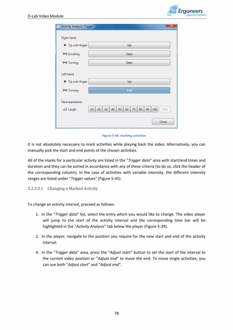
D-Lab Video Module
78
Figure 5-44: marking activities
It is not absolutely necessary to mark activities while playing back the video. Alternatively, you can
manually pick the start and end points of the chosen activities.
All of the marks for a particular activity are listed in the "Trigger data" area with start/end times and
duration and they can be sorted in accordance with any of these criteria (to do so, click the header of
the corresponding column). In the case of activities with variable intensity, the different intensity
ranges are listed under "Trigger values" (Figure 5-45).
5.2.3.3.1 Changing a Marked Activity
To change an activity interval, proceed as follows:
1. In the "Trigger data" list, select the entry which you would like to change. The video player
will jump to the start of the activity interval and the corresponding time bar will be
highlighted in the "Activity Analysis" tab below the player (Figure 5-39).
2. In the player, navigate to the position you require for the new start and end of the activity
interval.
4. In the "Trigger data" area, press the "Adjust start" button to set the start of the interval to
the current video position or "Adjust end" to move the end. To move single activities, you
can use both "Adjust start" and "Adjust end".
D-Lab Video Module
79
Figure 5-45: activity analysis - list of the marked activities
To change the intensity intervals of a marked activity, proceed as follows:
1. In the "Trigger values" area (Figure 5-45 ), select the intensity level to be changed.
2. You can increase or reduce the intensity of the interval with the "+" and "-" buttons.
3. To split an intensity interval, forward or rewind the video player to the position at which the
interval is to be split and then press the "Split" button. The interval is split into two parts.
You can adapt the intensity of the split intervals with the "+" and "-" buttons.
4. To delete an intensity area, select it and press "Delete…".
5.2.3.3.2 Deleting a Marked Activity
To delete an activity interval, proceed as follows:
1. In the "Trigger data" list, select the entry which you would like to delete.
D-Lab Video Module
80
2. In the "Trigger data" area, press the "Delete…" button to delete the marked activity.
5.2.3.4 Computing and Exporting Statistics
The statistics function for the marked activities will compute the following statistical values:
Count
Number of times the activity occurred in the selected time frame (use case or entire video)
Total Duration (not for "singular" activities)
Accumulated duration of the activity for the selected time frame
Mean duration (not for "singular" activities)
Average activity duration for the selected time frame
Mean Intensity (only for activities with variable intensity)
Average intensity of the activities for the selected time frame (weighted according to the
duration of the intensity intervals).
To compute the statistical values, observe the following steps:
1. In the top area of the "Activity Analysis" tab, press the "Select Use Cases and Export" button
(see Figure 5-39).
2. The window shown in Figure 5-46 is opened. Select the use cases for which the statistics are
to be computed. If you are interested in receiving a result for the entire video, insert a check
mark next to "Full Video" in the bottom window section. Then press "OK".
3. In the dialog which is then opened, select the location you wish to save the statistics and
enter a name for the text file you wish to save them in. Confirm the dialog.
4. The statistics for the marked activities are then computed and saved in the specified text file
in table form. Each column contains a statistical value (per use case and per activity). The
test persons are listed in the horizontal rows.
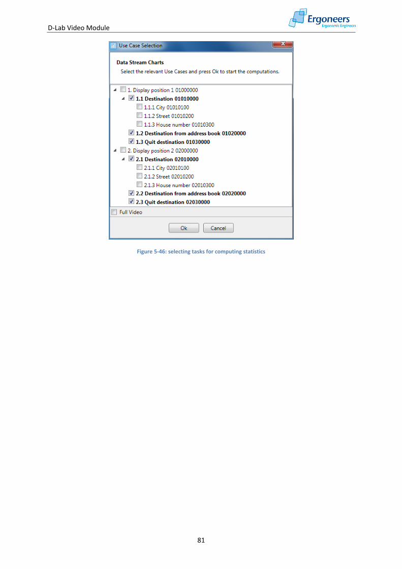
D-Lab Video Module
81
Figure 5-46: selecting tasks for computing statistics
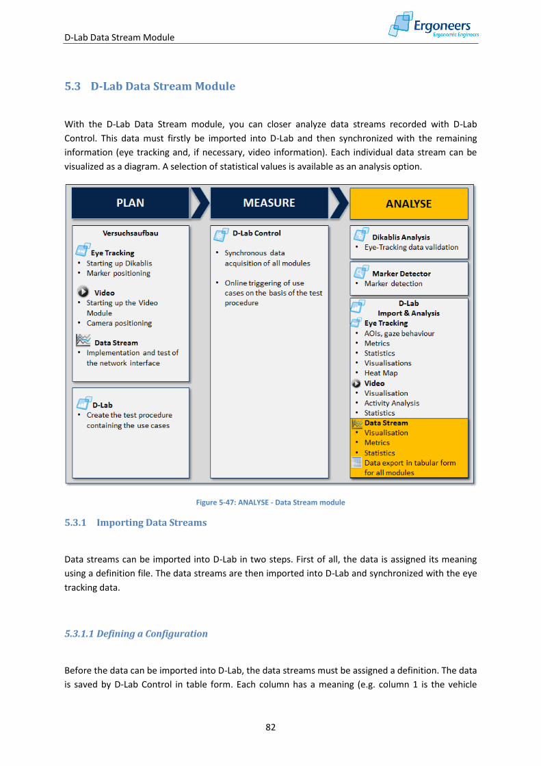
D-Lab Data Stream Module
82
5.3 D-Lab Data Stream Module
With the D-Lab Data Stream module, you can closer analyze data streams recorded with D-Lab
Control. This data must firstly be imported into D-Lab and then synchronized with the remaining
information (eye tracking and, if necessary, video information). Each individual data stream can be
visualized as a diagram. A selection of statistical values is available as an analysis option.
Figure 5-47: ANALYSE - Data Stream module
5.3.1 Importing Data Streams
Data streams can be imported into D-Lab in two steps. First of all, the data is assigned its meaning
using a definition file. The data streams are then imported into D-Lab and synchronized with the eye
tracking data.
5.3.1.1 Defining a Configuration
Before the data can be imported into D-Lab, the data streams must be assigned a definition. The data
is saved by D-Lab Control in table form. Each column has a meaning (e.g. column 1 is the vehicle
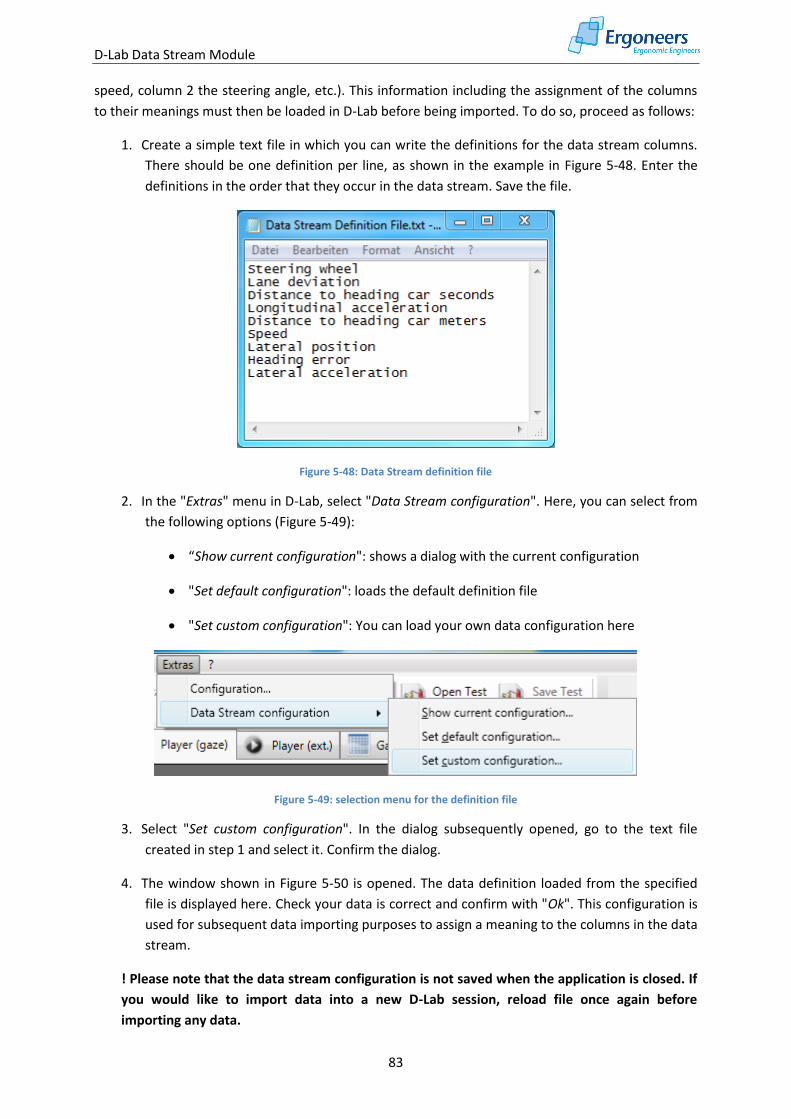
D-Lab Data Stream Module
83
speed, column 2 the steering angle, etc.). This information including the assignment of the columns
to their meanings must then be loaded in D-Lab before being imported. To do so, proceed as follows:
1. Create a simple text file in which you can write the definitions for the data stream columns.
There should be one definition per line, as shown in the example in Figure 5-48. Enter the
definitions in the order that they occur in the data stream. Save the file.
Figure 5-48: Data Stream definition file
2. In the "Extras" menu in D-Lab, select "Data Stream configuration". Here, you can select from
the following options (Figure 5-49):
“Show current configuration": shows a dialog with the current configuration
"Set default configuration": loads the default definition file
"Set custom configuration": You can load your own data configuration here
Figure 5-49: selection menu for the definition file
3. Select "Set custom configuration". In the dialog subsequently opened, go to the text file
created in step 1 and select it. Confirm the dialog.
4. The window shown in Figure 5-50 is opened. The data definition loaded from the specified
file is displayed here. Check your data is correct and confirm with "Ok". This configuration is
used for subsequent data importing purposes to assign a meaning to the columns in the data
stream.
! Please note that the data stream configuration is not saved when the application is closed. If
you would like to import data into a new D-Lab session, reload file once again before
importing any data.
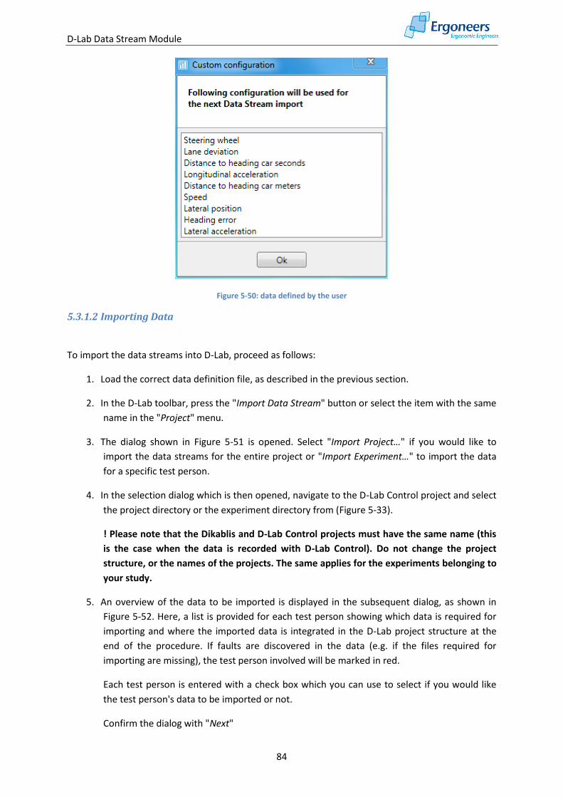
D-Lab Data Stream Module
84
Figure 5-50: data defined by the user
5.3.1.2 Importing Data
To import the data streams into D-Lab, proceed as follows:
1. Load the correct data definition file, as described in the previous section.
2. In the D-Lab toolbar, press the "Import Data Stream" button or select the item with the same
name in the "Project" menu.
3. The dialog shown in Figure 5-51 is opened. Select "Import Project…" if you would like to
import the data streams for the entire project or "Import Experiment…" to import the data
for a specific test person.
4. In the selection dialog which is then opened, navigate to the D-Lab Control project and select
the project directory or the experiment directory from (Figure 5-33).
! Please note that the Dikablis and D-Lab Control projects must have the same name (this
is the case when the data is recorded with D-Lab Control). Do not change the project
structure, or the names of the projects. The same applies for the experiments belonging to
your study.
5. An overview of the data to be imported is displayed in the subsequent dialog, as shown in
Figure 5-52. Here, a list is provided for each test person showing which data is required for
importing and where the imported data is integrated in the D-Lab project structure at the
end of the procedure. If faults are discovered in the data (e.g. if the files required for
importing are missing), the test person involved will be marked in red.
Each test person is entered with a check box which you can use to select if you would like
the test person's data to be imported or not.
Confirm the dialog with "Next"
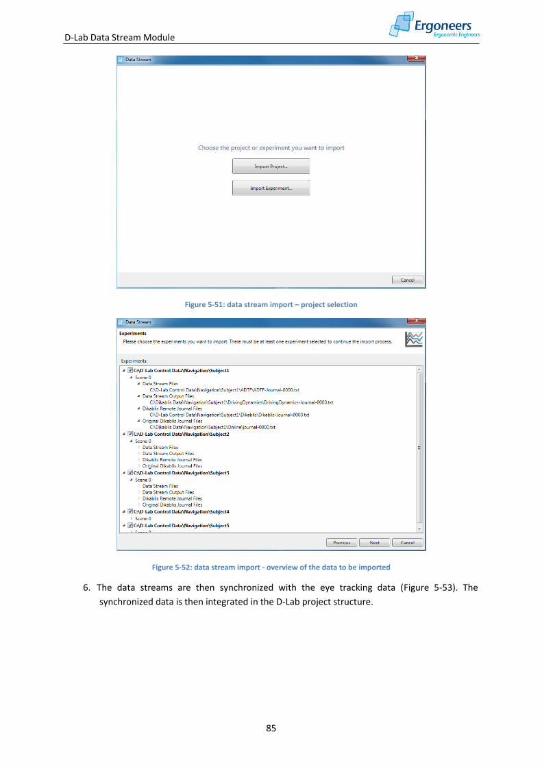
D-Lab Data Stream Module
85
Figure 5-51: data stream import – project selection
Figure 5-52: data stream import - overview of the data to be imported
6. The data streams are then synchronized with the eye tracking data (Figure 5-53). The
synchronized data is then integrated in the D-Lab project structure.
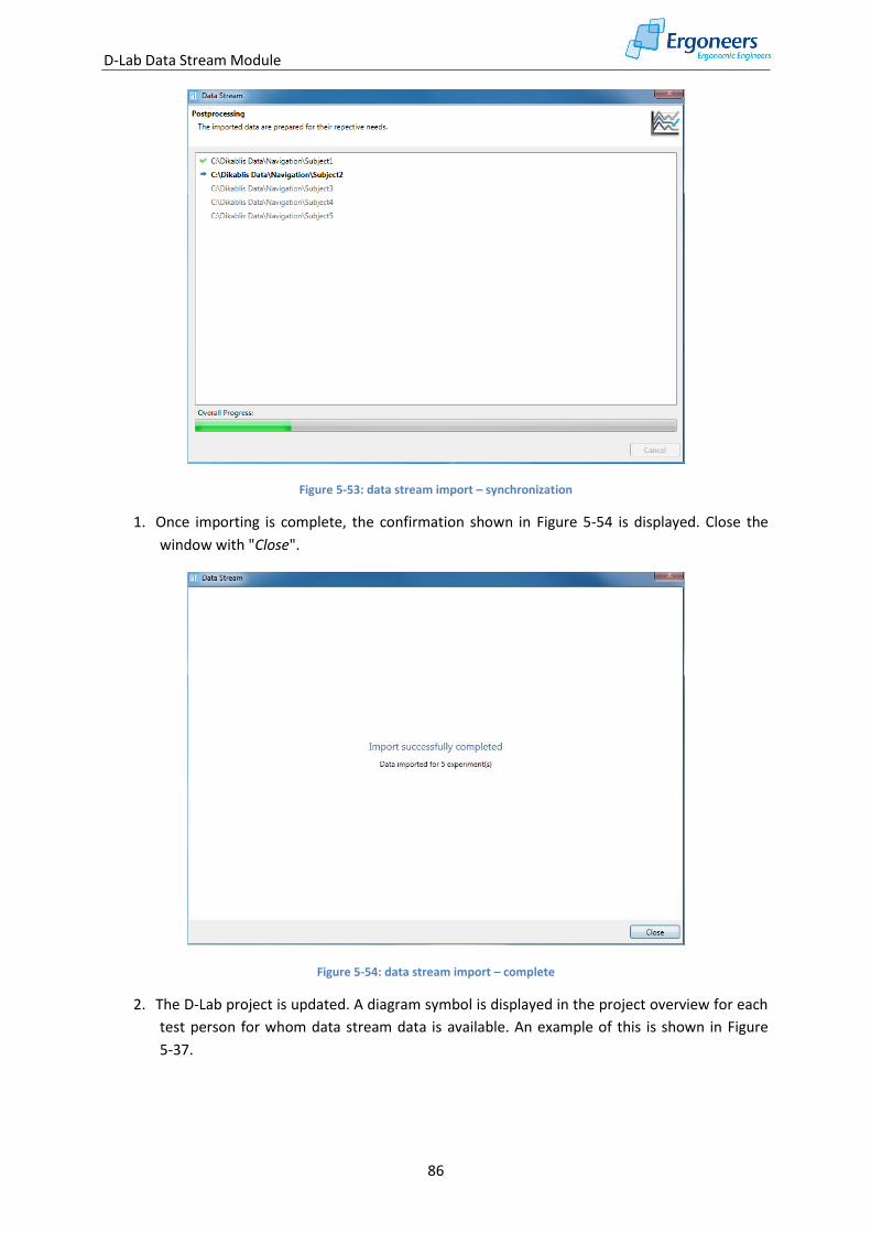
D-Lab Data Stream Module
86
Figure 5-53: data stream import – synchronization
1. Once importing is complete, the confirmation shown in Figure 5-54 is displayed. Close the
window with "Close".
Figure 5-54: data stream import – complete
2. The D-Lab project is updated. A diagram symbol is displayed in the project overview for each
test person for whom data stream data is available. An example of this is shown in Figure
5-37.
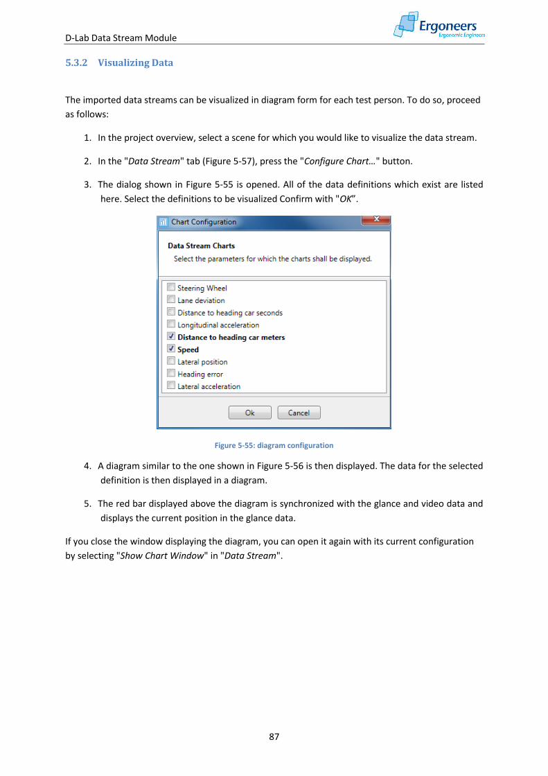
D-Lab Data Stream Module
87
5.3.2 Visualizing Data
The imported data streams can be visualized in diagram form for each test person. To do so, proceed
as follows:
1. In the project overview, select a scene for which you would like to visualize the data stream.
2. In the "Data Stream" tab (Figure 5-57), press the "Configure Chart…" button.
3. The dialog shown in Figure 5-55 is opened. All of the data definitions which exist are listed
here. Select the definitions to be visualized Confirm with "OK”.
Figure 5-55: diagram configuration
4. A diagram similar to the one shown in Figure 5-56 is then displayed. The data for the selected
definition is then displayed in a diagram.
5. The red bar displayed above the diagram is synchronized with the glance and video data and
displays the current position in the glance data.
If you close the window displaying the diagram, you can open it again with its current configuration
by selecting "Show Chart Window" in "Data Stream".
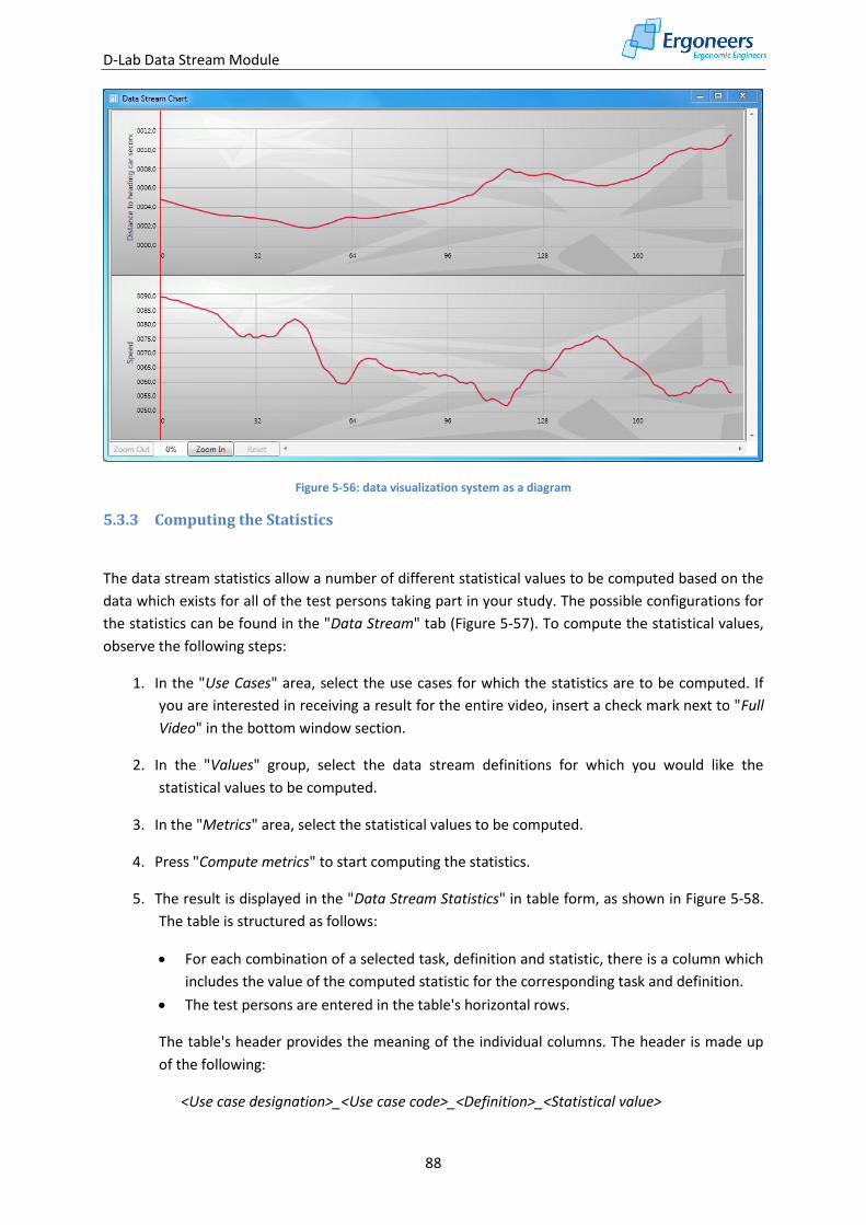
D-Lab Data Stream Module
88
Figure 5-56: data visualization system as a diagram
5.3.3 Computing the Statistics
The data stream statistics allow a number of different statistical values to be computed based on the
data which exists for all of the test persons taking part in your study. The possible configurations for
the statistics can be found in the "Data Stream" tab (Figure 5-57). To compute the statistical values,
observe the following steps:
1. In the "Use Cases" area, select the use cases for which the statistics are to be computed. If
you are interested in receiving a result for the entire video, insert a check mark next to "Full
Video" in the bottom window section.
2. In the "Values" group, select the data stream definitions for which you would like the
statistical values to be computed.
3. In the "Metrics" area, select the statistical values to be computed.
4. Press "Compute metrics" to start computing the statistics.
5. The result is displayed in the "Data Stream Statistics" in table form, as shown in Figure 5-58.
The table is structured as follows:
For each combination of a selected task, definition and statistic, there is a column which
includes the value of the computed statistic for the corresponding task and definition.
The test persons are entered in the table's horizontal rows.
The table's header provides the meaning of the individual columns. The header is made up
of the following:
<Use case designation>_<Use case code>_<Definition>_<Statistical value>
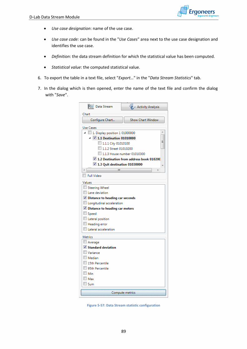
D-Lab Data Stream Module
89
Use case designation: name of the use case.
Use case code: can be found in the "Use Cases" area next to the use case designation and
identifies the use case.
Definition: the data stream definition for which the statistical value has been computed.
Statistical value: the computed statistical value.
6. To export the table in a text file, select "Export…" in the "Data Stream Statistics" tab.
7. In the dialog which is then opened, enter the name of the text file and confirm the dialog
with "Save".
Figure 5-57: Data Stream statistic configuration
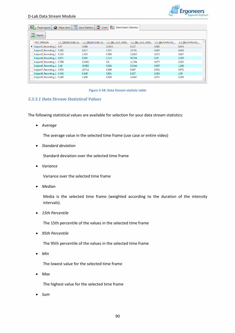
D-Lab Data Stream Module
90
Figure 5-58: Data Stream statistic table
5.3.3.1 Data Stream Statistical Values
The following statistical values are available for selection for your data stream statistics:
Average
The average value in the selected time frame (use case or entire video)
Standard deviation
Standard deviation over the selected time frame
Variance
Variance over the selected time frame
Median
Media is the selected time frame (weighted according to the duration of the intensity
intervals).
15th Percentile
The 15th percentile of the values in the selected time frame
95th Percentile
The 95th percentile of the values in the selected time frame
Min
The lowest value for the selected time frame
Max
The highest value for the selected time frame
Sum
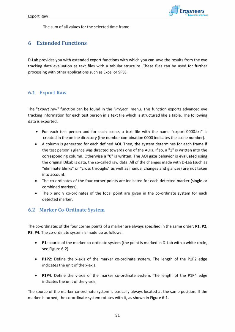
Export Raw
91
The sum of all values for the selected time frame
6 Extended Functions
D-Lab provides you with extended export functions with which you can save the results from the eye
tracking data evaluation as text files with a tabular structure. These files can be used for further
processing with other applications such as Excel or SPSS.
6.1 Export Raw
The "Export raw" function can be found in the "Project" menu. This function exports advanced eye
tracking information for each test person in a text file which is structured like a table. The following
data is exported:
For each test person and for each scene, a text file with the name "export-0000.txt" is
created in the online directory (the number combination 0000 indicates the scene number).
A column is generated for each defined AOI. Then, the system determines for each frame if
the test person's glance was directed towards one of the AOIs. If so, a "1" is written into the
corresponding column. Otherwise a "0" is written. The AOI gaze behavior is evaluated using
the original Dikablis data, the so-called raw data. All of the changes made with D-Lab (such as
"eliminate blinks" or "cross throughs" as well as manual changes and glances) are not taken
into account.
The co-ordinates of the four corner points are indicated for each detected marker (single or
combined markers).
The x and y co-ordinates of the focal point are given in the co-ordinate system for each
detected marker.
6.2 Marker Co-Ordinate System
The co-ordinates of the four corner points of a marker are always specified in the same order: P1, P2,
P3, P4. The co-ordinate system is made up as follows:
P1: source of the marker co-ordinate system (the point is marked in D-Lab with a white circle,
see Figure 6-2).
P1P2: Define the x-axis of the marker co-ordinate system. The length of the P1P2 edge
indicates the unit of the x-axis.
P1P4: Define the y-axis of the marker co-ordinate system. The length of the P1P4 edge
indicates the unit of the y-axis.
The source of the marker co-ordinate system is basically always located at the same position. If the
marker is turned, the co-ordinate system rotates with it, as shown in Figure 6-1.
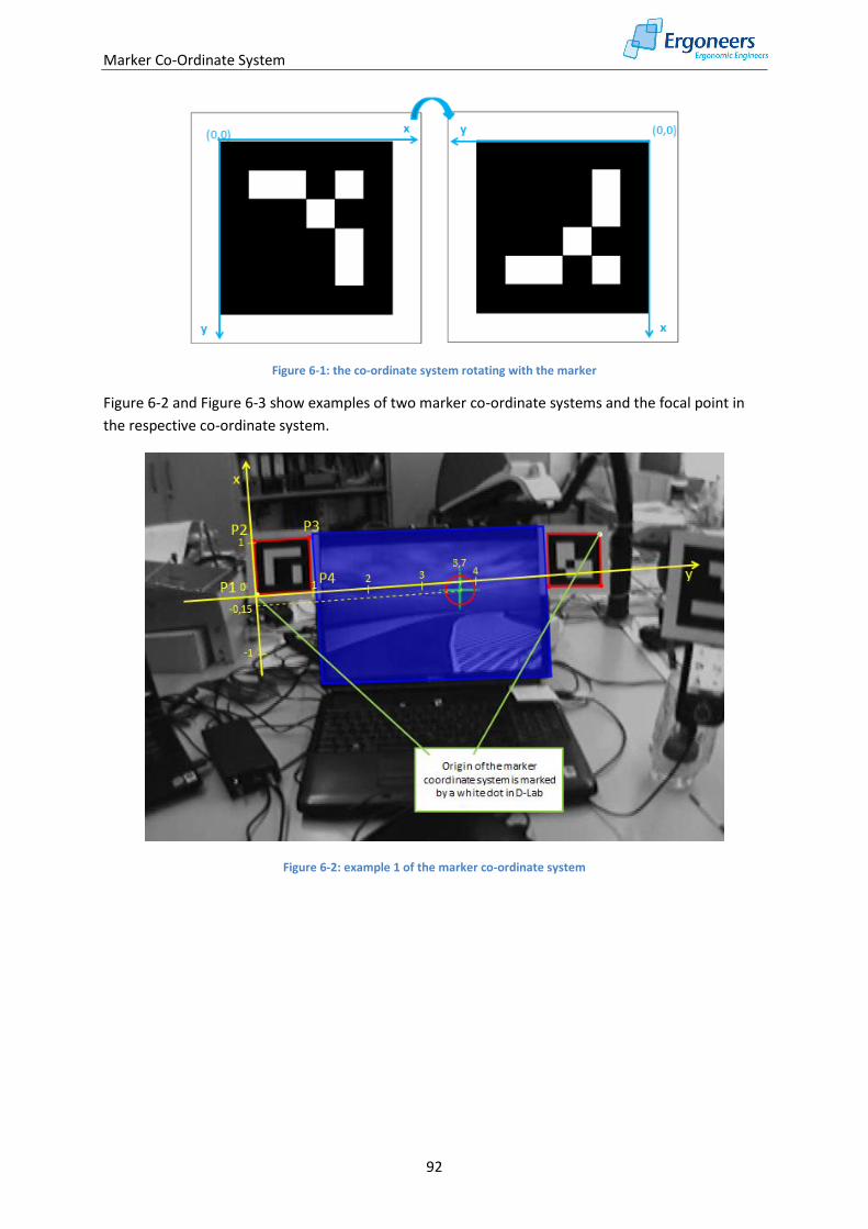
Marker Co-Ordinate System
92
Figure 6-1: the co-ordinate system rotating with the marker
Figure 6-2 and Figure 6-3 show examples of two marker co-ordinate systems and the focal point in
the respective co-ordinate system.
Figure 6-2: example 1 of the marker co-ordinate system
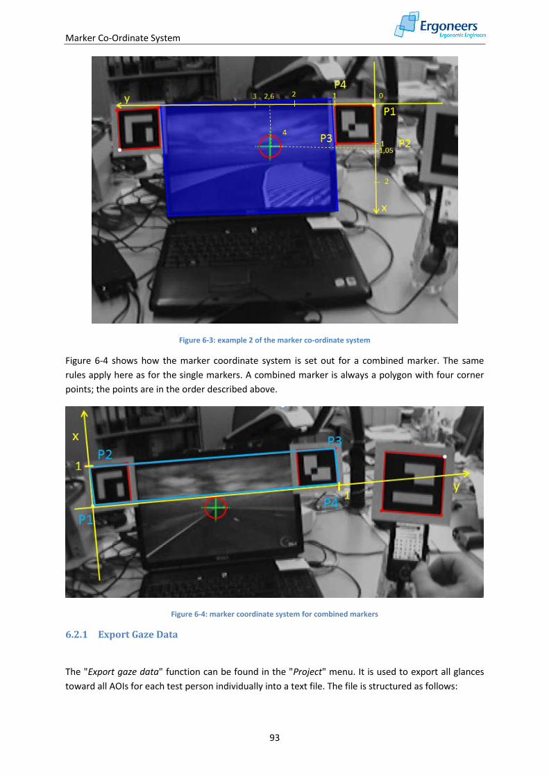
Marker Co-Ordinate System
93
Figure 6-3: example 2 of the marker co-ordinate system
Figure 6-4 shows how the marker coordinate system is set out for a combined marker. The same
rules apply here as for the single markers. A combined marker is always a polygon with four corner
points; the points are in the order described above.
Figure 6-4: marker coordinate system for combined markers
6.2.1 Export Gaze Data
The "Export gaze data" function can be found in the "Project" menu. It is used to export all glances
toward all AOIs for each test person individually into a text file. The file is structured as follows:
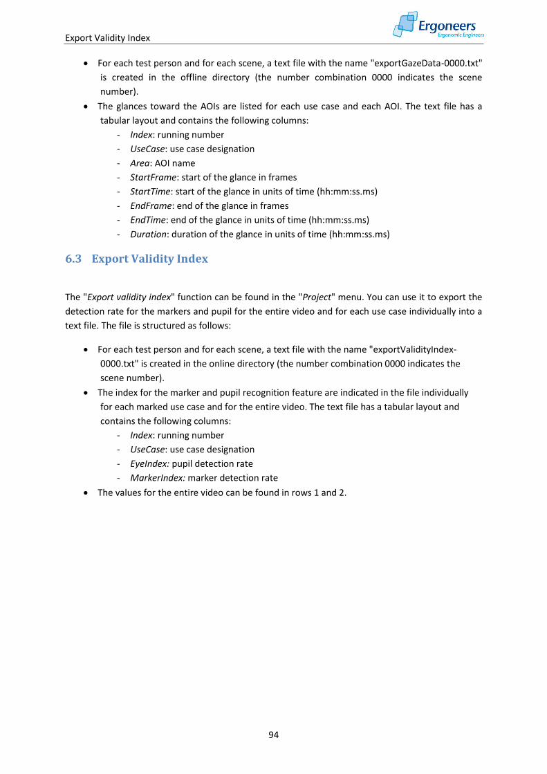
Export Validity Index
94
For each test person and for each scene, a text file with the name "exportGazeData-0000.txt"
is created in the offline directory (the number combination 0000 indicates the scene
number).
The glances toward the AOIs are listed for each use case and each AOI. The text file has a
tabular layout and contains the following columns:
- Index: running number
- UseCase: use case designation
- Area: AOI name
- StartFrame: start of the glance in frames
- StartTime: start of the glance in units of time (hh:mm:ss.ms)
- EndFrame: end of the glance in frames
- EndTime: end of the glance in units of time (hh:mm:ss.ms)
- Duration: duration of the glance in units of time (hh:mm:ss.ms)
6.3 Export Validity Index
The "Export validity index" function can be found in the "Project" menu. You can use it to export the
detection rate for the markers and pupil for the entire video and for each use case individually into a
text file. The file is structured as follows:
For each test person and for each scene, a text file with the name "exportValidityIndex-
0000.txt" is created in the online directory (the number combination 0000 indicates the
scene number).
The index for the marker and pupil recognition feature are indicated in the file individually
for each marked use case and for the entire video. The text file has a tabular layout and
contains the following columns:
- Index: running number
- UseCase: use case designation
- EyeIndex: pupil detection rate
- MarkerIndex: marker detection rate
The values for the entire video can be found in rows 1 and 2.
Glossary
95
Glossary
Area of Interest, AOI
Objects or areas in the test environment for which the glance behavior is to be examined are marked
as areas of interest.
Use Case
Time window which displays a task to be carried out during the test. The use case is recorded by
marking the start and end of the task.
Glance
Time during which the test person's is looking at a defined image area (area of interest).
Experiment, test person, test
Part of a study. Refers to the observation of an individual person as part of the examination. A study
is made up of a number of tests.
License stick
Allows applications to be executed and contains licensing data. The corresponding stick must be
connected to a USB port of a recording computer before the applications (recording software,
analysis software) can be started.
Study, Behavior Study
This means an examination for observing the behavior of a group of persons with regard to a specific
issue.
Test Procedure
Includes all parts of the experiments and all of the use cases to be performed. An instruction on how
the test should be carried out.
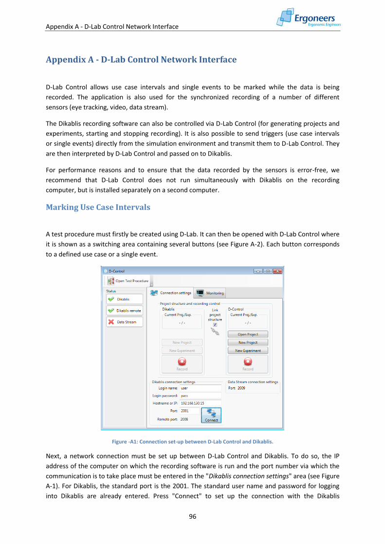
Appendix A - D-Lab Control Network Interface
96
Appendix A - D-Lab Control Network Interface
D-Lab Control allows use case intervals and single events to be marked while the data is being
recorded. The application is also used for the synchronized recording of a number of different
sensors (eye tracking, video, data stream).
The Dikablis recording software can also be controlled via D-Lab Control (for generating projects and
experiments, starting and stopping recording). It is also possible to send triggers (use case intervals
or single events) directly from the simulation environment and transmit them to D-Lab Control. They
are then interpreted by D-Lab Control and passed on to Dikablis.
For performance reasons and to ensure that the data recorded by the sensors is error-free, we
recommend that D-Lab Control does not run simultaneously with Dikablis on the recording
computer, but is installed separately on a second computer.
Marking Use Case Intervals
A test procedure must firstly be created using D-Lab. It can then be opened with D-Lab Control where
it is shown as a switching area containing several buttons (see Figure A-2). Each button corresponds
to a defined use case or a single event.
Figure -A1: Connection set-up between D-Lab Control and Dikablis.
Next, a network connection must be set up between D-Lab Control and Dikablis. To do so, the IP
address of the computer on which the recording software is run and the port number via which the
communication is to take place must be entered in the "Dikablis connection settings" area (see Figure
A-1). For Dikablis, the standard port is the 2001. The standard user name and password for logging
into Dikablis are already entered. Press "Connect" to set up the connection with the Dikablis
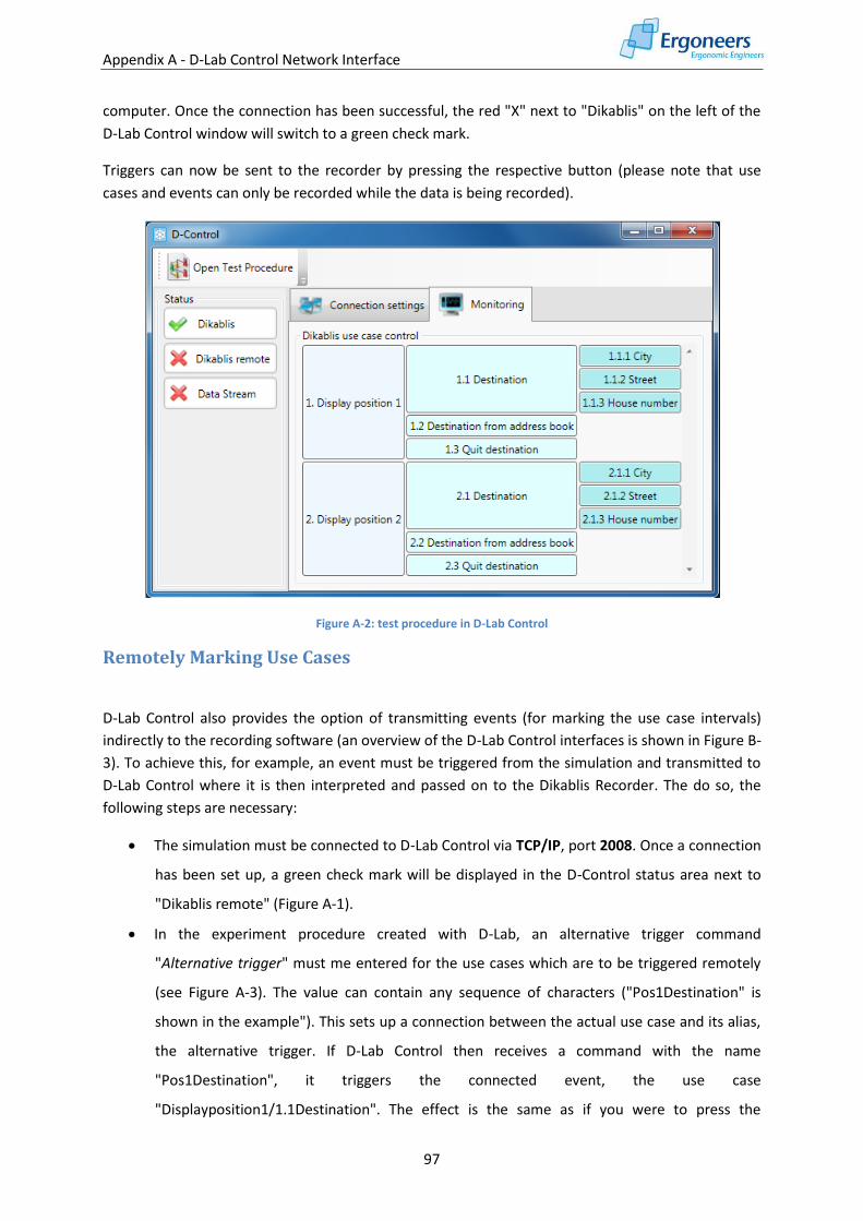
Appendix A - D-Lab Control Network Interface
97
computer. Once the connection has been successful, the red "X" next to "Dikablis" on the left of the
D-Lab Control window will switch to a green check mark.
Triggers can now be sent to the recorder by pressing the respective button (please note that use
cases and events can only be recorded while the data is being recorded).
Figure A-2: test procedure in D-Lab Control
Remotely Marking Use Cases
D-Lab Control also provides the option of transmitting events (for marking the use case intervals)
indirectly to the recording software (an overview of the D-Lab Control interfaces is shown in Figure B-
3). To achieve this, for example, an event must be triggered from the simulation and transmitted to
D-Lab Control where it is then interpreted and passed on to the Dikablis Recorder. The do so, the
following steps are necessary:
The simulation must be connected to D-Lab Control via TCP/IP, port 2008. Once a connection
has been set up, a green check mark will be displayed in the D-Control status area next to
"Dikablis remote" (Figure A-1).
In the experiment procedure created with D-Lab, an alternative trigger command
"Alternative trigger" must me entered for the use cases which are to be triggered remotely
(see Figure A-3). The value can contain any sequence of characters ("Pos1Destination" is
shown in the example"). This sets up a connection between the actual use case and its alias,
the alternative trigger. If D-Lab Control then receives a command with the name
"Pos1Destination", it triggers the connected event, the use case
"Displayposition1/1.1Destination". The effect is the same as if you were to press the
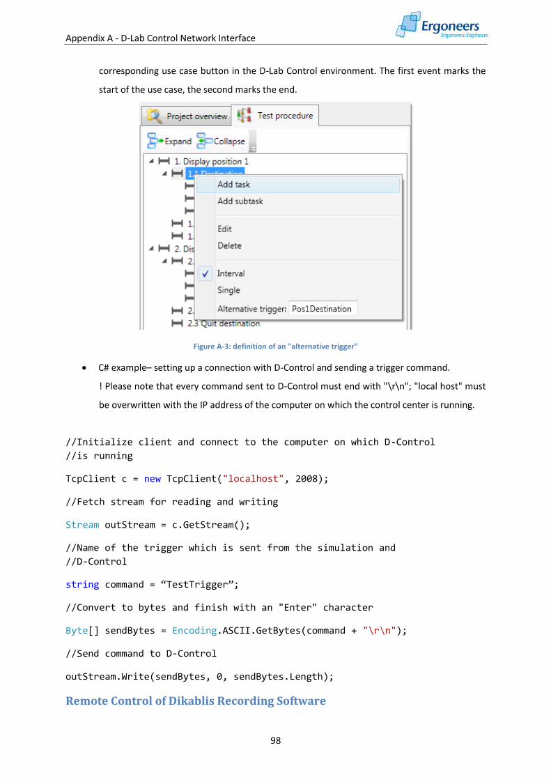
Appendix A - D-Lab Control Network Interface
98
corresponding use case button in the D-Lab Control environment. The first event marks the
start of the use case, the second marks the end.
Figure A-3: definition of an "alternative trigger"
C# example– setting up a connection with D-Control and sending a trigger command.
! Please note that every command sent to D-Control must end with "\r\n"; "local host" must
be overwritten with the IP address of the computer on which the control center is running.
//Initialize client and connect to the computer on which D-Control
//is running
TcpClient c = new TcpClient("localhost", 2008);
//Fetch stream for reading and writing
Stream outStream = c.GetStream();
//Name of the trigger which is sent from the simulation and
//D-Control
string command = “TestTrigger”;
//Convert to bytes and finish with an "Enter" character
Byte[] sendBytes = Encoding.ASCII.GetBytes(command + "\r\n");
//Send command to D-Control
outStream.Write(sendBytes, 0, sendBytes.Length);
Remote Control of Dikablis Recording Software
Appendix A - D-Lab Control Network Interface
99
The following recording software functions can be controlled remotely via D-Lab Control:
Create project:
string command = “project ProjectName”;
Byte[] sendBytes = Encoding.ASCII.GetBytes(command + "\r\n");
When doing so, "ProjectName" is the name of the project and can be a string of characters
(umlauts, spaces and non-standard characters are not permitted).
Creating an experiment:
string command = “experiment ExperimentName”;
Byte[] sendBytes = Encoding.ASCII.GetBytes(command + "\r\n");
When doing so, "ExperimentName" is the name of the experiment and can be a string of
characters (umlauts, spaces and non-standard characters are not permitted).
Starting recording:
string command = “start recording”;
Byte[] sendBytes = Encoding.ASCII.GetBytes(command + "\r\n");
Stopping recording:
string command = “stop recording”;
Byte[] sendBytes = Encoding.ASCII.GetBytes(command + "\r\n");
Please note that an experiment can only be created if a project is open in the recording software and
the recording can only be started once an experiment has been opened.
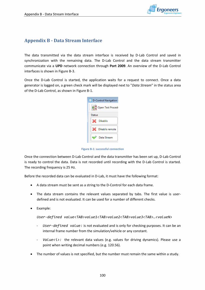
Appendix B - Data Stream Interface
100
Appendix B - Data Stream Interface
The data transmitted via the data stream interface is received by D-Lab Control and saved in
synchronization with the remaining data. The D-Lab Control and the data stream transmitter
communicate via a UPD network connection through Port 2009. An overview of the D-Lab Control
interfaces is shown in Figure B-3.
Once the D-Lab Control is started, the application waits for a request to connect. Once a data
generator is logged on, a green check mark will be displayed next to "Data Stream" in the status area
of the D-Lab Control, as shown in Figure B-1.
Figure B-1: successful connection
Once the connection between D-Lab Control and the data transmitter has been set up, D-Lab Control
is ready to control the data. Data is not recorded until recording with the D-Lab Control is started.
The recording frequency is 25 Hz.
Before the recorded data can be evaluated in D-Lab, it must have the following format:
A data stream must be sent as a string to the D-Control for each data frame.
The data stream contains the relevant values separated by tabs. The first value is user-
defined and is not evaluated. It can be used for a number of different checks.
Example:
User-defined value<TAB>value1<TAB>value2<TAB>value3<TAB>…<valueN>
- User-defined value: is not evaluated and is only for checking purposes. It can be an
internal frame number from the simulation/vehicle or any constant.
- Value<i>: the relevant data values (e.g. values for driving dynamics). Please use a
point when writing decimal numbers (e.g. 120.56).
The number of values is not specified, but the number must remain the same within a study.
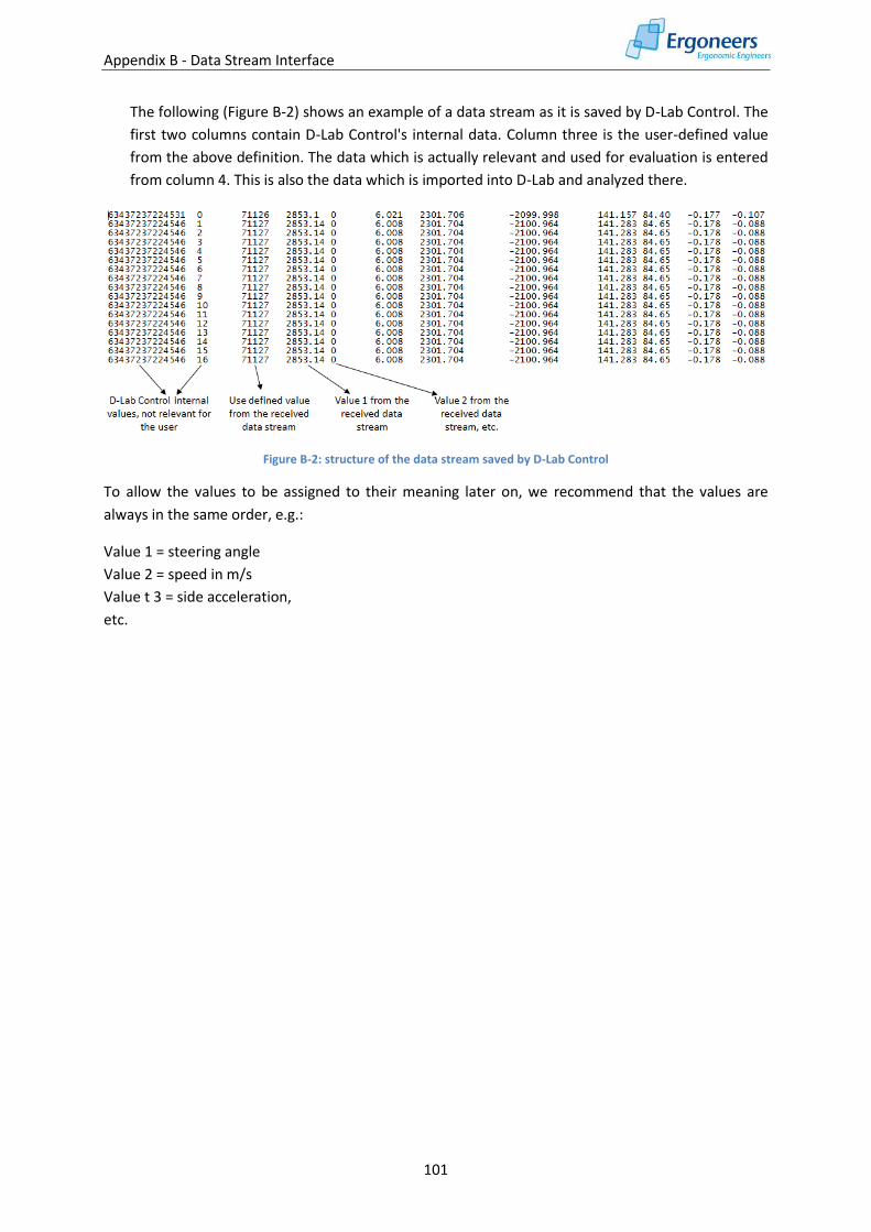
Appendix B - Data Stream Interface
101
The following (Figure B-2) shows an example of a data stream as it is saved by D-Lab Control. The
first two columns contain D-Lab Control's internal data. Column three is the user-defined value
from the above definition. The data which is actually relevant and used for evaluation is entered
from column 4. This is also the data which is imported into D-Lab and analyzed there.
Figure B-2: structure of the data stream saved by D-Lab Control
To allow the values to be assigned to their meaning later on, we recommend that the values are
always in the same order, e.g.:
Value 1 = steering angle
Value 2 = speed in m/s
Value t 3 = side acceleration,
etc.
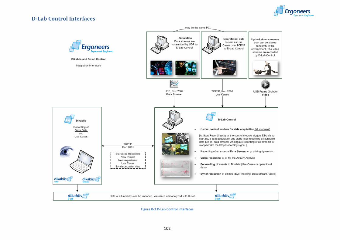
D-Lab Control Interfaces
102
Figure B-3 D-Lab Control interfaces
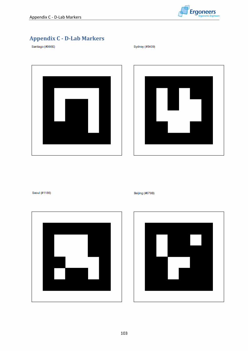
Appendix C - D-Lab Markers
103
Appendix C - D-Lab Markers
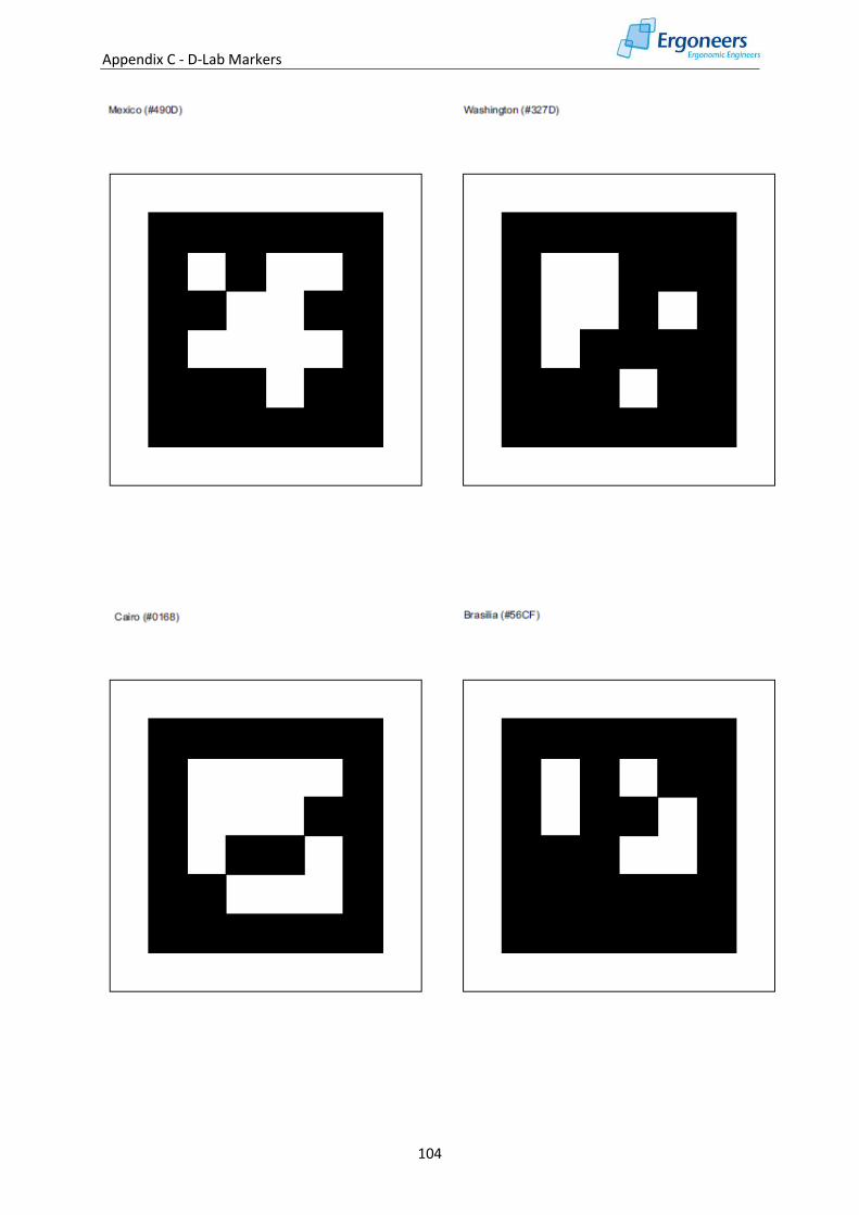
Appendix C - D-Lab Markers
104
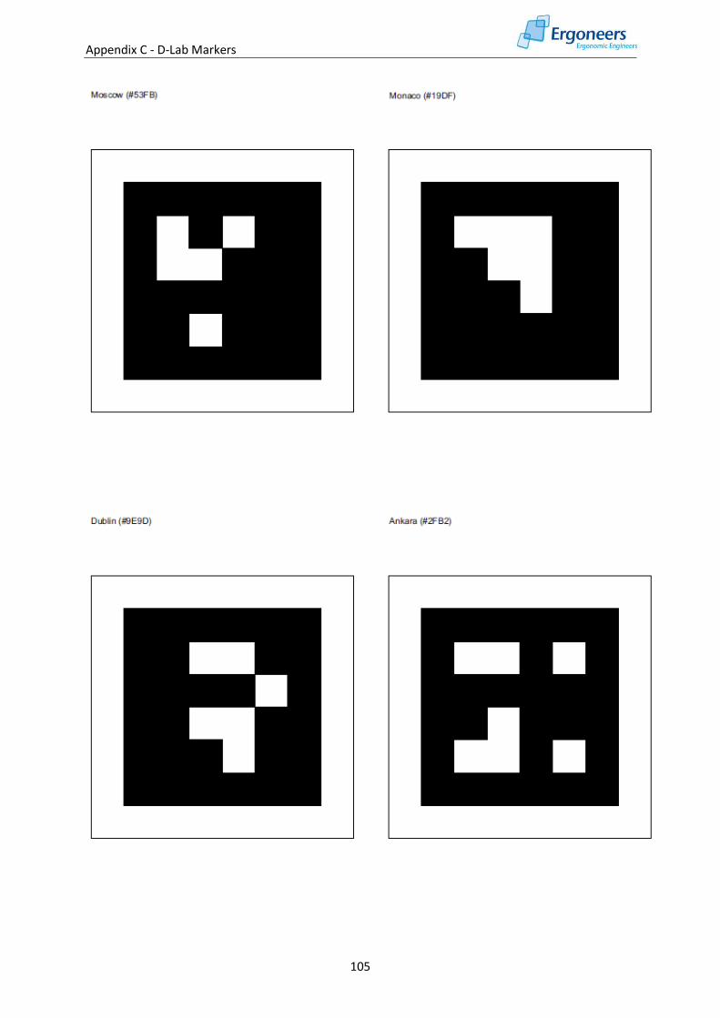
Appendix C - D-Lab Markers
105
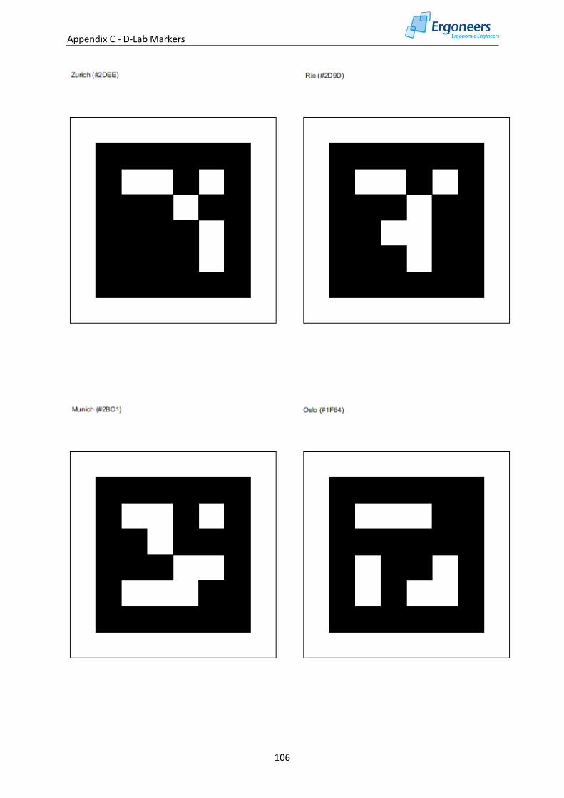
Appendix C - D-Lab Markers
106

![[Réveil en Form’] Analyse des concepts de Fab Lab, … · Centre d’Excellence en Technologies de l’Information et de la Communication [Réveil en Form’] Analyse des concepts](https://img.pdfslide.us/doc/110x75/5b9e56b509d3f2083f8b8363/reveil-en-form-analyse-des-concepts-de-fab-lab-centre-dexcellence.jpg)