D i s cr i m i n a n t a n a l y s i s i n R QM M A

3/5/2018 Discriminant analysis in R (1)

file:///C:/Users/emanuele.taufer/Google%20Drive/2%20CORSI/5%20QMMA%20-%20MIM/0%20Labs/L4-LDA-eng.html#(1) 1/26

Discriminant analysis in R

QMMAEmanuele Taufer



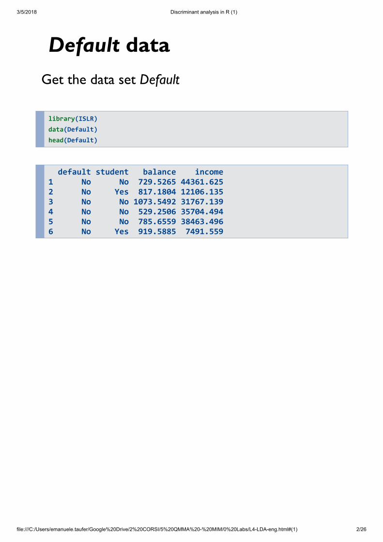
Default dataGet the data set Default

library(ISLR) data(Default) head(Default)

default student balance income 1 No No 729.5265 44361.625 2 No Yes 817.1804 12106.135 3 No No 1073.5492 31767.139 4 No No 529.2506 35704.494 5 No No 785.6559 38463.496 6 No Yes 919.5885 7491.559



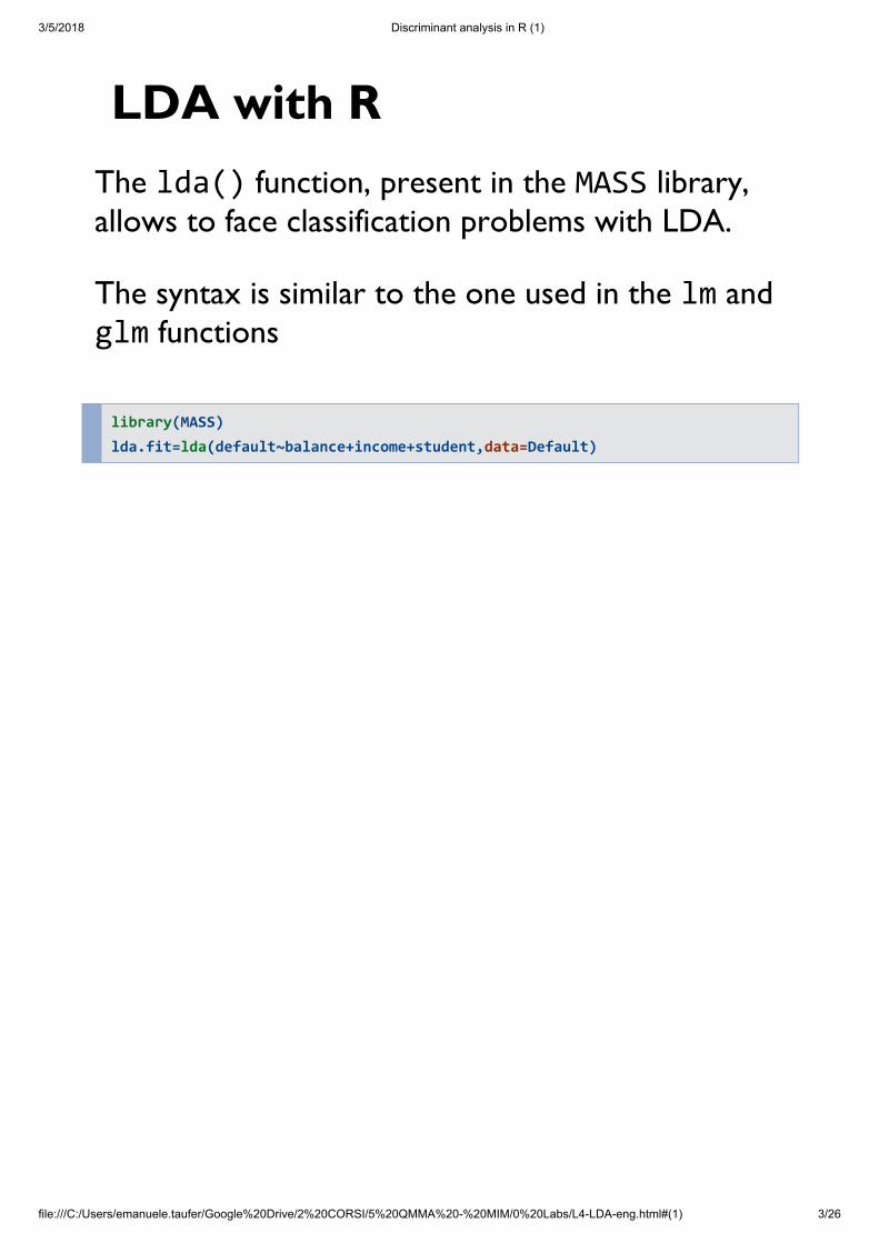
LDA with RThe lda() function, present in the MASS library,allows to face classification problems with LDA.

The syntax is similar to the one used in the lm andglm functions

library(MASS) lda.fit=lda(default~balance+income+student,data=Default)



Output

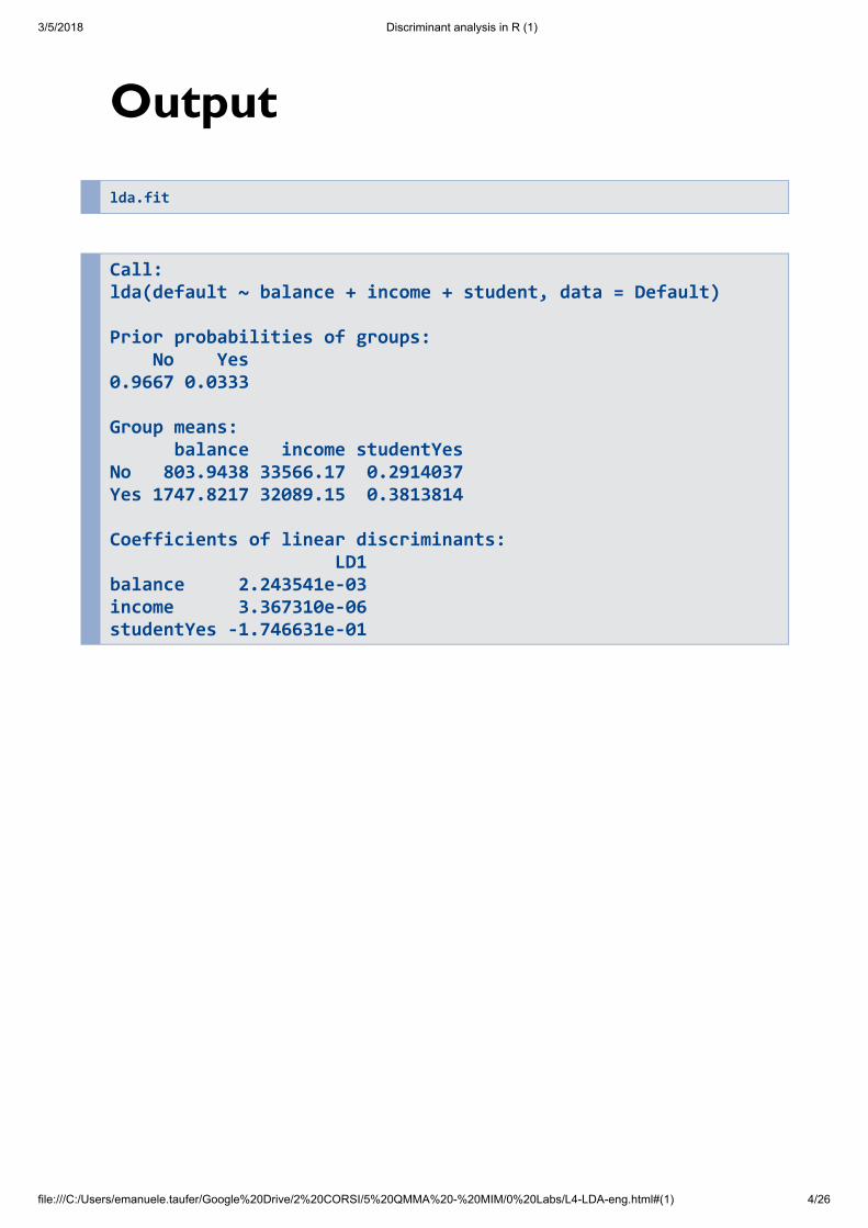
lda.fit

Call: lda(default ~ balance + income + student, data = Default) Prior probabilities of groups: No Yes 0.9667 0.0333 Group means: balance income studentYes No 803.9438 33566.17 0.2914037 Yes 1747.8217 32089.15 0.3813814 Coefficients of linear discriminants: LD1 balance 2.243541e-03 income 3.367310e-06 studentYes -1.746631e-01



Output analysis

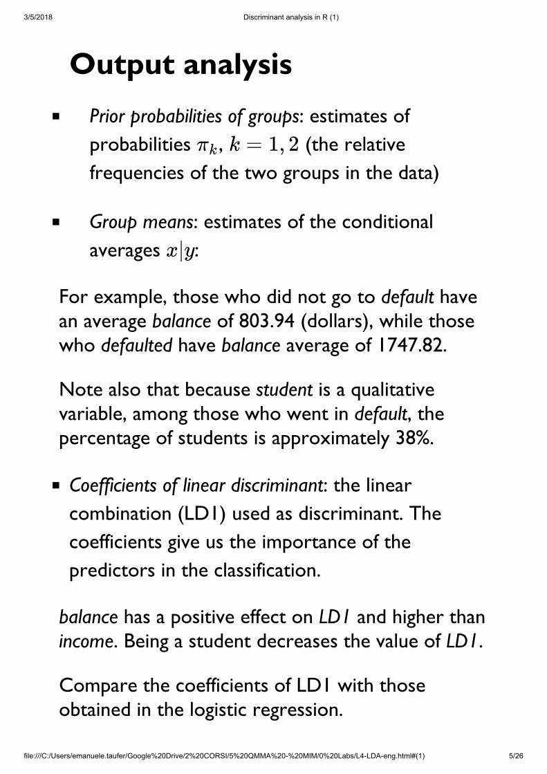
Prior probabilities of groups: estimates ofprobabilities , (the relativefrequencies of the two groups in the data)

Group means: estimates of the conditionalaverages :

For example, those who did not go to default havean average balance of 803.94 (dollars), while thosewho defaulted have balance average of 1747.82.

Note also that because student is a qualitativevariable, among those who went in default, thepercentage of students is approximately 38%.

Coefficients of linear discriminant: the linearcombination (LD1) used as discriminant. Thecoefficients give us the importance of thepredictors in the classification.

balance has a positive effect on LD1 and higher thanincome. Being a student decreases the value of LD1.

Compare the coefficients of LD1 with thoseobtained in the logistic regression.

πk k = 1, 2

x|y





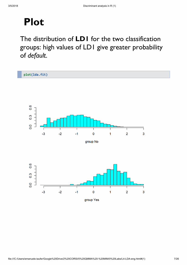
PlotThe distribution of LD1 for the two classificationgroups: high values of LD1 give greater probabilityof default.

plot(lda.fit)



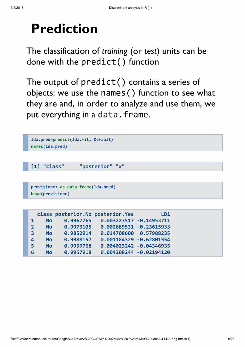
PredictionThe classification of training (or test) units can bedone with the predict() function

The output of predict() contains a series ofobjects: we use the names() function to see whatthey are and, in order to analyze and use them, weput everything in a data.frame.

lda.pred=predict(lda.fit, Default) names(lda.pred)

[1] "class" "posterior" "x"

previsione<-as.data.frame(lda.pred) head(previsione)

class posterior.No posterior.Yes LD1 1 No 0.9967765 0.003223517 -0.14953711 2 No 0.9973105 0.002689531 -0.23615933 3 No 0.9852914 0.014708600 0.57988235 4 No 0.9988157 0.001184329 -0.62801554 5 No 0.9959768 0.004023242 -0.04346935 6 No 0.9957918 0.004208244 -0.02194120



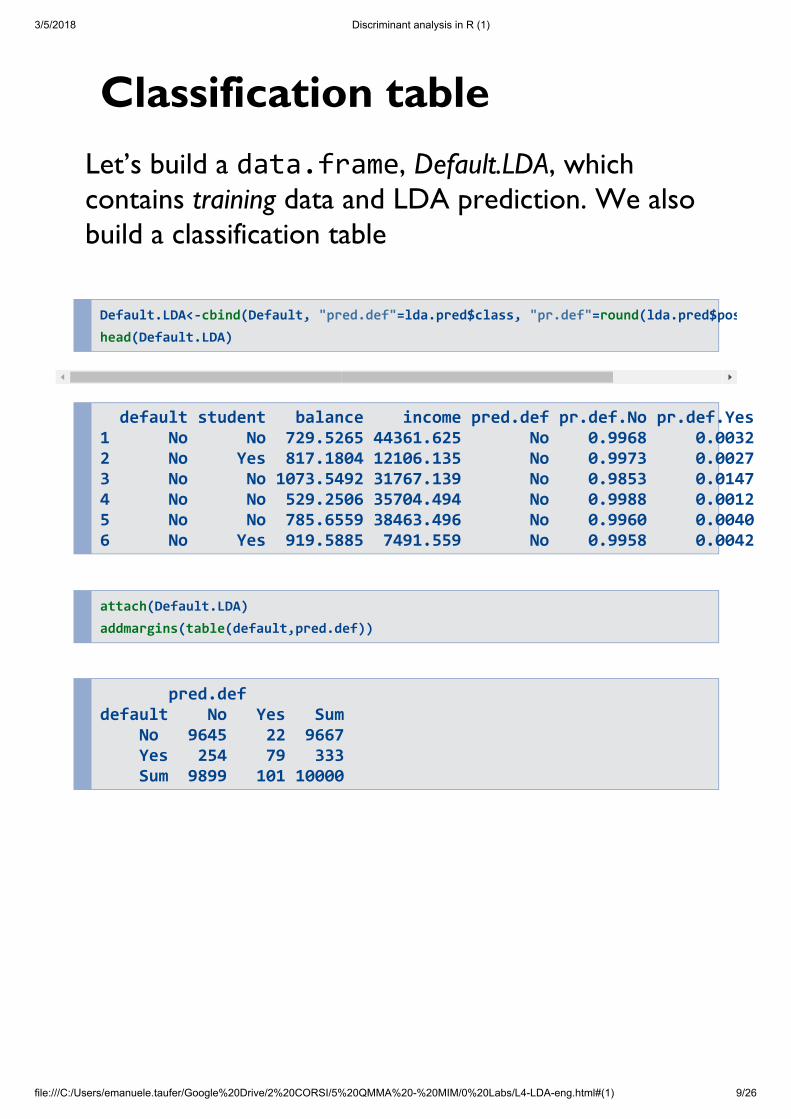
Classification tableLet’s build a data.frame, Default.LDA, whichcontains training data and LDA prediction. We alsobuild a classification table

default student balance income pred.def pr.def.No pr.def.Yes1 No No 729.5265 44361.625 No 0.9968 0.00322 No Yes 817.1804 12106.135 No 0.9973 0.00273 No No 1073.5492 31767.139 No 0.9853 0.01474 No No 529.2506 35704.494 No 0.9988 0.00125 No No 785.6559 38463.496 No 0.9960 0.00406 No Yes 919.5885 7491.559 No 0.9958 0.0042

attach(Default.LDA) addmargins(table(default,pred.def))

pred.def default No Yes Sum No 9645 22 9667 Yes 254 79 333 Sum 9899 101 10000

Default.LDA<-cbind(Default, "pred.def"=lda.pred$class, "pr.def"=round(lda.pred$poshead(Default.LDA)



Change the classificationcriterion

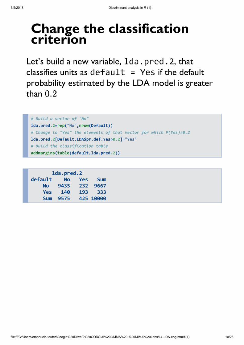
Let’s build a new variable, lda.pred.2, thatclassifies units as default = Yes if the defaultprobability estimated by the LDA model is greaterthan

# Build a vector of "No" lda.pred.2=rep("No",nrow(Default)) # Change to "Yes" the elements of that vector for which P(Yes)>0.2 lda.pred.2[Default.LDA$pr.def.Yes>0.2]="Yes" # Build the classification table addmargins(table(default,lda.pred.2))

lda.pred.2 default No Yes Sum No 9435 232 9667 Yes 140 193 333 Sum 9575 425 10000

0.2



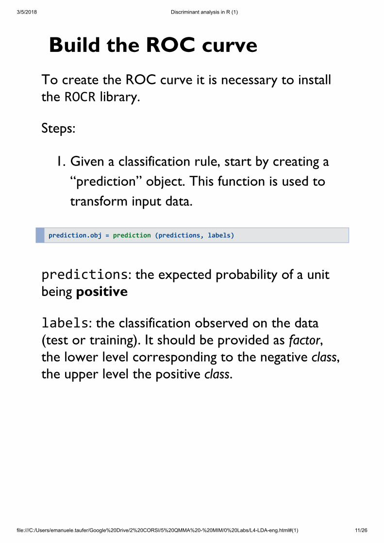
Build the ROC curveTo create the ROC curve it is necessary to installthe ROCR library.

Steps:

1. Given a classification rule, start by creating a“prediction” object. This function is used totransform input data.

prediction.obj = prediction (predictions, labels)

predictions: the expected probability of a unitbeing positive

labels: the classification observed on the data(test or training). It should be provided as factor,the lower level corresponding to the negative class,the upper level the positive class.



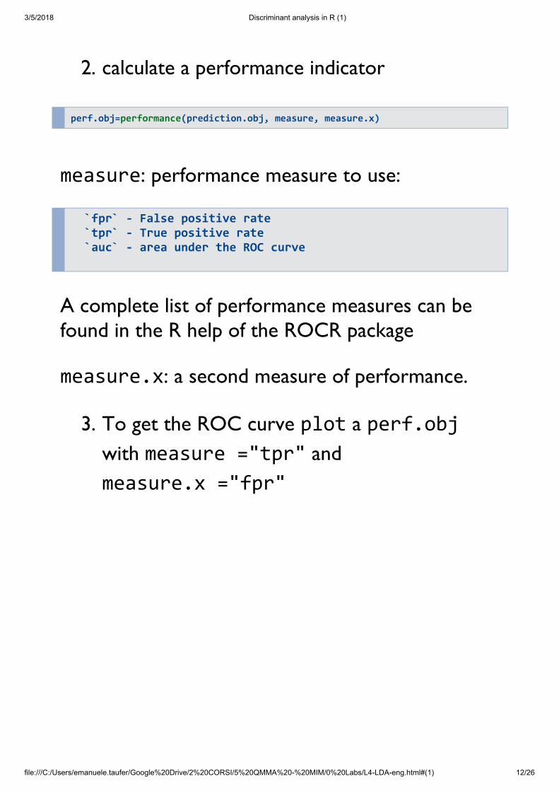
2. calculate a performance indicator

perf.obj=performance(prediction.obj, measure, measure.x)

measure: performance measure to use:

`fpr` - False positive rate `tpr` - True positive rate `auc` - area under the ROC curve

A complete list of performance measures can befound in the R help of the ROCR package

measure.x: a second measure of performance.

3. To get the ROC curve plot a perf.objwith measure ="tpr" andmeasure.x ="fpr"



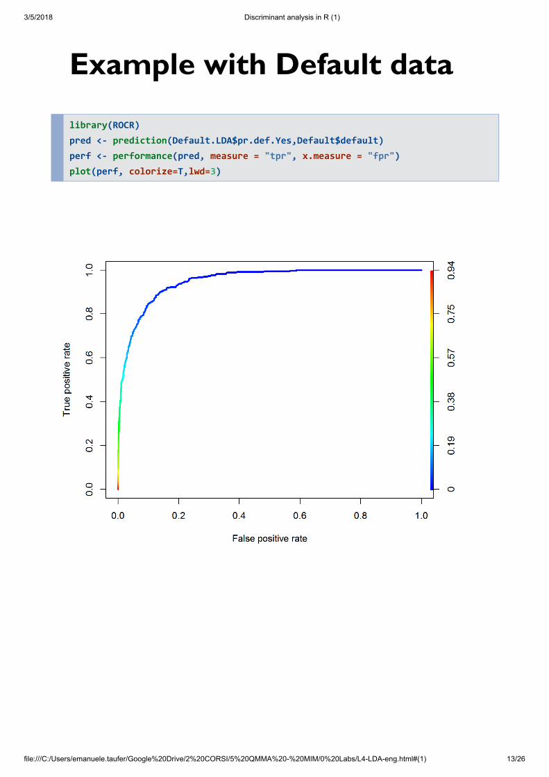
Example with Default data

library(ROCR) pred <- prediction(Default.LDA$pr.def.Yes,Default$default) perf <- performance(pred, measure = "tpr", x.measure = "fpr") plot(perf, colorize=T,lwd=3)



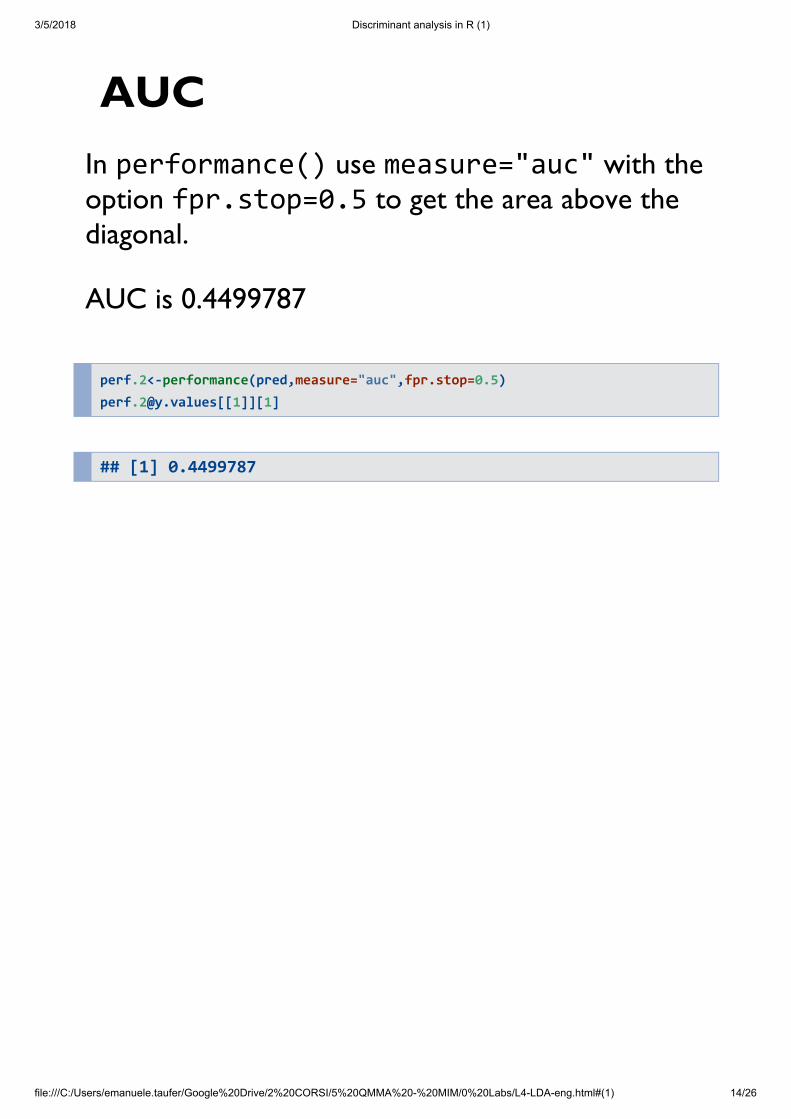
AUCIn performance() use measure="auc" with theoption fpr.stop=0.5 to get the area above thediagonal.

AUC is 0.4499787

perf.2<-performance(pred,measure="auc",fpr.stop=0.5) [email protected][[1]][1]

## [1] 0.4499787



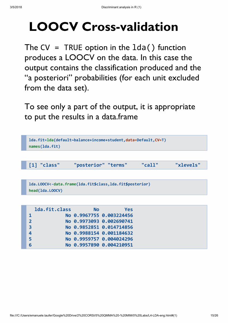
LOOCV Cross-validationThe CV = TRUE option in the lda() functionproduces a LOOCV on the data. In this case theoutput contains the classification produced and the“a posteriori” probabilities (for each unit excludedfrom the data set).

To see only a part of the output, it is appropriateto put the results in a data.frame

lda.fit=lda(default~balance+income+student,data=Default,CV=T) names(lda.fit)

[1] "class" "posterior" "terms" "call" "xlevels"

lda.LOOCV<-data.frame(lda.fit$class,lda.fit$posterior) head(lda.LOOCV)

lda.fit.class No Yes 1 No 0.9967755 0.003224456 2 No 0.9973093 0.002690741 3 No 0.9852851 0.014714856 4 No 0.9988154 0.001184632 5 No 0.9959757 0.004024296 6 No 0.9957890 0.004210951



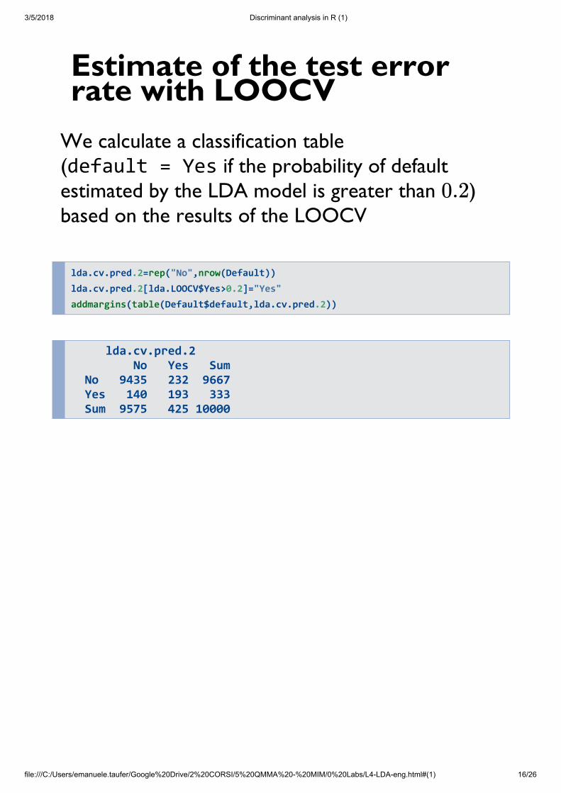
Estimate of the test errorrate with LOOCV

We calculate a classification table(default = Yes if the probability of defaultestimated by the LDA model is greater than )based on the results of the LOOCV

lda.cv.pred.2=rep("No",nrow(Default)) lda.cv.pred.2[lda.LOOCV$Yes>0.2]="Yes" addmargins(table(Default$default,lda.cv.pred.2))

lda.cv.pred.2 No Yes Sum No 9435 232 9667 Yes 140 193 333 Sum 9575 425 10000

0.2



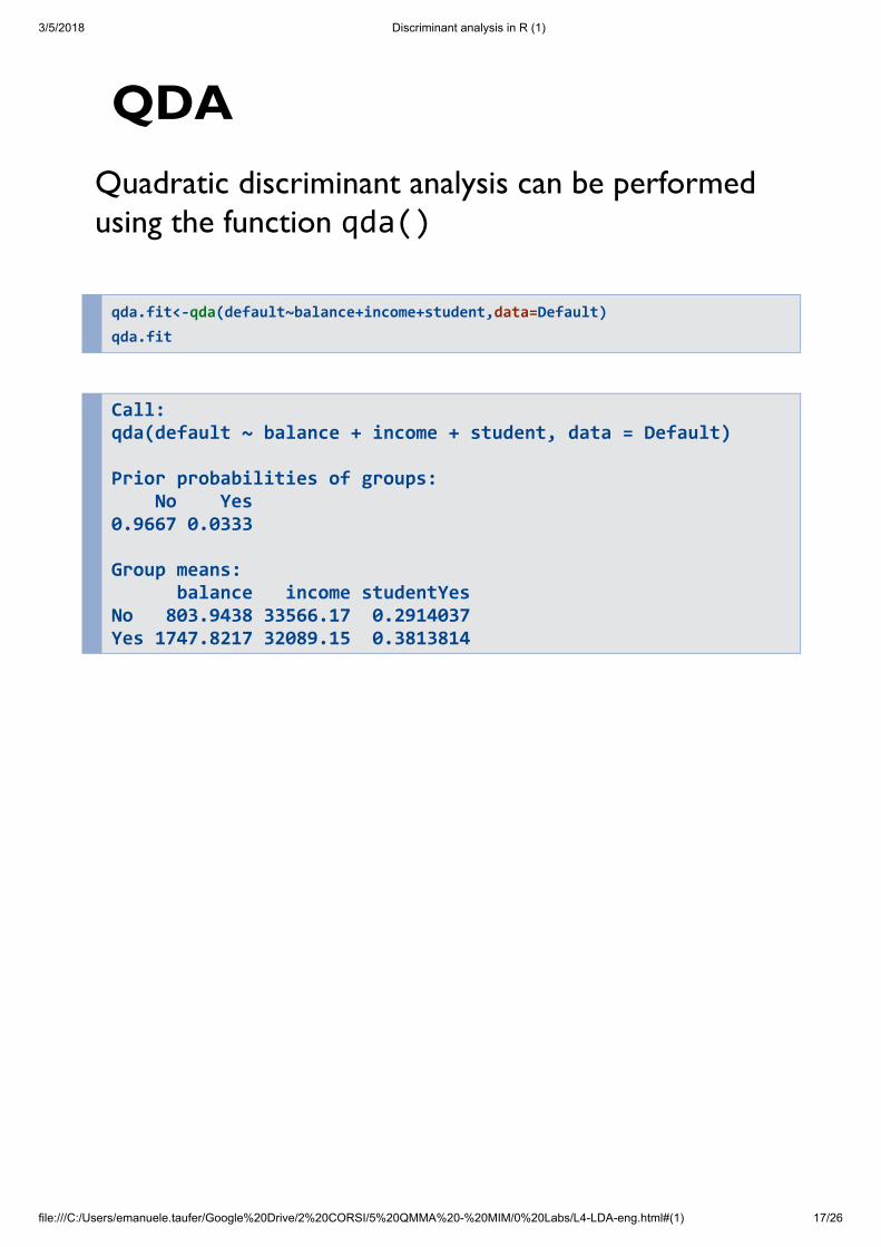
QDAQuadratic discriminant analysis can be performedusing the function qda()

qda.fit<-qda(default~balance+income+student,data=Default) qda.fit

Call: qda(default ~ balance + income + student, data = Default) Prior probabilities of groups: No Yes 0.9667 0.0333 Group means: balance income studentYes No 803.9438 33566.17 0.2914037 Yes 1747.8217 32089.15 0.3813814



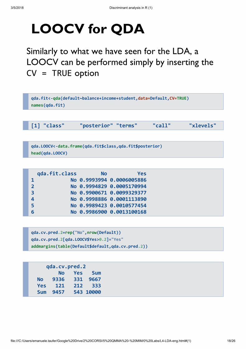
LOOCV for QDASimilarly to what we have seen for the LDA, aLOOCV can be performed simply by inserting theCV = TRUE option

qda.fit<-qda(default~balance+income+student,data=Default,CV=TRUE) names(qda.fit)

[1] "class" "posterior" "terms" "call" "xlevels"

qda.LOOCV<-data.frame(qda.fit$class,qda.fit$posterior) head(qda.LOOCV)

qda.fit.class No Yes 1 No 0.9993994 0.0006005886 2 No 0.9994829 0.0005170994 3 No 0.9900671 0.0099329377 4 No 0.9998886 0.0001113890 5 No 0.9989423 0.0010577454 6 No 0.9986900 0.0013100168

qda.cv.pred.2=rep("No",nrow(Default)) qda.cv.pred.2[qda.LOOCV$Yes>0.2]="Yes" addmargins(table(Default$default,qda.cv.pred.2))

qda.cv.pred.2 No Yes Sum No 9336 331 9667 Yes 121 212 333 Sum 9457 543 10000



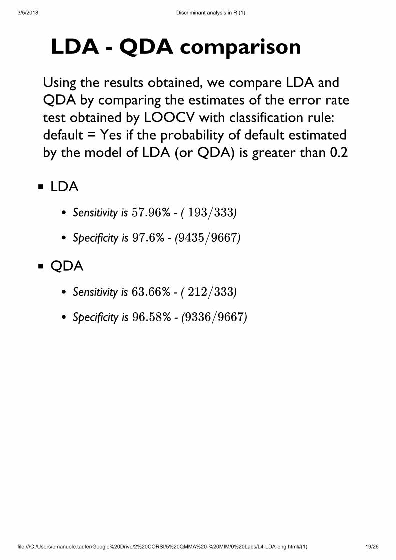
LDA - QDA comparisonUsing the results obtained, we compare LDA andQDA by comparing the estimates of the error ratetest obtained by LOOCV with classification rule:default = Yes if the probability of default estimatedby the model of LDA (or QDA) is greater than 0.2

LDA

Sensitivity is % - ( )

Specificity is % - ( )

QDA

Sensitivity is % - ( )

Specificity is % - ( )

57.96 193/333

97.6 9435/9667

63.66 212/333

96.58 9336/9667



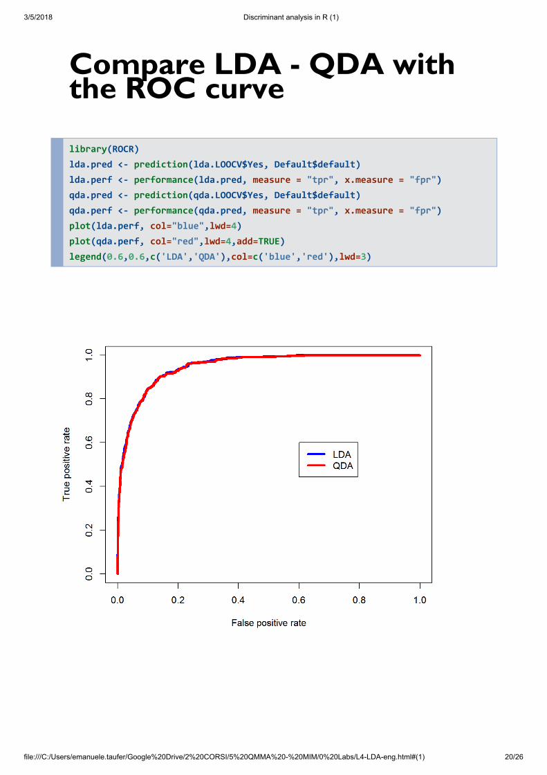
Compare LDA - QDA withthe ROC curve

library(ROCR) lda.pred <- prediction(lda.LOOCV$Yes, Default$default) lda.perf <- performance(lda.pred, measure = "tpr", x.measure = "fpr") qda.pred <- prediction(qda.LOOCV$Yes, Default$default) qda.perf <- performance(qda.pred, measure = "tpr", x.measure = "fpr") plot(lda.perf, col="blue",lwd=4) plot(qda.perf, col="red",lwd=4,add=TRUE) legend(0.6,0.6,c('LDA','QDA'),col=c('blue','red'),lwd=3)



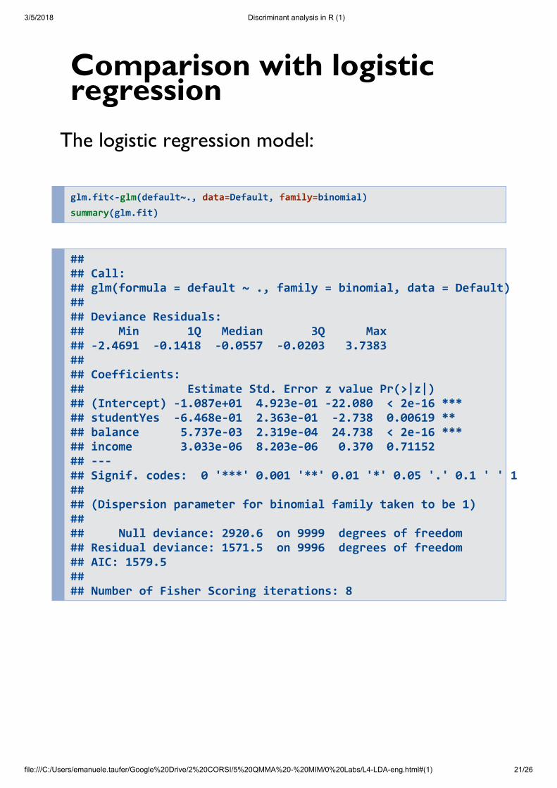
Comparison with logisticregression

The logistic regression model:

glm.fit<-glm(default~., data=Default, family=binomial) summary(glm.fit)

## ## Call: ## glm(formula = default ~ ., family = binomial, data = Default) ## ## Deviance Residuals: ## Min 1Q Median 3Q Max ## -2.4691 -0.1418 -0.0557 -0.0203 3.7383 ## ## Coefficients: ## Estimate Std. Error z value Pr(>|z|) ## (Intercept) -1.087e+01 4.923e-01 -22.080 < 2e-16 *** ## studentYes -6.468e-01 2.363e-01 -2.738 0.00619 ** ## balance 5.737e-03 2.319e-04 24.738 < 2e-16 *** ## income 3.033e-06 8.203e-06 0.370 0.71152 ## --- ## Signif. codes: 0 '***' 0.001 '**' 0.01 '*' 0.05 '.' 0.1 ' ' 1 ## ## (Dispersion parameter for binomial family taken to be 1) ## ## Null deviance: 2920.6 on 9999 degrees of freedom ## Residual deviance: 1571.5 on 9996 degrees of freedom ## AIC: 1579.5 ## ## Number of Fisher Scoring iterations: 8



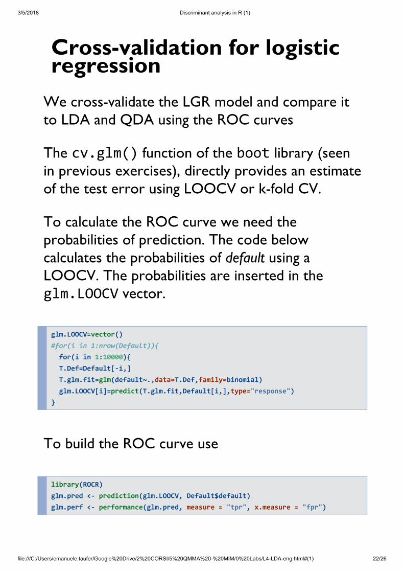
Cross-validation for logisticregression

We cross-validate the LGR model and compare itto LDA and QDA using the ROC curves

The cv.glm() function of the boot library (seenin previous exercises), directly provides an estimateof the test error using LOOCV or k-fold CV.

To calculate the ROC curve we need theprobabilities of prediction. The code belowcalculates the probabilities of default using aLOOCV. The probabilities are inserted in theglm.LOOCV vector.

glm.LOOCV=vector() #for(i in 1:nrow(Default)){ for(i in 1:10000){ T.Def=Default[-i,] T.glm.fit=glm(default~.,data=T.Def,family=binomial) glm.LOOCV[i]=predict(T.glm.fit,Default[i,],type="response") }

To build the ROC curve use

library(ROCR) glm.pred <- prediction(glm.LOOCV, Default$default) glm.perf <- performance(glm.pred, measure = "tpr", x.measure = "fpr")





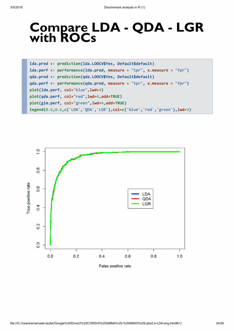
Compare LDA - QDA - LGRwith ROCs

lda.pred <- prediction(lda.LOOCV$Yes, Default$default) lda.perf <- performance(lda.pred, measure = "tpr", x.measure = "fpr") qda.pred <- prediction(qda.LOOCV$Yes, Default$default) qda.perf <- performance(qda.pred, measure = "tpr", x.measure = "fpr") plot(lda.perf, col="blue",lwd=4) plot(qda.perf, col="red",lwd=4,add=TRUE) plot(glm.perf, col="green",lwd=4,add=TRUE) legend(0.6,0.6,c('LDA','QDA','LGR'),col=c('blue','red','green'),lwd=3)



AUCThe AUC for the three models, calculated on thecross-validated data with LOOCV, are:

LDA: 0.4495681

QDA: 0.4487009

RLG: 0.4493764

In this case, three models are equivalent.

The choice of which model to use can be based onpurely personal considerations



ReferencesAn Introduction to Statistical Learning, withapplications in R. (Springer, 2013)

Tobias Sing, Oliver Sander, Niko Beerenwinkel,Thomas Lengauer. ROCR: visualizing classifierperformance in R. Bioinformatics 21(20):3940-3941(2005).

Documents

D i s cr i m i n a n t a n a l y s i s i n R QM M A