Embed Size (px)
Citation preview

CZECH TECHNICAL UNIVERSITY IN PRAGUE
DOCTORAL THESIS


Risk management of tunnel construction projects
Doctoral Thesis
Ing. Olga Špačková
Prague, June 2012
Ph.D. Programme: Civil Engineering
Supervisor: Prof. Ing. Jiří Šejnoha, DrSc.
Supervisor - specialist: Prof. Dr. Daniel Straub
CZECH TECHNICAL UNIVERSITY IN PRAGUE
Faculty of Civil Engineering
Department of Mechanics


To the memory of my father

v
Estimates of uncertainties and risks of the construction process are essential information for
decision-making in infrastructure projects. The construction process is affected by different types of
uncertainties. We can distinguish between the common variability of the construction process and
the uncertainty on occurrence of extraordinary events, also denoted as failures of the construction
process. In tunnel construction, a significant part of the uncertainty results from the unknown
geotechnical conditions. The construction performance is further influenced by human and
organizational factors, whose effect is not known in advance. All these uncertainties should be
taken into account when modelling the uncertainty and risk of the tunnel construction.
For reliable predictions, it is essential to realistically estimate the parameters of the probabilistic
model. At present, such estimates mostly rely on expert judgement. However, these can be strongly
biased and unreliable. Therefore, the expert estimates should be supported by analysis of data from
previous projects.
This thesis attempts to address these issues. First, it introduces a simple probabilistic model for
the estimation of the delay due to occurrence of construction failures. The model is applied to a case
study, which demonstrates, how the probabilistic estimate of construction delay can be used for
assessing the risk and for making decisions.
Second, advanced model including both the common variability and construction failures using
Dynamic Bayesian Networks (DBNs) is presented. This model takes over some modelling
procedures from existing models but it extends the scope of the modelled uncertainties. The model
is applied to two case studies for the estimation of tunnel construction time. It is demonstrated, how
observations from the tunnel construction process can be included to continuously update the
prediction of excavation time.
Third, an efficient algorithm for the evaluation of the proposed DBN is developed. A
modification to the existing Frontier algorithm is suggested, denoted as modified Frontier
algorithm. This new algorithm is efficient for evaluating DBNs with cumulative variables.
Fourth, performance data from tunnels constructed in the past are analysed. The data motivates
the development of a novel combined probability distribution to describe the excavation
performance. In addition, the probability of construction failure and the delay caused by such
failures is estimated using databases available in the literature. Additionally, a brief database of
tunnel projects and tunnel construction failures from the Czech Republic is compiled. The database
includes basic information on all tunnels, which have been constructed in the Czech Republic since
1989. The database of failures, which occurred in the analysed tunnels, contains 17 events, mostly
cave-in collapses.
The models presented in this thesis are applied to the estimation of tunnel construction time. The
construction costs can be assessed analogously by replacing the time variables with cost variables.
The costs can also be modelled as a function of the construction time.
The statistical analysis of data presented in the thesis provides a valuable input for probabilistic
prediction of construction time in infrastructure projects. The results of the case studies seem to
realistically reflect the uncertainty of the construction time estimates.
Abstract

vii
Zhodnocení nejistot a rizik stavebního procesu je základní informací pro rozhodování v rámci
plánování a řízení infrastrukturních projektů. Stavební proces je ovlivněn různými typy nejistot.
Můžeme rozlišit mezi běžnou variabilitou stavebního procesu a možnou realizací výjimečných
událostí. V tunelových stavbách pramení významná část nejistot z neznámých geotechnických
podmínek. Postup stavby je dále ovlivněn lidskými a organizačními faktory, jejichž efekt není
v předstihu znám. Všechny tyto nejistoty by měly být při modelování nejistot a rizik tunelové ražby
zohledněny.
Mají-li být predikce průběhu tunelové stavby spolehlivé, je nutné realisticky odhadnout
parametry pravděpodobnostního modelu, jako je např. jednotkový čas nebo pravděpodobnost
výjimečné události. V dosavadních aplikacích byly parametry určovány v naprosté většině případů
expertním odhadem. Expertní odhady však mohou být značně subjektivní a zkreslené, měly by
proto být podepřeny analýzou dat z dříve realizovaných staveb tunelů.
Tato dizertační práce se snaží odpovědět na výše zmíněné problémy. Zaprvé je představen
jednoduchý pravděpodobnostní model pro predikci zdržení stavby v důsledku výjimečných
událostí. Příklad, na kterém je model aplikován, demonstruje, jak může být pravděpodobnostní
odhad zdržení stavby použit pro kvantifikaci rizika a pro rozhodování o výběru technologie ražby.
Zadruhé je navržen pokročilý model, který zahrnuje jak běžnou variabilitu stavebního procesu,
tak potenciální realizaci výjimečných událostí. Model využívá dynamických bayesovských sítí,
přejímá některé procedury z existujících modelů, ale rozšiřuje spektrum modelovaných nejistot.
Model je aplikován na dvou příkladech pro odhad doby ražby tunelu. Apriorní odhad je
aktualizován po započetí ražby na základě pozorování dosahovaných stavebních výkonů.
Zatřetí je navržen efektivní algoritmus pro vyhodnocení tohoto modelu, který umožňuje rychlý
výpočet doby ražby včetně její průběžné aktualizace. Algoritmus spočívá v modifikaci existujícího
algoritmu známého pod názvem „Frontier algorithm“ a je vhodný pro vyhodnocování dynamických
bayesovských sítí, které obsahují kumulativní (součtové) náhodné veličiny.
Začtvrté jsou analyzována data z postupu tunelových staveb realizovaných v minulosti. Na
základě této analýzy bylo navrženo nové kombinované pravděpodobnostní rozdělení, které dobře
reprezentuje skutečný výkon stavby. Na základě existujících databází havárií tunelů byly
analyzovány četnost výjimečných událostí a zdržení těmito událostmi způsobená. Dále byla
vytvořena stručná databáze tunelů postavených v České Republice po roce 1989 a databáze 17
výjimečných událostí, ke kterým při jejich stavbě došlo.
Navržené pravděpodobnostní modely jsou použity pro predikci doby výstavby. Stavební
náklady mohou být odhadnuty analogicky záměnou proměnných reprezentujících čas za nákladové
proměnné. Stavební náklady mohou být také modelovány jako funkce doby výstavby.
Prezentované výsledky analýzy dat jsou cenným podkladem pro odhad doby výstavby
budoucích tunelových projektů i dalších typů liniových staveb. Výsledky případových studií
dokládají, že navržené modely realisticky reflektují nejistoty spojené s odhadem doby výstavby.
Abstrakt


ix
First of all, I would like to express my deepest thanks to Prof. Jiří Šejnoha, who made me interested
in the topic of risk analysis and who supported me continuously during my work in this challenging
field.
I would also like to sincerely thank my second supervisor Prof. Daniel Straub for his support,
guidance and inspiration, which essentially influenced the direction of my life and achievements of
my work.
Special thanks belong to Prof. Milík Tichý and Prof. Kazuyoshi Nishijima, who agreed to act as
opponents of this thesis.
I would like to thank sincerely my numerous advisors and supporters: Prof. Daniela Jarušková
and Prof. Jiří Barták from my home university, for their advices in statistics and geotechnics. Many
thanks should be expressed to Doc. Alexandr Rozsypal, Ing. Tomáš Ebermann, Ing. Ondřej
Kostohryz and Ing. Václav Veselý from Arcadis Geotechnika for the fruitful collaboration on the
research projects and for providing me with data. I also thank very much the tunnelling specialists,
who devoted their time to discuss with me the practical issues of the tunnel construction: Dr. Radko
Bucek (Mott MacDonald, Prague), Ing. Martin Srb (D2Consult, Prague), Ing. Miroslav Vlk
(Metrostav, Prague), Dr. Alexandr Butovič (Satra, Prague), Ing. Tobias Nevrly (TUM, Munich),
Ing. Miroslav Bocák, Ing. Pavek Krotil and Mgr. Hocký (Czech railway administration - SŽDC). Many thanks to all my colleagues and friends for their support and for the great time I had
during my PhD studies. Unfortunately it is impossible to name everybody, so at least some: Anička
Kučerová, Zuzka Vitingerová, Jan Sýkora, Jan Vorel, Richard Valenta, Jan Novák, Tomáš Janda,
Patty Papakosta, Simona Miraglia, Giulio Cottone and Johannes Fischer.
Finally, I would like to thank my mother and grandmother for their endless love and support.
This work was supported by project No. 1M0579 (CIDEAS research centre) of the Ministry of
Education, Youth and Sports of the Czech Republic, by project No. TA01030245 of the Technology
Agency of the Czech Republic and by project No. 103/09/2016 of the Czech Science Foundation.
Furthermore, this work has received financial support from the internal grant projects CTU0907411
and SGS10/020/OHK1/1T/11 at the Czech Technical University in Prague. Additional support of
my stay at the university in Munich by DAAD and Bayhost is gratefully acknowledged.
Olga Špačková
June, 2012
Acknowledgements

xi
Abstract ............................................................................................................................................... v
Abstrakt ............................................................................................................................................ vii
Acknowledgements ........................................................................................................................... ix
Contents ............................................................................................................................................. xi
1 Introduction .................................................................................................................................. 1
1.1 Research objectives ..................................................................................................................... 2
1.2 Thesis outline .............................................................................................................................. 3
2 Tunnel projects and risk management ....................................................................................... 5
2.1 Tunnel project planning and decision making ............................................................................ 6
2.2 Tunnel construction ..................................................................................................................... 8
2.2.1 Conventional tunnelling ....................................................................................................... 8
2.2.2 Mechanized tunnelling ....................................................................................................... 10
2.2.3 Cut & cover tunnelling ....................................................................................................... 12
2.3 Geotechnical classification systems .......................................................................................... 12
2.3.1 Rock Mass Rating (RMR) .................................................................................................. 13
2.3.2 Q-system ............................................................................................................................. 14
2.3.3 Czech classification - QTS index ....................................................................................... 14
2.3.4 Qualitative and project specific classification systems ...................................................... 14
2.3.5 Comparison of the classification systems .......................................................................... 15
2.4 Estimation of construction time and costs ................................................................................. 16
2.5 Tunnel construction failures ...................................................................................................... 17
2.6 Risk management ...................................................................................................................... 19
2.6.1 Risk management process .................................................................................................. 20
2.6.2 Risk management of construction projects ........................................................................ 21
2.6.3 Risk and procurement of tunnel projects ............................................................................ 21
2.6.4 Risk and insurance of tunnel projects ................................................................................ 22
2.7 Uncertainties in the tunnel projects ........................................................................................... 22
Contents
xii
2.8 Summary ................................................................................................................................... 23
3 Analysis of tunnel construction risk ......................................................................................... 25
3.1 Qualitative risk analysis ............................................................................................................ 26
3.2 Quantitative analysis of uncertainty and risk ............................................................................ 27
3.3 Introduction to selected methods for uncertainty and risk modelling ...................................... 29
3.3.1 Fault tree analysis (FTA) ................................................................................................... 29
3.3.2 Event tree analysis (ETA) .................................................................................................. 30
3.3.3 Bernoulli process, Binomial distribution and Poisson process .......................................... 30
3.3.4 Markov process .................................................................................................................. 32
3.3.5 Bayesian networks ............................................................................................................. 33
3.3.6 Dynamic Bayesian networks ............................................................................................. 34
3.3.7 Utility theory in decision analysis ..................................................................................... 35
3.4 Summary ................................................................................................................................... 36
4 Model of delay due to tunnel construction failures and estimate of associated risk ........... 39
4.1 Modelling delay due to failures - methodology ........................................................................ 39
4.1.1 Number of failures ............................................................................................................. 39
4.1.2 Estimation of damages ....................................................................................................... 41
4.2 Application example 1: Risk of construction failure in tunnel TUN3 ...................................... 42
4.2.1 Number of failures ............................................................................................................. 43
4.2.2 Consequences .................................................................................................................... 44
4.2.3 Risk quantification ............................................................................................................. 47
4.2.4 Alternative tunnelling technology, decision about the optimal technology ...................... 49
4.3 Summary and discussion .......................................................................................................... 49
5 Dynamic Bayesian network (DBN) model of tunnel construction process ........................... 51
5.1 Generic DBN model ................................................................................................................. 52
5.1.1 Geotechnical conditions ..................................................................................................... 53
5.1.2 Construction performance ................................................................................................. 54
5.1.3 Extraordinary events .......................................................................................................... 55
5.1.4 Length of segment represented by a slice of DBN ............................................................ 55
5.2 Specific DBN model ................................................................................................................. 55
5.2.1 Zone ................................................................................................................................... 57
5.2.2 Rock class .......................................................................................................................... 57
5.2.3 Overburden and Ground class ........................................................................................... 58
5.2.4 Variables describing construction performance ................................................................ 58
5.2.5 Failure mode ...................................................................................................................... 59
5.2.6 Number of failures ............................................................................................................. 59
5.2.7 Construction time ............................................................................................................... 59
5.3 Application example 2: Dolsan A tunnel ................................................................................. 60
5.3.1 Numerical inputs ................................................................................................................ 61
5.3.2 Results ................................................................................................................................ 64
5.4 Summary and discussion .......................................................................................................... 67
6 Algorithms for evaluating the DBN ......................................................................................... 69
6.1 Introduction to inference in Bayesian networks ....................................................................... 69
6.1.1 Inferring unobserved variables .......................................................................................... 70
Introduction xiii
6.1.2 Parameter learning .............................................................................................................. 73
6.1.3 Discretization of random variables .................................................................................... 75
6.1.4 Principles of the Frontier algorithm ................................................................................... 75
6.2 Evaluation of the DBN .............................................................................................................. 77
6.2.1 Discretization of random variables .................................................................................... 77
6.2.2 Elimination of nodes .......................................................................................................... 78
6.2.3 Modified Frontier algorithm ............................................................................................... 79
6.2.4 Updating ............................................................................................................................. 82
6.2.5 Adaptation of the model parameters .................................................................................. 82
6.2.6 Calculation of total time ..................................................................................................... 83
6.3 Summary and discussion ........................................................................................................... 83
7 Analysis of tunnel construction data for learning the model parameters ............................. 85
7.1 Unit time .................................................................................................................................... 86
7.1.1 Advance rate and unit time as a stochastic process ............................................................ 86
7.1.2 Data .................................................................................................................................... 88
7.1.3 Statistical analysis .............................................................................................................. 91
7.1.4 Correlation analysis ............................................................................................................ 94
7.2 Extraordinary events ................................................................................................................. 96
7.2.1 Delay caused by a failure ................................................................................................... 96
7.2.2 Failure rate .......................................................................................................................... 97
7.3 Application example 3: TUN3 ................................................................................................ 100
7.3.1 Definition of the random variables and numerical inputs ................................................ 102
7.3.2 Results .............................................................................................................................. 104
7.4 Summary and discussion ......................................................................................................... 110
8 Conclusions and outlook .......................................................................................................... 113
8.1 Main contributions of the thesis .............................................................................................. 114
8.2 Outlook .................................................................................................................................... 115
Abbreviations .................................................................................................................................. 117
Bibliography ................................................................................................................................... 119
Annexes ........................................................................................................................................... 131
ANNEX 1: Basics of probability theory, notation ........................................................................... 133
ANNEX 2: Inputs for application example 2: Dolsan A tunnel ...................................................... 137
ANNEX 3: Validation of the DBN model through comparison with the DAT model + sensitivity
analysis ............................................................................................................................................. 139
ANNEX 4: Validation of the modified Frontier algorithm, comparison of computational efficiency
.......................................................................................................................................................... 143
ANNEX 5: Overview of tunnels constructed in the Czech Rep. after 1989 and database of tunnel
construction failures ......................................................................................................................... 147
ANNEX 6: Statistical analysis of performance data ........................................................................ 151
ANNEX 7: Updating parameters of unit time .................................................................................. 159

1
In developed countries, investments into the transportation infrastructure (construction and
maintenance of roads, railways etc.) vary in the interval from 0.5% to 1.5% of the GDP; new
construction corresponds to approximately two thirds of this amount (Banister and Berechman,
2000; U.S. Department of transportation, 2004; International Transport Forum - OECD, 2011). In
developing countries, the share of the GDP may be significantly higher, up to 6% (UN ESCAP,
2006). When including also water, energy and communication infrastructure, the global investments
to infrastructure are assessed roughly ass 2.5% of the world GDP (OECD, 2007). The optimization
of the design and construction of the infrastructure can therefore bring significant benefits to the
society.
To be successful, a project must meet financial, technical and safety requirements and it must
fulfil a time schedule. The criteria of project success from the point of view of different
stakeholders can be contradicting and finding an optimal solution is a challenging task. Many
decisions must be made regarding design, project financing and type of contract. These decisions
are made under high uncertainty, such as uncertainty in construction cost, time of completion,
impact on third party property or maintenance costs. Assessment of these uncertainties is crucial for
making the right decisions. Often, the solutions that seem to be cheaper and faster based on
deterministic estimates, are associated with higher uncertainties and risks. Making decisions based
on deterministic values is therefore insufficient.
This thesis aims at developing models for quantification of uncertainties in the construction
process of linear infrastructure. Specifically, the models are developed for probabilistic assessment
of tunnel construction. Tunnels were selected because they represent a costly part of the
infrastructure and because the progress of their construction is highly uncertain. Compared to other
types of linear infrastructure, this additional uncertainty arises from the unpredictable geotechnical
environment, where the tunnels are built (Staveren, 2006). The models developed for tunnel
construction can be applied also to other types of linear infrastructure (e.g. roads or railways) as
shown for example in Moret (2011); in such a case, modelling of geotechnical uncertainties can be
simplified or neglected.
1 Introduction
2 Introduction
There are only few methods and models for quantification of uncertainty in construction time
and cost prediction for infrastructure in general (Flyvbjerg, 2006), or for tunnels in particular, e.g.
the Decision Aids for Tunnelling (DAT) developed at MIT in group of Prof. Einstein (e.g. Einstein,
1996), an analytical model presented by Isaksson and Stille (2005) or a model combining Bayesian
networks and Monte Carlo simulation proposed by Steiger (2009). Probabilistic models have not
been widely accepted in the practice so far. A first reason is that there was not real demand for the
quantitative modelling of uncertainties and risk, because decision makers were not used to work
with such information. A second reason is that the existing models often did not provide a realistic
estimate of the uncertainties and they therefore did not gain acceptance among the practitioners.
However, this situation seems to be changing in the recent years and both the demand and the
reliability of the model results have increased.
1.1 Research objectives
The objective of this thesis is to provide tools for the analysis of tunnel construction uncertainties
and risks. The particular aims are:
To propose a methodology that allows estimating the delay of tunnel construction due to failures on a probabilistic basis. The estimate might be used as a supplement to the deterministic estimates of construction time.
To illustrate the use of the probabilistic estimate of construction delay for quantification of risk and for making decisions.
To develop an advanced model that can realistically assess the overall uncertainty of the tunnel construction time (cost) estimates, including both the common variability of the construction process and the occurrence of failures (extraordinary events).
To demonstrate the updating of the estimates with the observed performance after the construction starts.
To develop an efficient algorithm for evaluation of the models in real time.
Besides development of the probabilistic models, the thesis aims at gathering and analysing
performance data from the constructed tunnels. Based on this analysis, the parameters of the
probabilistic models (and not only those presented in this thesis) may be estimated more
realistically.
The analysis of data describes both:
The common variability of the construction performance;
The extraordinary events and delays caused by these events.
A brief database of tunnel projects and tunnel construction failures in the Czech Republic since 1990 is established. It supplements the existing databases of world tunnels failures.
Introduction 3
1.2 Thesis outline
The thesis is organized into eight chapters and seven annexes. The second and third chapters are
introductory:
The second chapter “Tunnel projects and risk management” answers the question, WHY we should
analyse uncertainties and risks of tunnel construction. It provides a brief introduction into the topic
of tunnel projects and tunnel construction. The present practice of project planning and decision-
making is described. The concept of risk and its management is introduced.
The third chapter “Analysis of tunnel construction” addresses the question, HOW we can analyse
uncertainty and risk. The state-of-the-art in tunnel construction risk analysis is described; both
qualitative and quantitative approaches are discussed. Selected methods and models for
quantification of uncertainties and risk, which are used later in the thesis, are introduced.
Corresponding basic definitions and axioms of probabilistic modelling together with an overview of
the terminology and notation is provided in Annex 1.
The new findings are presented in chapters four to seven. The application of the new models is
demonstrated in three application examples. Two of the examples use a Czech tunnel denoted as
TUN 3, which is also included in the analysis of data. One of the examples uses a Korean tunnel
denoted as Dolsan A, this case study was taken from the literature (Min et al., 2003).
The fourth chapter “Model of delay due to tunnel construction failures and the estimate of
associated risk” introduces a simple probabilistic model for quantification of the delay caused by
extraordinary events by means of Poisson processes and Event Tree Analysis (ETA). The
application example 1 is presented using tunnel TUN3; the estimated delay is used for the
quantification of risk and for the selecting an optimal construction technology.
The fifth chapter “Dynamic Bayesian network (DBN) model of tunnel construction process”
introduces a complex probabilistic model for the prediction of tunnel construction time and costs. A
generic approach to the modelling is introduced. Furthermore, a specific model for the prediction of
construction time is discussed in detail. This model is applied to the case study of the Dolsan A
tunnel. The updating of the prediction with observed performance is demonstrated. The comparison
and validation of the new model with results of the original case study taken from Min (2003) is
provided in Annex 3.
The sixth chapter “Algorithms for the evaluation of the DBN” focuses on the probabilistic
modelling itself; it can be skipped by a reader, whose interest is in risk modelling of tunnel projects.
The chapter introduces the algorithms for inferring unobserved variables in the DBN and for
learning the parameters of the DBN. The procedure for evaluating the DBN for tunnel construction
is described in detail. A modification to the Frontier algorithm (Murphy, 2002) is proposed which is
efficient for evaluating DBNs with cumulative variables. A comparison of the performance of the
original and modified Frontier algorithm is presented in Annex 4.
The seventh chapter “Analysis of tunnel construction data for learning the model parameters”
presents methods for analysing performance data from projects constructed in the past. The
common variability of the construction process and the construction failures are studied separately.
The first is analysed using data from three Czech tunnels (full results of the analysis are given in
Annex 6), the later is based on analysis of larger databases of tunnels and tunnel construction
failures. The findings are applied to the case study of tunnel TUN3; prior estimates of the
4 Introduction
parameters are determined by an expert judgement supported by the data analysis, the predictions
are then updated with real observations.
Because the existing databases of tunnel construction failures do not contain the cases that occurred
in the Czech Republic, a database of tunnel projects and tunnel construction failures in the Czech
Republic in the years 1990-2012 was collected (Annex 5). The database includes only basic
information about the tunnels (e.g. type and length of the tunnel, time of construction) and
construction failures (e.g. consequences, taken measures). Additional information can be found in
the referred sources, which are available also in English.
The eighth chapter “Conclusions and outlook” summarizes the main achievements and conclusions
of the thesis and provides hints for future work.
5
With proceeding urbanization and increasing demands on life-quality, the importance of
underground infrastructure, including tunnels, is likely to increase in the future. Tunnels minimize
the impact of the infrastructure (e.g. road or railway) on the environment; they allow placing the
infrastructure in the cities under ground and thus improve the life quality of the inhabitants. Tunnels
also help to fulfil the increasing demands on the technical parameters of the infrastructure; the
modern roads and railways, to comply with the requirements on high design speed, must have
sweeping curves and gentle elevation. In a complicated terrain, this can often be gained only
through designing tunnels.
Tunnels are built in geotechnical conditions, which are not known with certainty before the
tunnel is constructed. Other uncertainties influencing the project success come from the human and
organizational factors. At present, the time and costs of the construction are commonly estimated on
the deterministic basis. This approach, however, is likely to lead to wrong decisions, because it
neglects the uncertainties of the estimates.
This chapter aims at introducing the context and motivation of the probabilistic models for the
estimation of tunnel construction time (or costs) presented later in this thesis. In Section 2.1, the
importance of the construction phase for the life of the tunnel project is demonstrated and the need
of probabilistic estimates of construction costs and time is discussed. The technologies of tunnel
construction are described in Section 2.2. Because the geology and its appropriate description are
decisive factors for tunnel design and construction, the commonly utilized geotechnical
classification systems are introduced in Section 2.3. Section 2.4 describes, how the estimates of
construction costs and time are done in the present practice. Section 2.5 discusses the failures of the
tunnel construction, i.e. events, which have relatively small probability but potentially huge impact
on the construction process. Section 2.6 focuses on risk management and its application in the
tunnel projects: The definition of risk is introduced; the generic risk management process is
described and implications of risk management for procurement and insurance of the tunnel project
are examined. Finally, the uncertainties in the tunnel project are discussed in Section 2.7.
2 Tunnel projects and risk
management
6 Tunnel projects and risk management
2.1 Tunnel project planning and decision making
In early phase of planning of an infrastructure project, several alternatives are commonly
considered. These alternatives can include different layouts of the infrastructure, different
combinations of tunnel and bridges or different construction technologies. The early design phase
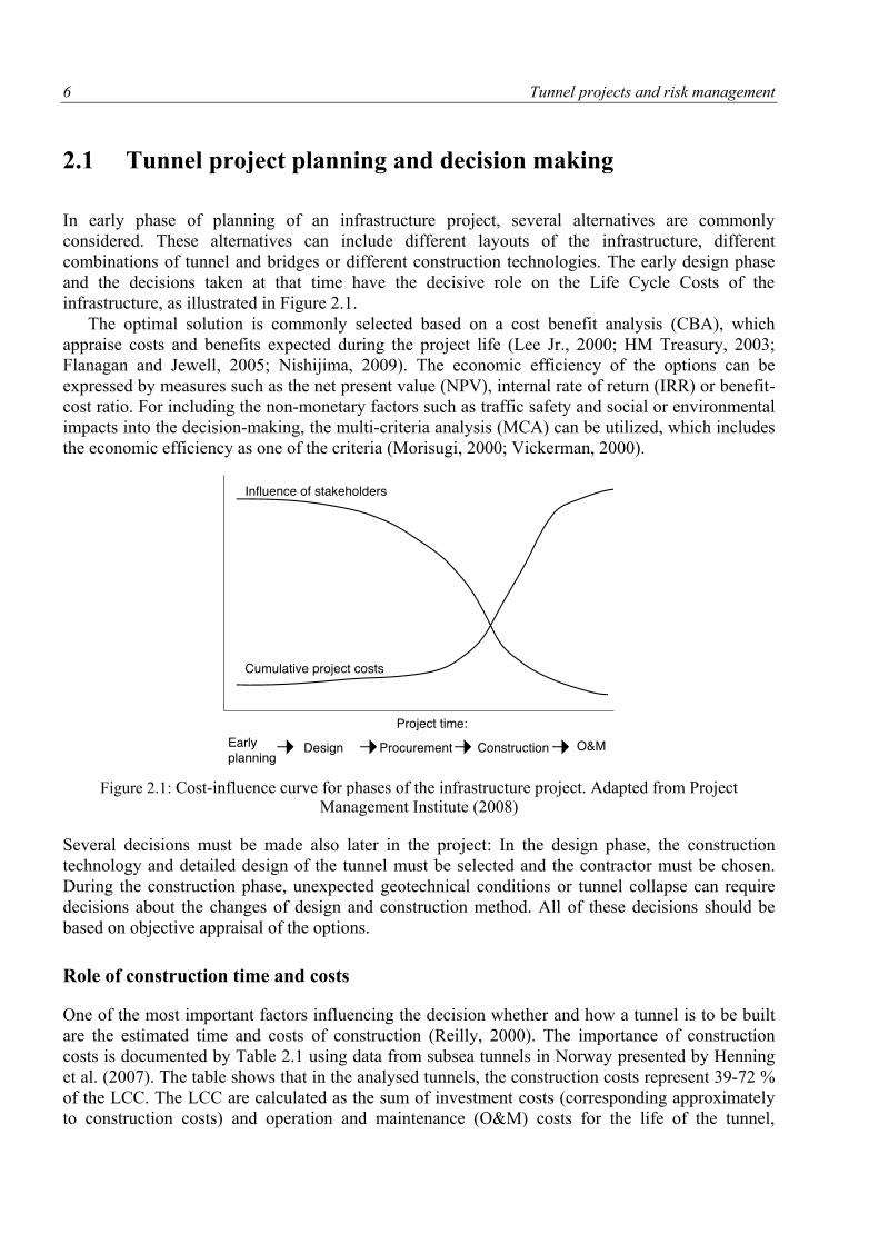
and the decisions taken at that time have the decisive role on the Life Cycle Costs of the
infrastructure, as illustrated in Figure 2.1.
The optimal solution is commonly selected based on a cost benefit analysis (CBA), which
appraise costs and benefits expected during the project life (Lee Jr., 2000; HM Treasury, 2003;
Flanagan and Jewell, 2005; Nishijima, 2009). The economic efficiency of the options can be
expressed by measures such as the net present value (NPV), internal rate of return (IRR) or benefit-
cost ratio. For including the non-monetary factors such as traffic safety and social or environmental
impacts into the decision-making, the multi-criteria analysis (MCA) can be utilized, which includes
the economic efficiency as one of the criteria (Morisugi, 2000; Vickerman, 2000).
Figure 2.1: Cost-influence curve for phases of the infrastructure project. Adapted from Project Management Institute (2008)
Several decisions must be made also later in the project: In the design phase, the construction
technology and detailed design of the tunnel must be selected and the contractor must be chosen.
During the construction phase, unexpected geotechnical conditions or tunnel collapse can require
decisions about the changes of design and construction method. All of these decisions should be
based on objective appraisal of the options.
Role of construction time and costs
One of the most important factors influencing the decision whether and how a tunnel is to be built
are the estimated time and costs of construction (Reilly, 2000). The importance of construction
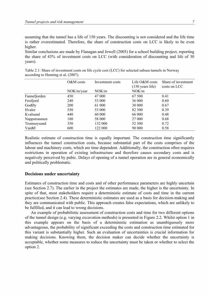
costs is documented by Table 2.1 using data from subsea tunnels in Norway presented by Henning
et al. (2007). The table shows that in the analysed tunnels, the construction costs represent 39-72 %
of the LCC. The LCC are calculated as the sum of investment costs (corresponding approximately
to construction costs) and operation and maintenance (O&M) costs for the life of the tunnel,
Tunnel projects and risk management 7
assuming that the tunnel has a life of 150 years. The discounting is not considered and the life time
is rather overestimated. Therefore, the share of construction costs on LCC is likely to be even
higher.
Similar conclusions are made by Flanagan and Jewell (2005) for a school building project, reporting
the share of 43% of investment costs on LCC (with consideration of discounting and life of 30
years).
Table 2.1: Share of investment costs on life cycle cost (LCC) for selected subsea tunnels in Norway
according to Henning et al. (2007).
O&M costs Investment costs Life O&M costs Share of investment
(150 years life) costs on LCC
NOK/m/year NOK/m NOK/m
Fannefjorden 450 47 000 67 500 0.41
Freifjord 240 53 000 36 000 0.60
GodØy 200 61 000 30 000 0.67
Hvaler 550 53 000 82 500 0.39
Kvalsund 440 60 000 66 000 0.48
Nappstraumen 180 58 000 27 000 0.68
Tromsoysund 350 132 000 52 500 0.72
VardØ 600 122 000 90 000 0.58
Realistic estimate of construction time is equally important. The construction time significantly
influences the tunnel construction costs, because substantial part of the costs comprises of the
labour and machinery costs, which are time dependent. Additionally, the construction often requires
restrictions in operation of existing infrastructure and therefore causes secondary costs and is
negatively perceived by pubic. Delays of opening of a tunnel operation are in general economically
and politically problematic.
Decisions under uncertainty
Estimates of construction time and costs and of other performance parameters are highly uncertain
(see Section 2.7). The earlier in the project the estimates are made, the higher is the uncertainty. In
spite of that, most stakeholders require a deterministic estimate of costs and time in the current
practice(see Section 2.4). These deterministic estimates are used as a basis for decision-making and
they are communicated with public. This approach creates false expectations, which are unlikely to
be fulfilled, and it can lead to wrong decisions.
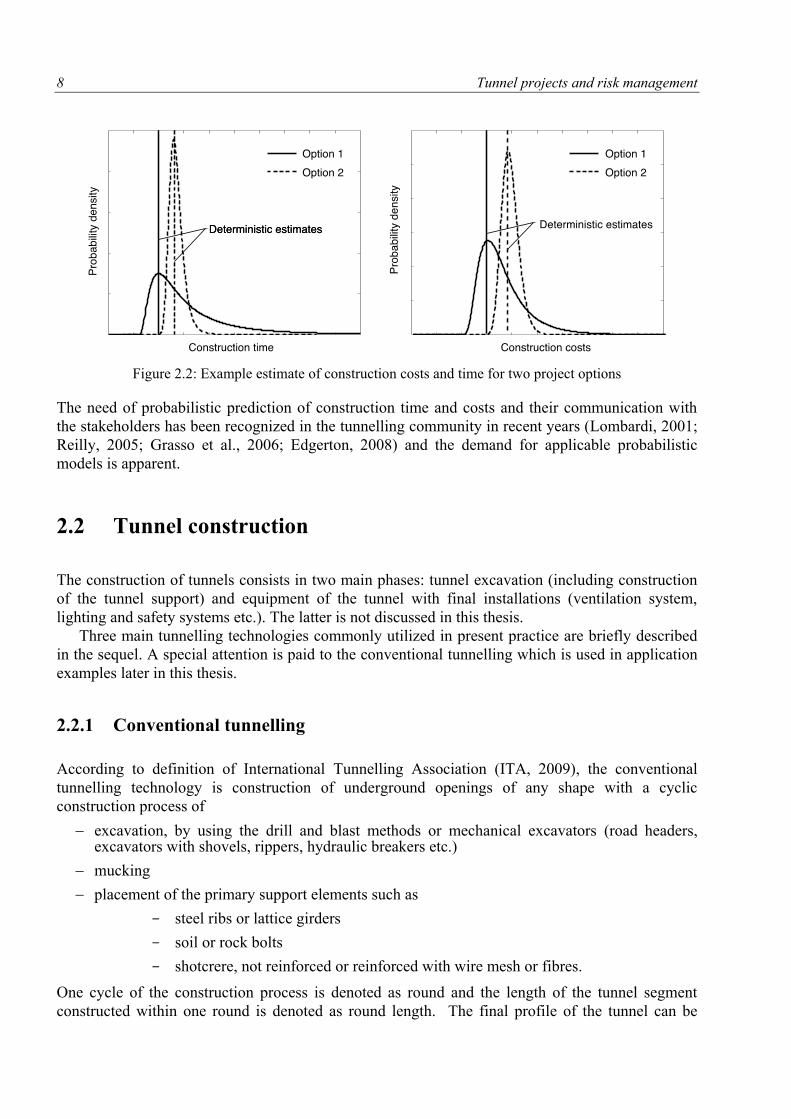
An example of probabilistic assessment of construction costs and time for two different options
of the tunnel design (e.g. varying excavation methods) is presented in Figure 2.2. Whilst option 1 in
this example appears on the basis of a deterministic estimation as unambiguously more
advantageous, the probability of significant exceeding the costs and construction time estimated for
this variant is substantially higher. Such an evaluation of uncertainties is crucial information for
making decisions. Knowing them, the decision maker can decide whether the uncertainty is
acceptable, whether some measures to reduce the uncertainty must be taken or whether to select the
option 2.
8 Tunnel projects and risk management
Figure 2.2: Example estimate of construction costs and time for two project options
The need of probabilistic prediction of construction time and costs and their communication with
the stakeholders has been recognized in the tunnelling community in recent years (Lombardi, 2001;
Reilly, 2005; Grasso et al., 2006; Edgerton, 2008) and the demand for applicable probabilistic
models is apparent.
2.2 Tunnel construction
The construction of tunnels consists in two main phases: tunnel excavation (including construction
of the tunnel support) and equipment of the tunnel with final installations (ventilation system,
lighting and safety systems etc.). The latter is not discussed in this thesis.
Three main tunnelling technologies commonly utilized in present practice are briefly described
in the sequel. A special attention is paid to the conventional tunnelling which is used in application
examples later in this thesis.
2.2.1 Conventional tunnelling
According to definition of International Tunnelling Association (ITA, 2009), the conventional
tunnelling technology is construction of underground openings of any shape with a cyclic
construction process of
excavation, by using the drill and blast methods or mechanical excavators (road headers, excavators with shovels, rippers, hydraulic breakers etc.)
mucking
placement of the primary support elements such as
steel ribs or lattice girders
soil or rock bolts
shotcrere, not reinforced or reinforced with wire mesh or fibres.
One cycle of the construction process is denoted as round and the length of the tunnel segment
constructed within one round is denoted as round length. The final profile of the tunnel can be
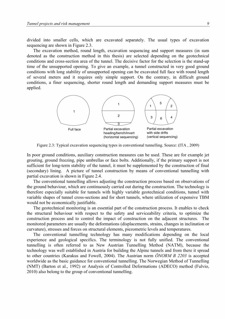
Tunnel projects and risk management 9
divided into smaller cells, which are excavated separately. The usual types of excavation
sequencing are shown in Figure 2.3.
The excavation method, round length, excavation sequencing and support measures (in sum
denoted as the construction method in this thesis) are selected depending on the geotechnical
conditions and cross-section area of the tunnel. The decisive factor for the selection is the stand-up
time of the unsupported opening. To give an example, a tunnel constructed in very good ground
conditions with long stability of unsupported opening can be excavated full face with round length
of several meters and it requires only simple support. On the contrary, in difficult ground
conditions, a finer sequencing, shorter round length and demanding support measures must be
applied.
Figure 2.3: Typical excavation sequencing types in conventional tunnelling. Source: (ITA , 2009)
In poor ground conditions, auxiliary construction measures can be used. These are for example jet
grouting, ground freezing, pipe umbrellas or face bolts. Additionally, if the primary support is not
sufficient for long-term stability of the tunnel, it must be supplemented by the construction of final
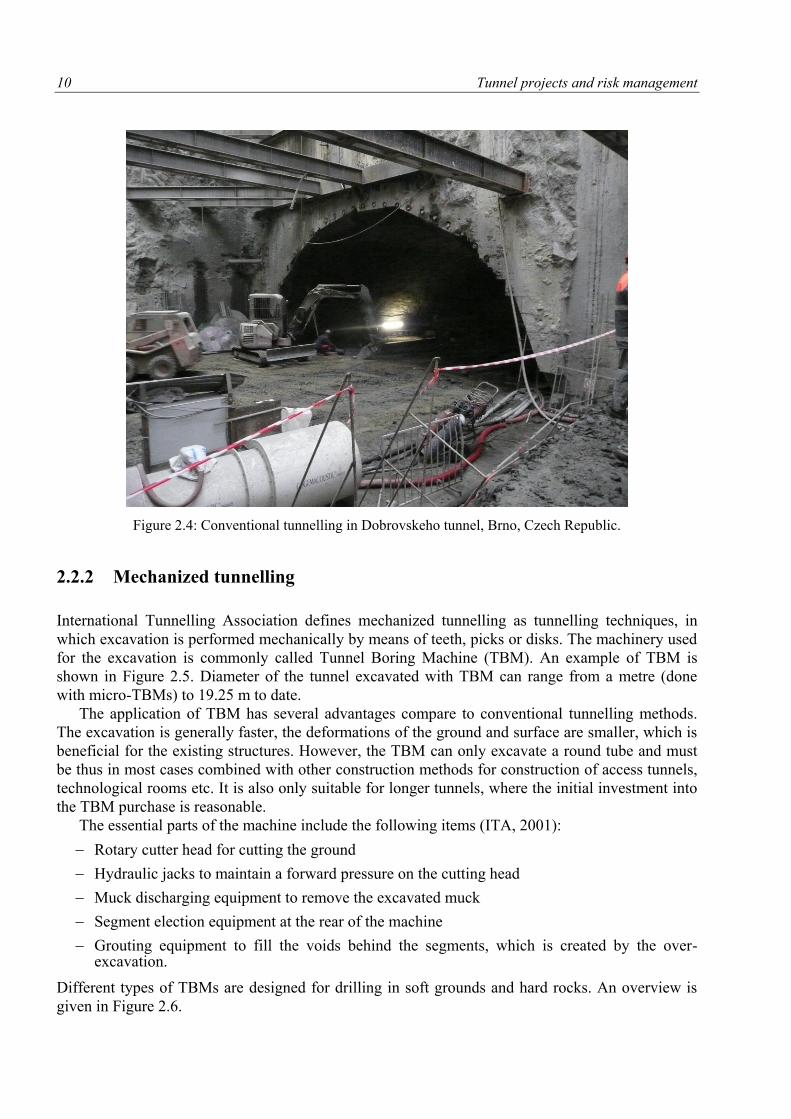
(secondary) lining. A picture of tunnel construction by means of conventional tunnelling with
partial excavation is shown in Figure 2.4.
The conventional tunnelling allows adjusting the construction process based on observations of
the ground behaviour, which are continuously carried out during the construction. The technology is
therefore especially suitable for tunnels with highly variable geotechnical conditions, tunnel with
variable shapes of tunnel cross-sections and for short tunnels, where utilization of expensive TBM
would not be economically justifiable.
The geotechnical monitoring is an essential part of the construction process. It enables to check
the structural behaviour with respect to the safety and serviceability criteria, to optimize the
construction process and to control the impact of construction on the adjacent structures. The
monitored parameters are usually the deformations (displacements, strains, changes in inclination or
curvature), stresses and forces on structural elements, piezometric levels and temperatures.
The conventional tunnelling technology has many modifications depending on the local
experience and geological specifics. The terminology is not fully unified. The conventional
tunnelling is often referred to as New Austrian Tunnelling Method (NATM), because the
technology was well established in Austria for building the Alpine tunnels and from there it spread
to other countries (Karakus and Fowell, 2004). The Austrian norm ÖNORM B 2203 is accepted
worldwide as the basic guidance for conventional tunnelling. The Norwegian Method of Tunnelling
(NMT) (Barton et al., 1992) or Analysis of Controlled Deformations (ADECO) method (Fulvio,
2010) also belong to the group of conventional tunnelling.
10 Tunnel projects and risk management
Figure 2.4: Conventional tunnelling in Dobrovskeho tunnel, Brno, Czech Republic.
2.2.2 Mechanized tunnelling
International Tunnelling Association defines mechanized tunnelling as tunnelling techniques, in
which excavation is performed mechanically by means of teeth, picks or disks. The machinery used
for the excavation is commonly called Tunnel Boring Machine (TBM). An example of TBM is
shown in Figure 2.5. Diameter of the tunnel excavated with TBM can range from a metre (done
with micro-TBMs) to 19.25 m to date.
The application of TBM has several advantages compare to conventional tunnelling methods.
The excavation is generally faster, the deformations of the ground and surface are smaller, which is
beneficial for the existing structures. However, the TBM can only excavate a round tube and must
be thus in most cases combined with other construction methods for construction of access tunnels,
technological rooms etc. It is also only suitable for longer tunnels, where the initial investment into
the TBM purchase is reasonable.
The essential parts of the machine include the following items (ITA, 2001):
Rotary cutter head for cutting the ground
Hydraulic jacks to maintain a forward pressure on the cutting head
Muck discharging equipment to remove the excavated muck
Segment election equipment at the rear of the machine
Grouting equipment to fill the voids behind the segments, which is created by the over-excavation.
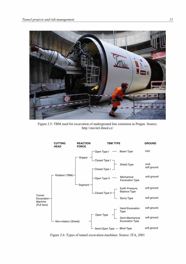
Different types of TBMs are designed for drilling in soft grounds and hard rocks. An overview is
given in Figure 2.6.
Tunnel projects and risk management 11
Figure 2.5: TBM used for excavation of underground line extension in Prague. Source:
http://stavitel.ihned.cz/
Figure 2.6: Types of tunnel excavation machines. Source: ITA, 2001
12 Tunnel projects and risk management
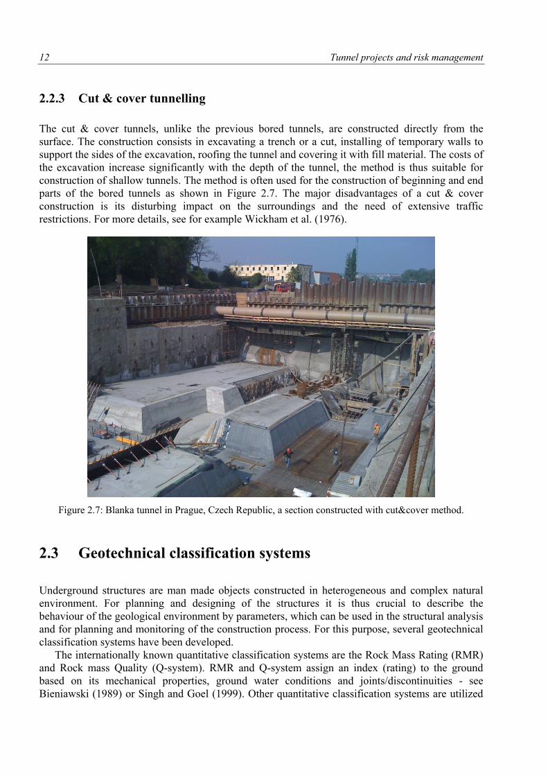
2.2.3 Cut & cover tunnelling
The cut & cover tunnels, unlike the previous bored tunnels, are constructed directly from the
surface. The construction consists in excavating a trench or a cut, installing of temporary walls to
support the sides of the excavation, roofing the tunnel and covering it with fill material. The costs of
the excavation increase significantly with the depth of the tunnel, the method is thus suitable for
construction of shallow tunnels. The method is often used for the construction of beginning and end
parts of the bored tunnels as shown in Figure 2.7. The major disadvantages of a cut & cover
construction is its disturbing impact on the surroundings and the need of extensive traffic
restrictions. For more details, see for example Wickham et al. (1976).
Figure 2.7: Blanka tunnel in Prague, Czech Republic, a section constructed with cut&cover method.
2.3 Geotechnical classification systems
Underground structures are man made objects constructed in heterogeneous and complex natural
environment. For planning and designing of the structures it is thus crucial to describe the
behaviour of the geological environment by parameters, which can be used in the structural analysis
and for planning and monitoring of the construction process. For this purpose, several geotechnical
classification systems have been developed.
The internationally known quantitative classification systems are the Rock Mass Rating (RMR)
and Rock mass Quality (Q-system). RMR and Q-system assign an index (rating) to the ground
based on its mechanical properties, ground water conditions and joints/discontinuities - see
Bieniawski (1989) or Singh and Goel (1999). Other quantitative classification systems are utilized
Tunnel projects and risk management 13
locally in individual countries or areas, for example the Czech method by Tesař (1989) assigning a
so called QTS index. A comparison of this three indexing classification systems is given in Table
2.2.
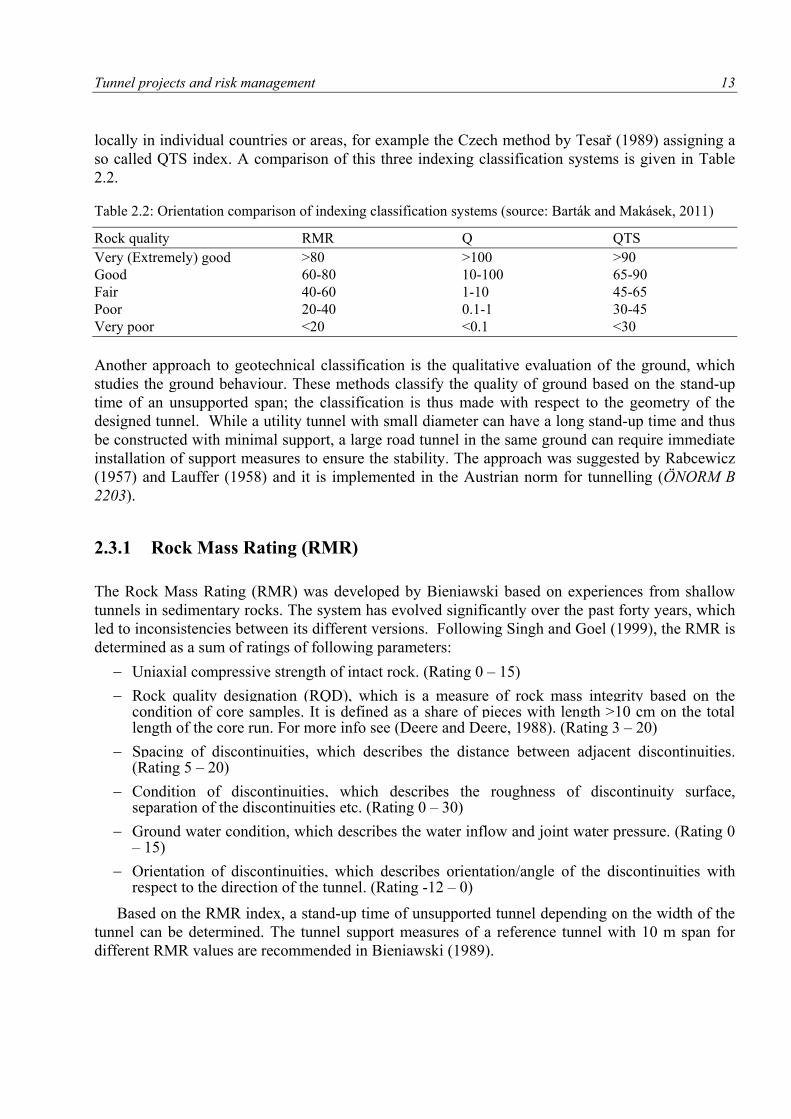
Table 2.2: Orientation comparison of indexing classification systems (source: Barták and Makásek, 2011)
Rock quality RMR Q QTS
Very (Extremely) good >80 >100 >90
Good 60-80 10-100 65-90
Fair 40-60 1-10 45-65
Poor 20-40 0.1-1 30-45
Very poor <20 <0.1 <30
Another approach to geotechnical classification is the qualitative evaluation of the ground, which
studies the ground behaviour. These methods classify the quality of ground based on the stand-up
time of an unsupported span; the classification is thus made with respect to the geometry of the
designed tunnel. While a utility tunnel with small diameter can have a long stand-up time and thus
be constructed with minimal support, a large road tunnel in the same ground can require immediate
installation of support measures to ensure the stability. The approach was suggested by Rabcewicz
(1957) and Lauffer (1958) and it is implemented in the Austrian norm for tunnelling (ÖNORM B
2203).
2.3.1 Rock Mass Rating (RMR)
The Rock Mass Rating (RMR) was developed by Bieniawski based on experiences from shallow
tunnels in sedimentary rocks. The system has evolved significantly over the past forty years, which
led to inconsistencies between its different versions. Following Singh and Goel (1999), the RMR is
determined as a sum of ratings of following parameters:
Uniaxial compressive strength of intact rock. (Rating 0 – 15)
Rock quality designation (RQD), which is a measure of rock mass integrity based on the condition of core samples. It is defined as a share of pieces with length >10 cm on the total length of the core run. For more info see (Deere and Deere, 1988). (Rating 3 – 20)
Spacing of discontinuities, which describes the distance between adjacent discontinuities. (Rating 5 – 20)
Condition of discontinuities, which describes the roughness of discontinuity surface, separation of the discontinuities etc. (Rating 0 – 30)
Ground water condition, which describes the water inflow and joint water pressure. (Rating 0 – 15)
Orientation of discontinuities, which describes orientation/angle of the discontinuities with respect to the direction of the tunnel. (Rating -12 – 0)
Based on the RMR index, a stand-up time of unsupported tunnel depending on the width of the
tunnel can be determined. The tunnel support measures of a reference tunnel with 10 m span for
different RMR values are recommended in Bieniawski (1989).
14 Tunnel projects and risk management
2.3.2 Q-system
The Q-system was proposed at The Norwegian Geotechnical Institute. The Q value is determined as
(Singh and Goel, 1999):
, (2.1)
where is the Rock quality designation index (Deere and Deere, 1988); is the joint set
number representing the number of joint sets (sets of parallel joints); is the joint roughness
number for critically oriented joint sets; is the joint alteration number for critically oriented joint
sets; is the joint water reduction factor and SRF is the stress reduction factor.
Based on the Q value and the tunnel dimensions, the appropriate support patterns are
recommended in the literature (Barton et al., 1974).
2.3.3 Czech classification - QTS index
The QTS index classification was proposed based on experiences from construction of the Prague
underground system (Tesař, 1989). The index is calculated as:
(2.2)
where is the compressive strength of the rock, is the average distance of discontinuities and
is the depth of the investigated layer. and are reduction coefficients depending on the type
and orientation of discontinuities and on water conditions.
2.3.4 Qualitative and project specific classification systems
The qualitative classifications following the ÖNORM B 2203 classify the ground based on its
behaviour as follows:
The decisive parameters influencing the ground behaviour are selected depending on the type of geology. Other parameters are important in rocks, other in soils. For example, in volcanic rocks, the lithology, strength and types of discontinuities are the most important parameters.
Based on evaluation of the geotechnical parameters, hydrological conditions and geometry of the tunnel (cross-section area, position), the different types of ground behaviour such as ravelling, squeezing, swelling or slaking are predicted and the stability of the opening is assessed. The ground is classified into classes, which are characterized by the stand-up time of unsupported opening.
In the design and construction of a tunnel, different classification methods are commonly combined
and a project specific classification system is defined. This system considers the specifics of the
local geology, the parameters of the tunnel (geometry, inclination) and the construction technology
(conventional vs. mechanized tunnelling). The project specific classification system defines
commonly 3-10 ground classes, which are used to design the tunnel support and to select the
construction method (e.g. round length in case of conventional tunnelling, mode of the TBM in case
of the mechanized tunnelling). Importantly, the ground classes also serve as the basis for pricing
Tunnel projects and risk management 15
and scheduling of the construction works. In some types of contract, the payments for construction
works are determined based on the observed ground classes.
2.3.5 Comparison of the classification systems
As is evident from previous sub-sections, the approaches to geotechnical classification differ
significantly and a clear relation between the systems cannot be found. The relation between
quantitative/indexing methods such as RMR or Q-system cannot be defined unambiguously,
because the systems consider different criteria (Goel et al., 1996; Laderian and Abaspoor, 2012).
Additionally, the evaluated parameters are not exactly measurable, their assessment depends on
“fuzzy” expert judgement (Aydin, 2004) and the final classification is thus also influenced by the
expert.
The qualitative approaches are site specific from their definition, because they take into account
the characteristics of the tunnel to be built and the construction method. The many modifications of
existing classification systems show that utilization of an universally valid system is not realistic.
The only factor, which can be used as the integrating parameter of presented geotechnical
classification systems and which can serve for their comparison, is the stand-up time of an
unsupported opening (Barták and Makásek, 2011).
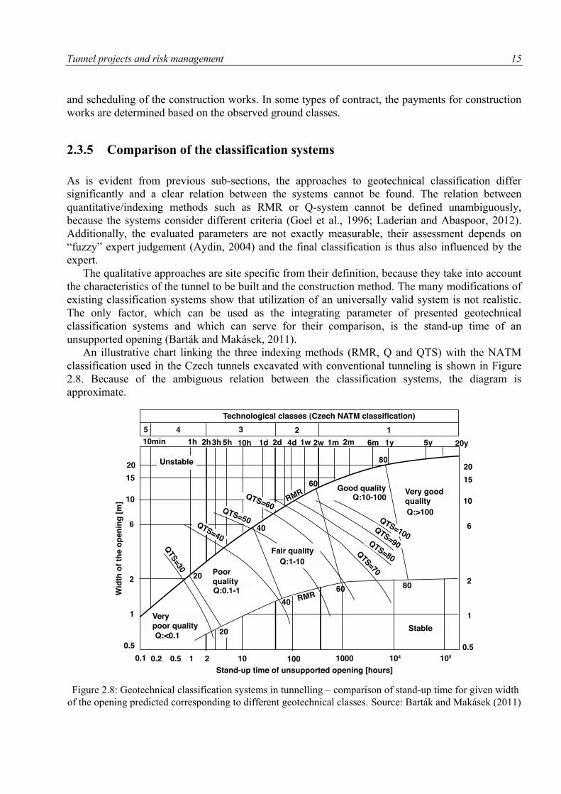
An illustrative chart linking the three indexing methods (RMR, Q and QTS) with the NATM
classification used in the Czech tunnels excavated with conventional tunneling is shown in Figure
2.8. Because of the ambiguous relation between the classification systems, the diagram is
approximate.
Figure 2.8: Geotechnical classification systems in tunnelling – comparison of stand-up time for given width
of the opening predicted corresponding to different geotechnical classes. Source: Barták and Makásek (2011)
16 Tunnel projects and risk management
2.4 Estimation of construction time and costs
Estimates of tunnel construction time and costs are a fundamental part of the tunnel project
planning. The time and costs of tunnel construction depend primarily on the following factors:
Geological conditions (e.g. mechanical properties of the ground, frequency and orientation of discontinuities)
Hydrological conditions
Frequency of changes of the geological and hydrological conditions - (in)homogeneity of the environment
Cross-section area of the tunnel
Length of the tunnel
Inclination of the tunnel
Depth of the tunnel/height of overburden
Affected structures and systems (requirements on maximal deformations, protection of water systems and environment, operational constraints)
Quality of planning and design
Construction management and control, quality of construction works
The methods of time and costs estimates vary in different project phases. In the early design phase,
only little information is available about the geotechnical conditions, tunnel design and construction
technology. Therefore, only rough estimates using the experience and/or data from tunnels
constructed in the past can be provided. Analyses of tunnel construction time and costs are
available in the literature: Burbaum et al. (2005) provides a detailed guidance for tunnel
construction costs estimates in early design phases, which is based on the experiences in Hessen,
Germany. Kim and Bruland (2009) study the dependence of tunnel construction time on the
geotechnical conditions classified using the Q-system (Section 2.3.2) and the cross-section area of
the tunnel. Zare (2007) and Zare and Bruland (2007) analyse the construction time and costs in
conventional tunnels. These three studies are based on Norwegian experiences and a detailed
simulation of the construction process. Farrokh et al. (2012) presents a number of models for the
prediction of the TBM penetration rate and compares the estimates of these models with data from
tunnels constructed in the past. Other approach for tunnel construction time estimate in dependence
on the geology, excavation technology, support system and other factors is presented in Singh and
Goel (1999).
In later planning phases, geotechnical surveys are carried out and a detailed tunnel design is
prepared. Based on this information, more precise time and costs estimates are made taking into
account the particular activities of the construction process and the associated utilization of
resources such as material, labour and machinery. The estimates are done by experience cost
estimators and projects planners. The estimators can use several simulation tools for modelling of
the construction processes, an overview of the tools is given for example in Jimenez (1999).
Applications of simulation models for tunnelling are presented in AbouRizk et al. (1999) and (Zhou
et al., 2008). Some of the models allow to take into account uncertainties of the estimates, as will be
discussed later in the Section 3.2. It should be noted that construction of tunnels is a chain of
repetitive activities whose order is strictly given. There is therefore negligible uncertainty in the
determination of critical path, which is the longest path through a network of construction activities
Tunnel projects and risk management 17
with respect to the given order of activities. From the modelling point of view, this is a big
advantage compared to non-linear types of structures (Ökmen and Öztaş, 2008).
In practice, the construction costs and time are often underestimated: (Flyvbjerg et al., 2002)
show that final construction costs of tunnel and bridge construction projects are, on average, 34%
above original estimates made at the time of decision to build. The study further shows that there
has been no improvement over the past seventy years. The reasons for this systematic
underestimation are discussed in Flyvbjerg, (2006): First, people tend to “judge future events in a
more positive light than is warranted by actual experience”; this psychological phenomena is called
optimism bias. Second, the system of administering and financing of transport projects often
motivates the people interested in realization of the project to purposely underestimate the
construction costs and time, because it improves the chance of the project to be financed; this
political and organizational phenomenon is denoted as strategic misrepresentation.
Based on results of these studies, the British authorities recommend adjusting the cost estimates
for bias and risk (HM Treasury, 2003). This adjustment should be based on analysis of projects
constructed in the past. Extensive statistical analyses of the construction cost increase were made
(Flyvbjerg and COWI, 2004; Flyvbjerg, 2006). These allowed determining the uplifts of the
deterministic estimate for different reference project classes. For example, to obtain a cost estimate
of tunnel or bridge construction projects with 80% probability of not being exceeded, the
deterministic expert estimate should be increased by 55%. These studies are the first attempts
known to the author, which aim at quantifying the uncertainty in cost estimates based on analysis of
data from previous projects. The utilized approach differs from the one presented later in Chapter 7
of this thesis in two main points: First, the authors do not study the actual cost related to a unit
length (or unit volume) of the infrastructure but they examine the probability distribution of cost
overrun. This approach seems to be unlucky. Assuming that the method will be systematically used
in the practice and the practitioners will become more aware of the uncertainties in the estimates,
they might start estimating even the deterministic costs more realistically. In such a case, the
present study of the cost overruns will not be valid anymore. Second, the specifics of individual
projects (e.g. geology, geometry and layout of the infrastructure, location in a country and
inside/outside of a city) are not considered in the analysis. The practitioners will hardly accept the
rough categorization of the projects and neglecting the local specifics. The guidance therefore
allows a significant space for expert judgement and the benefits of the statistical approach are thus
significantly reduced.
2.5 Tunnel construction failures
Tunnel construction failures are extraordinary events, which have severe impact on the construction
process. They may cause high financial losses, severe delays or even human injuries or death
(IMIA, 2006). The control of tunnel failures risks is thus of crucial importance.
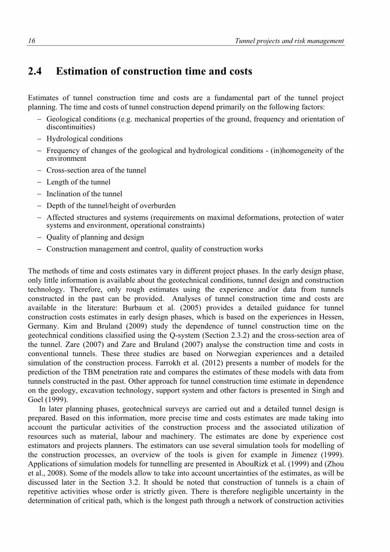
The most frequently reported tunnel construction failures are the cave-in collapses, tunnel
flooding, portal instability or excessive deformation of the tunnel tube and the overburden. The
tunnel construction failures can cause damages on adjacent buildings and infrastructure and they are
thus especially adverse in tunnels built in the cities. Examples of cave-in collapses from the Czech
Republic are shown in Figure 2.9.
18 Tunnel projects and risk management
Figure 2.9: Examples of a cave-in collapses, which occured during construction of tunnels in the Czech
Republic: (a) Jablunkov railway tunnel, (b) Blanka road tunnel. Source: www.idnes.cz.
Efforts to learn a lesson from past errors led to the development of numerous databases of tunnel
construction failures. The British study HSE (2006) offers a database of over a hundred collapses; it
is an expansion of the data contained in the preceding publication (HSE, 1996). The study analyses
the most frequent causes and consequences of the collapses, focusing on tunnels driven in urban
areas, through soils and lower quality rocks.
An analysis of causes and failure mechanisms is provided by the diploma thesis of Seidenfuss
(2006). The database contains over one hundred and ten cases of tunnel excavation failures. The
work analyses above all the causes of the collapses and measures taken after their occurrence. The
cases partially overlap with the database of thirty-three failures which was developed within the
framework of Master thesis by Stallmann (2005).
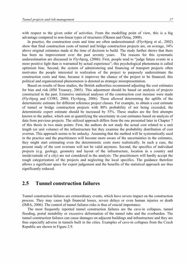
To date, the most extensive database of approximately two hundred tunnel construction failures
was compiled within dissertation by Sousa (2010). The data were collected from the public domain
and from correspondence with experts. The database summarizes information on the tunnels and on
development and consequences of the failures. So far, the database is unfortunately not accessible
online. The geographical distribution of the collected tunnel failures and the distribution of the
types of involved tunnels are shown in Figure 2.10.
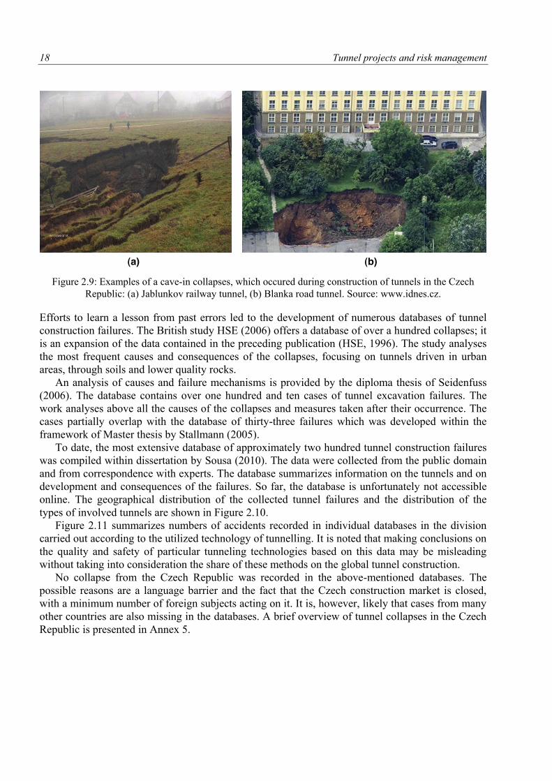
Figure 2.11 summarizes numbers of accidents recorded in individual databases in the division
carried out according to the utilized technology of tunnelling. It is noted that making conclusions on
the quality and safety of particular tunneling technologies based on this data may be misleading
without taking into consideration the share of these methods on the global tunnel construction.
No collapse from the Czech Republic was recorded in the above-mentioned databases. The
possible reasons are a language barrier and the fact that the Czech construction market is closed,
with a minimum number of foreign subjects acting on it. It is, however, likely that cases from many
other countries are also missing in the databases. A brief overview of tunnel collapses in the Czech
Republic is presented in Annex 5.
Tunnel projects and risk management 19
Figure 2.10: Database of tunnel failures collected by Sousa (2010): (a) number of collapses collected in
different continents, (b) share of the tunnel types in the database.
Figure 2.11: Numbers of accidents compiled in the four databases in the division according to the tunnelling
technology (* mechanized excavation includes all cases, where “non_NATM” is referred to without any
more detailed description)
2.6 Risk management
Risk management is an integral part of majority of infrastructure projects. Many methodologies and
guidance have been developed. This section gives a brief overview of the methodologies and their
applicability.
Section 2.6.1 describes a general concept of risk management recommended by ISO 31000:2009
guidelines on risk (ISO, 2009). The thesis also takes over the definition of risk introduced by this
document. The risk is thus defined as:
“effect of uncertainty on objectives”.
Section 2.6.2 concerns with risk management of construction projects and of tunnels in
particular. In Sections 2.6.3 and 2.6.4, the role of risk in procurement and insurance of the tunnel
projects is discussed.
20 Tunnel projects and risk management
2.6.1 Risk management process
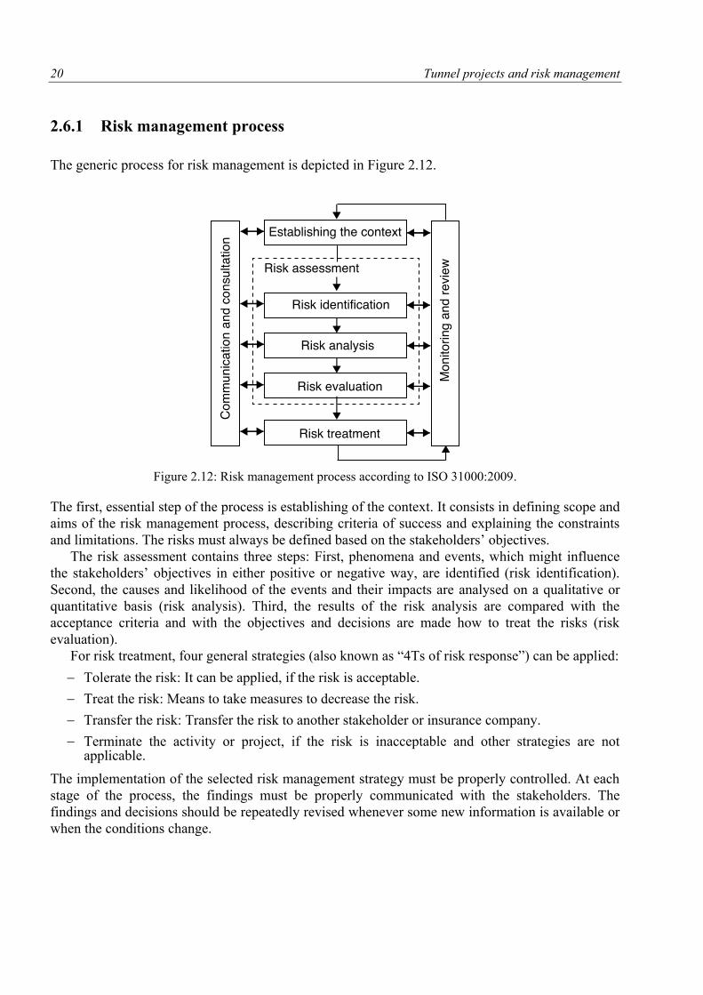
The generic process for risk management is depicted in Figure 2.12.
Figure 2.12: Risk management process according to ISO 31000:2009.
The first, essential step of the process is establishing of the context. It consists in defining scope and
aims of the risk management process, describing criteria of success and explaining the constraints
and limitations. The risks must always be defined based on the stakeholders’ objectives.
The risk assessment contains three steps: First, phenomena and events, which might influence
the stakeholders’ objectives in either positive or negative way, are identified (risk identification).
Second, the causes and likelihood of the events and their impacts are analysed on a qualitative or
quantitative basis (risk analysis). Third, the results of the risk analysis are compared with the
acceptance criteria and with the objectives and decisions are made how to treat the risks (risk
evaluation).
For risk treatment, four general strategies (also known as “4Ts of risk response”) can be applied:
Tolerate the risk: It can be applied, if the risk is acceptable.
Treat the risk: Means to take measures to decrease the risk.
Transfer the risk: Transfer the risk to another stakeholder or insurance company.
Terminate the activity or project, if the risk is inacceptable and other strategies are not applicable.
The implementation of the selected risk management strategy must be properly controlled. At each
stage of the process, the findings must be properly communicated with the stakeholders. The
findings and decisions should be repeatedly revised whenever some new information is available or
when the conditions change.
Tunnel projects and risk management 21
2.6.2 Risk management of construction projects
Application of risk management in construction industry has been motivated by increasing
complexity of the construction projects and by pressure for cost savings and for construction time
reduction. Identification of risks in early design phase allows significant reduction of life-cycle
costs through improvements of the design and planning and through appropriate treatment of the
risk in the later phases. Generic guidance for the risk management process in construction projects
can be found for example in Flanagan and Norman (1993), Edwards (1995), Wang and Roush
(2000), Revere (2003), Institution of Civil Engineers et al. (2005), Smith et al. (2006) and Rozsypal
(2008). A risk management section is also included in the broadly used manual of project
management (Project Management Institute, 2008).
Some manuals have been developed specifically for the underground construction and
tunnelling projects (Clayton, 2001; Eskesen et al., 2004; Staveren, 2006). In these manuals, a
special attention is paid to the geotechnical risks, which play a crucial role in the underground
construction.
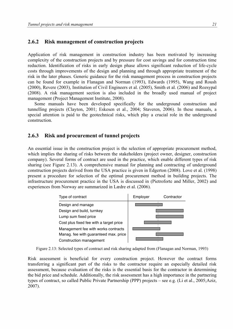
2.6.3 Risk and procurement of tunnel projects
An essential issue in the construction project is the selection of appropriate procurement method,
which implies the sharing of risks between the stakeholders (project owner, designer, construction
company). Several forms of contract are used in the practice, which enable different types of risk
sharing (see Figure 2.13). A comprehensive manual for planning and contracting of underground
construction projects derived from the USA practice is given in Edgerton (2008). Love et al. (1998)
present a procedure for selection of the optimal procurement method in building projects. The
infrastructure procurement practice in the USA is discussed in (Pietroforte and Miller, 2002) and
experiences from Norway are summarized in Lædre et al. (2006).
Figure 2.13: Selected types of contract and risk sharing adapted from (Flanagan and Norman, 1993)
Risk assessment is beneficial for every construction project. However the contract forms
transferring a significant part of the risks to the contractor require an especially detailed risk
assessment, because evaluation of the risks is the essential basis for the contractor in determining
the bid price and schedule. Additionally, the risk assessment has a high importance in the partnering
types of contract, so called Public Private Partnership (PPP) projects – see e.g. (Li et al., 2005;Aziz,
2007).
22 Tunnel projects and risk management
2.6.4 Risk and insurance of tunnel projects
Insuring of construction projects is a common practice in countries such as USA or Great Britain.
The insurers offer project specific insurance covering for example claims for injury, third party
property damage or damage to the constructed structure, material and machinery. Standard types of
insurance schemes for construction projects are the Contractors All Risk (CAR) insurance or
Construction Project All risk Insurance (Allianz Insurence, n.d.). Because the private financing of
the tunnel project has increased in recent years, demand for new types of insurance schemes is
growing: for example Anticipated Loss of Profit / Delay in Start Up (ALOP/DSU) insurance
(Landrin et al., 2006).
After the insurance companies experienced major losses on insured underground project, they
developed codes for tunnel project risk management (ABI and BTS, 2003; ITIG, 2006).
Compliance with the codes is now required from most of the insured projects. Even if the codes are
successfully applied in the practice (Spencer, 2008), insuring of tunnel projects is still very risky
and the insurers must search for methods to improve the assessment of construction project risks.
2.7 Uncertainties in the tunnel projects
All phases of the tunnel project are influenced by numerous uncertainties. These can be categorized
into two groups:
Usual uncertainties in the course of tunnel design, construction and operation
Occurrence of extraordinary events (failures) causing significant unplanned changes of the expected project development
Both types of uncertainties influence the stakeholders’ objectives, which can be expressed using
performance parameters such as costs, time, quality etc. Examples of the uncertainties and
performance parameters, in division to the project phases, are given in Table 2.3.
Table 2.3: Examples of uncertainties and the influenced performance parameters in the tunnel projects
Planning phase Construction phase Operation phase
Usual uncertainties Usual uncertainties Usual uncertainties
- quality of planning team - geological + hydrological cond. - number of vehicles
- quality of designer - performance of the technology - quality of maintenance
- geotechnical survey - quality of organization and works - durability of materials
- tendering - prices of materials, labour…
Extraordinary events Extraordinary events Extraordinary events
- Strong public aversion - Tunnel collapse or flooding - Fire
- Rejection of financing - Unpredicted existing structures - Vehicle accident
- Legislative obstructions - Extensive deformations - Tunnel collapse
Performance parameters Performance parameters Performance parameters
- Land acquisition time and costs - Construction costs - Income/availability
- Design cost, time and quality - Construction time - M&O costs
- Time for acquisition of regulatory - Quality - Environmental impacts
approvals and permits - Financing - Life time
Tunnel projects and risk management 23
Distinguishing between the two types of uncertainties is necessary, because the principal divergence
of their nature requires different approaches to their analysis. It is further evident that the usual
uncertainties influence the occurrence of extraordinary events. For example, unpredicted geological
conditions and poor quality of construction management is likely to lead to a tunnel collapse. These
dependences must therefore be considered in the quantitative risk analysis.
For the modelling purposes it is further convenient to distinguish between the aleatory and
epistemic uncertainties:
Aleatory uncertainty is the natural, intrinsic randomness in the analysed system, which cannot be reduced.
The epistemic uncertainty is the uncertainty resulting from incomplete knowledge of the system and it can be reduced when additional information is available.
To give examples, the geotechnical parameters (e.g. number and orientation of discontinuities,
compressive strength) can include both types of uncertainties. The aleatory uncertainty corresponds
to the spatial randomness of these parameters (the discontinuities are not equally distributed in
space). The epistemic uncertainty results from the fact that we are not able to describe the
randomness with certainty because we only have limited knowledge about the geology (e.g. from
local boreholes). A thorough discussion on aleatory and epistemic uncertainty is available in Der
Kiureghian and Ditlevsen (2009). The authors claim that, in principle, distinguishing between the
two types of uncertainties depends on the view and intentions of the modeller, i.e. on the judgment,
whether or not the uncertainty can be reduced in later phases of the analysis.
2.8 Summary
Chapter 2 introduces the reader into the topic of tunnel project planning and management. While the
remaining part of the thesis only deals with modelling of tunnel construction, Sections 2.1, 2.6 and
2.7 put the construction phase into the context of project’s life cycle. It is shown that the time and
costs of construction are not the only criteria for making decisions, but certainly very important
ones. Additionally, it is demonstrated that analysing the uncertainties and risk is crucial for
identifying optimal solutions in all phases of the project. A categorization of uncertainties
influencing the tunnel projects is brought in this chapter as well, since it is important for their
proper analysis and modelling.
Sections 2.2 - 2.5 briefly discuss the tunnel construction itself. The commonly used tunnelling
technologies are introduced in Section 2.2 with particular attention to the conventional tunnelling,
which is used in application examples later in this thesis. Because the geological conditions and
their proper description is essential for the tunnel construction and for the prediction of the
construction time and costs, Section 2.3 gives a summary of the widely used geotechnical
classification systems. It shows that the description of geotechnical conditions is highly site-
specific. Therefore, the transfer of experiences between different projects is not a straightforward
task and it cannot be easily automated. This issue will be discussed later in relation to the data
analysis in Chapter 7. Section 2.4 briefly explains, how the construction time and costs are
estimated in different phases of the project. At present, the deterministic estimates are used in the
majority of cases. However, the tunnelling community recently recognised the limitations of the
deterministic approach and more attempts are made to quantify the uncertainties and risks (see
Section 3.2). Finally, Section 2.5 discusses the possibility of occurrence of extraordinary events
(failures) during the tunnel construction. These events represent a high risk for the tunnelling

24 Tunnel projects and risk management
procedure, as is shown in several studies collecting information on past events. Modelling of these
events and their impact is discussed also in remaining part of the thesis.
25
Approaches and methods for risk analysis are presented in this chapter. As was introduced in
Section 2.6, the risk is defined as “effect of uncertainty on the objectives”. The uncertainties
influencing the tunnel project were briefly discussed in Section 2.7; it is distinguished between the
usual uncertainties and extraordinary events. The objectives of a tunnel construction (measurable
performance parameters) are as follows:
Completion of the construction on time
Completion of the construction within the budget
Fulfilment of the technical requirements
Ensuring safety during the construction
Minimization of impact on operation of adjacent structures
Minimization of damage to third party property
Avoidance of negative reaction of media and public
In the following, the text mostly focuses on effect of uncertainty on the construction time, partly
also on the construction costs, the other performance parameters are not explicitly considered in this
thesis.
Note that the risk is not a universal quantity. The objectives of individual stakeholders can differ
and they also develop during the project. Additionally, the perception of the consequences of not
meeting the objectives is also individual. Therefore, the risk must always be analysed with regard to
the context and objectives.
The state-of-the-art of tunnel construction risk analysis is summarized in this chapter: Section
3.1 is focused on the qualitative method; Section 3.2 provides an overview of approaches to
quantitative risk analysis. The purpose and limitations of the qualitative and quantitative approaches
are discussed. Section 3.3 introduces selected methods and models for analysis of uncertainty and
risk, which are utilized later in this thesis.
3 Analysis of tunnel construction risk
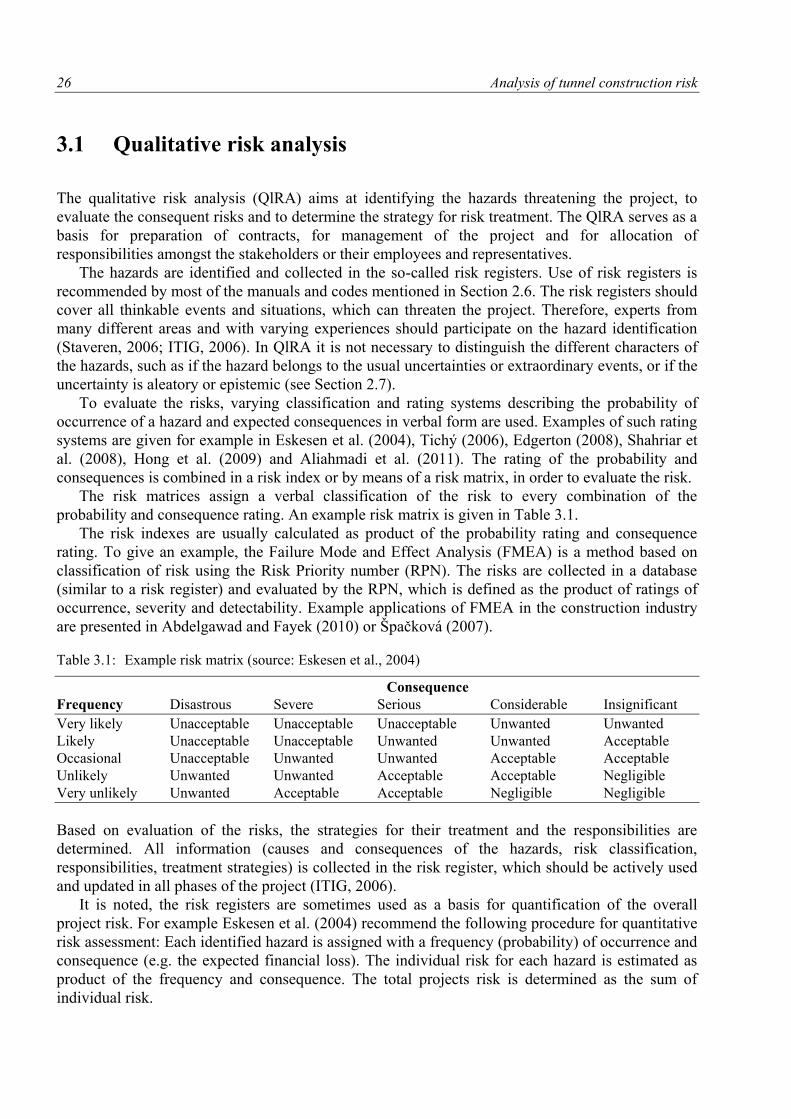
26 Analysis of tunnel construction risk
3.1 Qualitative risk analysis
The qualitative risk analysis (QlRA) aims at identifying the hazards threatening the project, to
evaluate the consequent risks and to determine the strategy for risk treatment. The QlRA serves as a
basis for preparation of contracts, for management of the project and for allocation of
responsibilities amongst the stakeholders or their employees and representatives.
The hazards are identified and collected in the so-called risk registers. Use of risk registers is
recommended by most of the manuals and codes mentioned in Section 2.6. The risk registers should
cover all thinkable events and situations, which can threaten the project. Therefore, experts from
many different areas and with varying experiences should participate on the hazard identification
(Staveren, 2006; ITIG, 2006). In QlRA it is not necessary to distinguish the different characters of
the hazards, such as if the hazard belongs to the usual uncertainties or extraordinary events, or if the
uncertainty is aleatory or epistemic (see Section 2.7).
To evaluate the risks, varying classification and rating systems describing the probability of
occurrence of a hazard and expected consequences in verbal form are used. Examples of such rating
systems are given for example in Eskesen et al. (2004), Tichý (2006), Edgerton (2008), Shahriar et
al. (2008), Hong et al. (2009) and Aliahmadi et al. (2011). The rating of the probability and
consequences is combined in a risk index or by means of a risk matrix, in order to evaluate the risk.
The risk matrices assign a verbal classification of the risk to every combination of the
probability and consequence rating. An example risk matrix is given in Table 3.1.
The risk indexes are usually calculated as product of the probability rating and consequence
rating. To give an example, the Failure Mode and Effect Analysis (FMEA) is a method based on
classification of risk using the Risk Priority number (RPN). The risks are collected in a database
(similar to a risk register) and evaluated by the RPN, which is defined as the product of ratings of
occurrence, severity and detectability. Example applications of FMEA in the construction industry
are presented in Abdelgawad and Fayek (2010) or Špačková (2007).
Table 3.1: Example risk matrix (source: Eskesen et al., 2004)
Consequence
Frequency Disastrous Severe Serious Considerable Insignificant
Very likely Unacceptable Unacceptable Unacceptable Unwanted Unwanted
Likely Unacceptable Unacceptable Unwanted Unwanted Acceptable
Occasional Unacceptable Unwanted Unwanted Acceptable Acceptable
Unlikely Unwanted Unwanted Acceptable Acceptable Negligible
Very unlikely Unwanted Acceptable Acceptable Negligible Negligible
Based on evaluation of the risks, the strategies for their treatment and the responsibilities are
determined. All information (causes and consequences of the hazards, risk classification,
responsibilities, treatment strategies) is collected in the risk register, which should be actively used
and updated in all phases of the project (ITIG, 2006).
It is noted, the risk registers are sometimes used as a basis for quantification of the overall
project risk. For example Eskesen et al. (2004) recommend the following procedure for quantitative
risk assessment: Each identified hazard is assigned with a frequency (probability) of occurrence and
consequence (e.g. the expected financial loss). The individual risk for each hazard is estimated as
product of the frequency and consequence. The total projects risk is determined as the sum of
individual risk.
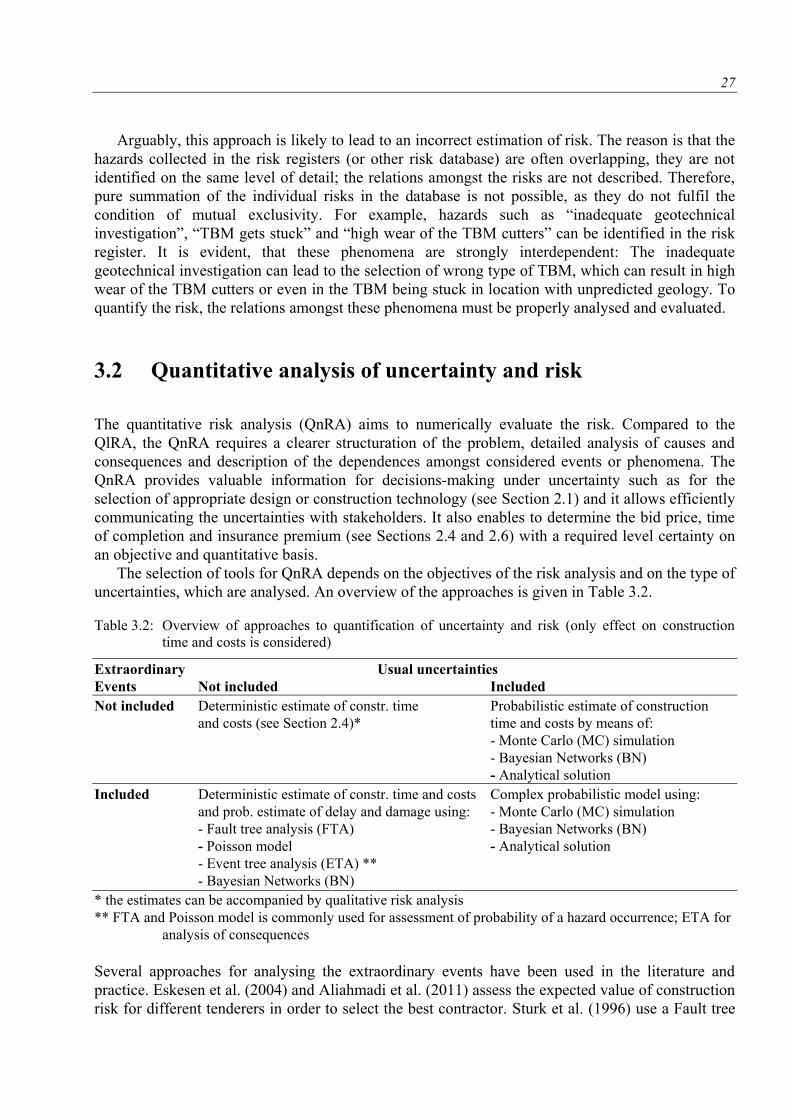
27
Arguably, this approach is likely to lead to an incorrect estimation of risk. The reason is that the
hazards collected in the risk registers (or other risk database) are often overlapping, they are not
identified on the same level of detail; the relations amongst the risks are not described. Therefore,
pure summation of the individual risks in the database is not possible, as they do not fulfil the
condition of mutual exclusivity. For example, hazards such as “inadequate geotechnical
investigation”, “TBM gets stuck” and “high wear of the TBM cutters” can be identified in the risk
register. It is evident, that these phenomena are strongly interdependent: The inadequate
geotechnical investigation can lead to the selection of wrong type of TBM, which can result in high
wear of the TBM cutters or even in the TBM being stuck in location with unpredicted geology. To
quantify the risk, the relations amongst these phenomena must be properly analysed and evaluated.
3.2 Quantitative analysis of uncertainty and risk
The quantitative risk analysis (QnRA) aims to numerically evaluate the risk. Compared to the
QlRA, the QnRA requires a clearer structuration of the problem, detailed analysis of causes and
consequences and description of the dependences amongst considered events or phenomena. The
QnRA provides valuable information for decisions-making under uncertainty such as for the
selection of appropriate design or construction technology (see Section 2.1) and it allows efficiently
communicating the uncertainties with stakeholders. It also enables to determine the bid price, time
of completion and insurance premium (see Sections 2.4 and 2.6) with a required level certainty on
an objective and quantitative basis.
The selection of tools for QnRA depends on the objectives of the risk analysis and on the type of
uncertainties, which are analysed. An overview of the approaches is given in Table 3.2.
Table 3.2: Overview of approaches to quantification of uncertainty and risk (only effect on construction
time and costs is considered)
Extraordinary Usual uncertainties
Events Not included Included
Not included Deterministic estimate of constr. time Probabilistic estimate of construction
and costs (see Section 2.4)* time and costs by means of:
- Monte Carlo (MC) simulation
- Bayesian Networks (BN)
- Analytical solution
Included Deterministic estimate of constr. time and costs Complex probabilistic model using:
and prob. estimate of delay and damage using: - Monte Carlo (MC) simulation
- Fault tree analysis (FTA) - Bayesian Networks (BN)
- Poisson model - Analytical solution
- Event tree analysis (ETA) **
- Bayesian Networks (BN)
* the estimates can be accompanied by qualitative risk analysis
** FTA and Poisson model is commonly used for assessment of probability of a hazard occurrence; ETA for
analysis of consequences
Several approaches for analysing the extraordinary events have been used in the literature and
practice. Eskesen et al. (2004) and Aliahmadi et al. (2011) assess the expected value of construction
risk for different tenderers in order to select the best contractor. Sturk et al. (1996) use a Fault tree
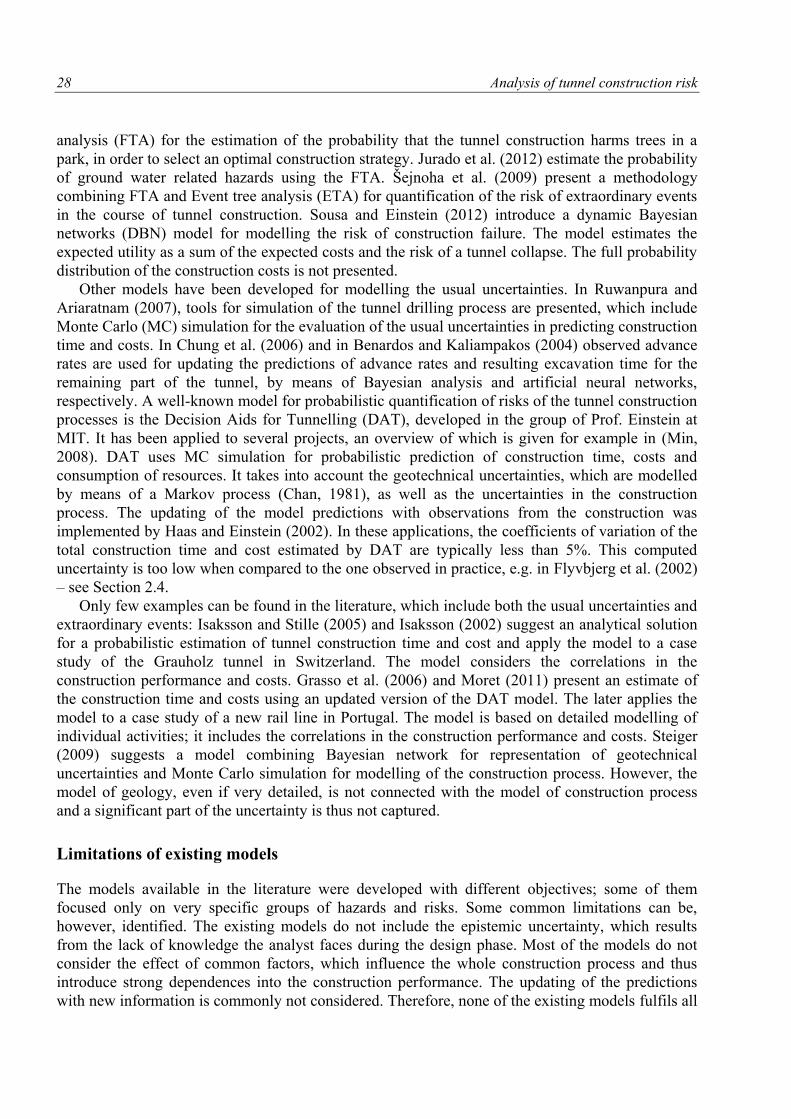
28 Analysis of tunnel construction risk
analysis (FTA) for the estimation of the probability that the tunnel construction harms trees in a
park, in order to select an optimal construction strategy. Jurado et al. (2012) estimate the probability
of ground water related hazards using the FTA. Šejnoha et al. (2009) present a methodology
combining FTA and Event tree analysis (ETA) for quantification of the risk of extraordinary events
in the course of tunnel construction. Sousa and Einstein (2012) introduce a dynamic Bayesian
networks (DBN) model for modelling the risk of construction failure. The model estimates the
expected utility as a sum of the expected costs and the risk of a tunnel collapse. The full probability
distribution of the construction costs is not presented.
Other models have been developed for modelling the usual uncertainties. In Ruwanpura and
Ariaratnam (2007), tools for simulation of the tunnel drilling process are presented, which include
Monte Carlo (MC) simulation for the evaluation of the usual uncertainties in predicting construction
time and costs. In Chung et al. (2006) and in Benardos and Kaliampakos (2004) observed advance
rates are used for updating the predictions of advance rates and resulting excavation time for the
remaining part of the tunnel, by means of Bayesian analysis and artificial neural networks,
respectively. A well-known model for probabilistic quantification of risks of the tunnel construction
processes is the Decision Aids for Tunnelling (DAT), developed in the group of Prof. Einstein at
MIT. It has been applied to several projects, an overview of which is given for example in (Min,
2008). DAT uses MC simulation for probabilistic prediction of construction time, costs and
consumption of resources. It takes into account the geotechnical uncertainties, which are modelled
by means of a Markov process (Chan, 1981), as well as the uncertainties in the construction
process. The updating of the model predictions with observations from the construction was
implemented by Haas and Einstein (2002). In these applications, the coefficients of variation of the
total construction time and cost estimated by DAT are typically less than 5%. This computed
uncertainty is too low when compared to the one observed in practice, e.g. in Flyvbjerg et al. (2002)
– see Section 2.4.
Only few examples can be found in the literature, which include both the usual uncertainties and
extraordinary events: Isaksson and Stille (2005) and Isaksson (2002) suggest an analytical solution
for a probabilistic estimation of tunnel construction time and cost and apply the model to a case
study of the Grauholz tunnel in Switzerland. The model considers the correlations in the
construction performance and costs. Grasso et al. (2006) and Moret (2011) present an estimate of
the construction time and costs using an updated version of the DAT model. The later applies the
model to a case study of a new rail line in Portugal. The model is based on detailed modelling of
individual activities; it includes the correlations in the construction performance and costs. Steiger
(2009) suggests a model combining Bayesian network for representation of geotechnical
uncertainties and Monte Carlo simulation for modelling of the construction process. However, the
model of geology, even if very detailed, is not connected with the model of construction process
and a significant part of the uncertainty is thus not captured.
Limitations of existing models
The models available in the literature were developed with different objectives; some of them
focused only on very specific groups of hazards and risks. Some common limitations can be,
however, identified. The existing models do not include the epistemic uncertainty, which results
from the lack of knowledge the analyst faces during the design phase. Most of the models do not
consider the effect of common factors, which influence the whole construction process and thus
introduce strong dependences into the construction performance. The updating of the predictions
with new information is commonly not considered. Therefore, none of the existing models fulfils all
29
requirements that are deemed important for a realistic estimation of construction time and costs;
these requirements are summarized later in Section 5. This shortages motivated the development of
Dynamic Bayesian Networks (DBN) model presented in this thesis.
Additionally, the existing models strongly rely on expert assessment of the input parameters.
These can be very unreliable, especially in assessing the variability and correlations of the
construction performance and in the prediction of rare events (Moret and Einstein, 2011a). No
systematic statistical analysis of the tunnel construction performance data, which might serve as a
basis for probabilistic modelling in the future tunnels, is available in the literature. Methodology for
such analysis is presented in Chapter 7.
3.3 Introduction to selected methods for uncertainty and risk
modelling
Principles of selected methods and models used for the quantitative analysis of the tunnel
construction risk are introduced in this section. The focus is on those, which are utilized later in this
thesis
The text assumes a basic knowledge of the probability theory, such as definition of random
events, random variables, probability distributions or random processes. A brief summary of
terminology, definitions and notation is given in Annex 1. For obtaining a complex theoretical
background, publications Benjamin and Cornell (1970), Melchers (1987) and Kottegoda and Rosso
(2008) are recommended.
3.3.1 Fault tree analysis (FTA)
FTA is a technique for analysis of the causes and estimation of the probability of an undesired event
(a top event in the FTA terminology). The top event corresponds to a particular failure mode of the
system (e.g. cave-in collapse). The fault tree (FT) itself is a graphical model displaying the
combinations of events (e.g. geotechnical faults or human error) that may result in the occurrence of
the top event. The method is in detailed described for example in Stewart and Melchers (1997) and
Stamatelatos and Vesely (2002).
FTA has an important disadvantage that is its limited ability to deal with dependent systems. In
classical FTs, the basic events are supposed to be statistically independent. The dependence
between particular events (random variables) can be included by repeating the branches of the tree
or by other advanced techniques. These methods, however, lead to exponential increase in the
complexity of the FT (Khakzad et al., 2011; Mahboob and Straub, 2011).
Because there are strong dependences between the events and phenomena leading to a tunnel
construction failure, the application of FTA for estimations of its probability is not very convenient.
For this reason, FTA is not discussed in this thesis. The technique is mentioned here, because it is
frequently used in the analysis of tunnel construction risks (see Section 3.2). The applications are
not likely to provide a reliable estimate of the probability of the failure. On the other hand,
application of FTA helps to understand and structuralize the problem and it can thus be beneficial
as a complementary method for the analysis of risks.
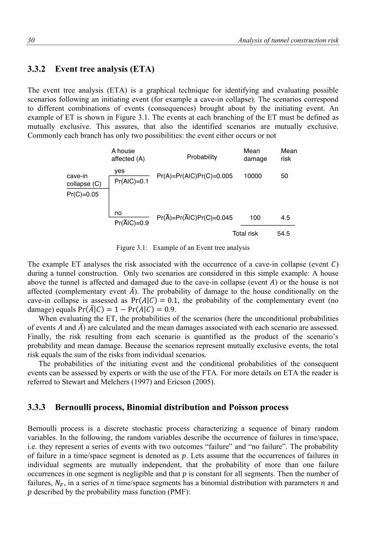
30 Analysis of tunnel construction risk
3.3.2 Event tree analysis (ETA)
The event tree analysis (ETA) is a graphical technique for identifying and evaluating possible
scenarios following an initiating event (for example a cave-in collapse). The scenarios correspond
to different combinations of events (consequences) brought about by the initiating event. An
example of ET is shown in Figure 3.1. The events at each branching of the ET must be defined as
mutually exclusive. This assures, that also the identified scenarios are mutually exclusive.
Commonly each branch has only two possibilities: the event either occurs or not
Figure 3.1: Example of an Event tree analysis
The example ET analyses the risk associated with the occurrence of a cave-in collapse (event )
during a tunnel construction. Only two scenarios are considered in this simple example: A house
above the tunnel is affected and damaged due to the cave-in collapse (event ) or the house is not
affected (complementary event ). The probability of damage to the house conditionally on the
cave-in collapse is assessed as | , the probability of the complementary event (no
damage) equals | | .
When evaluating the ET, the probabilities of the scenarios (here the unconditional probabilities
of events and ) are calculated and the mean damages associated with each scenario are assessed.
Finally, the risk resulting from each scenario is quantified as the product of the scenario’s
probability and mean damage. Because the scenarios represent mutually exclusive events, the total
risk equals the sum of the risks from individual scenarios.
The probabilities of the initiating event and the conditional probabilities of the consequent
events can be assessed by experts or with the use of the FTA. For more details on ETA the reader is
referred to Stewart and Melchers (1997) and Ericson (2005).
3.3.3 Bernoulli process, Binomial distribution and Poisson process
Bernoulli process is a discrete stochastic process characterizing a sequence of binary random
variables. In the following, the random variables describe the occurrence of failures in time/space,
i.e. they represent a series of events with two outcomes “failure” and “no failure”. The probability
of failure in a time/space segment is denoted as . Lets assume that the occurrences of failures in
individual segments are mutually independent, that the probability of more than one failure
occurrences in one segment is negligible and that is constant for all segments. Then the number of
failures, , in a series of time/space segments has a binomial distribution with parameters and
described by the probability mass function (PMF):
31
[ | ] (
) (3.1)
The expected number of failures, denoted as equals .
If the number of segments is large and the probability of failure in one segment is small, the
PMF of Eq. (3.1) can be approximated as follows
[ | ]
(3.2)
The expression in Eq. (3.2) is the PMF of the Poisson distribution with parameter . Both the
mean and variance of this distribution are equal to .
The Poisson process is a random process , whose value at time/in position is the
(random) number of failures, which occur in the interval ⟨ ⟩. The Poisson process is thus counting
the number of failures over time/space. The number of failures at time has the Poisson
distribution. To include the variable , it is convenient to write the PMF of Eq. (3.2) as
[ | ]
(3.3)
where is the parameter of the Poisson process. is commonly referred to as the average rate of
arrival, in case of failure modelling it is more specifically denoted as failure rate. It holds , where is the expected number of failures at time (position) .
The occurrence of failures must satisfy following assumptions to be representable by the
Poisson process (compare to the assumptions for the Bernoulli process stated above):
The failure rate does not change in time/space. A Poisson process fulfilling this assumption is called homogeneous.
The probability of two or more failures in a short segment of time/space is negligible. This assumption is easily fulfilled when rare events are modelled.
The number of failures in any interval of time is independent of the number of failures in any other nonoverlapping interval of time. Because of this property, the Poisson process is called memoryless; i.e. past observations do not influence the probability of future events.
In some cases the first assumption is not fulfilled and the parameter of the Poisson process, , changes in time/space. Then we speak about a nonhomogeneous Poisson process and the PMF of
number of failures at time equals
( ) (3.4)
where ∫
is the mean of the Poisson distribution.
If the occurrence of failures follows a homogeneous Poisson process, the time/space interval, ,
between two occurrences has an exponential distribution with parameter and probability density
function (PDF):
(3.5)
The Poisson process is used in many engineering applications (Cornell, 1968; Cooke and Jager,
1998; Ditlevsen, 2006; Yeo and Cornell, 2009). In Chapter 4 of this thesis it is applied for
32 Analysis of tunnel construction risk
modelling of failures emerging in the course of the tunnel construction. For more details about the
stochastic process and probabilistic models the reader is referred to Benjamin and Cornell (1970)
and Kottegoda and Rosso (2008).
3.3.4 Markov process
Markov process is a stochastic process having the Markov property. A stochastic process has a
Markov property, if at any point of the process the future behaviour of the system depends only on
the present state and not on the past states. This property is also called memorylessness.
A Markov process with discrete variables is called a Markov chain. The Markov chain is
commonly defined for discrete steps of time or space, i.e. the variables are changing from one step
to the other. Note that the Poisson process (Section 3.3.3) is a special case of the Markov chain.
A homogeneous Markov chain containing a sequence of discrete random variables
with states is defined by
The probability distribution of the initial state (
) [ ] .
The transition probabilities [ | ] , representing the probability that the variable is in the th state given that the variable at the previous step, , is in the th state.
In case of a non-homogeneous Markov chain, the transition probabilities change in time/space. In
the following, only the homogeneous Markov chain is considered.
The transition probabilities can be conveniently organized in a transition probability matrix
[
] (3.6)
and the marginal probability distribution of the variable can be organized in a state probability
row vector
[ (
) (
) (
)]. (3.7)
The probability distribution of in the th step of the Markov chain can be thus calculated as
(3.8)
The Markov processes are used in many engineering applications such as in deterioration modelling
and maintenance planning (Kobayashi et al., 2012) or fault detection and prognosis (Ge et al.,
2004). (Chan, 1981) suggests utilization of Markov process for modelling the geotechnical
conditions along the tunnel axis. This approach is applied to the DBN model presented in Chapter
5. For more details on the Markov processes and Markov’s chains the reader is referred to Parzen
(1962) or Benjamin and Cornell (1970).
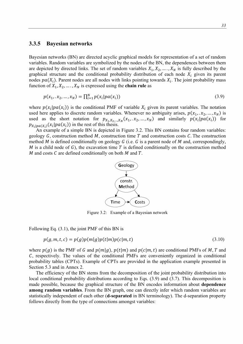
33
3.3.5 Bayesian networks
Bayesian networks (BN) are directed acyclic graphical models for representation of a set of random
variables. Random variables are symbolized by the nodes of the BN, the dependences between them
are depicted by directed links. The set of random variables is fully described by the
graphical structure and the conditional probability distribution of each node given its parent
nodes . Parent nodes are all nodes with links pointing towards . The joint probability mass
function of is expressed using the chain rule as
∏ | (3.9)
where | is the conditional PMF of variable given its parent variables. The notation
used here applies to discrete random variables. Whenever no ambiguity arises, is
used as the short notation for and similarly | for
| | in the rest of this thesis.
An example of a simple BN is depicted in Figure 3.2. This BN contains four random variables:
geology , construction method , construction time and construction costs The construction
method is defined conditionally on geology (i.e. is a parent node of and, correspondingly,
is a child node of ), the excavation time is defined conditionally on the construction method
and costs are defined conditionally on both and .
Figure 3.2: Example of a Bayesian network
Following Eq. (3.1), the joint PMF of this BN is
| | | (3.10)
where is the PMF of and | , | and | are conditional PMFs of , and
, respectively. The values of the conditional PMFs are conveniently organized in conditional
probability tables (CPTs). Example of CPTs are provided in the application example presented in
Section 5.3 and in Annex 2.
The efficiency of the BN stems from the decomposition of the joint probability distribution into
local conditional probability distributions according to Eqs. (3.9) and (3.7). This decomposition is
made possible, because the graphical structure of the BN encodes information about dependence
among random variables. From the BN graph, one can directly infer which random variables are
statistically independent of each other (d-separated in BN terminology). The d-separation property
follows directly from the type of connections amongst variables:
Time Costs
constr.Method
Geology
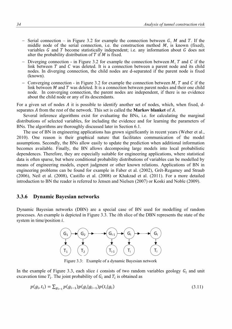
34 Analysis of tunnel construction risk
Serial connection – in Figure 3.2 for example the connection between , and . If the middle node of the serial connection, i.e. the construction method , is known (fixed), variables and become statistically independent; i.e. any information about does not alter the probability distribution of if is fixed.
Diverging connection - in Figure 3.2 for example the connection between , and if the link between and was deleted. It is a connection between a parent node and its child nodes. In diverging connection, the child nodes are d-separated if the parent node is fixed (known).
Converging connection - in Figure 3.2 for example the connection between , and if the link between and was deleted. It is a connection between parent nodes and their one child node. In converging connection, the parent nodes are independent, if there is no evidence about the child node or any of its descendants.
For a given set of nodes it is possible to identify another set of nodes, which, when fixed, d-
separates from the rest of the network. This set is called the Markov blanket of .
Several inference algorithms exist for evaluating the BNs, i.e. for calculating the marginal
distributions of selected variables, for including the evidence and for learning the parameters of
BNs. The algorithms are thoroughly discussed later in Section 6.1.
The use of BN in engineering applications has grown significantly in recent years (Weber et al.,
2010). One reason is their graphical nature that facilitates communication of the model
assumptions. Secondly, the BNs allow easily to update the prediction when additional information
becomes available. Finally, the BN allows decomposing large models into local probabilistic
dependences. Therefore, they are especially suitable for engineering applications, where statistical
data is often sparse, but where conditional probability distributions of variables can be modelled by
means of engineering models, expert judgment or other known relations. Applications of BN in
engineering problems can be found for example in Faber et al. (2002), Grêt-Regamey and Straub
(2006), Neil et al. (2008), Castillo et al. (2008) or Khakzad et al. (2011). For a more detailed
introduction to BN the reader is referred to Jensen and Nielsen (2007) or Koski and Noble (2009).
3.3.6 Dynamic Bayesian networks
Dynamic Bayesian networks (DBN) are a special case of BN used for modelling of random
processes. An example is depicted in Figure 3.3. The th slice of the DBN represents the state of the
system in time/position .
Figure 3.3: Example of a dynamic Bayesian network
In the example of Figure 3.3, each slice consists of two random variables geology and unit
excavation time . The joint probability of and is obtained as
∑ | | (3.11)
GI
TI
Gi-1
Ti-1
Gi
Ti
G2
T2
G1
T1
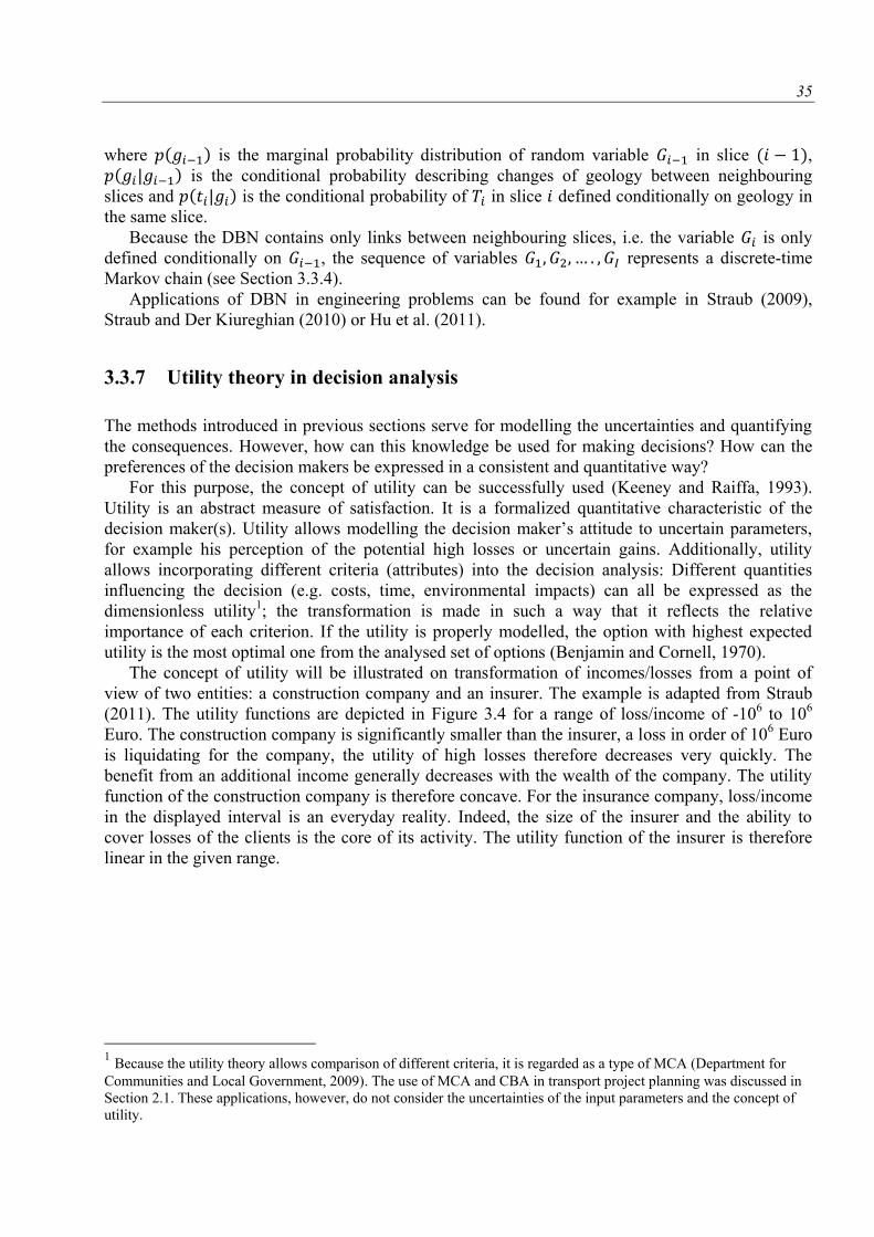
35
where is the marginal probability distribution of random variable in slice , | is the conditional probability describing changes of geology between neighbouring
slices and | is the conditional probability of in slice defined conditionally on geology in
the same slice.
Because the DBN contains only links between neighbouring slices, i.e. the variable is only
defined conditionally on , the sequence of variables represents a discrete-time
Markov chain (see Section 3.3.4).
Applications of DBN in engineering problems can be found for example in Straub (2009),
Straub and Der Kiureghian (2010) or Hu et al. (2011).
3.3.7 Utility theory in decision analysis
The methods introduced in previous sections serve for modelling the uncertainties and quantifying
the consequences. However, how can this knowledge be used for making decisions? How can the
preferences of the decision makers be expressed in a consistent and quantitative way?
For this purpose, the concept of utility can be successfully used (Keeney and Raiffa, 1993).
Utility is an abstract measure of satisfaction. It is a formalized quantitative characteristic of the
decision maker(s). Utility allows modelling the decision maker’s attitude to uncertain parameters,
for example his perception of the potential high losses or uncertain gains. Additionally, utility
allows incorporating different criteria (attributes) into the decision analysis: Different quantities
influencing the decision (e.g. costs, time, environmental impacts) can all be expressed as the
dimensionless utility1; the transformation is made in such a way that it reflects the relative
importance of each criterion. If the utility is properly modelled, the option with highest expected
utility is the most optimal one from the analysed set of options (Benjamin and Cornell, 1970).
The concept of utility will be illustrated on transformation of incomes/losses from a point of
view of two entities: a construction company and an insurer. The example is adapted from Straub
(2011). The utility functions are depicted in Figure 3.4 for a range of loss/income of -106 to 10
6
Euro. The construction company is significantly smaller than the insurer, a loss in order of 106 Euro
is liquidating for the company, the utility of high losses therefore decreases very quickly. The
benefit from an additional income generally decreases with the wealth of the company. The utility
function of the construction company is therefore concave. For the insurance company, loss/income
in the displayed interval is an everyday reality. Indeed, the size of the insurer and the ability to
cover losses of the clients is the core of its activity. The utility function of the insurer is therefore
linear in the given range.
1 Because the utility theory allows comparison of different criteria, it is regarded as a type of MCA (Department for
Communities and Local Government, 2009). The use of MCA and CBA in transport project planning was discussed in
Section 2.1. These applications, however, do not consider the uncertainties of the input parameters and the concept of
utility.
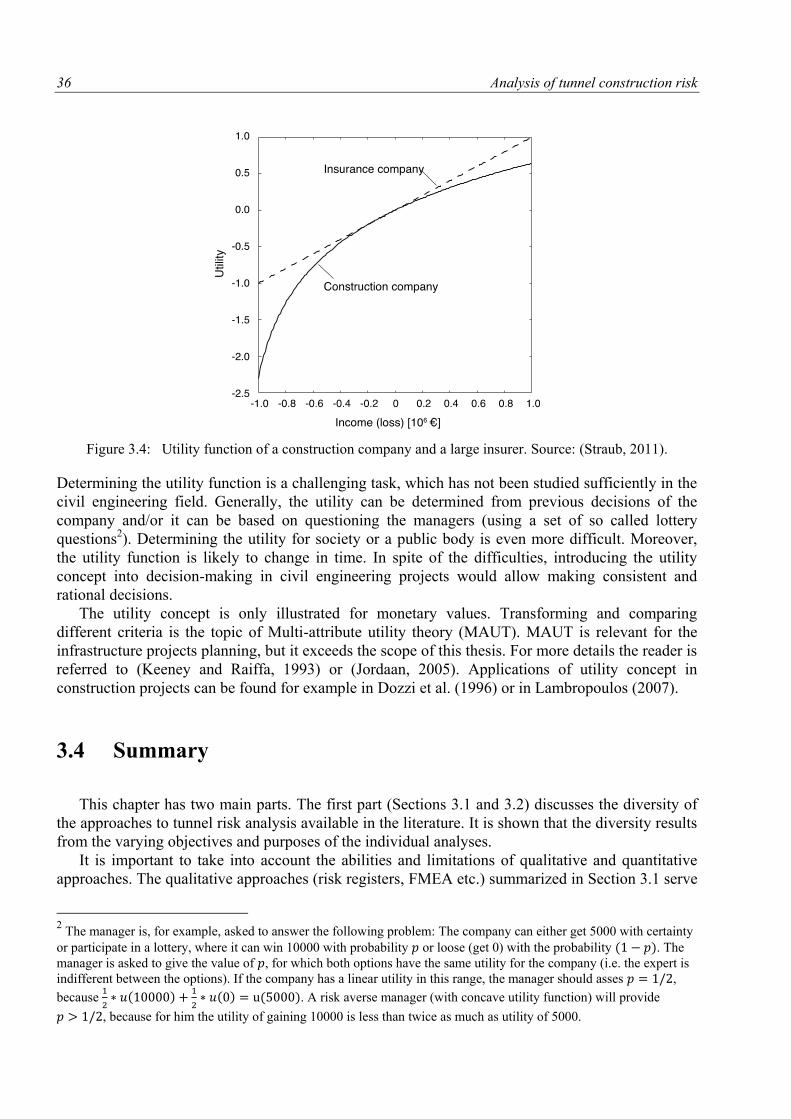
36 Analysis of tunnel construction risk
Figure 3.4: Utility function of a construction company and a large insurer. Source: (Straub, 2011).
Determining the utility function is a challenging task, which has not been studied sufficiently in the
civil engineering field. Generally, the utility can be determined from previous decisions of the
company and/or it can be based on questioning the managers (using a set of so called lottery
questions2). Determining the utility for society or a public body is even more difficult. Moreover,
the utility function is likely to change in time. In spite of the difficulties, introducing the utility
concept into decision-making in civil engineering projects would allow making consistent and
rational decisions.
The utility concept is only illustrated for monetary values. Transforming and comparing
different criteria is the topic of Multi-attribute utility theory (MAUT). MAUT is relevant for the
infrastructure projects planning, but it exceeds the scope of this thesis. For more details the reader is
referred to (Keeney and Raiffa, 1993) or (Jordaan, 2005). Applications of utility concept in
construction projects can be found for example in Dozzi et al. (1996) or in Lambropoulos (2007).
3.4 Summary
This chapter has two main parts. The first part (Sections 3.1 and 3.2) discusses the diversity of
the approaches to tunnel risk analysis available in the literature. It is shown that the diversity results
from the varying objectives and purposes of the individual analyses.
It is important to take into account the abilities and limitations of qualitative and quantitative
approaches. The qualitative approaches (risk registers, FMEA etc.) summarized in Section 3.1 serve
2 The manager is, for example, asked to answer the following problem: The company can either get 5000 with certainty
or participate in a lottery, where it can win 10000 with probability or loose (get 0) with the probability . The
manager is asked to give the value of , for which both options have the same utility for the company (i.e. the expert is
indifferent between the options). If the company has a linear utility in this range, the manager should asses ,
because
. A risk averse manager (with concave utility function) will provide
, because for him the utility of gaining 10000 is less than twice as much as utility of 5000.
37
as a basis for project risk management, for prioritizing the hazards and risks, for developing risk
treatment strategies and for allocating the responsibilities. The identification of hazards carried out
within a qualitative analysis is a basis for risk quantification. However, because the qualitative
approaches do not take into consideration the interconnectivity and dependences amongst different
hazards, they cannot be used for quantitative estimate of the overall uncertainties and risks.
Consequently, for making an objective decision, quantitative approaches should always be used,
which model the complexity of the system. The quantitative estimates should also be presented to
public and stakeholders. The existing quantitative models are presented in Section 3.2 and their
limitations are discussed, which motivate the development of models presented in this thesis.
Second part of the chapter (Section 3.3) introduces the tools and methods, which are used in the
quantitative models presented later in the thesis. The principles of the methods are illustrated on
simple examples related to the tunnel construction. Notation used throughout the thesis is
introduced here and in Annex 1.

39
In this chapter, a simple model for probabilistic modelling of delay caused by tunnel construction
failures is introduced. This model can be used as a complement to a deterministic estimate of
construction time and cost. The failure occurrence is modelled as inhomogeneous Poisson process
following the procedure described in Section 4.1.1. Consequences of the failures are assessed using
the Event Tree Analysis (ETA) as shown in Section 4.1.2.
The approach is applied to an application example in Section 4.2. The delay due to failures is
assessed for a secondary tunnel constructed as a part of underground system extension by a
conventional tunnelling method. The application example further illustrates the use of the
probabilistic estimate of delay for quantification of risk (Section 4.2.3) and for making decisions
(Section 4.2.4).
The proposed model was previously published in Špačková et al. (2010), where the utilization of
expert estimates of parameters of the Poisson model was discussed. The application example shown
in Section 4.2 was not previously presented.
4.1 Modelling delay due to failures - methodology
4.1.1 Number of failures
Following Eq. (3.3), the number of failures , which occur during the excavation of a tunnel
section with length , has Poisson distribution. The probability of occurrence of failures is
calculated as:
[ | ]
(4.1)
where is the failure rate, i.e. the number of failures per unit length.
4 Model of delay due to tunnel
construction failures and estimate of
associated risk
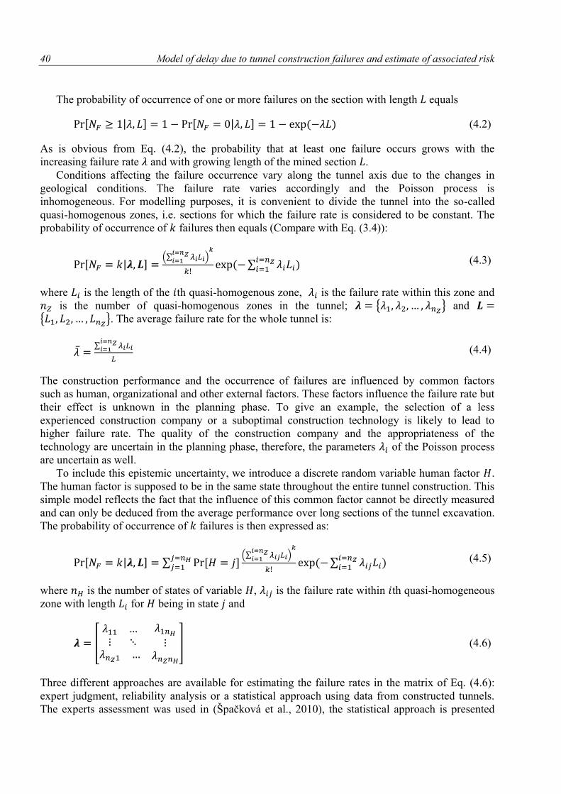
Model of delay due to tunnel construction failures and estimate of associated risk
40
The probability of occurrence of one or more failures on the section with length equals
[ | ] [ | ] (4.2)
As is obvious from Eq. (4.2), the probability that at least one failure occurs grows with the
increasing failure rate and with growing length of the mined section .
Conditions affecting the failure occurrence vary along the tunnel axis due to the changes in
geological conditions. The failure rate varies accordingly and the Poisson process is
inhomogeneous. For modelling purposes, it is convenient to divide the tunnel into the so-called
quasi-homogenous zones, i.e. sections for which the failure rate is considered to be constant. The
probability of occurrence of failures then equals (Compare with Eq. (3.4)):
[ | ] (∑
)
∑
(4.3)
where is the length of the th quasi-homogenous zone, is the failure rate within this zone and
is the number of quasi-homogenous zones in the tunnel; { } and
{ }. The average failure rate for the whole tunnel is:
∑
(4.4)
The construction performance and the occurrence of failures are influenced by common factors
such as human, organizational and other external factors. These factors influence the failure rate but
their effect is unknown in the planning phase. To give an example, the selection of a less
experienced construction company or a suboptimal construction technology is likely to lead to
higher failure rate. The quality of the construction company and the appropriateness of the
technology are uncertain in the planning phase, therefore, the parameters of the Poisson process
are uncertain as well.
To include this epistemic uncertainty, we introduce a discrete random variable human factor .
The human factor is supposed to be in the same state throughout the entire tunnel construction. This
simple model reflects the fact that the influence of this common factor cannot be directly measured
and can only be deduced from the average performance over long sections of the tunnel excavation.
The probability of occurrence of failures is then expressed as:
[ | ] ∑ [ ](∑
)
∑
(4.5)
where is the number of states of variable , is the failure rate within th quasi-homogeneous
zone with length for being in state and
[
] (4.6)
Three different approaches are available for estimating the failure rates in the matrix of Eq. (4.6):
expert judgment, reliability analysis or a statistical approach using data from constructed tunnels.
The experts assessment was used in (Špačková et al., 2010), the statistical approach is presented
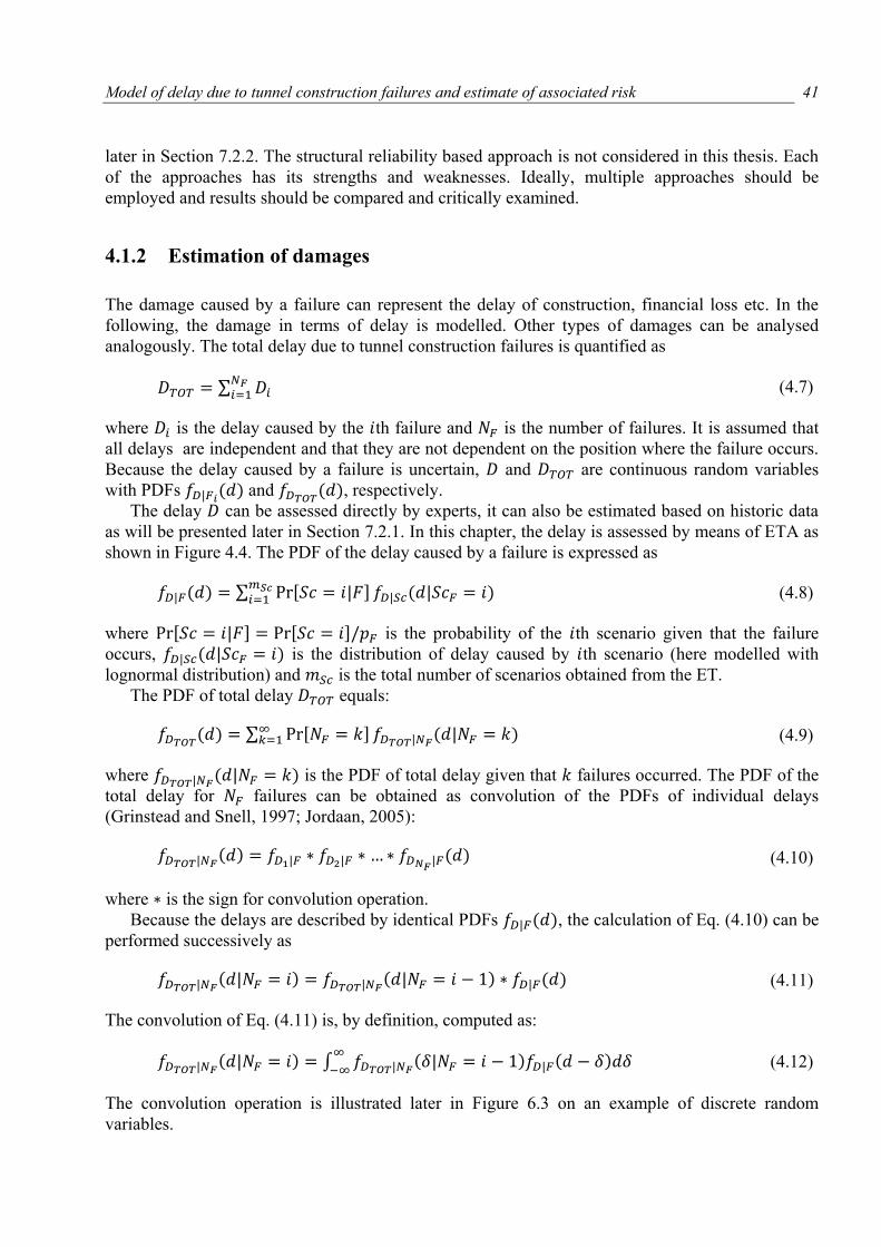
Model of delay due to tunnel construction failures and estimate of associated risk
41
later in Section 7.2.2. The structural reliability based approach is not considered in this thesis. Each
of the approaches has its strengths and weaknesses. Ideally, multiple approaches should be
employed and results should be compared and critically examined.
4.1.2 Estimation of damages
The damage caused by a failure can represent the delay of construction, financial loss etc. In the
following, the damage in terms of delay is modelled. Other types of damages can be analysed
analogously. The total delay due to tunnel construction failures is quantified as
∑ (4.7)
where is the delay caused by the th failure and is the number of failures. It is assumed that
all delays are independent and that they are not dependent on the position where the failure occurs.
Because the delay caused by a failure is uncertain, and are continuous random variables
with PDFs | and
, respectively.
The delay can be assessed directly by experts, it can also be estimated based on historic data
as will be presented later in Section 7.2.1. In this chapter, the delay is assessed by means of ETA as
shown in Figure 4.4. The PDF of the delay caused by a failure is expressed as
| ∑ [ | ] | | (4.8)
where [ | ] [ ] is the probability of the th scenario given that the failure
occurs, | | is the distribution of delay caused by th scenario (here modelled with
lognormal distribution) and is the total number of scenarios obtained from the ET.
The PDF of total delay equals:
∑ [ ]
| | (4.9)
where | | is the PDF of total delay given that failures occurred. The PDF of the
total delay for failures can be obtained as convolution of the PDFs of individual delays
(Grinstead and Snell, 1997; Jordaan, 2005):
| | |
| (4.10)
where is the sign for convolution operation.
Because the delays are described by identical PDFs | , the calculation of Eq. (4.10) can be
performed successively as
| | |
| | (4.11)
The convolution of Eq. (4.11) is, by definition, computed as:
| | ∫ |
| |
(4.12)
The convolution operation is illustrated later in Figure 6.3 on an example of discrete random
variables.
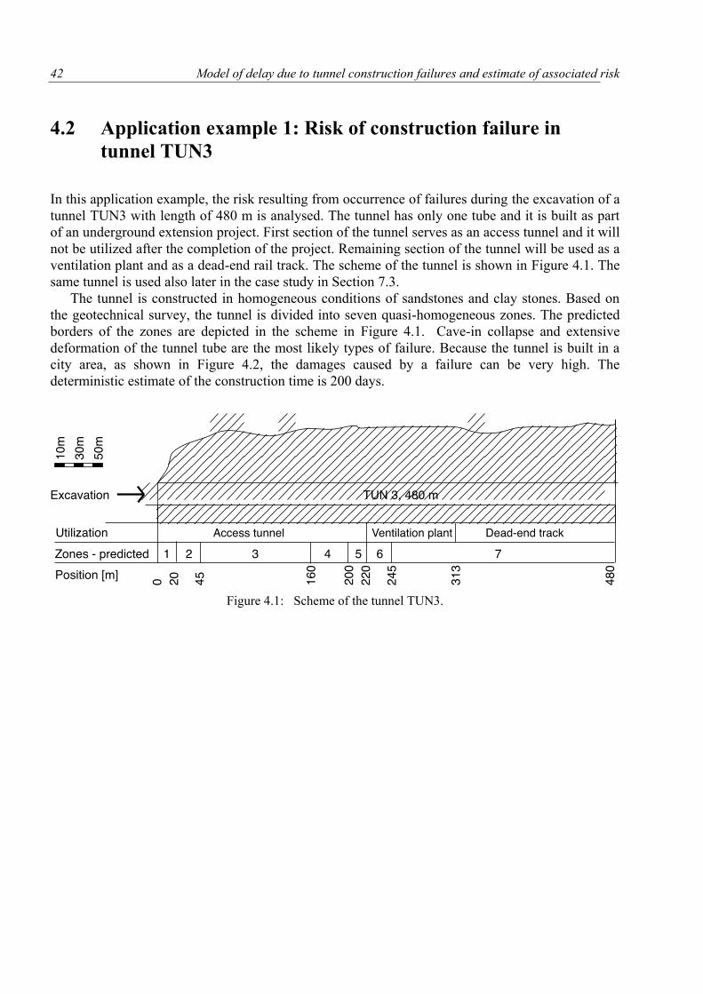
Model of delay due to tunnel construction failures and estimate of associated risk
42
4.2 Application example 1: Risk of construction failure in
tunnel TUN3
In this application example, the risk resulting from occurrence of failures during the excavation of a
tunnel TUN3 with length of 480 m is analysed. The tunnel has only one tube and it is built as part
of an underground extension project. First section of the tunnel serves as an access tunnel and it will
not be utilized after the completion of the project. Remaining section of the tunnel will be used as a
ventilation plant and as a dead-end rail track. The scheme of the tunnel is shown in Figure 4.1. The
same tunnel is used also later in the case study in Section 7.3.
The tunnel is constructed in homogeneous conditions of sandstones and clay stones. Based on
the geotechnical survey, the tunnel is divided into seven quasi-homogeneous zones. The predicted
borders of the zones are depicted in the scheme in Figure 4.1. Cave-in collapse and extensive
deformation of the tunnel tube are the most likely types of failure. Because the tunnel is built in a
city area, as shown in Figure 4.2, the damages caused by a failure can be very high. The
deterministic estimate of the construction time is 200 days.
Figure 4.1: Scheme of the tunnel TUN3.
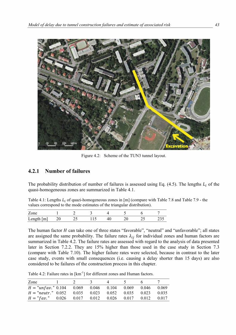
Model of delay due to tunnel construction failures and estimate of associated risk
43
Figure 4.2: Scheme of the TUN3 tunnel layout.
4.2.1 Number of failures
The probability distribution of number of failures is assessed using Eq. (4.5). The lengths of the
quasi-homogeneous zones are summarized in Table 4.1.
Table 4.1: Lengths of quazi-homogeneous zones in [m] (compare with Table 7.8 and Table 7.9 - the
values correspond to the mode estimates of the triangular distribution).
Zone 1 2 3 4 5 6 7
Length [m] 20 25 115 40 20 25 235
The human factor can take one of three states “favorable”, “neutral” and “unfavorable”; all states
are assigned the same probability. The failure rates for individual zones and human factors are
summarized in Table 4.2. The failure rates are assessed with regard to the analysis of data presented
later in Section 7.2.2. They are 15% higher than those used in the case study in Section 7.3
(compare with Table 7.10). The higher failure rates were selected, because in contrast to the later
case study, events with small consequences (i.e. causing a delay shorter than 15 days) are also
considered to be failures of the construction process in this chapter.
Table 4.2: Failure rates in [km-1
] for different zones and Human factors.
Zone 1 2 3 4 5 6 7
0.104 0.069 0.046 0.104 0.069 0.046 0.069
0.052 0.035 0.023 0.052 0.035 0.023 0.035
0.026 0.017 0.012 0.026 0.017 0.012 0.017
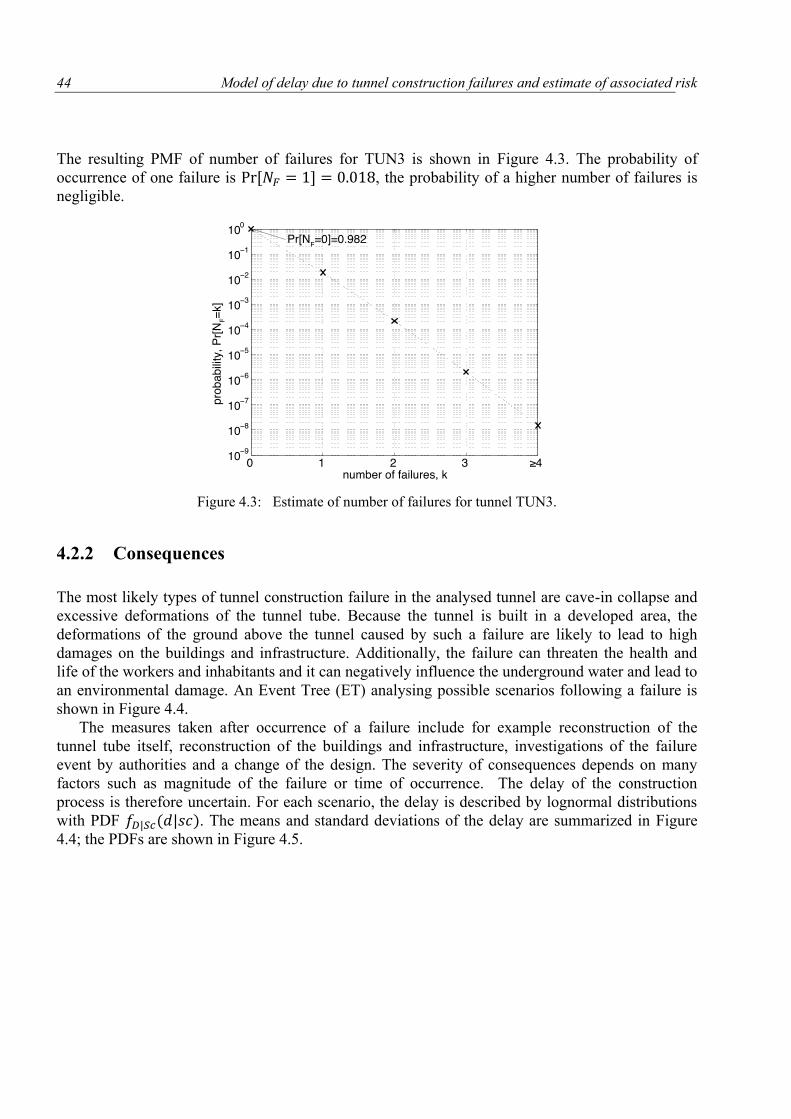
Model of delay due to tunnel construction failures and estimate of associated risk
44
The resulting PMF of number of failures for TUN3 is shown in Figure 4.3. The probability of
occurrence of one failure is [ ] , the probability of a higher number of failures is
negligible.
Figure 4.3: Estimate of number of failures for tunnel TUN3.
4.2.2 Consequences
The most likely types of tunnel construction failure in the analysed tunnel are cave-in collapse and
excessive deformations of the tunnel tube. Because the tunnel is built in a developed area, the
deformations of the ground above the tunnel caused by such a failure are likely to lead to high
damages on the buildings and infrastructure. Additionally, the failure can threaten the health and
life of the workers and inhabitants and it can negatively influence the underground water and lead to
an environmental damage. An Event Tree (ET) analysing possible scenarios following a failure is
shown in Figure 4.4.
The measures taken after occurrence of a failure include for example reconstruction of the
tunnel tube itself, reconstruction of the buildings and infrastructure, investigations of the failure
event by authorities and a change of the design. The severity of consequences depends on many
factors such as magnitude of the failure or time of occurrence. The delay of the construction
process is therefore uncertain. For each scenario, the delay is described by lognormal distributions
with PDF | | . The means and standard deviations of the delay are summarized in Figure
4.4; the PDFs are shown in Figure 4.5.
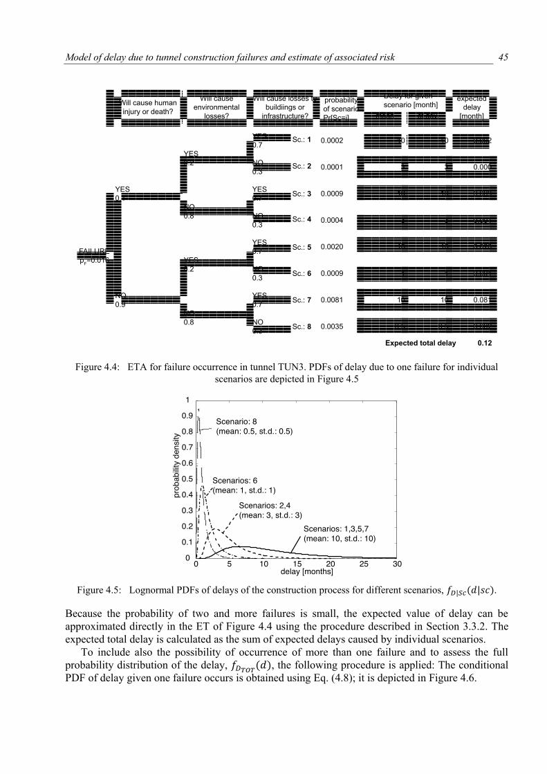
Model of delay due to tunnel construction failures and estimate of associated risk
45
Figure 4.4: ETA for failure occurrence in tunnel TUN3. PDFs of delay due to one failure for individual
scenarios are depicted in Figure 4.5
Figure 4.5: Lognormal PDFs of delays of the construction process for different scenarios, | | .
Because the probability of two and more failures is small, the expected value of delay can be
approximated directly in the ET of Figure 4.4 using the procedure described in Section 3.3.2. The
expected total delay is calculated as the sum of expected delays caused by individual scenarios.
To include also the possibility of occurrence of more than one failure and to assess the full
probability distribution of the delay, , the following procedure is applied: The conditional
PDF of delay given one failure occurs is obtained using Eq. (4.8); it is depicted in Figure 4.6.
mean st.dev.
YES
0.70.0002 10 10 0.002
YES
0.2 NO
0.30.0001 3 3 0.000
YES YES
0.1 0.70.0009 10 10 0.009
NO
0.8 NO
0.30.0004 3 3 0.001
YES
FAILURE 0.70.0020 10 10 0.020
pF=0.016 YES
0.2 NO
0.30.0009 1 1 0.001
NO YES
0.9 0.70.0081 10 10 0.081
NO
0.8 NO
0.30.0035 0.5 0.5 0.002
Expected total delay 0.12
Delay for given
scenario [month]Will cause human
injury or death?
Will cause
environmental
losses?
Will cause losses to
buildiings or
infrastructure?
probability
of scenario
Pr[Sc=i]
expected
delay
[month]
Sc.: 1
Sc.: 2
Sc.: 3
Sc.: 4
Sc.: 5
Sc.: 6
Sc.: 7
Sc.: 8
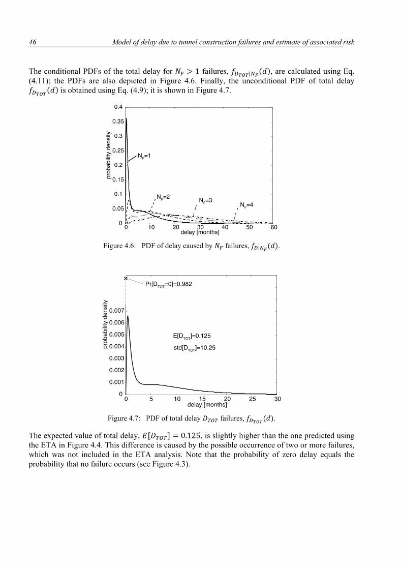
Model of delay due to tunnel construction failures and estimate of associated risk
46
The conditional PDFs of the total delay for failures, | , are calculated using Eq.
(4.11); the PDFs are also depicted in Figure 4.6. Finally, the unconditional PDF of total delay
is obtained using Eq. (4.9); it is shown in Figure 4.7.
Figure 4.6: PDF of delay caused by failures, | .
Figure 4.7: PDF of total delay failures, .
The expected value of total delay, [ ] , is slightly higher than the one predicted using
the ETA in Figure 4.4. This difference is caused by the possible occurrence of two or more failures,
which was not included in the ETA analysis. Note that the probability of zero delay equals the
probability that no failure occurs (see Figure 4.3).
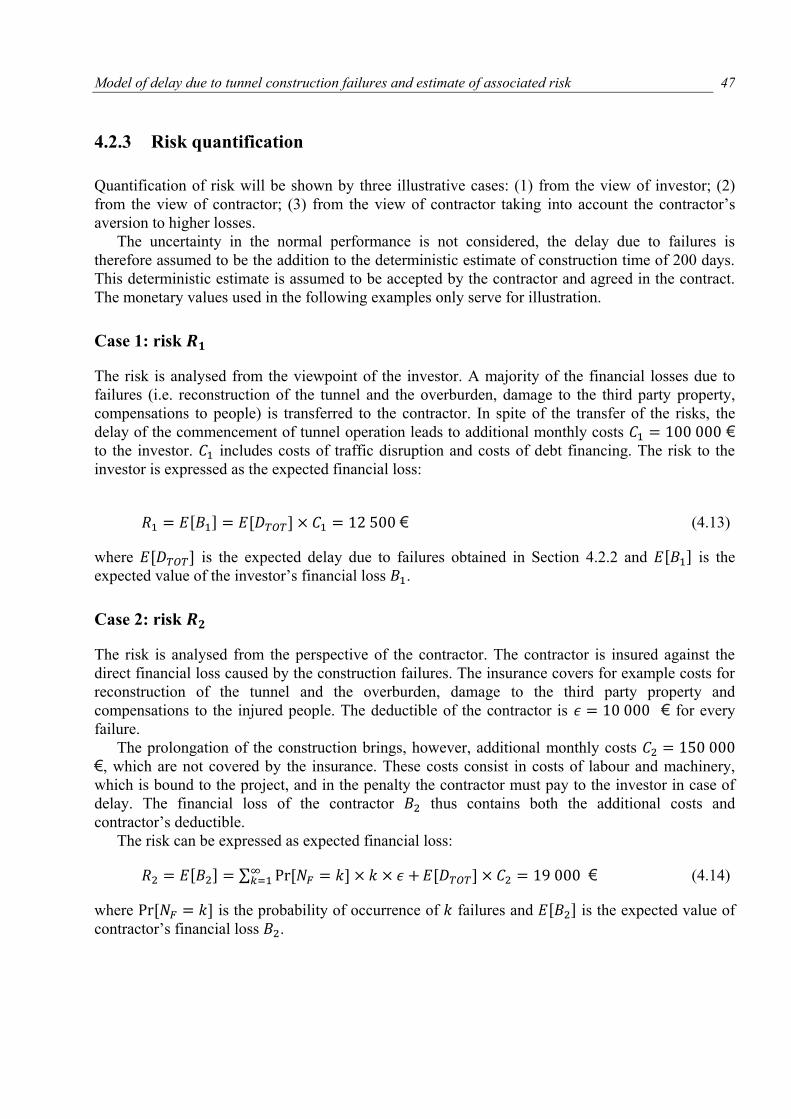
Model of delay due to tunnel construction failures and estimate of associated risk
47
4.2.3 Risk quantification
Quantification of risk will be shown by three illustrative cases: (1) from the view of investor; (2)
from the view of contractor; (3) from the view of contractor taking into account the contractor’s
aversion to higher losses.
The uncertainty in the normal performance is not considered, the delay due to failures is
therefore assumed to be the addition to the deterministic estimate of construction time of 200 days.
This deterministic estimate is assumed to be accepted by the contractor and agreed in the contract.
The monetary values used in the following examples only serve for illustration.
Case 1: risk
The risk is analysed from the viewpoint of the investor. A majority of the financial losses due to
failures (i.e. reconstruction of the tunnel and the overburden, damage to the third party property,
compensations to people) is transferred to the contractor. In spite of the transfer of the risks, the
delay of the commencement of tunnel operation leads to additional monthly costs €
to the investor. includes costs of traffic disruption and costs of debt financing. The risk to the
investor is expressed as the expected financial loss:
[ ] [ ] € (4.13)
where [ ] is the expected delay due to failures obtained in Section 4.2.2 and [ ] is the
expected value of the investor’s financial loss .
Case 2: risk
The risk is analysed from the perspective of the contractor. The contractor is insured against the
direct financial loss caused by the construction failures. The insurance covers for example costs for
reconstruction of the tunnel and the overburden, damage to the third party property and
compensations to the injured people. The deductible of the contractor is € for every
failure.
The prolongation of the construction brings, however, additional monthly costs
€, which are not covered by the insurance. These costs consist in costs of labour and machinery,
which is bound to the project, and in the penalty the contractor must pay to the investor in case of
delay. The financial loss of the contractor thus contains both the additional costs and
contractor’s deductible.
The risk can be expressed as expected financial loss:
[ ] ∑ [ ] [ ] € (4.14)
where [ ] is the probability of occurrence of failures and [ ] is the expected value of
contractor’s financial loss .
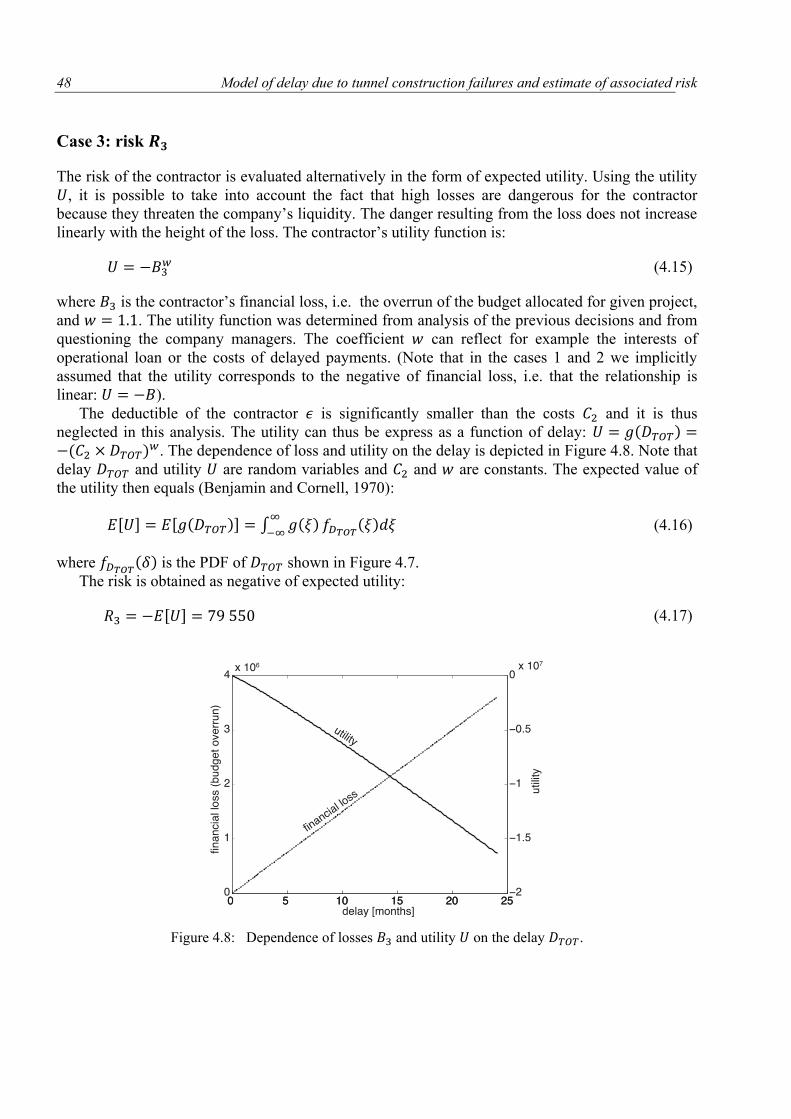
Model of delay due to tunnel construction failures and estimate of associated risk
48
Case 3: risk
The risk of the contractor is evaluated alternatively in the form of expected utility. Using the utility
, it is possible to take into account the fact that high losses are dangerous for the contractor
because they threaten the company’s liquidity. The danger resulting from the loss does not increase
linearly with the height of the loss. The contractor’s utility function is:
(4.15)
where is the contractor’s financial loss, i.e. the overrun of the budget allocated for given project,
and . The utility function was determined from analysis of the previous decisions and from
questioning the company managers. The coefficient can reflect for example the interests of
operational loan or the costs of delayed payments. (Note that in the cases 1 and 2 we implicitly
assumed that the utility corresponds to the negative of financial loss, i.e. that the relationship is
linear: ).
The deductible of the contractor is significantly smaller than the costs and it is thus
neglected in this analysis. The utility can thus be express as a function of delay:
. The dependence of loss and utility on the delay is depicted in Figure 4.8. Note that
delay and utility are random variables and and are constants. The expected value of
the utility then equals (Benjamin and Cornell, 1970):
[ ] [ ] ∫
(4.16)
where is the PDF of shown in Figure 4.7.
The risk is obtained as negative of expected utility:
[ ] (4.17)
Figure 4.8: Dependence of losses and utility on the delay .
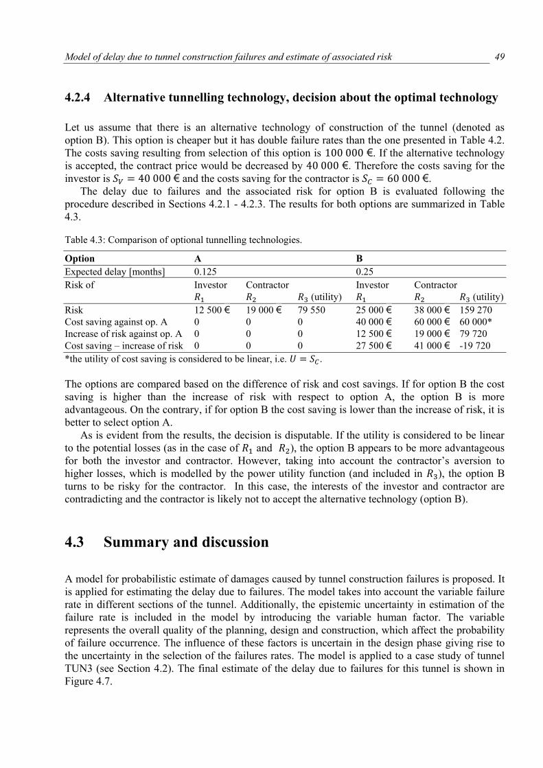
Model of delay due to tunnel construction failures and estimate of associated risk
49
4.2.4 Alternative tunnelling technology, decision about the optimal technology
Let us assume that there is an alternative technology of construction of the tunnel (denoted as
option B). This option is cheaper but it has double failure rates than the one presented in Table 4.2.
The costs saving resulting from selection of this option is €. If the alternative technology
is accepted, the contract price would be decreased by €. Therefore the costs saving for the
investor is € and the costs saving for the contractor is €.
The delay due to failures and the associated risk for option B is evaluated following the
procedure described in Sections 4.2.1 - 4.2.3. The results for both options are summarized in Table
4.3.
Table 4.3: Comparison of optional tunnelling technologies.
Option A B
Expected delay [months] 0.125 0.25
Risk of Investor Contractor Investor Contractor
(utility) (utility)
Risk 12 500 € 19 000 € 79 550 25 000 € 38 000 € 159 270
Cost saving against op. A 0 0 0 40 000 € 60 000 € 60 000*
Increase of risk against op. A 0 0 0 12 500 € 19 000 € 79 720
Cost saving – increase of risk 0 0 0 27 500 € 41 000 € -19 720
*the utility of cost saving is considered to be linear, i.e. .
The options are compared based on the difference of risk and cost savings. If for option B the cost
saving is higher than the increase of risk with respect to option A, the option B is more
advantageous. On the contrary, if for option B the cost saving is lower than the increase of risk, it is
better to select option A.
As is evident from the results, the decision is disputable. If the utility is considered to be linear
to the potential losses (as in the case of and ), the option B appears to be more advantageous
for both the investor and contractor. However, taking into account the contractor’s aversion to
higher losses, which is modelled by the power utility function (and included in ), the option B
turns to be risky for the contractor. In this case, the interests of the investor and contractor are
contradicting and the contractor is likely not to accept the alternative technology (option B).
4.3 Summary and discussion
A model for probabilistic estimate of damages caused by tunnel construction failures is proposed. It
is applied for estimating the delay due to failures. The model takes into account the variable failure
rate in different sections of the tunnel. Additionally, the epistemic uncertainty in estimation of the
failure rate is included in the model by introducing the variable human factor. The variable
represents the overall quality of the planning, design and construction, which affect the probability
of failure occurrence. The influence of these factors is uncertain in the design phase giving rise to
the uncertainty in the selection of the failures rates. The model is applied to a case study of tunnel
TUN3 (see Section 4.2). The final estimate of the delay due to failures for this tunnel is shown in
Figure 4.7.
Model of delay due to tunnel construction failures and estimate of associated risk
50
The estimated delay can be used for quantification of risk, as illustrated in Section 4.2.3. The
risk is quantified for three cases. In case 1 and 2, the risk is defined as the expected financial loss
(from the point of view of the investor and contractor, respectively). The loss is expressed as a
function of delay. For such analysis, only the estimate of expected value of the delay is needed. In
case 3, the risk is defined as negative expected utility. By introducing the utility the aversion of the
contractor to high financial losses can be taken into account. For modelling the utility, the full
probabilistic estimate of the delay is used.
Finally, an example decision-making process is presented in Section 4.2.4. Two alternative
tunnelling technologies are evaluated based on comparison of their risk and costs. It is shown that
the decision would differ for the two alternative definitions of risk (cases 2 and 3). For the case 3,
the risk aversion of the contractor outweighs the benefits from the cost savings.
The example of risk estimate and decision-making presented in this chapter aims at
demonstrating how the probabilistic estimates of construction time/cost should be utilized in the
tunnel project management. The results of the models presented later in this thesis might be utilized
in the same way. The selected monetary values as well as the utility function are purely illustrative.
In reality, other factors should be included in the decision making-process, the modelling of
construction costs should be improved and factors such as environmental or social impacts should
be included. A detailed investigation into the decision-making concepts is, however, beyond the
scope of this thesis.
51
A complex model for modelling of the tunnel construction time is presented in this section. The
main requirements on the model are the following: (1) It should consider both types of
uncertainties, i.e. the usual variability of the construction process and the extraordinary events – see
Section 2.7. (2) The model should consider the common factors that systematically influence the
construction process, such as human and organizational factors. These factors introduce stochastic
dependence into the performance at different phases of the construction. The significant influence
of such dependences on construction performance estimates is shown for example in van Dorp
(2005), Yang (2007) and Moret and Einstein (2011). (3) The model should allow for making full
use of data available from previous projects, such as advance rates and costs recorded during
excavation of tunnels under similar conditions. In this way, the know-how can be systematically
managed. (4) The methodology should facilitate the easy updating of predictions when new
information on the analysed project (e.g. geotechnical investigations, advance rates and costs
observed after commencement of excavation) is available. (5) The model assumptions and involved
simplifications must be properly understood and described. This is important in probabilistic
modelling where results are difficult to validate by experiments and must therefore be well
reasoned.
Many of the requirements could be satisfied by means of the commonly used MC simulation
based or analytical approaches. One can model the occurrence of both types of uncertainties
(requirement 1), it is also possible to include the dependences introduced by common factors
(requirement 2). The DAT model (Einstein, 1996) or the models by Isaksson and Stille, 2005) and
by Steiger (2009) can fulfil these requirements – see Section 3.2. Updating of the predictions
(requirement 4) based on observed performance during the tunnel construction has been also
presented in the literature, usually by means of Bayesian analysis (Chung et al., 2006).
5 Dynamic Bayesian network (DBN)
model of tunnel construction process
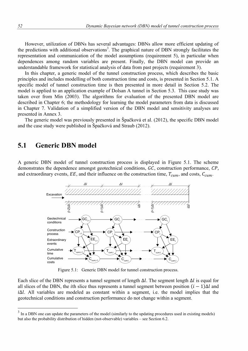
52 Dynamic Bayesian network (DBN) model of tunnel construction process
However, utilization of DBNs has several advantages: DBNs allow more efficient updating of
the predictions with additional observations3. The graphical nature of DBN strongly facilitates the
representation and communication of the model assumptions (requirement 5), in particular when
dependences among random variables are present. Finally, the DBN model can provide an
understandable framework for statistical analysis of data from past projects (requirement 3).
In this chapter, a generic model of the tunnel construction process, which describes the basic
principles and includes modelling of both construction time and costs, is presented in Section 5.1. A
specific model of tunnel construction time is then presented in more detail in Section 5.2. The
model is applied to an application example of Dolsan A tunnel in Section 5.3. This case study was
taken over from Min (2003). The algorithms for evaluation of the presented DBN model are
described in Chapter 6; the methodology for learning the model parameters from data is discussed
in Chapter 7. Validation of a simplified version of the DBN model and sensitivity analyses are
presented in Annex 3.
The generic model was previously presented in Špačková et al. (2012), the specific DBN model
and the case study were published in Špačková and Straub (2012).
5.1 Generic DBN model
A generic DBN model of tunnel construction process is displayed in Figure 5.1. The scheme
demonstrates the dependence amongst geotechnical conditions, , construction performance, and extraordinary events, , and their influence on the construction time, , and costs, .
Figure 5.1: Generic DBN model for tunnel construction process.
Each slice of the DBN represents a tunnel segment of length . The segment length is equal for
all slices of the DBN, the th slice thus represents a tunnel segment between position and
. All variables are modeled as constant within a segment, i.e. the model implies that the
geotechnical conditions and construction performance do not change within a segment.
3 In a DBN one can update the parameters of the model (similarly to the updating procedures used in existing models)
but also the probability distribution of hidden (not-observable) variables – see Section 6.2.
Dynamic Bayesian network (DBN) model of tunnel construction process 53
In a specific model, the geotechnical conditions, construction performance, as well as
extraordinary events are described in more detail by sets of random variables reflecting the tunnel
specifics. The selection of the appropriate set of variables depends on local geological conditions,
construction technology, routines and experiences of the owner, designer and constructor and on
information available in the time of the analysis. The levels of detailing in the modelling of
individual aspects should be balanced. For example, a detailed model of geotechnical conditions is
not beneficial for the time/cost prediction, if an accurate model of the associated construction
performance does not accompany it.
The modelling of different tunnels will mainly vary in the representation geotechnical
conditions. The general approach to their modelling is described in Sections 5.1.1 the specific
examples are shown in application examples in Sections 5.3 and 7.3. The modelling approaches for
construction performance and extraordinary events described in Section 5.1.2 and 5.1.3 are
generally applicable. The probabilistic definitions of the variables is shown in Section 5.2.
5.1.1 Geotechnical conditions
The area of the tunnel is first divided into zones, in which the ground has homogeneous
geotechnical properties. Within each zone, the properties are modelled as a homogeneous stochastic
process (as shown in the application example in Section 5.3) or as constant (as shown in application
example in Section 7.3). The location of the zone boundaries is uncertain, a random variable zone
introduces this uncertainty into the model.
The geotechnical properties can be modelled on different levels of detail: The selected variables
can either represent individual properties of the ground (e.g. lithology, discontinuities, water
content, presence of boulders) or they can correspond to a chosen geotechnical classification system
(RMR or Q class etc.).
Modelling of geotechnical properties by means of spatial Markov process is suggested in (Chan,
1981) and later utilized in other applications of the DAT model (see Section 3.2). Geotechnical
properties such as lithology, faulting or rock class are modelled as Markov process in the DAT
model (Einstein, 1996). The model assumes that the geotechnical parameters follow exponential
distribution, i.e. that the changes occur as a Poisson process. Statistical investigations into
geotechnical parameters available in the literature show that thickness of ground layers in sediments
follows an exponential, power law or lognormal distribution (Chakraborty et al., 2002; Longhitano
and Nemec, 2005; Felletti and Bersezio, 2010), distance of boulders follows exponential
distribution (Ditlevsen, 2006). For other geotechnical parameters, no statistical analysis is available
in the literature. The DBN model presented in this chapter takes over the modelling procedures of
DAT, the assumptions on the Poisson distribution of changes of the geological conditions should
be, however, proven in the future.
A summarizing variable, denoted as ground class, is defined conditionally on the other
variables used for representing geotechnical conditions. The ground class has direct correspondence
to the utilized technology of excavation and support pattern, i.e. it should reflect all the geotechnical
and hydrological conditions that influence the selection of construction method and thus the speed
and price of the construction as discussed in Section 2.4.
54 Dynamic Bayesian network (DBN) model of tunnel construction process
5.1.2 Construction performance
Construction performance is modelled by variables representing the tunnel geometry, construction
method, human factor and unit time4.
Geometry is a variable modelling the varying cross-section of the tunnel (e.g. typical cross-
section vs. extended cross-section for emergency parking places). The variable can also be used to
model inclination of the tunnel, special requirements on the excavation at the beginning and end of
the tunnel or in the position, where the tunnel passes other structures.
The variable construction method represents the applied excavation method, round length and
support pattern. The construction method is selected based on the ground class and tunnel
geometry.
In reality, the selection of the construction method also depends on the method utilized in the
previous segments, because the change of methods is commonly connected with additional costs
and time. In every cycle of the construction, a decision on optimal construction method must be
made with regard to actual construction method and to the actual and expected geotechnical
conditions. These decisions are made under high uncertainty. Techniques of modelling of such
decision problem exist, it is for example possible to combine DBNs with decision nodes. Such
model was presented for example in (Sousa, 2010), but with highly simplified assumptions.
Combination of the DBN suggested in this thesis with decision nodes would be computationally
very demanding and therefore not suitable for the real-time prediction and updating. The
applications presented in Section 5.3 and 7.3 are thus based on the assumption that the construction
methods can be changed any time and these changes are not associated with additional time.
The variable human factor reflects the influence of common factors, which systematically
influence the construction process and thus introduce strong stochastic dependences among the
performance in each segment of the tunnel. These can be the quality of design and planning,
organization of construction works or other external influences not included in other model
variables. The variable human factor can also be interpreted as the uncertainty in selection of the
appropriate probabilistic model (probability distribution) of unit time and failure rate, similar to the
approach described in Cheung and Beck (2010) and used in Section 4.1.1. To give an example, the
selection of a less experienced construction company or a suboptimal technology of the excavation
is likely to lead to a slower and more variable excavation process in many or all segments of the
tunnel. The quality of the construction company and the appropriateness of the technology are
uncertain in the planning phase. The uncertainty in these common factors and the resulting
uncertainty of the probability model of unit time increase the uncertainty in estimates of the total
construction time.
The human factor is supposed to be in the same state throughout the entire tunnel construction.
After the construction starts, human factor can be updated based on observed performance, i.e. the
probability of the most suitable probability distribution of unit time is increasing.
The unit time represents the time for excavation of a tunnel segment with length . It
corresponds to an inverse of the commonly used advance rate as will be discussed later in Section
7.1.1. The unit time is dependent on the construction method and on the human factor. The
probabilistic distribution of unit time can be assessed by experts but recommendably it should be
based on analysis of data from other excavated tunnels as discussed in Section 7.1.
4 The definition of variables described in this section applies to the conventional tunnelling method (see Section 2.2). In
case of mechanized tunnelling, definition of some variables might require adjustments.
Dynamic Bayesian network (DBN) model of tunnel construction process 55
The unit costs represent the costs for excavation of a tunnel segment with length . The costs
depend partly on the volume of works (material costs), and partly on the construction time (labour
costs, machinery costs). In the model, they are defined based on the construction method, human
factor and unit time. In the application examples in this thesis, the modelling of costs is not
discussed. Including the construction costs increases the complexity of the model and the
computational effort significantly. Additionally, no reliable data on construction costs are available
to the author.
5.1.3 Extraordinary events
For the modelling purposes, the extraordinary events are defined as events that cause a delay higher
than a threshold value (here selected equal to 15 days). The extraordinary events can represent for
example a cave-in collapse, tunnel flooding or severe legislative or public obstructions.
The occurrence of a failure is represented by a variable failure mode and it is defined
conditionally on the ground class and human factor. In the application examples in this thesis, the
different types of failure modes are not distinguished; the variable has only two states “failure” and
“no failure”. The probability of failure occurrence is calculated from the failure rates, i.e. the
number of failures per unit length of the tunnel. The assessment of the failure rate from data is
discussed in Section 7.2.2.
The variable number of failures represents the cumulative number of failures, which occurred
from the beginning of the tunnel excavation. It corresponds to the variable introduced in the
previous chapter (Section 4.1.1).
5.1.4 Length of segment represented by a slice of DBN
By choosing a slice length in the DBN model, implicit assumptions about dependences among the variables along the tunnel are made. In the model, changes of conditions can only occur between slices. Therefore, must be sufficiently small to capture the variability of geotechnical conditions along the tunnel axis (see Špačková and Straub, 2011). However, accurate modelling of geotechnical variability is not the only and main criterion.
Because the model assumes that the construction method in slice is determined purely based
on ground class and geometry, it implies full flexibility in changing construction methods between
slices. In reality, construction methods are only changed between excavation rounds (in case of
conventional tunnelling). Therefore, for the model to be realistic, the slice length should not be
shorter than the length of the round length.
5.2 Specific DBN model
A specific DBN model used for the tunnel construction process is depicted in Figure 5.2, an
overview of model variables is given in Table 5.1. The definition of the random variables is
discussed in the following.
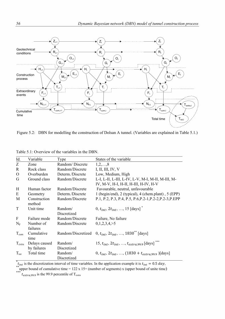
56 Dynamic Bayesian network (DBN) model of tunnel construction process
Figure 5.2: DBN for modelling the construction of Dolsan A tunnel. (Variables are explained in Table 5.1.)
Table 5.1: Overview of the variables in the DBN.
Id. Variable Type States of the variable
Z Zone Random/ Discrete 1,2,…,8
R Rock class Random/Discrete I, II, III, IV, V
O Overburden Determ./Discrete Low, Medium, High
G Ground class Random/Discrete L-I, L-II, L-III, L-IV, L-V, M-I, M-II, M-III, M-
IV, M-V, H-I, H-II, H-III, H-IV, H-V
H Human factor Random/Discrete Favourable, neutral, unfavourable
E Geometry Determ./Discrete 1 (begin/end), 2 (typical), 4 (chem.plant) , 5 (EPP)
M Construction
method
Random/Discrete P.1, P.2, P.3, P.4, P.5, P.6,P.2-1,P.2-2,P.2-3,P.EPP
T Unit time Random/
Discretized
0, , , …, 15 [days] *
F Failure mode Random/Discrete Failure, No failure
NF Number of
failures
Random/Discrete 0,1,2,3,4,>5
Tcum Cumulative
time
Random/Discretized 0, , , …, ** [days]
Textra Delays caused
by failures
Random/
Discretized
15, , , …, [days] ***
Ttot Total time Random/
Discretized
0, , , …, )[days]
* is the discretization interval of time variables. In the application example it is ,
**upper bound of cumulative time = 122 x 15= (number of segments) x (upper bound of unite time)
*** is the 99.9 percentile of Textra
Dynamic Bayesian network (DBN) model of tunnel construction process 57
5.2.1 Zone
The variable represents the position of a tunnel segment in quasi-homogenous geotechnical zones
along the tunnel axis. The uncertainty in the location of the boundary between zones and
is described by the CDF of the location of the boundary, . To establish the conditional PMF
of , let denote the probability that segment is part of zone j and the
probability that segment lies in zone j. Assuming that a segment can only be in either zone or zone , the probability of the th segment being in zone is calculated as
(
) (5.1)
where is the length of the segment represented by one slice of the DBN.
The conditional probabilities defining the variable (i.e. the values in the CPT) are:
|
(5.2)
| |
(5.3)
| (5.4)
If the segment can be in more than two different zones (e.g. in zone , and ), Eq. (5.1)-
(5.4) must be extended.
5.2.2 Rock class
The rock class describes the geotechnical conditions along the tunnel axis. In a zone it is
modeled as a Markov process. Parameters of the continuous Markov process are obtained from
experts in form of the average length
for which the rock class remains in state and transition
probabilities
, i.e. probability that, in case of a change, rock class is followed by rock class .
This definition follows the application of the DAT model in Chan (1981) resp. Min (2003)5.
In the DBN model, the Markov process is discretized into a Markov chain, i.e. it is transformed
to a discrete space represented by slices of the DBN corresponding to segments of length . Assuming that changes in rock class occur as a Poisson process, the conditional probabilities of
rock class in segment , , are derived from the parameters of the continuous Markov process as
follows:
5 Note, that the definition of transition probabilities
for continuous Markov process differs from the definition of
transition probabilities for discrete-time Markov chain, which is presented in Section 3.3.4 and used in the DBN model.
In the continuous Markov process, the transition probability is conditioned by the change of the state, i.e. the probability
of transition to the same state equals zero:
. This definition seems to be more intuitive and thus
more easily understandable for the experts.
58 Dynamic Bayesian network (DBN) model of tunnel construction process
| (
) (5.5)
|
⌈ (
)⌉ (5.6)
Note that due to the dependence introduced through the parent variables , the rock class is not a
Markov process. (It is a Markov process only conditional on zone .)
5.2.3 Overburden and Ground class
The variable representing the height of overburden can take three states: “low”, “medium” and
“high”. The variable is deterministic and it is defined as:
[ ] and [ ] if the mid-point of the th segment lies in the area with the low overburden,
[ ] and [ ] if the mid-point of the th segment lies in the area with the medium overburden,
[ ] and [ ] if the mid-point of the th segment lies in the area with the high overburden.
The ground class is defined deterministically for given and . As evident from Table 5.1,
each corresponds to a specific combination of and , e.g. ground class L-I stands for rock
class I with low overburden, H-II for rock class II with high overburden. Therefore:
[ | low and [ | low .
[ | high and [ | high .
Etc.
5.2.4 Variables describing construction performance
The variable Human factor , which represents the common factors influencing the construction
performance (see Section 5.1.2) is in one of the three states “unfavourable”, “neutral” or
“favourable” throughout the entire tunnel construction, i.e. the s are fully dependent from one
slice to the next and the conditional probability matrix | in each slice is the 3x3 identity
matrix.
The variable geometry is deterministic and it models different cross-sections along the tunnel
(a typical cross-section vs. extended cross-section for emergency parking places EPP), the special
conditions at the beginning and end of the tunnel and at the location where the tunnel passes an
existing chemical plant. The definition of the conditional probabilities of the variable is
analogous with that of the variable overburden.
The construction method describes the excavation type and the related support pattern
applied in the th segment and is determined conditional on the ground class and tunnel geometry
. The conditional probabilities of follow (Min, 2003) and they are summarized in Annex 2.
Dynamic Bayesian network (DBN) model of tunnel construction process 59
For every construction method and human factor , the unit time is defined by a
conditional CDF, | . To facilitate the application of the exact inference algorithm which
will be presented later in Section 6.2, the variable is discretized.
5.2.5 Failure mode
The variable failure mode represents the possible occurrence of an extraordinary event in
segment , it is defined conditionally on and . Assuming that failures occur as a Poisson
process for given and , in accordance with the Poisson model presented in Section 4.1.1, the
conditional probability of failure mode within a section of length can be approximated by:
| ( | ) (5.7)
| ( | ) (5.8)
where | is the conditional failure rate (corresponds to the failure rate in Section 4.1.1).
5.2.6 Number of failures
Number of failures represents the total number of failures from the beginning of the tunnel up
to the segment . With being the maximal number of failures to be considered (where state
represents or more failures), the conditional probabilities are:
( | ) , for { } , (5.9)
( | ) , for { } , (5.10)
( | ) . (5.11)
For all other conditional probabilities it holds
( | ) (5.12)
5.2.7 Construction time
The main output of the model is the total construction time, . In the DBN, it is computed as the
sum of construction time excluding extraordinary events, , and the time delay caused by
extraordinary events, .
The cumulative time is the time needed for the excavation of the tunnel up to the location
. It is defined as the sum of and the unit time in segment , : .
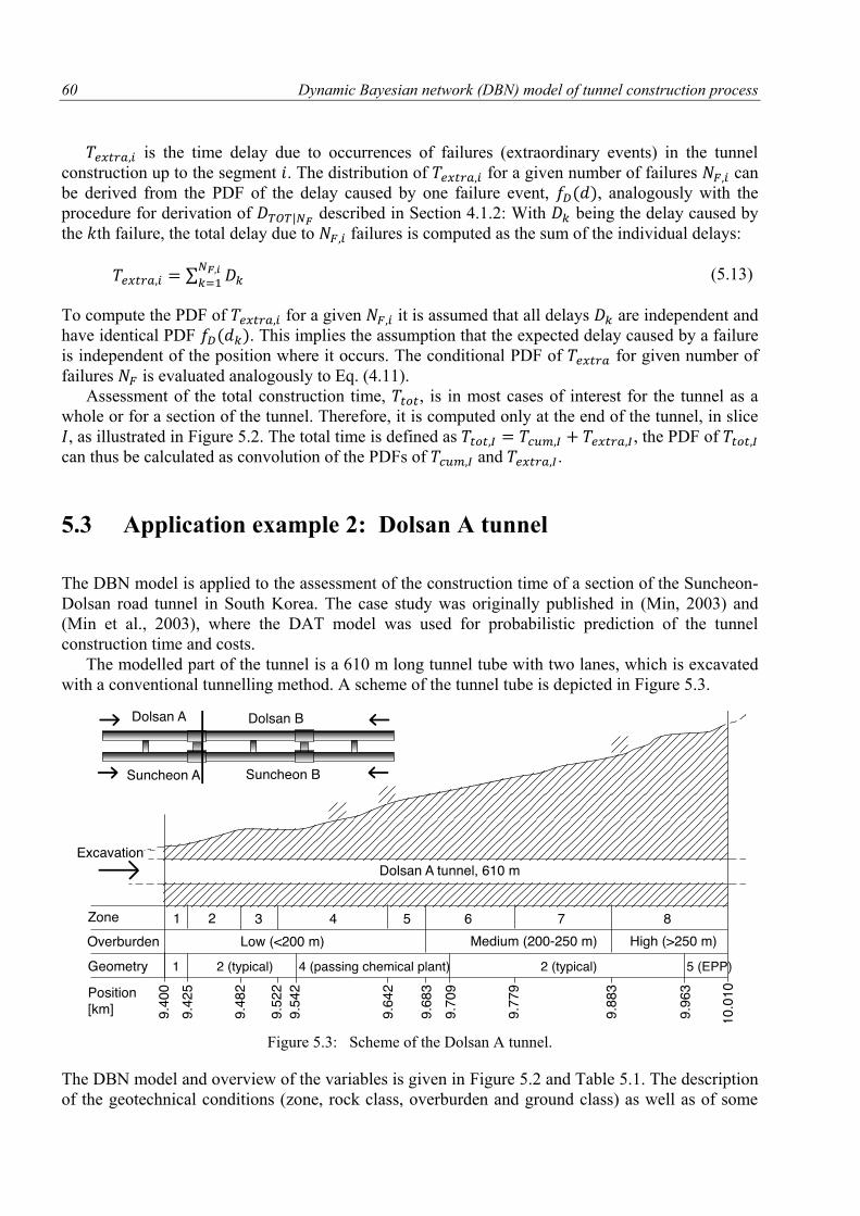
60 Dynamic Bayesian network (DBN) model of tunnel construction process
is the time delay due to occurrences of failures (extraordinary events) in the tunnel
construction up to the segment . The distribution of for a given number of failures can
be derived from the PDF of the delay caused by one failure event, , analogously with the
procedure for derivation of | described in Section 4.1.2: With being the delay caused by
the th failure, the total delay due to failures is computed as the sum of the individual delays:
∑
(5.13)
To compute the PDF of for a given it is assumed that all delays are independent and
have identical PDF . This implies the assumption that the expected delay caused by a failure
is independent of the position where it occurs. The conditional PDF of for given number of
failures is evaluated analogously to Eq. (4.11).
Assessment of the total construction time, , is in most cases of interest for the tunnel as a
whole or for a section of the tunnel. Therefore, it is computed only at the end of the tunnel, in slice
, as illustrated in Figure 5.2. The total time is defined as , the PDF of
can thus be calculated as convolution of the PDFs of and .
5.3 Application example 2: Dolsan A tunnel
The DBN model is applied to the assessment of the construction time of a section of the Suncheon-
Dolsan road tunnel in South Korea. The case study was originally published in (Min, 2003) and
(Min et al., 2003), where the DAT model was used for probabilistic prediction of the tunnel
construction time and costs.
The modelled part of the tunnel is a 610 m long tunnel tube with two lanes, which is excavated
with a conventional tunnelling method. A scheme of the tunnel tube is depicted in Figure 5.3.
Figure 5.3: Scheme of the Dolsan A tunnel.
The DBN model and overview of the variables is given in Figure 5.2 and Table 5.1. The description
of the geotechnical conditions (zone, rock class, overburden and ground class) as well as of some
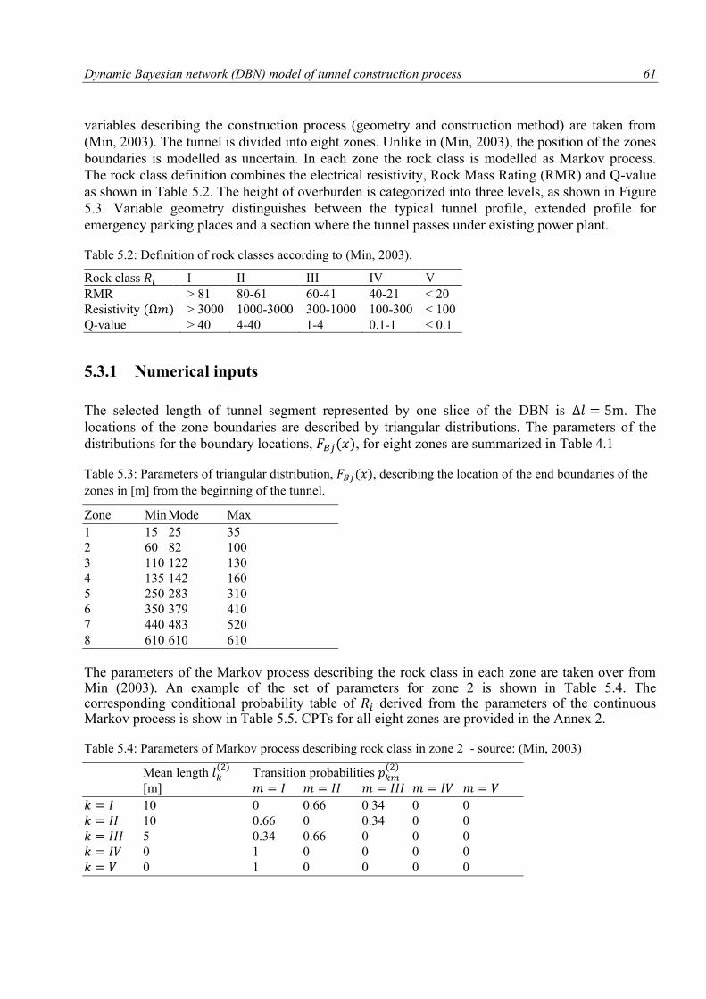
Dynamic Bayesian network (DBN) model of tunnel construction process 61
variables describing the construction process (geometry and construction method) are taken from
(Min, 2003). The tunnel is divided into eight zones. Unlike in (Min, 2003), the position of the zones
boundaries is modelled as uncertain. In each zone the rock class is modelled as Markov process.
The rock class definition combines the electrical resistivity, Rock Mass Rating (RMR) and Q-value
as shown in Table 5.2. The height of overburden is categorized into three levels, as shown in Figure
5.3. Variable geometry distinguishes between the typical tunnel profile, extended profile for
emergency parking places and a section where the tunnel passes under existing power plant.
Table 5.2: Definition of rock classes according to (Min, 2003).
Rock class I II III IV V
RMR > 81 80-61 60-41 40-21 < 20
Resistivity > 3000 1000-3000 300-1000 100-300 < 100
Q-value > 40 4-40 1-4 0.1-1 < 0.1
5.3.1 Numerical inputs
The selected length of tunnel segment represented by one slice of the DBN is . The
locations of the zone boundaries are described by triangular distributions. The parameters of the
distributions for the boundary locations, , for eight zones are summarized in Table 4.1
Table 5.3: Parameters of triangular distribution, , describing the location of the end boundaries of the
zones in [m] from the beginning of the tunnel.
Zone Min Mode Max
1 15 25 35
2 60 82 100
3 110 122 130
4 135 142 160
5 250 283 310
6 350 379 410
7 440 483 520
8 610 610 610
The parameters of the Markov process describing the rock class in each zone are taken over from Min (2003). An example of the set of parameters for zone 2 is shown in Table 5.4. The corresponding conditional probability table of derived from the parameters of the continuous Markov process is show in Table 5.5. CPTs for all eight zones are provided in the Annex 2.
Table 5.4: Parameters of Markov process describing rock class in zone 2 - source: (Min, 2003)
Mean length
Transition probabilities
[m]
10 0 0.66 0.34 0 0
10 0.66 0 0.34 0 0
5 0.34 0.66 0 0 0
0 1 0 0 0 0
0 1 0 0 0 0
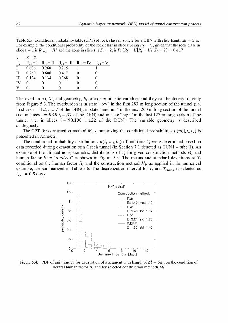
62 Dynamic Bayesian network (DBN) model of tunnel construction process
Table 5.5: Conditional probability table (CPT) of rock class in zone 2 for a DBN with slice length .
For example, the conditional probability of the rock class in slice being , given that the rock class in
slice is and the zone in slice is , is | .
v Zi = 2
Ri Ri-1 = I Ri-1 = II Ri-1 = III Ri-1 = IV Ri-1 = V
I 0.606 0.260 0.215 1 1
II 0.260 0.606 0.417 0 0
III 0.134 0.134 0.368 0 0
IV 0 0 0 0 0
V 0 0 0 0 0
The overburden, , and geometry, , are deterministic variables and they can be derived directly
from Figure 5.3. The overburden is in state “low” in the first 283 m long section of the tunnel (i.e.
in slices of the DBN), in state “medium” in the next 200 m long section of the tunnel
(i.e. in slices of the DBN) and in state “high” in the last 127 m long section of the
tunnel (i.e. in slices of the DBN). The variable geometry is described
analogously.
The CPT for construction method summarizing the conditional probabilities | is
presented in Annex 2.
The conditional probability distributions | of unit time were determined based on
data recorded during excavation of a Czech tunnel (in Section 7.1 denoted as TUN1 – tube 1). An
example of the utilized non-parametric distributions of for given construction methods and
human factor is shown in Figure 5.4. The means and standard deviations of
conditional on the human factor and the construction method , as applied in the numerical
example, are summarized in Table 5.6. The discretization interval for and is selected as
.
Figure 5.4: PDF of unit time for excavation of a segment with length of , on the condition of
neutral human factor and for selected construction methods
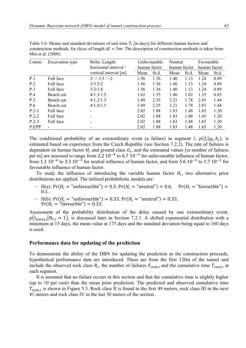
Dynamic Bayesian network (DBN) model of tunnel construction process 63
Table 5.6: Means and standard deviations of unit time [in days] for different human factors and
construction methods, for slices of length . The description of construction methods is taken from
Min et al. (2008).
Constr. Excavation type Bolts: Length/
horizontal interval /
vertical interval [m]
Unfavourable
human factor
Neutral
human factor
Favourable
human factor
Mean St.d. Mean St.d. Mean St.d.
P.1 Full face 3/ > 3.5 / >2 1.56 1.36 1.40 1.13 1.24 0.89
P.2 Full face 3/3.5/2 1.56 1.36 1.40 1.13 1.24 0.89
P.3 Full face 3/2/1.8 1.56 1.36 1.40 1.13 1.24 0.89
P.4 Bench cut 4/1.5/1.5 1.62 1.35 1.46 1.02 1.35 0.83
P.5 Bench cut 4/1.2/1.5 3.49 2.35 3.21 1.78 2.83 1.44
P.6 Bench cut 4/1.0/1.5 3.49 2.35 3.21 1.78 2.83 1.44
P.2-1 Full face - 2.02 1.88 1.83 1.48 1.65 1.20
P.2-2 Full face - 2.02 1.88 1.83 1.48 1.65 1.20
P.2-3 Full face - 2.02 1.88 1.83 1.48 1.65 1.20
P.EPP - - 2.02 1.88 1.83 1.48 1.65 1.20
The conditional probability of an extraordinary event (a failure) in segment , | , is
estimated based on experience from the Czech Republic (see Section 7.2.2). The rate of failures is
dependent on human factor and ground class , and the estimated values [in number of failures
per m] are assessed to range from to for unfavourable influence of human factor,
from to for neutral influence of human factor, and from to for
favourable influence of human factor.
To study the influence of introducing the variable human factor , two alternative prior
distributions are applied. The utilized probabilistic models are:
H(a): , , .
H(b): , , .
Assessment of the probability distribution of the delay caused by one extraordinary event,
( | ), is discussed later in Section 7.2.1. A shifted exponential distribution with a
minimum at 15 days, the mean value at 175 days and the standard deviation being equal to 160 days
is used.
Performance data for updating of the prediction
To demonstrate the ability of the DBN for updating the prediction as the construction proceeds,
hypothetical performance data are introduced. These are from the first 120m of the tunnel and
include the observed rock class , the number of failures and the cumulative time at
each segment.
It is assumed that no failure occurs in this section and that the cumulative time is slightly higher
(up to 10 per cent) than the mean prior prediction. The predicted and observed cumulative time
is shown in Figure 5.5. Rock class II is found in the first 49 meters, rock class III in the next
41 meters and rock class IV in the last 30 meters of the section.
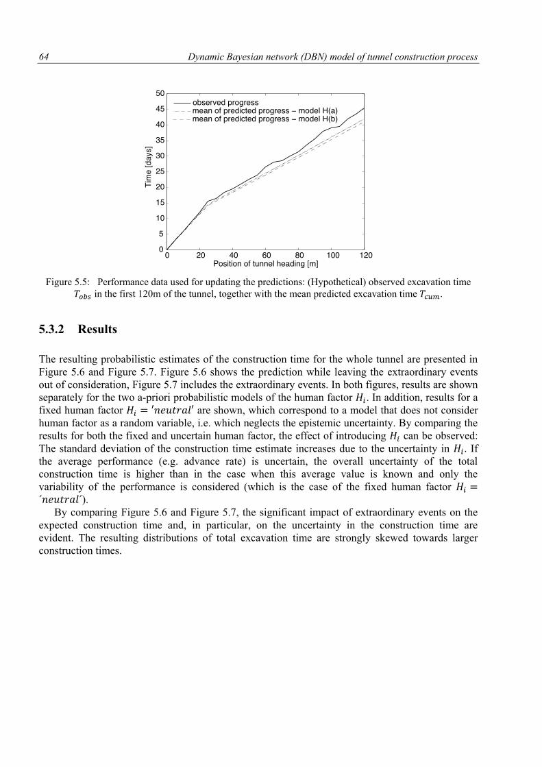
64 Dynamic Bayesian network (DBN) model of tunnel construction process
Figure 5.5: Performance data used for updating the predictions: (Hypothetical) observed excavation time
in the first 120m of the tunnel, together with the mean predicted excavation time .
5.3.2 Results
The resulting probabilistic estimates of the construction time for the whole tunnel are presented in
Figure 5.6 and Figure 5.7. Figure 5.6 shows the prediction while leaving the extraordinary events
out of consideration, Figure 5.7 includes the extraordinary events. In both figures, results are shown
separately for the two a-priori probabilistic models of the human factor . In addition, results for a
fixed human factor are shown, which correspond to a model that does not consider
human factor as a random variable, i.e. which neglects the epistemic uncertainty. By comparing the
results for both the fixed and uncertain human factor, the effect of introducing can be observed:
The standard deviation of the construction time estimate increases due to the uncertainty in . If
the average performance (e.g. advance rate) is uncertain, the overall uncertainty of the total
construction time is higher than in the case when this average value is known and only the
variability of the performance is considered (which is the case of the fixed human factor ).
By comparing Figure 5.6 and Figure 5.7, the significant impact of extraordinary events on the
expected construction time and, in particular, on the uncertainty in the construction time are
evident. The resulting distributions of total excavation time are strongly skewed towards larger
construction times.
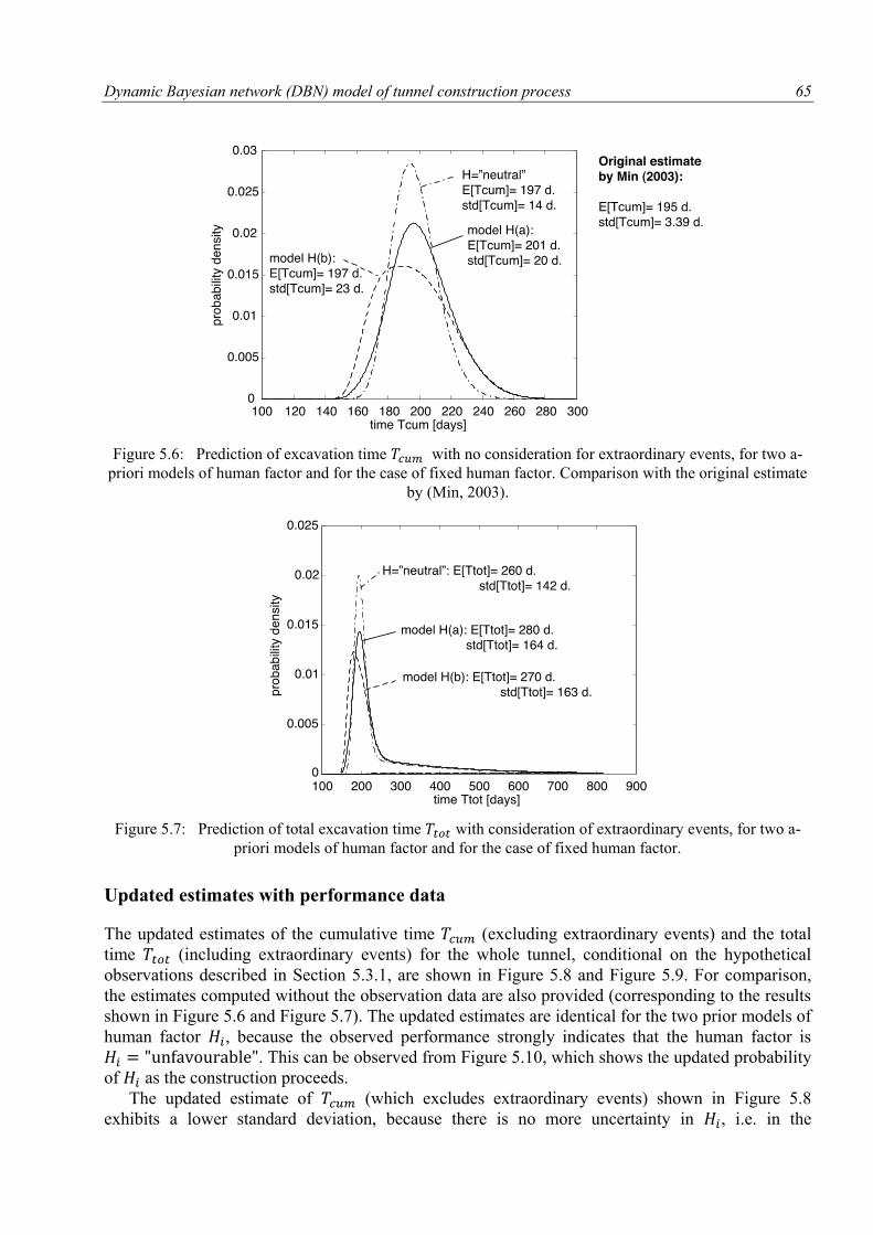
Dynamic Bayesian network (DBN) model of tunnel construction process 65
Figure 5.6: Prediction of excavation time with no consideration for extraordinary events, for two a-
priori models of human factor and for the case of fixed human factor. Comparison with the original estimate
by (Min, 2003).
Figure 5.7: Prediction of total excavation time with consideration of extraordinary events, for two a-
priori models of human factor and for the case of fixed human factor.
Updated estimates with performance data
The updated estimates of the cumulative time (excluding extraordinary events) and the total
time (including extraordinary events) for the whole tunnel, conditional on the hypothetical
observations described in Section 5.3.1, are shown in Figure 5.8 and Figure 5.9. For comparison,
the estimates computed without the observation data are also provided (corresponding to the results
shown in Figure 5.6 and Figure 5.7). The updated estimates are identical for the two prior models of
human factor , because the observed performance strongly indicates that the human factor is
. This can be observed from Figure 5.10, which shows the updated probability
of as the construction proceeds.
The updated estimate of (which excludes extraordinary events) shown in Figure 5.8
exhibits a lower standard deviation, because there is no more uncertainty in , i.e. in the
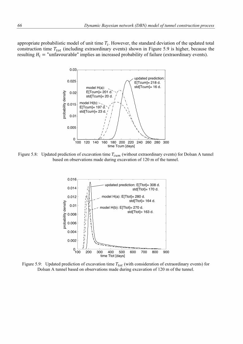
66 Dynamic Bayesian network (DBN) model of tunnel construction process
appropriate probabilistic model of unit time . However, the standard deviation of the updated total
construction time (including extraordinary events) shown in Figure 5.9 is higher, because the
resulting implies an increased probability of failure (extraordinary events).
Figure 5.8: Updated prediction of excavation time (without extraordinary events) for Dolsan A tunnel
based on observations made during excavation of 120 m of the tunnel.
Figure 5.9: Updated prediction of excavation time (with consideration of extraordinary events) for
Dolsan A tunnel based on observations made during excavation of 120 m of the tunnel.
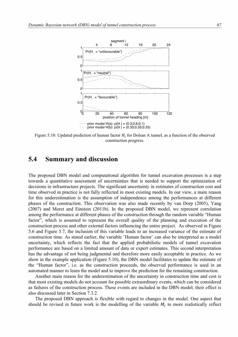
Dynamic Bayesian network (DBN) model of tunnel construction process 67
Figure 5.10: Updated prediction of human factor for Dolsan A tunnel, as a function of the observed
construction progress.
5.4 Summary and discussion
The proposed DBN model and computational algorithm for tunnel excavation processes is a step
towards a quantitative assessment of uncertainties that is needed to support the optimization of
decisions in infrastructure projects. The significant uncertainty in estimates of construction cost and
time observed in practice is not fully reflected in most existing models. In our view, a main reason
for this underestimation is the assumption of independence among the performances at different
phases of the construction. This observation was also made recently by van Dorp (2005), Yang
(2007) and Moret and Einstein (2011b). In the proposed DBN model, we represent correlation
among the performance at different phases of the construction through the random variable “Human
factor”, which is assumed to represent the overall quality of the planning and execution of the
construction process and other external factors influencing the entire project. As observed in Figure
5.6 and Figure 5.7, the inclusion of this variable leads to an increased variance of the estimate of
construction time. As stated earlier, the variable ¨Human factor¨ can also be interpreted as a model
uncertainty, which reflects the fact that the applied probabilistic models of tunnel excavation
performance are based on a limited amount of data or expert estimates. This second interpretation
has the advantage of not being judgmental and therefore more easily acceptable in practice. As we
show in the example application (Figure 5.10), the DBN model facilitates to update the estimate of
the “Human factor”, i.e. as the construction proceeds, the observed performance is used in an
automated manner to learn the model and to improve the prediction for the remaining construction.
Another main reason for the underestimation of the uncertainty in construction time and cost is
that most existing models do not account for possible extraordinary events, which can be considered
as failures of the construction process. These events are included in the DBN model; their effect is
also discussed later in Section 7.3.2.
The proposed DBN approach is flexible with regard to changes in the model. One aspect that
should be revised in future work is the modelling of the variable to more realistically reflect

68 Dynamic Bayesian network (DBN) model of tunnel construction process
changes of construction technology during the excavation process. The present model assumes full
flexibility in changing the construction patterns based on changes in geology. In reality, the
construction pattern is not modified so frequently, as this is connected with additional time and
costs. This effect is even more pronounced when mechanized excavation is used. A second aspect
that should be addressed is the modelling of costs. The variable time can be replaced by the variable
cost to obtain a cost estimate. However, for a combined modelling, an extension of the DBN model
is needed to account for the dependence of construction costs on construction time.
The DBN is computationally efficient and applicable in practice. It is flexible in including
observations to update the predictions. Besides updating the model with performance data and the
observed geology of the excavated tunnel sections, as shown in Section 5.3, other types of
observations, e.g. borehole tests, can be included in the future.
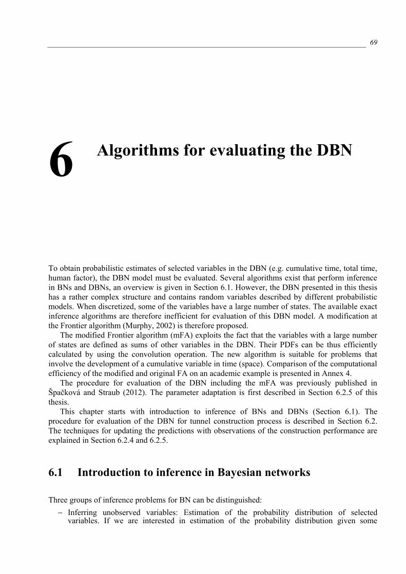
69
To obtain probabilistic estimates of selected variables in the DBN (e.g. cumulative time, total time,
human factor), the DBN model must be evaluated. Several algorithms exist that perform inference
in BNs and DBNs, an overview is given in Section 6.1. However, the DBN presented in this thesis
has a rather complex structure and contains random variables described by different probabilistic
models. When discretized, some of the variables have a large number of states. The available exact
inference algorithms are therefore inefficient for evaluation of this DBN model. A modification at
the Frontier algorithm (Murphy, 2002) is therefore proposed.
The modified Frontier algorithm (mFA) exploits the fact that the variables with a large number
of states are defined as sums of other variables in the DBN. Their PDFs can be thus efficiently
calculated by using the convolution operation. The new algorithm is suitable for problems that
involve the development of a cumulative variable in time (space). Comparison of the computational
efficiency of the modified and original FA on an academic example is presented in Annex 4.
The procedure for evaluation of the DBN including the mFA was previously published in
Špačková and Straub (2012). The parameter adaptation is first described in Section 6.2.5 of this
thesis.
This chapter starts with introduction to inference of BNs and DBNs (Section 6.1). The
procedure for evaluation of the DBN for tunnel construction process is described in Section 6.2.
The techniques for updating the predictions with observations of the construction performance are
explained in Section 6.2.4 and 6.2.5.
6.1 Introduction to inference in Bayesian networks
Three groups of inference problems for BN can be distinguished:
Inferring unobserved variables: Estimation of the probability distribution of selected variables. If we are interested in estimation of the probability distribution given some
6 Algorithms for evaluating the DBN
70 Algorithms for evaluating the DBN
observations (also called evidence in the BN terminology), we speak about updating of the original estimate.
Parameter learning: Determination of the conditional probabilities (CPT tables) from data. The CPT tables can also be updated with observed data; this procedure is called adaptation of the parameters.
Structure learning: Determination of the structure of the Bayesian network from data. This type of inference is not used in this thesis and is thus not discussed in more detail.
Several algorithms exist for solving these inference problems; they are either exact or approximate
algorithms. Selection of the appropriate algorithm depends on the complexity of the network and on
the probability distributions of the variables included in the network. Generally, the computational
effort increases exponentially with the number of nodes and links in the BN and with the number of
states of discrete variables.
Many software packages can be used for building and evaluating the BNs. These are for
example freeware codes such as Genie developed at the University of Pittsburg
(http://genie.sis.pitt.edu/), Elvira developed at the university of Granada (http://leo.ugr.es/elvira/) or
commercial products such as Hugin (http://www.hugin.com/), Agena (http://www.agenarisk.com/)
and Netica (http://www.norsys.com). An overview of the software solutions is available at
http://www.cs.ubc.ca/~murphyk/Bayes/bnsoft.html. A Bayesian network toolbox for Matlab has
been developed by Kevin Murphy and is freely available (http://code.google.com/p/bnt/). However,
for more complex problems and where changes of the existing algorithms are required, utilization
of the available software is impractical. The algorithm presented in Section 6.2 is therefore
implemented in Matlab environment with its statistical toolbox.
6.1.1 Inferring unobserved variables
First we limit ourselves to BNs with discrete RVs. The same example BN which is presented in the
Section 3.3.5 is used for illustration. The BN is also displayed in Figure 6.1(a).
The first basic operation used in evaluating the BNs is the combination of probability
distributions. This operation is used for calculating the joint PMF of selected set of RVs (Langseth
et al., 2009). It corresponds to the application of the chain rule. For the example BN it is illustrated
in Eq. (3.10) and it is repeated here:
| | | (6.1)
The second basic procedure is the elimination of variables (also called marginalization in the BN
terminology), which corresponds to removing selected RVs from the joint PMF. Because the states
of the discrete random variables are mutually exclusive and collectively exhausting events,
elimination of a variable corresponds to summing a joint PMF containing the variable over all states
of the variable.
To eliminate the variable from the joint PMF describing the whole BN, the following
calculation is performed:
∑ (6.2)
where the notation ∑ denotes the summation over all states of . The elimination operation can
be performed repeatedly for selected variables at any stage of the calculations; in this way, the
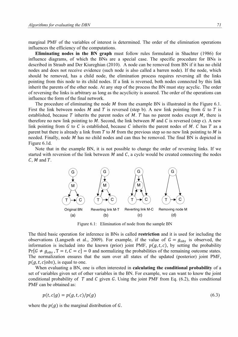
Algorithms for evaluating the DBN 71
marginal PMF of the variables of interest is determined. The order of the elimination operations
influences the efficiency of the computations.
Eliminating nodes in the BN graph must follow rules formulated in Shachter (1986) for
influence diagrams, of which the BNs are a special case. The specific procedure for BNs is
described in Straub and Der Kiureghian (2010). A node can be removed from BN if it has no child
nodes and does not receive evidence (such node is also called a barren node). If the node, which
should be removed, has a child node, the elimination process requires reversing all the links
pointing from this node to its child nodes. If a link is reversed, both nodes connected by this link
inherit the parents of the other node. At any step of the process the BN must stay acyclic. The order
of reversing the links is arbitrary as long as the acyclicity is assured. The order of the operations can
influence the form of the final network.
The procedure of eliminating the node from the example BN is illustrated in the Figure 6.1.
First the link between nodes and is reversed (step b). A new link pointing from to is
established, because inherits the parent nodes of . has no parent nodes except , there is
therefore no new link pointing to . Second, the link between and is reversed (step c). A new
link pointing from to is established, because inherits the parent nodes of . has as a
parent but there is already a link from to from the previous step so no new link pointing to is
needed. Finally, node has no child nodes and can thus be removed. The final BN is depicted in
Figure 6.1d.
Note that in the example BN, it is not possible to change the order of reversing links. If we
started with reversion of the link between and , a cycle would be created connecting the nodes
, and .
Figure 6.1: Elimination of node from the sample BN
The third basic operation for inference in BNs is called restriction and it is used for including the
observations (Langseth et al., 2009). For example, if the value of is observed, the
information is included into the known (prior) joint PMF, , by setting the probability
[ ] and normalizing the probabilities of the remaining outcome states.
The normalization ensures that the sum over all states of the updated (posterior) joint PMF,
| , is equal to one.
When evaluating a BN, one is often interested in calculating the conditional probability of a
set of variables given set of other variables in the BN. For example, we can want to know the joint
conditional probability of and given Using the joint PMF from Eq. (6.2), this conditional
PMF can be obtained as:
| (6.3)
where the is the marginal distribution of
72 Algorithms for evaluating the DBN
In real problems it is not efficient to calculate the full joint PMF of all variables in the BN.
Therefore, it is necessary to find a sequence of operations (combination of PMFs, elimination of
nodes, restriction and calculation of conditional probabilities), which gives the required answer and
at the same time is computationally efficient. The exact inference algorithms for BNs generally
aim to find such an optimal sequence of operations using the graph theory or other techniques. The
universally used ones are the junction trees and joint trees (Jensen and Nielsen, 2007). The exact
inference algorithms require the RVs in the network to be discrete.
As evident from the previous description, a principal computational task in evaluating the BNs
is the numerical integration of the joint probability functions (resp. their summation in the discrete
space). The approximate inference algorithms are mostly using various sampling methods
(nondeterministic methods) or deterministic methods to perform such integration (Minka, 2001).
Only a brief overview of the approximate methods is given here, because they are not further used
for evaluation of the proposed DBN.
The commonly used sampling (nondeterministic) methods are for example Markov Chain
Monte Carlo (MCMC) simulation (Gilks et al., 1996), importance sampling (Yuan and Druzdzel,
2006), likelihood weighting or rejection sampling (Russell and Norvig, 2003). The main advantage
of the sampling methods is their flexibility; they can be applied to any BN as they are not limited by
the type of RVs in the network. The main disadvantage is their computational inefficiency.
The approximate methods using deterministic methods generally aim to approximate the
required integrand, i.e. the (joint) PMF of required set of RVs. These are for example the
Variational methods, Loopy belief propagation, Bayesian averaging, Laplace’s method or
Expectation propagation. These methods can be computationally very efficient but their application
is limited by several restrictions, which the evaluated BN must fulfill. Additionally, they often
strongly simplify the results e.g. when assuming them to be Gaussian. For a detailed discussion on
these methods, the reader is referred to Minka (2001) and Murphy (2002).
BNs with continuous RVs
A BN can consist of continuous RVs (then it is called a continuous BN) or it can combine both the
discrete and continuous RVs (then it is called a hybrid BN).
BNs with Gaussian variables or hybrid BNs with discrete and conditionally Gaussian variables
have been studied extensively and efficient algorithms for their evaluation are available. They
utilize the fact that under a linear dependence structure the joint probability function of Gaussian
variables is also Gaussian. An example hybrid BN with conditionally Gaussian RVs is presented in
Annex 4.
The joint probability functions of non-Gaussian variables are not defined. Therefore, evaluation
of the BNs containing continuous non-Gaussian RVs requires utilization of approximate algorithms
or discretization of the RVs. When the RVs are discretized, the previously discussed exact
algorithms can be applied. The discretization process is described later in Section 6.1.3.
In hybrid BNs, where we are not interested in the probability distribution of the continuous RVs,
these can be eliminated from the BN and the resulting BN can be solved by the known exact
inference algorithm as proposed in Straub and Der Kiureghian (2010).
Inference in DBNs
The algorithms for evaluating DBNs are based on the same principles that apply to inference in the
BNs. Because the DBN consist of repeating sets of nodes, the inference algorithms have a
Algorithms for evaluating the DBN 73
recursive nature. They generally involve the so-called forward and backward passes: The forward
pass evaluates the DBN slice by slice from the beginning (i.e. from left to right) and the backward
pass from its end (i.e. from right to left).
In most cases, only some of the RVs are observable. Let denote the observed RVs in slice and denote the unobserved (hidden) RVs in slice . Three types of tasks can be distinguished
(Murphy, 2002):
Filtering: Estimating the state of the system in time/position , having observations from slices . It corresponds to evaluating the probability | and requires application of the forward pass up to the slice .
Prediction: Estimating a future state of the system in time/position , where , knowing the observations from slices . It corresponds to evaluating the probability | and requires application of the forward pass up to the slice ; in slices no evidence is included.
Smoothing: Estimating a past state of the system in the th slice of the DBN, where , knowing the observations from slices . It corresponds to evaluating the probability | and requires application of both the forward and backward pass. This case is not further discussed in this thesis.
From these three operations, we only perform prediction in this thesis, either with or without
evidence.
The exact algorithms for DBNs with discrete RVs are the Frontier algorithm, which is in more
detail discussed later in Section 6.1.3, or the Interface algorithm, which is a modification of the
Frontier algorithm optimizing the set of nodes operated at each step of the evaluation suggested by
(Murphy, 2002). A complex summary of the algorithms for DBNs is provided in Murphy (2002) or
Russell and Norvig (2003).
6.1.2 Parameter learning
Two problems are solved when learning the BN parameters from data:
Prior estimation of the model parameters (also called off-line learning), where a large set of data is available at once.
Sequential updating/adaptation of the parameters with observations (also called on-line learning), where model parameters are updated with every new set of observations.
Different methods must be used for complete and incomplete data sets. Only the methods used later
in the thesis are introduced in more detail in this section. Techniques for learning parameters of
BNs are also applicable for DBNs (Murphy, 2002).
We assume that the structure of the BN is known and that the parameters for the various RVs in
the network are independent, i.e. that we can learn the parameters of each RV independently. Let
be the set parameters of the analyzed variable , be the best estimate of the parameters and be
the data set. If the random variable is discrete, consists of the values in the CPT. If the RV is
continuous and it is described by a parametric distribution (e.g. Normal, Lognormal etc.)
conditionally on its parents, contains the parameters of the parametric probability distribution.
74 Algorithms for evaluating the DBN
Prior estimation
The most common approach to the prior estimate of the BN parameters with a complete data set is
the Maximum likelihood estimation (MLE), which aims to maximize the likelihood (resp. log-
likelihood) of the parameter set given the observed data set :
| | (6.4)
The likelihood is calculated as
| ∏ [ | ] (6.5)
where is a single observation of the variable . For computational reasons it is more convenient
to work with log-likelihood, which is defined as:
| ∑ [ | ] (6.6)
Note that Eqs. (6.4) - (6.6) assume independence of observations for given .
If the dataset is not large enough, we may wish to combine the data with experience. In this
case, the Bayesian approach is suitable allowing one to combine a prior estimate of the
parameters, obtained for example from an older database, literature or expert judgment, with new
data. This technique is not used in this thesis, for more details the reader is referred for example to
Russell and Norvig (2003) or Špačková et al. (2011).
The Expectation maximization (EM) algorithm is a popular method for learning parameters
from an incomplete dataset. It is used when data in the dataset are missing or some variables are not
observable (Jensen and Nielsen, 2007). It is an iterative approach consisting of two steps: in the
expectation step, the missing data are replaced with expected values obtained based on the current
estimate of parameters; in the maximization step, the new set of data is used to make new parameter
estimate.
Please note that in the example of Section 5.3, we also deal with incomplete data, because the
variable human factor is not observed. However, for learning the model parameters we make
assumption on the state of the unobserved variable (we assume it to be in the state “neutral”).
Therefore, the MLE algorithm is used for learning the parameters of unit time.
Updating/adaptation of the parameters
The (epistemic) uncertainty in the model parameters can be conveniently modelled by introducing
an unobservable model type variable into the BN (Jensen and Nielsen, 2007;Der Kiureghian and
Ditlevsen, 2009). This hidden variable is automatically updated with observations using the
inference methods described in Section 6.1.1. In the DBN model of the tunnel construction process,
the variable is such a hidden variable. If this type of updating is not sufficient, the parameters of
the BN (i.e. the CPTs) can be updated directly by means of Fractional updating or Fading (Jensen
and Nielsen, 2007). Both methods are approximate, the Fractional updating is described in more
detail in the following:
We want to update the CPT of variable , which is defined conditionally on variables and .
Let [ | ] be the prior estimate of the parameter and
[ | ] be the updated estimate. The reliability of the prior
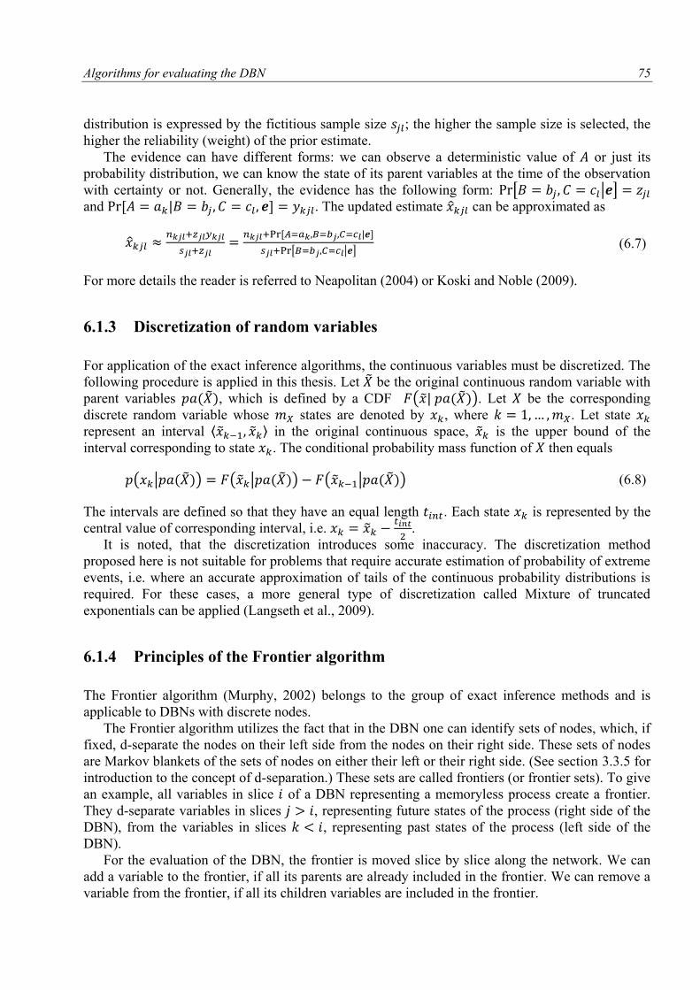
Algorithms for evaluating the DBN 75
distribution is expressed by the fictitious sample size ; the higher the sample size is selected, the
higher the reliability (weight) of the prior estimate.
The evidence can have different forms: we can observe a deterministic value of or just its
probability distribution, we can know the state of its parent variables at the time of the observation
with certainty or not. Generally, the evidence has the following form: [ | ] and [ | ] . The updated estimate can be approximated as
[ | ]
[ | ] (6.7)
For more details the reader is referred to Neapolitan (2004) or Koski and Noble (2009).
6.1.3 Discretization of random variables
For application of the exact inference algorithms, the continuous variables must be discretized. The
following procedure is applied in this thesis. Let be the original continuous random variable with
parent variables , which is defined by a CDF ( | ). Let be the corresponding
discrete random variable whose states are denoted by , where . Let state
represent an interval ⟨ ⟩ in the original continuous space, is the upper bound of the
interval corresponding to state . The conditional probability mass function of then equals
( | ) ( | ) ( | ) (6.8)
The intervals are defined so that they have an equal length . Each state is represented by the
central value of corresponding interval, i.e.
.
It is noted, that the discretization introduces some inaccuracy. The discretization method
proposed here is not suitable for problems that require accurate estimation of probability of extreme
events, i.e. where an accurate approximation of tails of the continuous probability distributions is
required. For these cases, a more general type of discretization called Mixture of truncated
exponentials can be applied (Langseth et al., 2009).
6.1.4 Principles of the Frontier algorithm
The Frontier algorithm (Murphy, 2002) belongs to the group of exact inference methods and is
applicable to DBNs with discrete nodes.
The Frontier algorithm utilizes the fact that in the DBN one can identify sets of nodes, which, if
fixed, d-separate the nodes on their left side from the nodes on their right side. These sets of nodes
are Markov blankets of the sets of nodes on either their left or their right side. (See section 3.3.5 for
introduction to the concept of d-separation.) These sets are called frontiers (or frontier sets). To give
an example, all variables in slice of a DBN representing a memoryless process create a frontier.
They d-separate variables in slices , representing future states of the process (right side of the
DBN), from the variables in slices , representing past states of the process (left side of the
DBN).
For the evaluation of the DBN, the frontier is moved slice by slice along the network. We can
add a variable to the frontier, if all its parents are already included in the frontier. We can remove a
variable from the frontier, if all its children variables are included in the frontier.
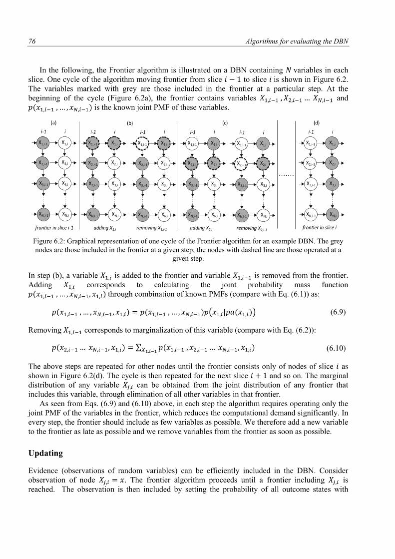
76 Algorithms for evaluating the DBN
In the following, the Frontier algorithm is illustrated on a DBN containing variables in each
slice. One cycle of the algorithm moving frontier from slice to slice is shown in Figure 6.2.
The variables marked with grey are those included in the frontier at a particular step. At the
beginning of the cycle (Figure 6.2a), the frontier contains variables and
is the known joint PMF of these variables.
Figure 6.2: Graphical representation of one cycle of the Frontier algorithm for an example DBN. The grey
nodes are those included in the frontier at a given step; the nodes with dashed line are those operated at a
given step.
In step (b), a variable is added to the frontier and variable is removed from the frontier.
Adding corresponds to calculating the joint probability mass function
through combination of known PMFs (compare with Eq. (6.1)) as:
( | ) (6.9)
Removing corresponds to marginalization of this variable (compare with Eq. (6.2)):
∑ (6.10)
The above steps are repeated for other nodes until the frontier consists only of nodes of slice as
shown in Figure 6.2(d). The cycle is then repeated for the next slice and so on. The marginal
distribution of any variable can be obtained from the joint distribution of any frontier that
includes this variable, through elimination of all other variables in that frontier.
As seen from Eqs. (6.9) and (6.10) above, in each step the algorithm requires operating only the
joint PMF of the variables in the frontier, which reduces the computational demand significantly. In
every step, the frontier should include as few variables as possible. We therefore add a new variable
to the frontier as late as possible and we remove variables from the frontier as soon as possible.
Updating
Evidence (observations of random variables) can be efficiently included in the DBN. Consider
observation of node . The frontier algorithm proceeds until a frontier including is
reached. The observation is then included by setting the probability of all outcome states with
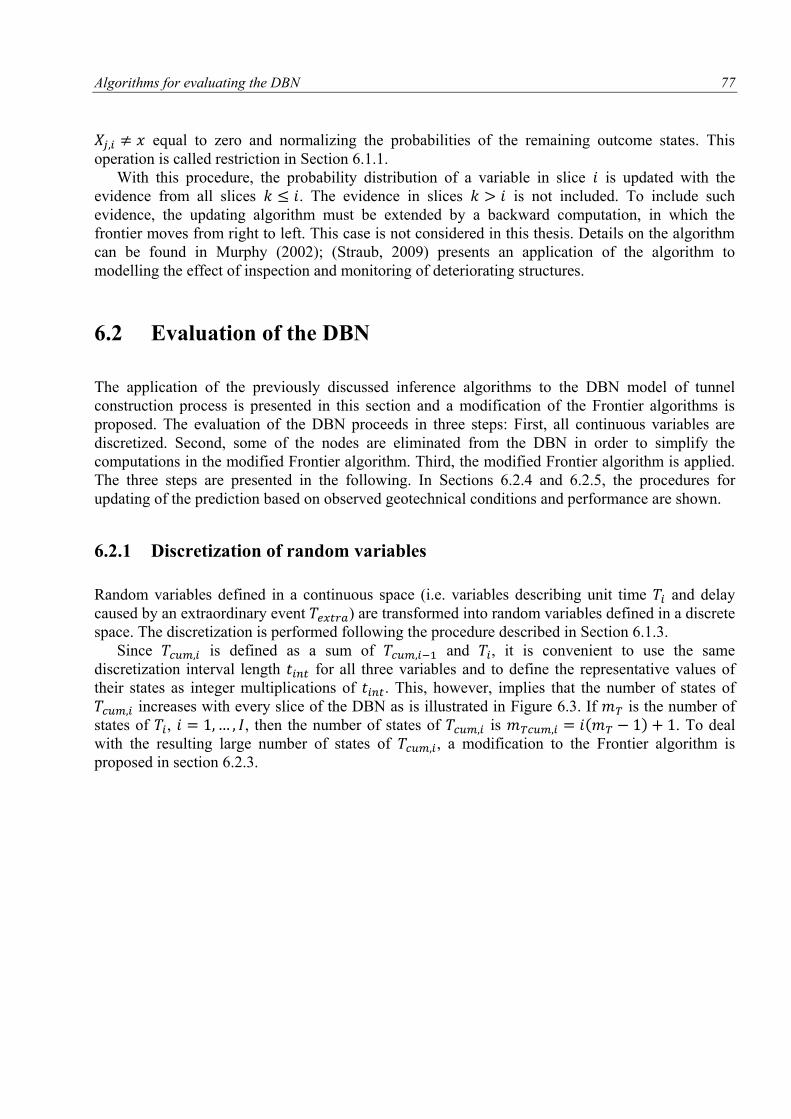
Algorithms for evaluating the DBN 77
equal to zero and normalizing the probabilities of the remaining outcome states. This
operation is called restriction in Section 6.1.1.
With this procedure, the probability distribution of a variable in slice is updated with the
evidence from all slices . The evidence in slices is not included. To include such
evidence, the updating algorithm must be extended by a backward computation, in which the
frontier moves from right to left. This case is not considered in this thesis. Details on the algorithm
can be found in Murphy (2002); (Straub, 2009) presents an application of the algorithm to
modelling the effect of inspection and monitoring of deteriorating structures.
6.2 Evaluation of the DBN
The application of the previously discussed inference algorithms to the DBN model of tunnel
construction process is presented in this section and a modification of the Frontier algorithms is
proposed. The evaluation of the DBN proceeds in three steps: First, all continuous variables are
discretized. Second, some of the nodes are eliminated from the DBN in order to simplify the
computations in the modified Frontier algorithm. Third, the modified Frontier algorithm is applied.
The three steps are presented in the following. In Sections 6.2.4 and 6.2.5, the procedures for
updating of the prediction based on observed geotechnical conditions and performance are shown.
6.2.1 Discretization of random variables
Random variables defined in a continuous space (i.e. variables describing unit time and delay
caused by an extraordinary event ) are transformed into random variables defined in a discrete
space. The discretization is performed following the procedure described in Section 6.1.3.
Since is defined as a sum of and , it is convenient to use the same
discretization interval length for all three variables and to define the representative values of
their states as integer multiplications of . This, however, implies that the number of states of
increases with every slice of the DBN as is illustrated in Figure 6.3. If is the number of
states of , , then the number of states of is . To deal
with the resulting large number of states of , a modification to the Frontier algorithm is
proposed in section 6.2.3.
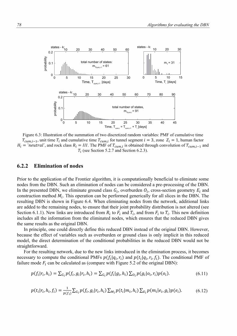
78 Algorithms for evaluating the DBN
Figure 6.3: Illustration of the summation of two discretized random variables: PMF of cumulative time
, unit time and cumulative time for tunnel segment , zone , human factor
, and rock class . The PMF of is obtained through convolution of and
(see Section 5.2.7 and Section 6.2.3).
6.2.2 Elimination of nodes
Prior to the application of the Frontier algorithm, it is computationally beneficial to eliminate some
nodes from the DBN. Such an elimination of nodes can be considered a pre-processing of the DBN.
In the presented DBN, we eliminate ground class , overburden , cross-section geometry and
construction method . This operation can be performed generically for all slices in the DBN. The
resulting DBN is shown in Figure 6.4. When eliminating nodes from the network, additional links
are added to the remaining nodes, to ensure that their joint probability distribution is not altered (see
Section 6.1.1). New links are introduced from to and , and from to . This new definition
includes all the information from the eliminated nodes, which ensures that the reduced DBN gives
the same results as the original DBN.
In principle, one could directly define this reduced DBN instead of the original DBN. However,
because the effect of variables such as overburden or ground class is only implicit in this reduced
model, the direct determination of the conditional probabilities in the reduced DBN would not be
straightforward.
For the resulting network, due to the new links introduced in the elimination process, it becomes
necessary to compute the conditional PMFs | and | . The conditional PMF of
failure mode can be calculated as (compare with Figure 5.2 of the original DBN):
| ∑ | ∑ | ∑ |
(6.11)
|
∑ | ∑ | ∑ |
(6.12)
0 5 10 15 20 25 30 35 40 450
0.1
0.210 20 30 40 50 60 70 80 90
0 5 10 15
10 20 30
0 5 10 15 20 25 30
10 20 30 40 50 60states - k:
total number of states,
mTcum,i
= 91
states - k:
mT = 31
pro
babili
ty
0
0.1
0.2
pro
babili
ty
Time, Tcum,i-1
[days] Time, Ti [days]
Time, Tcum,i
= Tcum,i-1
+ Ti [days]
states - k:
total number of states:
mTcum,i-1
= 61
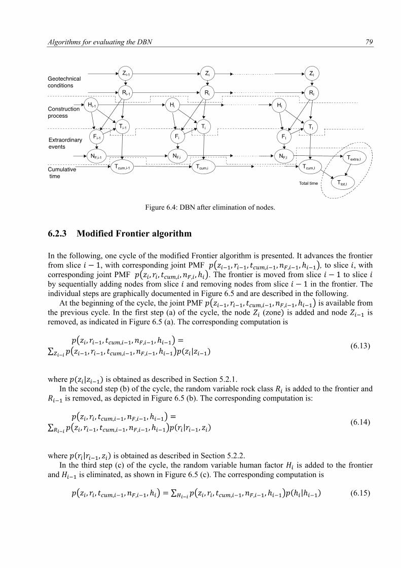
Algorithms for evaluating the DBN 79
Figure 6.4: DBN after elimination of nodes.
6.2.3 Modified Frontier algorithm
In the following, one cycle of the modified Frontier algorithm is presented. It advances the frontier
from slice , with corresponding joint PMF ( ), to slice , with
corresponding joint PMF ( ). The frontier is moved from slice to slice by sequentially adding nodes from slice and removing nodes from slice in the frontier. The
individual steps are graphically documented in Figure 6.5 and are described in the following.
At the beginning of the cycle, the joint PMF ( ) is available from
the previous cycle. In the first step (a) of the cycle, the node (zone is added and node is
removed, as indicated in Figure 6.5 (a). The corresponding computation is
( )
∑ ( ) |
(6.13)
where | is obtained as described in Section 5.2.1.
In the second step (b) of the cycle, the random variable rock class is added to the frontier and
is removed, as depicted in Figure 6.5 (b). The corresponding computation is:
( )
∑ ( ) |
(6.14)
where | is obtained as described in Section 5.2.2.
In the third step (c) of the cycle, the random variable human factor is added to the frontier
and is eliminated, as shown in Figure 6.5 (c). The corresponding computation is
( ) ∑ ( ) | (6.15)
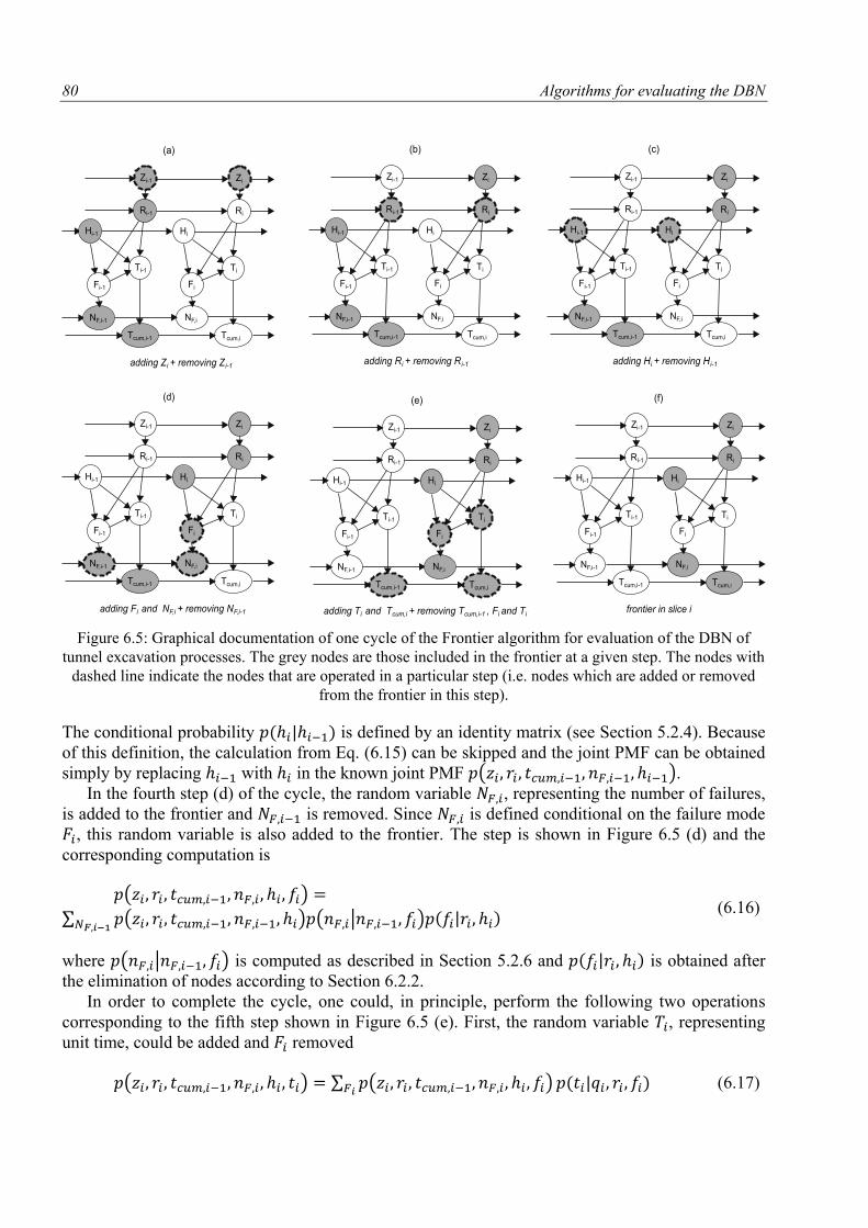
80 Algorithms for evaluating the DBN
Figure 6.5: Graphical documentation of one cycle of the Frontier algorithm for evaluation of the DBN of
tunnel excavation processes. The grey nodes are those included in the frontier at a given step. The nodes with
dashed line indicate the nodes that are operated in a particular step (i.e. nodes which are added or removed
from the frontier in this step).
The conditional probability | is defined by an identity matrix (see Section 5.2.4). Because
of this definition, the calculation from Eq. (6.15) can be skipped and the joint PMF can be obtained
simply by replacing with in the known joint PMF ( ).
In the fourth step (d) of the cycle, the random variable , representing the number of failures,
is added to the frontier and is removed. Since is defined conditional on the failure mode
, this random variable is also added to the frontier. The step is shown in Figure 6.5 (d) and the
corresponding computation is
( )
∑ ( ) ( | ) |
(6.16)
where ( | ) is computed as described in Section 5.2.6 and | is obtained after
the elimination of nodes according to Section 6.2.2.
In order to complete the cycle, one could, in principle, perform the following two operations
corresponding to the fifth step shown in Figure 6.5 (e). First, the random variable , representing
unit time, could be added and removed
( ) ∑ ( ) | (6.17)
Tcum,i-1
Zi-1
Ri-1
Tcum,i
Hi-1
Ti-1
Fi-1
NF,i-1
Zi
Ri
Hi
Ti
Fi
NF,i
(a)
Tcum,i-1
Zi-1
Ri-1
Tcum,i
Hi-1
Ti-1
Fi-1
NF,i-1
Zi
Ri
Hi
Ti
Fi
NF,i
(b)
Tcum,i-1
Zi-1
Ri-1
Tcum,i
Hi-1
Ti-1
Fi-1
NF,i-1
Zi
Ri
Hi
Ti
Fi
NF,i
(c)
Tcum,i-1
Zi-1
Ri-1
Tcum,i
Hi-1
Ti-1
Fi-1
NF,i-1
Zi
Ri
Hi
Ti
Fi
NF,i
(d)
Tcum,i-1
Zi-1
Ri-1
Tcum,i
Hi-1
Ti-1
Fi-1
NF,i-1
Zi
Ri
Hi
Ti
Fi
NF,i
(e)
Tcum,i-1
Zi-1
Ri-1
Tcum,i
Hi-1
Ti-1
Fi-1
NF,i-1
Zi
Ri
Hi
Ti
Fi
NF,i
(f)
adding Zi + removing Zi-1adding Ri + removing R i-1 adding Hi + removing H i-1
adding Fi and NF,i + removing NF,i-1 adding Ti and Tcum,i + removing Tcum,i-1 , Fi and Ti frontier in slice i
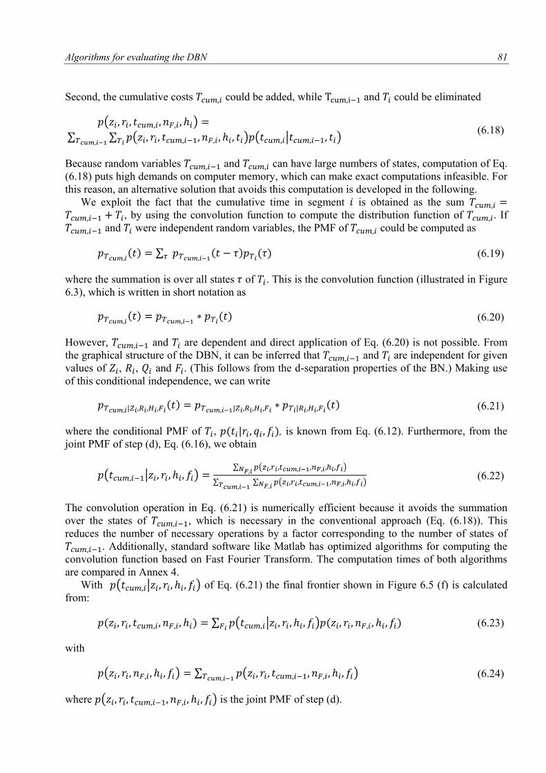
Algorithms for evaluating the DBN 81
Second, the cumulative costs could be added, while and could be eliminated
( )
∑ ∑ ( ) ( | )
(6.18)
Because random variables and can have large numbers of states, computation of Eq.
(6.18) puts high demands on computer memory, which can make exact computations infeasible. For
this reason, an alternative solution that avoids this computation is developed in the following.
We exploit the fact that the cumulative time in segment is obtained as the sum , by using the convolution function to compute the distribution function of . If
and were independent random variables, the PMF of could be computed as
∑
(6.19)
where the summation is over all states of . This is the convolution function (illustrated in Figure
6.3), which is written in short notation as
(6.20)
However, and are dependent and direct application of Eq. (6.20) is not possible. From
the graphical structure of the DBN, it can be inferred that and are independent for given
values of , , and . (This follows from the d-separation properties of the BN.) Making use
of this conditional independence, we can write
| |
| (6.21)
where the conditional PMF of , | , is known from Eq. (6.12). Furthermore, from the
joint PMF of step (d), Eq. (6.16), we obtain
( | ) ∑ ( )
∑ ∑ ( )
(6.22)
The convolution operation in Eq. (6.21) is numerically efficient because it avoids the summation
over the states of , which is necessary in the conventional approach (Eq. (6.18)). This
reduces the number of necessary operations by a factor corresponding to the number of states of
. Additionally, standard software like Matlab has optimized algorithms for computing the
convolution function based on Fast Fourier Transform. The computation times of both algorithms
are compared in Annex 4.
With ( | ) of Eq. (6.21) the final frontier shown in Figure 6.5 (f) is calculated
from:
∑ ( | ) (6.23)
with
( ) ∑ ( ) (6.24)
where ( ) is the joint PMF of step (d).
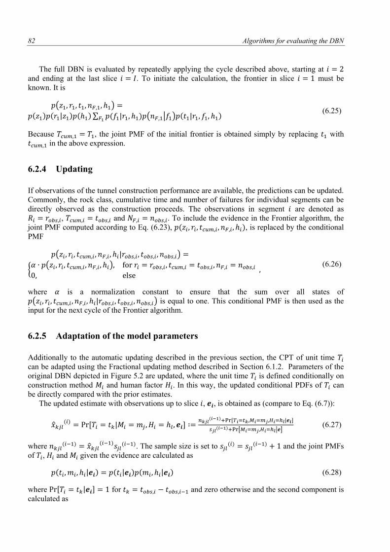
82 Algorithms for evaluating the DBN
The full DBN is evaluated by repeatedly applying the cycle described above, starting at
and ending at the last slice . To initiate the calculation, the frontier in slice must be
known. It is
( )
| ∑ | ( | ) | (6.25)
Because , the joint PMF of the initial frontier is obtained simply by replacing with
in the above expression.
6.2.4 Updating
If observations of the tunnel construction performance are available, the predictions can be updated.
Commonly, the rock class, cumulative time and number of failures for individual segments can be
directly observed as the construction proceeds. The observations in segment are denoted as
, and . To include the evidence in the Frontier algorithm, the
joint PMF computed according to Eq. (6.23), , is replaced by the conditional
PMF
( | )
{ ( )
(6.26)
where is a normalization constant to ensure that the sum over all states of
( | ) is equal to one. This conditional PMF is then used as the
input for the next cycle of the Frontier algorithm.
6.2.5 Adaptation of the model parameters
Additionally to the automatic updating described in the previous section, the CPT of unit time
can be adapted using the Fractional updating method described in Section 6.1.2. Parameters of the
original DBN depicted in Figure 5.2 are updated, where the unit time is defined conditionally on
construction method and human factor . In this way, the updated conditional PDFs of can
be directly compared with the prior estimates.
The updated estimate with observations up to slice , , is obtained as (compare to Eq. (6.7)):
[ | ]
[ | ]
[ | ]
(6.27)
where
. The sample size is set to
and the joint PMFs
of , and given the evidence are calculated as
| | | (6.28)
where [ | ] for and zero otherwise and the second component is
calculated as
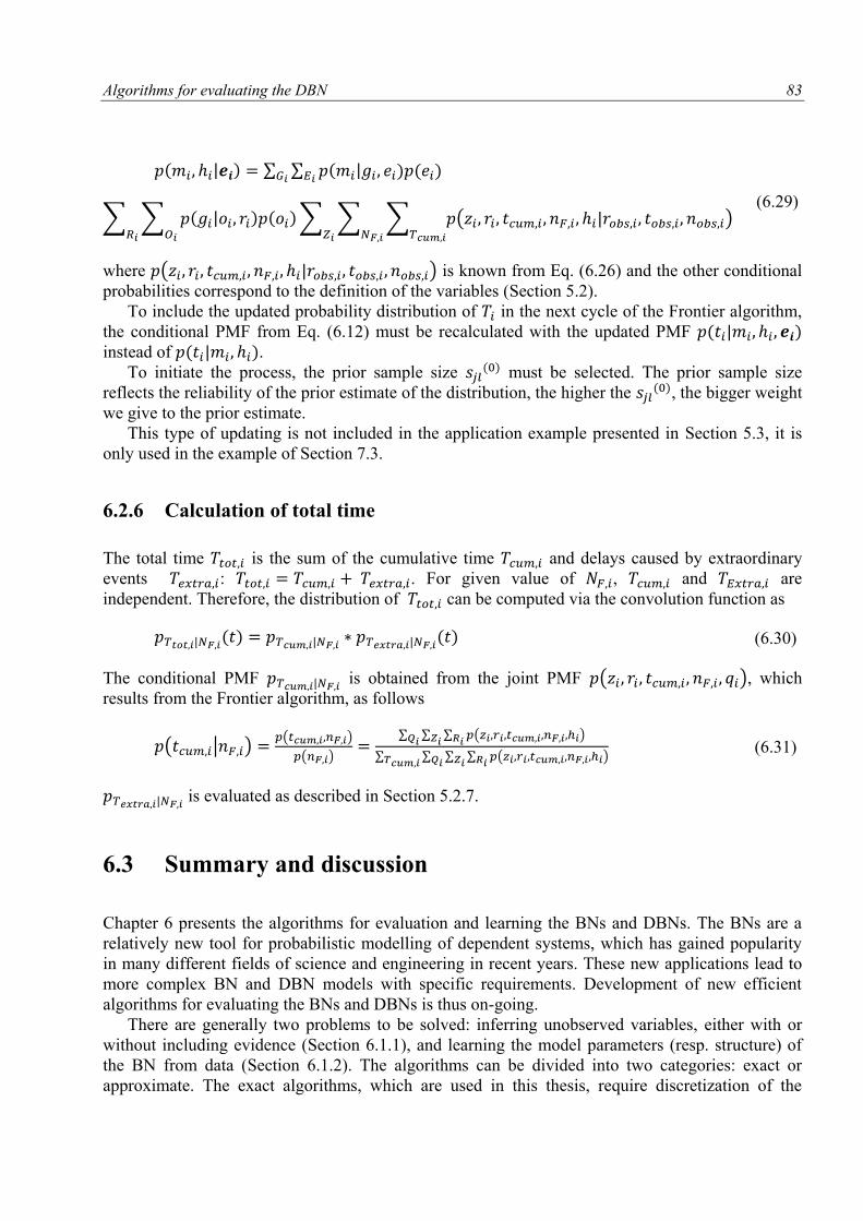
Algorithms for evaluating the DBN 83
| ∑ ∑ |
∑ ∑ | ∑ ∑ ∑ ( | )
(6.29)
where ( | ) is known from Eq. (6.26) and the other conditional
probabilities correspond to the definition of the variables (Section 5.2).
To include the updated probability distribution of in the next cycle of the Frontier algorithm,
the conditional PMF from Eq. (6.12) must be recalculated with the updated PMF |
instead of | . To initiate the process, the prior sample size
must be selected. The prior sample size
reflects the reliability of the prior estimate of the distribution, the higher the , the bigger weight
we give to the prior estimate.
This type of updating is not included in the application example presented in Section 5.3, it is
only used in the example of Section 7.3.
6.2.6 Calculation of total time
The total time is the sum of the cumulative time and delays caused by extraordinary
events : . For given value of , and are
independent. Therefore, the distribution of can be computed via the convolution function as
| |
| (6.30)
The conditional PMF | is obtained from the joint PMF ( ), which
results from the Frontier algorithm, as follows
( | ) ( )
( )
∑ ∑ ∑ ( )
∑ ∑ ∑ ∑ ( )
(6.31)
| is evaluated as described in Section 5.2.7.
6.3 Summary and discussion
Chapter 6 presents the algorithms for evaluation and learning the BNs and DBNs. The BNs are a
relatively new tool for probabilistic modelling of dependent systems, which has gained popularity
in many different fields of science and engineering in recent years. These new applications lead to
more complex BN and DBN models with specific requirements. Development of new efficient
algorithms for evaluating the BNs and DBNs is thus on-going.
There are generally two problems to be solved: inferring unobserved variables, either with or
without including evidence (Section 6.1.1), and learning the model parameters (resp. structure) of
the BN from data (Section 6.1.2). The algorithms can be divided into two categories: exact or
approximate. The exact algorithms, which are used in this thesis, require discretization of the
84 Algorithms for evaluating the DBN
continuous random variables in the network, e.g. following the procedure described in Section
6.1.3.
The specific procedure for evaluating the DBN model proposed in this thesis is described in
Section 6.2. The novel contribution described in this chapter is the modified Frontier algorithm
(Section 6.2.3). Two modifications to the original FA (Section 6.1.4) are proposed, which avoid
defining large conditional probability tables: (a) the frontier is optimized by excluding some of the
variables; this modification was originally proposed by Murphy (2002) under the name “interface
algorithm”; (b) some steps of the original algorithm are replaced by computations of convolutions
of conditional PMFs; to our knowledge, this modification has not been previously published. The
new algorithm is computationally efficient; computations shown here were performed in Matlab
and take in the order of 80 CPU seconds on a MacBook Pro with a 2.53 GHz Intel Core 2 Duo
Processor, 4 GB 1067 MHz DDR3 RAM and Mac OS X v. 10.6.8. The computational efficiency of
the modified Frontier algorithms in comparison with the original Frontier algorithm is presented in
Annex 4.
85
To obtain realistic results from the probabilistic modelling, it is essential to properly describe the
model parameters. As was discussed in Section 3.2, the majority of probabilistic models of
construction processes rely on expert assessment of the inputs. The unit cost and activity durations
or advance rates are commonly described using uniform, triangular or beta distribution (Min, 2003;
van Dorp, 2005; Yang, 2007; Project Management Institute, 2008; Said et al., 2009). Triangular and
uniform distributions are especially popular, because the experts feel generally comfortable in
assessing the boundary values resp. mean/mode of the variables. Studies analysing the data from
construction projects, however, show that other probabilistic models, such as lognormal or Weibull
distribution, are more suitable (Wall, 1997; Chou, 2011).
In this section, data from tunnels constructed in the past are statistically analysed in order to
obtain realistic description of model parameters. Only data on construction time are analysed,
information on construction costs were not available. It is proposed to categorize the performance
of the excavation process in three classes: (1) Normal performance, where the excavation round is
commonly finished within one day. (2) Small disturbances of the process associated with delays in
the order of a few days. (3) Extraordinary events, corresponding to cases when the excavation
stopped for longer than 15 days.
The statistics of normal performance (1) and small disturbances (2) can be assessed from the
observed excavation performance. Such analyses are presented in Section 7.1 using data from three
tunnels in the Czech Republic. The analysis includes selection of an appropriate probabilistic model
and analysis of correlations of the construction process. For extraordinary events (3), statistical
analysis is only meaningful if it is based on a larger dataset including a large number of tunnel
projects, as presented in Section 7.2.
The findings of the data analysis are used in the application example of Section 7.3. The DBN
model presented in Chapter 5 is used to model the construction time of tunnel TUN3. Inputs of the
model are determined with regard to the results of data analysis. TUN3 was used already in case
study of Section 4.2, where the risk of extraordinary events and partly also small disturbances was
7 Analysis of tunnel construction data
for learning the model parameters
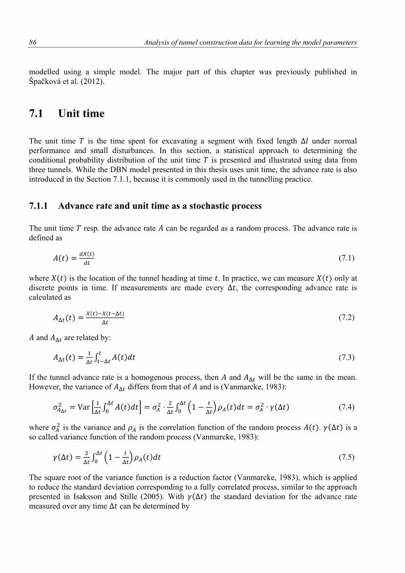
86 Analysis of tunnel construction data for learning the model parameters
modelled using a simple model. The major part of this chapter was previously published in
Špačková et al. (2012).
7.1 Unit time
The unit time is the time spent for excavating a segment with fixed length under normal
performance and small disturbances. In this section, a statistical approach to determining the
conditional probability distribution of the unit time is presented and illustrated using data from
three tunnels. While the DBN model presented in this thesis uses unit time, the advance rate is also
introduced in the Section 7.1.1, because it is commonly used in the tunnelling practice.
7.1.1 Advance rate and unit time as a stochastic process
The unit time resp. the advance rate can be regarded as a random process. The advance rate is
defined as
(7.1)
where is the location of the tunnel heading at time . In practice, we can measure only at
discrete points in time. If measurements are made every , the corresponding advance rate is
calculated as
(7.2)
and are related by:
∫
(7.3)
If the tunnel advance rate is a homogenous process, then and will be the same in the mean.
However, the variance of differs from that of and is (Vanmarcke, 1983):
[
∫
]
∫ (
)
(7.4)
where is the variance and is the correlation function of the random process . is a
so called variance function of the random process (Vanmarcke, 1983):
∫ (
)
(7.5)
The square root of the variance function is a reduction factor (Vanmarcke, 1983), which is applied
to reduce the standard deviation corresponding to a fully correlated process, similar to the approach
presented in Isaksson and Stille (2005). With the standard deviation for the advance rate
measured over any time can be determined by
Analysis of tunnel construction data for learning the model parameters 87
√
( ) (7.6)
where is the standard deviation of the advance rate measured over a reference time .
depends on the correlation function. For the special case of an uncorrelated process, it is
; for a fully correlated process it is .
Eqs. (7.3) and (7.4) give rise to the averaging effect: The variance of becomes smaller as
increases. This must be accounted for when estimating the advance rate from observations.
However, in practice this effect is often neglected when advance rates are estimated by experts,
which can lead to significant under- or overestimation of the uncertainty.
In the DBN model, unit time is utilized instead of the advance rate. It is defined as
(7.7)
where is the time the tunnel heading passes the position and is the length of a tunnel
segment.
For a homogenous process, the mean of unit time increases linearly with :
(7.8)
where is the mean of the unit time for a reference length .
The variance of the is also a function of . In analogy to Eq. (7.6), it can be expressed as a
function of , the standard deviation of the unit time for a reference length :
√
( ) (7.9)
where the variance function is:
∫ (
)
(7.10)
where is the correlation function of the unit time. Examples of correlation functions of unit time
along the tunnel axis are derived in Section 7.1.4.
For more details on the analysis of stochastic processes the reader is referred to Vanmarcke
(1983) and Elishakoff (1999).
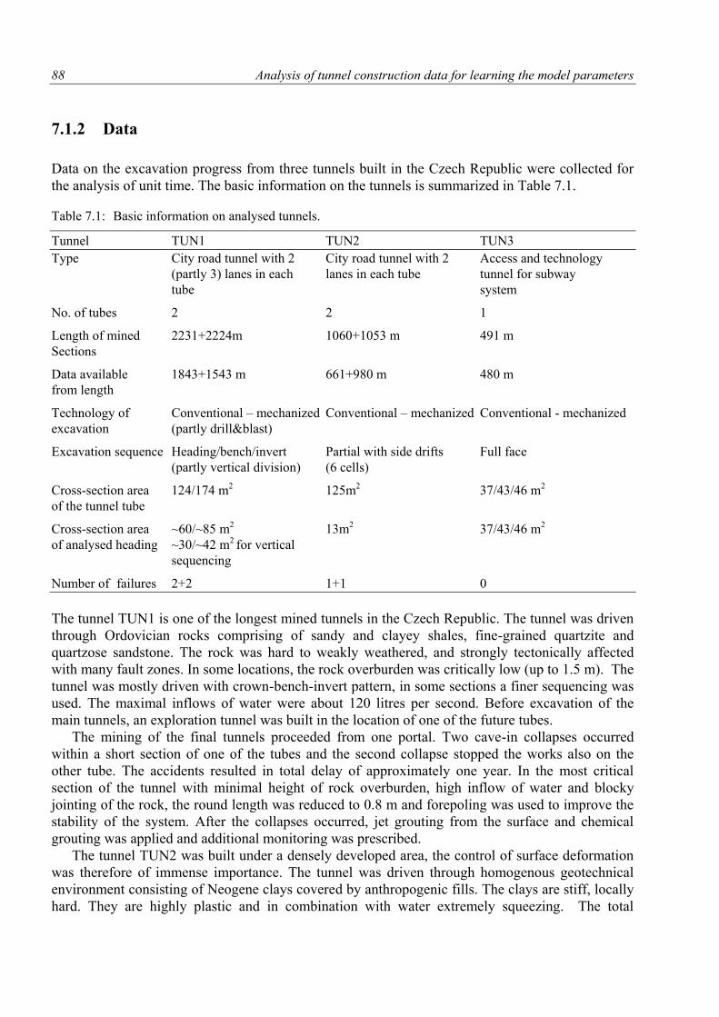
88 Analysis of tunnel construction data for learning the model parameters
7.1.2 Data
Data on the excavation progress from three tunnels built in the Czech Republic were collected for
the analysis of unit time. The basic information on the tunnels is summarized in Table 7.1.
Table 7.1: Basic information on analysed tunnels.
Tunnel TUN1 TUN2 TUN3
Type City road tunnel with 2 City road tunnel with 2 Access and technology
(partly 3) lanes in each lanes in each tube tunnel for subway
tube system
No. of tubes 2 2 1
Length of mined 2231+2224m 1060+1053 m 491 m
Sections
Data available 1843+1543 m 661+980 m 480 m
from length
Technology of Conventional – mechanized Conventional – mechanized Conventional - mechanized
excavation (partly drill&blast)
Excavation sequence Heading/bench/invert Partial with side drifts Full face
(partly vertical division) (6 cells)
Cross-section area 124/174 m2 125m2 37/43/46 m2
of the tunnel tube
Cross-section area ~60/~85 m2 13m2 37/43/46 m2
of analysed heading ~30/~42 m2 for vertical
sequencing
Number of failures 2+2 1+1 0
The tunnel TUN1 is one of the longest mined tunnels in the Czech Republic. The tunnel was driven
through Ordovician rocks comprising of sandy and clayey shales, fine-grained quartzite and
quartzose sandstone. The rock was hard to weakly weathered, and strongly tectonically affected
with many fault zones. In some locations, the rock overburden was critically low (up to 1.5 m). The
tunnel was mostly driven with crown-bench-invert pattern, in some sections a finer sequencing was
used. The maximal inflows of water were about 120 litres per second. Before excavation of the
main tunnels, an exploration tunnel was built in the location of one of the future tubes.
The mining of the final tunnels proceeded from one portal. Two cave-in collapses occurred
within a short section of one of the tubes and the second collapse stopped the works also on the
other tube. The accidents resulted in total delay of approximately one year. In the most critical
section of the tunnel with minimal height of rock overburden, high inflow of water and blocky
jointing of the rock, the round length was reduced to 0.8 m and forepoling was used to improve the
stability of the system. After the collapses occurred, jet grouting from the surface and chemical
grouting was applied and additional monitoring was prescribed.
The tunnel TUN2 was built under a densely developed area, the control of surface deformation
was therefore of immense importance. The tunnel was driven through homogenous geotechnical
environment consisting of Neogene clays covered by anthropogenic fills. The clays are stiff, locally
hard. They are highly plastic and in combination with water extremely squeezing. The total
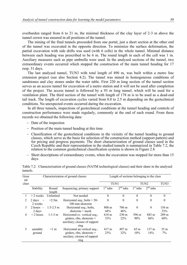
Analysis of tunnel construction data for learning the model parameters 89
overburden ranged from 6 to 21 m, the minimal thickness of the clay layer of 2-3 m above the
tunnel crown was ensured in all positions of the tunnel.
The mining of the final tunnels proceeded from one portal, just a short section at the other end
of the tunnel was excavated in the opposite direction. To minimize the surface deformation, the
partial excavation with side drifts was used (with 6 cells) in the whole tunnel. Minimal distance
between each heading was prescribed to be 6 m. The round length in each of the cell was 1 m.
Auxiliary measures such as pipe umbrella were used. In the analysed sections of the tunnel, two
extraordinary events occurred which stopped the construction of the main tunnel heading for 17
resp. 31 days.
The last analysed tunnel, TUN3 with total length of 490 m, was built within a metro line
extension project (see also Section 4.2). The tunnel was mined in homogeneous conditions of
sandstones and clay stones under the water table. First 220 m long section of the tunnel section
serves as an access tunnel for excavation of a metro station and it will not be used after completion
of the project. The access tunnel is followed by a 93 m long tunnel, which will be used for a
ventilation plant. The third section of the tunnel with length of 178 m is to be used as a dead-end
tail track. The length of excavation cycles varied from 0.8 to 2.5 m depending on the geotechnical
conditions. No unexpected events occurred during the excavation.
In all three tunnels, inspections of geotechnical conditions at the tunnel heading and controls of
construction performance were made regularly, commonly at the end of each round. From these
records we obtained the following data:
Date of the inspection
Position of the main tunnel heading at this time
Classification of the geotechnical conditions in the vicinity of the tunnel heading to ground classes, which serve as the basis for selection of the construction method (support pattern) and for pricing and progress payments. The short characterization of ground classes used in the Czech Republic and their representation in the studied tunnels is summarized in Table 7.2, the relation to the common geotechnical classification systems is shown in Figure 2.8
Short descriptions of extraordinary events, when the excavation was stopped for more than 15 days.
Table 7.2: Characterization of ground classes (NATM technological classes) and their share in the analysed
tunnels.
Grou
nd
class
Characterization of ground classes Length of sections belonging to the class
TUN1 TUN2 TUN3
Stability Round
length
Sequencing; primary support 1st tube 2nd tube 1st tube 2nd tube
1 > 2 weeks Unlimited Not needed 0 0 0 0 0
2 2 days -
2 weeks
>2.5m Horizontal seq.; bolts + 50-
100 mm shotcrete
0 0 0 0 0
3 2 hours -
2 days
1.5-2.5 m Horizontal seq.; bolts,
shotcrete + mesh
808 m
44%
706 m
46%
0 0 156 m
33%
4 < 2 hours 1-1.5 m Horizontal ev. vertical seq.;
girders, ribs, shotcrete +
auxiliary; closure of support
ring
618 m
33%
230 m
22%
596 m
90%
843 m
86%
289 m
60%
5 unstable
ground
<1 m Horizontal an vertical seq.;
girders, ribs, shotcrete +
auxilary; closure of support
ring
417 m
23%
497 m
32%
65 m
10%
137 m
14%
35 m
7%
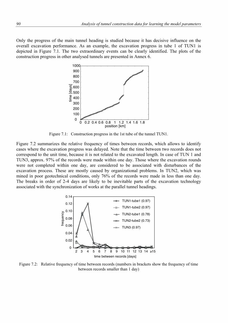
90 Analysis of tunnel construction data for learning the model parameters
Only the progress of the main tunnel heading is studied because it has decisive influence on the
overall excavation performance. As an example, the excavation progress in tube 1 of TUN1 is
depicted in Figure 7.1. The two extraordinary events can be clearly identified. The plots of the
construction progress in other analysed tunnels are presented in Annex 6.
Figure 7.1: Construction progress in the 1st tube of the tunnel TUN1.
Figure 7.2 summarizes the relative frequency of times between records, which allows to identify
cases where the excavation progress was delayed. Note that the time between two records does not
correspond to the unit time, because it is not related to the excavated length. In case of TUN 1 and
TUN3, approx. 97% of the records were made within one day. Those where the excavation rounds
were not completed within one day, are considered to be associated with disturbances of the
excavation process. These are mostly caused by organizational problems. In TUN2, which was
mined in poor geotechnical conditions, only 76% of the records were made in less than one day.
The breaks in order of 2-4 days are likely to be inevitable parts of the excavation technology
associated with the synchronization of works at the parallel tunnel headings.
Figure 7.2: Relative frequency of time between records (numbers in brackets show the frequency of time
between records smaller than 1 day)
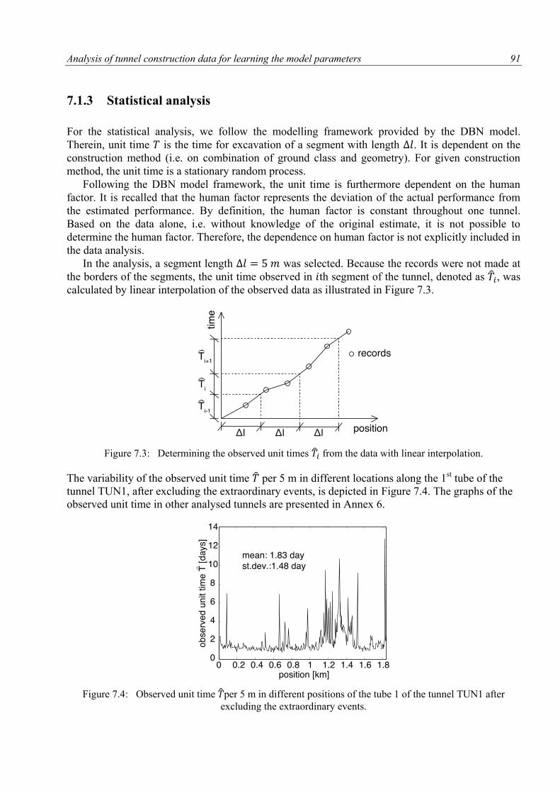
Analysis of tunnel construction data for learning the model parameters 91
7.1.3 Statistical analysis
For the statistical analysis, we follow the modelling framework provided by the DBN model.
Therein, unit time is the time for excavation of a segment with length . It is dependent on the
construction method (i.e. on combination of ground class and geometry). For given construction
method, the unit time is a stationary random process.
Following the DBN model framework, the unit time is furthermore dependent on the human
factor. It is recalled that the human factor represents the deviation of the actual performance from
the estimated performance. By definition, the human factor is constant throughout one tunnel.
Based on the data alone, i.e. without knowledge of the original estimate, it is not possible to
determine the human factor. Therefore, the dependence on human factor is not explicitly included in
the data analysis.
In the analysis, a segment length was selected. Because the records were not made at
the borders of the segments, the unit time observed in th segment of the tunnel, denoted as , was
calculated by linear interpolation of the observed data as illustrated in Figure 7.3.
Figure 7.3: Determining the observed unit times from the data with linear interpolation.
The variability of the observed unit time per 5 m in different locations along the 1st tube of the
tunnel TUN1, after excluding the extraordinary events, is depicted in Figure 7.4. The graphs of the
observed unit time in other analysed tunnels are presented in Annex 6.
Figure 7.4: Observed unit time per 5 m in different positions of the tube 1 of the tunnel TUN1 after
excluding the extraordinary events.
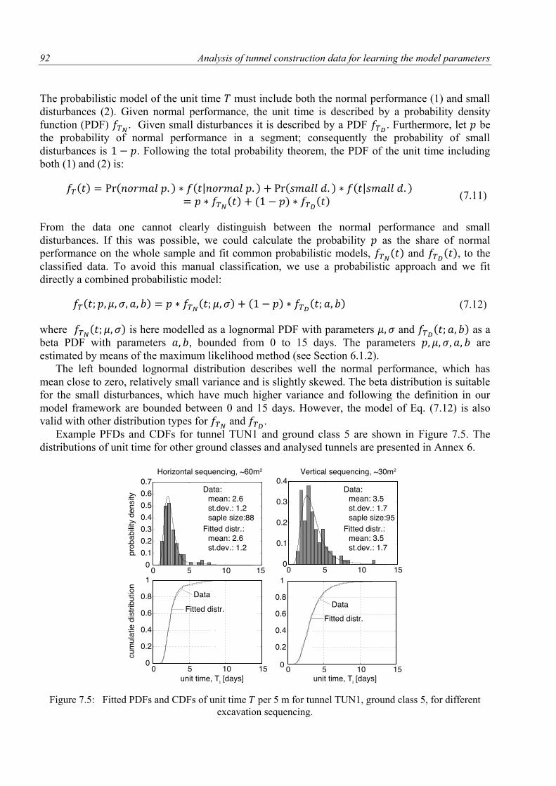
92 Analysis of tunnel construction data for learning the model parameters
The probabilistic model of the unit time must include both the normal performance (1) and small
disturbances (2). Given normal performance, the unit time is described by a probability density
function (PDF) . Given small disturbances it is described by a PDF
. Furthermore, let be
the probability of normal performance in a segment; consequently the probability of small
disturbances is . Following the total probability theorem, the PDF of the unit time including
both (1) and (2) is:
| |
(7.11)
From the data one cannot clearly distinguish between the normal performance and small
disturbances. If this was possible, we could calculate the probability as the share of normal
performance on the whole sample and fit common probabilistic models, and
, to the
classified data. To avoid this manual classification, we use a probabilistic approach and we fit
directly a combined probabilistic model:
(7.12)
where is here modelled as a lognormal PDF with parameters and
as a
beta PDF with parameters , bounded from 0 to 15 days. The parameters are
estimated by means of the maximum likelihood method (see Section 6.1.2).
The left bounded lognormal distribution describes well the normal performance, which has
mean close to zero, relatively small variance and is slightly skewed. The beta distribution is suitable
for the small disturbances, which have much higher variance and following the definition in our
model framework are bounded between 0 and 15 days. However, the model of Eq. (7.12) is also
valid with other distribution types for and
.
Example PFDs and CDFs for tunnel TUN1 and ground class 5 are shown in Figure 7.5. The
distributions of unit time for other ground classes and analysed tunnels are presented in Annex 6.
Figure 7.5: Fitted PDFs and CDFs of unit time per 5 m for tunnel TUN1, ground class 5, for different
excavation sequencing.
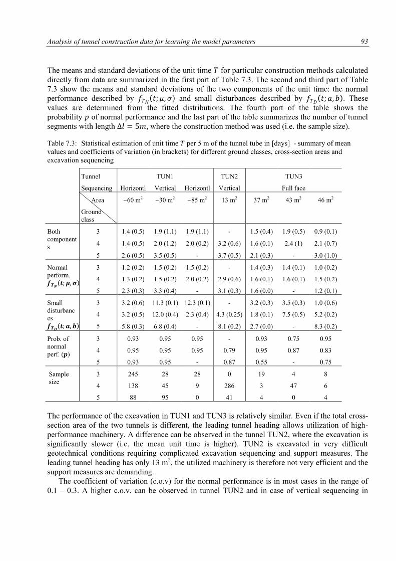
Analysis of tunnel construction data for learning the model parameters 93
The means and standard deviations of the unit time for particular construction methods calculated
directly from data are summarized in the first part of Table 7.3. The second and third part of Table
7.3 show the means and standard deviations of the two components of the unit time: the normal
performance described by and small disturbances described by
. These
values are determined from the fitted distributions. The fourth part of the table shows the
probability of normal performance and the last part of the table summarizes the number of tunnel
segments with length , where the construction method was used (i.e. the sample size).
Table 7.3: Statistical estimation of unit time per 5 m of the tunnel tube in [days] - summary of mean
values and coefficients of variation (in brackets) for different ground classes, cross-section areas and
excavation sequencing
Tunnel TUN1 TUN2 TUN3
Sequencing Horizontl Vertical Horizontl Vertical Full face
Area
Ground
class
~60 m2 ~30 m2 ~85 m2 13 m2 37 m2 43 m2 46 m2
Both
component
s
3 1.4 (0.5) 1.9 (1.1) 1.9 (1.1) - 1.5 (0.4) 1.9 (0.5) 0.9 (0.1)
4 1.4 (0.5) 2.0 (1.2) 2.0 (0.2) 3.2 (0.6) 1.6 (0.1) 2.4 (1) 2.1 (0.7)
5 2.6 (0.5) 3.5 (0.5) - 3.7 (0.5) 2.1 (0.3) - 3.0 (1.0)
Normal
perform.
3 1.2 (0.2) 1.5 (0.2) 1.5 (0.2) - 1.4 (0.3) 1.4 (0.1) 1.0 (0.2)
4 1.3 (0.2) 1.5 (0.2) 2.0 (0.2) 2.9 (0.6) 1.6 (0.1) 1.6 (0.1) 1.5 (0.2)
5 2.3 (0.3) 3.3 (0.4) - 3.1 (0.3) 1.6 (0.0) - 1.2 (0.1)
Small
disturbanc
es
3 3.2 (0.6) 11.3 (0.1) 12.3 (0.1) - 3.2 (0.3) 3.5 (0.3) 1.0 (0.6)
4 3.2 (0.5) 12.0 (0.4) 2.3 (0.4) 4.3 (0.25) 1.8 (0.1) 7.5 (0.5) 5.2 (0.2)
5 5.8 (0.3) 6.8 (0.4) - 8.1 (0.2) 2.7 (0.0) - 8.3 (0.2)
Prob. of
normal
perf. ( )
3 0.93 0.95 0.95 - 0.93 0.75 0.95
4 0.95 0.95 0.95 0.79 0.95 0.87 0.83
5 0.93 0.95 - 0.87 0.55 - 0.75
Sample
size
3 245 28 28 0 19 4 8
4 138 45 9 286 3 47 6
5 88 95 0 41 4 0 4
The performance of the excavation in TUN1 and TUN3 is relatively similar. Even if the total cross-
section area of the two tunnels is different, the leading tunnel heading allows utilization of high-
performance machinery. A difference can be observed in the tunnel TUN2, where the excavation is
significantly slower (i.e. the mean unit time is higher). TUN2 is excavated in very difficult
geotechnical conditions requiring complicated excavation sequencing and support measures. The
leading tunnel heading has only 13 m2, the utilized machinery is therefore not very efficient and the
support measures are demanding.
The coefficient of variation (c.o.v) for the normal performance is in most cases in the range of
0.1 – 0.3. A higher c.o.v. can be observed in tunnel TUN2 and in case of vertical sequencing in
94 Analysis of tunnel construction data for learning the model parameters
tunnel TUN1. This indicates that for demanding excavation technologies the variability of the
performance is increased.
Excluding the cases for which the sample size is insufficient, we can conclude that the
probability of normal performance, as expressed by the parameter , is in the order of 0.8 to 0.95. It
is noted that the estimated values of correspond well to the observed frequencies of time between
records shown in Figure 7.2.
For several construction methods, the data basis is not sufficient for reliably estimating the
parameters of . Nevertheless, the analysis shows that the small disturbances can explain the
difference between the c.o.v. of the observed unit time and the c.o.v. of the normal performance.
The latter is the value that most experts would estimate.
7.1.4 Correlation analysis
In addition to assessing the marginal distribution of unit time, it is necessary to analyse the
correlation of construction performance among different locations. For this analysis, the unit time
per 1 m of tunnel tube, denoted as , is evaluated. The sample coefficient of correlation of the
unit time for two segments at a distance is calculated as:
∑
(7.13)
where and are the sample mean and standard deviation of , is the unit time
observed at position and is the unit time observed at position . is the number of
observations: , where is the length of the tunnel tube excavated with a given
construction method.
A power-exponential function is fitted to the observed correlation coefficient:
(7.14)
where and are the parameters to be fitted. is a correlation function (Vanmarcke, 1983).
Other correlation functions were investigated, but the power-exponential function was found to best
describe the data from the analysed tunnels.
Figure 7.6 depicts the observed correlation function for unit time , calculated from data of
geotechnical class 4.
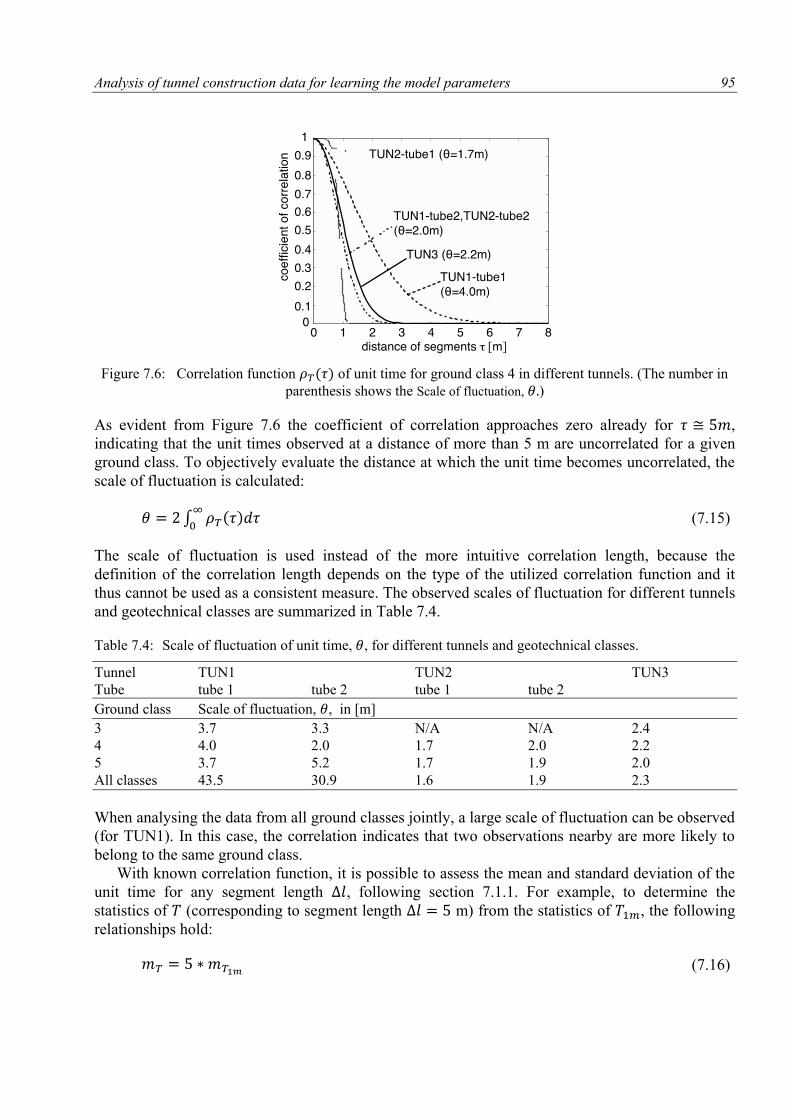
Analysis of tunnel construction data for learning the model parameters 95
Figure 7.6: Correlation function of unit time for ground class 4 in different tunnels. (The number in
parenthesis shows the Scale of fluctuation, )
As evident from Figure 7.6 the coefficient of correlation approaches zero already for ,
indicating that the unit times observed at a distance of more than 5 m are uncorrelated for a given
ground class. To objectively evaluate the distance at which the unit time becomes uncorrelated, the
scale of fluctuation is calculated:
∫
(7.15)
The scale of fluctuation is used instead of the more intuitive correlation length, because the
definition of the correlation length depends on the type of the utilized correlation function and it
thus cannot be used as a consistent measure. The observed scales of fluctuation for different tunnels
and geotechnical classes are summarized in Table 7.4.
Table 7.4: Scale of fluctuation of unit time, , for different tunnels and geotechnical classes.
Tunnel TUN1 TUN2 TUN3
Tube tube 1 tube 2 tube 1 tube 2
Ground class Scale of fluctuation, , in [m]
3 3.7 3.3 N/A N/A 2.4
4 4.0 2.0 1.7 2.0 2.2
5 3.7 5.2 1.7 1.9 2.0
All classes 43.5 30.9 1.6 1.9 2.3
When analysing the data from all ground classes jointly, a large scale of fluctuation can be observed
(for TUN1). In this case, the correlation indicates that two observations nearby are more likely to
belong to the same ground class.
With known correlation function, it is possible to assess the mean and standard deviation of the
unit time for any segment length , following section 7.1.1. For example, to determine the
statistics of (corresponding to segment length m) from the statistics of , the following
relationships hold:
(7.16)
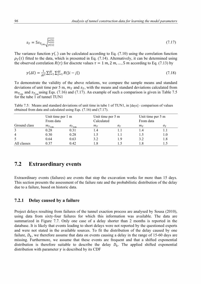
96 Analysis of tunnel construction data for learning the model parameters
√
(7.17)
The variance function can be calculated according to Eq. (7.10) using the correlation function
fitted to the data, which is presented in Eq. (7.14). Alternatively, it can be determined using
the observed correlation for discrete values according to Eq. (7.13) by
∑ ∑ | |
(7.18)
To demonstrate the validity of the above relations, we compare the sample means and standard
deviations of unit time per 5 m, and , with the means and standard deviations calculated from
and using Eqs. (7.16) and (7.17). An example of such a comparison is given in Table 7.5
for the tube 1 of tunnel TUN1
Table 7.5: Means and standard deviations of unit time in tube 1 of TUN1, in [days] - comparison of values
obtained from data and calculated using Eqs. (7.16) and (7.17).
Unit time per 1 m Unit time per 5 m Unit time per 5 m
From data Calculated From data
Ground class
3 0.28 0.31 1.4 1.1 1.4 1.1
4 0.30 0.28 1.5 1.1 1.5 1.0
5 0.64 0.63 3.2 1.9 3.2 1.8
All classes 0.37 0.42 1.8 1.5 1.8 1.5
7.2 Extraordinary events
Extraordinary events (failures) are events that stop the excavation works for more than 15 days.
This section presents the assessment of the failure rate and the probabilistic distribution of the delay
due to a failure, based on historic data.
7.2.1 Delay caused by a failure
Project delays resulting from failures of the tunnel exaction process are analysed by Sousa (2010),
using data from sixty-four failures for which this information was available. The data are
summarized in Figure 7.7. Only one case of a delay shorter than 2 months is reported in the
database. It is likely that events leading to short delays were not reported by the questioned experts
and were not stated in the available sources. To fit the distribution of the delay caused by one
failure, , we therefore assume that data on events causing a delay in the range of 15-60 days are
missing. Furthermore, we assume that these events are frequent and that a shifted exponential
distribution is therefore suitable to describe the delay . The applied shifted exponential
distribution with parameter is described by its CDF
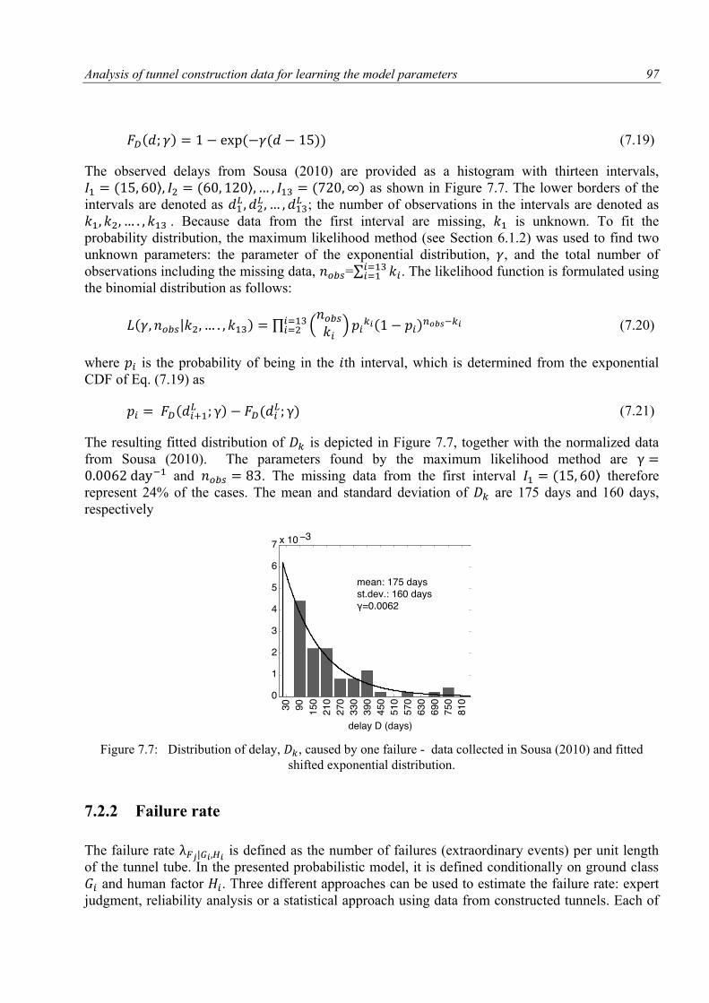
Analysis of tunnel construction data for learning the model parameters 97
(7.19)
The observed delays from Sousa (2010) are provided as a histogram with thirteen intervals,
⟩ ⟩ as shown in Figure 7.7. The lower borders of the
intervals are denoted as
; the number of observations in the intervals are denoted as
. Because data from the first interval are missing, is unknown. To fit the
probability distribution, the maximum likelihood method (see Section 6.1.2) was used to find two
unknown parameters: the parameter of the exponential distribution, , and the total number of
observations including the missing data, =∑ . The likelihood function is formulated using
the binomial distribution as follows:
| ∏ (
)
(7.20)
where is the probability of being in the th interval, which is determined from the exponential
CDF of Eq. (7.19) as
(7.21)
The resulting fitted distribution of is depicted in Figure 7.7, together with the normalized data
from Sousa (2010). The parameters found by the maximum likelihood method are and . The missing data from the first interval ⟩ therefore
represent 24% of the cases. The mean and standard deviation of are 175 days and 160 days,
respectively
Figure 7.7: Distribution of delay, , caused by one failure - data collected in Sousa (2010) and fitted
shifted exponential distribution.
7.2.2 Failure rate
The failure rate | is defined as the number of failures (extraordinary events) per unit length
of the tunnel tube. In the presented probabilistic model, it is defined conditionally on ground class
and human factor . Three different approaches can be used to estimate the failure rate: expert
judgment, reliability analysis or a statistical approach using data from constructed tunnels. Each of
98 Analysis of tunnel construction data for learning the model parameters
the approaches has its strengths and weaknesses. Ideally, several approaches should be used and the
results should be compared and critically examined.
Expert estimations of probabilities of rare events are commonly not reliable. They can be
strongly biased by recent experiences (either positive or negative) of the expert and by many other
factors (Lin and Bier, 2008; Goodwin and Wright, 2010). Such estimates should therefore be
supported by other types of analyses and/or statistical data.
Reliability analysis of tunnel excavation processes is a highly complex task and it is possible
only with strong simplifications. Compared to the analysis of a completed structure, the analysis of
a tunnel excavation process must take into account additional uncertainties connected with the
construction process. One needs not only to analyse the reliability of the final tunnel, but the
reliability of each of the interim states of the process (different levels of support, different phases of
excavation). Additionally, uncertainties resulting from the influence of human and organizational
factors, which are of crucial importance during the construction process, are not included in
common reliability analysis (Blockley, 1999).
In the following, a rough estimate of failure rates using data available in the literature is
presented. The most comprehensive database known to the authors is presented in Sousa (2010);
other databases considered are HSE ( 2006), Seidenfuss (2006) and Stallmann (2005) – see also
Section 2.5.
To determine | based on data, one must know the total number of failure events and the
total length of excavated tunnels, ideally separately for individual ground classes. Because failures
are rare events, data collected from a large number of tunnels would be needed. A rough estimate of
| based on global data is made and compared with estimates using data from the Czech
Republic. Because no information is available on the geological conditions and other features of the
included tunnels, only the unconditional failure rate can be assessed.
According to HSE (2006), tunnels with a total length of 8750 km were constructed in the years
1999-2004 worldwide, as summarized in Table 7.6, their geographical distribution is displayed in
Figure 7.8. These data were collected from freely accessible websites; their accuracy is limited and
their completeness cannot be verified. For this reason, the data reported for the Czech Republic by
HSE (2006) is compared with detailed information from Barták (2007) and from the overview
presented in Annex 5. HSE (2006) reports construction of 29 tunnels with a total length of 59.6 km
in the Czech Republic in the years 1999-2004. This number overestimates the length of constructed
tunnels by 15% if parallel tunnel tubes are considered as separate tunnels and by 35% if parallel
tubes are considered as one tunnel. Additionally, approximately 15% of the tunnels in the Czech
republic constructed in this period are excavated by the cut&cover method. Assuming that these
shares apply also to the data in other countries, we reduce the total length of tunnels reported in
HSE (2006) to estimate the total length of mined tunnels. The resulting estimates are shown in
Table 7.6.
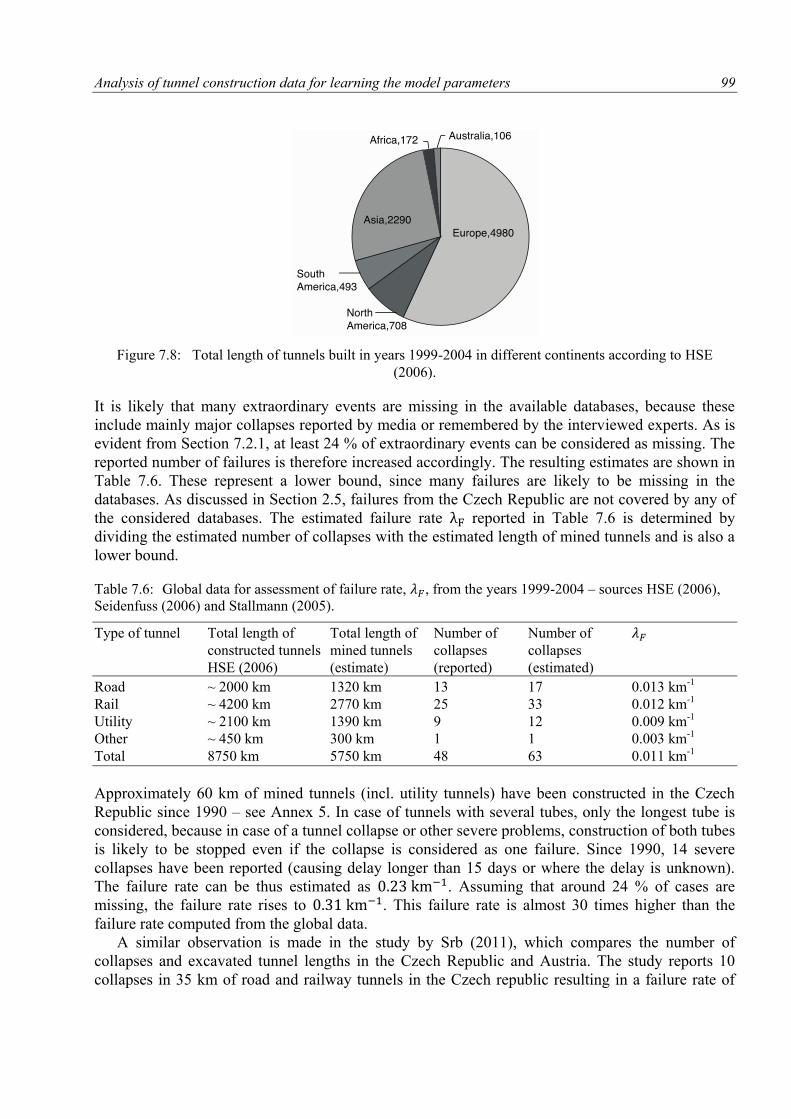
Analysis of tunnel construction data for learning the model parameters 99
Figure 7.8: Total length of tunnels built in years 1999-2004 in different continents according to HSE
(2006).
It is likely that many extraordinary events are missing in the available databases, because these
include mainly major collapses reported by media or remembered by the interviewed experts. As is
evident from Section 7.2.1, at least 24 % of extraordinary events can be considered as missing. The
reported number of failures is therefore increased accordingly. The resulting estimates are shown in
Table 7.6. These represent a lower bound, since many failures are likely to be missing in the
databases. As discussed in Section 2.5, failures from the Czech Republic are not covered by any of
the considered databases. The estimated failure rate reported in Table 7.6 is determined by
dividing the estimated number of collapses with the estimated length of mined tunnels and is also a
lower bound.
Table 7.6: Global data for assessment of failure rate, , from the years 1999-2004 – sources HSE (2006),
Seidenfuss (2006) and Stallmann (2005).
Type of tunnel Total length of Total length of Number of Number of
constructed tunnels mined tunnels collapses collapses
HSE (2006) (estimate) (reported) (estimated)
Road ~ 2000 km 1320 km 13 17 0.013 km-1
Rail ~ 4200 km 2770 km 25 33 0.012 km-1
Utility ~ 2100 km 1390 km 9 12 0.009 km-1
Other ~ 450 km 300 km 1 1 0.003 km-1
Total 8750 km 5750 km 48 63 0.011 km-1
Approximately 60 km of mined tunnels (incl. utility tunnels) have been constructed in the Czech
Republic since 1990 – see Annex 5. In case of tunnels with several tubes, only the longest tube is
considered, because in case of a tunnel collapse or other severe problems, construction of both tubes
is likely to be stopped even if the collapse is considered as one failure. Since 1990, 14 severe
collapses have been reported (causing delay longer than 15 days or where the delay is unknown).
The failure rate can be thus estimated as . Assuming that around 24 % of cases are
missing, the failure rate rises to . This failure rate is almost 30 times higher than the
failure rate computed from the global data.
A similar observation is made in the study by Srb (2011), which compares the number of
collapses and excavated tunnel lengths in the Czech Republic and Austria. The study reports 10
collapses in 35 km of road and railway tunnels in the Czech republic resulting in a failure rate of
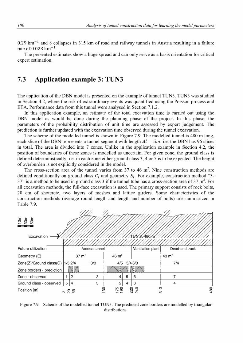
100 Analysis of tunnel construction data for learning the model parameters
and 8 collapses in 315 km of road and railway tunnels in Austria resulting in a failure
rate of .
The presented estimates show a huge spread and can only serve as a basis orientation for critical
expert estimation.
7.3 Application example 3: TUN3
The application of the DBN model is presented on the example of tunnel TUN3. TUN3 was studied
in Section 4.2, where the risk of extraordinary events was quantified using the Poisson process and
ETA. Performance data from this tunnel were analysed in Section 7.1.2.
In this application example, an estimate of the total excavation time is carried out using the
DBN model as would be done during the planning phase of the project. In this phase, the
parameters of the probability distribution of unit time are assessed by expert judgement. The
prediction is further updated with the excavation time observed during the tunnel excavation.
The scheme of the modelled tunnel is shown in Figure 7.9. The modelled tunnel is 480 m long,
each slice of the DBN represents a tunnel segment with length . i.e. the DBN has 96 slices
in total. The area is divided into 7 zones. Unlike in the application example in Section 4.2, the
position of boundaries of these zones is modelled as uncertain. For given zone, the ground class is
defined deterministically, i.e. in each zone either ground class 3, 4 or 5 is to be expected. The height
of overburden is not explicitly considered in the model.
The cross-section area of the tunnel varies from 37 to 46 m2. Nine construction methods are
defined conditionally on ground class and geometry . For example, construction method “3-
37” is a method to be used in ground class 3 if the tunnel tube has a cross-section area of 37 m2. For
all excavation methods, the full-face excavation is used. The primary support consists of rock bolts,
20 cm of shotcrete, two layers of meshes and lattice girders. Some characteristics of the
construction methods (average round length and length and number of bolts) are summarized in
Table 7.9.
Figure 7.9: Scheme of the modelled tunnel TUN3. The predicted zone borders are modelled by triangular
distributions.
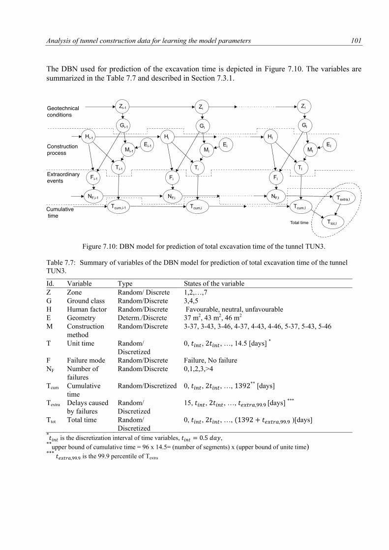
Analysis of tunnel construction data for learning the model parameters 101
The DBN used for prediction of the excavation time is depicted in Figure 7.10. The variables are
summarized in the Table 7.7 and described in Section 7.3.1.
Figure 7.10: DBN model for prediction of total excavation time of the tunnel TUN3.
Table 7.7: Summary of variables of the DBN model for prediction of total excavation time of the tunnel
TUN3.
Id. Variable Type States of the variable
Z Zone Random/ Discrete 1,2,…,7
G Ground class Random/Discrete 3,4,5
H Human factor Random/Discrete Favourable, neutral, unfavourable
E Geometry Determ./Discrete 37 m2, 43 m2, 46 m2
M Construction
method
Random/Discrete 3-37, 3-43, 3-46, 4-37, 4-43, 4-46, 5-37, 5-43, 5-46
T Unit time Random/
Discretized
0, , , …, 14.5 [days] *
F Failure mode Random/Discrete Failure, No failure
NF Number of
failures
Random/Discrete 0,1,2,3,>4
Tcum Cumulative
time
Random/Discretized 0, , , …, ** [days]
Textra Delays caused
by failures
Random/
Discretized
15, , , …, [days] ***
Ttot Total time Random/
Discretized
0, , , …, )[days]
* is the discretization interval of time variables, ,
**upper bound of cumulative time = 96 x 14.5= (number of segments) x (upper bound of unite time)
*** is the 99.9 percentile of Textra
102 Analysis of tunnel construction data for learning the model parameters
7.3.1 Definition of the random variables and numerical inputs
Probabilistic definition of the individual variables follows the one presented in Section 5.2. The
only exception is that in this second application example we do not model the rock class and
overburden (compare the DBNs from Figure 5.2 and Figure 7.10). The ground class is defined
deterministically for the zone by the conditional PMF | 6 as shown in Figure 7.8. For
example, in zone 1 at the beginning of the tunnel, ground class 5 is expected, followed by zone 2
with ground class 4, therefore:
[ | ] and [ | ]
[ | ] and [ | ]
etc.
The positions of zone boundaries are represented by triangular distributions, the parameters of the
distributions are depicted in Figure 7.9 and they are summarized in Table 4.1.
Table 7.8: Parameters of triangular distribution, , describing the location of the end boundaries of the
zones in [m] from the beginning of the tunnel.
Zone Min Mode Max
1 15 20 30
2 35 45 50
3 140 160 180
4 185 200 210
5 215 220 225
6 230 245 260
7 480 480 480
The geometry, , represents the varying cross-section area of the tunnel tube. It is 37 m2 in the first
130 m long section of the tunnel (i.e. in slices of the DBN), 46 m2 in the next 90 m
long section of the tunnel (i.e. in slices of the DBN) and 43 m2 in the last 460 m
long section of the tunnel (i.e. in slices of the DBN).
The construction method is defined deterministically for given and by the conditional
PMF | as shown in Figure 7.8. For example:
[ | ] and [ | ]
[ | ] and [ | ]
The human factor can be in one of three states: “unfavourable, “neutral” and “favourable”. It is
assumed that each of the states has the same probability.
The unit time, , is defined conditionally on construction method and human factor . The
conditional PDFs of unit time are described by combined distributions accordingly with Eq. (7.12).
The parameters of the distributions are assessed by the authors, the parameters of unit time for
are summarized in Table 7.9. The means and standard deviations for both the
6 For direct application of the algorithms described in Section 6.2 it is possible to keep the DBN structure from the
application example 1 (Figure 5.2) and to define the variables as follows: The variable overburden has only one
state; rock class has the same states as ground class and it is defined deterministically for each zone, e.g. [ | ] and [ | ] ; the ground class is defined deterministically conditionally on and , for
example [ | ] and [ | ] .
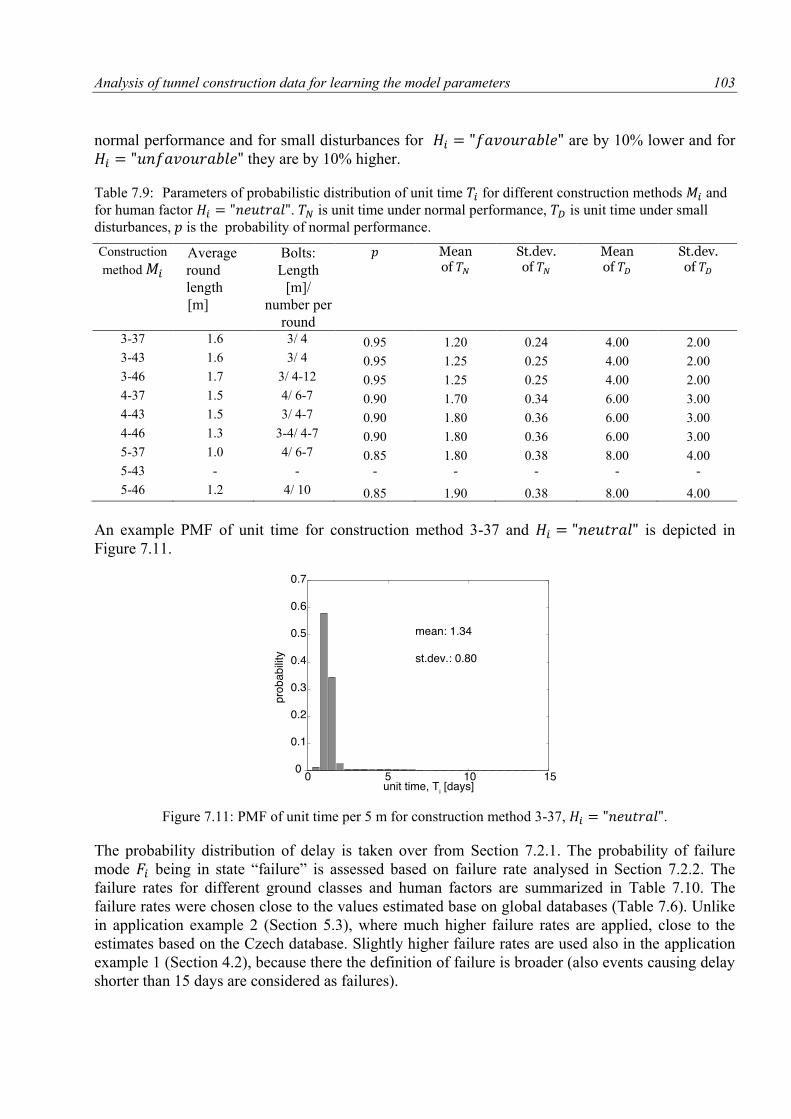
Analysis of tunnel construction data for learning the model parameters 103
normal performance and for small disturbances for are by 10% lower and for
they are by 10% higher.
Table 7.9: Parameters of probabilistic distribution of unit time for different construction methods and
for human factor . is unit time under normal performance, is unit time under small
disturbances, is the probability of normal performance.
Construction
method
Average
round
length
[m]
Bolts:
Length
[m]/
number per
round
Mean of
St.dev. of
Mean of
St.dev. of
3-37 1.6 3/ 4 0.95 1.20 0.24 4.00 2.00
3-43 1.6 3/ 4 0.95 1.25 0.25 4.00 2.00
3-46 1.7 3/ 4-12 0.95 1.25 0.25 4.00 2.00
4-37 1.5 4/ 6-7 0.90 1.70 0.34 6.00 3.00
4-43 1.5 3/ 4-7 0.90 1.80 0.36 6.00 3.00
4-46 1.3 3-4/ 4-7 0.90 1.80 0.36 6.00 3.00
5-37 1.0 4/ 6-7 0.85 1.80 0.38 8.00 4.00
5-43 - - - - - - -
5-46 1.2 4/ 10 0.85 1.90 0.38 8.00 4.00
An example PMF of unit time for construction method 3-37 and is depicted in
Figure 7.11.
Figure 7.11: PMF of unit time per 5 m for construction method 3-37, .
The probability distribution of delay is taken over from Section 7.2.1. The probability of failure
mode being in state “failure” is assessed based on failure rate analysed in Section 7.2.2. The
failure rates for different ground classes and human factors are summarized in Table 7.10. The
failure rates were chosen close to the values estimated base on global databases (Table 7.6). Unlike
in application example 2 (Section 5.3), where much higher failure rates are applied, close to the
estimates based on the Czech database. Slightly higher failure rates are used also in the application
example 1 (Section 4.2), because there the definition of failure is broader (also events causing delay
shorter than 15 days are considered as failures).
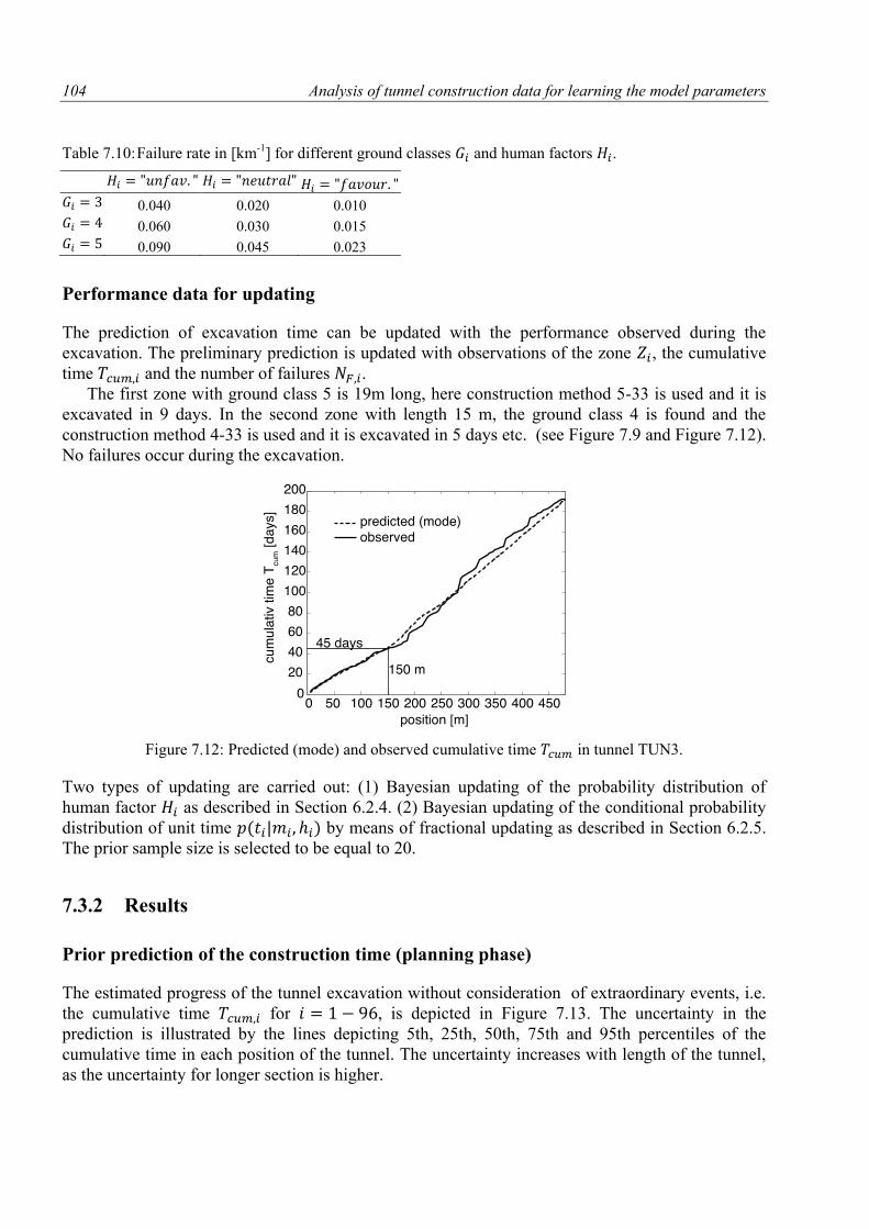
104 Analysis of tunnel construction data for learning the model parameters
Table 7.10: Failure rate in [km-1] for different ground classes and human factors .
0.040 0.020 0.010
0.060 0.030 0.015
0.090 0.045 0.023
Performance data for updating
The prediction of excavation time can be updated with the performance observed during the
excavation. The preliminary prediction is updated with observations of the zone , the cumulative
time and the number of failures .
The first zone with ground class 5 is 19m long, here construction method 5-33 is used and it is
excavated in 9 days. In the second zone with length 15 m, the ground class 4 is found and the
construction method 4-33 is used and it is excavated in 5 days etc. (see Figure 7.9 and Figure 7.12).
No failures occur during the excavation.
Figure 7.12: Predicted (mode) and observed cumulative time in tunnel TUN3.
Two types of updating are carried out: (1) Bayesian updating of the probability distribution of
human factor as described in Section 6.2.4. (2) Bayesian updating of the conditional probability
distribution of unit time | by means of fractional updating as described in Section 6.2.5.
The prior sample size is selected to be equal to 20.
7.3.2 Results
Prior prediction of the construction time (planning phase)
The estimated progress of the tunnel excavation without consideration of extraordinary events, i.e.
the cumulative time for , is depicted in Figure 7.13. The uncertainty in the
prediction is illustrated by the lines depicting 5th, 25th, 50th, 75th and 95th percentiles of the
cumulative time in each position of the tunnel. The uncertainty increases with length of the tunnel,
as the uncertainty for longer section is higher.
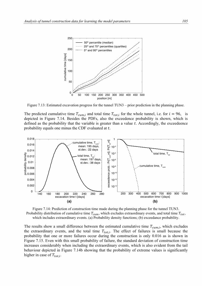
Analysis of tunnel construction data for learning the model parameters 105
Figure 7.13: Estimated excavation progress for the tunnel TUN3 – prior prediction in the planning phase.
The predicted cumulative time and total time for the whole tunnel, i.e. for , is
depicted in Figure 7.14. Besides the PDFs, also the exceedence probability is shown, which is
defined as the probability that the variable is greater than a value . Accordingly, the exceedeence
probability equals one minus the CDF evaluated at
Figure 7.14: Prediction of construction time made during the planning phase for the tunnel TUN3.
Probability distribution of cumulative time , which excludes extraordinary events, and total time ,
which includes extraordinary events. (a) Probability density functions; (b) exceedance probability.
The results show a small difference between the estimated cumulative time , which excludes
the extraordinary events, and the total time . The effect of failures is small because the
probability that one or more failures occur during the construction is only 0.016 as is shown in
Figure 7.15. Even with this small probability of failure, the standard deviation of construction time
increases considerably when including the extraordinary events, which is also evident from the tail
behaviour depicted in Figure 7.14b showing that the probability of extreme values is significantly
higher in case of .
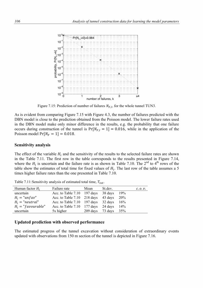
106 Analysis of tunnel construction data for learning the model parameters
Figure 7.15: Prediction of number of failures , for the whole tunnel TUN3.
As is evident from comparing Figure 7.15 with Figure 4.3, the number of failures predicted with the
DBN model is close to the prediction obtained from the Poisson model. The lower failure rates used
in the DBN model make only minor difference in the results, e.g. the probability that one failure
occurs during construction of the tunnel is [ ] , while in the application of the
Poisson model [ ] .
Sensitivity analysis
The effect of the variable and the sensitivity of the results to the selected failure rates are shown
in the Table 7.11. The first row in the table corresponds to the results presented in Figure 7.14,
where the is uncertain and the failure rate is as shown in Table 7.10. The 2nd
to 4th
rows of the
table show the estimates of total time for fixed values of . The last row of the table assumes a 5
times higher failure rates than the one presented in Table 7.10.
Table 7.11: Sensitivity analysis of estimated total time, .
Human factor Failure rate Mean St.dev. uncertain Acc. to Table 7.10 197 days 38 days 19%
Acc. to Table 7.10 218 days 43 days 20%
Acc. to Table 7.10 197 days 32 days 16%
Acc. to Table 7.10 177 days 24 days 14%
uncertain 5x higher 209 days 73 days 35%
Updated prediction with observed performance
The estimated progress of the tunnel excavation without consideration of extraordinary events
updated with observations from 150 m section of the tunnel is depicted in Figure 7.16.
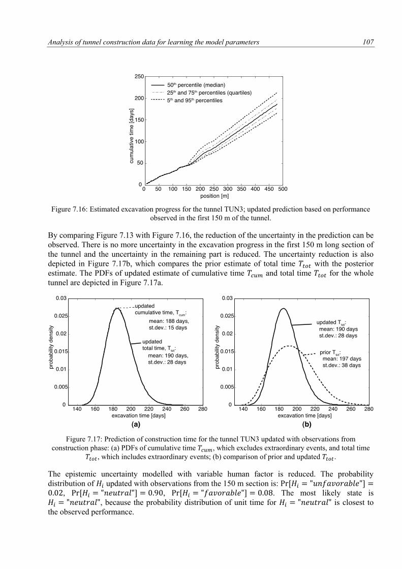
Analysis of tunnel construction data for learning the model parameters 107
Figure 7.16: Estimated excavation progress for the tunnel TUN3; updated prediction based on performance
observed in the first 150 m of the tunnel.
By comparing Figure 7.13 with Figure 7.16, the reduction of the uncertainty in the prediction can be
observed. There is no more uncertainty in the excavation progress in the first 150 m long section of
the tunnel and the uncertainty in the remaining part is reduced. The uncertainty reduction is also
depicted in Figure 7.17b, which compares the prior estimate of total time with the posterior
estimate. The PDFs of updated estimate of cumulative time and total time for the whole
tunnel are depicted in Figure 7.17a.
Figure 7.17: Prediction of construction time for the tunnel TUN3 updated with observations from
construction phase: (a) PDFs of cumulative time , which excludes extraordinary events, and total time
, which includes extraordinary events; (b) comparison of prior and updated .
The epistemic uncertainty modelled with variable human factor is reduced. The probability
distribution of updated with observations from the 150 m section is: [ ] , [ ] , [ ] . The most likely state is
, because the probability distribution of unit time for is closest to
the observed performance.
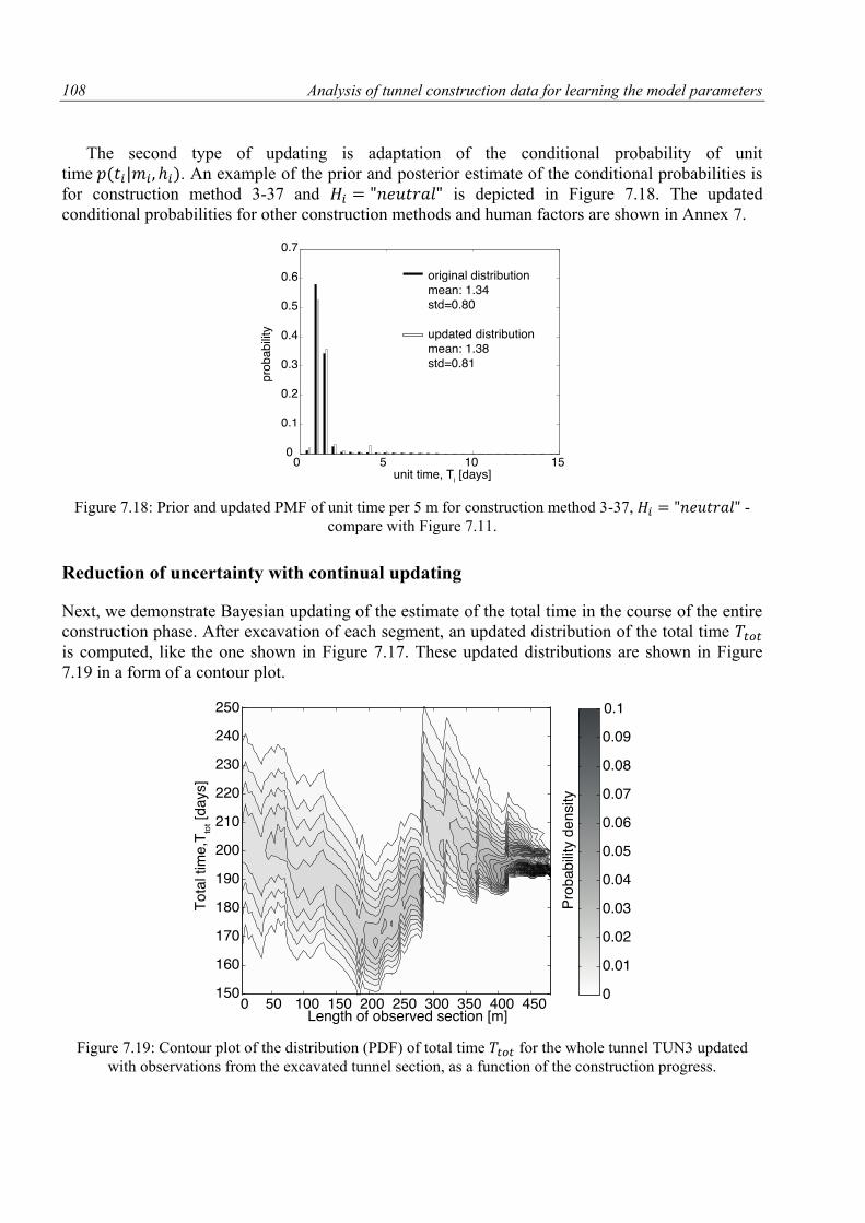
108 Analysis of tunnel construction data for learning the model parameters
The second type of updating is adaptation of the conditional probability of unit
time | . An example of the prior and posterior estimate of the conditional probabilities is
for construction method 3-37 and is depicted in Figure 7.18. The updated
conditional probabilities for other construction methods and human factors are shown in Annex 7.
Figure 7.18: Prior and updated PMF of unit time per 5 m for construction method 3-37, - compare with Figure 7.11.
Reduction of uncertainty with continual updating
Next, we demonstrate Bayesian updating of the estimate of the total time in the course of the entire
construction phase. After excavation of each segment, an updated distribution of the total time
is computed, like the one shown in Figure 7.17. These updated distributions are shown in Figure
7.19 in a form of a contour plot.
Figure 7.19: Contour plot of the distribution (PDF) of total time for the whole tunnel TUN3 updated
with observations from the excavated tunnel section, as a function of the construction progress.
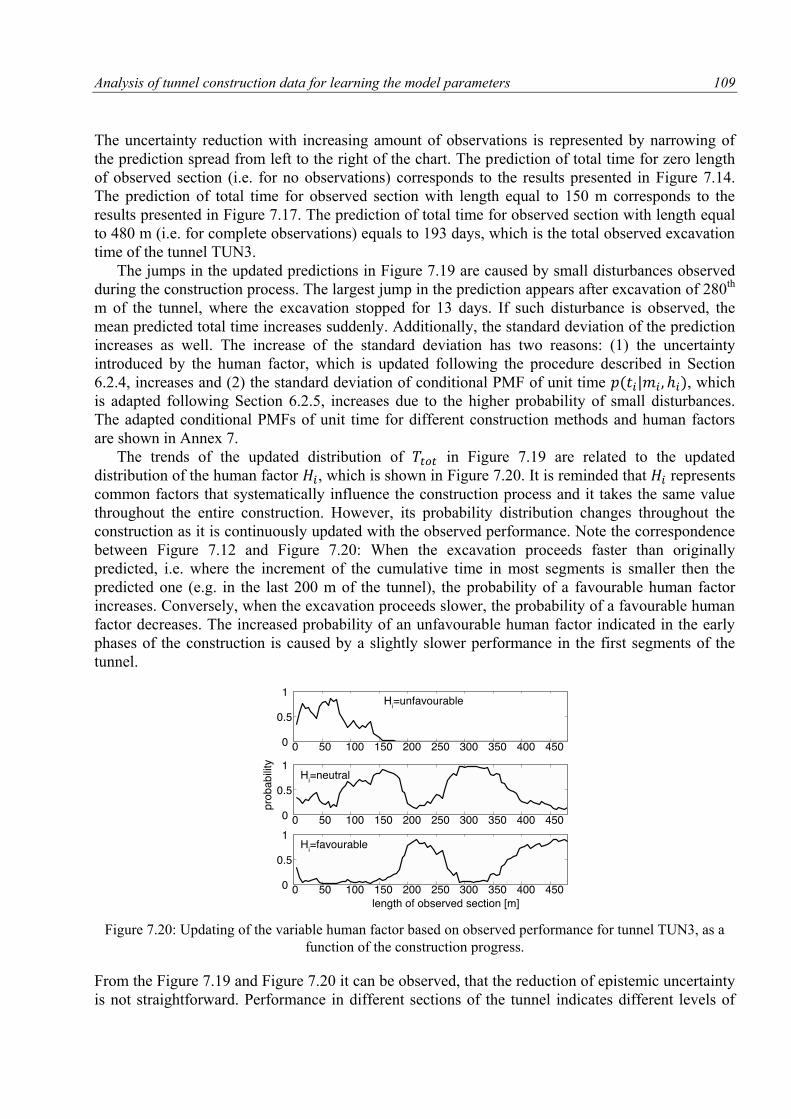
Analysis of tunnel construction data for learning the model parameters 109
The uncertainty reduction with increasing amount of observations is represented by narrowing of
the prediction spread from left to the right of the chart. The prediction of total time for zero length
of observed section (i.e. for no observations) corresponds to the results presented in Figure 7.14.
The prediction of total time for observed section with length equal to 150 m corresponds to the
results presented in Figure 7.17. The prediction of total time for observed section with length equal
to 480 m (i.e. for complete observations) equals to 193 days, which is the total observed excavation
time of the tunnel TUN3.
The jumps in the updated predictions in Figure 7.19 are caused by small disturbances observed
during the construction process. The largest jump in the prediction appears after excavation of 280th
m of the tunnel, where the excavation stopped for 13 days. If such disturbance is observed, the
mean predicted total time increases suddenly. Additionally, the standard deviation of the prediction
increases as well. The increase of the standard deviation has two reasons: (1) the uncertainty
introduced by the human factor, which is updated following the procedure described in Section
6.2.4, increases and (2) the standard deviation of conditional PMF of unit time | , which
is adapted following Section 6.2.5, increases due to the higher probability of small disturbances.
The adapted conditional PMFs of unit time for different construction methods and human factors
are shown in Annex 7.
The trends of the updated distribution of in Figure 7.19 are related to the updated
distribution of the human factor , which is shown in Figure 7.20. It is reminded that represents
common factors that systematically influence the construction process and it takes the same value
throughout the entire construction. However, its probability distribution changes throughout the
construction as it is continuously updated with the observed performance. Note the correspondence
between Figure 7.12 and Figure 7.20: When the excavation proceeds faster than originally
predicted, i.e. where the increment of the cumulative time in most segments is smaller then the
predicted one (e.g. in the last 200 m of the tunnel), the probability of a favourable human factor
increases. Conversely, when the excavation proceeds slower, the probability of a favourable human
factor decreases. The increased probability of an unfavourable human factor indicated in the early
phases of the construction is caused by a slightly slower performance in the first segments of the
tunnel.
Figure 7.20: Updating of the variable human factor based on observed performance for tunnel TUN3, as a
function of the construction progress.
From the Figure 7.19 and Figure 7.20 it can be observed, that the reduction of epistemic uncertainty
is not straightforward. Performance in different sections of the tunnel indicates different levels of
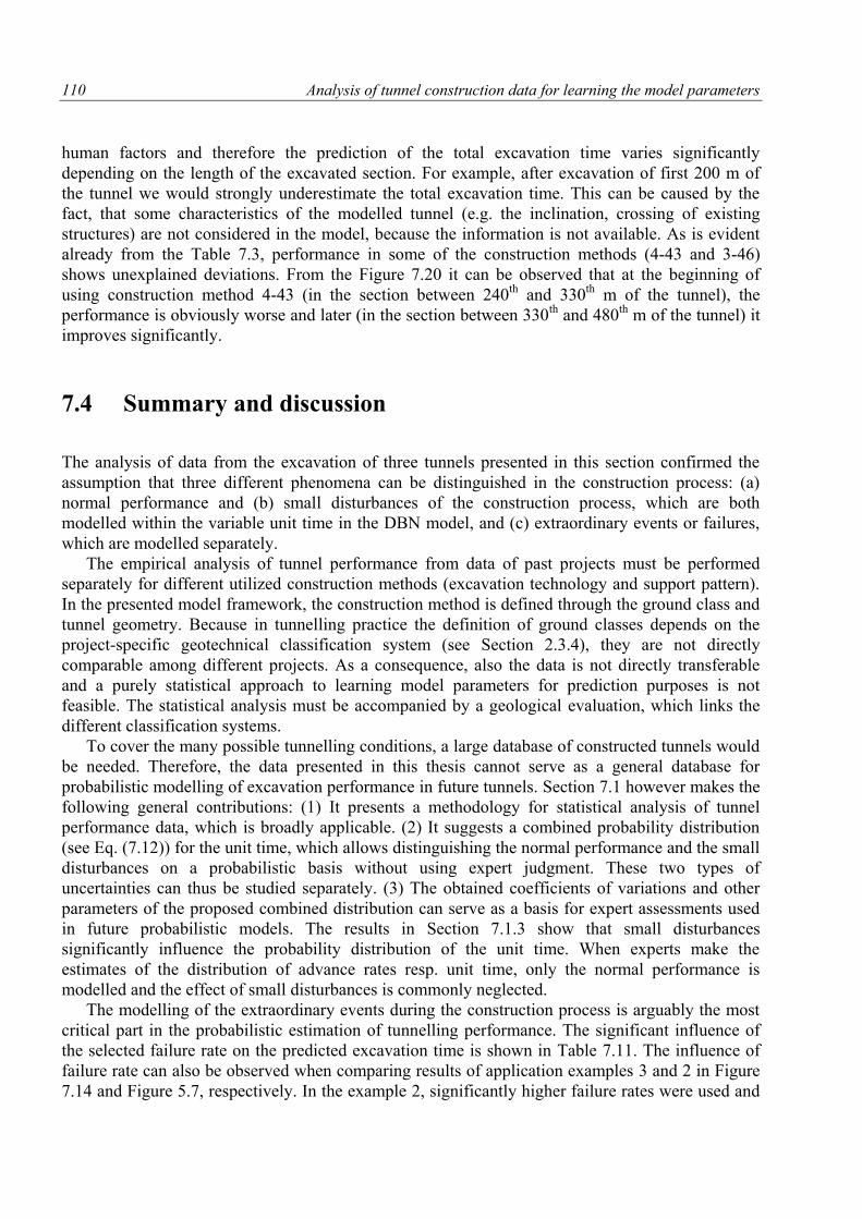
110 Analysis of tunnel construction data for learning the model parameters
human factors and therefore the prediction of the total excavation time varies significantly
depending on the length of the excavated section. For example, after excavation of first 200 m of
the tunnel we would strongly underestimate the total excavation time. This can be caused by the
fact, that some characteristics of the modelled tunnel (e.g. the inclination, crossing of existing
structures) are not considered in the model, because the information is not available. As is evident
already from the Table 7.3, performance in some of the construction methods (4-43 and 3-46)
shows unexplained deviations. From the Figure 7.20 it can be observed that at the beginning of
using construction method 4-43 (in the section between 240th
and 330th
m of the tunnel), the
performance is obviously worse and later (in the section between 330th
and 480th
m of the tunnel) it
improves significantly.
7.4 Summary and discussion
The analysis of data from the excavation of three tunnels presented in this section confirmed the
assumption that three different phenomena can be distinguished in the construction process: (a)
normal performance and (b) small disturbances of the construction process, which are both
modelled within the variable unit time in the DBN model, and (c) extraordinary events or failures,
which are modelled separately.
The empirical analysis of tunnel performance from data of past projects must be performed
separately for different utilized construction methods (excavation technology and support pattern).
In the presented model framework, the construction method is defined through the ground class and
tunnel geometry. Because in tunnelling practice the definition of ground classes depends on the
project-specific geotechnical classification system (see Section 2.3.4), they are not directly
comparable among different projects. As a consequence, also the data is not directly transferable
and a purely statistical approach to learning model parameters for prediction purposes is not
feasible. The statistical analysis must be accompanied by a geological evaluation, which links the
different classification systems.
To cover the many possible tunnelling conditions, a large database of constructed tunnels would
be needed. Therefore, the data presented in this thesis cannot serve as a general database for
probabilistic modelling of excavation performance in future tunnels. Section 7.1 however makes the
following general contributions: (1) It presents a methodology for statistical analysis of tunnel
performance data, which is broadly applicable. (2) It suggests a combined probability distribution
(see Eq. (7.12)) for the unit time, which allows distinguishing the normal performance and the small
disturbances on a probabilistic basis without using expert judgment. These two types of
uncertainties can thus be studied separately. (3) The obtained coefficients of variations and other
parameters of the proposed combined distribution can serve as a basis for expert assessments used
in future probabilistic models. The results in Section 7.1.3 show that small disturbances
significantly influence the probability distribution of the unit time. When experts make the
estimates of the distribution of advance rates resp. unit time, only the normal performance is
modelled and the effect of small disturbances is commonly neglected.
The modelling of the extraordinary events during the construction process is arguably the most
critical part in the probabilistic estimation of tunnelling performance. The significant influence of
the selected failure rate on the predicted excavation time is shown in Table 7.11. The influence of
failure rate can also be observed when comparing results of application examples 3 and 2 in Figure
7.14 and Figure 5.7, respectively. In the example 2, significantly higher failure rates were used and
Analysis of tunnel construction data for learning the model parameters 111
the resulting estimate of total time is thus strongly skewed. The failure rate has not been studied
systematically in the past and cannot be assessed reliably from the available data, as discussed in
Section 7.2.2. At present, available databases collect detailed information on selected observed
extraordinary events. However, for the purpose of estimating failure rates, records of all
extraordinary events within a sample of tunnels would be needed. Such a sample could e.g. be all
tunnels of a certain type in a specific region and time period. Ideally, additional information on
geotechnical conditions and construction method should also be available in such a database. When
modelling a specific tunnel construction, the statistical estimate of the failure rate should be
accompanied by expert estimates and/or structural reliability analysis.
The utilization of the resulting statistical models for the probabilistic prediction of tunnel
construction time using a DBN model is illustrated in the application example of Section 7.3. For
the prior prediction during the design phase, the parameters of the DBN model are determined by
expert assessments informed by the available data. During the construction, the prior prediction is
updated using observed performance data. A significant part of the prior uncertainty is due to the
epistemic uncertainty modelled by the random variable human factor, which represents the
deviation of the actual performance from the mean predicted performance. In the present model,
this human factor is assumed to take on one value during the entire construction. The results of the
case study indicate that a more refined model, which allows for different values of the human factor
for different construction methods, might be more accurate. In spite of this, the results show that the
proposed model enables learning during the construction process.
-

113
The construction time and cost in infrastructure projects are systematically underestimated. A main
reason for this underestimation is the fact that the uncertainty of the estimates is not considered in
the planning of the projects and estimators are asked to provide deterministic values. Because of
psychological and political reasons, they tend to estimate the construction time and costs too
optimistically. However, even if the estimators would provide correct expected values of the
construction time and cost, such estimates might not be sufficient for making optimal decisions,
because the decision should also reflect the attitude of the decision maker to risk.
In current practice, the project risks are commonly analysed on a qualitative basis. Qualitative
analysis is an irreplaceable basis for prioritizing the hazards and risks, for development of risk
treatment strategies and for allocating the responsibilities. The identification of hazards carried out
during the qualitative analysis is a basis for risk quantification. However, direct use of risk registers
for assessment of the overall risk, which is often applied in the practice, is incorrect. The risk
registers do not take into account the interconnectivity and dependences amongst different hazards.
They therefore cannot provide a correct numerical estimate of the overall risk.
To make the investments to the infrastructure more effective, it is thus needed to change the
present practice and to estimate the construction time and costs on a probabilistic basis. The model
for such estimation must realistically assess the uncertainties influencing the construction process,
the assumptions and logic of the model must be understandable and transparent, the inputs of the
model should be based on analysis of data from past projects and the evaluation must be efficient
enough in order to be utilizable for real-time management of the construction process.
This thesis is a step towards realistic quantification of construction risk. It presents two models
for probabilistic prediction of tunnel construction time: a simple model for estimating delay of the
tunnel construction due to failures using Poisson process and Event Tree Analysis (Chapter 4) and
an advanced model using Dynamic Bayesian Networks (Chapter 5). The models consider the
common factors (e.g. quality of planning, organization of the construction works), which
systematically influence the construction performance, and the epistemic uncertainty, i.e. the
uncertainty in the expected construction progress due to incomplete knowledge the estimator has in
8 Conclusions and outlook
114 Tunnel projects and risk management
the planning phase. The DBN model allows taking into account the uncertainties in geotechnical
conditions and the common variability of excavation performance. Further, it allows updating of the
predictions based on excavation performance observed after the construction commences. The
utilization of the models is demonstrated by three applications examples.
The use of the probabilistic estimation of construction time for the risk assessment and decision-
making is illustrated in Chapter 4, taking into account the risk perception of the decision-maker by
means of a utility function. Two alternative tunnelling technologies are evaluated based on
comparison of the associated risk and costs. It is shown that including the risk aversion of the
decision-maker changes the decision; the risk aversion of the contractor outweighs the benefits from
the cost savings.
A methodology for statistical analysis of excavation performance data is shown in Chapter 7
using data from three tunnels built with conventional tunnelling method. The results show that three
types of phenomena can be observed in the construction performance: (1) the normal performance,
(2) small disturbances of the construction process, (3) the extraordinary events. All of these
phenomena have a significant impact on the estimate of the construction time. Expert estimates
based on such statistical analyses are more likely to realistically appraise the effects of small
disturbances and extraordinary events on the total construction time.
An algorithm for the efficient evaluation of the DBN is described in Chapter 6. The existing
Frontier algorithm was modified to better address specific features of the proposed DBN. The
modification enables one to deal with discrete random variables with the large numbers of
outcomes states that result from the discretization of continuous random variables such as time or
cost. We exploit the fact that these variables are defined as cumulative sums of other random
variables in the DBN and that the probability distribution of a sum of two random variables can be
efficiently calculated by means of convolution.
8.1 Main contributions of the thesis
This thesis had two main objectives (see Section 1.1): to develop probabilistic models for realistic
estimate of tunnel construction time (costs) and to analyse the performance data from the tunnels
constructed in the past. The thesis focuses on quantitative analysis of the uncertainties. Compared to
previous works carried out in this field, the thesis makes the following new contributions:
A simple model for the probabilistic estimation of the delay due to tunnel construction failures (e.g. cave-in collapses) is proposed. It can be used in conjunction with a deterministic estimate of the construction time. The model has the following new features:
It takes into account the uncertainty in the estimates of the failure consequences. By now, the consequences of the construction failures were commonly represented by their mean values or they were evaluated qualitatively.
The model takes into account the variability of the failure rate in different sections of the tunnel; the failure rate changes with the changing geotechnical conditions along the tunnel axis.
The model includes the epistemic uncertainty in the estimation of the failure rate.
The model framework enables learning the model parameters from data. The logic of the model is analogous with modelling of failures in the complex DBN model, the parameter estimations are thus valid for both models.
115
An advanced DBN model was proposed including both types of uncertainties, i.e. the common variability of the construction performance and extraordinary events (failures). Compared to existing models it has the following main advantages:
It includes the epistemic uncertainty which reflects the fact that the applied probabilistic models of the construction performance are uncertain. The uncertainty is caused above all by the unknown effect of human and other external factors. These factors cause strong correlation among the performance at different phases of the construction. The inclusion of the epistemic uncertainty leads to an increased variance of the estimate of construction time.
The proposed DBN approach is flexible with regard to the changes in the model. Modelling of geotechnical conditions can be adjusted depending on the specific conditions of the tunnel; the modelling of construction performance can be modified for other tunnelling technologies or even for other infrastructures.
The DBN model allows for an efficient updating of the predictions with additional observations.
The graphical nature of DBN strongly facilitates the representation and communication of the model assumptions.
The results of the model demonstrated in two application examples seem to realistically reflect the uncertainties of the construction time estimates.
An efficient algorithm for evaluating the DBN model is proposed. The algorithm can be used in various applications of DBN models which include random variables that are defined as sums of other random variables in the DBN.
The analysis of data from previous projects makes the following contributions:
A methodology for statistical analysis of tunnel performance data is presented which is broadly applicable also to other types of linear infrastructure.
It is shown that the commonly used probabilistic models of variability of unit time (activity duration), i.e. the triangular, beta or lognormal distributions, are likely to miss an important part of the uncertainty - the small disturbances of the construction process.
A novel combined distribution for representing the unit time is therefore proposed. It allows distinguishing the normal performance and the small disturbances on a probabilistic basis without using expert judgment.
Data from available databases of world tunnels and tunnel failures are analysed. The analysis gives a rough indication of the construction failure rates. Hitherto, such analysis was not available in the literature.
The delays of tunnel construction due to occurrence of failures are studied statistically using data from an existing database. A shifted exponential distribution seems to accurately describe the delay.
An overview of tunnels and tunnel construction failures in the Czech republic since 1990 is collected. These data were missing in all the available databases of tunnel failures.
8.2 Outlook
The presented thesis addresses just a part of the problem of optimization of the decisions in
infrastructure projects. Further research and work is needed before the new concept can be applied
116 Tunnel projects and risk management
in the practice. Additionally, the proposed models may require improvements in the future.
Limitations of the presented work and directions for future research are discussed in the following:
The models presented in this thesis are applied to estimate the tunnel construction time; the construction costs are discussed only briefly. The construction costs might be assessed using the DBN model by replacing the time variables with cost variables. This approach, which is used in many existing models, is however likely to oversimplify the reality. The costs, or at least a significant part of them (labour costs, machinery costs), are strongly time dependent. They should therefore be modelled as a function of the construction time. Further investigations in the field of construction costs are needed. However, this research might be hindered by the sensitivity of the cost information and by the complicated system of cost monitoring and control.
The presented DBN model neglects additional time (costs) needed when changing construction methods and the influence of this additional time on the decisions on changes (see Section 5.1.2). This omission is not critical in the presented applications, because ground classes and the corresponding construction methods do not change frequently. However, this factor should be included in the future.
In the present DBN model, the epistemic uncertainty is modelled by one random variable (called human factor), which is fully correlated through the whole construction process. The results of the last application example (Section 7.3.2) indicate that a more refined model, which allows for different values of the human factor for different construction methods, might be more accurate.
Performance data from three completed tunnels were analysed in this thesis. For making predictions in future tunnels, establishment of a much bigger database covering the whole variety of the tunnels is needed. The tunnels in the database should be categorized depending on the geotechnical conditions, type and geometry, construction technology and other factors, which influence the construction performance. Concurrently, it is necessary to make links between the geotechnical classification systems used in different projects.
The modelling of the extraordinary events during the construction process is a critical part in the probabilistic estimation of tunnelling performance. The failure rate has not been studied systematically in the past and cannot be assessed reliably from available data, as discussed in Section 7.2.2. At present, available databases collect detailed information on selected observed extraordinary events. However, for the purpose of estimating failure rates, records of all extraordinary events within a sample of tunnels would be needed. Such a sample could, e.g., be all tunnels of a certain type in a specific region and time period. Ideally, additional information on geotechnical conditions and construction method should also be available in such a database. When modelling a specific tunnel construction, the statistical estimate of the failure rate should be accompanied by expert estimates and/or structural reliability analysis.
The understanding of the benefits of probabilistic modelling among stakeholders should be raised which should lead them to more systematically manage and statistically analyse data from available projects.
Application of the proposed models to mechanized tunnelling eventually to other types of linear infrastructure (roads, railways etc.) should be investigated.
To make full use of the probabilistic estimates of construction time and costs in the project planning and management, the topic of decision making under uncertainty must be further developed. This thesis only briefly mentions the concept of utility theory (Section 3.3.7) and gives a simple example of the risk quantification and decision-making (Section 4.2). To realistically capture the whole complexity of the problem, the application of the utility theory in infrastructure projects should be further investigated. The decision concept should allow taking into account both measurable criteria, such as construction time and cost or maintenance costs, and soft criteria such as environmental or social impacts.
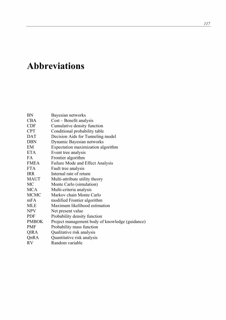
117
BN Bayesian networks
CBA Cost – Benefit analysis
CDF Cumulative density function
CPT Conditional probability table
DAT Decision Aids for Tunneling model
DBN Dynamic Bayesian networks
EM Expectation maximization algorithm
ETA Event tree analysis
FA Frontier algorithm
FMEA Failure Mode and Effect Analysis
FTA Fault tree analysis
IRR Internal rate of return
MAUT Multi-attribute utility theory
MC Monte Carlo (simulation)
MCA Multi-criteria analysis
MCMC Markov chain Monte Carlo
mFA modified Frontier algorithm
MLE Maximum likelihood estimation
NPV Net present value
PDF Probability density function
PMBOK Project management body of knowledge (guidance)
PMF Probability mass function
QlRA Qualitative risk analysis
QnRA Quantitative risk analysis
RV Random variable
Abbreviations

119
Abdelgawad, M., Fayek, A.R., 2010. Risk Management in the Construction Industry Using
Combined Fuzzy FMEA and Fuzzy AHP. Journal of Construction Engineering and Management
136, 1028.
AbouRizk, S.M., Ruwanpura, J.Y., Er, K.C., Fernando, S., 1999. Special purpose simulation
template for utility tunnel construction, in: Proceedings of the 31st Conference on Winter
Simulation: Simulation—a Bridge to the Future - Volume 2, WSC ’99. ACM, New York, NY,
USA, pp. 948–955.
Aliahmadi, A., Sadjadi, S., Jafari-Eskandari, M., 2011. Design a new intelligence expert decision
making using game theory and fuzzy AHP to risk management in design, construction, and
operation of tunnel projects (case studies: Resalat tunnel). The International Journal of Advanced
Manufacturing Technology 53, 789–798.
Allianz Insurence, n.d. Insurance for building works including options to insure advanced business
interruption & public liability.
Association of British Insurers (ABI), British Tunnelling Society (BTS), 2003. The joint code of
practice for risk management of tunnel works in the UK.
Aydin, A., 2004. Fuzzy set approaches to classification of rock masses. Engineering Geology 74,
227–245.
Aziz, A.M.A., 2007. Successful delivery of Public-Private Partnerships for infrastructure
development. Journal of Construction Engineering and Management 133, 918–930.
Banister, D., Berechman, J., 2000. Transport investment and economic development. Routledge.
Barták, J., 2007. Underground construction in the Czech Republic. SATRA.
Barták, J., Makásek, P., 2011. Stability Time of the Unsupported Tunnel Excavation. Presented at
the 39. konference zakládání staveb, Brno, pp. 162–168.
Barton, N., Grimstad, E., Aas, G., Opsahl, O.A., Bakken, A., Pedersen, L., Johansen, E.D., 1992.
Norwegian Method of Tunnelling, in: WT Focus on Norway, Worls Tunnelling.
Bibliography
120 Bibliography
Barton, N., Lien, R., Lunde, J., 1974. Engineering classification of rock masses for the design of
tunnel support. Rock Mechanics 6, 189–236.
Benardos, A.G., Kaliampakos, D.C., 2004. Modelling TBM performance with artificial neural
networks. Tunnelling and Underground Space Technology 19, 597–605.
Benjamin, J.R., Cornell, C.A., 1970. Probability, statistics, and decision for civil engineers.
McGraw-Hill.
Bieniawski, Z.T., 1989. Engineering rock mass classifications: a complete manual for engineers and
geologists in mining, civil, and petroleum engineering. Wiley-Interscience.
Blockley, D., 1999. Risk based structural safety methods in context. Structural Safety 21, 335–348.
Burbaum, U., Krajewski, W., Seeger, K.J., 2005. Wirtschaftliche Aspekte bei Tunnelbauwerken in
fr hen Planungsphasen. Hessische Stra en- und Verkehrsverwaltung.
Castillo, E., Menéndez, J.M., Sánchez-Cambronero, S., 2008. Predicting traffic flow using Bayesian
networks. Transportation Research Part B: Methodological 42, 482–509.
Chakraborty, P.P., Mukhopadhyay, B., Pal, T., Dutta, G.T., 2002. Statistical appraisal of bed
thickness patterns in turbidite successions, Andaman Flysch Group, Andaman Islands, India.
Journal of Asian Earth Sciences 21, 189–196.
Chan, M.H.C., 1981. A geological prediction and updating model in tunneling (Thesis).
Cheung, S.H., Beck, J.L., 2010. Calculation of Posterior Probabilities for Bayesian Model Class
Assessment and Averaging from Posterior Samples Based on Dynamic System Data. Computer
Aided Civil and Infrastructure Engineering 25, 304–321.
Chou, J.-S., 2011. Cost simulation in an item-based project involving construction engineering and
management. International Journal of Project Management 29, 706–717.
Chung, T.H., Mohamed, Y., AbouRizk, S., 2006. Bayesian Updating Application into Simulation in
the North Edmonton Sanitary Trunk Tunnel Project. Journal of Construction Engineering and
Management 132, 882–894.
Clayton, C.R.I., 2001. Managing Geotechnical Risk: Improving Productivity in UK Building and
Construction. Thomas Telford Ltd.
Cooke, R., Jager, E., 1998. A Probabilistic Model for the Failure Frequency of Underground Gas
Pipelines. Risk Analysis, Risk Analysis 18, 18, 511, 511–527, 527.
Cornell, C.A., 1968. Engineering Seismic Risk Analysis. Bulletin of the Seismological Society of
America 58, 1583–1606.
Deere, D.U., Deere, D.W., 1988. The Rock Quality Designation (RQD) index in practice, in:
Kirkaldie, L. (Ed.), Rock Classification Systems for Engineering Purposes. Presented at the
Symposium on rock classification systems for engineering purposes, American society for testing
and materials, Cincinnati, Ohio.
Bibliography 121
Department for Communities and Local Government, 2009. Multi-criteria analysis: a manual.
Der Kiureghian, A., Ditlevsen, O., 2009. Aleatory or epistemic? Does it matter? Structural Safety
31, 105–112.
Ditlevsen, O., 2006. A story about distributions of dimensions and locations of boulders.
Probabilistic Engineering Mechanics 21, 9–17.
Dozzi, S.P., AbouRizk, S.M., Schroeder, S.L., 1996. Utility-Theory Model for Bid Markup
Decisions. Journal of Construction Engineering and Management 122, 119–124.
Edgerton, W.W., 2008. Recommended Contract Practices for Underground Construction. SME.
Edwards, L., 1995. Practical risk management in the construction industry. Thomas Telford.
Einstein, H.H., 1996. Risk and risk analysis in rock engineering. Tunnelling and Underground
Space Technology 11, 141–155.
Elishakoff, I., 1999. Probabilistic Theory of Structures. Dover Publications.
Ericson, C.A., 2005. Hazard Analysis Techniques for System Safety. John Wiley & Sons.
Eskesen, D.S., Tengborg, P., Kampmann, J., Veicherts, H.T., 2004. Guidelines for tunnelling risk
management: International Tunnelling Association, Working Group No. 2. Tunnelling and
Underground Space Technology 19, 217–237.
Faber, M.H., Kroon, I.B., Kragh, E., Bayly, D., Decosemaeker, P., 2002. Risk Assessment of
Decommissioning Options Using Bayesian Networks. J. Offshore Mech. Arct. Eng. 124, 231–238.
Farrokh, E., Rostami, J., Laughton, C., 2012. Study of various models for estimation of penetration
rate of hard rock TBMs. Tunnelling and Underground Space Technology.
Felletti, F., Bersezio, R., 2010. Quantification of the degree of confinement of a turbidite-filled
basin: A statistical approach based on bed thickness distribution. Marine and Petroleum Geology
27, 515–532.
Flanagan, R., Jewell, C., 2005. Whole Life Appraisal: for Construction, 1st ed. Wiley-Blackwell.
Flanagan, R., Norman, G., 1993. Risk Management and Construction, 1st ed. Wiley-Blackwell.
Flyvbjerg, B., 2006. From Nobel prize to project management: getting risks right. Project
Management Journal 37, 5.
Flyvbjerg, B., COWI, 2004. Procedures for Dealing with Optimism Bias in Transport Planning,
Guidance document of The British Department for Transport ( No. 58924).
Flyvbjerg, B., Holm, S.M.K., Buhl, S.L., 2002. Underestimating Costs in Public Works Projects:
Error or Lie? Journal of the American Planning Association, 68, 279–295.
122 Bibliography
Fulvio, T., 2010. Sequential excavation, NATM and ADECO: What they have in common and how
they differ. Tunnelling and Underground Space Technology 25, 245–265.
Ge, M., Du, R., Xu, Y., 2004. Hidden Markov Model based fault diagnosis for stamping processes.
Mechanical Systems and Signal Processing 18, 391–408.
Gilks, W.R., Richardson, S., Spiegelhalter, D.J., 1996. Markov chain Monte Carlo in practice.
Chapman & Hall.
Goel, R.K., Jethwa, J.L., Paithankar, A.G., 1996. Correlation between Barton’s Q and Bieniawski’s
RMR—A new approach. International Journal of Rock Mechanics and Mining Sciences &
Geomechanics Abstracts 33, 179–181.
Goodwin, P., Wright, G., 2010. The limits of forecasting methods in anticipating rare events.
Technological Forecasting and Social Change 77, 355–368.
Grasso, P., Xu, S., Pescara, M., Russo, G., Repetto, L., 2006. A Methodology for the Geotechnical
Design of Long High-Speed Rail Tunnels Under the Conditions of Uncertainty. Presented at the
China International Symposium on HighSpeed Railway Tunnels Exhibition, Beijing, China.
Grêt-Regamey, A., Straub, D., 2006. Spatially explicit avalanche risk assessment linking Bayesian
networks to a GIS. Nat. Hazards Earth Syst. Sci. 6, 911–926.
Grinstead, C.M., Snell, J.L., 1997. Introduction to Probability. American Mathematical Soc.
Haas, C., Einstein, H.H., 2002. Updating the Decision Aids for Tunneling. Journal of Construction
Engineering and Management 128, 40–48.
Henning, J.E., Melby, K., Øvstedal, E., Amundsen, F.H., Ranes, G., 2007. Experiences with subsea
road tunnels in Norway-construction, operation, costs and maintenance. Chinese Journal of Rock
Mechanics and Engineering 26, 2226–2235.
HM Treasury, 2003. The Green Book: Appraisal and Evaluation in Central Government.
Hong, E.-S., Lee, I.-M., Shin, H.-S., Nam, S.-W., Kong, J.-S., 2009. Quantitative risk evaluation
based on event tree analysis technique: Application to the design of shield TBM. Tunnelling and
Underground Space Technology 24, 269–277.
HSE (Health & Safety Executive), 1996. Safety of New Austrian Tunnelling Method (NATM)
tunnels: a review of sprayed concrete lined tunnels with particular reference to London clay. Health
& Safety Executive, Sudbury, UK.
HSE (Health & Safety Executive), 2006. The risk to third parties from bored tunnelling in soft
ground – research report 453. Health & Safety Executive, HSE Books, Sudbury, Suffolk, GB.
Hu, J., Zhang, L., Ma, L., Liang, W., 2011. An integrated safety prognosis model for complex
system based on dynamic Bayesian network and ant colony algorithm. Expert Systems with
Applications 38, 1431–1446.
Bibliography 123
IMIA (The International Association of Engineering Insurers), 2006. ALOP/DSU coverage for
tunnelling risks? Presented at the The International Association of Engineering Insurers 39th
Annual Conference, Boston.
Institution of Civil Engineers, Faculty of Actuaries, Institute of Actuaries, 2005. RAMP - risk
analysis and management for projects: a strategic framework for managing project risk and its
financial implications. Thomas Telford.
International Transport Forum, OECD, 2011. Trends in transport infrastructure investment 1995-
2009. OECD.
Isaksson, T., 2002. Model for estimation of time and cost based on risk evaluation applied on tunnel
projects (Doctoral thesis).
Isaksson, T., Stille, H., 2005. Model for Estimation of Time and Cost for Tunnel Projects Based on
Risk Evaluation. Rock Mechanics and Rock Engineering 38, 373–398.
ISO - International Organization for Standardization, 2009. ISO 31000:2009 Risk management --
Principles and guidelines (Text).
ITA (International Tunnelling Association), 2001. Recommendations and Guidelines for Tunnel
Boring Machines (TBMs).
ITA (International Tunnelling Association), 2009. General report on conventional tunnelling
method ( No. 002).
ITIG (International Tunnelling Insurance Group), 2006. A code of practice for risk management of
tunnel works.
Jensen, F.V., Nielsen, T.D., 2007. Bayesian networks and decision graphs. Springer.
Jimenez, J.M., 1999. Feasibility of the SIMSUPER simulation model in the renovation of building
projects.
Jordaan, I.J., 2005. Decisions Under Uncertainty: Probabilistic Analysis for Engineering Decisions.
Cambridge University Press.
Jurado, A., De Gaspari, F., Vilarrasa, V., Bolster, D., Sánchez-Vila, X., Fernàndez-Garcia, D.,
Tartakovsky, D.M., 2012. Probabilistic analysis of groundwater-related risks at subsurface
excavation sites. Engineering Geology 125, 35–44.
Karakus, M., Fowell, R.J., 2004. An insight into the New Austrian Tunnelling Method (NATM).
Presented at the ROCKMEC′2004-VIIth Regional Rock Mechanics Symposium, Sivas, Turkey.
Keeney, R.L., Raiffa, H., 1993. Decisions with Multiple Objectives: Preferences and Value
Tradeoffs. Cambridge University Press.
Khakzad, N., Khan, F., Amyotte, P., 2011. Safety analysis in process facilities: Comparison of fault
tree and Bayesian network approaches. Reliability Engineering & System Safety 96, 925–932.
124 Bibliography
Kim, Y., Bruland, A., 2009. Effect of rock mass quality on construction time in a road tunnel.
Tunnelling and Underground Space Technology 24, 584–591.
Kobayashi, K., Kaito, K., Lethanh, N., 2012. A statistical deterioration forecasting method using
hidden Markov model for infrastructure management. Transportation Research Part B:
Methodological 46, 544–561.
Koski, T., Noble, J.M., 2009. Bayesian networks: an introduction. John Wiley and Sons.
Kottegoda, N.T., Rosso, R., 2008. Applied statistics for civil and environmental engineers.
Blackwell Publishing.
Laderian, A., Abaspoor, M.A., 2012. The correlation between RMR and Q systems in parts of Iran.
Tunnelling and Underground Space Technology 27, 149–158.
Lædre, O., Austeng, K., Haugen, T.I., Klakegg, O.J., 2006. Procurement Routes in Public Building
and Construction Projects. Journal of Construction Engineering and Management 132, 689–696.
Lambropoulos, 2007. The use of time and cost utility for construction contract award under
European Union Legislation. Building and Environment 42, 452–463.
Landrin, H., Bl ckert, C., Perrin, J.-P., Stacey, S., Stolfa, A., 2006. ALOP/DSU coverage for
tunnelling risks? Presented at the 39th Annual Conference, Boston.
Langseth, H., Nielsen, T.D., Rumí, R., Salmerón, A., 2009. Inference in hybrid Bayesian networks.
Reliability Engineering & System Safety 94, 1499–1509.
Lauffer, H., 1958. Gebirgsklassifizierung für den Stollenbau. Geol. Bauwesen 1, 46–51.
Lee Jr., D.., 2000. Methods for evaluation of transportation projects in the USA. Transport Policy 7,
41–50.
Li, B., Akintoye, A., Edwards, P.J., Hardcastle, C., 2005. Critical success factors for PPP/PFI
projects in the UK construction industry. Construction Management and Economics 23, 459–471.
Lin, S.-W., Bier, V.M., 2008. A study of expert overconfidence. Reliability Engineering & System
Safety 93, 711–721.
Lombardi, G., 2001. Geotechnical risks for project financing of tunnels in non-urban areas. Tribune
No 20 – International Tunnelling Association newsletter.
Longhitano, S.G., Nemec, W., 2005. Statistical analysis of bed-thickness variation in a Tortonian
succession of biocalcarenitic tidal dunes, Amantea Basin, Calabria, southern Italy. Sedimentary
Geology 179, 195–224.
Love, P.E.D., Skitmore, M., Earl, G., 1998. Selecting a suitable procurement method for a building
project. Construction Management & Economics 16, 221–233.
Mahboob, Q., Straub, D., 2011. Comparison of fault tree and Bayesian Networks for modeling
safety critical components in railway systems, in: Advances in Safety, Reliability and Risk
Bibliography 125
Management. Presented at the European Safety and Reliability Conference: Advances in Safety,
Reliability and Risk Management, ESREL 2011, Troyes, pp. 89–95.
Melchers, R.E., 1987. Structural reliability: analysis and prediction. Ellis Horwood.
Min, S., 2003. The application of “Decision Aids for Tunneling (DAT)” to the Sucheon tunnel in
Korea (Master thesis, MIT, Boston).
Min, S., 2008. Development of the resource model for the Decision Aids for Tunneling (DAT)
(Doctoral thesis, MIT, Boston).
Min, S., Kim, T.K., Lee, J.S., Einstein, H.H., 2008. Design and construction of a road tunnel in
Korea including application of the Decision Aids for Tunneling – A case study. Tunnelling and
Underground Space Technology 23, 91–102.
Min, S.Y., Einstein, H.H., Lee, J.S., Kim, T.K., 2003. Application of Decision Aids for Tunneling
(DAT) to a drill & blast tunnel. KSCE Journal of Civil Engineering 7, 619–628.
Minka, T.P., 2001. A family of algorithms for approximate Bayesian inference.
Moret, Y., 2011. Modeling cost and time uncertainty in rail line construction (Thesis).
Moret, Y., Einstein, H.H., 2011a. Experience in Expert Estimation of Probabilities and Correlations
for Rail Line Construction. Journal of Construction Engineering and Management 1, 374–374.
Moret, Y., Einstein, H.H., 2011b. Cost and time correlations in linear infrastructure construction, in:
Applications of Statistics and Probability in Civil Engineering. Presented at the ICASP, Zürich, pp.
788–796.
Morisugi, H., 2000. Evaluation methodologies of transportation projects in Japan. Transport Policy
7, 35–40.
Murphy, K.P., 2002. Dynamic Bayesian Networks Representation, Inference and Learning
(Doctoral thesis, Univ. of California, Berkeley.).
Neapolitan, R.E., 2004. Learning Bayesian networks. Pearson Prentice Hall.
Neil, M., Tailor, M., Marquez, D., Fenton, N., Hearty, P., 2008. Modelling dependable systems
using hybrid Bayesian networks. Reliability Engineering & System Safety 93, 933–939.
Nishijima, K., 2009. Issues of sustainability in engineering decision analysis (Thesis).
OECD, 2007. Infrastructure to 2030. Volume 2: Mapping policy for electricity, water and transport.
Ökmen, Ö., Öztaş, A., 2008. Construction Project Network Evaluation with Correlated Schedule
Risk Analysis Model. Journal of Construction Engineering and Management 134, 49–63.
ÖNORM B 2203 - Untertagebauarbeiten - Werkvertragsnorm, n.d. Austrian Standards plus GmbH,
Vienna.
126 Bibliography
Parzen, E., 1962. Stochastic Processes. Holden Day.
Pietroforte, R., Miller, J.B., 2002. Procurement methods for US infrastructure: historical
perspectives and recent trends. Building Research & Information 30, 425–434.
Project Management Institute, 2008. A Guide to the Project Management Body of Knowledge:
PMBOK guide, 4 Original. ed. Project Management Inst.
Rabcewicz, L. v., 1957. Die Ankerung im Tunnelbau ersetzt bisher gebräuchliche Einbaumethoden.
Schweizerische Bauzeitung 75.
Reilly, J., 2000. The management process for complex underground and tunneling projects.
Tunnelling and Underground Space Technology 15, 31–44.
Reilly, J., 2005. Cost estimating and risk - management for underground projects, in: Erdem, Y.,
Solak, T. (Eds.), Underground Space Use. Analysis of the Past and Lessons for the Future. Taylor
& Francis.
Revere, J., 2003. Construction Risk: A Guide to the Identification and Mitigation of Construction
Risks. AuthorHouse.
Rozsypal, A., 2008. Inženýrské stavby - řízení rizik. Jaga group, Bratislava.
Russell, S.J., Norvig, P., 2003. Artificial intelligence: a modern approach. Prentice Hall.
Ruwanpura, J., Ariaratnam, S., 2007. Simulation modeling techniques for underground
infrastructure construction processes. Tunnelling and Underground Space Technology 22, 553–567.
Said, H., Marzouk, M., El-Said, M., 2009. Application of computer simulation to bridge deck
construction: Case study. Automation in Construction 18, 377–385.
Seidenfuss, T., 2006. Collapses in Tunnelling, Mater thesis. (Master thesis, Fachhochschule
Stuttgart – Hochschule f r Technik).
Šejnoha, J., Jarušková, D., Špačková, O., Novotná, E., 2009. Risk quantification for tunnel
excavation process, in: Proceedings of World Academy of Science, Engineering and Technology.
World Academy of Science Engineering and Technology, pp. 393–401.
Shachter, R.D., 1986. Evaluating Influence Diagrams. Operations Research 34, 871–882.
Shahriar, K., Sharifzadeh, M., Hamidi, J.K., 2008. Geotechnical risk assessment based approach for
rock TBM selection in difficult ground conditions. Tunnelling and Underground Space Technology
23, 318–325.
Singh, B., Goel, R.K., 1999. Rock mass classification: a practical approach in civil engineering.
Elsevier.
Smith, N.J., Merna, T., Jobling, P., 2006. Managing Risk: In Construction Projects, 2nd ed. Wiley-
Blackwell.
Bibliography 127
Sousa, R.L., 2010. Risk analysis for tunneling projects (Doctoral thesis, MIT, Boston).
Sousa, R.L., Einstein, H.H., 2012. Risk analysis during tunnel construction using Bayesian
Networks: Porto Metro case study. Tunnelling and Underground Space Technology 27, 86–100.
Špačková, O., 2007. Application of risk analysis methods in engineering practice (MSc. Thesis).
Špačková, O., Ebermann, T., Kostohryz, O., Veselý, V., Šejnoha, J., 2010. Expertní Odhad
Pravděpodobnosti Selhání Při Ražbě Tunelu = Expert Estimation of Probability of Failure During
Tunnel Excavation. Tunel 19, 15–23.
Špačková, O., Janda, T., Novotná, E., Šejnoha, M., Jarušková, D., Šejnoha, J., 2011. Computational
Models for Tunnel Risk Assessment. CTU Prague, Prague.
Špačková, O., Šejnoha, J., Straub, D., 2012. Probabilistic assessment of tunnel construction
performance based on data. Tunnelling and Underground Space Technology under review.
Špačková, O., Straub, D., 2011. Probabilistic risk assessment of excavation performance in tunnel
projects using Bayesian networks: a case study, in: Proceedings of the 3rd International Symposium
on Geotechnical Safety and Risk. Bundesanstalt für Wasserbau, München, pp. 651–660.
Špačková, O., Straub, D., 2012. Dynamic Bayesian network for probabilistic modeling of tunnel
excavation processes. Computer-Aided Civil and Infrastructure Engineering in print.
Spencer, M., 2008. The Tunnel Code of Practice for Risk Management – 5 Years On (IMIA Short
Paper).
Srb, M., 2011. Possibilities of the collapse reduction during the excavation of conventional tunnels
in the Czech republic.
Stallmann, M., 2005. Verbr che im Tunnelbau, Ursachen und Sanierung.
Stamatelatos, M., Vesely, W., 2002. Fault tree handbook with aerospace applications. NASA.
Staveren, M.T. van, 2006. Uncertainty and Ground Conditions: A Risk Management Approach, 1st
ed. A Butterworth-Heinemann Title.
Steiger, M., 2009. IT-gest tztes Risikomanagementmodell f r Tunnelbauprojekte mit Hilfe von
Bayes’schen Netzen und Monte-Carlo-Simulationen (Doctoral thesis, ETH, Zurich).
Stewart, M., Melchers, R.E., 1997. Probabilistic Risk Assessment of Engineering Systems, 1st ed.
Springer Netherlands.
Straub, D., 2009. Stochastic Modeling of Deterioration Processes through Dynamic Bayesian
Networks. Journal of Engineering Mechanics 135, 1089–1099.
Straub, D., 2011. Lecture notes in engineering risk analysis.
Straub, D., Der Kiureghian, A., 2010a. Bayesian Network Enhanced with Structural Reliability
Methods: Application. Journal of Engineering Mechanics 136, 1259–1270.
128 Bibliography
Straub, D., Der Kiureghian, A., 2010b. Bayesian Network Enhanced with Structural Reliability
Methods: Methodology. Journal of Engineering Mechanics 136, 1248–1258.
Sturk, R., Olsson, L., Johansson, J., 1996. Risk and decision analysis for large underground
projects, as applied to the Stockholm Ring Road tunnels. Tunnelling and Underground Space
Technology 11, 157–164.
Tesař, O., 1989. Classification of hard and soft rocks for underground constructions.
Tichý, M., 2006. Risk control: analysis and management. C. H. Beck.
U.S. Department of transportation, 2004. Transportation Investment and GDP, Some Concepts,
Data, and Analysis.
UN ESCAP, 2006. Enhancing Regional Cooperation in Infrastructure Development Including that
Related to Disaster Management. United Nations, Economica and Social Commission for Asia and
the Pacific.
van Dorp, J.R., 2005. Statistical dependence through common risk factors: With applications in
uncertainty analysis. European Journal of Operational Research 161, 240–255.
Vanmarcke, E., 1983. Random Fields: Analysis and Synthesis. The MIT Press.
Vickerman, R., 2000. Evaluation methodologies for transport projects in the United Kingdom.
Transport Policy 7, 7–16.
Walker, J.S. (Ed.), 1996. Fast Fourier Transforms, 2nd ed. CRC-Press.
Wall, D.M., 1997. Distributions and correlations in Monte Carlo simulation. Construction
Management and Economics 15, 241–258.
Wang, J.X., Roush, M.L., 2000. What Every Engineer Should Know About Risk Engineering and
Management, 1st ed. CRC Press.
Weber, P., Medina-Oliva, G., Simon, C., Iung, B., 2010. Overview on Bayesian networks
applications for dependability, risk analysis and maintenance areas. Engineering Applications of
Artificial Intelligence.
Wickham, G.E., Tiedemann, H.R., United States. Federal Highway Administration. Offices of
Research and Development., Jacobs Associates., 1976. Cut-and-cover tunneling. Dept. of
Transportation, Federal Highway Administration, Office of Research and Development ; For sale
by the National Technical Information Service, Washington; Springfield, Va.
Yang, I., 2007. Risk Modeling of Dependence among Project Task Durations. Computer Aided
Civil and Infrastructure Engineering 22, 419–429.
Yeo, G.L., Cornell, C.A., 2009. Building life-cycle cost analysis due to mainshock and aftershock
occurrences. Structural Safety 31, 396–408.

Bibliography 129
Yuan, C., Druzdzel, M.J., 2006. Importance sampling algorithms for Bayesian networks: Principles
and performance. Mathematical and Computer Modelling 43, 1189–1207.
Zare, S., 2007. Prediction model and simuation tool for time and cost of drill and bast tunnelling
(Doctoral thesis).
Zare, S., Bruland, A., 2007. Progress of drill and blast tunnelling efficiency with relation to
excavationtime and costs, in: Bartak, J., Hrdina, I., Romancov, G. (Eds.), Underground Space – The
4th Dimension of Metropolises. Taylor and Francis, Prague, Czech Republic.
Zhou, F., AbouRizk, S.M., Fernando, S., 2008. A simulation template for modeling tunnel shaft
construction. IEEE, pp. 2455–2461.


131
Annexes

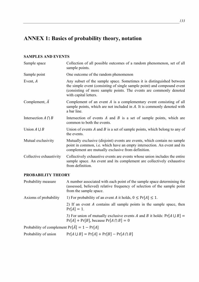
133
ANNEX 1: Basics of probability theory, notation
SAMPLES AND EVENTS
Sample space Collection of all possible outcomes of a random phenomenon, set of all
sample points.
Sample point One outcome of the random phenomenon
Event, Any subset of the sample space. Sometimes it is distinguished between
the simple event (consisting of single sample point) and compound event
(consisting of more sample points. The events are commonly denoted
with capital letters.
Complement, Complement of an event is a complementary event consisting of all
sample points, which are not included in . It is commonly denoted with
a bar line.
Intersection ⋂ Intersection of events and is a set of sample points, which are
common to both the events.
Union ⋃ Union of events and is a set of sample points, which belong to any of
the events.
Mutual exclusivity Mutually exclusive (disjoint) events are events, which contain no sample
point in common, i.e. which have an empty intersection. An event and its
complement are mutually exclusive from definition.
Collective exhaustivity Collectively exhaustive events are events whose union includes the entire
sample space. An event and its complement are collectively exhaustive
from definition.
PROBABILITY THEORY
Probability measure A number associated with each point of the sample space determining the
(assessed, believed) relative frequency of selection of the sample point
from the sample space.
Axioms of probability 1) For probability of an event it holds, [ ] .
2) If an event contains all sample points in the sample space, then
[ ] .
3) For union of mutually exclusive events and it holds: [ ⋃ ] [ ] [ ], because [ ⋂ ]
Probability of complement [ ] [ ]
Probability of union [ ⋃ ] [ ] [ ] [ ⋂ ]
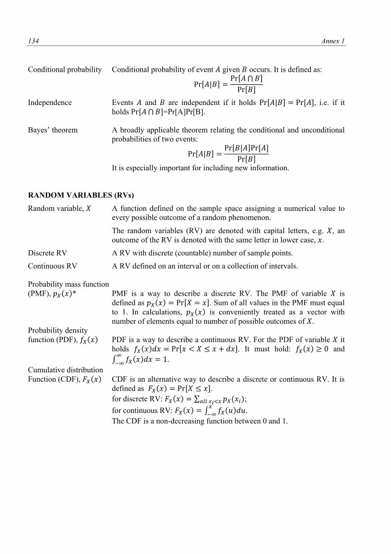
134 Annex 1
Conditional probability Conditional probability of event given occurs. It is defined as:
[ | ] [ ⋂ ]
[ ]
Independence Events and are independent if it holds [ | ] [ ], i.e. if it
holds [ ⋂ ]=Pr[A]Pr[B].
Bayes’ theorem A broadly applicable theorem relating the conditional and unconditional
probabilities of two events:
[ | ] [ | ] [ ]
[ ]
It is especially important for including new information.
RANDOM VARIABLES (RVs)
Random variable, A function defined on the sample space assigning a numerical value to
every possible outcome of a random phenomenon.
The random variables (RV) are denoted with capital letters, e.g. , an
outcome of the RV is denoted with the same letter in lower case, .
Discrete RV A RV with discrete (countable) number of sample points.
Continuous RV A RV defined on an interval or on a collection of intervals.
Probability mass function
(PMF), * PMF is a way to describe a discrete RV. The PMF of variable is
defined as [ ]. Sum of all values in the PMF must equal
to 1. In calculations, is conveniently treated as a vector with
number of elements equal to number of possible outcomes of .
Probability density
function (PDF), PDF is a way to describe a continuous RV. For the PDF of variable it
holds [ ]. It must hold: and
∫
.
Cumulative distribution
Function (CDF), CDF is an alternative way to describe a discrete or continuous RV. It is
defined as [ ].
for discrete RV: ∑ ;
for continuous RV: ∫
.
The CDF is a non-decreasing function between 0 and 1.
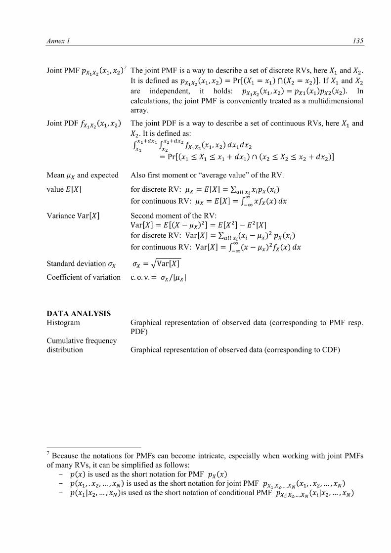
Annex 1 135
Joint PMF
7 The joint PMF is a way to describe a set of discrete RVs, here and .
It is defined as [ ⋂ ]. If and
are independent, it holds: In
calculations, the joint PMF is conveniently treated as a multidimensional
array.
Joint PDF The joint PDF is a way to describe a set of continuous RVs, here and
. It is defined as:
∫ ∫
[ ]
Mean and expected Also first moment or “average value” of the RV.
value [ ] for discrete RV: [ ] ∑
for continuous RV: [ ] ∫
Variance [ ] Second moment of the RV:
[ ] [ ] [ ] [ ]
for discrete RV: [ ] ∑
for continuous RV: [ ] ∫
Standard deviation √ [ ]
Coefficient of variation | |
DATA ANALYSIS
Histogram Graphical representation of observed data (corresponding to PMF resp.
PDF)
Cumulative frequency
distribution Graphical representation of observed data (corresponding to CDF)
7 Because the notations for PMFs can become intricate, especially when working with joint PMFs
of many RVs, it can be simplified as follows:
is used as the short notation for PMF is used as the short notation for joint PMF
| is used as the short notation of conditional PMF |
|

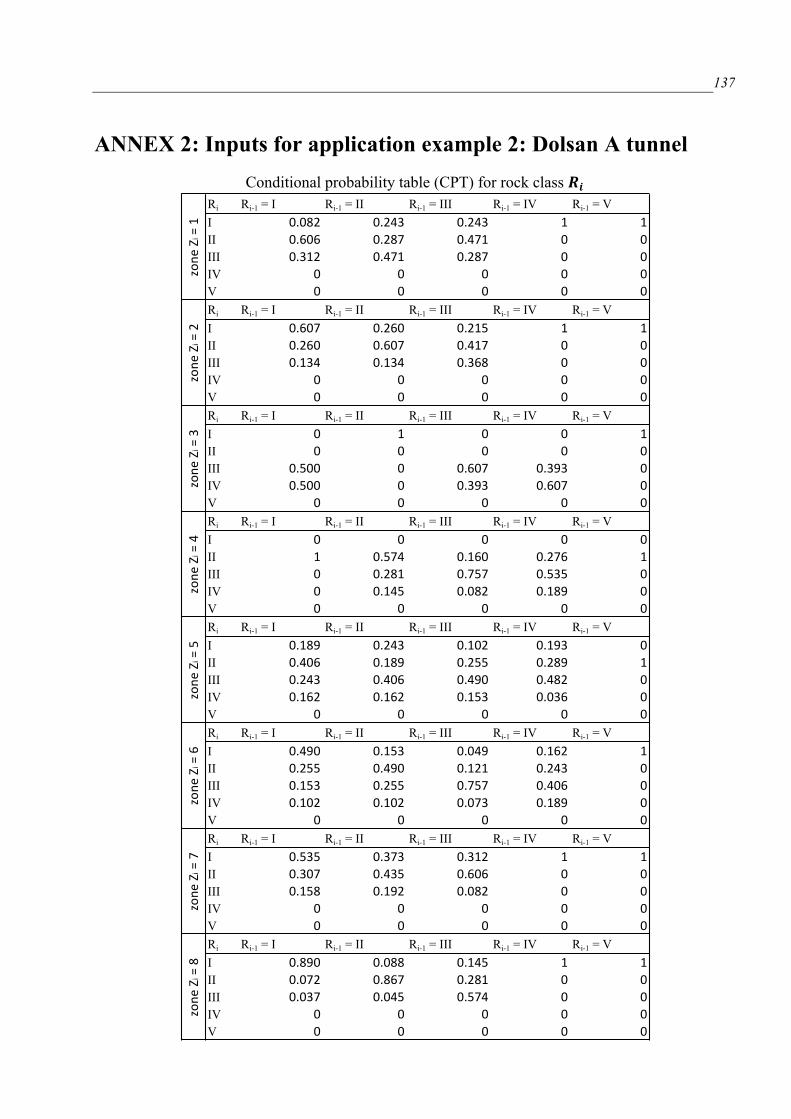
137
ANNEX 2: Inputs for application example 2: Dolsan A tunnel
Conditional probability table (CPT) for rock class
1 Annex2
Ri Ri-1 = I Ri-1 = II Ri-1 = III Ri-1 = IV Ri-1 = V
I 0.082 0.243 0.243 1 1
II 0.606 0.287 0.471 0 0
III 0.312 0.471 0.287 0 0
IV 0 0 0 0 0
V 0 0 0 0 0
Ri Ri-1 = I Ri-1 = II Ri-1 = III Ri-1 = IV Ri-1 = V
I 0.607 0.260 0.215 1 1
II 0.260 0.607 0.417 0 0
III 0.134 0.134 0.368 0 0
IV 0 0 0 0 0
V 0 0 0 0 0
Ri Ri-1 = I Ri-1 = II Ri-1 = III Ri-1 = IV Ri-1 = V
I 0 1 0 0 1
II 0 0 0 0 0
III 0.500 0 0.607 0.393 0
IV 0.500 0 0.393 0.607 0
V 0 0 0 0 0
Ri Ri-1 = I Ri-1 = II Ri-1 = III Ri-1 = IV Ri-1 = V
I 0 0 0 0 0
II 1 0.574 0.160 0.276 1
III 0 0.281 0.757 0.535 0
IV 0 0.145 0.082 0.189 0
V 0 0 0 0 0
Ri Ri-1 = I Ri-1 = II Ri-1 = III Ri-1 = IV Ri-1 = V
I 0.189 0.243 0.102 0.193 0
II 0.406 0.189 0.255 0.289 1
III 0.243 0.406 0.490 0.482 0
IV 0.162 0.162 0.153 0.036 0
V 0 0 0 0 0
Ri Ri-1 = I Ri-1 = II Ri-1 = III Ri-1 = IV Ri-1 = V
I 0.490 0.153 0.049 0.162 1
II 0.255 0.490 0.121 0.243 0
III 0.153 0.255 0.757 0.406 0
IV 0.102 0.102 0.073 0.189 0
V 0 0 0 0 0
Ri Ri-1 = I Ri-1 = II Ri-1 = III Ri-1 = IV Ri-1 = V
I 0.535 0.373 0.312 1 1
II 0.307 0.435 0.606 0 0
III 0.158 0.192 0.082 0 0
IV 0 0 0 0 0
V 0 0 0 0 0
Ri Ri-1 = I Ri-1 = II Ri-1 = III Ri-1 = IV Ri-1 = V
I 0.890 0.088 0.145 1 1
II 0.072 0.867 0.281 0 0
III 0.037 0.045 0.574 0 0
IV 0 0 0 0 0
V 0 0 0 0 0
zon
eZ
i=7
zon
eZ
i=8
ANNEX 2
Conditional probability table (CPT) for rock class Rizo
ne
Zi=
2zo
ne
Zi=
1zo
ne
Zi=
3zo
ne
Zi=
4zo
ne
Zi=
5zo
ne
Zi=
6
Input for application example 2: Dolsan A tunnel
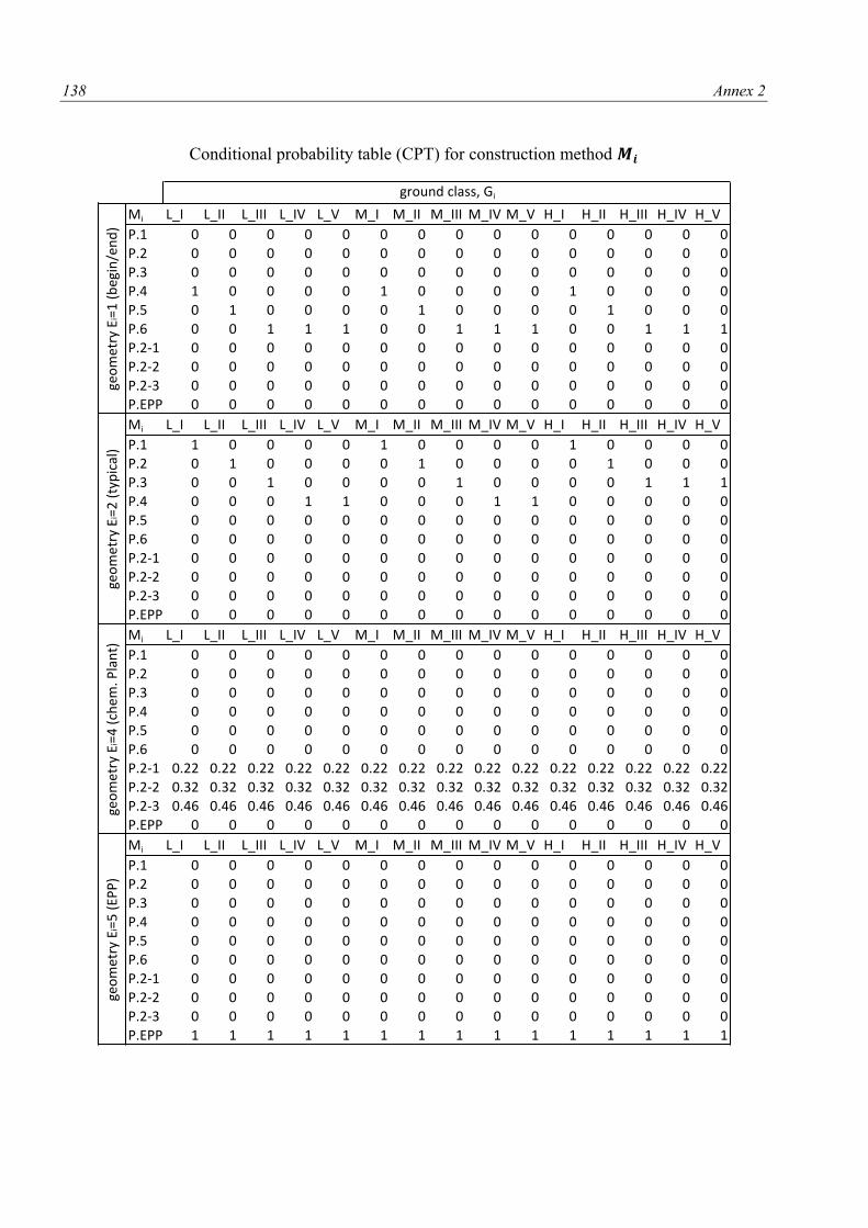
138 Annex 2
Conditional probability table (CPT) for construction method
3 Annex2
Mi L_I L_II L_III L_IV L_V M_I M_II M_III M_IV M_V H_I H_II H_III H_IV H_V
P.1 0 0 0 0 0 0 0 0 0 0 0 0 0 0 0
P.2 0 0 0 0 0 0 0 0 0 0 0 0 0 0 0
P.3 0 0 0 0 0 0 0 0 0 0 0 0 0 0 0
P.4 1 0 0 0 0 1 0 0 0 0 1 0 0 0 0
P.5 0 1 0 0 0 0 1 0 0 0 0 1 0 0 0
P.6 0 0 1 1 1 0 0 1 1 1 0 0 1 1 1
P.2-1 0 0 0 0 0 0 0 0 0 0 0 0 0 0 0
P.2-2 0 0 0 0 0 0 0 0 0 0 0 0 0 0 0
P.2-3 0 0 0 0 0 0 0 0 0 0 0 0 0 0 0
P.EPP 0 0 0 0 0 0 0 0 0 0 0 0 0 0 0
Mi L_I L_II L_III L_IV L_V M_I M_II M_III M_IV M_V H_I H_II H_III H_IV H_V
P.1 1 0 0 0 0 1 0 0 0 0 1 0 0 0 0
P.2 0 1 0 0 0 0 1 0 0 0 0 1 0 0 0
P.3 0 0 1 0 0 0 0 1 0 0 0 0 1 1 1
P.4 0 0 0 1 1 0 0 0 1 1 0 0 0 0 0
P.5 0 0 0 0 0 0 0 0 0 0 0 0 0 0 0
P.6 0 0 0 0 0 0 0 0 0 0 0 0 0 0 0
P.2-1 0 0 0 0 0 0 0 0 0 0 0 0 0 0 0
P.2-2 0 0 0 0 0 0 0 0 0 0 0 0 0 0 0
P.2-3 0 0 0 0 0 0 0 0 0 0 0 0 0 0 0
P.EPP 0 0 0 0 0 0 0 0 0 0 0 0 0 0 0
Mi L_I L_II L_III L_IV L_V M_I M_II M_III M_IV M_V H_I H_II H_III H_IV H_V
P.1 0 0 0 0 0 0 0 0 0 0 0 0 0 0 0
P.2 0 0 0 0 0 0 0 0 0 0 0 0 0 0 0
P.3 0 0 0 0 0 0 0 0 0 0 0 0 0 0 0
P.4 0 0 0 0 0 0 0 0 0 0 0 0 0 0 0
P.5 0 0 0 0 0 0 0 0 0 0 0 0 0 0 0
P.6 0 0 0 0 0 0 0 0 0 0 0 0 0 0 0
P.2-1 0.22 0.22 0.22 0.22 0.22 0.22 0.22 0.22 0.22 0.22 0.22 0.22 0.22 0.22 0.22
P.2-2 0.32 0.32 0.32 0.32 0.32 0.32 0.32 0.32 0.32 0.32 0.32 0.32 0.32 0.32 0.32
P.2-3 0.46 0.46 0.46 0.46 0.46 0.46 0.46 0.46 0.46 0.46 0.46 0.46 0.46 0.46 0.46
P.EPP 0 0 0 0 0 0 0 0 0 0 0 0 0 0 0
Mi L_I L_II L_III L_IV L_V M_I M_II M_III M_IV M_V H_I H_II H_III H_IV H_V
P.1 0 0 0 0 0 0 0 0 0 0 0 0 0 0 0
P.2 0 0 0 0 0 0 0 0 0 0 0 0 0 0 0
P.3 0 0 0 0 0 0 0 0 0 0 0 0 0 0 0
P.4 0 0 0 0 0 0 0 0 0 0 0 0 0 0 0
P.5 0 0 0 0 0 0 0 0 0 0 0 0 0 0 0
P.6 0 0 0 0 0 0 0 0 0 0 0 0 0 0 0
P.2-1 0 0 0 0 0 0 0 0 0 0 0 0 0 0 0
P.2-2 0 0 0 0 0 0 0 0 0 0 0 0 0 0 0
P.2-3 0 0 0 0 0 0 0 0 0 0 0 0 0 0 0
P.EPP 1 1 1 1 1 1 1 1 1 1 1 1 1 1 1
geo
met
ryE
i=5
(EP
P)
Conditional probability table (CPT) for construction method M i
groundclass,Gi
geo
met
ryE
i=1
(b
egin
/en
d)
geo
me
try
Ei=2
(ty
pic
al)
geo
me
try
Ei=
4(
chem
.Pla
nt)
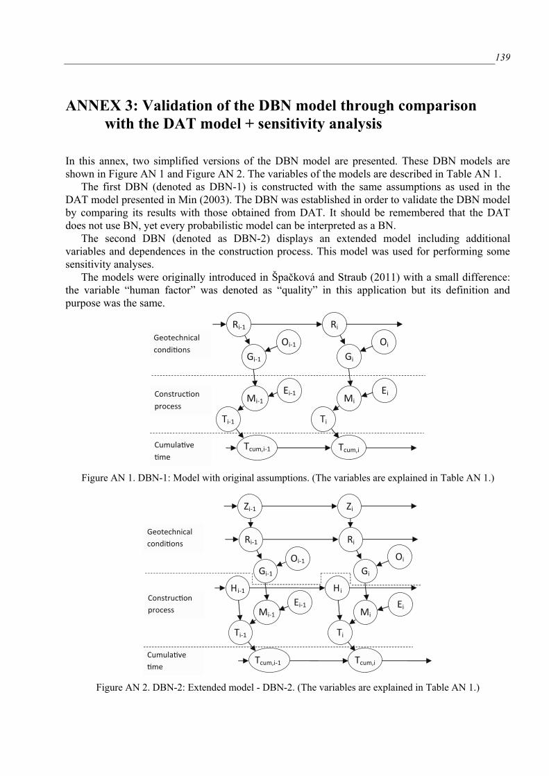
139
ANNEX 3: Validation of the DBN model through comparison
with the DAT model + sensitivity analysis
In this annex, two simplified versions of the DBN model are presented. These DBN models are
shown in Figure AN 1 and Figure AN 2. The variables of the models are described in Table AN 1.
The first DBN (denoted as DBN-1) is constructed with the same assumptions as used in the
DAT model presented in Min (2003). The DBN was established in order to validate the DBN model
by comparing its results with those obtained from DAT. It should be remembered that the DAT
does not use BN, yet every probabilistic model can be interpreted as a BN.
The second DBN (denoted as DBN-2) displays an extended model including additional
variables and dependences in the construction process. This model was used for performing some
sensitivity analyses.
The models were originally introduced in Špačková and Straub (2011) with a small difference:
the variable “human factor” was denoted as “quality” in this application but its definition and
purpose was the same.
Figure AN 1. DBN-1: Model with original assumptions. (The variables are explained in Table AN 1.)
Figure AN 2. DBN-2: Extended model - DBN-2. (The variables are explained in Table AN 1.)
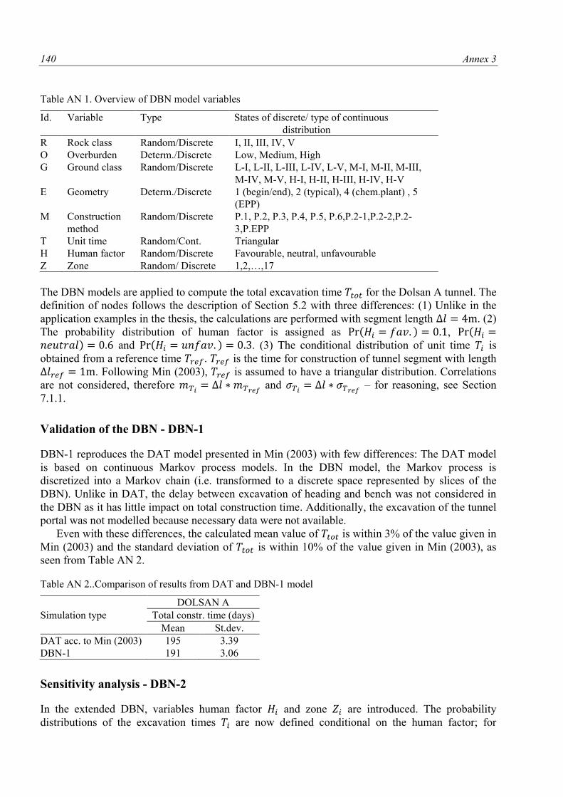
140 Annex 3
Table AN 1. Overview of DBN model variables
Id. Variable Type States of discrete/ type of continuous
distribution
R Rock class Random/Discrete I, II, III, IV, V
O Overburden Determ./Discrete Low, Medium, High
G Ground class Random/Discrete L-I, L-II, L-III, L-IV, L-V, M-I, M-II, M-III,
M-IV, M-V, H-I, H-II, H-III, H-IV, H-V
E Geometry Determ./Discrete 1 (begin/end), 2 (typical), 4 (chem.plant) , 5
(EPP)
M Construction
method
Random/Discrete P.1, P.2, P.3, P.4, P.5, P.6,P.2-1,P.2-2,P.2-
3,P.EPP
T Unit time Random/Cont. Triangular
H Human factor Random/Discrete Favourable, neutral, unfavourable
Z Zone Random/ Discrete 1,2,…,17
The DBN models are applied to compute the total excavation time for the Dolsan A tunnel. The
definition of nodes follows the description of Section 5.2 with three differences: (1) Unlike in the
application examples in the thesis, the calculations are performed with segment length . (2)
The probability distribution of human factor is assigned as , and . (3) The conditional distribution of unit time is
obtained from a reference time . is the time for construction of tunnel segment with length
. Following Min (2003), is assumed to have a triangular distribution. Correlations
are not considered, therefore
and
– for reasoning, see Section
7.1.1.
Validation of the DBN - DBN-1
DBN-1 reproduces the DAT model presented in Min (2003) with few differences: The DAT model
is based on continuous Markov process models. In the DBN model, the Markov process is
discretized into a Markov chain (i.e. transformed to a discrete space represented by slices of the
DBN). Unlike in DAT, the delay between excavation of heading and bench was not considered in
the DBN as it has little impact on total construction time. Additionally, the excavation of the tunnel
portal was not modelled because necessary data were not available.
Even with these differences, the calculated mean value of is within 3% of the value given in
Min (2003) and the standard deviation of is within 10% of the value given in Min (2003), as
seen from Table AN 2.
Table AN 2..Comparison of results from DAT and DBN-1 model
Simulation type
DOLSAN A
Total constr. time (days)
Mean St.dev.
DAT acc. to Min (2003) 195 3.39
DBN-1 191 3.06
Sensitivity analysis - DBN-2
In the extended DBN, variables human factor and zone are introduced. The probability
distributions of the excavation times are now defined conditional on the human factor; for
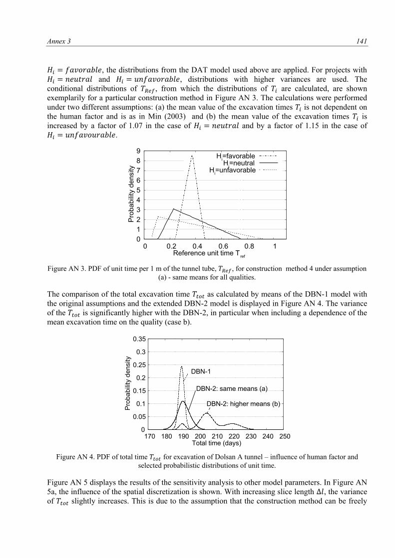
Annex 3 141
, the distributions from the DAT model used above are applied. For projects with
and , distributions with higher variances are used. The
conditional distributions of , from which the distributions of are calculated, are shown
exemplarily for a particular construction method in Figure AN 3. The calculations were performed
under two different assumptions: (a) the mean value of the excavation times is not dependent on
the human factor and is as in Min (2003) and (b) the mean value of the excavation times is
increased by a factor of 1.07 in the case of and by a factor of 1.15 in the case of
.
Figure AN 3. PDF of unit time per 1 m of the tunnel tube, , for construction method 4 under assumption
(a) - same means for all qualities.
The comparison of the total excavation time as calculated by means of the DBN-1 model with
the original assumptions and the extended DBN-2 model is displayed in Figure AN 4. The variance
of the is significantly higher with the DBN-2, in particular when including a dependence of the
mean excavation time on the quality (case b).
Figure AN 4. PDF of total time for excavation of Dolsan A tunnel – influence of human factor and
selected probabilistic distributions of unit time.
Figure AN 5 displays the results of the sensitivity analysis to other model parameters. In Figure AN
5a, the influence of the spatial discretization is shown. With increasing slice length , the variance
of slightly increases. This is due to the assumption that the construction method can be freely
0
1
2
3
4
5
6
7
8
9
0 0.2 0.4 0.6 0.8 1
Pro
ba
bili
ty d
ensity
Reference unit time Tref
Hi=favorableH
i=neutral
Hi=unfavorable
0
0.05
0.1
0.15
0.2
0.25
0.3
0.35
170 180 190 200 210 220 230 240 250
Pro
ba
bili
ty d
en
sity
Total time (days)
DBN-1
DBN-2: same means (a)
DBN-2: higher means (b)
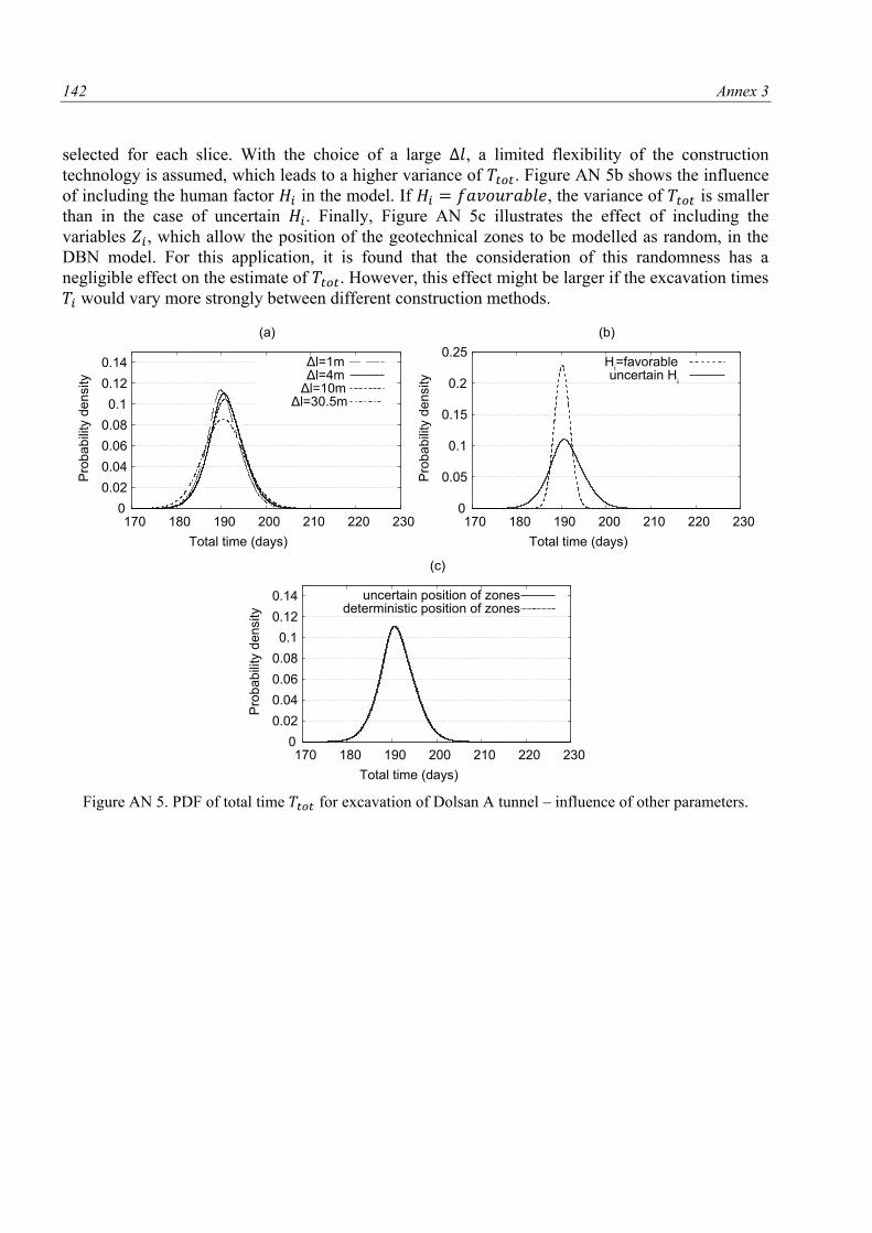
142 Annex 3
selected for each slice. With the choice of a large , a limited flexibility of the construction
technology is assumed, which leads to a higher variance of . Figure AN 5b shows the influence
of including the human factor in the model. If , the variance of is smaller
than in the case of uncertain . Finally, Figure AN 5c illustrates the effect of including the
variables , which allow the position of the geotechnical zones to be modelled as random, in the
DBN model. For this application, it is found that the consideration of this randomness has a
negligible effect on the estimate of . However, this effect might be larger if the excavation times
would vary more strongly between different construction methods.
Figure AN 5. PDF of total time for excavation of Dolsan A tunnel – influence of other parameters.
0
0.02
0.04
0.06
0.08
0.1
0.12
0.14
170 180 190 200 210 220 230
Pro
ba
bili
ty d
en
sity
Total time (days)
(a)
Δl=1mΔl=4mΔl=10m
Δl=30.5m
0
0.05
0.1
0.15
0.2
0.25
170 180 190 200 210 220 230
Pro
ba
bili
ty d
en
sity
Total time (days)
(b)
Hi=favorable
uncertain Hi
0
0.02
0.04
0.06
0.08
0.1
0.12
0.14
170 180 190 200 210 220 230
Pro
bab
ility
den
sity
Total time (days)
(c)
uncertain position of zonesdeterministic position of zones
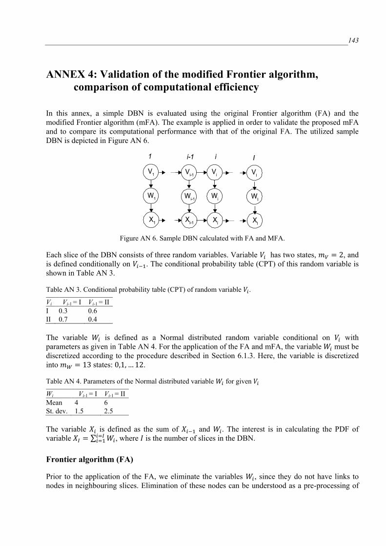
143
ANNEX 4: Validation of the modified Frontier algorithm,
comparison of computational efficiency
In this annex, a simple DBN is evaluated using the original Frontier algorithm (FA) and the
modified Frontier algorithm (mFA). The example is applied in order to validate the proposed mFA
and to compare its computational performance with that of the original FA. The utilized sample
DBN is depicted in Figure AN 6.
Figure AN 6. Sample DBN calculated with FA and MFA.
Each slice of the DBN consists of three random variables. Variable has two states, , and
is defined conditionally on . The conditional probability table (CPT) of this random variable is
shown in Table AN 3.
Table AN 3. Conditional probability table (CPT) of random variable .
Vi Vi-1 = I Vi-1 = II
I 0.3 0.6
II 0.7 0.4
The variable is defined as a Normal distributed random variable conditional on with
parameters as given in Table AN 4. For the application of the FA and mFA, the variable must be
discretized according to the procedure described in Section 6.1.3. Here, the variable is discretized
into states: .
Table AN 4. Parameters of the Normal distributed variable for given
Wi Vi-1 = I Vi-1 = II
Mean 4 6
St. dev. 1.5 2.5
The variable is defined as the sum of and . The interest is in calculating the PDF of
variable ∑ , where is the number of slices in the DBN.
Frontier algorithm (FA)
Prior to the application of the FA, we eliminate the variables , since they do not have links to
nodes in neighbouring slices. Elimination of these nodes can be understood as a pre-processing of
144 Annex 4
the DBN, reducing the computational demand during application of the FA. The elimination of
is performed for the whole DBN at once, variable is then defined directly on and on :
| ∑ | | , (1) .
where | is known from the discretization process of and
| | takes value 1 for and value 0
otherwise. The number of states of is .
One cycle of the FA, i.e. moving the Frontier from slice to slice , is shown in the
following. First, the variable is added and removed from the Frontier:
∑ | , (2) .
where | is defined in Table AN 5 and is the joint PMF known from previous
cycle of the FA.
Second, the variable is added and removed from the Frontier:
∑ | , (3) .
where | and are known from Eq. (1) and (2), respectively. Eq. (3)
represents the most demanding computational step in the algorithm. The computation of this
equation of the DBN requires time in the th slice. The evaluation the whole DBN
with slices therefore requires [ ] time. It is
evident that the computation time increases exponentially with the number of states of the variable
, , and with the number of slices of the DBN, .
Modified Frontier algorithm (mFA)
One cycle of the mFA is presented in the following. First, variable is added and is removed
from the Frontier according to Eq. (2). Second, the PMF of is calculated using convolution
(analogously to Eq. (6.19) and (6.20) from Section 6.2.3):
| |
| ∑ |
| , (4) .
where | | , | is known from the discretization of
variable and the summation is over all states of . Finally, the joint PMF describing the
Frontier in slice is calculated as | . The number of states of is increasing in each slice of the DBN; it is for
. The most demanding computational step of the mFA is the calculation of Eq. (4),
which in the th slice of the DBN requires time. For computation of the
convolution, the Fast Fourier Transform (FFT) is commonly used (Walker, 1996). With FFT, the
calculation of the th slice of the DBN requires time and evaluation of the
whole DBN with slices requires ∑ ∑ [
] time (Walker, 1996).
Annex 4 145
Analytical solution
Because the continuous variables in the DBN have conditional Normal distribution, the DBN can be
solved analytically by evaluating the moments of the variables. The evaluation proceeds slice by
slice, analogously with the previous algorithms. One cycle of the calculations is presented in the
following. The expected value and variance of the conditionally on is calculated as:
[ | ] [ | ] [ | ], (5) .
[ | ] [ | ] [ | ], (6) .
where [ | ] and [ | ] can be obtained from Table AN 6 and
[ | ] ∑ [ | ] [ | ] , (7) .
[ | ] ∑ [ | ] [ | ]
[ | ]. (8) .
[ | ] and [ | ] are known from the previous cycle of the calculation and the
conditional probability | | . The expected value and variance of the unconditional is calculated as:
[ ] ∑ [ ] [ | ] , (9) .
[ ] ∑ [ ] [ | ]
[ ], (10)
.
where
[ | ] [ | ] [ | ]. (11)
.
Eqs. (8) and (11) utilize an alternative calculation of variance using expression: [ ] [ ] [ ] - see Annex 1.
Results
Computations are performed for the DBN with varying number of slices . The computation times
depicted in Figure AN 7 show the theoretical computation time estimated based on the number of
performed operations as presented above and the observed time of computations performed in
Matlab on the computer specified in Section 6.3. The time needed for evaluation of the DBN with
only slices is almost 1000 times higher with the original FA than with the mFA. The
observed increase in computation time with the number of cycles is lower than the one estimated
above. The likely reason for this is that the FFT algorithm implemented in Matlab is more efficient
than the estimate given above (which represents a general upper bound).
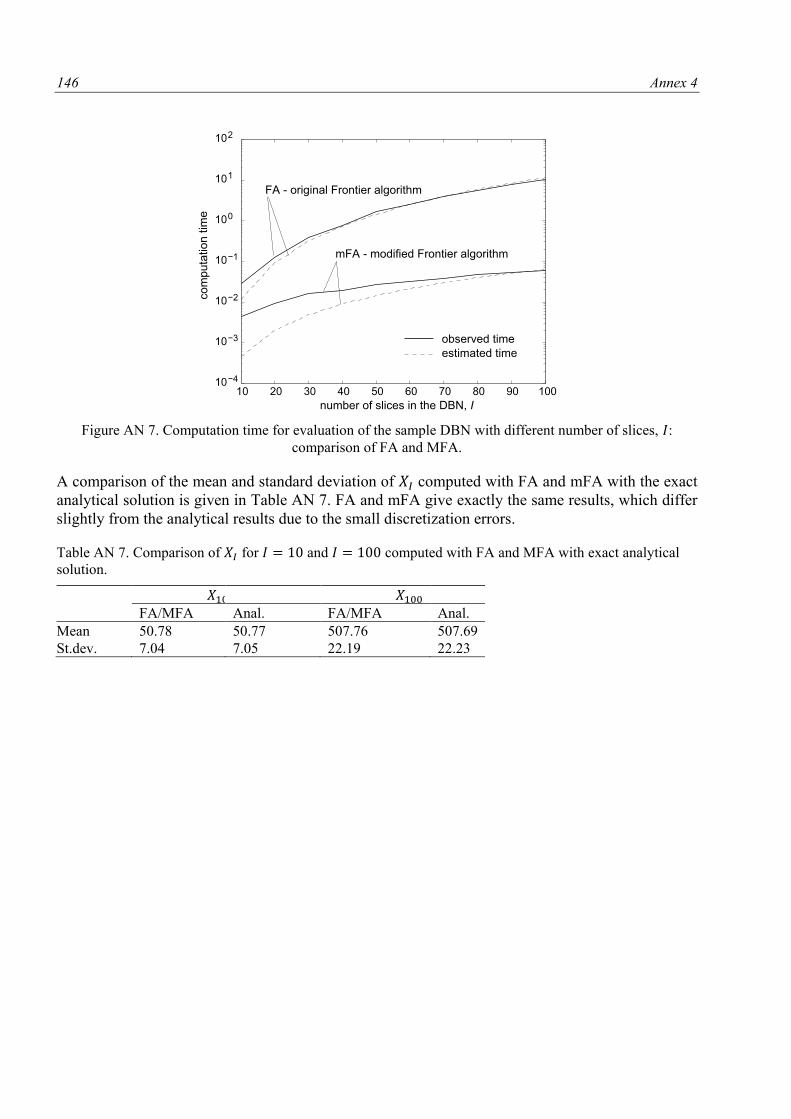
146 Annex 4
Figure AN 7. Computation time for evaluation of the sample DBN with different number of slices, : comparison of FA and MFA.
A comparison of the mean and standard deviation of computed with FA and mFA with the exact
analytical solution is given in Table AN 7. FA and mFA give exactly the same results, which differ
slightly from the analytical results due to the small discretization errors.
Table AN 7. Comparison of for and computed with FA and MFA with exact analytical
solution.
FA/MFA Anal. FA/MFA Anal.
Mean 50.78 50.77 507.76 507.69
St.dev. 7.04 7.05 22.19 22.23
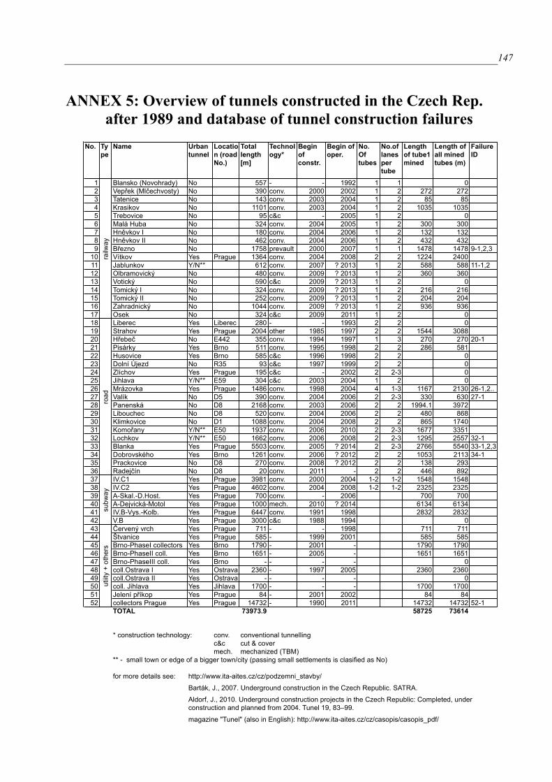
147
ANNEX 5: Overview of tunnels constructed in the Czech Rep.
after 1989 and database of tunnel construction failures
1 Annex 5
No. Ty
pe
Name Urban
tunnel
Locatio
n (road
No.)
Total
length
[m]
Technol
ogy*
Begin
of
constr.
Begin of
oper.
No.
Of
tubes
No.of
lanes
per
tube
Length
of tube1 -
mined
Length of
all mined
tubes (m)
Failure
ID
1 Blansko (Novohrady) No 557 - - 1992 1 1 0
2 Vepřek (Mlčechvosty) No 390 conv. 2000 2002 1 2 272 272
3 Tatenice No 143 conv. 2003 2004 1 2 85 85
4 Krasikov No 1101 conv. 2003 2004 1 2 1035 1035
5 Trebovice No 95 c&c - 2005 1 2 0
6 Malá Huba No 324 conv. 2004 2005 1 2 300 300
7 Hněvkov I No 180 conv. 2004 2006 1 2 132 132
8 Hněvkov II No 462 conv. 2004 2006 1 2 432 432
9 Březno No 1758 prevault 2000 2007 1 1 1478 1478 9-1,2,3
10 Vítkov Yes Prague 1364 conv. 2004 2008 2 2 1224 2400
11 Jablunkov Y/N** 612 conv. 2007 ? 2013 1 2 588 588 11-1,2
12 Olbramovický No 480 conv. 2009 ? 2013 1 2 360 360
13 Votický No 590 c&c 2009 ? 2013 1 2 0
14 Tomický I No 324 conv. 2009 ? 2013 1 2 216 216
15 Tomický II No 252 conv. 2009 ? 2013 1 2 204 204
16 Zahradnický No 1044 conv. 2009 ? 2013 1 2 936 936
17 Osek No 324 c&c 2009 2011 1 2 0
18 Liberec Yes Liberec 280 - - 1993 2 2 0
19 Strahov Yes Prague 2004 other 1985 1997 2 2 1544 3088
20 Hřebeč No E442 355 conv. 1994 1997 1 3 270 270 20-1
21 Pisárky Yes Brno 511 conv. 1995 1998 2 2 286 581
22 Husovice Yes Brno 585 c&c 1996 1998 2 2 0
23 Dolní Újezd No R35 93 c&c 1997 1999 2 2 0
24 Zlíchov Yes Prague 195 c&c - 2002 2 2-3 0
25 Jihlava Y/N** E59 304 c&c 2003 2004 1 2 0
26 Mrázovka Yes Prague 1486 conv. 1998 2004 4 1-3 1167 2130 26-1,2..
27 Valík No D5 390 conv. 2004 2006 2 2-3 330 630 27-1
28 Panenská No D8 2168 conv. 2003 2006 2 2 1994.1 3972
29 Libouchec No D8 520 conv. 2004 2006 2 2 480 868
30 Klimkovice No D1 1088 conv. 2004 2008 2 2 865 1740
31 Komořany Y/N** E50 1937 conv. 2006 2010 2 2-3 1677 3351
32 Lochkov Y/N** E50 1662 conv. 2006 2008 2 2-3 1295 2557 32-1
33 Blanka Yes Prague 5503 conv. 2005 ? 2014 2 2-3 2766 5540 33-1,2,3
34 Dobrovského Yes Brno 1261 conv. 2006 ? 2012 2 2 1053 2113 34-1
35 Prackovice No D8 270 conv. 2008 ? 2012 2 2 138 293
36 Radejčín No D8 20 conv. 2011 - 2 2 446 892
37 IV.C1 Yes Prague 3981 conv. 2000 2004 1-2 1-2 1548 1548
38 IV.C2 Yes Prague 4602 conv. 2004 2008 1-2 1-2 2325 2325
39 A-Skal.-D.Host. Yes Prague 700 conv. - 2006 700 700
40 A-Dejvická-Motol Yes Prague 1000 mech. 2010 ? 2014 6134 6134
41 IV.B-Vys.-Kolb. Yes Prague 6447 conv. 1991 1998 2832 2832
42 V.B Yes Prague 3000 c&c 1988 1994 0
43 Červený vrch Yes Prague 711 - - 1998 711 711
44 Štvanice Yes Prague 585 - 1999 2001 585 585
45 Brno-PhaseI collectors Yes Brno 1790 - 2001 - 1790 1790
46 Brno-PhaseII coll. Yes Brno 1651 - 2005 - 1651 1651
47 Brno-PhaseIII coll. Yes Brno - - - - 0
48 coll.Ostrava I Yes Ostrava 2360 - 1997 2005 2360 2360
49 coll.Ostrava II Yes Ostrava - - - - 0
50 coll. Jihlava Yes Jihlava 1700 - - - 1700 1700
51 Jelení příkop Yes Prague 84 - 2001 2002 84 84
52 collectors Prague Yes Prague 14732 - 1990 2011 14732 14732 52-1
TOTAL 73973.9 58725 73614
* construction technology: conv. conventional tunnelling
c&c cut & cover
mech. mechanized (TBM)
** - small town or edge of a bigger town/city (passing small settlements is clasified as No)
for more details see: http://www.ita-aites.cz/cz/podzemni_stavby/
Barták, J., 2007. Underground construction in the Czech Republic. SATRA.
magazine "Tunel" (also in English): http://www.ita-aites.cz/cz/casopis/casopis_pdf/
railw
ay
roa
dsu
bw
ay
utiity +
oth
ers
ANNEX 5 - Overview of tunnels constructed in the Czech Rep. after 1989 and database
of tunnel construction failures
Aldorf, J., 2010. Underground construction projects in the Czech Republic: Completed, under
construction and planned from 2004. Tunel 19, 83–99.
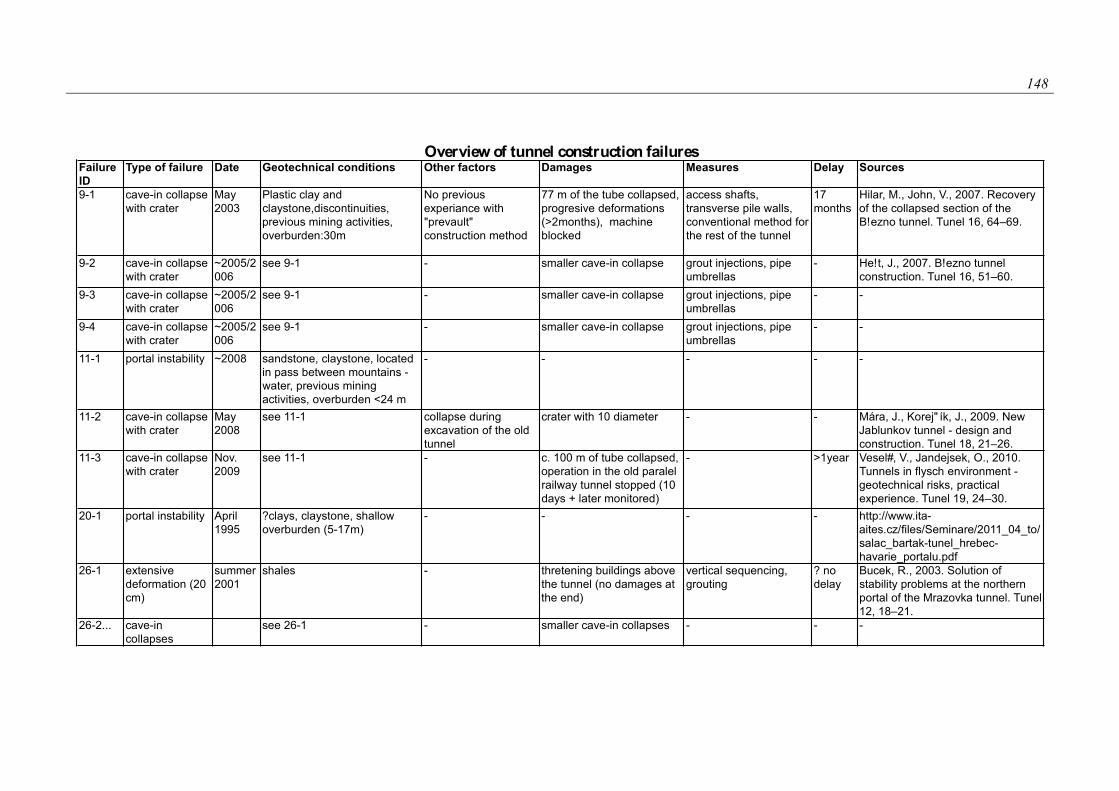
148
2 Annex 5
Failure
ID
Type of failure Date Geotechnical conditions Other factors Damages Measures Delay Sources
9-1 cave-in collapse
with crater
May
2003
Plastic clay and
claystone,discontinuities,
previous mining activities,
overburden:30m
No previous
experiance with
"prevault"
construction method
77 m of the tube collapsed,
progresive deformations
(>2months), machine
blocked
access shafts,
transverse pile walls,
conventional method for
the rest of the tunnel
17
months
Hilar, M., John, V., 2007. Recovery
of the collapsed section of the
B!ezno tunnel. Tunel 16, 64–69.
9-2 cave-in collapse
with crater
~2005/2
006
see 9-1 - smaller cave-in collapse grout injections, pipe
umbrellas
- He!t, J., 2007. B!ezno tunnel
construction. Tunel 16, 51–60.
9-3 cave-in collapse
with crater
~2005/2
006
see 9-1 - smaller cave-in collapse grout injections, pipe
umbrellas
- -
9-4 cave-in collapse
with crater
~2005/2
006
see 9-1 - smaller cave-in collapse grout injections, pipe
umbrellas
- -
11-1 portal instability ~2008 sandstone, claystone, located
in pass between mountains -
water, previous mining
activities, overburden <24 m
- - - - -
11-2 cave-in collapse
with crater
May
2008
see 11-1 collapse during
excavation of the old
tunnel
crater with 10 diameter - - Mára, J., Korej" ík, J., 2009. New
Jablunkov tunnel - design and
construction. Tunel 18, 21–26.
11-3 cave-in collapse
with crater
Nov.
2009
see 11-1 - c. 100 m of tube collapsed,
operation in the old paralel
railway tunnel stopped (10
days + later monitored)
- >1year Vesel#, V., Jandejsek, O., 2010.
Tunnels in flysch environment -
geotechnical risks, practical
experience. Tunel 19, 24–30.
20-1 portal instability April
1995
?clays, claystone, shallow
overburden (5-17m)
- - - - http://www.ita-
aites.cz/files/Seminare/2011_04_to/
salac_bartak-tunel_hrebec-
havarie_portalu.pdf
26-1 extensive
deformation (20
cm)
summer
2001
shales - thretening buildings above
the tunnel (no damages at
the end)
vertical sequencing,
grouting
? no
delay
Bucek, R., 2003. Solution of
stability problems at the northern
portal of the Mrazovka tunnel. Tunel
12, 18–21.
26-2... cave-in
collapses
see 26-1 - smaller cave-in collapses - - -
Overview of tunnel construction failures
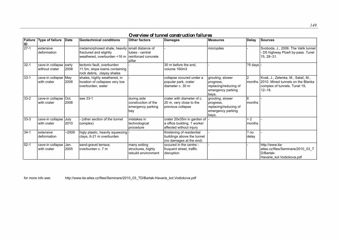
149
3 Annex 5
Failure
ID
Type of failure Date Geotechnical conditions Other factors Damages Measures Delay Sources
Overview of tunnel construction failures
27-1 extensive
deformation
metamorphosed shale, heavily
fractured and slightly
weathered, overburden <16 m
small distance of
tubes - central
reinforced concrete
pillar
- micropiles - Svoboda, J., 2006. The Valík tunnel
- D5 highway Plzeň by-pass. Tunel
15, 28–31.
32-1 cave-in collapse
without crater
early
2008
tectonic fault, overburden
11.5m, slope loams containing
rock debris, clayey shales
- 30 m before the end,
volume 160m3
- ?5 days -
33-1 cave-in collapse
with crater
May
2008
shales, highly weathered, in
location of collapses very low
overburden, water
- collapse occured under a
popular park, crater
diameter c. 30 m
grouting, slower
progress,
replacing/reducing of
emergency parking
bays,
2
months
Kvaš, J., Zelenka, M., Salač, M.,
2010. Mined tunnels on the Blanka
complex of tunnels. Tunel 19,
12–18.
33-2 cave-in collapse
with crater
Oct.
2008
see 33-1 during side
construciton of the
emergency parking
bay
crater with diameter of c.
20 m, very close to the
previous collapse
grouting, slower
progress,
replacing/reducing of
emergency parking
bays,
6
months
-
33-3 cave-in collapse
with crater
July
2010
- (other section of the tunnel
complex)
mistakes in
technological
procedure
crater 20x35m in garden of
a office building, 1 worker
affected without injury
- > 2
months
-
34-1 extensive
deformation
~2009 higly plastic, heavily squeezing
clays, 6-21 m overburden
- thretening of residential
buildings above the tunnel
(no damages at the end)
- ? no
delay
-
52-1 cave-in collapse
with crater
Jan.
2005
sand-gravel terrace,
overburden c. 7 m
many exiting
structures, highly
rebuild environment
occured in the centre -
fruquent street, traffic
disruption
- - http://www.ita-
aites.cz/files/Seminare/2010_03_T
D/Bartak-
Havarie_kol.Vodickova.pdf
for more info see: http://www.ita-aites.cz/files/Seminare/2010_03_TD/Bartak-Havarie_kol.Vodickova.pdf

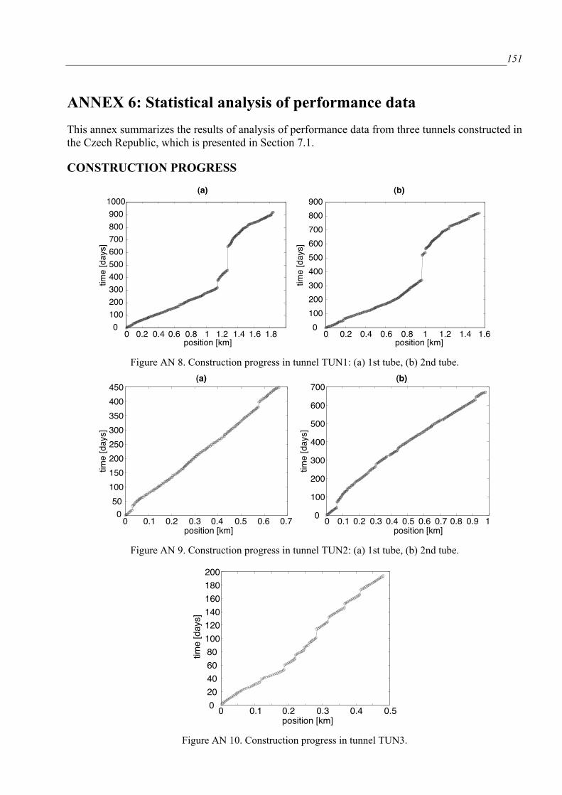
151
ANNEX 6: Statistical analysis of performance data
This annex summarizes the results of analysis of performance data from three tunnels constructed in
the Czech Republic, which is presented in Section 7.1.
CONSTRUCTION PROGRESS
Figure AN 8. Construction progress in tunnel TUN1: (a) 1st tube, (b) 2nd tube.
Figure AN 9. Construction progress in tunnel TUN2: (a) 1st tube, (b) 2nd tube.
Figure AN 10. Construction progress in tunnel TUN3.
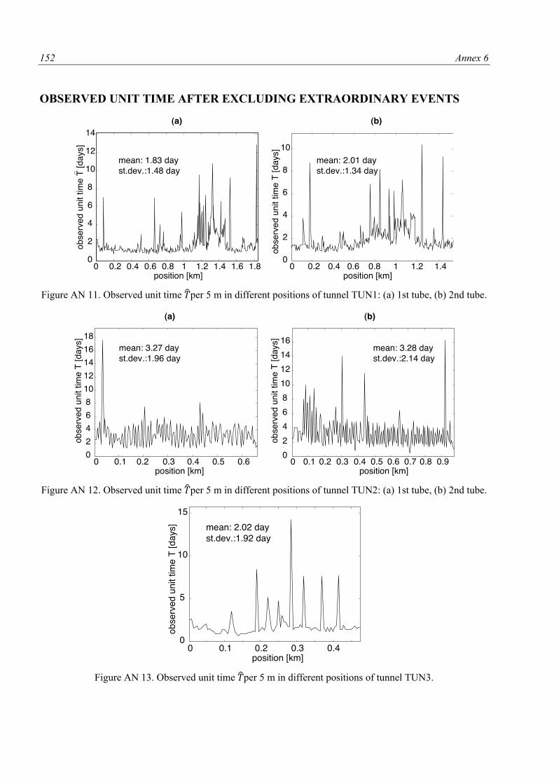
152 Annex 6
OBSERVED UNIT TIME AFTER EXCLUDING EXTRAORDINARY EVENTS
Figure AN 11. Observed unit time per 5 m in different positions of tunnel TUN1: (a) 1st tube, (b) 2nd tube.
Figure AN 12. Observed unit time per 5 m in different positions of tunnel TUN2: (a) 1st tube, (b) 2nd tube.
Figure AN 13. Observed unit time per 5 m in different positions of tunnel TUN3.
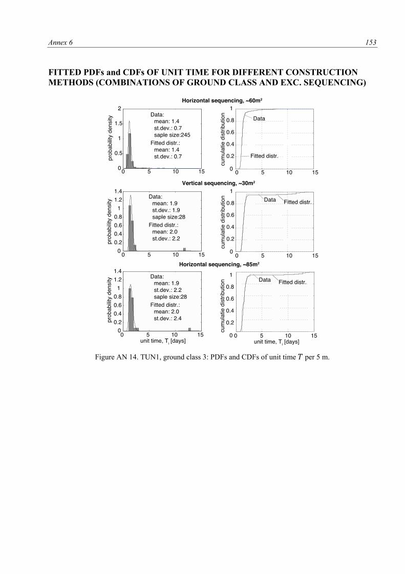
Annex 6 153
FITTED PDFs and CDFs OF UNIT TIME FOR DIFFERENT CONSTRUCTION
METHODS (COMBINATIONS OF GROUND CLASS AND EXC. SEQUENCING)
Figure AN 14. TUN1, ground class 3: PDFs and CDFs of unit time per 5 m.
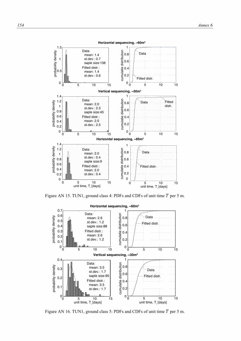
154 Annex 6
Figure AN 15. TUN1, ground class 4: PDFs and CDFs of unit time per 5 m.
Figure AN 16. TUN1, ground class 5: PDFs and CDFs of unit time per 5 m.
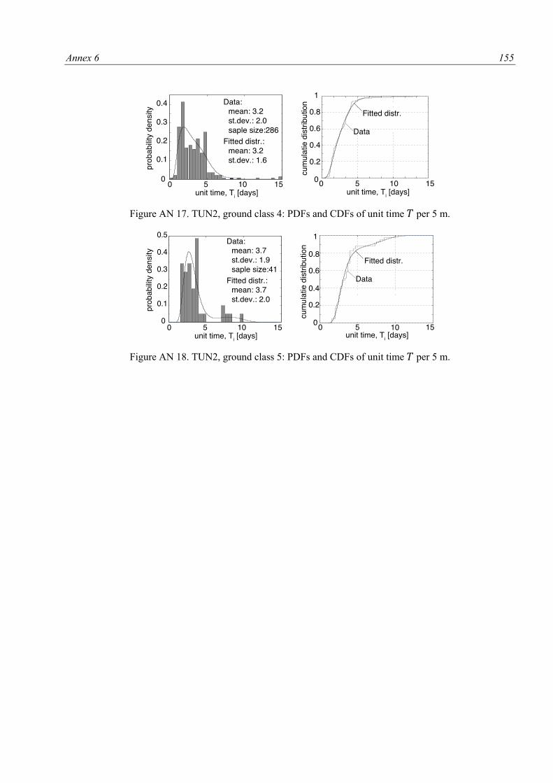
Annex 6 155
Figure AN 17. TUN2, ground class 4: PDFs and CDFs of unit time per 5 m.
Figure AN 18. TUN2, ground class 5: PDFs and CDFs of unit time per 5 m.
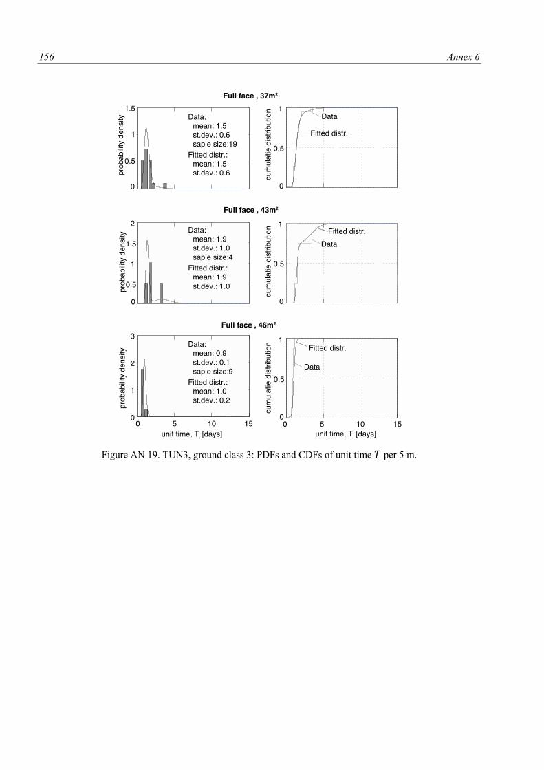
156 Annex 6
Figure AN 19. TUN3, ground class 3: PDFs and CDFs of unit time per 5 m.
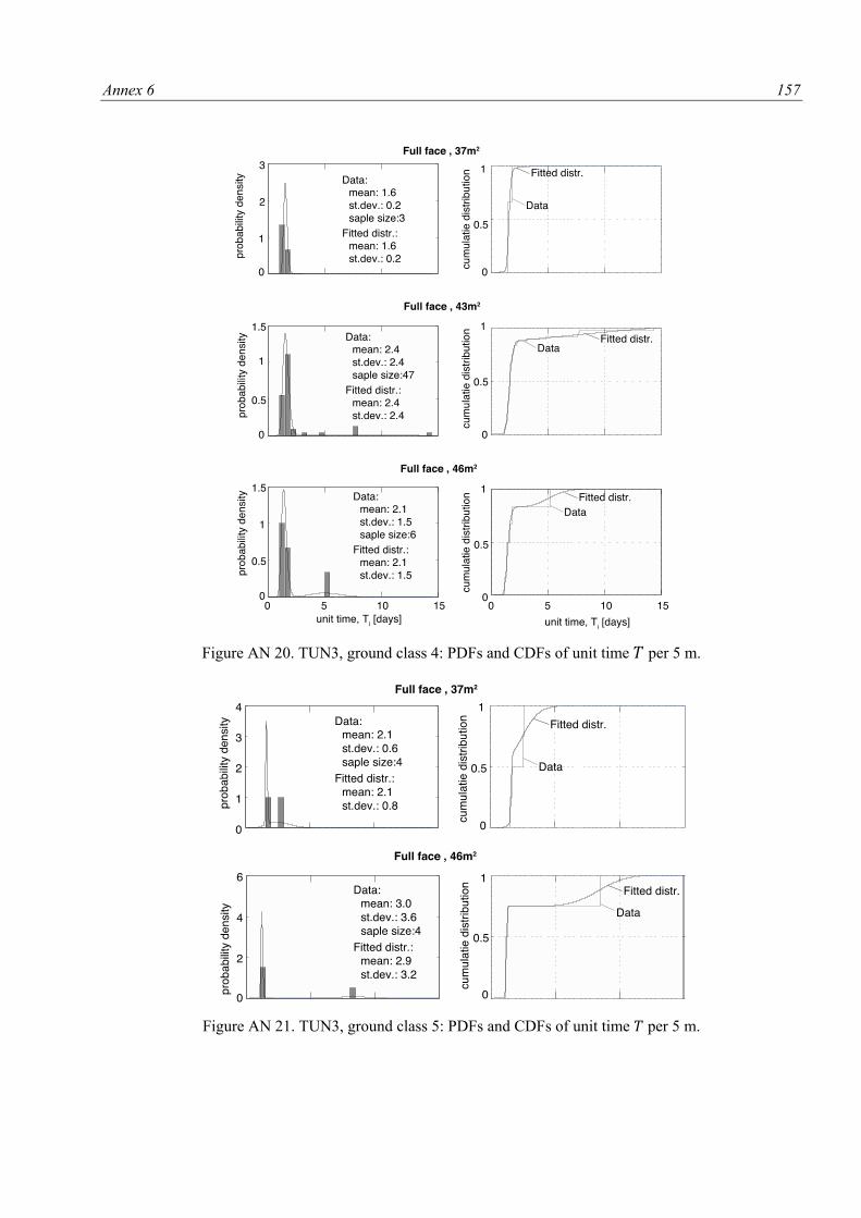
Annex 6 157
Figure AN 20. TUN3, ground class 4: PDFs and CDFs of unit time per 5 m.
Figure AN 21. TUN3, ground class 5: PDFs and CDFs of unit time per 5 m.

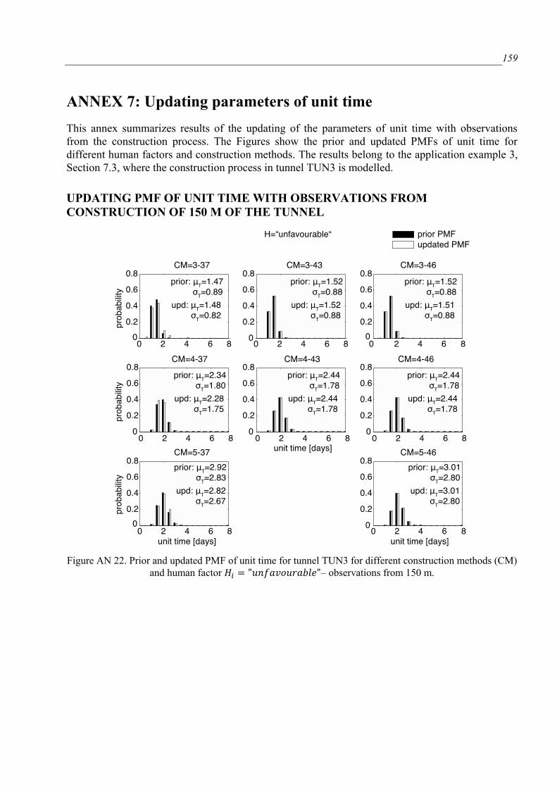
159
ANNEX 7: Updating parameters of unit time
This annex summarizes results of the updating of the parameters of unit time with observations
from the construction process. The Figures show the prior and updated PMFs of unit time for
different human factors and construction methods. The results belong to the application example 3,
Section 7.3, where the construction process in tunnel TUN3 is modelled.
UPDATING PMF OF UNIT TIME WITH OBSERVATIONS FROM
CONSTRUCTION OF 150 M OF THE TUNNEL
Figure AN 22. Prior and updated PMF of unit time for tunnel TUN3 for different construction methods (CM)
and human factor – observations from 150 m.
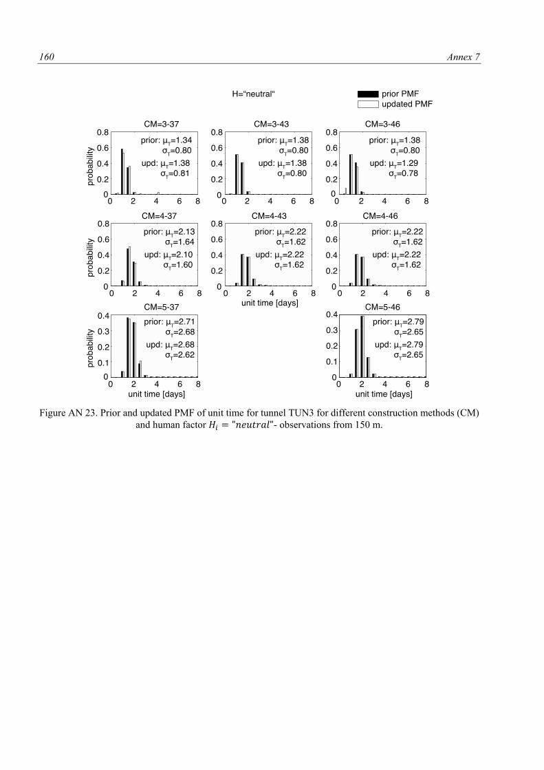
160 Annex 7
Figure AN 23. Prior and updated PMF of unit time for tunnel TUN3 for different construction methods (CM)
and human factor - observations from 150 m.
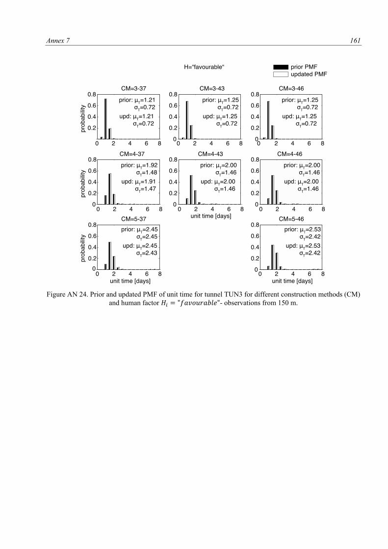
Annex 7 161
Figure AN 24. Prior and updated PMF of unit time for tunnel TUN3 for different construction methods (CM)
and human factor - observations from 150 m.
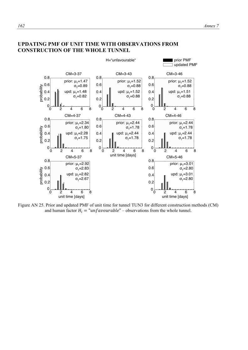
162 Annex 7
UPDATING PMF OF UNIT TIME WITH OBSERVATIONS FROM
CONSTRUCTION OF THE WHOLE TUNNEL
Figure AN 25. Prior and updated PMF of unit time for tunnel TUN3 for different construction methods (CM)
and human factor – observations from the whole tunnel.
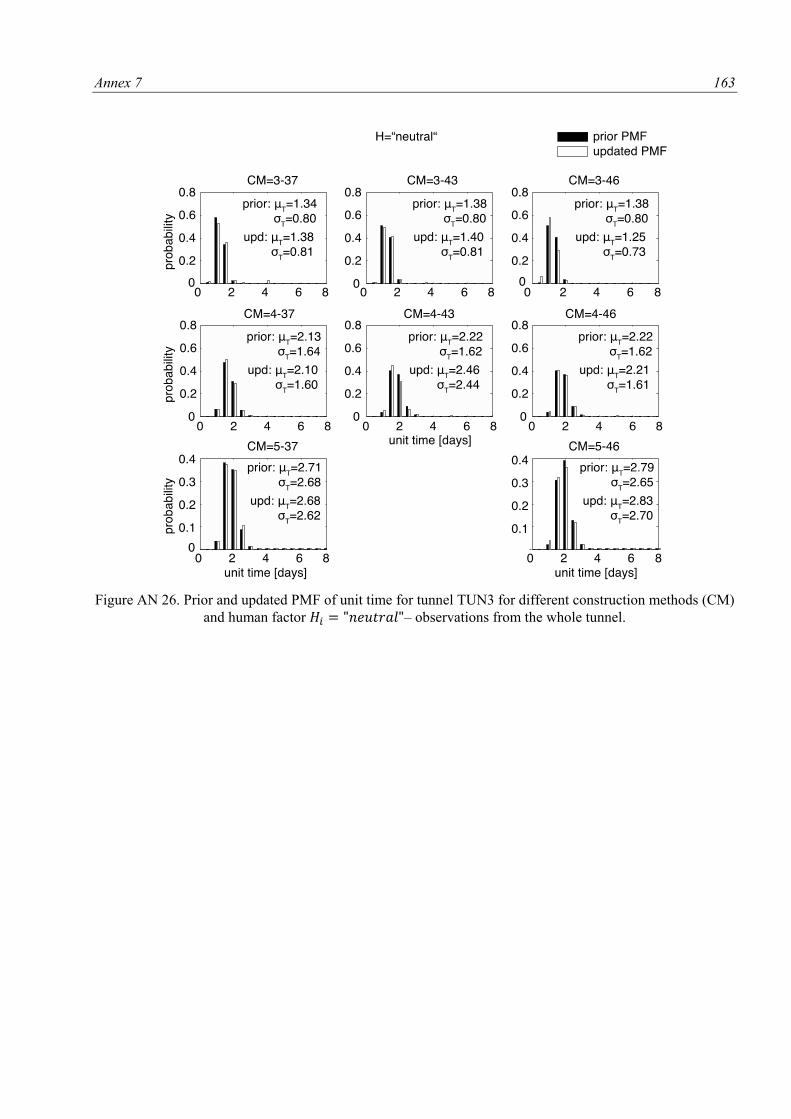
Annex 7 163
Figure AN 26. Prior and updated PMF of unit time for tunnel TUN3 for different construction methods (CM)
and human factor – observations from the whole tunnel.
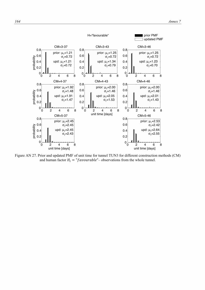
164 Annex 7
Figure AN 27. Prior and updated PMF of unit time for tunnel TUN3 for different construction methods (CM)
and human factor – observations from the whole tunnel.