CHAPTER SIX

CW-EPR Spectral Simulations:Solid State☆

Stefan Stoll1Department of Chemistry, University of Washington, Seattle, Washington, USA1Corresponding author: e-mail address: stst@uw.edu

Contents

1. Introduction 1222. Spins and SH 1233. Dynamic Regime 1274. Levels of Theory 128

4.1 Calculation of Energy Levels 1284.2 Energy Level Diagram Modeling 1294.3 Eigenfields 130

5. Orientational Order and Disorder 1315.1 Crystals 1315.2 Powders 1325.3 Partially Ordered Samples 133

6. Structural Order and Disorder 1347. Other Line Broadenings 1358. Experimental Effects 136

8.1 Field Modulation 1368.2 Saturation 1378.3 RC Filtering 137

9. Fitting 1379.1 Objective Function 1389.2 Parameter Starting Point and Search Range 1389.3 Fitting Algorithm 139

10. Conclusions 139References 140

Abstract

This chapter summarizes the core concepts underlying the simulation of EPR spectrafrom biological samples in the solid state, from a user perspective. The key choicesand decisions that have to be made by a user when simulating an experimental EPR

☆This chapter is dedicated to Graeme Hanson (1955–2015), the creator of the EPR simulation program

XSophe.

Methods in Enzymology, Volume 563 # 2015 Elsevier Inc.ISSN 0076-6879 All rights reserved.http://dx.doi.org/10.1016/bs.mie.2015.06.003

121

spectrum are outlined. These include: the choice of the simulation model (the networkof spins and the associated spin Hamiltonian), the dynamic regime (solid, liquid, slowmotion), the level of theory used in the simulation (matrix diagonalization, perturbationtheory, etc.), the treatment of orientational order and disorder (powder, crystal, partialordering), the inclusion of the effects of structural disorder (strains), the effects of otherline broadening mechanisms (unresolved hyperfine couplings, relaxation), and theinclusion of experimental distortions (field modulation, power saturation, filtering).Additionally, the salient aspects of utilizing least-squares fitting algorithms to aid theanalysis of experimental spectra with the help of simulations are outlined. Althoughdrawing from the experience gained from implementing EasySpin and from interactingwith EasySpin's user base, this chapter applies to any EPR simulation software.

1. INTRODUCTION

In enzymology, biochemistry, and structural biophysics, solid-state

EPR spectroscopy is used in two main contexts. First, it is used to study

the structures of resting and intermediate states of radical enzymes,

metalloenzymes, and metalloproteins which are constitutively paramagnetic

(transition metal ions; metal ion clusters; protein-, substrate-, and cofactor-

centered organic radicals). Second, solid-state EPR is used to determine

conformations of proteins and protein complexes that are intrinsically dia-

magnetic, but are rendered paramagnetic by the site-selective introduction

of spin labels.

The structure of the paramagnetic centers in these systems can be very

rich and varied. As a consequence, they can give rise to a wide range of very

diverse EPR spectra that often can only be analyzed with the help of com-

puter simulations. Therefore, in addition to being familiar with published

EPR spectra of the type of centers under study, a practitioner of EPR needs

to be aware of the choices required in an EPR simulation. Improper choices

can lead to erroneous conclusions, even if the simulations appear to be accu-

rate and are perceived as correct.

In this overview, we review the concepts underlying the essential deci-

sions that need to be taken when simulating and fitting EPR spectra. This

provides a framework for performing robust EPR simulations, while min-

imizing the risk of making wrong conclusions from the data. This frame-

work is general and independent of any particular simulation program.

The author’s program, EasySpin (Stoll & Schweiger, 2006), offers many

choices on all aspects, whereas many other programs are more limited in

scope (although just as correct within their scope, and often faster). The

aspects discussed in this chapter are based on the experience gained from

122 Stefan Stoll

implementing EasySpin and from interacting with its user base over the

years, but are valid more generally.

This chapter will not discuss the theory underlying EPR simulations. For

more details about that, see a recent comprehensive review on the subject

(Stoll, 2014) that includes over 500 references. The general theory of solid-

state EPR is laid out in several excellent textbooks and monographs

(Abragam & Bleaney, 1986; Atherton, 1993; Bencini & Gatteschi, 1990;

Mabbs & Collison, 1992; Pake & Estle, 1973; Pilbrow, 1990; Weil &

Bolton, 2007).

The basic workflow for setting up an EPR simulation is as follows. First,

an appropriate spin coupling network and an appropriate spin Hamiltonian

(SH) model have to be chosen (Section 2). This is trivial for systems such as

nitroxide radicals or copper complexes, but can be challenging if the molec-

ular species giving rise to the EPR signal is not established. Second, the

dynamical regime must be identified. This can be liquid, slow-motion, or

rigid limit and depends on the rotational mobility of the paramagnetic center

and potentially other dynamical processes. In this overview, we only discuss

solid-state samples in the rigid-limit regime (Section 3). Third, an adequate

and sufficiently accurate level of theory suitable to calculate EPR spectra

from the given SH needs to be selected (Section 4). Most commonly, this

is either matrix diagonalization or perturbation theory in combination with

some sort of energy level diagram modeling. Fourth, knowledge of the ori-

entational order or disorder of the sample is required (Section 5). This can be

a powder, a crystal of a specific symmetry, or a partially ordered phase. Fifth,

a decision has to be made as to how to model additional broadenings

resulting from structural disorder, magnetic disorder, and relaxation pro-

cesses (Sections 6 and 7). Sixth, it has to be ascertained that experimental

effects due to saturation, field modulation, and filtering are properly

accounted for (Section 8). Lastly, if the purpose of the simulation is to fit

experimental data, then considerations about the type, scope, and utility

of various least-squares fitting algorithms are important (Section 9).

2. SPINS AND SH

Most molecular paramagnetic systems can be simulated using a SH,

which is an effective Hamiltonian that only depends on the spins of electrons

and magnetic nuclei, and not their spatial coordinates. Effects of the crystal

field and of spin–orbit coupling are folded into the parameters of this SH

(Weil & Bolton, 2007).

123Solid-State CW-EPR Simulations

The first decision to be made when setting up an EPR simulation is the

number and types of electron and nuclear spins to include. Often, this is very

obvious, especially for the electron spins. For example, for an organic rad-

ical, an electron spin of S¼1/2 is evident. On a single transition metal ion,

all unpaired electrons are treated as a single total spin S. For example, for

high-spin Fe(III) with five unpaired electrons, it would be S¼5/2. How-

ever, for multiple coupled paramagnets, this can be less obvious. In a cluster

of metal ions, there are two possibilities. First, one can treat the spins on each

ion explicitly and then include appropriate coupling terms into the SH. Sec-

ond, if the coupling is sufficiently strong and only the lowest energy levels

are observable by EPR, the entire metal ion cluster can be treated as a single

total electron spin Stot. For example, an antiferromagnetically coupled

Fe(II)Fe(III) cluster can be modeled as a system with a Fe(II) with S1¼2

coupled to an Fe(III) with S2¼5/2, or as a single total spin with Stot¼1/2.

The choice between these uncoupled and coupled representations depends

on the available experimental data and on the level of analysis that is desired

(Bencini & Gatteschi, 1990).

The inclusion of nuclear spins also needs consideration. In a Cu(II) com-

plex, one obviously must include the Cu nuclear spin. Sometimes, it is also

necessary to include magnetic nuclei from the ligands. The decision of

whether to include a magnetic nucleus explicitly in the SH depends on

whether the effects from its hyperfine coupling to the electron spins are

resolved or not. If they are resolved, the nucleus must be modeled explicitly.

If they are not resolved, but only result in additional broadening, they should

be treated as a line broadening mechanism (see Section 7).

Once the network of spins is chosen, the SH terms describing the inter-

actions of the spins need to be chosen. SHs that allow accurate simulation of

the EPR spectra from the great majority of paramagnetic systems contain

only a few types of terms. These are listed in the following.

(A) ElectronZeeman interaction. For each electron spin in the system, a term

of the form HEZI ¼ μBBgS must be included, with the Bohr magneton

μB (in J/T), the magnetic field vector B (in T), and the spin vector oper-

ator S (unitless). The 3�3matrix, g, is called the g tensor or gmatrix. For

a free electron outside a molecular environment, it is diagonal and iso-

tropic, with ge¼ 2:002319 on the diagonal. In the presence of a molec-

ular electrostatic environment it shifts from ge. This g shift,Δg¼ g� ge, is

generally anisotropic in the sense that it depends on the orientation of the

molecule with respect to the applied magnetic field. The g shift can be

124 Stefan Stoll

interpreted in terms of molecular structural and electronic properties

(Patchkovskii & Schreckenbach, 2004; Stoll, 2011).

(B) For each electron spin with spin >1/2, a zero-field splitting term is

included in the SH. Its form is HZFI¼ SDS, with the 3�3 matrix

D representing the zero-field interaction tensor, in energy units.

The origin of these terms lies in the spin–spin interactions of the elec-

trons constituting the spin >1/2, and in spin–orbit coupling (Neese,

2004). The zero-field interaction is often parameterized in terms of

the scalar parameters D and E (Weil & Bolton, 2007). Typical values

of D range from around 0.1 cm�1 for organic triplet radicals to

10 cm�1 and larger for high-spin transition metal centers.

(C) For electron spins with spin 3/2 and larger (e.g., in high-spin transition

metal ions), it can be necessary to include higher-order zero-field terms

proportional to S4 and S6 in the SH. There is a wide and confusing

range of different conventions used for these terms (Rudowicz &

Karbowiak, 2015). The predominant approach involves a linear com-

bination of extended Stevens operators. For systems with cubic sym-

metry, the more traditional scalar parameters a and F are often

employed instead (Abragam & Bleaney, 1986). The structural origin

of these terms is usually the crystal field.

(D) For each pair of interacting electron spins, a coupling term has to be

included in the SH. The most general form of this coupling is

Hee¼ SAJ SB, with the 3�3 interaction matrix J, in energy units.

The interaction can be broken down into three terms (Bencini &

Gatteschi, 1990): (a) an isotropic term J0SASB, often called the

Heisenberg–Dirac–van Vleck (HDvV) Hamiltonian, with the isotro-

pic exchange coupling constant J0 (note that different conventions

are used in the literature); (b) an antisymmetric exchange term written

as dABSA� SB with the parameter vector dAB and called the

Dzyaloshinskii–Moriya term; and (c) a dipolar term SADABSB with

the traceless 3�3 matrix DAB describing dipolar interactions. Very

often, the isotropic component dominates, and the other two terms

are neglected.

(E) Beyond these standard SH terms for the electron spins, there are others

withmuch rarer occurrence. These terms include biquadratic exchange

�j SASB� �2

(Harris & Owen, 1963) and high-order Zeeman terms of

dimension BS3 and BS5 (Claridge, Tennant, & McGavin, 1997). Very

125Solid-State CW-EPR Simulations

few simulation programs implement them explicitly (Mombourquette,

Tennant, & Weil, 1986).

(F) For each pair of nuclear spin and electron spin, a hyperfine coupling

term is included in the SH. Its form is HHFI¼ SAI, with the 3�3

hyperfine matrix A, in energy units, and the nuclear spin vector oper-

ator I (unitless). The hyperfine interaction can be decomposed into

three terms of different physical origin: (a) the isotropic Fermi contact

term A0SI, (b) the through-space spin-dipolar coupling term SAdipI

with the traceless matrix Adip, and (c) the spin–orbit term SAorbI with

the 3�3 coupling matrix Aorb. This last term can be neglected in

organic radicals, but must be taken into account in transition metals

with large spin–orbit coupling (i.e., large g shifts).

(G) For each nuclear spin that is included in the SH model, there is a

nuclear Zeeman term of the form HNZI¼�μNgnBI, with the nuclear

magneton μN (in J/T) and the nuclear g factor gn (unitless), which is an

isotope-specific constant that ranges from about �4 to +6. In molec-

ular environments, gn is slightly shifted from its free atom value and is

anisotropic. This chemical shift anisotropy is in the ppm range and

is too small to be resolved in EPR experiments. Therefore, it is always

neglected and omitted from the SH.

(H) Finally, for each nuclear spin with spin>1/2, a nuclear quadrupole term

of the form HNQI¼ IQI is present in the SH.Q is the 3�3 matrix that

describes the interaction of the nuclear electric quadrupole moment

with the local electric field gradient. Effects of this term can occasionally

be observed in CW-EPR spectra of 5d transition metals ions (Shaw

et al., 2006). For CW-EPR of biologically abundant first-row transition

metal ions and for organic radicals, this term can be generally neglected.

In these cases, pulse EPR can be used to resolve this term.

(I) Lastly, there exists nuclear spin–spin coupling between each pair of

magnetic nuclei in a molecule, both through-space and through-bond.

Since the energies of these interactions are very low, they are not resolv-

able by EPR and are neglected in EPR simulations.

The SH terms listed above rely on the assumption that the electronic ground

state observed by EPR is orbitally nondegenerate and that spin–orbit cou-

pling is weak enough that it can be treated using second-order perturbation

theory.When the ground state is orbitally degenerate, or the spin–orbit cou-

pling is substantial, the explicit inclusion of orbital angular momentum

effects is necessary. This can be achieved by going beyond the SH

126 Stefan Stoll

approximation and introducing into the Hamiltonian terms that depend on

orbital angular momentum operators. Either effective terms or first-

principles terms can be used. Such terms are implemented in several programs

for the simulation of magnetometry data (Borras-Almenar, Clemente-Juan,

Coronado, & Tsukerblat, 2001; Chilton, Anderson, Turner, Soncini, &

Murray, 2013; Speldrich, Schilder, Lueken, &Kogerler, 2011), but presently

not available in common EPR simulation programs.

3. DYNAMIC REGIME

With spins and SH chosen, the dynamic regime of the sample has to be

identified. The dynamic regime will determine other simulation choices,

such as the level of theory.

The timescale of all microscopic dynamic processes affecting the para-

magnetic center and its SH need to be determined and compared to the

appropriate timescale of the EPR experiment. Three cases are distinguished:

(a) If a dynamic process is much faster than the EPR timescale, then its effect

on the EPR spectrum is averaged, and the description can be simplified by

averaging the modulation of the SH occurring over time. This is called the

fast-motion regime. (b) If a dynamic process is on a timescale comparable to

the EPR timescale, it will have a profound effect on the EPR spectrum and

needs to be modeled explicitly. This is the slow-motion regime. (c) If a

dynamic process is much slower than the EPR timescale, then the paramag-

netic centers appear to be static for EPR purposes. To simulate an EPR spec-

trum in this rigid-limit regime, an explicit average over all quasi-static

configurations resulting from the dynamic process has to be calculated.

The most common dynamic process in EPR is rotational diffusion, the

tumbling of paramagnetic centers in a liquid environment. The timescale of

this process is characterized by the rotational correlation time, τc. If τc ismuch shorter than the inverse of the spectral width of the EPR powder spec-

trum in angular frequency units, Δω, then the system is in the fast-motion

regime, all the anisotropic interactions in the SH are averaged out, and the

isotropic part of the SH is sufficient for an accurate simulation. If τc is much

longer than Δω�1, then the full SH is required. For a nitroxide radical at

0.35 T, the spectral spread is on the order of Δω� 2π � 180MHz, so the

EPR timescale is Δω�1� 0:9ns.Besides rotational diffusion, there are potentially other dynamical pro-

cesses present. These include equilibria between several conformational

127Solid-State CW-EPR Simulations

or oxidation states, proton transfers, or methyl group rotations (Hudson &

Luckhurst, 1969). These cases are called chemical exchange and need to be

modeled explicitly if their timescale is comparable to the timescale of the

EPR experiment. Due to the variety of possible situations, chemical

exchange simulation software is available only for specific systems

(Heinzer, 1971; Zalibera et al., 2013).

In this chapter, we limit the discussion to the rigid limit, i.e., to systems that

are rotationally frozen and do not undergo any other dynamical process. This

is the case for frozen aqueous solutions of paramagnetic centers, powders, and

glasses (e.g., proteins immobilized at room temperature by embedding into, or

attachment onto, a solid matrix). The treatment of the effect of rotational dif-

fusion on the EPR spectra of nitroxides is discussed expertly in “CW-EPR

Spectral Simulations: Slow-Motion Regime” by David Budil in this volume.

Notice that the fast-motion limit of rotational diffusion can be treated

within the same framework as the rigid limit. In the fast-motion limit,

the dynamical process produces an isotropic Hamiltonian, but does other-

wise not affect the EPR spectrum. Any level of theory used for the rigid limit

can therefore be used to simulate fast-motion limit EPR spectra.

4. LEVELS OF THEORY

In the rigid limit, various levels of theory can be utilized to simulate a

field-swept EPR spectrum. They include brute-force field sweeps,

eigenfields, matrix diagonalization, and perturbation theory, in order of

decreasing generality, but increasing speed.

EPR spectra are acquired as field sweeps, where the microwave fre-

quency is kept constant and the magnetic field is swept over a specified

range. Typically, the simulation of field sweeps occurs in two steps:

(a) the energy eigenvalues and possible eigenstates are determined for one

or several field values in the sweep range and (b) these data are used to deter-

mine the actual resonance fields.

4.1 Calculation of Energy LevelsFor a given SH and a given value of the external magnetic field, the energies

and eigenstates can be calculated either by diagonalization or perturbation

theory, or a combination thereof.

(A) SH diagonalization is the general method. The SH is expressed as a

N �N matrix in a basis of spin states, commonly the Zeeman product

states.N is the number of spin states in the system. Diagonalization can

128 Stefan Stoll

be applied to any SH and yields results that are exact within numerical

accuracy. Since the computational time required for diagonalization

scales as N3, diagonalization can be very slow for large spin systems.

Two common cases of large systems include organic radicals withmany

nuclei coupled to the electron spin, and coupled clusters of transition

metal ions. In these cases, it is usually possible to resort to more approx-

imate techniques. If only a small subset of the energy levels is accessible

in the EPR experiments, subspace methods such as Davidson diagonal-

ization can be used (Piligkos et al., 2009).

(B) Perturbation theory is the principal alternative to SH diagonalization. It

can be used for organic radicals and for transition metal ions with small

hyperfine couplings or small zero-field splittings. This applies to cases

where the electron Zeeman interaction is much larger than any other

SH term. First, energy levels due to the electron Zeeman interaction

are calculated analytically. The effect of all hyperfine interactions,

and of the zero-field interaction for S>1/2, is then added as a pertur-

bation (Iwasaki, 1974). Perturbation theory can be applied to systems

with dozens of nuclei. First-order and second-order perturbation the-

ory are most common, with the latter significantly more accurate than

the former. Many programs implement some form of perturbation the-

ory, but they rarely check whether the approach is valid. It is best to use

second-order perturbation theory, but limit its use to cases where the

electron Zeeman interaction is at least 20 times larger than any other

interaction in the SH. Most perturbation theory is applied to systems

with a single electron spin, although it can also be applied to systems

of coupled electron spins with weak couplings.

(C) Hybrid methods are available in cases of multiple strongly coupled

electron spins with additional hyperfine couplings. Hybrid methods

work in two steps. First, the system of coupled electron spins without

the nuclear spins is treated exactly via matrix diagonalization. Then, the

effect of hyperfine coupling to the nuclei is included perturbationally.

This method is valuable for systems such as manganese clusters

(Golombek & Hendrich, 2003).

4.2 Energy Level Diagram ModelingThe next step in the simulation of an EPR spectrum is the determination of

the resonance fields, i.e., those field values where the microwave photon

energy hνmw matches an energy difference between two energy levels,

129Solid-State CW-EPR Simulations

hνmw¼Eb Bð Þ�Ea Bð Þ. For this, the energy level diagram E(B) (energy vs.

field) has to be calculated.

There are three ways of doing that, illustrated in Fig. 1. (1) If resonances

are expected only within a narrow field range, then it is often sufficient to

extrapolate from energy level values and slopes at a single field value such as

the center field B0 of the sweep range. This works well for organic radicals,

but can be very wrong for any other system. (2) If the spectrum is broader,

then a larger field range has to be modeled. This can be done by calculating

energy values and states at a specific set of field values, either on a predefined

grid (Wang &Hanson, 1995) or on a grid that adapts itself to the complexity

of the energy level diagram (Stoll & Schweiger, 2003). Resonance fields are

then determined by interpolation between these grid points. (3) If the

energy level diagram is very complicated and contains a lot of avoided cross-

ings, interpolation can potentially fail. In this case, the brute-force method

of calculating E(B) at every field value over the field range is the safe

fallback method.

4.3 EigenfieldsThe eigenfield method is the single method that does not rely on modeling

the energy level diagram for the computation of resonance fields (Belford,

Belford, & Burkhalter, 1973). It directly calculates resonance fields from the

SH within numerical accuracy. To achieve this, the SH is represented as a

“supermatrix” in Liouville space that includes the microwave frequency.

This matrix is of size N 2�N 2 and is diagonalized, directly yielding the res-

onance fields as eigenvalues (eigenfields). Due to the largematrix dimensions

involved, the eigenfields approach is impractically slow for simulations of

Figure 1 Different approaches to energy level diagram modeling. Left: Calculation at asingle field value combined with extrapolation. Center: Calculation at a few grid pointscombined with interpolation. Right: Calculation at every single field value.

130 Stefan Stoll

any but the smallest spin systems. However, it is exceptionally useful as a

reference method, primarily for systems with many energy levels involving

anticrossings, where resonance fields can span a wide field range.

5. ORIENTATIONAL ORDER AND DISORDER

When simulating the EPR spectrum of a solid-state sample, the ori-

entational probability distribution P(Ω) of the paramagnetic centers present

within the sample needs to be taken into account. Ω indicates a set of three

Euler angles (ϕ,θ,χ) that describe the orientation of a paramagnetic center

relative to the laboratory. The two limiting situations are crystals, where

only a few discrete orientations are present (P Ωð Þ¼ δ Ω�Ωkð Þ=ns for

k¼ 1…ns), and powders, where all possible orientations of the paramagnetic

center occur with equal probability, P Ωð Þ¼ 1=8π2. Between these two

extremes, there are partially ordered systems, such as aligned membranes

or powders with crystallites that align in the field.

5.1 CrystalsThe EPR spectrum of a single crystal depends on the symmetry of the crys-

tal, specified by its space group. A single crystal is made of a regular trans-

lational repetition of a unit cell. A unit cell in turn is a combination of

one or more asymmetric units. All asymmetric units in the unit cell can

be generated from a single one using the symmetry operations of the space

group of the crystal. Typically, there is one paramagnetic center per asym-

metric unit. As a result, there will be several paramagnetic sites per unit cell

(site multiplicity ns), with potentially different orientations and therefore dif-

ferent EPR spectral signatures.

The site multiplicity depends on the space group symmetry. EPR spec-

troscopy is not sensitive to translations, that is, the spectrum of a paramag-

netic center does not depend on where it is located in the EPR sample.

Therefore, all the translational symmetries in crystals are irrelevant in

EPR and can be neglected. Additionally, all EPR spectra are inversion sym-

metric, that is, if all the atom positions in a crystal are inverted across a fixed

point in space (the inversion center), the EPR spectrum does not change. As

a consequence, only the rotational characteristics of the space group are rel-

evant to EPR. Based on that, the 230 space groups fall into 11 groups, called

Laue groups (Weil, Buch, & Clapp, 1973). All crystals in the same Laue

group have identical site multiplicity, which ranges from 1 to 24.

131Solid-State CW-EPR Simulations

For the EPR simulation of single crystals, it is crucial to accurately

describe the orientation of magnetic tensors within the paramagnetic center,

the orientation of paramagnetic centers within the crystal, and the orienta-

tion of the crystal with respect to the laboratory. The relative orientations

between each pair of frames are described by sets of three Euler angles. Each

simulation program has its own conventions for the definition of the various

molecule- and laboratory-fixed coordinate frames. Care has to be exercised

to adhere to these conventions, and also to document themmeticulously in a

publication.

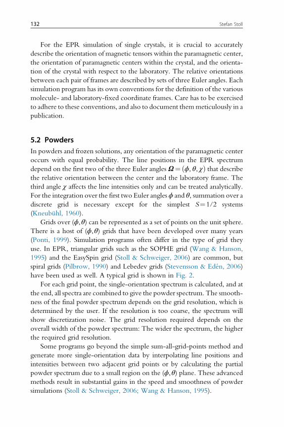
5.2 PowdersIn powders and frozen solutions, any orientation of the paramagnetic center

occurs with equal probability. The line positions in the EPR spectrum

depend on the first two of the three Euler anglesΩ¼ ϕ, θ, χð Þ that describethe relative orientation between the center and the laboratory frame. The

third angle χ affects the line intensities only and can be treated analytically.

For the integration over the first two Euler angles ϕ and θ, summation over a

discrete grid is necessary except for the simplest S¼1/2 systems

(Kneubuhl, 1960).

Grids over (ϕ,θ) can be represented as a set of points on the unit sphere.

There is a host of (ϕ,θ) grids that have been developed over many years

(Ponti, 1999). Simulation programs often differ in the type of grid they

use. In EPR, triangular grids such as the SOPHE grid (Wang & Hanson,

1995) and the EasySpin grid (Stoll & Schweiger, 2006) are common, but

spiral grids (Pilbrow, 1990) and Lebedev grids (Stevensson & Eden, 2006)

have been used as well. A typical grid is shown in Fig. 2.

For each grid point, the single-orientation spectrum is calculated, and at

the end, all spectra are combined to give the powder spectrum. The smooth-

ness of the final powder spectrum depends on the grid resolution, which is

determined by the user. If the resolution is too coarse, the spectrum will

show discretization noise. The grid resolution required depends on the

overall width of the powder spectrum: The wider the spectrum, the higher

the required grid resolution.

Some programs go beyond the simple sum-all-grid-points method and

generate more single-orientation data by interpolating line positions and

intensities between two adjacent grid points or by calculating the partial

powder spectrum due to a small region on the (ϕ,θ) plane. These advancedmethods result in substantial gains in the speed and smoothness of powder

simulations (Stoll & Schweiger, 2006; Wang & Hanson, 1995).

132 Stefan Stoll

The most challenging aspect of powder simulations are looping transi-

tions. These are orientation-dependent transitions between two energy

levels, Ea and Eb, that occur at two fields for a subset of orientations, but

vanish for another subset of orientations because the microwave photon

energy is not able to bridge the energy gap for any field within the sweep

range. At the border between these two sets of orientations, the two reso-

nance lines coalesce in the field sweep and then vanish. Simulation of

looping transitions is challenging because the resonance fields are extremely

sensitive to the orientation of the paramagnetic center in the sense that a

small angle change in ϕ or θ leads to a large change in the line position.

Spherical grids with very high resolution are required in order to get smooth

spectra without artifact features near the coalescence points. Alternatively,

dedicated methods for looping transitions can be used (Gaffney &

Silverstone, 1998). Looping transitions occur in high-spin systems with

zero-field splittings that are on the order of the microwave photon energy.

5.3 Partially Ordered SamplesIn samples such as biological membranes, aligned films, or magnetically

aligned powders, the orientational distribution P(Ω) of spin centers may

deviate from uniform random, as the spin centers can have preferential

alignment along a specific direction or in a specific plane. A nonuniform

P(Ω) is often described using an ordering potential U(Ω), via

P Ωð Þ∝ exp �U Ωð Þ=kBTð Þ with the Boltzmann constant kB and the tem-

perature T. Partial ordering is included in a powder simulation by weighing

the contributions from each spherical grid point according to P(Ω).

Figure 2 A typical spherical (ϕ,θ) grid used in EPR powder simulations (SOPHE grid withN¼ 25). The dots indicate the grid points in polar coordinates corresponding to (ϕ,θ).Due to the inversion symmetry of EPR spectra, only one hemisphere is needed.

133Solid-State CW-EPR Simulations

Orientational distributions based on an ordering potential are extensively

used in the simulation of tumbling paramagnets such as nitroxides using

the stochastic Liouville equation (see “CW-EPR Spectral Simulations:

Slow-motionRegime” byDavid Budil in this volume).WhenU(Ω) is fitted

to spectral data, it is commonly expanded in a linear combination of a few

basis functions such as spherical harmonics YML (ϕ,θ) or Wigner functions

DMKL (ϕ,θ,χ) with low orders L. A high-accuracy determination of the ori-

entational order from experimental EPR spectra beyond these lowest orders

is generally not possible.

6. STRUCTURAL ORDER AND DISORDER

In addition to orientational disorder, the potential presence of struc-

tural disorder also needs to be taken into account in EPR simulations. In a

solid-state sample, the structure of most paramagnetic centers can vary from

site to site. In glasses and frozen solutions, the amorphous molecular envi-

ronment surrounding the paramagnetic center induces structural distortions

in the paramagnetic centers that vary from site to site. Even in crystals, small

site-to-site variations in the geometry are possible. Since molecular structure

determines the SH parameters, a consequence of this site-to-site structural

variability is that SH parameters do not have unique values, but are distrib-

uted. If we label the affected SH parameters as pi, then this means the dis-

tribution P(p1,p2,p3,…) has nonzero width. Such distributions are called

strains. Distributions in g values are termed g strain, distributions in hyperfine

values are called A strain, and distributions in zero-field splitting parameters

are called D strains or D/E strains.

There are two ways to take P(p1,p2,p3,…) into account in a simulation.

First, the simple way is to assume that the distribution is Gaussian along each

parameter and that the distribution is narrow compared to the average value

of the parameter. For example, a Gaussian hyperfine distribution with a

mean of 100 MHz and a standard deviation of 5 MHz would fulfill this

requirement. In this case, the dependence of the EPR resonance field posi-

tion on each SH parameter can be approximated as linear (using the

Hellmann–Feynman theorem), and the effect of the strain can be treated

as simple additional line broadening. This method is usually sufficient for

g distributions in high-field EPR spectra of organic radicals and in standard

EPR spectra of iron complexes (Hagen, Hearshen, Sands, & Dunham,

1985). Correlated distributions of g andA in Cu(II) complexes can be treated

as well (Froncisz & Hyde, 1980). Correlated distributions in the zero-field

134 Stefan Stoll

splitting parameters D and E are used for high-spin systems (Hagen, 2007;

Weisser, Nilges, Sever, & Wilker, 2006).

The second way is more exact but much more expensive: choose an

explicit distribution P(p1,p2,p3,…) of the SH parameters, set up a grid in

this parameter space, explicitly loop over all the grid points, calculate the

corresponding EPR spectra, and then average them using distribution values

as weights. With this, it is possible to quantitatively treat non-Gaussian dis-

tributions and distributions that are very wide. Also, this explicit treatment

can easily take into account correlation between any pair of SH parameters.

This approach is required for modeling the wide distributions of zero-field

splitting parameters that occur in high-spin transition metal complexes.

Often, the simulated spectrum is not very sensitive to the exact distribution

model if the distribution is very wide. Explicit numerical integration over a

grid is of course much more costly in terms of computational time.

7. OTHER LINE BROADENINGS

Beyond orientational and structural disorder, there are several other

potential sources of broadening. Prior to running a simulation, it must be

assessed whether these mechanisms are relevant or not. If they are, they need

to be modeled.

The most common additional source of broadening is due to magnetic

disorder, the site-to-site variation of themagnetic environment even for sites

that are structurally identical. One major source is unresolved hyperfine

couplings to surrounding magnetic nuclei that are not explicitly included

in the SH model. This broadening is typically approximated as Gaussian

in shape and its width is very often anisotropic.

Commonly, the concentration of paramagnetic centers in an EPR sam-

ple is such that it is magnetically dilute, i.e., adjacent paramagnetic centers

are far enough away from each other so that the dipolar through-space mag-

netic coupling between them is negligible compared to the smallest intra-

center interaction. In concentrated samples, this might not be the case,

and significant inter-center coupling can lead to additional broadening in

the EPR spectrum. In solid-state EPR spectra of proteins with the paramag-

netic centers buried in active sites, this is rarely a problem. However, it can

be a problem when studying highly concentrated small-molecule-based

paramagnetic centers. Also, it can occur in a frozen solution if the paramag-

netic centers aggregate during the freezing process.

135Solid-State CW-EPR Simulations

Another potentially important source of broadening in solid-state EPR is

spin relaxation. An EPR transition with a transverse relaxation time constant

of T2 gives rise to a Lorentzian line with a width of T2�1/2π in the frequency

domain and of T2�1/γe in the field domain, where γe is the gyromagnetic

ratio of the electron spin. This additional Lorentzian broadening needs to

be modeled if it is not negligible compared to the other sources of broad-

ening, i.e., when T2 is short and the transverse relaxation rate is fast.

8. EXPERIMENTAL EFFECTS

The nature of the measurement process in standard CW-EPR can

impart certain distortions onto the EPR spectrum. If these distortions are

not avoided during the acquisition of the experimental spectrum, they must

be explicitly included in the simulation. Below, we mention field modula-

tion, saturation, and filtering. Additionally, misalignment of the microwave

phase can lead to absorption/dispersion admixture that needs to be taken

into account as well.

8.1 Field ModulationContinuous-wave EPR uses field modulation combined with phase-

sensitive detection to obtain spectra with good sensitivity. Simulation pro-

grams initially simulate the absorption spectrum without field modulation.

In a second step, the effect of field modulation is then included at one of the

three levels of increasing complexity and generality. (1) If the modulation

amplitude is small relative to the narrowest spectral feature, then it is suffi-

cient to approximate the effect of the field modulation by taking the deriv-

ative of the absorption spectrum with respect to the magnetic field. (2) The

second level of treatment is based on a digital filter in the field domain. In this

approach, the absorption spectrum is convoluted with a lineshape that

approximately represents the effect of the modulation, including over-

modulation if the modulation amplitude is larger than the narrowest spectral

feature. This approach allows the accurate simulation of overmodulated

spectra (Hyde, Pasenkiewicz-Gierula, Jesmanowicz, & Antholine, 1990;

Nielsen, Hustedt, Beth, & Robinson, 2004). (3) Third, the effect of the field

modulation can be taken into account in a full quantitative way that includes

both modulation amplitude and frequency. This entails determining steady-

state solutions of the underlying equations of motions (Bloch equations,

Liouville–von Neumann equation) and is more time-intensive than the

other two methods (Robinson, Mailer, & Reese, 1999). The main benefit

136 Stefan Stoll

of this approach is that it can accurately model the appearance of modulation

side bands. These occur when the modulation frequency is larger than the

inverse linewidth of an EPR absorption line. In practice, this situation hardly

ever occurs in biological EPR, since the lines are generally broad compared

to the standard range of modulation frequencies (up to 100 kHz).

8.2 SaturationIf the microwave power in the experiment is too large, such that the satu-

ration factor 1= 1+ γ2eB21T1T2

� �significantly deviates from 1, then the EPR

spectrum is partially saturated and the lines are broadened. B1 is the strength

of the magnetic component of the microwave at the sample. In this case, the

EPR spectrum is broadened and weakened by an additional factor offfiffiffiffiffiffiffiffiffiffiffiffiffiffiffiffiffiffiffiffiffiffiffiffiffiffiffi1+ γ2eB

21T1T2

p. Since the longitudinal and transverse relaxation times,

T1 and T2, can be orientation dependent, saturation can lead to

orientation-dependent Lorentzian broadening. Generally, it is best to avoid

this situation experimentally by choosing a sufficiently low microwave

power so that an unsaturated spectrum is recorded.

8.3 RC FilteringMany EPR spectrometers have a setting that allows smoothing of the spec-

tral data while they are acquired. Typically, a hardwareRC filter is used. The

user adjusts the time constant of the RC filter to reduce the noise in the

acquired spectrum. If the time constant is too large, the spectrum is

oversmoothed and spectral detail can be lost. Therefore, it is strongly rec-

ommended not to use built-in RC filters and perform all necessary smoo-

thing digitally on the acquired data. Digital postprocessing is preferable,

since it is nondestructive. Nevertheless, if RC filtering was used to acquire

EPR data, it needs to be taken into account in the simulation, especially if an

accurate analysis of the experimental lineshapes is of interest. Digitally, an

RC filter can be applied to a simulated spectrum using a simple convolution

procedure. This requires two inputs, the sampling time TS between two

adjacent points in the spectrum and the RC filter time constant τRC.

9. FITTING

It is the dream of every EPR practitioner to have a simulation program

that is able to automatically fit an experimental EPR spectrum and return the

values of SH parameters of the spin system underlying the spectrum,

137Solid-State CW-EPR Simulations

including their uncertainties. Despite much effort, this is currently not pos-

sible. The many available least-squares fitting algorithms provide tools that

allow the user to find a good fit only if applied properly and within their

capabilities. An absolute prerequisite for a good fit is the choice of a proper

simulation model (spins, SH, broadenings, etc., as discussed in the previous

sections).

With a correct model in hand, the user choices for least-squares fitting

boil down to a few key aspects: First, an adequate objective function needs

to be chosen. Second, a good set of starting parameters and a sufficiently nar-

row search range need to be identified. Third, one or several least-squares

optimization algorithms need to be selected.

9.1 Objective FunctionAn optimization algorithm tries to minimize or maximize an objective func-

tion that measures the quality of the fit between a simulated spectrum ysimand an experimental spectrum yexp. Typically, this is the sum of the squared

deviations (ssd), χ2 p1, p2,…ð Þ¼Pyexp, i� ysim, i p1, p2,…ð Þ� �2

=w2i . The SH

parameters to be varied in the fit are denoted as p1, p2, etc. Weights wi can be

included that depend on the noise level or user-selected range choices.

Unfortunately, this objective function can have many local minima as a

function of the SH parameters, e.g., when the EPR spectrum consists of

many resolved hyperfine peaks. In such cases, other objective functions

can have a much smoother dependence on the SH parameters and are more

likely to work: the ssd of the derivatives, the integrals, the double integrals,

or the Fourier transforms of the experimental and simulated spectra (Stoll,

2011). It is important to explore several of these objective functions.

9.2 Parameter Starting Point and Search RangeThe second crucial choice in a least-squares fitting workflow is the choice of

an appropriate starting point for the SH parameters to be fitted. Most least-

squares fitting algorithms perform best if the minimum of the objective func-

tion lies in the neighborhood of the starting point. Also, it is essential to

restrict the parameter search range as much as physically reasonable to help

convergence. Good starting points can be obtained either from a visual anal-

ysis of the EPR spectrum (if it lends itself to that) or from literature values of

comparable systems. The importance of a good starting point and an ade-

quate limited search region in parameter space cannot be overemphasized.

138 Stefan Stoll

9.3 Fitting AlgorithmLastly, it is important to choose a least-squares fitting algorithm that is ade-

quate for the problem at hand. There are a wide variety of algorithms avail-

able. They differ in many aspects: whether they are (theoretically) able to

locate the global minimum or just walk to the next local minimum, whether

they are deterministic or stochastic, whether they require analytical deriva-

tives of the spectrum with respect to the SH parameters or not, and whether

they can be parallelized or not.

The most popular algorithms are the downhill simplex method due to

Nelder and Mead, and the Levenberg–Marquardt algorithm (Press,

Teukolsky, Vetterling, & Flannery, 2002). The first one is very robust

and has a reasonable chance to escape local minima, although it can be slow.

It is a good default choice for exploring the parameter space. The second one

is an efficient way to locate the local minimum closest to the starting point in

parameter space. Other methods include the Powell method (Hanson et al.,

2004), Monte Carlo methods (Kirste, 1987), simulated annealing (Hustedt,

Smirnov, Laub, Cobb, & Beth, 1997), and genetic algorithms (Filipic &

Strancar, 2001).

As with the objective function, the starting point and the parameter

range, it is best to explore a variety of fitting algorithms for a given problem.

Often, it is useful to combine several algorithms into two-stage hybrid algo-

rithms, where a global method is used to locate the approximate region of

the global minimum, followed by a local and more efficient method that

hones in on the minimum.

10. CONCLUSIONS

Simulation methods for solid-state EPR spectra are well established.

Fairly general simulation programs such as EasySpin (Stoll & Schweiger,

2006) or XSophe (Griffin et al., 1999) are easily available. The broad

range of paramagnetic centers gave rise to a broad range of simulation

methods that are efficient for particular classes of centers. From a user

perspective, it is important to be aware of the wide range of choices avail-

able to be able to identify and pick the correct combination of spin sys-

tem, SH, dynamical regime, theory level, orientational and structural

disorder, broadening model, and experimental distortions. Otherwise,

physically unreasonable spectra are possible, and conclusions can poten-

tially be wrong.

139Solid-State CW-EPR Simulations

In contrast to the systematic workflow for setting up and performing

EPR simulations, the process of using least-squares algorithms to fit a sim-

ulation to experimental data still remains a trial-and-error procedure, for

which there is no silver bullet.

REFERENCESAbragam, A., & Bleaney, B. (1986). Electron paramagnetic resonance of transition ions.NewYork:

Dover.Atherton, N. M. (1993). Principles of electron spin resonance. Chichester: Ellis Horwood.Belford, G. G., Belford, R. L., & Burkhalter, J. F. (1973). Eigenfields: A practical direct cal-

culation of resonance fields and intensities for field-swept fixed-frequency spectrometers.Journal of Magnetic Resonance, 11, 251–265.

Bencini, A., & Gatteschi, D. (1990). Electron paramagnetic resonance of exchange coupled systems.Heidelberg: Springer.

Borras-Almenar, J. J., Clemente-Juan, J. M., Coronado, E., & Tsukerblat, B. S. (2001).MAGPACK a package to calculate the energy levels, bulk magnetic properties, andinelastic neutron scattering spectra of high nuclearity spin clusters. Journal of Computa-tional Chemistry, 22(9), 985–991.

Chilton, N. F., Anderson, R. P., Turner, L. D., Soncini, A., & Murray, K. S. (2013). PHI:A powerful new program for the analysis of anisotropic monomeric and exchange-coupled polynuclear d- and f-block complexes. Journal of Computational Chemistry, 34,1164–1175.

Claridge, R. F. C., Tennant, W. C., & McGavin, D. G. (1997). X-band EPR of Fe3+/CaWO4 at 10 K: Evidence for large magnitude high spin Zeeman interactions. Journalof Physics and Chemistry of Solids, 58, 813–820.

Filipic, B., & Strancar, J. (2001). Tuning EPR spectral parameters with a genetic algorithm.Applied Soft Computing, 1, 83–90.

Froncisz, W., & Hyde, J. S. (1980). Broadening by strains of lines in the g-parallel region ofCu2+ EPR spectra. The Journal of Chemical Physics, 73, 3123–3131.

Gaffney, B. J., & Silverstone, H. J. (1998). Simulation methods for looping transitions. Journalof Magnetic Resonance, 134, 57–66.

Golombek, A. P., & Hendrich, M. P. (2003). Quantitative analysis of dinuclearmanganese(II) EPR spectra. Journal of Magnetic Resonance, 165, 33–48.

Griffin, M., Muys, A., Noble, C., Wang, D., Eldershaw, C., Gates, K. E., et al. (1999).XSophe, a computer simulation software suite for the analysis of electron paramagneticresonance spectra. Molecular Physics Reports, 26, 60–84.

Hagen, W. R. (2007). Wide zero field interaction distributions in the high-field EPR ofmetalloproteins. Molecular Physics, 105, 2031–2039.

Hagen,W.R., Hearshen, D. O., Sands, R. H., &Dunham,W.R. (1985). A statistical theoryfor powder EPR in distributed systems. Journal of Magnetic Resonance, 61, 220–232.

Hanson, G. R., Gates, K. E., Noble, C. J., Griffin, M., Mitchell, A., & Benson, S. (2004).XSophe-Sophe-XeprView: A computer simulation software suite (v. 1.1.3) for the anal-ysis of continuous wave EPR spectra. Journal of Inorganic Biochemistry, 98, 903–916.

Harris, E. A., &Owen, J. (1963). Biquadratic exchange betweenMn2+ ions inMgO. PhysicalReview Letters, 11(1), 9–10.

Heinzer, J. (1971). Fast computation of exchange-broadened isotropic E.S.R. spectra.Molec-ular Physics, 22(1), 167–177.

Hudson, A., & Luckhurst, G. R. (1969). The electron resonance line shapes of radicals insolution. Chemical Reviews, 69(2), 191–225.

140 Stefan Stoll

Hustedt, E. J., Smirnov, A. I., Laub, C. F., Cobb, C. E., & Beth, A. H. (1997). Moleculardistances from dipolar coupled spin-labels: The global analysis of multifrequency contin-uous wave electron paramagnetic resonance data. Biophysical Journal, 74, 1861–1877.

Hyde, J. S., Pasenkiewicz-Gierula, M., Jesmanowicz, A., & Antholine,W. E. (1990). Pseudofield modulation in EPR spectroscopy. Applied Magnetic Resonance, 1, 483–496.

Iwasaki, M. (1974). Second-order perturbation treatment of the general spin Hamiltonian inan arbitrary coordinate system. Journal of Magnetic Resonance, 16, 417–423.

Kirste, B. (1987). Least-squares fitting of EPR spectra by Monte Carlo methods. Journal ofMagnetic Resonance, 73, 213–224.

Kneubuhl, F. K. (1960). Line shapes of electron paramagnetic resonance signals producedby powders, glasses, and viscous liquids. The Journal of Chemical Physics, 33(4),1074–1078.

Mabbs, F. E., & Collison, D. (1992). Electron paramagnetic resonance of d transition metal com-pounds. Amsterdam: Elsevier.

Mombourquette,M. J., Tennant,W.C., &Weil, J. A. (1986). EPR study of Fe3+ in α-quartz.The Journal of Chemical Physics, 85(1), 68–79.

Neese, F. (2004). Zero-field splitting. In M. Kaupp, M. Buhl, & V. G. Malkin (Eds.),Calculation of EPR and NMR parameters (pp. 541–566). Weinheim: Wiley-VCH.

Nielsen, R. D., Hustedt, E. J., Beth, A. H., & Robinson, B. H. (2004). Formulation ofZeeman modulation as a signal filter. Journal of Magnetic Resonance, 170, 345–371.

Pake, G. E., & Estle, T. L. (1973). The physical principles of electron paramagnetic resonance.Reading, MA: Benjamin.

Patchkovskii, S., & Schreckenbach, G. (2004). Calculation of g-tensors with density func-tional theory. In M. Kaupp, M. Buhl, & V. G. Malkin (Eds.), Calculation of NMR andEPR parameters (pp. 505–532). Weinheim: Wiley-VCH.

Pilbrow, J. R. (1990). Transition ion electron paramagnetic resonance. Oxford: Clarendon Press.Piligkos, S., Weihe, H., Bill, E., Neese, F., El Mkami, H., Smith, G. M., et al. (2009). EPR

spectroscopy of a family of CrIII7MnII (M ¼ Cd, Zn, Mn, Ni) “wheels”: Studies of iso-structural compounds with different spin ground states. Chemistry - A European Journal,15, 3152–3167.

Ponti, A. (1999). Simulation of magnetic resonance static powder lineshapes: A quantitativeassessment of spherical codes. Journal of Magnetic Resonance, 138, 288–297.

Press, W. H., Teukolsky, S. A., Vetterling, W. T., & Flannery, B. P. (2002).Numerical recipesin C (2nd ed.). New York: Cambridge University Press.

Robinson, B. H., Mailer, C., & Reese, A. W. (1999). Linewidth analysis of spin labels inliquids. Journal of Magnetic Resonance, 138, 199–209.

Rudowicz, C., & Karbowiak, M. (2015). Disentangling intricate web of interrelated notionsat the interface between the physical (crystal field) Hamiltonians and the effective (spin)Hamiltonians. Coordination Chemistry Reviews, 287, 28–63.

Shaw, J. L., Wolowska, J., Collison, D., Howard, J. A. K., McInnes, E. J. L., McMaster, J.,et al. (2006). Redox non-innocence of thioether macrocycles: Elucidation of the elec-tronic structures of mononuclear complexes of gold(II) and silver(II). Journal of theAmerican Chemical Society, 128, 13827–13839.

Speldrich, M., Schilder, H., Lueken, H., & Kogerler, P. (2011). A computational frameworkfor magnetic polyoxometalates and molecular spin structures: CONDON 2.0. IsraelJournal of Chemistry, 51(2), 215–227.

Stevensson, B., & Eden, M. (2006). Efficient orientational averaging by the extension ofLebedev grids via regularized octahedral symmetry expansion. Journal of MagneticResonance, 181, 162–176.

Stoll, S. (2011). High-field EPR of bioorganic radicals. In B. C. Gilbert, D. M. Murphy, &V. Chechik (Eds.), Vol. 22. Electron paramagnetic resonance (pp. 107–154). Cambridge:Royal Society of Chemistry.

141Solid-State CW-EPR Simulations

Stoll, S. (2014). Computational modeling and least-squares fitting of EPR spectra.In S. K. Misra (Ed.), Multifrequency electron paramagnetic resonance (pp. 69–138).Weinheim: Wiley-VCH.

Stoll, S., & Schweiger, A. (2003). An adaptive method for computing resonance fields forcontinuous-wave EPR spectra. Chemical Physics Letters, 380, 464–470.

Stoll, S., & Schweiger, A. (2006). EasySpin, a comprehensive software package for spectralsimulation and analysis in EPR. Journal of Magnetic Resonance, 178, 42–55.

Wang, D., & Hanson, G. R. (1995). A new method for simulating randomly oriented pow-der spectra in magnetic resonance: The Sydney opera house (SOPHE) method. Journal ofMagnetic Resonance. Series A, 117, 1–8.

Weil, J. A., & Bolton, J. R. (2007). Electron paramagnetic resonance. Elementary theory and practicalapplications. Hoboken, NJ: Wiley.

Weil, J. A., Buch, T., & Clapp, J. E. (1973). Crystal point group symmetry and microscopictensor properties in magnetic resonance spectroscopy. Advances in Magnetic Resonance, 6,183–257.

Weisser, J. T., Nilges, M. J., Sever, M. J., &Wilker, J. J. (2006). EPR investigation and spec-tral simulations of iron-catecholate complexes and iron-peptide models of marine adhe-sive cross-links. Inorganic Chemistry, 45, 7736–7747.

Zalibera, M., Jalilov, A. S., Stoll, S., Guzei, I. A., Gescheidt, G., & Nelsen, S. F. (2013).Monotrimethylene-bridged Bis-p-pheneylenediamine radical cations and dications:Spin states, conformations, and dynamics. The Journal of Physical Chemistry. A, 117,1439–1448.

142 Stefan Stoll