Full Terms & Conditions of access and use can be found athttps://www.tandfonline.com/action/journalInformation?journalCode=hsem20

Structural Equation Modeling: A Multidisciplinary Journal

ISSN: 1070-5511 (Print) 1532-8007 (Online) Journal homepage: https://www.tandfonline.com/loi/hsem20

Cutoff criteria for fit indexes in covariancestructure analysis: Conventional criteria versusnew alternatives

Li‐tze Hu & Peter M. Bentler

To cite this article: Li‐tze Hu & Peter M. Bentler (1999) Cutoff criteria for fit indexes in covariancestructure analysis: Conventional criteria versus new alternatives, Structural Equation Modeling: AMultidisciplinary Journal, 6:1, 1-55, DOI: 10.1080/10705519909540118

To link to this article: https://doi.org/10.1080/10705519909540118

Published online: 03 Nov 2009.

Submit your article to this journal

Article views: 49583

View related articles

Citing articles: 38842 View citing articles

STRUCTURAL EQUATION MODELING, 6(1), 1-55Copyright © 1999, Lawrence Erlbaum Associates, Inc.

Cutoff Criteria for Fit Indexes inCovariance Structure Analysis:Conventional Criteria Versus

New Alternatives

Li-tze HuDepartment of Psychology

University of California, Santa Cruz

Peter M. BentlerDepartment of Psychology

University of California, Los Angeles

This article examines the adequacy of the "rules of thumb" conventional cutoff crite-ria and several new alternatives for various fit indexes used to evaluate model fit inpractice. Using a 2-index presentation strategy, which includes using the maximumlikelihood (ML)-based standardized root mean squared residual (SRMR) and supple-menting it with either Tucker-Lewis Index (TLI), Bollen's (1989) Fit Index (BL89),Relative Noncentrality Index (RNI), Comparative Fit Index (CFI), Gamma Hat, Mc-Donald's Centrality Index (Mc), or root mean squared error of approximation(RMSEA), various combinations of cutoff values from selected ranges of cutoff crite-ria for the ML-based SRMR and a given supplemental fit index were used to calculaterejection rates for various types of true-population and misspecified models; that is,models with misspecified factor covariance(s) and models with misspecified factorloading(s). The results suggest that, for the ML method, a cutoff value close to .95 forTLI, BL89, CFI, RNI, and Gamma Hat; a cutoff value close to .90 for Mc; a cutoffvalue close to .08 for SRMR; and a cutoff value close to .06 for RMSEA are neededbefore we can conclude that there is a relatively good fit between the hypothesizedmodel and the observed data. Furthermore, the 2-index presentation strategy is re-quired to reject reasonable proportions of various types of true-population andmisspecified models. Finally, using the proposed cutoff criteria, the ML-based TLI,Mc, and RMSEA tend to overreject true-population models at small sample size andthus are less preferable when sample size is small.

Requests for reprints should be sent to Li-tze Hu, Department of Psychology, University of Califor-nia, Santa Cruz, CA 95064.

2 HUANDBENTLER

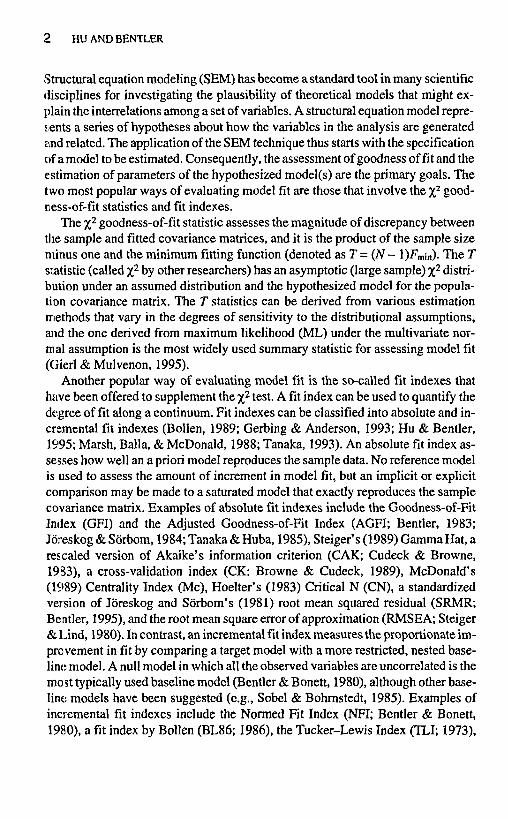
Structural equation modeling (SEM) has become a standard tool in many scientificdisciplines for investigating the plausibility of theoretical models that might ex-plain the interrelations among a set of variables. A structural equation model repre-sents a series of hypotheses about how the variables in the analysis are generatedand related. The application of the SEM technique thus starts with the specificationof amodel to be estimated. Consequently, the assessment of goodness of fit and theestimation of parameters of the hypothesized model(s) are the primary goals. Thetwo most popular ways of evaluating model fit are those that involve the X2 good-ness-of-fit statistics and fit indexes.

The x2 goodness-of-fit statistic assesses the magnitude of discrepancy betweenthe sample and fitted covariance matrices, and it is the product of the sample sizeminus one and the minimum fitting function (denoted asT=(N- l)Fmn)- The Tstatistic (called %2 by other researchers) has an asymptotic (large sample) %2 distri-bution under an assumed distribution and the hypothesized model for the popula-tion covariance matrix. The T statistics can be derived from various estimationmethods that vary in the degrees of sensitivity to the distributional assumptions,and the one derived from maximum likelihood (ML) under the multivariate nor-mal assumption is the most widely used summary statistic for assessing model fit(Gierl & Mulvenon, 1995).

Another popular way of evaluating model fit is the so-called fit indexes thathave been offered to supplement the %2 test. A fit index can be used to quantify thedegree of fit along a continuum. Fit indexes can be classified into absolute and in-cremental fit indexes (Bollen, 1989; Gerbing & Anderson, 1993; Hu & Bentler,1995; Marsh, Balla, & McDonald, 1988; Tanaka, 1993). An absolute fit index as-sesses how well an a priori model reproduces the sample data. No reference modelis used to assess the amount of increment in model fit, but an implicit or explicitcomparison may be made to a saturated model that exactly reproduces the samplecovariance matrix. Examples of absolute fit indexes include the Goodness-of-FitIndex (GFI) and the Adjusted Goodness-of-Fit Index (AGFI; Bentler, 1983;Joreskog & Sorbom, 1984; Tanaka & Huba, 1985), Steiger's (1989) Gamma Hat, arescaled version of Akaike's information criterion (CAK; Cudeck & Browne,1933), a cross-validation index (CK: Browne & Cudeck, 1989), McDonald's(1989) Centrality Index (Me), Hoelter's (1983) Critical N (CN), a standardizedversion of Joreskog and Sorbom's (1981) root mean squared residual (SRMR;Bentler, 1995), and the root mean square error of approximation (RMSEA; Steiger& Lind, 1980). In contrast, an incremental fit index measures the proportionate im-provement in fit by comparing a target model with a more restricted, nested base-line model. A null model in which all the observed variables are uncorrelated is themost typically used baseline model (Bentler & Bonett, 1980), although other base-line, models have been suggested (e.g., Sobel & Bohrnstedt, 1985). Examples ofincremental fit indexes include the Normed Fit Index (NFI; Bentler & Bonett,1980), a fit index by Bollen (BL86; 1986), the Tucker-Lewis Index (TLI; 1973),

CUTOFF CRITERIA AND FIT INDEXES 3

an index developed by Bollen (BL89; 1989), Bender's (1989, 1990) and McDon-ald and Marsh's (1990) Relative Noncentrality Index (RNI), and Bender's Com-parative Fit Index (CFI). See Table 1 for some of the formulas.

As noted by Bentler and Bonett (1980), fit indexes were designed to avoid someof the problems of sample size and distributional misspecification associated withthe conventional overall test of fit (the %2 statistic) in the evaluation of a model. How-ever, this promising claim that fit indexes would more unambiguously point tomodel adequacy as compared to the %2 test has little empirical support. Thus, twopressing issues that are relevant to proper applications of fit indexes for model evalu-

Formula

TABLE 1Formulas and Descriptions for Incremental and Absolute Fit Indexes

Description

Incremental fit indexesTLI (or NNFI) = [(J*ldfB) - {TJdBVKTJdfc) - 1]

BL89 (or IFI) = (rB - TT)/(.TB - dfi)

RNI = [(71, - <//„) - (TT - dfy)]/(TB - dfB)

CFI = I - max[(7V - dfT), 0]/max[(rT - dfT), (TB - dfB), 0]

Absolute Fit IndexesGamma Hat =pl[p + 2[{TT - dfT)/(N - 1)])

Me = expH/2[(rT-d/T)/(/V- 1)]}

jSRMR =

RMSEA = JPD I dfT, where Fo = max[(TT - dh)l(N - 1), 0]

Nonnormed (can fall outside the0-1 range). Compensates forthe effect of modelcomplexity.

Nonnormed. Compensates forthe effect of modelcomplexity.

Nonnormed. Noncentrality-based.

Normed (has a 0-1 range).Noncentrality-based.

Has a known distribution.Noncentrality-based.

Noncentrality-based. Typicallyhas the 0-1 range (but it mayexceed 1).

Standardized root mean squaredresidual.

Has a known distribution.Compensates for the effect ofmodel complexity.Noncentrality-based.

Note. TT = T statistic for the target model; dfr = df for the target model; TB = T statistic for thebaseline model; dfB = df for the baseline model; p = number of observed variables; Sy = observedcovariances; a,j = reproduced covariances; sa and s^ are the observed standard deviations; TLI =Tucker-Lewis Index; NNFI = Nonnormed Fit Index; BL89 = Bollen's Fit Index (1989); IFI =Incremental Fit Index; RNI = Relative Noncentrality Index; CFI = Comparative Fit Index; Me =McDonald's Centrality Index; SRMR = standardized root mean squared residual; RMSEA = root meansquared error of approximation.

4 HU AND BENTLER

ation have become the primary concern of many researchers. The first pressing issueis determination of adequacy of fit indexes under various data and model conditionsoften encountered in practice. These conditions include sensitivity of fit index tomodel misspecification, small sample bias, estimation method effect, effects of vio-lation of normality and independence, and bias of fit indexes resulting from modelcomplexity. The second pressing issue is the selection of the "rules of thumb" con-ventional cutoff criteria for given fit indexes used to evaluate model fit.

Although the first issue has been addressed by many researchers (e.g., Akaike,1987; Ding, Velicer, & Harlow, 1995; Hu & Bentler, in press; James, Mulaik, &Brett, 1982; La Du & Tanaka, 1989; Marsh & Balla, 1994; Marsh, Balla, & Hau,1996; Steiger&Lind, 1980; Sugawara&MacCallum, 1993;Tanaka, 1987),thesec-ond issue has rarely been studied empirically (e.g., Marsh & Hau, 1996). Conse-quently, researchers often question the adequacy of these conventional cutoffcriteria due to the lack of empirical evidence and compelling rationale for these rulesof thumb. For example, Marsh (1995) suggested that although researchers typicallyinterpret values greater than .90 as acceptable for incremental fit indexes (e.g., RNI),no compelling rationale for this rule of thumb has been provided. Mulaik recentlysuggested raising the rule of thumb minimum standard for the CFI from .90 to .95 toreduce the number of severely misspecified models that are considered acceptablebased on the .90 criterion (e.g., Carlson & Mulaik, 1993; cf. Rigdon, 1996). Usingdata simulated from a known population simplex model (i.e., a model in which thesame latent construct is evaluated with the same three indicators on each of three oc-casions), Marsh and Hau (1996) evaluated the behavior of a wide variety of indexesof fit and decision rules based on these indexes in comparing parsimonious andnonparsimonious (with correlated uniqueness) simplex models. Their results re-vealed that decision rules such as RMSEA < .05, NFI (Relative Fit Index [RFI],Nonnormed Fit Index [NNFI], Incremental Fit Index [IFI], RNI, CFI, or GFI) > .90,and parsimony indexes > .80 may be useful in some solutions but they often lead toinappropriate decisions in other solutions (e.g., decision rules forthe acceptability ofth« parsimonious model often lead to inappropriate decisions), and should be con-sidered only as rules of thumb. In addition, decision rules based on the comparison ofthe parsimonious and nonparsimonious models were more likely to result in the ap-propriate acceptance of the nonparsimonious model.

This discussion undoubtedly points to the need for identifying adequate rule ofthumb cutoff criteria for fit indexes used to evaluate goodness of fit of hypothe-sized models. In this study, we evaluate the adequacy of the rules of thumb con-ventional cutoff criteria and other alternative criteria for various fit indexes.Although other decision rules (e.g., the selection of either the largest or smallestvalues for fit indexes incorporating parsimony or estimation penalties) have beenproposed for fit indexes used to compare the fit of competing (i.e., nested) models(e.g., Marsh & Hau, 1996), our study only evaluates cutoff criteria under a priorimodels.

CUTOFF CRITERIA AND FIT INDEXES 5

DEALING WITH A PRESSING ISSUE INASSESSING FIT BY FIT INDEXES

Hu and Bentler (in press) evaluated the sensitivity of various types of incremen-tal fit indexes and absolute fit indexes derived from ML, generalized leastsquares (GLS), and asymptotically distribution-free (ADF) estimators tounderparameterized model misspecification. They also examined adequacy ofthese indexes when (a) distributional, (b) assumed independence, and (c) asymp-totic sample size requirements were violated. Their results include the following.First, most of the ML-based fit indexes outperform those obtained from GLSand ADF, and should be preferred indicators for evaluating model fit. Second,NFI, BL86, CAK, CK, CN, GFI, and AGFI performed poorly and are not rec-ommended for evaluating model fit. Third, the ML-based SRMR is the mostsensitive index to models with misspecified factor covariance(s) or latent struc-ture^), and the ML-based TLI, BL89, RNI, CFI, Gamma Hat, Me, and RMSEAare the most sensitive indexes to models with misspecified factor loadings.Fourth, on the basis of a correlation matrix among the ML-based fit indexes ob-tained to determine which fit indexes might behave similarly along three majordimensions (sample size, distribution, and model misspecification), two majorclusters of correlated fit indexes were identified. NFI, BL86, GFI, AGFI, CAK,and CK were clustered with high correlations. Another cluster of highintercorrelations included TLI, BL89, RNI, CFI, Me, and RMSEA. SRMR per-formed least similarly to the other ML-based fit indexes. A series of analyses ofvariance using sample size, distribution, and model misspecification as inde-pendent variables lend further support to the behavioral pattern of these indexesidentified from the correlation matrix. The findings suggested that there wasvariation of performance among the recommended fit indexes, and thus atwo-index presentation strategy that includes using the ML-based SRMR, andsupplementing it with the ML-based TLI, BL89, RNI, CFI, Gamma Hat, Me, orRMSEA was proposed to distinguish good models from poor ones that includemodels with misspecified factor covariance(s), factor loading(s), or both.

Given that a researcher does use recommended fit indexes (Hu & Bentler, inpress) to evaluate a model, what rule of thumb cutoff values should be considered?An adequate cutoff criterion for a given fit index should result in minimum Type Ierror rate (i.e., the probability of rejecting the null hypothesis when it is true) andType II error rate (i.e., the probability of accepting the null hypothesis when it isfalse). To address this pressing issue, our study evaluates the adequacy of rules ofthumb conventional cutoff criteria (e.g., Bentler, 1989; Bentler & Bonett, 1980)and other alternative criteria for the ML-based TLI, BL89, RNI, CFI, Gamma Hat,Me, RMSEA, and SRMR.

First, considering any model with a fit index above .9 as acceptable (e.g., Bentler,1989; Bentler & Bonett, 1980) and any one with an index below this value as unac-

(5 HU AND BENTLER

ceptable, we evaluate the rejection rates for simple (i.e., models with misspecifiedfactor covariance(s)) and complex (i.e., models with misspecified factor loading(s))true-population/misspecified models for the ML-based TLI, BL89, RNI, CFI,CJamma Hat, and Me. A cutoff value of .05 was used for SRMR and RMSEA. Steiger(1989), Browne and Mels (1990), and Browne and Cudeck (1993) recommendedthat values of RMSEA less than .05 be considered as indicative of close fit. Browneand Cudeck also suggested that values in the range of .05 to .08 indicate fair fit, andthat values greater than .10 indicate poor fit. MacCallum, Browne, and Sugawara(1996) considered values in the range of .08 to. 10 to indicate mediocre fit. These pre-li minary analyses will allow us to determine Type I error and Type II error rates un-der rules of thumb conventional cutoff criteria for these ML-based fit indexes.Second, based on the preliminary analyses and the two-index presentation strategyproposed by Hu and Bentler (in press), various combinations of cutoff values fromselected ranges of cutoff values for the ML-based SRMR and a given supplementalfit index (i.e., the ML-based TLI, BL89, RNI, CFI, Gamma Hat, Me, or RMSEA)were used to calculate rejection rates for simple and complextrue-population/misspecified models. For example, rejection rates for differenttypes of models were calculated by the combinational rule of SRMR > .08 andRMSEA>.05,SRMR>.08andRMSEA>.06,SRMR>.08andCFI<.95,orSRMR> .08 and CFI < .96. First, we compare the performance of the rules of thumb conven-tional and several new alternative cutoff values for the ML-based TLI, BL89, RNI,CH, Gamma Hat, Me, SRMR, and RMSEA. The adequacy of our proposed combi-national rules is then evaluated by comparing (a) Type I and Type II error rates forsimple and complex true-population models and misspecified models (I and II) and(b) the sums and average values of sums of Type I and Type II error rates for simpleand complex true-population models and misspecified models (I).

METHOD

Study Design

Two types of models (called simple and complex here) are used to generate mea-sured variables under various conditions on the common factors and unique vari-ate s (cf. Hu & Bentler, in press). Simple and complex models are both confirmatoryfactor-analytic models based on 15 observed variables with three common factors.The factor-loading matrix (transposed) L' for the simple model has the followingstructure:

.70 .70 .75 .80 .80 .00 .00 .00 .00 .00 .00 .00 .00 .00 .00

.00 .00 .00 .00 .00 .70 .70 .75 .80 .80 .00 .00 .00 .00 .00

.00 .00 .00 .00 .00 .00 .00 .00 .00 .00 .70 .70 .75 .80 .80

CUTOFF CRITERIA AND FIT INDEXES 7

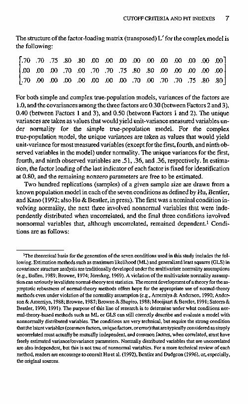
The structure of the factor-loading matrix (transposed) L' for the complex model isthe following:

'.70 .70 .75 .80 .80 .00 .00 .00 .00 .00 .00 .00 .00 .00 .00

.00 .00 .00 .70 .00 .70 .70 .75 .80 .80 .00 .00 .00 .00 .00

.70 .00 .00 .00 .00 .00 .00 .00 .70 .00 .70 .70 .75 .80 .80

For both simple and complex true-population models, variances of the factors are1.0, and the covariances among the three factors are 0.30 (between Factors 2 and 3),0.40 (between Factors 1 and 3), and 0.50 (between Factors 1 and 2). The uniquevariances are taken as values that would yield unit-variance measured variables un-der normality for the simple true-population model. For the complextrue-population model, the unique variances are taken as values that would yieldunit-variance for most measured variables (except for the first, fourth, and ninth ob-served variables in the model) under normality. The unique variances for the first,fourth, and ninth observed variables are .51, .36, and .36, respectively. In estima-tion, the factor loading of the last indicator of each factor is fixed for identificationat 0.80, and the remaining nonzero parameters are free to be estimated.

Two hundred replications (samples) of a given sample size are drawn from aknown population model in each of the seven conditions as defined by Hu, Bentler,and Kano (1992; also Hu & Bentler, in press). The first was a nominal condition in-volving normality, the next three involved nonnormal variables that were inde-pendently distributed when uncorrelated, and the final three conditions involvednonnormal variables that, although uncorrelated, remained dependent.1 Condi-tions are as follows:

1The theoretical basis for the generation of the seven conditions used in this study includes the fol-lowing. Estimation methods such as maximum likelihood (ML) and generalized least squares (GLS) incovariance structure analysis are traditionally developed under the multivariate normality assumptions(e.g., Bollen, 1989; Browne, 1974; Jöreskog, 1969). A violation of the multivariate normality assump-tion can seriously invalidate normal-theory test statistics. The recent development of a theory for the as-ymptotic robustness of normal-theory methods offers hope for the appropriate use of normal-theorymethods even under violation of the normality assumption (e.g., Amemiya & Anderson, 1990; Ander-son & Amemiya, 1988; Browne, 1987; Browne & Shapiro, 1988; Mooijaart & Bentler, 1991;Satorra&Bentler, 1990, 1991). The purpose of this line of research is to determine under what conditions nor-mal-theory-based methods such as ML or GLS can still correctly describe and evaluate a model withnonnormally distributed variables. The conditions are very technical, but require the strong conditionthat the latent variables (common factors, unique factors, or error) that are typically considered as simplyuncorrelated must actually be mutually independent, and common factors, when correlated, must havefreely estimated variance/covariance parameters. Normally distributed variables that are uncorrelatedare also independent, but this is not true of nonnormal variables. For a more technical review of eachmethod, readers are encourage to consult Hu et al. (1992), Bentler and Dudgeon (1996), or, especially,the original sources.

« HU AND BENTLER

1. The factors and errors and hence measured variables are multivariate nor-mally distributed.

2. Nonnormal factors and errors, when uncorrelated, are independent, but as-ymptotic robustness theory does not hold because the covariances of com-mon factors are not free parameters.

3. Nonnormal factors and errors that are independent but not multivariate nor-mally distributed.

4. The errors and hence the measured variables are not multivariate normallydistributed.

5. An elliptical distribution in which factors and errors are uncorrelated butdependent on each other.

6. The errors and hence the measured variables are not multivariate normallydistributed and both factors and errors are uncorrelated but dependent oneach other.

7. Nonnormal factors and errors that are uncorrelated but dependent on eachother.

These seven conditions are created through various distributional specifications onthe common and (unique) error factors. In Condition 1, both common and error fac-tois are normally distributed, with no excess kurtosis. The true kurtoses for thenonnormal common factors in Conditions 2 and 3 are —1.0, 2.0, and 5.0. The truekurtoses of the unique variates for Conditions 2 through 4, in which the errors arenonnormal, are-1.0,0.5,2.5,4.5,6.5, -1.0,1.0,3.0,5.0,7.0,-0.5,1.5,3.5,5.5, and7.5. In Conditions 5 through 7, the factors and error variates are divided by a ran-dom variable z = [%2 (5)1 / v3 that is distributed independently of the original

common and unique factors. As a consequence of this division, the factors and er-rors are uncorrelated but dependent on each other. Because of the dependence, as-ymptotic robustness of normal-theory statistics is not to be expected under Condi-tions 5 through 7. Using modified simulation procedures in EQS (Bentler & Wu,1995a) and SAS programs2 (SAS, 1993), the various fit indexes based on MLmethod are computed in each sample.

Model Specification and Procedure

For each type of model (i.e., simple or complex), one true-population model andtwo misspecified models are used to examine the adequacy of rules of thumb con-ventional and several new alternative cutoff values for fit indexes used for modelevaluation.

2BL89, Relative Noncentrality Index, Gamma Hat, McDonald's Centrality Index, and root meansquansd error of approximation were computed by SAS programs.

CUTOFF CRITERIA AND FIT INDEXES 9

True-population model. For the true-population model, the adequacy ofconventional cutoff criteria for the ML-based fit indexes are examined. A sample ofsize N was drawn from the population and the model was estimated in that sample.The results were saved, and the process was repeated for 200 replications. This pro-cess was repeated for sample sizes N = 150,250,500,1,000,2,500, and 5,000. Inall, there were 7 x 6 x 200 (Conditions x Sample Sizes x Replications)=8,400 sam-ples. The fit indexes based on ML method were calculated for each of these sam-ples. This procedure was conducted for simple and complex models separately.

Misspecified models. Although both underparameterized and over-parameterized models have been considered as incorrectly specified models, ourstudy only examines the adequacy of conventional cutoff criteria for fit indexes de-rived from underparameterized models, because overparameterized models havezero population noncentrality (e.g., MacCallum et al., 1996; Satorra & Saris, 1985).For a simple model, the covariances among the three factors in the correctly specifiedpopulation model (true-population model) are nonzeros. The covariance betweenFactors 1 and 2 was fixed to zero for the first misspecified model (simplemisspecified model 1). The covariances between Factors 1 and 2 and between Fac-tors 1 and 3 were fixed to zeros for the second misspecified model (simplemisspecified model 2). For a complex model, three observed variables loaded on twofactors in the true-population model: (a) the first observed variable loaded on Factors1 and 3, (b) the fourth observed variable loaded on Factors 1 and 2, and (c) the ninthobserved variable loaded on Factors 2 and 3. In the first misspecified model (complexmisspecified model 1), the first observed variable only loaded on Factor 1, whereasthe rest of the model specification remained the same as the complex true-populationmodel. In the second misspecified model (complex misspecified model 2), the firstand fourth observed variables only loaded on one single factor (both on Factor 1).

Using the design parameters specified in either the simple or complextrue-population model, a sample of size N was drawn from the population and eachof the misspecified models was estimated in that sample. The results were saved,and the process was repeated for 200 replications. This process was repeated forsix sample sizes. For each misspecified model, there were 7 (conditions) x 6 (sam-ple sizes) x 200 (replications) = 8,400 samples. The fit indexes based on the MLmethod were calculated for each of these samples.

RESULTS

Preliminary Comparison Between Conventional andAlternative Cutoff Values for the ML-Based Fit Indexes

The tendency for committing Type I error of the ML-based fit indexes was evalu-ated based on the overrejection rates obtained for the simple and complex

10 HUANDBENTLER

Irue-population models under various conditions. The tendency for committingType II error was evaluated based on the underrejection rates obtained for varioussimple and complex misspecified models. Note that our purpose here is to evaluateadequacy of the rules of thumb conventional cutoff values discussed earlier. Theseare arbitrary in nature for various fit indexes (e.g., Bentler & Bonett, 1980; Browne& Cudeck, 1993; MacCallum et al., 1996; Steiger, 1989).

For preliminary analyses, the original six sample sizes (TV = 150, 250, 500,1,000,2,500, and 5,000) across Conditions 1 through 7 were further classified intotliree categories: N < 250, N = 500, and 1,000 < N. Using various cutoff values, re-jection rates for each of the recommended ML-based fit indexes under each type ofthe simple or complex true-population and misspecified models were calculatedacross seven distributional conditions and tabulated for the three sample sizes. Ta-bles 2 and 3 display the rejection rates based on the ML-based TLI, BL89, RNI,CFI, Gamma Hat, SRMR, and RMSEA under the selected cutoff criteria for sim-ple and complex true-population models and misspecified models (I and II).

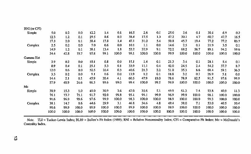
With a cutoff value of .90 and across three sample size categories, BL89, RNI,and CFI only rejected 0.1% to 54.4% of all types of misspecified models, whereasTLI rejected about 0.1% to 27.6% of all types of misspecified models, except thecomplex misspecified models (II) (81.8%—97.5% were rejected by TLI). Substan-tial Type II error rates were observed with a cutoff value of .90, and thus a cutoffvalue greater than .90 is required to reject adequate proportions of misspecifiedmodels. Using a cutoff value of .93 or .94, TLI, BL89, RNI, and CFI rejected lessthan 50% of simple misspecified models (I and II) and complex misspecified mod-els (I) in most conditions. More than 95% of the complex misspecified models (II)were rejected by these cutoff values. With a cutoff value of .95 and N < 500, onlyabout 29.8% to 71.5% of simple misspecified models (I and II) were rejected, andabout 67.4% to 92.6% of complex misspecified models (I) and 99.9% to 100% ofthe complex misspecified models (II) were rejected. With a cutoff value of .95 andNl'. 1,000, only 4.6% to 57.6% of simple misspecified models (I and II) were re-jected, and about 56.7% to 99.4% of complex misspecified models (I) and 100% ofcomplex misspecified models (II) were rejected. With a cutoff value of .96, theyrejected less than 50% (except TLI) of simple misspecified models (I) in most con-ditions, 76.3% to 99% of simple misspecified models (II), 88.5% to 99.6% ofcomplex misspecified models (I), and 100% of complex misspecified models (II).With a cutoff value of .90, Gamma Hat rejected 0.1% to 12% of simplemisspecified models (I and II), 0.1 % to 14.4% of complex misspecified models (I),and 24.6% to 57.9% of complex misspecified models (II). With a cutoff value of.93 or .94, Gamma Hat rejected 0.1% to 40.6% of simple misspecified models (Iand II), 4.1% to 60.5% of complex misspecified models (I), and 96.3% to 100% ofcomplex misspecified models (II). With a cutoff value of .95, Gamma Hat rejected2.4% to 51% of simple misspecified models (I and II) and 78.6% to 100% of com-plex misspecified models (I and II). With a cutoff value of .96, Gamma Hat re-

CUTOFF CRITERIA AND FIT INDEXES 11

jected 8.7% to 68.4% of simple misspecified models (I and II) and 91.5% to 100%of complex misspecified models (I and II). Note that, with a cutoff value of .95,there was a slight tendency for TLI, BL89, RNI, CFI, and Gamma Hat to overrejecttrue-population models at small sample sizes (N < 250). This tendency becamemore serious with a cutoff value of .96 or higher.

With a cutoff value of .90, Me rejected more than 73.7% of simple misspecifiedmodels (I) and 91.6% to 100% of simple misspecified models (II) and complexmisspecified models (I and II). However, with a cutoff value of .90, Me substan-tially overrejected both types of true-population models at N S 250 and slightlyoverrejected these true-population models atN= 500. With cutoff values of .93,.94, .95, and .96, Me rejected 91.7% to 100% of all types of misspecified models,but substantial overrejection rates were also observed for simple and complextrue-population models when N < 500.

With a cutoff value of .045 or .05 and N < 250, SRMR rejected 40.5% to 67.8%of simple and complex true-population models, and 99% to 100% of simple andcomplex misspecified models. When N > 500, SRMR rejected 0.1% to 5.4% ofboth types of true-population models, and 99% to 100% of simple and complexmisspecified models. With a cutoff value of .06 or .07 and N < 250, SRMR tendedto overreject both types of true-population models. SRMR rejected 100% of sim-ple misspecified models (I and II) at all sample sizes, and it rejected 21.6% to 93%of complex misspecified models (I) and 96.6% to 100% of complex misspecifiedmodels (II). With a cutoff value less than .08, SRMR tended to overrejecttrue-population models at small sample sizes, and thus is less preferable. With acutoff value of .08, SRMR rejected 0% to 6.8% of both types of true-populationmodels across three sample size categories. It rejected 99.9% to 100% of simplemisspecified models (I and II) and 0.9% to 66.5% of complex misspecified models(I and II). With a cutoff value of .090, SRMR rejected 0% to 3.1% oftrue-population models, 99.4% to 100% of simple misspecified models (I and II),and 0% to 38% of complex misspecified models (I and II). Substantialunderrejection rates for complex misspecified models (I and II) were observedwith a cutoff value greater than .06.

With a cutoff value of .045, .050, or .055 and N < 250, RMSEA rejected 33.4%to 42% of both types of true-population models. RMSEA rejected 20% to 100% ofsimple misspecified models (I and II), and 96.8% to 100% of complexmisspecified models (I and II). With a cutoff value of .06 and N < 250, RMSEA re-jected about 28% of both simple and complex true-population models, 52.6% to65.5% of simple misspecified models (I and II), and 91.6% to 100% of complexmisspecified models (I and II). With a cutoff value of .07 or .08, RMSEA substan-tially underrejected simple misspecified models (I and II) and complexmisspecified models (I). With a cutoff value of .09 or greater, RMSEA substan-tially underrejected all types of misspecified models. Also note that RMSEA sub-stantially overrejected both types of true-population models at small sample sizes

ro

TABLE 2Rejection Rates (%) for The ML-Based TLI, BL89, RNI, CFI, Gamma Hat, and Mo Under Various Cutoff Values

Cutoff Value

TLISimple

Complex

BL89Simple

Complex

Ni250

8.0'19.4"25.5C

5.227.681.8

4.811.716.52.4

14.052.9

.90

N =500

0.73.46.60.26.6

89.1

0.21.22.00.21.1

41.9

Ni

1,000

0.00.10.20.00.2

97.5

0.00.10.10.00.1

19.2

Ni.250

17.539.147.111.957.899.3

11.729.037.86.7

37.195.3

.93

N =500

2.819.431.8

1.444.8

100.0

1.48.5

17.10.6

13.198.9

Ni

1,000

0.11.55.80.0

15.2100.0

0.10.31.30.01.8

100.0

Ni250

23.146.157.815.873.599.8

16.837.746.4

9.952.398.8

.94

N-500

3.729.543.7

2.690.9

100.0

2.617.430.5

1.137.6

100.0

Ni1,000

0.14.5

16.90.0

64.0100.0

0.11.35.30.09.0

100.0

Ni250

28.956.971.521.987.6

100.0

22.546.659.014.391.399.9

.95

N =500

6.592.667.13.5

92.6100.0

3.629.845.4

2.567.4

100.0

Ni1,000

0.111.757.60.1

99.4100.0

0.14.6

19.20.1

56.3100.0

Ni250

36.370.787.129.895.6

100.0

29.760.076.321.488.5

100.0

.96

N =500

11.463.691.9

6.399.4

100.0

6.747.376.4

3.594.0

100.0

Ni.1,000

0.647.699.00.1

99.6100.0

0.116.283.30.1

99.6100.0

RNI(orCFI)Simple

Complex

Gamma HatSimple

Complex

MC

Simple

Complex

5.012.317.32.5

14.954.4

3.98.9

12.03.3

14.457.9

38.976.191.638.198.6

100.0

0.21.22.00.21.2

42.8

0.20.40.60.22.1

48.9

15.373.796.914.799.9

100.0

0.00.10.10.00.1

19.7

0.00.10.00.00.1

24.6

1.075.199.6

0.6100.0100.0

12.229.538.47.0

38.195.8

10.125.132.59.1

45.996.3

45.091.797.644.699.9

100.0

1.48.6

17.80.6

13.499.1

0.85.3

10.40.6

30.499.6

30.992.099.929.9

100.0100.0

0.10.31.40.01.8

100.0

0.00.10.30.04.1

99.0

3.699.8

100.03.1

100.0100.0

16.538.447.110.153.299.1

15.133.940.613.960.599.4

47.095.198.346.899.9

100.0

2.617.531.0

1.137.9

100.0

1.411.121.3

1.247.9

100.0

35.699.1

100.034.6

100.0100.0

O.I1.35.40.09.1

100.0

0.10.42.20.1

18.099.5

5.199.9

100.04.8

100.0100.0

25.047.259.814.672.299.9

21.342.051.018.878.699.9

49.996.998.949.499.9

100.0

3.630.145.7

2.568.2

100.0

3.424.535.33.2

78.9100.0

61.399.9

100.038.0

100.0100.0

0.14.7

19.40.1

56.7100.0

0.12.48.60.1

82.5100.0

7.4100.0100.0

7.1100.0100.0

30.160.777.221.989.1

100.0

28.154.268.426.991.5

100.0

53.898.199.353.0

100.0100.0

6.947.777.23.5

94.2100.0

5.437.759.15.1

97.6100.0

40.9100.0100.040.5

100.0100.0

0.216.583.70.1

99.6100.0

0.18.7

36.30.1

99.9100.0

11.3100.0100.0

10.4100.0100.0

Note. TLI = Tucker-Lewis Index; BL89 = BoUen's Fit Index (1989); RNI = Relative Noncentrality Index; CFI = Comparative Fit Index; Me = McDonald'sCentrality Index.

TABLE 3Rejection Rates (%) for ML-Based SRMR and RMSEA Under Various Cutoff Values

CutoffValue

SRMRSimple

Complex

RMSEASimple

Complex

250

67.8*100.0"100.0=54.9

100.0100.0

42.084.195.241.899.5

100.0

.045

N =500

11.7100.0100.0

8.6100.0100.0

23.687.499.323.4

100.0100.0

1,000

0.3100.0100.0

0.4100.0100.0

1.797.1

100.01.8

100.0100.0

Ns250

52.5100.0100.040.599.5

100.0

38.573.688.938.198.5

100.0

.050

N =500

5.2100.0100.0

5.499.0

100.0

14.068.193.614.899.9

100.0

1,000

0.1100.0100.0

0.299.5

100.0

0.861.299.30.6

100.0100.0

Ns250

38.4100.099.628.498.0

100.0

34.262.477.533.496.8

100.0

.055

N =500

3.4100.0100.0

3.293.6

100.0

8.449.777.57.3

99.5100.0

1,000

0.1100.0100.0

0.188.8

100.0

0.220.083.90.1

100.0100.0

250

28.0100.0100.020.693.099.9

28.052.665.528.391.6

100.0

.060

N-500

2.1100.0100.0

2.276.499.8

5.436.454.05.4

97.7100.0

1,000

0.1100.0100.0

0.146.6

100.0

0.18.2

30.60.1

99.8100.0

250

20.0100.0100.014.680.598.5

18.837.844.717.772.899.7

.070

N =500

1.3100.0100.0

1.152.896.6

2.617.728.3

2.667.3

100.0

1,000

0.1100.0100.0

0.121.698.5

0.11.04.70.1

58.099.7

CutoffValue

SRMRSimple

Complex

RMSEASimple

Complex

N<.250

6.899.9

100.05.6

36.566.5

10.425.132.010.347.996.6

.080

N =500

0.3100.0100.0

0.410.635.4

0.85.3

10.00.9

33.199.8

1,000

0.0100.0100.0

0.00.9

16.5

0.00.10.30.05.6

99.0

250

3.199.4

100.02.9

19.638.0

6.114.319.36.2

30.282.6

.090

N =500

0.2100.0100.0

0.22.9

14.4

0.21.12.60.27.2

87.3

1,000

0.0100.0100.0

0.00.26.8

0.00.10.10.00.3

94.8

250

1.398.499.9

1.69.6

20.5

3.37.49.93.3

18.451.2

.100

JV =

500

0.299.4

100.00.20.75.3

0.20.40.40.21.9

37.6

Nz1,000

0.0100.0100.0

0.00.10.7

0.00.00.00.00.1

12.2

250

0.594.699.40.83.99.7

1.53.75.01.49.1

28.8

.110

N =500

0.297.0

100.00.20.41.9

0.20.20.20.20.4

11.4

Ni1,000

0.099.6

100.00.00.00.1

0.00.00.00.00.10.5

250

0.388.198.4

0.31.64.8

0.71.52.20.53.7

15.4

.120

N =500

0.290.499.9

0.20.30.5

0.20.20.20.10.22.0

Ni

1,000

0.097.3

100.00.00.00.0

0.00.00.00.00.00.1

Note. SRMR = standardized root mean squared residual; RMSEA = root mean squared error of approximation."True-population model. 'Misspecified model I. cMisspecified model II.

cn

15 HUANDBENTLER

(ff < 250) for any chosen cutoff value (including a cutoff value of .06) that can re-ject a reasonable proportion of misspecified models.

The findings from preliminary analyses mirrored those of Hu and Bentler (inpress) that the ML-based SRMR is the most sensitive index to models withmisspecified factor covariances or latent structures, and the ML-based TLI, BL89,RNI, CFI, Gamma Hat, Me, and RMSEA are the most sensitive indexes to modelswith misspecified factor loadings. These findings suggested that combinationalrules using various combinations of cutoff values from selected ranges of cutoffvalues for the ML-based SRMR and a supplemental fit index (the ML-based TLI,BL89, RNI, CFI, Gamma Hat, Me, or RMSEA) might perform superior to a sin-gle-index presentation strategy.

Comparisons Between the Single-Index and the Two-IndexPresentation Strategies

Hu and Bentler (1997) found that a designated cutoff value may not work equallywell with various types of fit indexes, sample sizes, estimators, or distributions. Ourpreliminary analyses also revealed that sample size and violation of (asymptotic)robustness theory influences the selection of cutoff values for the ML-based TLI,BL89, RNI, CFI, Gamma Hat, Me, SRMR, and RMSEA. Subsequent analyseswere thus performed after reclassifying the seven conditions into a robustness con-dition (includes Conditions 1,3, and 4) and a nonrobustness condition (includesConditions 2,5,6, and 7). Under the nonrobustness condition, the asymptotic ro-bustness theory broke down either as a result of a fixed factor covariance matrix Oor dependence among latent variates. Cutoff values of .06, .07, .08, .09,. 10, and. 11for the ML-based SRMR and cutoff values of .90, .91, .92, .93, .94, .95, and .96 forthe ML-based TLI, BL89, RNI, CFI, Me, or Gamma Hat (note that cutoff values of.05, .06, .07, and .08 were used for RMSEA) were used to form various combina-tional rules for model evaluation. The rejection rates for simple and complextrue-population models and misspecified models (I and II) were calculated sepa-rately for robustness and nonrobustness conditions at sample sizes of 150,250,500,1,000,2,500, and 5,000.

Using cutoff values of .90, .91, .92, .93, .94, .95, and .96 for TLI, BL89, RNI,CH, or Gamma Hat in combination with SRMR < .06 (.07, .08, .09, .10, or .11),reasonable proportions (about 94%-100%) of simple misspecified models (I andII) were rejected. These results suggested that these combinational rules wereextremely sensitive in detecting models with misspecified factor covariance(s).Although reasonable proportions (0%-4.2%) of simple and complextrue-population models were rejected under the robustness condition across allsample sizes, overrejection rates of simple and complex true-population modelswere observed under the nonrobustness condition for these combinational rules

CUTOFF CRITERIA AND FIT INDEXES 1 7

at small sample sizes (i.e., at N < 250 in most conditions and alN< 500 in someconditions).

Using cutoff values of .90, .91, .92, .93, and .94 for TLI, BL89, RNI, CFI, orGamma Hat in combination with SRMR < .06 (or any of the other selected cut-off values) at all six sample sizes, substantial underrejection rates for the com-plex misspecified models (I) were obtained (less than 50% of misspecifiedmodels were rejected in most conditions) under both robustness andnonrobustness conditions. Using these combinational rules, the rejection ratesfor complex misspecified models (II) were also unacceptably high in some con-ditions. These results showed that these combinational rules resulted in substan-tial Type II error rates (i.e., underrejection rates) for complex misspecifiedmodels (I; and, in some cases, for complex misspecified models, II), and thusare less preferable for model evaluation.

Only with a cutoff value of .95 or .96 for TLI (BL89, RNI, CFI, or Gamma Hat)in combination with any of the selected cutoff values for SRMR, reasonable pro-portions of rejection rates for simple and complex misspecified models (I and II)were obtained in most conditions. Different cutoff values for Me (.90 and .91) andRMSEA (.05 and .06) are required to form appropriate combinational rules withSRMR and they are discussed separately later. The rejection rates and the sum ofType I and Type II error rates for simple and complex true-population models andmisspecified models (I) based on these combination rules were calculated and tab-ulated (see Appendix Tables 1-12).

Inspection of Appendix Tables 1 to 12 revealed that the magnitudes of sum ofType I and Type II error rates under sample sizes of 150,250, and 500 are substan-tially different from those under sample sizes of 1,000,2,500, and 5,000. Thus, av-erage values of sums of Type I and Type II error rates for simple and complextrue-population models and misspecified models (I) were calculated across twosets of sample sizes for each combinational rule. The first set includes sample sizesof 150,250, and 500, and the second set includes sample sizes of 1,000,2,500, and5,000. A similar procedure was also conducted for the single-index presentationstrategy, which used only a cutoff criterion from a single fit index. Tables 4 and 5show average values of sums of Type I and Type II error rates for simple and com-plex true-population models and misspecified models (I) across two sets of samplesizes derived from the single-index and two-index presentation strategies.

Under the robustness condition, the average values (59.0% and 82.4%) of sumsof Type I and Type II error rates across sample sizes of 150,250, and 500 derivedfrom a single-index presentation strategy with a cutoff value of .95 for TLI weresubstantially greater than those (average sums of error rates ranged from0.8%-28.2%) derived from combinational rules (based on the two-index presenta-tion strategy) with TLI < .95 and SRMR > .06 (.07, .08, .09,. 10, or. 11). This pat-tern was observed for both simple and complex models (see columns 1 to 7 androws 1 to 4 in Table 4). Under the nonrobustness condition, the average (59.4%)

00

TABLE 4Average Value of Sums of Type I and Type II Error Rates (%) for Simple and Complex True-Population Models and

Misspecified Models (I) Across Sample Sizes of 150,250, and 500 Derived From the ML-Based Fit Indexes

Cutoff Value

TLI = 95SimpleComplex

TLI = .96SimpleComplex

BL89 = .95SimpleComplex

BL89 = .96SimpleComplex

RNI (or CFI) = .95SimpleComplex

RNI (or CFI) = .96SimpleComplex

N/A"

82.4 (59.4)59.0 (32.3)

59.0(60.2)5.8 (39.6)

93.1(61.8)53.1 (30.9)

79.2 (56.5)18.5 (30.0)

92.7(61.8)51.8(30.6)

78.3 (56.8)17.5 (30.4)

.06

0.8 (48.7)9.9 (38.7)

1.4(52.6)3.3 (49.0)

0.6(41.5)18.2 (32.9)

0.8 (49.6)9.7 (38.2)

0.9(41.9)16.4(33.0)

0.8 (50.1)9.4 (38.7)

.07

0.4 (43.9)17.2 (35.3)

1.1 (54.7)5.4 (45.5)

0.1 (35.2)47.2 (28.8)

0.5 (44.8)17.0 (34.6)

0.1 (35.8)46.3 (29.0)

0.5 (45.4)16.2 (35.2)

SRMR

.08

0.4 (40.6)28.2(33.7)

1.1 (51.5)5.8 (42.9)

0.1 (34.0)52.5 (23.9)

0.5(41.6)18.4(32.4)

0.1 (32.4)51.3(29.3)

0.5 (42.2)17.4 (32.9)

.09

0.6 (39.0)18.6(33.1)

1.3 (49.9)5.8(41.4)

0.2(30.1)53.1 (30.0)

0.7 (40.0)18.5(31.4)

0.2 (30.1)53.1 (30.0)

0.7 (40.6)17.5 (31.9)

.10

1.3(38.2)18.6(33.0)

1.9 (48.9)5.8 (40.8)

1.0(29.6)53.1 (30.0)

1.4(39.2)18.5(30.9)

1.0(12.2)51.8 (30.5)

1.4(25.5)17.5(31.4)

.11

4.2 (38.5)18.6(32.7)

4.5 (49.0)5.8(40.1)

3.9 (30.5)54.7 (30.7)

4.1 (39.5)18.5(30.5)

3.9(31.1)51.8(30.4)

4.1 (40.0)17.5 (30.9)

Gamma Hat=.95SimpleComplex

Gamma Hat=.96SimpleComplex

Mc=.9OSimpleComplex

Mc=.91SimpleComplex

RMSEA=.O5SimpleComplex

RMSEA=.O6SimpleComplex

96.1 (66.6)38.8(31.9)

86.9 (60.5)12.4 (36.4)

48.8 (60.9)3.3 (52.3)

36.3 (63.2)2.9 (56.3)

53.1 (62.7)3.4(52.3)

87.7 (62.5)11.2(35.4)

0.5 (40.5)15.7 (24.4)

0.7 (47.3)6.4 (45.2)

1.7(63.5)2.6 (62.1)

2.2 (68.7)4.3 (66.2)

1.6(62.5)2.7 (62.2)

0.7 (47.2)6.1 (46.9)

0.0(33.9)34.9 (32.6)

0.3 (42.4)11.3(41.8)

1.4(59.7)3.3 (58.9)

2.0 (65.0)2.9 (62.9)

1.3 (58.6)3.4 (58.9)

0.3 (42.4)10.2 (43.6)

0.0 (30.5)38.5 (27.8)

0.3 (39.1)12.3 (39.3)

1.4(56.6)3.3 (56.1)

2.0 (62.0)2.9 (60.2)

1.3(55.5)3.4(56.1)

0.3 (39.0)11.2(41.4)

0.0 (29.0)38.8 (49.8)

0.5 (37.5)5.6 (38.0)

1.6(55.0)3.3 (54.5)

2.2 (60.5)2.9 (58.5)

1.5 (53.9)3.4(54.5)

0.5 (37.5)11.2(40.3)

0.9 (28.4)38.8 (32.3)

1.2(43.9)12.4 (37.6)

2.3(54.1)3.3 (53.2)

2.8 (59.4)2.9 (57.8)

2.2 (52.9)3.4 (53.9)

1.2(36.8)11.2(40.0)

3.8 (28.8)38.8(32.1)

4.2 (37.6)12.4 (37.0)

4.8 (54.1)3.3 (53.0)

5.2 (59.4)2.9 (47.8)

4.9 (52.9)3.4(53.1)

4.2 (37.5)11.2(39.5)

Note. Two entries are shown under each condition. Values outside parentheses are the average values of sums of Type I and Type II errorrates derived from the robustness condition, whereas values in parentheses are the average values of sums of error rates derived from thenonrobustness condition. SRMR = standardized root mean squared residual; TLI = Tucker-Lewis Index; BL89 = Bollen's Fit Index (1989);RNI = Relative Noncentrality Index; CFI = Comparative Fit Index; Me = McDonald's Centrality Index; RMSEA = root mean squared error ofapproximation.

*A single-index presentation strategy that does not include SRMR as a supplemental fit index.

roo

TABLE 5Average Value of Sums of Type I and Type II Error Rates (%) for Simple and Complex True-Population Models and

Misspecified Models (I) Across Sample Sizes of 1,000, 2,500, and 5,000 Derived From the ML-Based Fit Indexes

Cutoff Value

TLI = .95SimpleComplex

TLI = .96SimpleComplex

BL89 = .95SimpleComplex

BL89 = .96SimpleComplex

RNI(orCFI) = .95SimpleComplex

RNI(orCFI) = .96SimpleComplex

N/A"

66.7 (79.9)0.9 (0.4)

86.3 (27.9)0.0 (0.3)

100.0(92.1)65.7 (27.2)

99.3 (72.4)0.9 (0.2)

100.0(91.9)65.4(26.9)

99.2 (72.0)0.9 (0.2)

.06

0.0 (0.2)0.9 (0.4)

0.0(1.0)0.0 (0.4)

0.0(0.1)59.8(18.1)

0.0(0.3)0.9 (0.3)

0.0(0.0)59.6 (17.9)

0.0(0.3)0.9 (0.3)

.07

0.0 (0.2)0.9 (0.4)

0.0(1.0)0.0 (0.3)

0.0(0.1)69.0 (24.5)

0.0 (0.3)0.9 (0.2)

0.0(0.1)65.4 (20.9)

0.0(0.3)0.9 (0.2)

SRMR

.08

0.0 (0.2)0.9 (0.4)

0.0(1.0)0.0 (0.3)

0.0(0.1)69.0 (27.0)

0.0(0.3)0.9 (0.2)

0.0(0.1)65.4 (26.7)

0.0 (0.3)0.9 (0.2)

.09

0.0 (0.2)0.9 (0.4)

0.0(1.0)0.0 (0.3)

0.0(0.1)69.0 (27.2)

0.0(0.3)0.9 (0.2)

0.0 (0.1)65.7 (27.2)

0.0 (0.3)0.9 (0.2)

.10

0.0 (0.2)0.9 (0.4)

0.0(1.0)0.0 (0.3)

0.0(0.1)69.0(27.2)

0.0 (0.3)0.9 (0.2)

0.0 (0.1)65.4 (26.9)

0.0 (0.3)0.9 (0.2)

0.0 (0.8)0.9 (0.4)

0.1(1.5)0.0(0.3)

0.0(0.1)69.0(27.2)

0.1 (0.6)0.0(0.1)

0.1 (0.8)65.4 (26.9)

0.1 (0.8)0.9 (0.2)

Gamma Hat = .95SimpleComplex

Gamma Hat = .96SimpleComplex

Me = .90SimpleComplex

Me = .91SimpleComplex

RMSEA = .O5SimpleComplex

RMSEA = .06SimpleComplex

100.0(95.9)29.2 (8.8)

100.0(85.0)0.2 (0.2)

50.1 (7.6)0.0(1.1)

12.2 (3.6)0.0(2.1)

69.3 (17.4)0.0(1.1)

66.7 (85.8)0.2 (0.3)

0.0(0.1)27.9 (3.3)

0.0(0.2)0.2 (0.3)

0.0(1.7)0.0(1.2)

0.0(2.2)0.0(2.2)

0.0(1.4)0.0(1.3)

0.0(0.2)0.2 (0.4)

0.0(0.1)29.2 (8.2)

0.0 (0.2)0.2 (0.2)

0.0(1.7)0.0(1.1)

0.0(2.2)0.0(2.1)

0.0(1.4)0.0(1.1)

0.0(0.2)0.2 (0.3)

0.0(0.1)29.2 (8.6)

0.0 (0.2)0.2 (0.2)

0.0(1.7)0.0(1.1)

0.0(2.2)0.0(2.1)

0.0(1.4)0.0(1.1)

0.0 (0.2)0.2 (0.3)

0.0 (0.1)29.2 (8.6)

0.0 (0.2)0.2 (0.2)

0.0(1.7)0.0(1.1)

0.0 (2.2)0.0(2.1)

0.0(1.4)0.0(1.1)

0.0 (0.2)0.2 (0.3)

0.0(0.1)29.2 (8.6)

0.0 (0.2)0.2 (0.2)

0.0(1.7)0.0(1.1)

0.0 (2.2)0.0(2.1)

0.0(1.4)0.0(1.1)

0.0 (0.2)0.2 (0.3)

0.1 (0.8)29.2 (8.6)

0.1 (0.7)0.2 (0.2)

0.1 (2.3)0.0(1.1)

0.0 (2.7)0.0(2.1)

0.1 (2.0)0.0(1.1)

0.0 (0.2)0.2 (0.3)

Note. Two entries are shown under each condition. Values outside parentheses are the average values of sums of Type I and Type II errorrates derived from the robustness condition, whereas values in parentheses are the average values of sums of error rates derived from thenonrobustness condition. SRMR = standardized root mean squared residual; TLI = Tucker-Lewis Index; BL89 = Bollen's Fit Index (1989);RNI = Relative Noncentrality Index; CFI=Comparative Fit Index; Me=McDonald's Centrality Index; RMSEA = root mean squared error ofapproximation.

"A single-index presentation strategy that does not include SRMR as a supplemental fit index.

ro

2 2 HU AND BENTLER

sums of error rates of simple models across sample sizes of 150,250, and 500 de-rived from a single-index presentation strategy with a cutoff value of .95 for TLIwas also greater than those derived from combinational rules with TLI < .95 andSRMR > .06 (.07, .08, .09, .10, or .11). This pattern was not observed for complexmodels because the single-index and two-index presentation strategies behavedsimilarly for complex models under the nonrobustness condition.

Under the robustness condition, the average (59.0%) sums of error rates forsimple and complex models derived from the single-index presentation strategywith a cutoff value of .96 for TLI were substantially greater than those derivedfrom combinational rules with TLI < .96 and SRMR > .06 (.07, .08, .09, .10, or. 11). Under the nonrobustness condition, the average values of sums of error ratesfor simple and complex models derived from single-index and two-index presen-tation strategies were similar (see Table 4).

The patterns of results derived from the single-index and two-index presenta-tion strategies based on BL89, RNI, CFI, and Gamma Hat were similar to that de-rived from the two presentation strategies based on TLI.

Underthe robustness condition, theaverage(48.8%forMc<.90or36.3% for Me< .91) sums of error rates across sample sizes of 150, 250, and 500 for simpletrue-population models and misspecified models (I) derived from single-index pre-sentation strategy with Me < .90 (or .91) was substantially greater than those derivedfrom the two-index presentation strategy with Me < .90 (or .91) and SRMR > .06(.07, .08, .09, .10, or .11). The single-index and two-index presentation strategiesbased on Me performed similarly for complex models under the robustness condi-tion and for both simple and complex models under the nonrobustness condition.

Under the robustness condition, the average value (53.1% for RMSEA > .05 or87.7% for RMSEA > .06) of sums of error rates across sample sizes of 150, 250,and 500 for simple true-population models and misspecified models (I) derivedfrom single-index presentation strategy with RMSEA > .05 (or .06) was substan-tially greater than those derived from two-index presentation strategy withRMSEA > .05 (or .06) and SRMR > .06 (.07, .08, .09, .10, or .11). The single-indexand two-index presentation strategies based on RMSEA performed similarly forcomplex models under the robustness condition and for both simple and complexmodels under the nonrobustness condition.

Under the robustness condition, the average values of sums of error rates forsimple and complex true-population and misspecified models (I) across samplesizes of 1,000,2,500, and 5,000 derived from the single-index presentation strat-egy based on TLI, BL89, RNI, CFI, Gamma Hat, or RMSEA were substantiallygreater than those derived from the two-index presentation strategies based onTLI, BL89, RNI, CFI, Gamma Hat, or RMSEA in combination with SRMR (seeTable 5). The single-index and two-index presentation strategies based on these fitindexes performed similarly for both simple and complex models under thenonrobustness condition. Under the robustness condition, the average values of

CUTOFF CRITERIA AND FIT INDEXES 2 3

sums of error rates for simple true-population models and misspecified models (I)across sample sizes of 1,000,2,500, and 5,000 derived from the single-index pre-sentation strategy based on Me were much greater than those derived from thetwo-index presentation strategy based on Me in combination with SRMR (see Ta-ble 5). The single-index and two-index presentation strategies based on Me per-formed similarly for complex models under the robustness condition and forsimple and complex models under the nonrobustness condition.

In general, it can be concluded that combinational rules based on the two-indexpresentation strategy committed less sums of Type I and Type II error rates thanthe single-index presentation strategy, and thus are preferred criteria for modelevaluation.

Detailed Evaluation of the Proposed Combinational Rules

TLI and SRMR. With combinational rules of TLI < .95 (or .96) and SRMR >.06 (or any of the other selected cutoff values), reasonable proportions of rejectionrates for simple and complex misspecified models (I and II) were obtained in mostconditions. Appendix Tables 1 and 2 display rejection rates and the sum of Type Iand Type II error rates for simple and complex true-population models andmisspecified models (I) based on combinational rules with TLI < .95 (or .96) andSRMR > .06 (.07, .08, .09, .10, or .11). Although the rejection rates for simple andcomplex true-population models were acceptable under the robustness conditions(0%-4.2%), the rejection rates for simple and complex true-population models un-der the nonrobustness condition when N< 250 were substantial (27.4%-89.1%).Inspection of Appendix Tables 1 and 2 revealed that with combinational rules ofTLI < .96 and SRMR > .06 (or any of the other selected cutoff values) resulted in theleast sum of Type I and Type II error rates under the robustness condition across sixsample sizes. Under the nonrobustness condition, combinational rules of TLI < .95and SRMR > .09 (or .10) resulted in the least sum of Type I and Type II error rateswhen N < 500; however, combinational rules of TLI < .96 and SRMR > .06 (or anyof the other selected cutoff values) resulted in the least sum of Type I and Type II er-ror rates when N ^ 1,000. In general (especially, under the nonrobustness condi-tion), combinational rules of TLI < .95 and SRMR > .09 (or .10) are preferablewhen N< 500, and combinational rules of TLI < .96 and SRMR > .06 (.07, .08, .09,.10, or .11) are preferable when > 1,000.

BL89 and SRMR. With combinational rules of BL89 < .95 and SRMR > .06(or any of the other selected cutoff values), substantial underrejection rates forcomplex misspecified models (I) in most conditions were obtained (see AppendixTable 3). The sum of Type I and Type II error rates for the complex true-populationmodels and misspecified models (I) was unacceptably high in every condition.

2 4 HU AND BENTLER

Type I error rates (i.e., overrejection rates) for simple and complex true-populationmodels were relatively high when N £ 250 under the nonrobustness condition butwere acceptable under the robustness condition across all sample sizes. With com-binational rules of BL89 < .96 and SRMR > .06 (or any of the other selected cutoffvalues), reasonable proportions of misspecified models (I and II) were rejected inmost conditions except when N < 500 (a slight underrejection rate under the robust-ness condition were observed; see Appendix Table 4). Although Type I error rateswere acceptable under the robustness condition, substantial overrejection rates forsimple and complex true-population models (Type I error rates) at N < 250 were ob-served under the nonrobustness condition. Inspection of Appendix Tables 3 and 4revealed that combinational rules with BL89 < .96 and SRMR > .09 (or .10) re-sulted in the least sum of Type I and Type II error rates, and thus are most prefera-ble. Note that there is a trade-off between Type I and Type II error rates for any rec-ommended combinational rule when N< 250 under the nonrobustness condition. Agiven combinational rule may be more appropriate depending on which type of er-ror rate is less desirable in one's areas of research. For example, combinationalrules with BL89 < .95 and SRMR > .09 (or. 10) may be more appropriate when N <250 if committing Type I error is less desirable.

RNI (or CFI) and SRMR. With combinational rules of RNI (or CFI) < .95and SRMR > .06 (or any of the other selected cutoff values), substantialunderrejection rates for complex misspecified models (I) in most conditions wereobtained (see Appendix Table 5). Type I error rates for simple and complextrue-population models were relatively high when N < 250 under the nonrobustnesscondition but were acceptable under the robustness condition across six samplesizes. With combinational rules of RNI (or CFI) < .96 and SRMR > .06 (or any ofthe other selected cutoff values), reasonable proportions of misspecified models (Iand II) were rejected in most conditions except when N < 500 (a slightunderrejection rate for misspecified models [I] was observed under the robustnesscondition; see Appendix Table 6). Type I error rates were acceptable under the ro-bustness condition, but substantial overrejection rates for simple and complextrue-population models (Type I error rates) atN < 250 were observed under thenonrobustness condition.

Inspection of Appendix Tables 5 and 6 revealed that combinational rules withRNI (or CFI) < .96 and SRMR > .09 (or. 10) resulted in the least sum of Type I andType II error rates and thus are most preferable. Note that there is a trade-off be-tween Type I and Type II error rates for any recommended combinational rulewhen N < 250 under the nonrobustness condition. A given combinational rule maybe more appropriate depending on which type of error rate is less desirable in one'sarea(s) of research. For example, combinational rules with RNI (or CFI) < .95 and

CUTOFF CRITERIA AND FIT INDEXES 2 5

SRMR > .09 (or. 10) may be more appropriate when N < 250 if committing Type Ierror is less desirable.

Gamma Hat and SRMR. With combinational rules of Gamma Hat < .95and SRMR > .06 (or any of the other selected cutoff values), substantialunderrejection rates under the robustness condition and small underrejection ratesunder the nonrobustness condition for Complex misspecified models (I) were ob-tained (see Appendix Table 7). Type I error rates for simple and complextrue-population models were relatively high when N<250 under the nonrobustnesscondition but were acceptable under the robustness condition across six samplesizes. With combinational rules of Gamma Hat < .96 and SRMR > .06 (or any of theother selected cutoff values), reasonable proportions of misspecified models (I andII) were rejected in most conditions except when N < 250 (a slight underrejectionrate for misspecified models [I] was observed under the robustness condition; seeAppendix Table 8). Type I error rates for simple and complex true-population mod-els were acceptable under the robustness condition, but substantial Type I errorrates atN< 250 were obtained under the nonrobustness condition.

Inspection of Appendix Tables 7 and 8 reveals that combinational rules withGamma Hat < .96 and SRMR > .09 (or .10) resulted in the least sum of Type I andType II error rates and are most preferable for model evaluation. Note that there isa trade-off between Type I and Type II error rates for any recommended combina-tional rule when N < 250 under the nonrobustness condition. A given combina-tional rule may be more appropriate depending on which type of error rate is lessdesirable in one's areas of research. For example, combinational rules withGamma Hat < .95 and SRMR > .09 (or. 10) may be more appropriate when N < 250if committing Type I error is less desirable.

Me and SRMR. With combinational rules of Me < .90 (or any of the otherselected cutoff values) and SRMR > .06 (or any of the other selected cutoff values),reasonable proportions (about 95%-100%) of simple and complex misspecifiedmodels (I and II) were rejected. These results indicated that these combinationalrules were extremely sensitive to simple and complex misspecified models.

Under the robustness condition, slight overrejection rates for simple and com-plex true-population models (Type I error rates) were observed for combinationalrules with Me < .93 (.94 or .95) and SRMR > .06 (.07, .08, .09, .10, or .11) at N =150, and were also observed for combinational rules with Me < .96 and SRMR >.06 (or any of the other selected cutoff values) when N < 250. Under thenonrobustness condition, substantial Type I error rates for simple and complextrue-population models were observed for combinational rules with Me < .93 (.94,.95, or .96) and SRMR > .06 (or any of the other selected cutoff values) when N <

2 6 HU AND BENTLER

1,000. Substantial Type I error rates for simple and complex true-population mod-els were also observed under the nonrobustness condition for combinational ruleswith Me < .90 (.91 or .92) and SRMR > .06 (or any of the selected cutoff values)when N< 500.

These results suggested that using any of the selected combinational rules willyield acceptable Type II error rates. However, when using combinational ruleswith Me < .90 and SRMR > .09 (or. 10), the sum of Type I and Type II error ratesseemed to be minimum, and thus are preferable combinational rules (see AppendixTables 9 and 10). Note that when N < 250, the combinational rules with Me tendedto yield relatively large Type I error rates under both robustness and nonrobustnessconditions and thus is less preferable at small sample sizes.

RMSEA and SRMR. With combinational rules of RMSEA > .05 (.06, .07,or .08) and SRMR > .06 (.07, .08, .09, .10, or .11), reasonable proportions(S'4%-100%) of simple misspecified models (I and II) were rejected. These resultssuggested that these combinational rules were extremely sensitive in detectingmodels with misspecified factor covariance(s). Although reasonable proportions(0%-4.7%) of simple and complex true-population models were rejected under therobustness condition across all sample sizes, overrejection rates of simple and com-plex true-population models (Type I error rates) were obtained under thenonrobustness condition for RMSEA > .06 (.07 or .08) in combination with any ofthe selected cutoff values for SRMR when N < 250 and for RMSEA > .05 in combi-nation with any of the selected cutoff values for SRMR when N < 500.

With combinational rules of RMSEA > .07 (or .08) and any of the selected cut-off values for SRMR, substantial underrejection rates (Type II error rates) of com-plex misspecified models (I) were observed. (In most conditions, less than 50% ofcomplex misspecified models [I] under the robustness condition and less than 80%of complex misspecified models [I] under the nonrobustness condition were re-jected.) More than 90% of complex misspecified models (II) were rejected underboth robustness and nonrobustness conditions. With combinational rules ofRMSEA > .05 (or .06), acceptable proportions of rejection rates for simple andcomplex misspecified models (I and II) were obtained. These results indicated thatcombination rules with RMSEA > .05 (or .06) and some of the selected cutoff val-ues; for SRMR might be preferable. Appendix Tables 11 and 12 display rejectionrates and the sum of Type I and Type II error rates for simple and complextrue-population models and misspecified models (I) based on combinational ruleswith RMSEA > .05 (or .06) and SRMR > .06 (.07, .08, .09, .10, or .11). With com-binational rules of RMSEA > .05 and SRMR > .06 (or any of the other selected cut-off values), Type II error rates for simple and complex misspecified models wereacceptable (i.e., reasonable proportions of misspecified models were rejected) un-der both robustness and nonrobustness conditions. Type I error rates for simple

CUTOFF CRITERIA AND FIT INDEXES 2 7

and complex true-population models were acceptable under the robustness condi-tion, but were substantial when N < 500 under the nonrobustness condition. Withcombinational rules of RMSEA > .06 and SRMR > .06 (or any of the other selectedcutoff values), Type II error rates for simple and complex misspecified modelswere acceptable under both robustness and nonrobustness conditions. Type I errorrates for simple and complex true-population models were acceptable under therobustness condition, but were relatively high when N < 250 under thenonrobustness condition. Inspection of Appendix Tables 11 and 12 reveals that us-ing combinational rules of RMSEA > .06 and SRMR > .09 (or .10) resulted in theleast sums of Type I and Type II error rates, and thus are more preferable for modelevaluation.

CONCLUSION AND RECOMMENDATION

Our preliminary analyses suggest that, for all the recommended fit indexes, exceptMe (a cutoff value of .90 is recommended for the ML-based Me), a cutoff criteriongreater (or, for some fit indexes, smaller) than the conventional rule of thumb is re-quired for model evaluation or selection. Although it is difficult to designate a spe-cific cutoff value for each fit index because it does not work equally well with vari-ous conditions, a cutoff value close to .95 for the ML-based TLI, BL89, CFI, RNI,and Gamma Hat; a cutoff value close to .90 for Me; a cutoff value close to .08 forSRMR; and a cutoff value close to .06 for RMSEA seem to result in lower Type IIerror rates (with acceptable costs of Type-I error rates).

The analyses also suggested that some of our combinational rules, based onHu and Bender's (1997) two-index presentation strategy, were able to retain rel-atively acceptable proportions of simple and complex true-population modelsand reject reasonable proportions of various types of misspecified models inmost conditions. Specifically, our analyses revealed that substantialunderrejection rates (i.e., Type II error rates) for simple and complexmisspecified models (I; and, in some conditions, for simple and complexmisspecified models [II]) were obtained when using combinational rules withTLI (BL89, RNI, CFI, or Gamma Hat) < .90 (.91, .92, .93, or .94) and SRMR >.06 (.07, .08, .09, .10, or .11). These combinational rules are not recommendedfor model evaluation. We recommend that practitioners use a cutoff value closeto .95 for TLI (BL89, RNI, CFI, or Gamma Hat) in combination with a cutoffvalue close to .09 for SRMR to evaluate model fit. In general, a cutoff value of.96 for TLI, BL89, RNI, CFI, or Gamma Hat in combination with SRMR > .09(or .10) resulted in the least sum of Type I and Type II error rates. Combina-tional rules with RMSEA > .05 (or .06) and SRMR > .06 (.07, .08, .09, .10, or.11) resulted in acceptable Type II error rates for simple and complexmisspecified models under both robustness and nonrobustness conditions. A

2 8 HUANDBENTLER

combinational rule with RMSEA > .06 and SRMR > .09 (or .10) resulted in theleast sum of Type I and Type II error rates. It should be noted that, when N <250 and under the nonrobustness condition, there is a trade-off between Type Iand Type II error rates for any combinational rule recommended for TLI, BL89,RNI, CFI, or Gamma Hat. Unfortunately, because the data generating process isunknown for real data, one cannot generally know whether the robustness condi-tion is satisfied, and thus a given combinational rule may be more appropriatedepending on which type of error rate is less desirable when sample size issmall. That is, a trade-off between Type I and Type II error rates was observedfor all recommended combinational rules when sample size is small, and thuspractitioners should choose a combinational rule that will minimize the least de-sirable error rate in their areas of research. In addition, when N < 250, the rec-ommended combinational rules based on BL89, RNI, CFI, or Gamma Hat incombination with SRMR are more preferable because combinational rules basedon RMSEA (or TLI) and SRMR tended to reject more simple and complextrue-population models under the nonrobustness condition. Furthermore, usingcombinational rules with Me < .90 and SRMR > .09 (or .10) yielded minimumsum of Type I and Type II error rates. Combinational rules with Me < .90 (.91,.92, .93, .94, .95, or .96) and SRMR < .06 (.07, .08, .09, .10, or .11) resulted inacceptable proportions of simple and complex misspecified models (I and II) un-der both robustness and nonrobustness conditions. However, when N < 250, anychosen combinational rules with Me tended to yield relatively large Type I errorrates under both robustness and nonrobustness conditions, and thus are less pref-erable at small sample sizes.

Finally, regardless of whether one's data satisfied the robustness condition, if acombinational rule indicates that the model fit observed data well, then one canhave more confidence about the goodness of fit of the model. However, when sam-ple size is small (N < 250), most of the combinational rules have a slight tendencyto overreject true-population models under nonrobustness condition. Thus, werecommend that the Satorra-Bentler scaling-corrected (SCALED) test statistic beused in conjunction with the proposed combinational rules because it works wellunder various conditions, including even the nonrobustness condition (e.g.,Curran, West, & Finch, 1996; Hu et al., 1992). Note that, relatively speaking, com-binational rules with the ML-based TLI, Me, and RMSEA are less preferable whensample size is small (e.g., N < 250).

ACKNOWLEDGMENTS

This research was supported by a grant from the Division of Social Sciences and bya Faculty Research Grant from the University of California, Santa Cruz, and byU.S. Public Health Service (USPHS) Grants DA00017 and DA01070.

The computer assistance of Shinn-Tzong Wu is gratefully acknowledged.

CUTOFF CRITERIA AND FIT INDEXES 2 9

REFERENCES

Akaike, H. (1987). Factor analysis and AIC. Psychometrika, 52, 317-332.Amemiya, Y., & Anderson, T. W. (1990). Asymptotic chi-square tests for a large class of factor analysis

models. The Annals of Statistics, 18, 1453-1463.Anderson, T. W., & Amemiya, Y. (1988). The asymptotic normal distribution of estimators in factor

analysis under general conditions. The Annals of Statistics, 16, 759-771.Bentler, P. M. (1983). Some contributions to efficient statistics for structural models: Specification and

estimation of moment structures. Psychometrika, 48, 493-571.Bentler, P. M. (1989). EQS structural equations program manual. Los Angeles: BMDP Statistical Soft-

ware.Bentler, P. M. (1990). Comparative fit indexes in structural models. Psychological Bulletin, 107,

238-246.Bentler, P. M. (1995). EQS structural equations program manual. Encino, CA: Multivariate Software.Bentler, P. M., & Bonett, D. G. (1980). Significance tests and goodness of fit in the analysis of

covariance structures. Psychological Bulletin, 88, 588-606.Bentler, P. M., & Dudgeon, P. (1996). Covariance structure analysis: Statistical practice, theory, and di-

rections. Annual Review of Psychology, 47, 541-570.Bentler, P. M, & Wu, E. J. C. (1995). EQS for Windows user's guide. Encino, CA: Multivariate Software.Bollen, K. A. (1986). Sample size and Bentler and Bonett's nonnormed fit index. Psychometrika, 51,

375-377.Bollen, K. A. (1989). A new incremental fit index for general structural equation models. Sociological

Methods & Research, 17, 303-316.Browne, M. W. (1974). Generalized least squares estimators in the analysis of covariance structures.

South African Statistical Journal, 8, 1-24.Browne, M. W. (1987). Robustness of statistical inference in factor analysis and related models.

Biometrika, 74, 375-384.Browne, M. W., & Cudeck, R. ( 1989). Single sample cross-validation indexes for covariance structures.

Multivariate Behavioral Research, 24, 445-455.Browne, M. W., & Cudeck, R. (1993). Alternative ways of assessing model fit. In K. A. Bollen & J. S.

Long (Eds.), Testing structural equation models (pp. 136-162). Newbury Park, CA: Sage.Browne, M. W., & Mels, G. (1990). RAMONA user's guide. Unpublished report, Department of Psy-

chology, The Ohio State University, Columbus.Browne, M. W., & Shapiro, A. (1988). Robustness of normal theory methods in the analysis of linear la-

tent variate models. British Journal of Mathematical and Statistical Psychology, 41, 193-208.Carlson, M., & Mulaik, S. (1993). Trait ratings from descriptions of behavior as mediated by compo-

nents of meaning. Multivariate Behavioral Research, 28, 111-159.Cudeck, R., & Browne, M. W. (1983). Cross-validation of covariance structures. Multivariate Behav-

ioral Research, 18, 147-167.Curran, P. J., West, S. G., & Finch, J. F. (1996). The robustness of test statistics to nonnormality and

specification error in confirmatory factor analysis. Psychological Methods, 1, 16-29.Ding, L., Velicer, W. F., & Harlow, L. L. (1995). Effects of estimation methods, number of indicators

per factor, and improper solutions on structural equation modeling fit indices. Structural EquationModeling, 2, 119-144.

Gerbing, D. W., & Anderson, J. C. (1993). Monte Carlo evaluations of goodness-of-fit indices for struc-tural equation models. In K. A. Bollen & J. S. Long (Eds.), Testing structural equation models (pp.40-65). Newbury Park, CA: Sage.

Gierl, M. J., & Mulvenon, S. (1995, April). Evaluation of the application of fit indices to structural equa-tion models in educational research: A review of literature from 1990 through 1994. Paper pre-sented at the annual meeting of American Educational Research Association, San Francisco.

3 0 HU AND BENTLER

Hoelter, J. W. (1983). The analysis of covariance structures: Goodness-of-fit indices. SociologicalMethods and Research, 11, 325-344.

Hu, L., & Bentler, P. M. (1995). Evaluating model fit. In R. Hoyle (Ed.), Structural equation modeling:Issues, concepts, and applications (pp. 76-99). Newbury Park, CA: Sage.

Hu, L., & Bentler, P. M. (1997). Selecting cutoff criteria for fit indexes for model evaluation: Conven-tional versus new alternatives (Tech. Rep.). Santa Cruz: University of California.

Hu, L., & Bentler, P. M. (in press). Fit indices in covariance structure modeling: Sensitivity tounderparameterized model misspecification. Psychological Methods.

Hu, L., Bentler, P. M., & Kano, Y. (1992). Can test statistics in covariance structure analysis be trusted?Psychological Bulletin, 112, 351-362.

James, L. R., Mulaik, S. A., & Brett, J. M. (1982). Causal analysis: Assumptions, Models, and data.Beverly Hills: Sage.

Jöreskog, K. G. (1969). A general approach to confirmatory maximum likelihood factor analysis.Psychometrika, 34, 183-202.

Jöreskog, K. G., & Sörbom, D. (1981). USREL V: Analysis of linear structural relationships by themethod of maximum likelihood. Chicago: National Educational Resources.

Jöreskog, K. G., & Sörbom, D. (1984). USREL VI user's guide (3rd ed.). Mooresville, IL: ScientificSoftware.

La Du, T. J., & Tanaka, S. J. ( 1989). The influence of sample size, estimation method, and model specifi-cation on goodness-of-fit assessments in structural equation models. Journal of Applied Psychol-ogy, 74, 625-636.

MacCallum, R. C., Browne, M. W., & Sugawara, H. M. (1996). Power analysis and determination ofsample size for covariance structure modeling. Psychological Methods, 1, 130-149.

Marsh, H. W. (1995). 2 and χ212 fit indices for structural equation models: A brief note of clarification.Structural Equation Modeling, 2, 246-254.

Marsh, H. W., & Balla, J. R. (1994). Goodness of fit in confirmatory factor analysis: The effect of sam-ple size and model parsimony. Quality & Quantity, 28, 185-217.

Marsh, H. W., Balla, J. R., & Hau, K.-T. (1996). An evaluation of incremental fit indices: A clarificationof mathematical and empirical properties. In G. A. Marcoulides & R. E. Schumacker (Eds.), Ad-vanced structural equation modeling: Issues and techniques (pp. 315-353). Mahwah, NI: LawrenceErlbaum Associates, Inc.

Marsh, H. W., Balla, J. R., & McDonald, R. P. (1988). Goodness-of-fit indices in confirmatory factoranalysis: Effects of sample size. Psychological Bulletin, 103, 391-411.

Marsh, H. W., & Hau, K. T. (1996). Assessing goodness of fit: Is parsimony always desirable? The Jour-nal of Experimental Education, 64, 364-390.

McDonald, R. P. (1989). An index of goodness-of-fit based on noncentrality. Journal of Classification,6, 97-103.

McDonald, R. P., & Marsh, H. W. (1990). Choosing a multivariate model: Noncentrality and goodnessof fit. Psychological Bulletin, 107, 247-255.

Mooijaart, A., & Bentler, P. M. (1991). Robustness of normal theory statistics in structural equationmodels. Statistica Neerlandica, 45, 159-171.

Rigdon, E. E. ( 1996). CFI versus RMSEA: A comparison of two fit indexes for structural equation mod-eling. Structural Equation Modeling, 3, 369-379.

SAS Institute Inc. (1993). SAS/STAT user's guide. Cary, NC: Author.Satorra, A., & Bentler, P. M. (1990). Model conditions for asymptotic robustness in the analysis of linear

relations. Computational Statistics & Data Analysis, 10, 235-249.

Satorra, A., & Bentler, P. M. (1991). Goodness-of-fit test under IV estimation: Asymptotic robustness ofa NT test statistic. In R. Gutierrez & M. J. Valderrama (Eds.), Applied stochastic models and dataanalysis (pp. 555-567). Singapore: World Scientific.

CUTOFF CRITERIA AND FIT INDEXES 3 1

Satorra, A., & Saris, W. E. (1985). Power of the likelihood ratio test in covariance structure analysis.Psychometrika, 50, 83-90.

Sobel, M. E., & Bohrnstedt, G. W. (1985). Use of null models in evaluating the fit of covariance struc-ture models. In N. B. Tuma (Ed.), Sociological methodology (pp. 152-178). San Francisco:Jossey-Bass.

Steiger, J. H. (1989). EzPATH: A supplementary module for SYSTAT and SYGRAPH. Evanston, IL:SYSTAT.

Steiger, J. H., & Lind, J. C. (1980, May). Statistically based tests for the number of common factors. Pa-per presented at the annual meeting of the Psychometric Society, Iowa City, IA.

Sugawara H. M., & MacCallum, R. C. (1993). Effect of estimation method on incremental fit indexes forcovariance structure models. Applied Psychological Measurement, 17, 365-377.

Tanaka, J. S. (1987). How big is big enough?: Sample size and goodness of fit in structural equationmodels with latent variables. Child Development, 58, 134-146.

Tanaka, J. S. (1993). Multifaceted conceptions of fit in structure equation models. In K. A. Bollen & J. S.Long (Eds.), Testing structural equation models (pp. 136-162). Newbury Park, CA: Sage.

Tanaka, J. S., & Huba, G. J. (1985). A fit index for covariance structural models under arbitrary GLS es-timation. British Journal of Mathematical and Statistical Psychology, 42, 233-239.

Tucker, L. R, & Lewis, C. (1973). A reliability coefficient for maximum likelihood factor analysis.Psychometrika, 38, 1-10.

COro

APPENDIX TABLE 1Rejection Rates (%) and The Sum of Type I and Type II Error Rates (%) for Simple and Complex True-Population Models and

Misspecified Models (I) Based on Combinational Rules With TLI < .95 and SRMR > .06 (.07, .08, .09, .10, .11)

Cutoff Value

TLI = .95 and SRMR = .06Simple

Complex

TLI = .95 and SRMR = .07Simple

Complex

TLI = .95 and SRMR = .08Simple

Complex

150

2.3" (83.0)100.0" (100.0)

2.3' (83.0)0.2 (70.3)

94.7 (100.0)5.5 (70.3)

1.3(75.9)100.0(100.0)

1.3(73.9)0.2 (64.6)

79.5 (100.0)20.7 (64.6)

1.3(67.8)100.0(100.0)

1.3 (67.8)0.2 (58.6)

75.3 (99.3)24.9 (59.3)

250

0.0 (50.8)100.0(100.0)

0.0 (50.8)0.0 (37.5)

88.5(100.0)11.7(37.5)

0.0(45.9)100.0(100.0)

0.0 (45.9)0.0(53.7)

82.0(99.4)18.0(33.7)

0.0(42.6)100.0(100.0)

0.0 (42.6)0.0 (30.1)

82.0(97.3)18.0(32.8)

500

0.0 (12.4)100.0(100.0)

0.0(12.4)0.0 (8.3)

87.5 (99.9)12.5 (8.4)

0.0 (11.8)100.0(100.0)

0.0(11.8)0.0 (6.6)

87.2 (98.9)12.8 (7.7)

0.0 (11.5)100.0 (100.0)

0.0(11.5)0.0 (6.4)

87.2 (97.4)12.8 (9.0)

N

1,000

0.0(0.6)100.0(100.0)

0.0 (0.6)0.0 (0.8)

97.2 (99.9)2.8(0.9)

0.0(0.6)100.0(100.0)

0.0(0.6)0.0(0.4)

97.2 (99.3)2.8(1.1)

0.0(0.6)100.0(100.0)

0.0(0.6)0.0 (0.4)

97.2 (99.3)2.8(1.1)

2,500

0.0 (0.0)100.0(100.0)

0.0 (0.0)0.0 (0.0)

100.0 (99.8)0.0 (0.2)

0.0 (0.0)100.0(100.0)

0.0 (0.0)0.0 (0.0)

100.0(99.8)0.0 (0.2)

0.0 (0.0)100.0 (100.0)

0.0 (0.0)0.0 (0.0)

100.0(99.8)0.0 (0.2)

5,000

0.0 (0.0)100.0(100.0)

0.0(0.0)0.0 (0.0)

100.0(100.0)0.0 (0.0)

0.0(0.0)100.0(100.0)

0.0 (0.0)0.0 (0.0)

100.0(100.0)0.0(0.0)

0.0 (0.0)100.0(100.0)

0.0 (0.0)0.0 (0.0)

100.0(100.0)0.0(0.0)

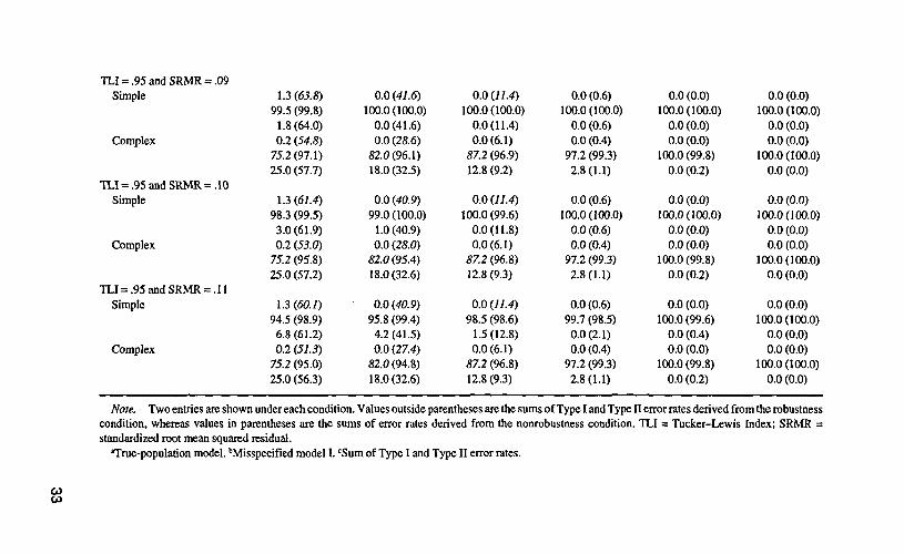
LI = .95 and SRMR =Simple

Complex

TLI = .95 and SRMR =Simple

Complex

TLI = .95 and SRMR =Simple

Complex

1.3 (63.8)99.5 (99.8)

1.8(64.0)0.2 (54.8)

75.2 (97.1)25.0 (57.7)

1.3 (61.4)98.3 (99.5)3.0 (61.9)0.2 (53.0)

75.2 (95.8)25.0 (57.2)

1.3(60.1)94.5 (98.9)6.8 (61.2)0.2 (51.3)

75.2 (95.0)25.0 (56.3)

0.0 (41.6)100.0 (100.0)

0.0(41.6)0.0 (28.6)

82.0(96.1)18.0(32.5)

0.0(40.9)99.0(100.0)

1.0(40.9)0.0 (28.0)

82.0(95.4)18.0(32.6)

0.0 (40.9)95.8 (99.4)4.2 (41.5)0.0(27.4)

82.0(94.8)18.0(32.6)

0.0 (11.4)100.0(100.0)

0.0(11.4)0.0(6.1)

87.2 (96.9)12.8 (9.2)

0.0 (11.4)100.0 (99.6)

0.0(11.8)0.0(6.1)

87.2 (96.8)12.8 (9.3)

0.0 (11.4)98.5 (98.6)

1.5(12.8)0.0(6.1)

87.2 (96.8)12.8 (9.3)

0.0 (0.6)100.0 (100.0)

0.0 (0.6)0.0 (0.4)

97.2 (99.3)2.8(1.1)

0.0 (0.6)100.0(100.0)

0.0(0.6)0.0(0.4)

97.2 (99.3)2.8(1.1)

0.0 (0.6)99.7 (98.5)

0.0(2.1)0.0 (0.4)

97.2 (99.3)2.8(1.1)

0.0 (0.0)100.0 (100.0)

0.0 (0.0)0.0 (0.0)

100.0 (99.8)0.0 (0.2)

0.0 (0.0)100.0(100.0)

0.0(0.0)0.0(0.0)

100.0(99.8)0.0 (0.2)

0.0 (0.0)100.0 (99.6)

0.0 (0.4)0.0 (0.0)

100.0 (99.8)0.0 (0.2)

0.0 (0.0)100.0 (100.0)

0.0 (0.0)0.0 (0.0)

100.0 (100.0)0.0 (0.0)

0.0(0.0)100.0(100.0)

0.0(0.0)0.0 (0.0)

100.0(100.0)0.0 (0.0)

0.0 (0.0)100.0(100.0)

0.0 (0.0)0.0 (0.0)

100.0(100.0)0.0 (0.0)

Note. Two entries are shown under each condition. Values outside parentheses are the sums of Type I and Type II error rates derived from the robustnesscondition, whereas values in parentheses are the sums of error rates derived from the nonrobustness condition. TLI = Tucker-Lewis Index; SRMR =standardized root mean squared residual.

"True-population model. bMisspecified model 1. cSum of Type I and Type II error rates.

CO4

APPENDIX TABLE 2Rejection Rates (%) and the Sum of Type I and Type II Error Rates (%) for Simple and Complex True-Population Models and Misspecified

Models (I) Based on Combinational Rules With TLI < .96 and SRMR > .06 (.07, .08, .09, .10, .11)

Cutoff Value

TLI = .96 and SRMR =.06Simple

Complex

TLI = .96 and SRMR = .07Simple

Complex

TLI = .96 and SRMR =.08Simple

Complex

150

4.2'(89.1)100.0" (100.0)

4.2C(89.1)1.2 (SO. 1)

96.0(100.0)5.2(80.1)

3.3 (82.9)100.0(100.0)

3.3 (82.9)1.2(75.0)

90.7(100.0)10.5 (75.0)

3.3 (77.0)100.0 (100.0)

3.3 (77.0)1.2(69.5)

89.5 (99.5)11.7(69.8)

250

0.0 (65.8)100.0(100.0)

0.0 (65.8)0.0(55.8)

95.3 (100.0)4.7 (53.8)

0.0 (60.9)100.0(100.0)

0.0 (60.9)0.0 (49.4)

95.2 (99.6)4.8 (49.8)

0.0 (57.6)100.0(100.0)

0.0 (57.6)0.0 (46.4)

95.2 (99.1)4.8 (47.3)

500

0.0 (20.8)100.0(100.0)

0.0 (20.8)0.0 (12.9)

99.0(99.9)0.0(13.0)

0.0 (20.3)100.0(100.0)

0.0 (20.3)0.0 (11.5)

99.0 (99.9)1.0(11.6)

0.0 (20.0)100.0 (100.0)

0.0 (20.0)

0.0 a/J)99.0 (99.6)

1.0(11.7)

N

1,000

0.0 (2.6)100.0 (100.0)

0.0 (2.6)0.0(1.1)

100.0(100.0)0.0(1.1)

0.0 (2.6)100.0(100.0)

0.0 (2.6)0.0(0.8)

100.0 (100.0)0.0 (0.8)

0.0 (2.6)100.0 (100.0)

0.0 (2.6)0.0 (0.8)

100.0 (100.0)0.0 (0.8)

2,500

0.0(0.4)100.0 (100.0)

0.0 (0.4)0.0(0.0)

100.0(100.0)0.0 (0.0)

0.0 (0.4)100.0 (100.0)

0.0 (0.4)0.0 (0.0)

100.0 (100.0)0.0 (0.0)

0.0 (0.4)100.0 (100.0)

0.0 (0.4)0.0(0.0)

100.0 (100.0)0.0 (0.0)

5,000

0.0 (0.0)100.0(100.0)

0.0 (0.0)0.0 (0.0)

100.0 (100.0)0.0 (0.0)

0.0 (0.0)100.0 (100.0)

0.0 (0.0)0.0 (0.0)

100.0 (100.0)0.0 (0.0)

0.0 (0.0)100.0(100.0)

0.0 (0.0)0.0 (0.0)

100.0(100.0)0.0 (0.0)

LI = .96andSRMR = .CSimple

Complex

TLI = .96andSRMR = .lSimple

Complex

TLI = .96andSRMR = .lSimple

Complex

3.3 (73.1)99.5 (99.8)

3.8 (73.3)1.2(65.4)

£9.5(98.5)11.7(66.9)

3.3 (70.8)98.5 (99.8)4.8(71.0)1.2(63.6)

59.5(98.1)11.7(65.5)

3.3 (69.5)95.3 (99.3)

8.0 (70.2)1.2 (61.9)

89.5 (98.0)11.7(63.9)

0.0 (56.6)100.0 (100.0)

0.0 (56.6)0.0 (44.9)

95.2 (98.9)4.8 (46.0)

0.0 (55.9)99.0 (100.0)

1.0(55.9)0.0 (44.3)

95.2 (98.9)4.8 (45.4)

0.0 (55.9)95.8 (99.6)4.2 (56.3)0.0 (43.6)

95.2 (98.6)4.8 (45.0)

0.0 (79.9)100.0 (100.0)

0.0 (19.9)0.0 (11.0)

99.0 (99.6)1.0(11.4)

0.0 (19.9)100.0(100.0)

0.0(19.9)0.0 (11.0)

99.0 (99.6)1.0(11.4)

0.0 (19.9)98.8 (99.5)

1.2(20.4)1.0 (11.0)

99.0 (99.6)1.0(11.4)

0.0 (2.6)100.0 (100.0)

0.0 (2.6)0.0 (0.8)

100.0 (100.0)0.0 (0.8)

0.0 (2.6)100.0 (100.0)

0.0(2.6)0.0 (0.8)

100.0(100.0)0.0 (0.8)

0.0(2.6)99.7 (98.8)0.3 (3.8)0.0 (0.8)

100.0 (100.0)0.0 (0.8)

0.0(0.4)100.0 (100.0)

0.0(0.4)0.0(0.0)

100.0(100.0)0.0 (0.0)

0.0 (0.4)100.0(100.0)

0.0(0.4)0.0 (0.0)

100.0 (100.0)0.0 (0.0)

0.0(0.4)100.0(99.6)

0.0(0.8)0.0 (0.0)

100.0 (100.0)0.0 (0.0)

0.0 (0.0)100.0(100.0)

0.0 (0.0)0.0(0.0)

100.0 (100.0)0.0 (0.0)

0.0 (0.0)100.0 (100.0)

0.0 (0.0)0.0 (0.0)

100.0 (100.0)0.0 (0.0)

0.0 (0.0)100.0 (100.0)

0.0 (0.0)0.0 (0.0)

100.0 (100.0)0.0 (0.0)

Note. Two entries are shown under each condition. Values outside parentheses are the sums of Type I and Type II error rates derived from the robustnesscondition, whereas values in parentheses are the sums of error rates derived from the nonrobustness condition. TLI = Tucker-Lewis Index; SRMR =standardized root mean squared residual.

'True-population model. bMisspecified model I. cSum of Type I and Type II error rates.

CO

en

APPENDIX TABLE 3Rejection Rates (%) and the Sum of Type I and Type II Error Rates (%) for Simple and Complex True-Population Models and Misspecified

Models (I) Based on Combinational Rules With BL89 < .95 and SRMR > .06 (.07, .08, .09, .10, .11)

Cutoff Value

BL89 = .95 and SRMR = .06Simple

Complex

BL89 = .95 and SRMR = .07Simple

Complex

BL89 = .95 and SRMR = .08Simple

Complex

ISO

1.7* (78.1)100.0b (100.0)

1.7C (78.1)0.0 (60.6)

94.0 (99.6)6.0(61.0)

0.2 (65.3)100.0(100.0)

0.2 (65.3)

0.0(50.-064.8 (99.3)35.2(51.1)

0.2 (58.6)100.0 (100.0)

0.2 (65.3)0.0 (43.8)

57.5(97.9)48.5 (45.9)

250

0.0 (38.8)100.0(100.0)

0.0 (38.9)0.0 (26.3)

83.8 (98.6)16.2 (27.7)

0.0 (33.4)100.0(100.0)

0.0 (33.4)0.0(27.8)

50.3 (97.4)49.7 (24.4)

0.0(30.7)100.0(99.9)

0.0 (30.2)0.0(78.5)

47.5(93.0)52.2 (25.8)

N

500

0.0 (7.6)100.0(100.0)

0.0 (7.6)0.0 (6.6)

67.5 (96.5)32.5(10.1)

0.0 (6.8)100.0(100.0)

0.0 (6.8)0.0 (5.0)

43.3 (94.0)56.7(11.0)

0.0 (6.5)100.0 (100.0)

0.0 (6.5)0.0 (4.6)

43.2 (88.3)56.8 (0.0)

1,000

0.0 (0.4)100.0(100.0)

0.0 (0.4)0.0 (0.8)

54.7(97.9)45.3 (8.9)

0.0 (0.4)100.0(100.0)

0.0 (0.4)0.0(0.4)

41.7(87.4)58.3 (13.0)

0.0 (0.4)100.0 (100.0)

0.0(0.4)0.0 (0.4)

41.7(82.9)58.3 (17.5)

2,500

0.0 (0.0)100.0 (100.0)

0.0 (0.0)0.0 (0.0)

36.5(80.9)63.5(19.1)

0.0 (0.0)100.0(100.0)

0.0 (0.0)0.0 (0.0)

33.0(72.8)77.0 (27.2)

0.0 (0.0)100.0(100.0)

0.0(0.0)0.0 (0.0)

33.0(70.9)77.0(29.1)

5,000

0.0 (0.0)100.0 (100.0)

0.0 (0.0)0.0 (0.0)

29.3 (73.8)70.7 (26.2)

0.0 (0.0)100.0 (100.0)

0.0 (0.0)0.0 (0.0)

28.2 (66.8)71.8(33.2)

0.0 (0.0)100.0 (100.0)

0.0 (0.0)0.0 (0.0)

28.2 (65.5)71.8 (34.5)

BL89 = .95 and SRMR = .09Simple

Complex

BL89 = .95andSRMR = .10Simple

Complex

BL89 = .95andSRMR = . l lSimple

Complex

0.2 {54.6)99.5 (99.8)0.7 (54.8)0.0 (39.9)

49.8(94.3)50.2 (45.6)

0.2 (52.5)99.5 (99.8)

1.9 (52.9)0.0 (38.1)

49.8(943)50.2 (45.6)

0.2 (51.0)94.3 (98.8)

5.9 (52.2)0.0 (36.4)

49.8(90.8)50.2 (45.6)

0.0 (30.1)100.0(99.9)

0.0(29.2)0.0 (17.3)

47.8(90.8)52.2 (26.5)

0.0 (28.4)100.0(99.9)

1.1 (28.9)0.0(16.6)

47.8(89.1)52.2 (27.5)

0.0(28.4)95.7(98.1)4.3 (30.3)0.0 (MO)

47.8(88.4)57.2 (27.6)

0.0(6.5)100.0(100.0)

0.0(6.4)0.0(4.4)

43.2 (86.5)56.8(17.9)

0.0(6.4)100.0(100.0)

0.0(7.0)0.0(4.4)

43.2(85.9)56.8 (18.5)

0.0(6.4)98.5 (97.3)

1.5(9.1)0.0(4.4)

43.2 (85.6)56.8 (18.8)

0.0 (0.4)100.0(100.0)

0.0(0.4)0.0 (0.4)

41.7(82.4)58.3 (18.0)

0.0 (0.4)100.0(100.0)

0.0(0.4)0.0(0.4)

41.7(82.4)58.3 (18.0)

0.0(0.4)99.7 (98.5)0.3 (0.0)0.0(0.4)

41.7(82.4)58.3 (18.0)

0.0(0.0)100.0(100.0)

0.0(0.0)0.0(0.0)

33.0(70.9)77.0(29.2)

0.0 (0.0)100.0(100.0)

0.0(0.0)0.0 (0.0)

33.0(70.8)77.0 (29.2)

0.0 (0.0)100.0(99.6)

0.0 (0.4)0.0 (0.0)

33.0(70.8)77.0 (29.2)

0.0(0.0)100.0(100.0)

0.0(0.0)0.0 (0.0)

28.2 (65.5)71.8 (34.5)

0.0 (0.0)100.0(100.0)

0.0 (0.0)0.0 (0.0)

28.2 (65.5)71.8 (34.5)

0.0 (0.0)100.0(100.0)

0.0 (0.0)0.0 (0.0)

28.2 (65.5)71.8 (34.5)

Note. Two entries are shown under each condition. Values outside parentheses are the sums of Type I and Type II error rates derived from the robustnesscondition, whereas values in parentheses are the sums of error rates derived from the nonrobustness condition. BL89 = Bollen's Fit Index (1989); SRMR =standardized root mean squared residual.

"True-population model. 'Misspecified model I. cSum of Type I and Type II error rates.

COJ

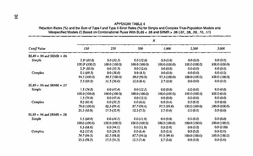
COCO

APPENDIX TABLE 4Rejection Rates (%) and the Sum of Type I and Type II Error Rates (%) for Simple and Complex True-Population Models and

Misspecified Models (I) Based on Combinational Rules With BL89 < .96 and SRMR > .06 (.07, .08, .09, .10, .11)

Cutoff Value

BL89 = .96 and SRMR = .06Simple

Complex

BL89 = .96 and SRMR = .07Simple

Complex

BL89 = .96 and SRMR = .08Simple

Complex

150

2.5" (83.8)100.0" (100.0)

2.5° (83.8)0.2 (69.5)

94.7 (100.0)5.5 (69.5)

1.5 (74.8)100.0(100.0)

1.5(74.8)0.2 (63.8)

79.0(100.0)21.2 (63.8)

1.5 (68.8)100.0(100.0)

1.5 (68.8)0.2 (57.8)

74.7(993)25.3 (58.5)

250

0.0 (52.3)100.0(100.0)

0.0 (52.3)0.0 (36.6)

88.5 (100.0)11.5(36.6)

0.0 (47.4)100.0(100.0)

0.0 (47.4)0.0 (32.3)

82.5(99.4)17.5 (32.9)

0.0(44.1)100.0(100.0)

0.0(44.1)0.0(29.5)

82.5 (98.0)17.5(31.3)

500

0.0(12.6)100.0(100.0)

0.0(12.6)0.0 (8.3)

88.0(99.9)12.0 (8.4)

0.0(72.7)100.0(100.0)

0.0(12.1)0.0 (6.6)

87.7 (99.4)12.3 (7.2)

0.0(77.9)100.0(100.0)

0.0(11.9)0.0 (6.4)

87.7 (99.0)12.3 (7.4)

N

1,000

0.0(0.8)100.0(100.0)

0.0 (0.8)0.0 (0.8)

97.3 (100.0)2.7 (0.8)

0.0(0.8)100.0(100.0)

0.0(0.8)0.0(0.4)

97.3 (99.8)2.7 (0.6)

0.0(0.8)100.0(100.0)

0.0 (0.8)0.0 (0.4)

97.3 (99.8)2.7 (0.6)

2,500

0.0 (0.0)100.0(100.0)

0.0 (0.0)0.0(0.0)

100.0 (100.0)0.0 (0.0)

0.0 (0.0)100.0(100.0)

0.0 (0.0)0.0 (0.0)

100.0(100.0)0.0(0.0)

0.0(0.0)100.0(100.0)

0.0(0.0)0.0(0.0)

100.0(100.0)0.0 (0.0)

5,000

0.0 (0.0)100.0(100.0)

0.0 (0.0)0.0 (0.0)

100.0(100.0)0.0(0.0)

0.0 (0.0)100.0 (0.0)

0.0 (0.0)0.0 (0.0)

100.0(100.0)0.0 (0.0)

0.0 (0.0)100.0(100.0)

0.0 (0.00)0.0 (0.0)

100.0(100.0)0.0 (0.0)

BL89 = .96 and SRMR = .09Simple

Complex

BL89 = .96andSRMR = .10Simple

Complex

BL89 = .96 and SRMR = .11Simple

Complex

1.5 (64.9)99.5 (99.8)2.0(65.1)0.2 (53.9)

74.5(97.5)25.7 (56.4)

1.5 (62.5)98.3 (99.5)

3.2 (63.0)0.2 (52.1)

74.5(96.6)25.7 (55.5)

1.5 (61.3)94.8 (99.0)6.7 (62.3)0.2 (50.4)

74.5 (95.9)25.7 (54.5)

0.0(43./)100.0(100.0)

0.0(43.1)0.0(27.5)

52.5(97.4)17.5 (30.4)

0.0 (42.4)99.0 (100.0)

1.0(42.4)0.0(27./)

82.5 (97.3)17.5 (29.8)

0.0 (42.4)95.8(99.4)4.2 (43.0)0.0 (26.5)

82.5 (96.9)17.5 (29.6)

0.0 (11.8)100.0(100.0)

0.0(11.8)0.0(6.1)

87.7(98.8)12.3 (7.3)

0.0 (11.8)100.0 (99.6)

0.0 (12.2)0.0(6.1)

57.7(98.8)12.3 (7.3)

0.0 (11.8)98.5 (98.6)

1.5(13.2)0.0(6.1)

87.7(98.8)12.3 (7.3)

0.0(0.8)100.0(100.0)

0.0 (0.8)0.0 (0.4)

97.3 (99.8)2.7 (0.6)

0.0 (0.8)100.0 (100.0)

0.0 (0.8)0.0 (0.4)

97.3 (99.8)2.7 (0.6)

0.0 (0.0)99.7 (98.5)0.3 (1.5)0.0 (0.0)

100.0 (99.8)0.0(0.2)

0.0(0.0)100.0(100.0)

0.0(0.0)0.0 (0.0)

100.0 (100.0)0.0 (0.0)

0.0(0.0)100.0(100.0)

0.0(0.0)0.0(0.0)

100.0(100.0)0.0 (0.0)

0.0 (0.0)100.0 (99.6)

0.0 (0.4)0.0(0.0)

100.0(100.0)0.0(0.0)

0.0(0.0)100.0(100.0)

0.0 (0.0)0.0 (0.0)

100.0 (100.0)0.0(0.0)

0.0(0.0)100.0(100.0)

0.0(0.0)0.0(0.0)

100.0(100.0)0.0(0.0)

0.0 (0.0)100.0(100.0)

0.0 (0.0)0.0 (0.0)

100.0(100.0)0.0(0.0)

Note. Two entries are shown under each condition. Values outside parentheses are the sums of Type I and Type II error rates derived from the robustnesscondition, whereas values in parentheses are the sums of error rates derived from the nonrobustness condition. BL89 = Bollen' s Fit Index (1989); SRMR =standardized root mean squared residual.

'True-population model. bMisspecified model I. cSum of Type I and Type II error rates.

COCO

APPENDIX TABLE 5Rejection Rates (%) and the Sum of Type I and Type II Error Rates (%) for Simple and Complex True-Population Models and

Misspecified Models (I) Based on Combinational Rules With RNI (or CFI) < .95 and SRMR > .06 (.07, .08, .09, .10, .11)

Cutoff Value

RNI (or CH) = .95 and SRMR = .06Simple

Complex

RNI (or CFI) = .95 and SRMR = .07Simple

Complex

RNI (or CFI) = .95 and SRMR = .08Simple

Complex

150

1.7' (78.5)100.0" (100.0)

1.7C(78.5)0.0 (61.1)

94.0 (99.6)0.6(61.5)

0.2 {66.3)100.0 (100.0)

0.2 (66.3)0.0 (57.0)

65.5 (99.3)34.5(51.7)

0.2 (59.6)100.0(100.0)

0.2 (59.6)0.0(44.4)

53.0(91.9)47.0 (46.5)

250

0.0 (39.6)100.0(100.0)

0.0 (39.6)0.0 (26.6)

83.8 (9Z.Z)16.2 (27.8)

0.0 (34.3)100.0(100.0)

0.0 (34.3)0.0 (22.1)

51.3 (97.5)48.7 (24.6)

0.0 (31.0)100.0(100.0)

0.0(31.0)0.0 (19.1)

49.3 (93.3)50.8 (25.8)

500

0.0(7.6)100.0 (100.0)

0.0 (7.6)0.0(6.6)

67.7(96.9)32.3 (9.7)

0.0(6.8)100.0(100.0)

0.0(6.8)0.0 (5.0)

44.2 (94.4)55.8 (10.6)

0.0(6.5)100.0(100.0)

0.0(6.5)0.0 (4.6)

44.0(88.9)56.0(15.7)

N

1,000

0.0 (0.4)100.0 (100.0)

0.0 (0.0)0.0(0.8)

55.0(92.1)45.0 (8.7)

0.0 (0.4)100.0(100.0)

0.0 (0.4)0.0(0.4)

42.3 (87.8)57.7 (12.6)

0.0 (0.4)100.0(100.0)

0.0 (0.4)0.0 (0.4)

42.3 (83.3)57.7 (17.1)

2,500

0.0 (0.0)100.0(100.0)

0.0 (0.0)0.0 (0.0)

36.7(81.0)63.3 (19.0)

0.0 (0.0)100.0(100.0)

0.0 (0.0)0.0 (0.0)

33.3 (73.0)66.7 (27.0)

0.0 (0.0)100.0(100.0)

0.0 (0.0)0.0 (0.0)

33.3(71.1)66.7 (28.9)

5,000

0.0 (0.0)100.0(100.0)

0.0(0.0)0.0(0.0)

29.5(74.1)70.5 (25.9)

0.0(0.0)100.0 (100.0)

0.0(0.0)0.0(0.0)

28.3 (67.0)71.7 (23.0)

0.0 (0.0)100.0(100.0)

0.0(0.0)0.0 (0.0)

28.3 (65.9)71.7(34.1)

RNI (or CFI) = .95 and SRMR = .09Simple

Complex

RNI (or CFI) = .95 and SRMR = .10Simple

Complex

RNI (or CFI) = .95 and SRMR = .11Simple

Complex

0.2 (54.6)99.5 (99.8)

0.7 (54.8)0.0 (39.9)

49.8(943)50.2 (45.6)

0.2 (53.3)98.3 (99.4)

1.9(0.0)0.0 (38.8)

51.5(92.5)48.5 (46.3)

0.2 (52.0)94.3 (98.8)

5.9 (53.2)0.0 (37.0)

51.5(91.3)48.5 (45.7)

0.0(29./)100.0(99.9)

0.0 (29.2)0.0 (17.3)

47.8(90.8)52.2 (26.5)

0.0 (29.3)99.0 (99.6)

1.0(29.7)0.0 (17.0)

49.2 (89.5)50.8 (27.5)

0.0 (29.3)95.7 (98.3)4.3 (31.0)0.0(16.4)

49.2 (88.8)50.8 (27.6)

0.0(6.4)100.0(100.0)

0.0(6.4)0.0(4.4)

43.2(86.5)56.8(17.9)

0.0(6.4)100.0(99.4)

0.0(7.0)0.0(4.4)

44.0(86.6)56.0(17.8)

0.0(6.4)98.5 (97.3)

1.5(9.1)0.0(4.4)

44.0(86.4)56.0(17.8)

0.0(0.4)100.0(100.0)

0.0 (0.4)0.0 (0.4)

41.7(82.4)58.3 (18.0)

0.0 (0.4)100.0(100.0)

0.0 (0.4)0.0 (0.4)

42.3 (82.8)57.7 (17.6)

0.0 (0.4)99.7 (98.5)

0.3 (1.9)0.0 (0.4)

42.3 (82.8)57.7 (17.6)

0.0(0.0)100.0(100.0)

0.0 (0.0)0.0 (0.0)

33.0(70.8)67.0 (29.2)

0.0 (0.0)100.0(100.0)

0.0(0.0)0.0(0.0)

33.3(71.0)66.7 (29.0)

0.0 (0.0)100.0(99.6)

0.0 (0.4)0.0 (0.0)

33.3 (71.0)66.7 (29.0)

0.0 (0.0)100.0(100.0)

0.0 (0.0)0.0 (0.0)

2S.2 (65.5)71.8 (34.5)

0.0 (0.0)100.0 (100.0)

0.0 (0.0)0.0 (0.0)

28.3 (65.9)71.7(34.1)

0.0 (0.0)100.0 (100.0)

0.0 (0.0)0.0 (0.0)

28.3 (65.9)71.7(34.1)

Note. Two entries are shown under each condition. Values outside parentheses are the sums of Type I and Type II error rates derived from the robustnesscondition, whereas values in parentheses are the sums of error rates derived from the nonrobustness condition. RNI = Relative Noncentrality Index; CFI =Comparative Fit Index; SRMR = standardized root mean squared residual.

•True-population model. bMisspecified model I. cSum of Type I and Type II error rates.

APPENDIX TABLE 6Rejection Rates (%) and the Sum of Type I and Type II Error Rates (%) for Simple and Complex True-Population Models and

Misspecified Models (I) Based on Combinational Rules With RNI (or CFI) < .96 and SRMR > .06 (.07, .08, .09, .10, .11)

Cutoff Value

RNI (or CFI) = .96 and SRMR = .06Simple

Complex

RNI (or CFI) = .96 and SRMR = .07Simple

Complex

RNI (or CFI) = .96 and SRMR = . 08Simple

Complex

150

2.5' {84.3)100.0" (100.0)

2.5= (84.3)0.2 (70.3)

94.7 (100.0)5.5 (70.3)

1.5 (75.6)100.0(100.0)

1.5(75.6)0.2 (64.6)

80.3 (100.0)19.9 (64.6)

1.5(69.6)100.0(100.0)

1.5(69.6)0.2 (58.6)

76.5(98.0)23.7 (59.3)

250

0.0 (52.9)100.0(100.0)

0.0 (52.9)0.0 (37.5)

88.7(100.0)11.3(37.5)

0.0 (48.0)100.0(100.0)

0.0(48.0)0.0 (33.1)

83.2 (99.4)16.8 (33.7)

0.0 (44.8)100.0 (100.0)

0.0 (44.8)0.0 (30.1)

83.2 (99.4)16.8 (32.1)

500

0.0 (13.0)100.0(100.0)

0.0 (13.0)0.0 (8.3)

88.5 (99.9)11.5(8.4)

0.0 (12.5)100.0 (100.0)

0.0 (12.5)0.0 (6.6)

88.2 (99.4)11.8(7.2)

0.0 (12.3)100.0 (100.0)

0.0 (12.3)0.0 (6.4)

88.2 (99.4)11.8(7.4)

N

1,000

0.0 (0.9)100.0 (100.0)

0.0 (0.9)0.0 (0.8)

97.3 (100.0)2.7 (0.8)

0.0 (0.9)100.0(100.0)

0.0 (0.9)0.0 (0.4)

97.3 (99.9)2.7 (0.5)

0.0 (0.9)100.0(100.0)

0.0 (0.9)0.0 (0.4)

97.3 (99.9)2.7 (0.5)

2,500

0.0(0.0)100.0(100.0)

0.0 (0.0)0.0 (0.0)

100.0(100.0)0.0(0.0)

0.0 (0.0)100.0(100.0)

0.0 (0.0)0.0 (0.0)

100.0(100.0)0.0(0.0)

0.0 (0.0)100.0(100.0)

0.0 (0.0)0.0 (0.0)

100.0(100.0)0.0 (0.0)

5,000

0.0 (0.0)100.0(100.0)

0.0 (0.0)0.0(0.0)

100.0 (100.0)0.0 (0.0)

0.0 (0.0)100.0(100.0)

0.0 (0.0)0.0 (0.0)

100.0(100.0)0.0 (0.0)

0.0 (0.0)100.0(100.0)

0.0 (0.0)0.0 (0.0)

100.0(100.0)0.0(0.0)

RNI (or CFI) = .96 and SRMR = .09Simple

Complex

RNI (or CFI) = .96 and SRMR = .10Simple

Complex

RNI (or CFI) = .96 and SRMR = .11Simple

Complex

1.5 (65.8)99.5 (99.8)2.0(66.0)0.2 (54.8)

76.3(97.6)23.9 (57.2)

\.5 (63.4)98.3 (99.5)

3.2 (63.9)0.2 (53.0)

76.3 (96.9)23.9 (56.1)

1.5 (62.7)94.8 (99.0)

6.7 (63.1)0.2 (51.3)

76.3 (96.3)23.9 (55.0)

0.0 (43.8)100.0(100.0)

0.0 (43.8)0.0 (28.6)

83.2 (97.4)16.8(31.2)

0.0 (43.0)99.0(100.0)

1.0(0.0)0.0 (28.0)

83.2 (97.3)16.8 (30.7)

0.0 (45.0)95.8 (99.4)

4.2 (43.6)0.0 (27.4)

83.2 (96.9)16.8(30.5)

0.0(72.7)100.0(100.0)

0.0(12.1)0.0(6.1)

88.2 (98.8)11.8(7.3)

0.0(72.7)100.0(99.6)

0.0(12.5)0.0(6.1)

88.2 (98.8)11.8(7.3)

0.0(72.7)98.5 (98.8)

1.5 (13.3)0.0 (6.1)

88.2 (98.8)11.8(7.3)

0.0 (0.9)100.0 (100.0)

0.0 (0.9)0.0 (0.4)

97.3 (99.9)2.7 (0.5)

0.0 (0.9)100.0(100.0)

0.0(0.9)0.0(0.4)

97.3 (99.9)2.7 (0.5)

0.0(0.9)99.7 (98.5)

0.3 (2.4)0.0 (0.4)

97.3 (99.9)2.7 (0.5)

0.0 (0.0)100.0 (100.0)

0.0 (0.0)0.0 (0.0)

100.0 (100.0)0.0 (0.0)

0.0 (0.0)100.0(100.0)

0.0 (0.0)0.0 (0.0)

100.0(100.0)0.0 (0.0)

0.0 (0.0)100.0 (99.6)

0.0 (0.0)0.0 (0.0)

100.0(100.0)0.0 (0.0)

0.0 (0.0)100.0(100.0)

0.0 (0.0)0.0 (0.0)

100.0(100.0)0.0 (0.0)

0.0 (0.0)100.0(100.0)

0.0 (0.0)0.0 (0.0)

100.0(100.0)0.0 (0.0)

0.0(0.0)100.0(100.0)

0.0 (0.0)0.0 (0.0)

100.0(100.0)0.0 (0.0)

Note. Two entries are shown under each condition. Values outside parentheses are the sums of Type I and Type II error rates derived from the robustnesscondition, whereas values in parentheses are the sums of error rates derived from the nonrobustness condition. RNI = Relative Noncentrality Index; CFI =Comparative Fit Index; SRMR = standardized root mean squared residual.

•True-population model. bMisspecified model I. cSum of Type I and Type II error rates.

APPENDIX TABLE 7Rejection Rates (%) and the Sum of Type I and Type II Error Rates (%) for Simple and Complex True-Population Models and

Misspecified Models (I) Based on Combinational Rules With Gamma Hat < .95 and SRMR > .06 (.07, .08, .09, .10, .11)

Cutoff Value

Gamma Hat = .95 and SRMR = .06Simple

Complex

Gamma Hat = .95 and SRMR = .07Simple

Complex

Gamma Hat = .95 and SRMR = .08Simple

Complex

150

1.5" (78.3)100.0" (100.0)

1.5C(78.3)0.0(67.5)

94.3 (99.9)5.7 (32.8)

0.0 (65.0)100.0(100.0)

0.0 (65.0)0.0(60.7)

71.5 (99.9)28.5 (60.2)

0.0 (58.0)100.0 (100.0)

0.0 (58.0)0.0(53.8)

67.2 (98.9)37.3(54.1)

250

0.0 (35.9)100.0(100.0)

0.0(35.9)0.0(32.0)

85.5 (100.0)14.5 (32.0)

0.0 (30.4)100.0(100.0)

0.0 (30.4)0.0 (27.4)

63.0 (98.9)37.0(28.5)

0.0(27.7)100.0(99.6)

0.0(27.5)0.0 (24.4)

61.2 (95.1)38.8(29.3)

500

0.0(7.3)100.0 (100.0)

0.0 (7.3)0.0 (7.8)

73.0 (99.3)27.0(8.5)

0.0 (6.4)100.0(100.0)

0.0(6.4)0.0(6.1)

60.7(97.1)39.3 (9.0)

0.0(6.1)100.0 (100.0)

0.0(6.1)0.0(5.9)

60.7(93.5)39.3 (0.0)

N

1,000

0.0(0.4)100.0(100.0)

0.0 (0.4)0.0 (0.8)

69.8 (96.6)30.2 (4.2)

0.0 (0.4)100.0(100.0)

0.0 (0.4)0.0(0.4)

65.5(93.0)34.2 (7.4)

0.0 (0.4)100.0 (100.0)

0.0 (0.4)0.0 (0.4)

65.8(91.9)34.2 (8.5)

2,500

0.0 (0.0)100.0(100.0)

0.0 (0.0)0.0 (0.0)

68.2 (94.3)31.8 (5.7)

0.0 (0.0)100.0(100.0)

0.0(0.0)0.0(0.0)

68.2(90.9)31.8(9.1)

0.0(0.0)100.0(100.0)

0.0(0.0)0.0 (0.0)

68.2(90.9)31.8(9.1)

5,000

0.0 (0.0)100.0(100.0)

0.0 (0.0)0.0 (0.0)

78.3 (100.0)21.7(0.0)

0.0 (0.0)100.0(100.0)

0.0 (0.0)0.0 (0.0)

78.3 (91.9)21.7(8.1)

0.0(0.0)100.0 (100.0)

0.0 (0.0)0.0 (0.0)

78.3 (91.9)21.7(8.1)

Gamma Hat = .95 and SRMR = .09Simple

Complex

Gamma Hat = .95 and SRMR = .10Simple

Complex

Gamma Hat = .95 and SRMR = .11Simple

Complex

0.0 (53.9)99.5 (99.6)0.0 (54.3)0.0 (49.9)

61.8 (96.0)38.2 (53.9)

0.0 (51.4)98.3 (99.3)

1.7(52.1)0.0(48.7)

61.8 (94.5)38.2 (53.6)

0.0 (50.1)94.3 (98.5)

5.7 (51.6)0.0 (46.4)

61.8(933)38.2(53.1)

0.0 (26.7)100.0(99.4)

0.0 (26.7)0.0 (76.0)

61.2 (93.3)38.8 (82.7)

0.0 (25.4)99.0 (99.0)

1.0(26.4)0.0 (22J)

67.2 (92.7)38.8 (30.2)

0.0 (25.4)95.7 (97.3)4.3 (28.1)0.0 (27.6)

67.2 (91.5)38.8 (30.1)

0.0(6.0)100.0(100.0)

0.0 (6.0)0.0 (5.6)

60.7(92.8)39.3 (12.8)

0.0 (6.0)100.0 (99.4)

0.0(6.6)0.0 (5.6)

60.7(92.6)39.3 (13.0)

0.0 (6.0)98.5 (96.9)

1.5(6.6)0.0 (5.6)

60.7(92.5)39.3 (13.0)

0.0(0.4)100.0(100.0)

0.0 (0.4)0.0 (0.4)

65.8(97.7)34.2 (8.5)

0.0 (0.4)100.0 (100.0)

0.0(0.4)0.0(0.4)

65.8(97.7)34.2 (8.5)

0.0 (0.4)99.7 (98.4)0.3 (2.0)0.0 (0.4)

65.8(97.7)34.2 (8.5)

0.0 (0.0)100.0 (100.0)

0.0 (0.0)0.0 (0.0)

68.2 (90.9)31.8 (9.1)

0.0 (0.0)100.0 (100.0)

0.0 (0.0)0.0 (0.0)

68.2 (90.9)31.8(9.1)

0.0 (0.0)100.0 (99.6)

0.0 (0.4)0.0 (0.0)

68.2 (90.9)31.8(9.1)

0.0 (0.0)100.0 (100.0)

0.0 (0.0)0.0 (0.0)

78.3 (91.9)21.7(8.1)

0.0 (0.0)100.0 (100.0)

0.0 (0.0)0.0

78.3 (91.9)21.7(8.1)

0.0 (0.0)100.0(100.0)

0.0 (0.0)0.0 (0.0)

78.3 (91.9)21.7(8.1)

Note. Two entries are shown under each condition. Values outside parentheses are the sums of Type I and Type II error rates derived from the robustnesscondition, whereas values in parentheses are the sums of error rates derived from the nonrobustness condition. SRMR = standardized root mean squaredresidual.

•True-population model. bMisspecified model I. cSum of Type I and Type II error rates.

APPENDIX TABLE 8Rejection Rates (%) and the Sum of Type I and Type II Error Rates (%) for Simple and Complex True-Population Models and

Misspecified Models (I) Based on Combinational Rules With Gamma Hat < .96 and SRMR > .06 (.07, .08, .09, .10, .11)

Cutoff Value

Gamma Hat = .96 and SRMR = .06Simple

Complex

Gamma Hat = .96 and SRMR = .07Simple

Complex

Gamma Hat = .96 and SRMR = .08Simple

Complex

150

2.2' (84.1)100.0" (100.0)

2.2'(84.1)0.3 (78.3)

95.0 (100.0)5.3 (78.3)

1.0 (75.1)100.0(100.0)

1.0(75.1)0.3 (73.0)

83.2 (100.0)17.1 (73.0)

1.0 (68.8)100.0(100.0)

1.0(68.8)0.3 (67.3)

80.2 (99.3)20.1 (68.0)

250

0.0 (47.3)100.0(100.0)

0.0 (47.3)0.0 (46.4)

90.5 (100.0)9.5 (46.4)

0.0 (42.4)100.0(100.0)

0.0 (42.4)0.0(42.0)

88.0 (99.4)12.0(42.6)

0.0(39.7)100.0 (100.0)

0.0(39.1)0.0(39.0)

87.8 (98.4)12.2 (40.1)

500

0.0(10.4)100.0(100.0)

0.0 (10.4)0.0 (10.8)

95.5 (99.9)4.5 (10.9)

0.0(9.8)100.0(100.0)

0.0(9.8)0.0 (9.4)

95.3 (99.6)4.7 (9.8)

0.0 (9.5)100.0 (100.0)

0.0(9.5)0.0(9./)

95.3 (99.4)4.7 (9.7)

N

1,000

0.0 (0.5)100.0 (100.0)

0.0 (0.5)0.0(0.9)

99.3 (99.9)0.7(1.0)

0.0 (0.5)100.0(100.0)

0.0(0.5)0.0(0.5)

100.0(99.8)0.0 (0.7)

0.0(0.5)100.0(100.0)

0.0(0.5)0.0(0.5)

99.3 (99.8)0.7 (0.7)

2,500

0.0(0.0)100.0(100.0)

0.0(0.0)0.0(0.0)

100.0(100.0)0.0 (0.0)

0.0 (0.0)100.0(100.0)

0.0(0.0)0.0(0.0)

100.0 (100.0)0.0 (0.0)

0.0(0.0)100.0(100.0)

0.0 (0.0)0.0 (0.0)

100.0(100.0)0.0(0.0)

5,000

0.0 (0.0)100.0(100.0)

0.0 (0.0)0.0 (0.0)

100.0(100.0)0.0 (0.0)

0.0 (0.0)100.0(100.0)

0.0 (0.0)0.0 (0.0)

100.0(100.0)0.0(0.0)

0.0(0.0)100.0(100.0)

0.0 (0.0)0.0 (0.0)

100.0(100.0)0.0(0.0)

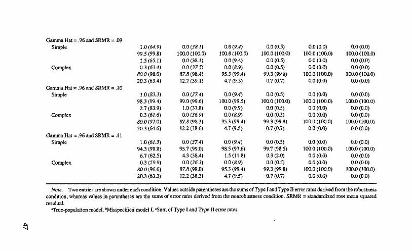
Gamma Hat = .96 and SRMR = .09Simple

Complex

Gamma Hat = .96 and SRMR = .10Simple

Complex

Gamma Hat = .96 and SRMR = .11Simple

Complex

1.0 (64.9)99.5 (99.8)

1.5(65.1)0.3 (63.4)

80.0 (98.0)20.3 (65.4)

1.0(83.3)98.3 (99.4)2.7 (83.9)0.3 (61.6)

80.0 (97.0)20.3 (64.6)

1.0(67.3)94.3 (98.8)

6.7 (62.5)0.3 (59.9)

80.0 (96.6)20.3 (63.3)

0.0 (38.1)100.0(100.0)

0.0(38.1)0.0(37.5)

87.8 (98.4)12.2(39.1)

0.0 (37.4)99.0 (99.6)

1.0(37.8)0.0 (36.9)

87.8 (98.3)12.2 (38.6)

0.0 (37.4)95.7 (99.0)

4.3 (38.4)0.0 (36.3)

87.8 (98.0)12.2 (38.3)

0.0(9.4)100.0(100.0)

0.0 (9.4)0.0 (8.9)

95.3 (99.4)4.7 (9.5)

O.O (9.4)

10O.0 (99.5)0.0 (9.9)O.O (8.9)

95.3 (99.4)4.7 (9.5)

0.0 (9.4)98.5 (97.6)

1.5(11.8)0.0 (8.9)

95.3 (99.4)4.7 (9.5)

0.0 (0.5)100.0(100.0)

0.0 (0.5)0.0 (0.5)

99.3 (99.8)0.7 (0.7)

0.0 (0.5)100.0 (100.0)

0.0 (0.5)0.0 (0.5)

99.3 (99.8)0.7 (0.7)

0.0 (0.5)99.7 (98.5)

0.3 (2.0)0.0 (0.5)

99.3 (99.8)0.7 (0.7)

0.0 (0.0)100.0 (100.0)

0.0 (0.0)0.0 (0.0)

100.0 (100.0)0.0 (0.0)

0.0 (0.0)100.0 (100.0)

0.0 (0.0)0.0 (0.0)

100.0 (100.0)0.0 (0.0)

0.0 (0.0)100.0 (100.0)

0.0 (0.0)0.0 (0.0)

100.0(100.0)0.0 (0.0)

0.0 (0.0)100.0 (100.0)

0.0 (0.0)0.0 (0.0)

100.0(100.0)0.0 (0.0)

0.0 (0.0)100.0 (100.0)

0.0 (0.0)0.0 (0.0)

100.0(100.0)0.0 (0.0)

0.0 (0.0)100.0 (100.0)

0.0 (0.0)0.0(0.0)

100.0(100.0)0.0 (0.0)

Note. Two entries are shown under each condition. Values outside parentheses are the sums of Type I and Type II error rates derived from the robustnesscondition, whereas values in parentheses are the sums of error rates derived from the nonrobustness condition. SRMR = standardized root mean squaredresidual.

"True-population model. bMisspecified model I. cSum of Type I and Type II error rates.

APPENDIX TABLE 9Rejection Rates (%) and the Sum of Type I and Type II Error Rates (%) tor Simple and Complex True-Population Models and

Misspecified Models (I) Based on Combinational Rules With Me < .90 and SRMR > .06 (.07, .08, .09, .10, .11)

Cutoff Value

Me = .90 and SRMR = .06Simple

Complex

Me = .90 and SRMR = .07Simple

Complex

Me = .90 and SRMR = .08Simple

Complex

150

5.0" (90.9)100.0» (100.0)

5.0= (90.9)4.5 (88.8)

98.8 (100.0)5.7 (88.8)

4.3 (84.6)100.0 (100.0)

4.3 (84.6)4.5 (84.6)

100.0 (100.0)7.8 (84.6)

4.3 (78.9)100.0 (100.0)

4.3 (78.9)4.5 (79.5)

96.7 (99.9)7.8 (79.6)

250

0.0(72.1)100.0(100.0)

0.0(72.1)0.0 (69.9)

98.0(100.0)2.0 (69.9)

0.0 (67.3)100.0(100.0)

0.0 (67.3)0.0(65.5)

98.0(99.9)2.0(65.6)

0.0 (64.0)100.0(100.0)

0.0(64.0)0.0 (62.5)

98.0(99.9)2.0(62.6)

500

0.0 (27.6)100.0 (100.0)

0.0 (27.6)0.0 (27.6)

99.8 (99.9)0.2 (27.7)

0.0(27.7)100.0(100.0)

0.0(27.1)0.0 (26.3)

99.8 (99.9)0.2 (26.4)

0.0 (26.9)100.0 (100.0)

0.0 (26.9)0.0 (26.0)

99.8 (99.9)0.2(26.1)

N

1,000

0.0 (4.5)100.0(100.0)

0.0 (4.5)0.0(3.1)

100.0(100.0)0.0(3.1)

0.0(4.5)100.0(100.0)

0.0 (4.5)0.0 (2.8)

100.0 (100.0)0.0 (2.8)

0.0(4.5)100.0(100.0)

0.0(4.5)0.0(2.8)

100.0(100.0)0.0(2.8)

2,500

0.0 (0.6)100.0(100.0)

0.0(0.6)0.0(0.5)

100.0(100.0)0.0 (0.5)

0.0 (0.6)100.0(100.0)

0.0 (0.6)0.0(0.5)

100.0(100.0)0.0(0.5)

0.0(0.6)100.0(100.0)

0.0(0.6)0.0(0.5)

100.0 (100.0)0.0 (0.5)

5,000

0.0(0.1)100.0 (100.0)

0.0(0.1)0.0 (0.0)

10.0(100.0)90.0 (0.0)

0.0(0.1)100.0 (100.0)

0.0 (0.1)0.0 (0.0)

100.0(100.0)0.0 (0.0)

0.0(0.1)100.0 (100.0)

0.0 (0.1)0.0(0.0)

100.0(100.0)0.0(0.0)

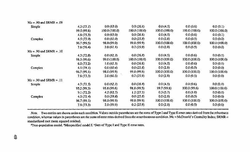
Mc = .9OandSRMR = .O9Simple

Complex

Mc = .90andSRMR = .10Simple

Complex

Mc = .90andSRMR = . l lSimple

Complex

4.3 (75.1)99.5 (99.8)4.8 (75.3)4.5 (75.9)

96.7 (99.5)7.8 (76.4)

4.3 (72.8)98.3 (99.6)6.0 (73.2)4.5(74.1)

96.7(99.1)7.8 (73.3)

4.3 (71.5)95.2 (99.3)

9.1 (72.2)4.5 (72.4)

96.7(99.1)7.8 (73.3)

0.0 (63.0)100.0(100.0)

0.0 (63.0)0.0 (61.0)

98.0(99.0)2.0(61.1)

0.0(62.3)99.0(100.0)

1.0(62.3)0.0 (60.4)

98.0 (99.9)2.0 (60.5)

0.0 (62.3)95.8 (99.6)

4.2 (62.7)0.0 (59.8)

98.0(99.9)2.0(59.9)

0.0(26.8)100.0(100.0)

0.0(26.8)0.0 (25.8)

99.8 (99.9)0.2 (25.9)

0.0(26.5)100.0(100.0)

0.0(26.8)0.0 (25.8)

99.8 (99.9)0.2 (25.9)

0.0 (26.8)98.8 (99.5)

1.2(27.3)0.0 (25.8)

99.8 (99.9)0.2 (25.9)

0.0(4.5)100.0(100.0)

0.0 (4.5)0.0 (2.8)

100.0(100.0)0.0(2.8)

0.0(4.5)100.0(100.0)

0.0(4.5)0.0(2.8)

100.0(100.0)0.0(2.8)

0.0(4.5)99.7 (99.8)0.3(5.7)0.0(2.8)

100.0(100.0)0.0(2.8)

0.0 (0.6)100.0 (100.0)

0.0 (0.6)0.0 (0.5)

100.0(100.0)0.0 (0.5)

0.0 (0.6)100.0(100.0)

0.0 (0.6)0.0 (0.5)

100.0(100.0)0.0 (0.5)

0.0 (0.6)100.0(99.6)

0.0(1.0)0.0 (0.5)

100.0(100.0)0.0(0.5)

0.0(0.1)100.0(100.0)

0.0 (0.1)0.0 (0.0)

100.0 (100.0)0.0 (0.0)

0.0(0.1)100.0(100.0)

0.0 (0.1)0.0 (0.0)

100.0(100.0)0.0 (0.0)

0.0 (0.1)100.0(100.0)

0.0(0.1)0.0 (0.0)

100.0(100.0)0.0 (0.0)

Note. Two entries are shown under each condition. Values outside parentheses are the sums of Type I and Type II error rates derived from the robustnesscondition, whereas values in parentheses are the sums of error rates derived from the nonrobustness condition. Me = McDonald's Centrality Index; SRMR =standardized root mean squared residual.

'True-population model. bMisspecified model I. cSum of Type I and Type II error rates.

CO

O1o

APPENDIX TABLE 10Rejection Rates (%) and the Sum of Type I and Type II Error Rates (%) for Simple and Complex True-Population Models and

Misspecified Models (I) Based on Combinational Rules With Me < .91 and SRMR > .06 (.07, .08, .09, .10, .11)

Cutoff Value

Me = .9 land SRMR = .06Simple

Complex

Me = .9 land SRMR = .07Simple

Complex

Me = .9 land SRMR = .08Simple

Complex

150

6.5' (92.9)lOO.O6 (100.0)

6.5C (92.9)5.8 (90.4)

93.8 (100.0)12.0 (90.4)

5.8 (87.1)100.0(100.0)

5.8 (87.1)5.8 (86.3)

100.0 (100.0)7.8 (86.3)

5.8 (81.6)100.0 (100.0)

5.8(81.6)5.8 (81.3)

98.0 (99.9)7.8 (81.4)

250

0.2 (75.5)100.0(100.0)

0.2 (75.5)0.2 (74.0)

99.3 (100.0)0.9 (74.0)

0.2 (70.6)100.0 (100.0)

0.2 (70.6)0.2 (69.6)

99.3 (100.0)0.9 (69.6)

0.2 (67.4)100.0(100.0)

0.2 (67.4)0.2 (66.6)

99.3 (100.0)0.9 (66.6)

500

0.0 (37.8)100.0 (100.0)

0.0 (37.8)0.0 (34.3)

100.0 (100.0)0.0 (34.3)

0.0 (37.3)100.0(100.0)

0.0 (37.3)0.0 (32.9)

100.0(100.000.0 (32.9)

0.0 (37.0)100.0 (100.0)

0.0 (37.0)0.0 (32.6)

100.0 (100.0)0.0 (32.6)

N

7,000

0.0(6.0)100.0(100.0)

0.0 (6.0)0.0(5.9)

100.0(100.0)0.0(5.9)

0.0 (6.0)100.0(100.0)

0.0(6.0)0.0(5.5)

100.0(100.0)0.0 (5.5)

0.0(6.0)100.0(100.0)

0.0 (6.0)0.0(5.5)

100.0(100.0)0.0 (5.5)

2,500

0.0 (0.6)100.0(100.0)

0.0 (0.6)0.0 (0.6)

100.0(100.0)0.0 (0.6)

0.0 (0.6)100.0(100.0)

0.0 (0.6)0.0 (0.6)

100.0(100.0)0.0 (0.6)

0.0 (0.6)100.0(100.0)

0.0 (0.6)0.0 (0.6)

100.0(100.0)0.0 (0.6)

5,000

0.0(0.1)1.5(100.0)0.0(0.1)0.0(0.1)

100.0(100.0)0.0(0.1)

0.0(0.1)100.0(100.0)

0.0(0.1)0.0(0.1)

100.0(100.0)0.0(0.1)

0.0(0.1)100.0(100.0)

0.0(0.1)0.0(0.1)

100.0(100.0)0.0(0.1)

Me = .91 and SRMR = .09Simple

Complex

Me = .91 and SRMR = .10Simple

Complex

Me = .91 and SRMR = .11Simple

Complex

5.8 (75.0)99.5 (99.8)6.3 (78.2)5.8 (77.8)

98.0 (99.8)7.8 (78.0)

5.8 (75.6)98.5 (99.8)7.3 (75.8)5.8 (76.0)

98.0(99.5)7.8 (76.5)

5.8 (74.4)95.7 (99.4)10.1 (75.0)5.8 (74.3)

98.0(99.5)7.8 (74.8)

0.2 (66.4)100.0 (100.0)

0.2 (66.4)0.2 (65.1)

99.3 (100.0)0.9 (65.1)

0.2 (65.6)99.0(100.0)

1.2(65.6)0.2 (64.5)

99.3 (100.0)0.9 (64.5)

0.2 (65.6)95.8 (99.6)

4.4 (66.0)0.2 (63.9)

99.3 (100.0)0.9(36.1)

0.0(56.9)100.0(100.0)

0.0(36.9)0.0 (32.4)

100.0 (100.0)0.0 (32.4)

0.0 (36.9)100.0(100.0)

0.0(36.9)0.0(52.4)

100.0 (100.0)0.0 (32.4)

0.0 (36.9)99.0 (99.8)

1.0(37.1)0.0 (32.4)

100.0(100.0)0.0(32.4)

0.0 (6.0)100.0(100.0)

0.0 (6.0)0.0 (5.5)

100.0 (100.0)0.0 (5.5)

0.0 (6.0)100.0 (100.0)

0.0 (6.0)0.0 (5.5)

100.0(100.0)0.0 (5.5)

0.0 (6.0)99.7 (99.1)

0.3 (6.9)0.0(5.5)

100.0(100.0)0.0(5.5)

0.0 (0.6)100.0(100.0)

0.0(0.6)0.0 (0.6)

100.0 (100.0)0.0 (0.6)

0.0 (0.6)100.0 (100.0)

0.0 (0.6)0.0 (0.6)

100.0(100.0)0.0(0.6)

0.0 (0.6)100.0 (99.6)

0.0 (1.0)0.0 (0.6)

100.0(100.0)0.0 (0.6)

0.0 (0.1)100.0(100.0)

0.0(0.1)0.0(0.1)

100.0(100.0)0.0(0.1)

0.0(0.1)100.0 (100.0)

0.0(0.1)0.0(0.1)

100.0(100.0)0.0(0.1)

0.0(0.1)100.0 (100.0)

0.0(0.1)0.0(0.1)

100.0(100.0)0.0(0.1)

Note. Two entries are shown under each condition. Values outside parentheses are the sums of Type I and Type II error rates derived from the robustnesscondition, whereas values in parentheses are the sums of error rates derived from the nonrobustness condition. Me = McDonald's Centrality Index; SRMR =standardized root mean squared residual.

"True-population model. bMisspecified model I. cSum of Type I and Type II error rates.

ro

APPENDIX TABLE 11Rejection Rates (%) and the Sum of Type I and Type II Error Rates (%) for Simple and Complex True-Population Models and

Misspecified Models (I) Based on Combinational Rules With RMSEA < .05 and SRMR > .06 (.07, .08, .09, .10, .11)

Cutoff Value

RMSEA = .05 and SRMR = .06Simple

Complex

RMSEA = .05 and SRMR = .07Simple

Complex

RMSEA = .05 and SRMR = .08Simple

Complex

150

4.7« (90.5)100.011 (100.0)

4.7* (90.5)4.7 (88.8)

98.8 (100.0)5.9 (88.8)

4.0 (84.1)100.0 (100.0)

4.0(84.1)4.7 (84.5)

96.7 (100.0)8.0 (84.5)

4.0 (78.4)100.0(100.0)

4.0 (78.4)4.7 (J9.4)

96.7 (99.9)8.0(79.5)

250

0.0(71.6)100.0 (100.0)

0.0 (71.6)0.0 (69.9) .

98.0(100.0)2.0 (69.9)

0.0 «5<5.S)100.0 (100.0)

0.0 (66.8)0.0 (65.5)

98.0 (99.9)2.0 (65.6)

0.0 (63.5)100.0(100.0)

0.0 (63.5)0.0 (62.5)

98.0 (99.9)2.0(62.6)

500

0.0(25.4)100.0 (100.0)

0.0 (25.4)0.0 (27.8)

99.8 (99.9)0.2 (27.9)

0.0(24.9)100.0(100.0)

0.0(24.9)0.0(26.4)

99.8 (99.9)0.2 (26.5)

0.0 (24.6)100.0(100.0)

0.0(24.6)0.0 (26.1)

99.8(99.9)0.2 (26.2)

N

1,000

0.0 (3.6)100.0(100.0)

0.0(3.6)0.0(3.3)

100.0(100.0)0.0 (3.3)

0.0(3.6)100.0(100.0)

0.0(3.6)0.0(2.9)

100.0(100.0)0.0 (2.9)

0.0(3.6)100.0(100.0)

0.0(3.6)0.0(2.9)

100.0(100.0)0.0(2.9)

2,500

0.0 (0.6)100.0(100.0)

0.0 (0.6)0.0 (0.5)

100.0(100.0)0.0 (0.5)

0.0 (0.6)100.0(100.0)

0.0 (0.6)0.0 (0.5)

100.0(100.0)0.0 (0.5)

0.0 (0.6)100.0(100.0)

0.0 (0.6)0.0 (0.5)

100.0(100.0)0.0 (0.5)

5,000

0.0(0.1)100.0(100.0)

0.0(0.1)0.0 (0.0)

100.0 (0.0)0.0 (0.0)

0.0 (0.1)100.0 (100.0)

0.0(0.1)0.0 (0.0)

100.0 (100.0)0.0 (0.0)

0.0(0.1)100.0(100.0)

0.0(0.1)0.0 (0.0)

100.0(100.0)0.0 (0.0)

RMSEA = .05 and SRMR = .09Simple

Complex

RMSEA = .05 and SRMR = . 10Simple

Complex

RMSEA = .05 and SRMR = .11Simple

Complex

4.0(74.5)99.5 (99.8)4.5 (74.7)4.7 (75.5)

96.7 (99.4)8.0(76.4)

4.0(72.^)98.3 (99.6)

5.7(72.5)4.7 (74.0)

96.7 (99.0)8.0(75.0)

4.0 (70.9)94.8 (99.3)

9.2(71.6)4.7 (72.3)

96.7 (99.0)8.0 (73.3)

0.0 (62.5)100.0(100.0)

0.0(62.5)0.0(67.0)

98.0(99.8)2.0(61.2)

0.0(<5/.<S)99.0(100.0)

1.0(61.8)0.0(60.4)

98.0(99.8)2.0(60.6)

0.0(67.S)95.8 (99.6)

4.2 (62.2)0.0(59.8)

98.0 (99.8)2.0 (60.0)

0.0 (24.5)100.0 (100.0)

0.0 (24.5)0.0 (25.9)

99.8 (99.9)0.2 (26.0)

0.0 (24.5)100.0(100.0)

0.0 (24.5)0.0(25.9)

99.8 (99.9)0.2 (26.0)

0.0(24.5)98.8 (99.5)

1.2(25.0)0.0(25.9)

99.8 (99.9)0.2 (26.0)

0.0 (3.6)100.0(100.0)

0.0 (3.6)0.0 (2.9)

100.0(100.0)0.0 (2.9)

0.0 (3.6)100.0 (100.0)

0.0 (3.6)0.0 (2.9)

100.0(100.0)0.0 (2.9)

0.0 (3.6)99.7 (98.8)

0.3 (4.8)0.0(2.9)

100.0(100.0)0.0(2.9)

0.0 (0.6)100.0 (100.0)

0.0 (0.6)0.0 (0.5)

100.0 (100.0)0.0 (0.5)

0.0 (0.6)100.0 (100.0)

0.0 (0.6)0.0 (0.5)

100.0 (100.0)0.0 (0.5)

0.0 (0.6)100.0 (99.6)

0.0(1.0)0.0 (0.5)

100.0 (100.0)0.0 (0.5)

0.0 (0.1)100.0 (100.0)

0.0(0.1)0.0 (0.0)

100.0 (100.0)0.0 (0.0)

0.0(0.1)100.0 (100.0)

0.0(0.1)0.0 (0.0)

100.0 (100.0)0.0 (0.0)

0.0(0.1)100.0(100.0)

0.0(0.1)0.0 (0.0)

100.0(100.0)0.0 (0.0)

Note. Two entries are shown under each condition. Values outside parentheses are the sums of Type I and Type II error rates derived from the robustnesscondition, whereas values in parentheses are the sums of error rates derived from the nonrobustness condition. RMSEA = root mean squared error ofapproximation. SRMR = standardized root mean squared residual.

"True-population model. bMisspecified model I. cSum of Type I and Type II error rates.

UiCO

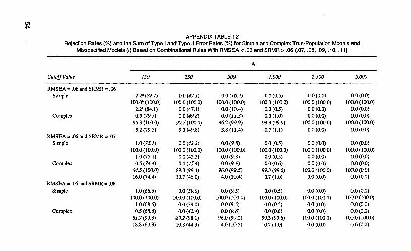
gAPPENDIX TABLE 12

Rejection Rates (%) and the Sum of Type I and Type II Error Rates (%) for Simple and Complex True-Population Models andMisspecified Models (I) Based on Combinational Rules With RMSEA < .06 and SRMR > .06 (.07, .08, .09, .10, .11)

Cutoff Value

RMSEA = .06 and SRMR = .06Simple

Complex

RMSEA = .06 and SRMR = .07Simple

Complex

RMSEA = .06 and SRMR = .08Simple

Complex

150

22'(84.1)100.0" (100.0)

2.2C(84.1)0.5 (79.5)

95.3 (100.0)5.2 (79.5)

1.0(75.7)100.0 (100.0)

1.0(75.1)0.5 (74.4)

84.5 (100.0)16.0(74.4)

1.0(68.6)100.0(100.0)

1.0(68.6)0.5 (68.6)

81.7(99.3)18.8 (69.3)

250

0.0(47.7)100.0(100.0)

0.0(47.1)0.0 (49.8)

90.7(100.0)9.3 (49.8)

0.0 (42.3)100.0(100.0)

0.0 (42.3)0.0 (45.4)

89.3 (99.4)10.7 (46.0)

0.0 (39.0)100.0(100.0)

0.0(39.0)0.0 (42.4)

59.2(98.1)10.8 (44.3)

500

0.0 (10.4)100.0(100.0)

0.0 (10.4)0.0 (11.3)

96.2 (99.9)3.8(11.4)

0.0 (9.8)100.0(100.0)

0.0 (9.8)0.0 (9.9)

96.0 (99.5)4.0(10.4)

0.0 (9.5)100.0 (100.0)

0.0 (9.5)0.0 (9.6)

96.0(99.1)4.0 (10.5)

N

7.000

0.0 (0.5)100.0(100.0)

0.0 (0.5)0.0(1.0)

99.3 (99.9)0.7(1.1)

0.0 (0.5)100.0(100.0)

0.0 (0.5)0.0 (0.6)

99.3 (99.6)0.7 (1.0)

0.0 (0.5)100.0(100.0)

0.0 (0.5)0.0 (0.6)

99.3 (99.6)0.7(1.0)

2.500

0.0(0.0)100.0(100.0)

0.0(0.0)0.0(0.0)

100.0(100.0)0.0(0.0)

0.0(0.0)100.0(100.0)

0.0(0.0)0.0(0.0)

100.0(100.0)0.0 (0.0)

0.0 (0.0)100.0 (100.0)

0.0 (0.0)0.0 (0.0)

100.0 (100.0)0.0 (0.0)

5,000

0.0 (0.0)100.0(100.0)

0.0 (0.0)0.0 (0.0)

100.0(100.0)0.0 (0.0)

0.0 (0.0)100.0(100.0)

0.0 (0.0)0.0 (0.0)

100.0(0.0)0.0(0.0)

0.0(0.0)100.0 (100.0)

0.0 (0.0)0.0 (0.0)

100.0 (100.0)0.0 (0.0)

RMSEA = .06 and SRMR = .09Simple

Complex

RMSEA = .06 and SRMR = .10Simple

Complex

RMSEA = .06 and SRMR = .11Simple

Complex

1.0 (64.8)99.5 (99.8)

1.5(65.0)0.5 (64.8)

81.7 (97.8)18.8 (67.0)

1.0 (62.3)98.3 (99.4)

2.7 (62.9)0.5 (63.0)

81.7(96.8)18.8 (66.2)

1.0(61.0)94.3 (98.8)

6.7 (62.2)0.5 (61.3)

81.7(96.3)18.8(65.0)

0.0(58.0)100.0(100.0)

0.0 (38.0)0.0(40.9)

89.2 (97.4)10.8 (43.5)

0.0(57.3)99.0(99.6)

1.0(37.7)0.0(40.3)

89.2 (97.0)10.8 (43.3).

0.0(57.5)95.7 (98.9)4.3 (38.4)0.0(39.6)

89.2 (96.6)10.8 (43.0)

0.0 (9.4)100.0 (100.0)

0.0 (9.4)0.0 (9.4)

96.0 (99.0)4.0(10.4)

0.0 (9.4)100.0(99.5)

0.0 (9.9)0.0 (9.4)

96.0 (99.0)4.0(10.4)

0.0(9.4)98.5 (97.6)

1.5(11.8)0.0(9.4)

96.0(99.0)4.0(10.4)

0.0 (0.5)100.0(100.0)

0.0(0.5)0.0 (0.6)

99.3 (99.6)0.7(1.0)

0.0 (0.5)100.0(100.0)

0.0 (0.5)0.0 (0.6)

99.3 (99.6)0.7(1.0)

0.0 (0.5)99.7 (98.5)

0.3 (2.0)0.0 (0.6)

99.3 (99.6)0.7(1.0)

0.0 (0.0)100.0 (100.0)

0.0 (0.0)0.0(0.0)

100.0(100.0)0.0 (0.0)

0.0 (0.0)100.0 (100.0)

0.0 (0.0)0.0 (0.0)

100.0(100.0)0.0 (0.0)

0.0 (0.0)100.0 (99.6)

0.0 (0.4)0.0 (0.0)

100.0(100.0)0.0 (0.0)

0.0 (0.0)100.0 (100.0)

0.0 (0.0)0.0 (0.0)

100.0 (100.0)0.0 (0.0)

0.0 (0.0)100.0(100.0)

0.0(0.0)0.0(0.0)

100.0 (100.0)0.0 (0.0)

0.0 (0.0)100.0(100.0)

0.0 (0.0)0.0 (0.0)

100.0(100.0)0.0 (0.0)

Note. Two entries are shown under each condition. Values outside parentheses are the sums of Type I and Type II errorrates derived from the robustnesscondition, whereas values in parentheses are the sums of error rates derived from the nonrobustness condition. RMSEA = root mean squared error ofapproximation. SRMR = standardized root mean squared residual.

"True-population model. bMisspecified model I. cSum of Type I and Type II error rates.