CurvesCurves

Chiew-Lan Tai

2

Curves

Reading

Required Hearn & Baker, 8-8 – 8-10, 8-12 Foley, 11.2

3

Curves

Curves Before Computers The loftsman’s or carpenter’s spline:

long, narrow strip of wood or metal shaped by lead weights called “ducks” Usually gives curves with second-order continuity

Used for designing cars, ships, airplanes etc.

But curves based on physical artefacts cannot be replicated well, since there is no exact definition of what the curve is.

Around 1960, a lot of industrial designers were working on this problem.

Today, curves are easy to manipulate on a computer and are used for CAD, art, animation, …

4

Curves

Motivation for curves

In graphics, what do we use curves for? creating models Paths of movement, animation

5

Curves

Curve Representations

Explicit y = f(x) what if the curve is not a function, e.g. a circle?

Implicit f(x,y,z) = 0x2 + y2 - R = 0

Parametric (x(u), y(u)) easier to work with

E.g. circle

x(u) = cos 2u

y(u) = sin 2u 0 u1

6

Curves

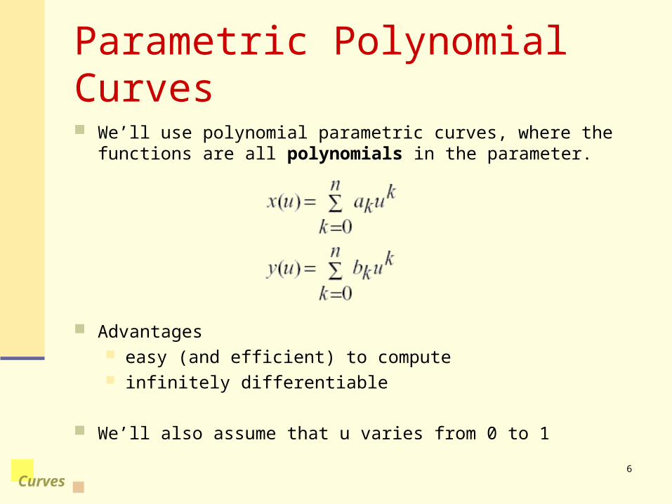
Parametric Polynomial Curves We’ll use polynomial parametric curves, where the functions are

all polynomials in the parameter.

Advantages easy (and efficient) to compute infinitely differentiable

We’ll also assume that u varies from 0 to 1

7

Curves

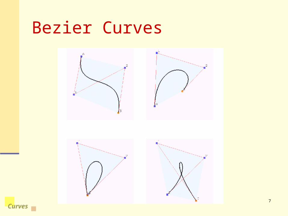
Bezier Curves

8

Curves

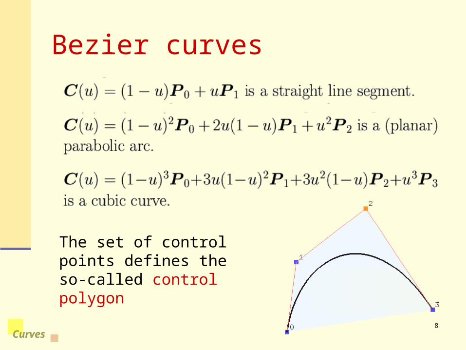
Bezier curves

The set of control points defines the so-called control polygon

9

Curves

deCasteljau’s algorithm

10

Curves

11

Curves

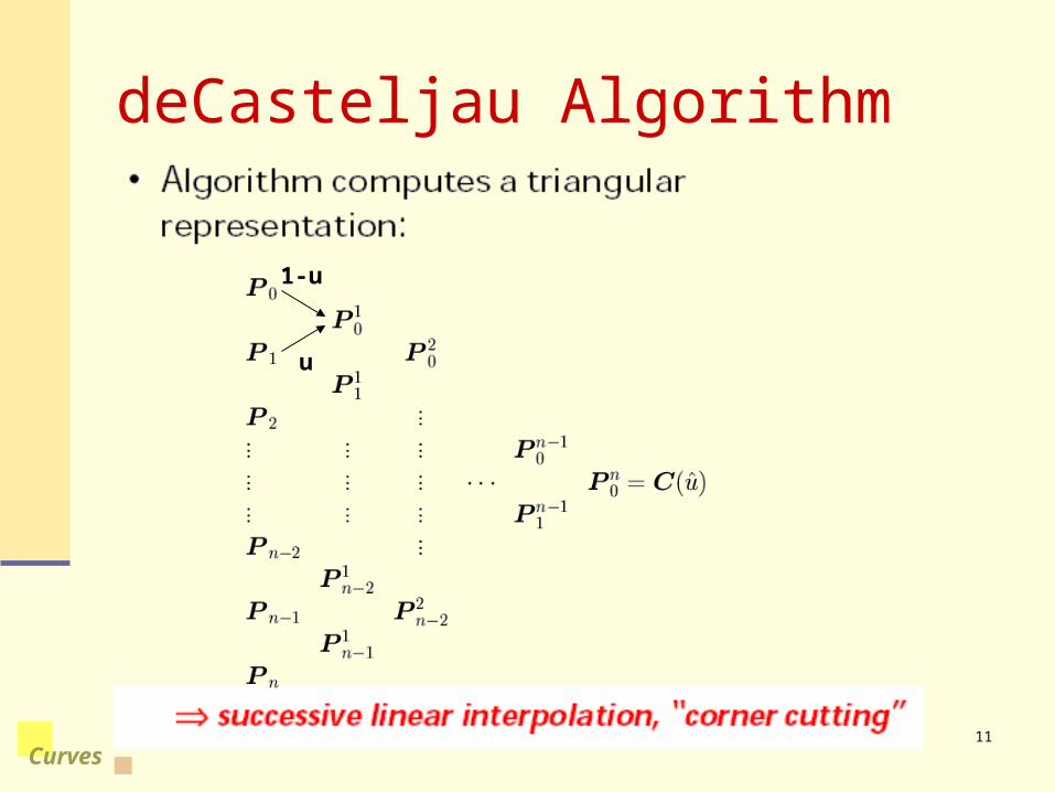
deCasteljau Algorithm

1-u

u

12

Curves

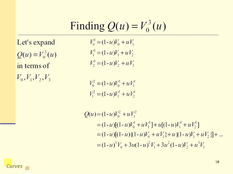
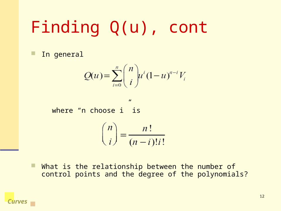
Finding Q(u), cont In general

where “n choose i” is

What is the relationship between the number of control points and the degree of the polynomials?

13

Curves

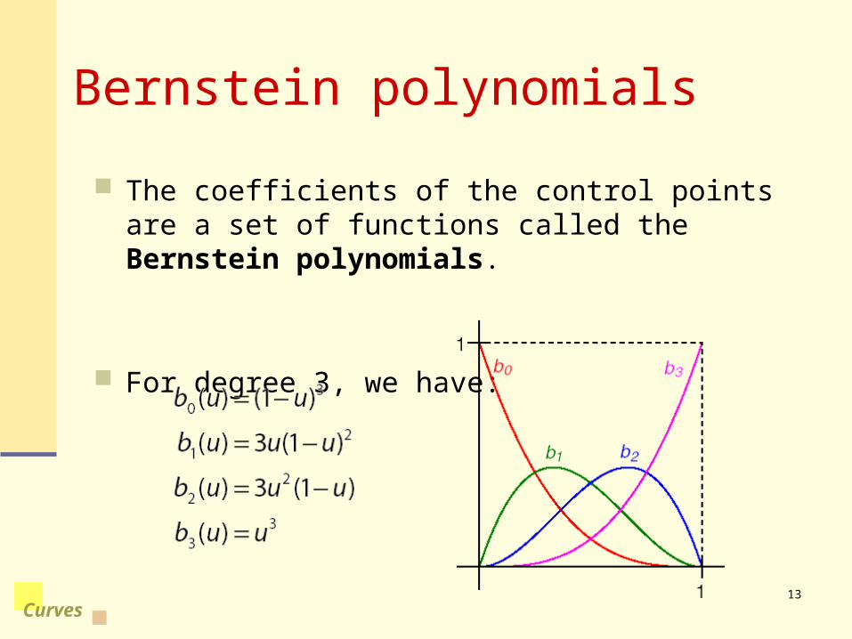
Bernstein polynomials

The coefficients of the control points are a set of functions called the Bernstein polynomials.

For degree 3, we have:

14

Curves

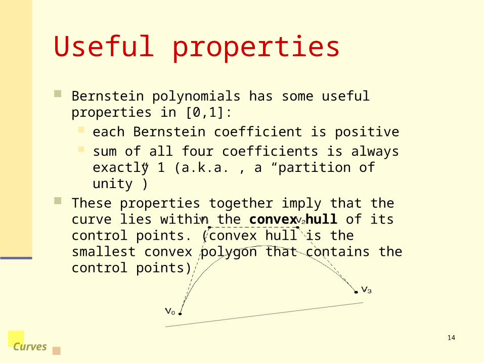
Useful properties

Bernstein polynomials has some useful properties in [0,1]: each Bernstein coefficient is positive sum of all four coefficients is always exactly 1 (a.k.a. ,

a “partition of unity”) These properties together imply that the curve lies within

the convex hull of its control points. (convex hull is the smallest convex polygon that contains the control points)

15

Curves

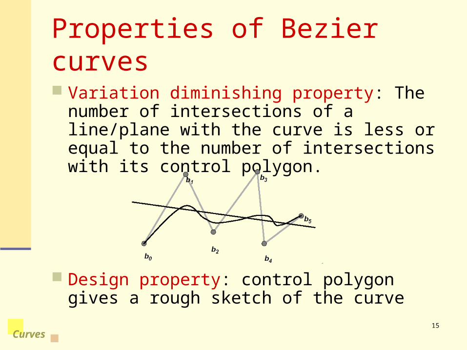
Properties of Bezier curves

Variation diminishing property: The number of intersections of a line/plane with the curve is less or equal to the number of intersections with its control polygon.

Design property: control polygon gives a rough sketch of the curve

16

Curves

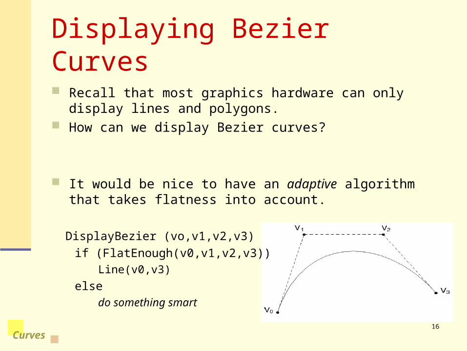
Recall that most graphics hardware can only display lines and polygons.

How can we display Bezier curves?

It would be nice to have an adaptive algorithm that takes flatness into account.

DisplayBezier (vo,v1,v2,v3)

if (FlatEnough(v0,v1,v2,v3))Line(v0,v3)

elsedo something smart

Displaying Bezier Curves

17

Curves

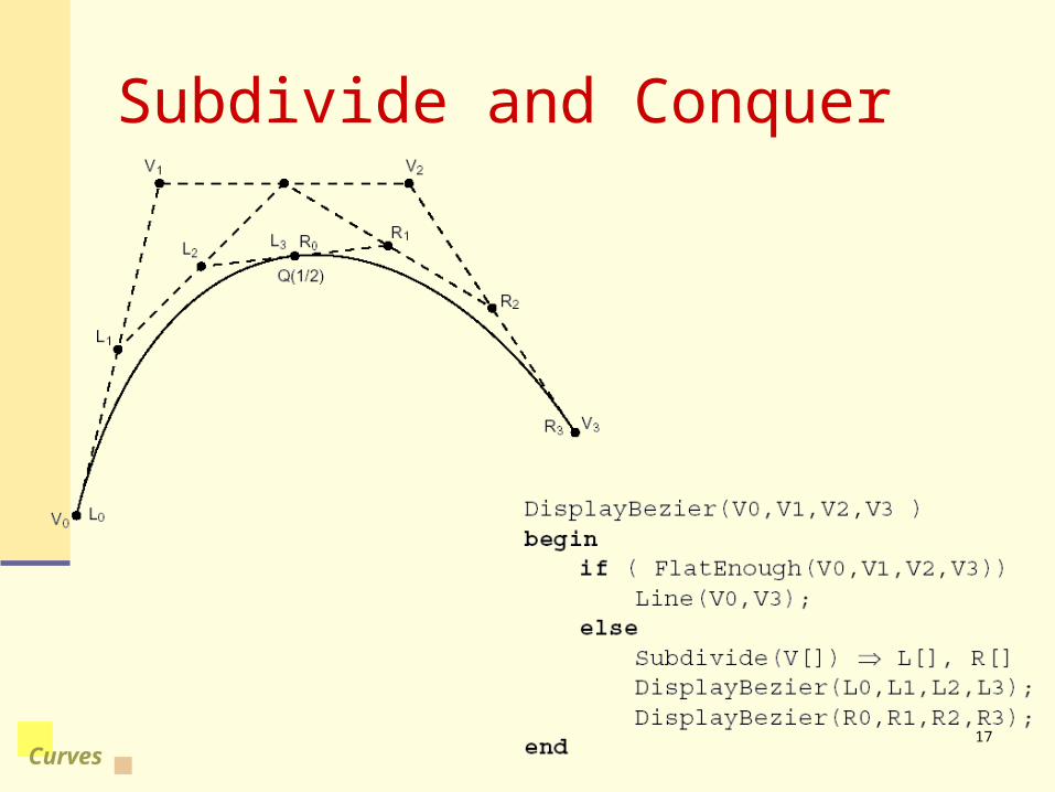
Subdivide and Conquer

18

Curves

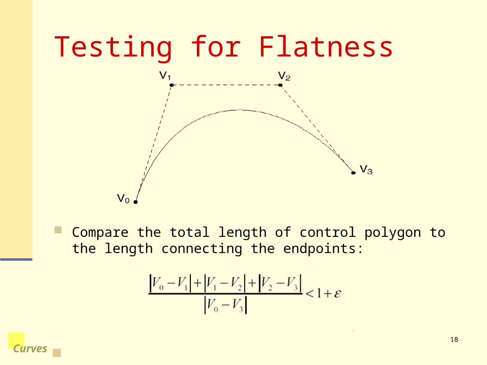
Testing for Flatness

Compare the total length of control polygon to the length connecting the endpoints:

19

Curves

More Complex Curves Suppose we want to draw a more complex curve.

We connect together individual curve segments that are cubic Bezier to form a longer curve, called splines.

Why cubic? Smallest degree curves that can represent curves in 3D

space

There are three properties that we’d like to have in our constructed splines … Local control Interpolation continuity

20

Curves

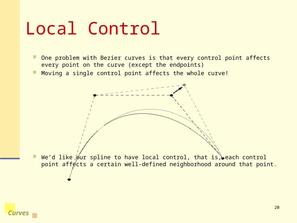
One problem with Bezier curves is that every control point affects every point on the curve (except the endpoints)

Moving a single control point affects the whole curve!

We’d like our spline to have local control, that is, each control point affects a certain well-defined neighborhood around that point.

Local Control

21

Curves

Interpolation

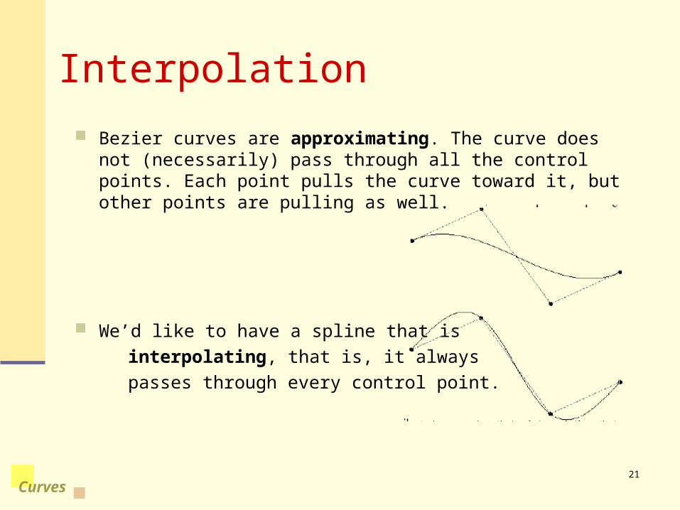
Bezier curves are approximating. The curve does not (necessarily) pass through all the control points. Each point pulls the curve toward it, but other points are pulling as well.

We’d like to have a spline that is

interpolating, that is, it always

passes through every control point.

22

Curves

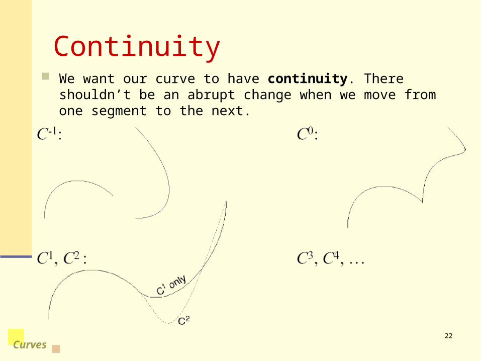
Continuity We want our curve to have continuity. There shouldn’t be an

abrupt change when we move from one segment to the next.

23

Curves

Ensuring Continuity

Let’s look at continuity first. Since the functions defining a Bezier curve are polynomials, all

their derivatives exist and are continuous on the interior of the curve.

Therefore, we only need to worry about the continuity at the endpoints of each curve segment (i.e., the joints).

24

Curves

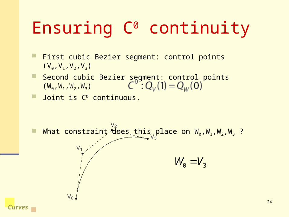
Ensuring C0 continuity

First cubic Bezier segment: control points (V0,V1,V2,V3)

Second cubic Bezier segment: control points (W0,W1,W2,W3)

Joint is C0 continuous.

What constraint does this place on W0,W1,W2,W3 ?

30 VW

25

Curves

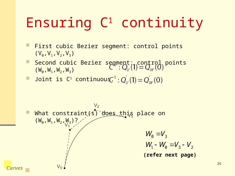
Ensuring C1 continuity

First cubic Bezier segment: control points (V0,V1,V2,V3)

Second cubic Bezier segment: control points (W0,W1,W2,W3)

Joint is C1 continuous.

What constraint(s) does this place on (W0,W1,W2,W3)?

2301

30

VVWW

VW

(refer next page)

26

Curves

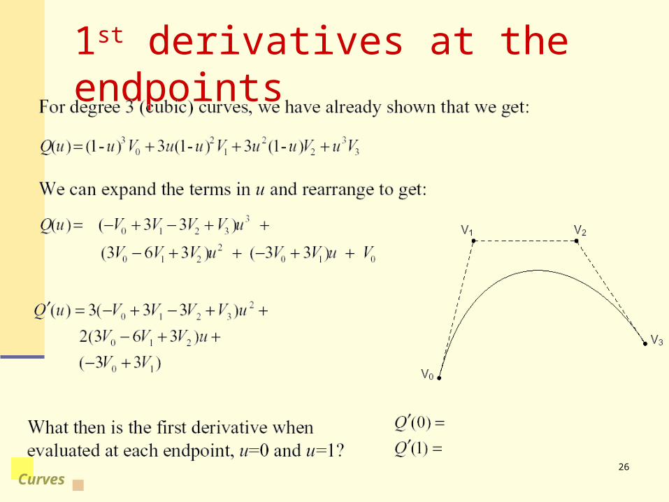
1st derivatives at the endpoints

27

Curves

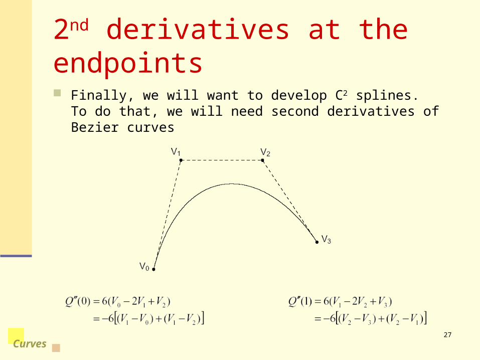
2nd derivatives at the endpoints Finally, we will want to develop C2 splines. To do that, we will

need second derivatives of Bezier curves

28

Curves

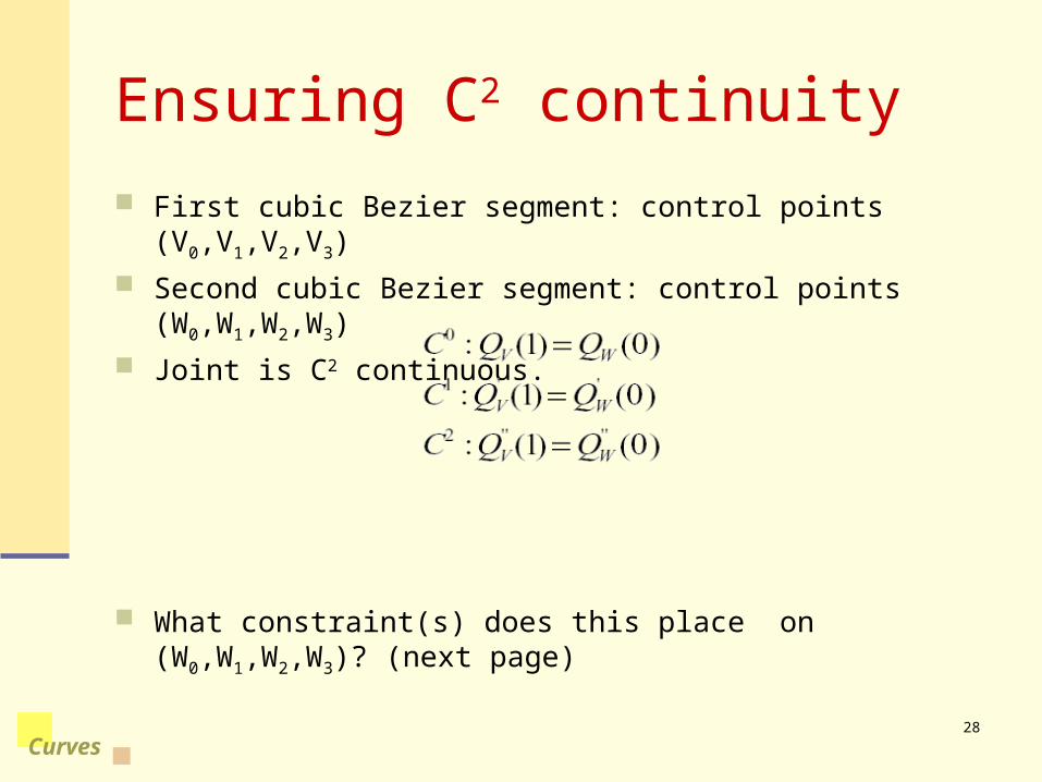
Ensuring C2 continuity

First cubic Bezier segment: control points (V0,V1,V2,V3)

Second cubic Bezier segment: control points (W0,W1,W2,W3)

Joint is C2 continuous.

What constraint(s) does this place on (W0,W1,W2,W3)? (next page)

29

Curves

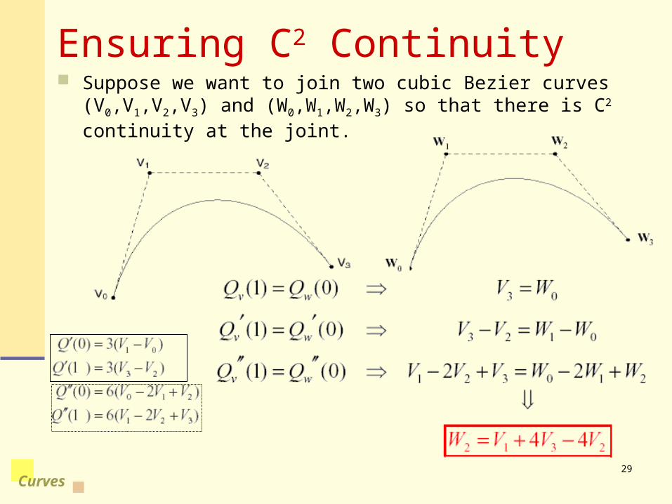
Ensuring C2 Continuity Suppose we want to join two cubic Bezier curves (V0,V1,V2,V3)

and (W0,W1,W2,W3) so that there is C2 continuity at the joint.

30

Curves

A-frames and Continuity

Let’s try to get some geometric intuition about what this last continuity equation means.

V

V

V

V

W

W

W W

31

Curves

Building a complex spline

Instead of specifying the Bezier control points themselves, let’s specify the corners of the A-frame in order to build a C2 continuous spline.

These are called B-splines. The Bi points are called de Boor points.

V0

V1 V2

V3

32

Curves

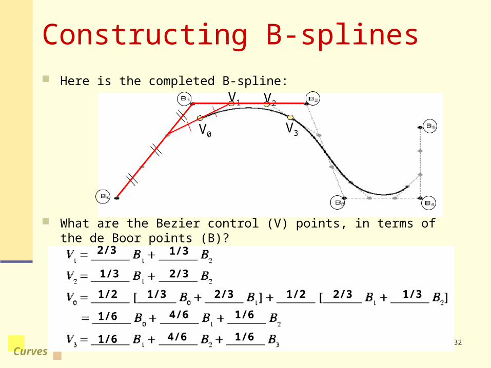
Constructing B-splines Here is the completed B-spline:

What are the Bezier control (V) points, in terms of the de Boor points (B)?

V0

V1 V2

V3

2/3 1/3

1/3 2/3

2/3 1/31/2 1/22/31/3

1/6 1/64/6

1/6 1/64/6

33

Curves

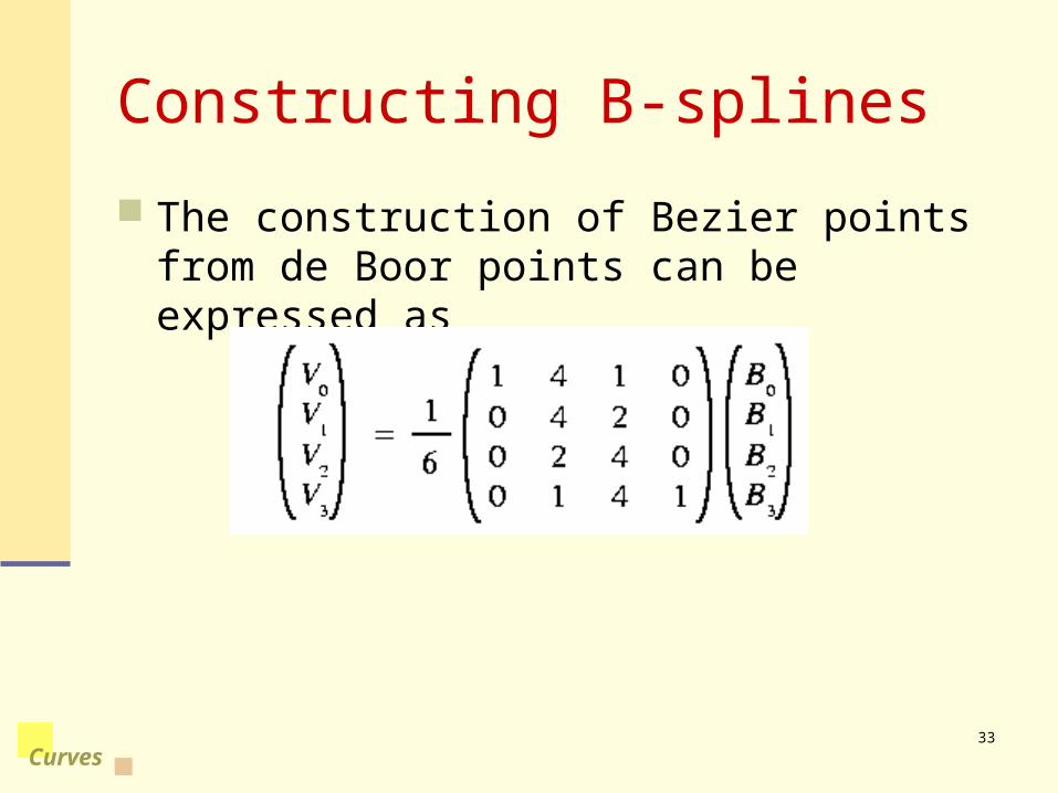
Constructing B-splines

The construction of Bezier points from de Boor points can be expressed as

34

Curves

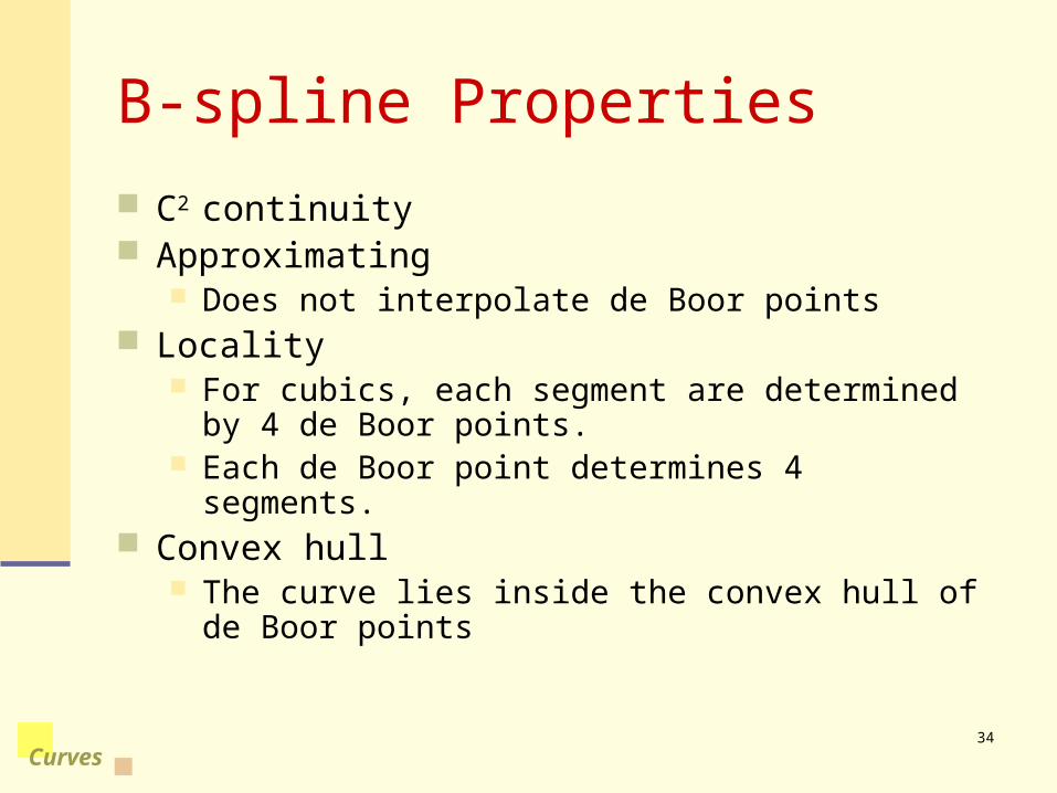
B-spline Properties

C2 continuity Approximating

Does not interpolate de Boor points Locality

For cubics, each segment are determined by 4 de Boor points.

Each de Boor point determines 4 segments. Convex hull

The curve lies inside the convex hull of de Boor points

35

Curves

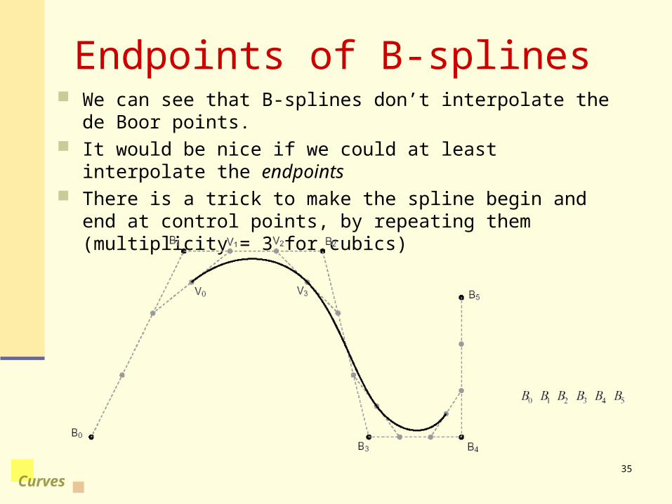
Endpoints of B-splines We can see that B-splines don’t interpolate the de Boor points. It would be nice if we could at least interpolate the endpoints There is a trick to make the spline begin and end at control

points, by repeating them (multiplicity = 3 for cubics)

36

Curves

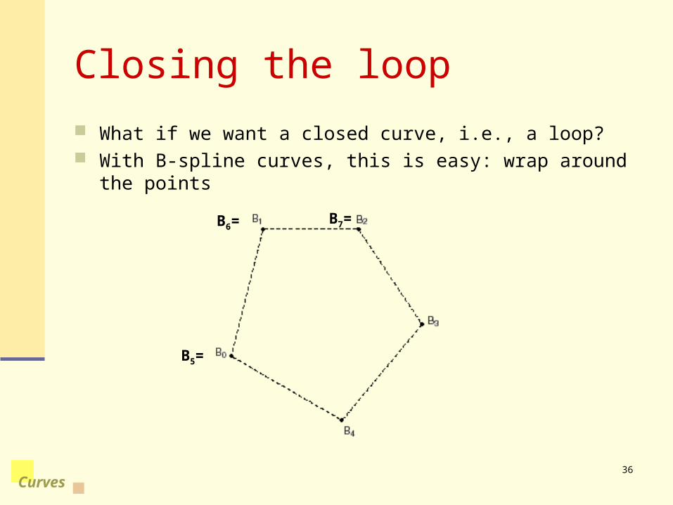
Closing the loop

What if we want a closed curve, i.e., a loop? With B-spline curves, this is easy: wrap around the points

B5=

B6= B7=

37

Curves

Displaying B-splines

Drawing B-splines is very simple:

DisplayBSpline (B0,B1,…,Bn)

for i = 0 to n-3Convert Bi,…,Bi+3 into Bezier control points V0, …, V3

DisplayBezier(V0,V1,V2,V3)

endfor

38

Curves

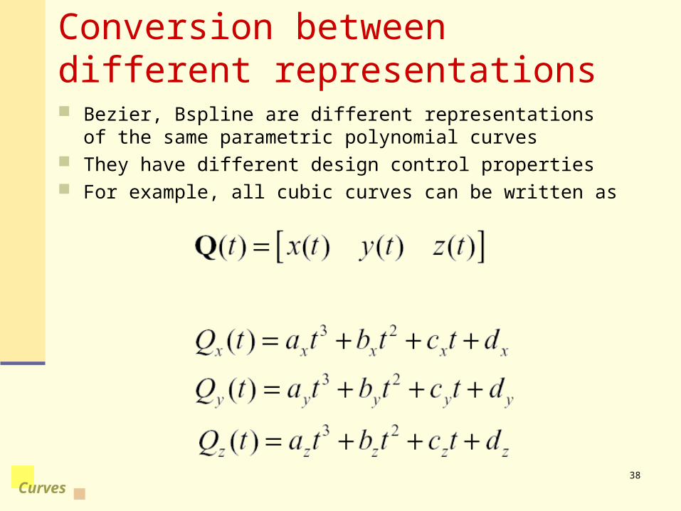
Conversion between different representations Bezier, Bspline are different representations of the same

parametric polynomial curves They have different design control properties For example, all cubic curves can be written as

39

Curves

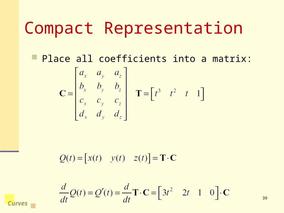
Compact Representation

Place all coefficients into a matrix:

40

Curves

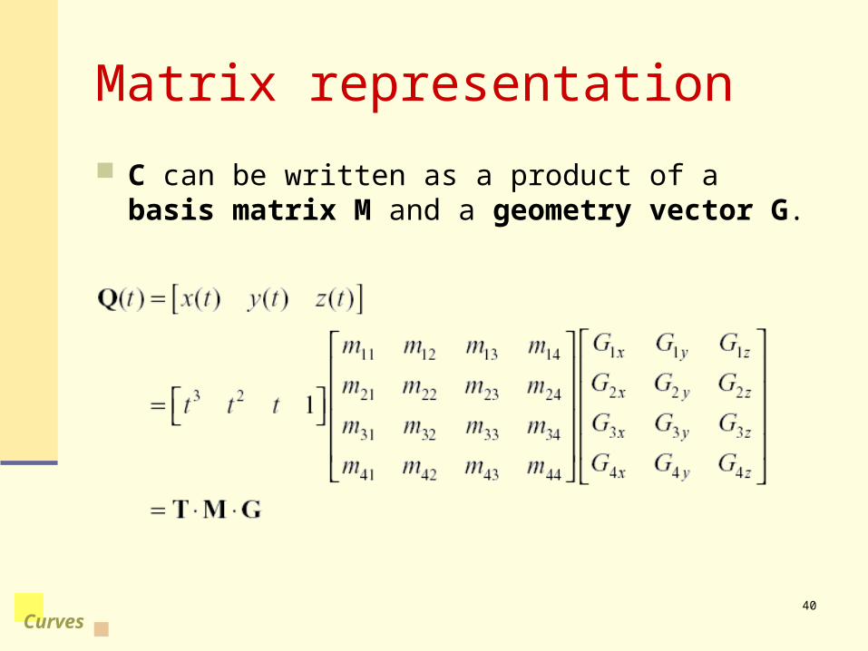
Matrix representation

C can be written as a product of a basis matrix M and a geometry vector G.

41

Curves

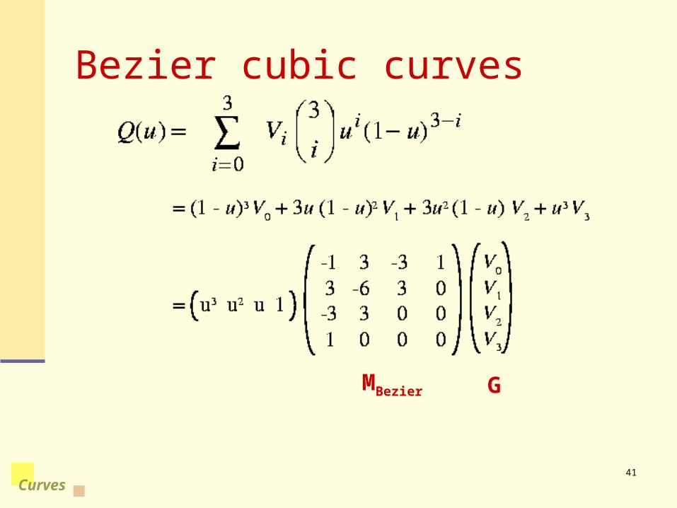
Bezier cubic curves

MBezier G

42

Curves

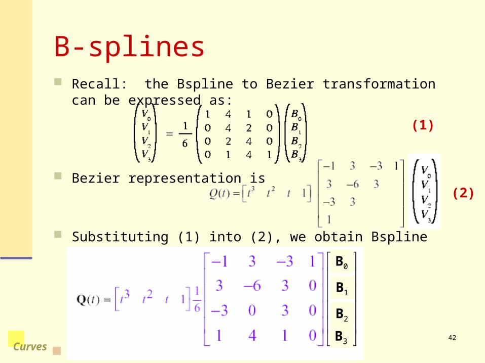
B-splines Recall: the Bspline to Bezier transformation can be expressed

as:

Bezier representation is

Substituting (1) into (2), we obtain Bspline representation:

B0

B1

B2

B3

(1)

(2)

43

Curves

Summary

What to take home from the lectures on curves: The meaning of all the bold face terms Definition and properties of Bezier curves How to display Bézier curves with line segments. Meanings of Ck continuities. Conditions for continuity of cubic splines. Construction of Bezier splines Definition, construction and properties of B-splines Matrix representation of curves Conversion between different representations

44

Curves

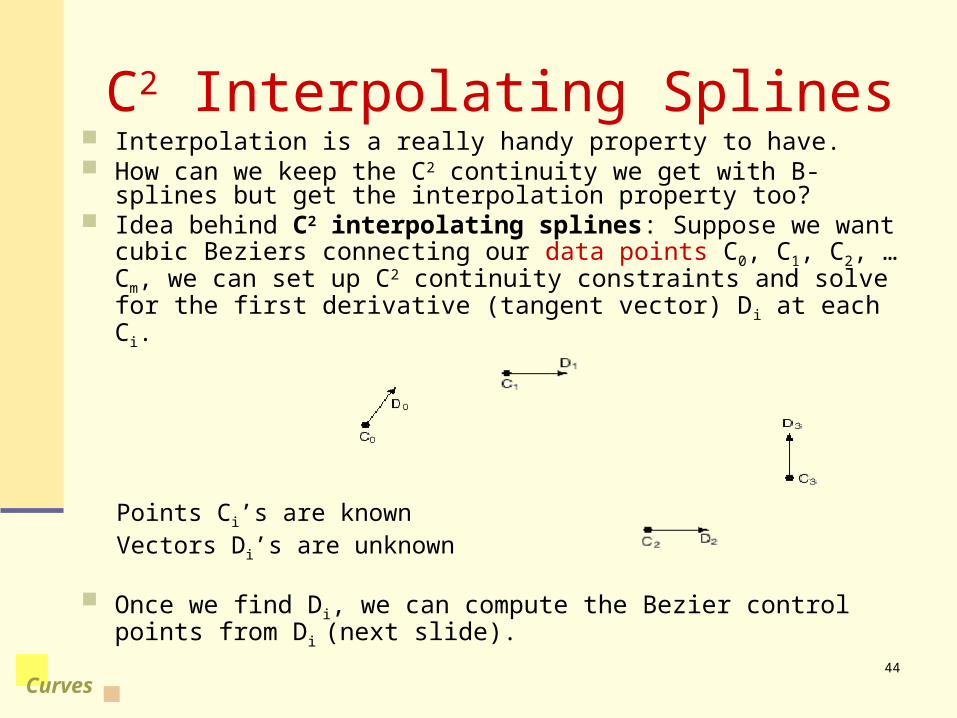
C2 Interpolating Splines Interpolation is a really handy property to have. How can we keep the C2 continuity we get with B-splines but get

the interpolation property too? Idea behind C2 interpolating splines: Suppose we want cubic

Beziers connecting our data points C0, C1, C2, …Cm, we can set up C2 continuity constraints and solve for the first derivative (tangent vector) Di at each Ci.

Once we find Di, we can compute the Bezier control points from Di (next slide).

Points Ci’s are knownVectors Di’s are unknown

45

Curves

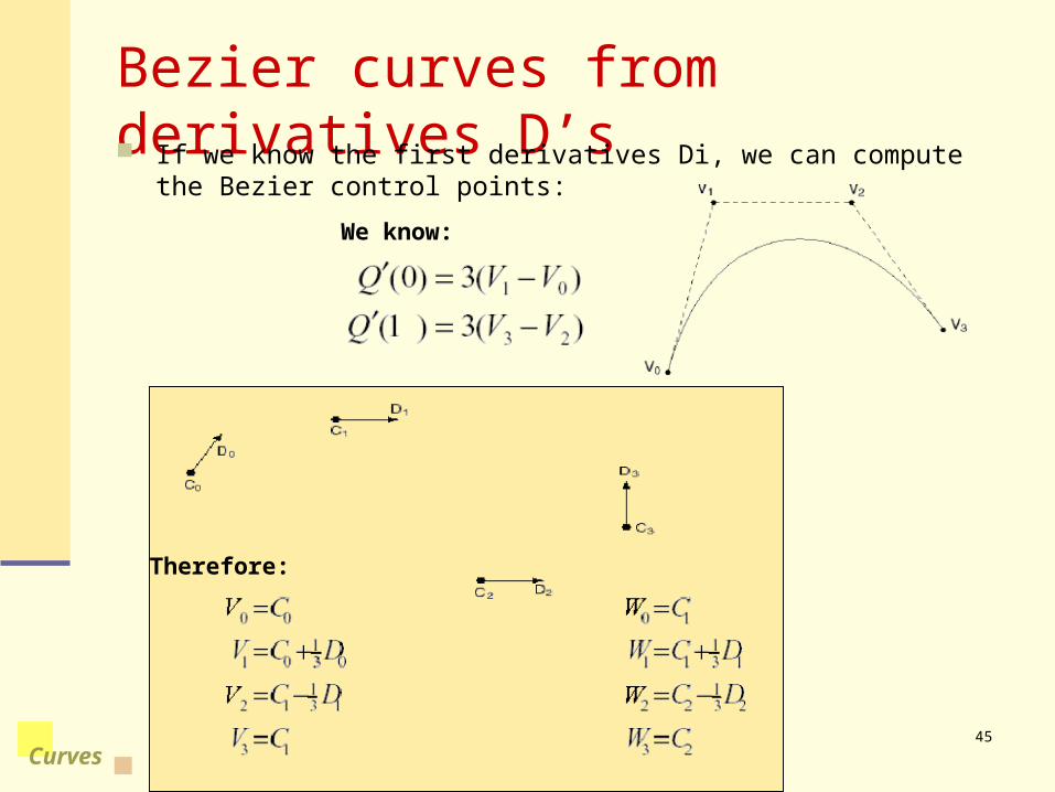
Bezier curves from derivatives D’s If we know the first derivatives Di, we can compute the Bezier control

points:

We know:

Therefore:

46

Curves

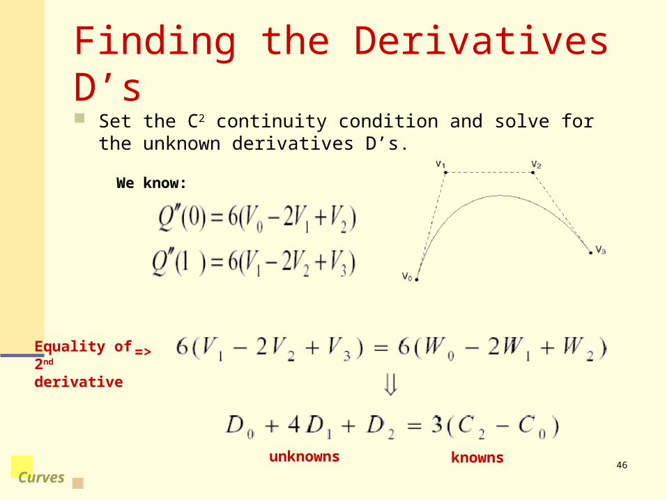
Finding the Derivatives D’s Set the C2 continuity condition and solve for the unknown

derivatives D’s.

Equality of 2nd derivative

=>

unknowns knowns

We know:

47

Curves

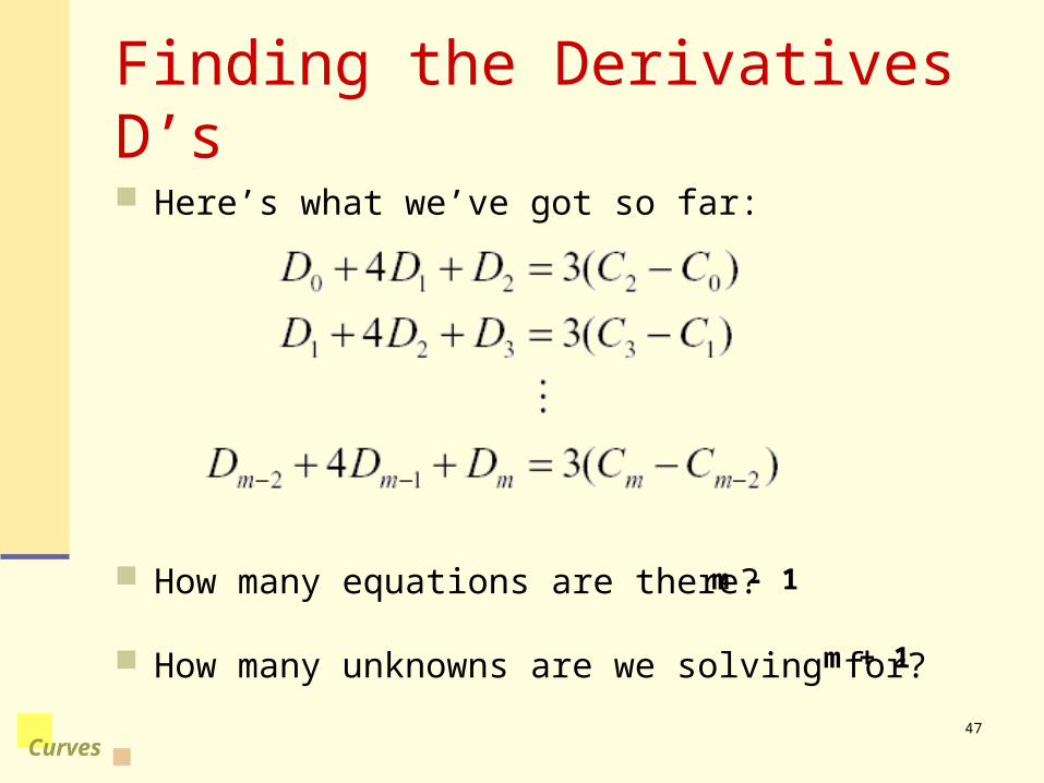
Finding the Derivatives D’s Here’s what we’ve got so far:

How many equations are there?

How many unknowns are we solving for?

m - 1

m + 1

48

Curves

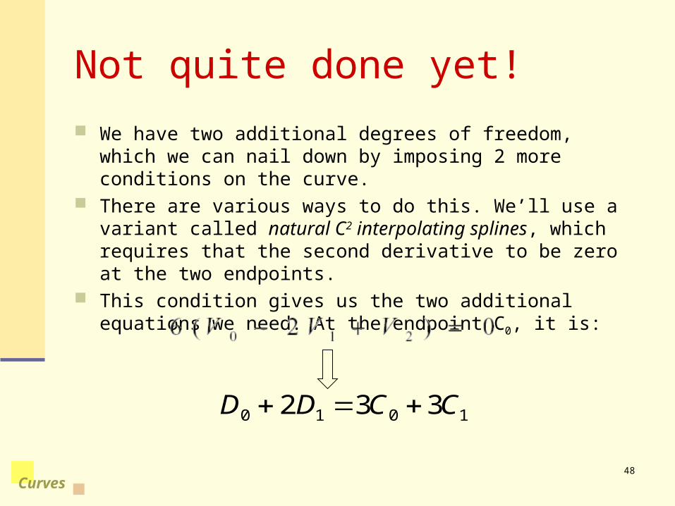
Not quite done yet!

We have two additional degrees of freedom, which we can nail down by imposing 2 more conditions on the curve.

There are various ways to do this. We’ll use a variant called natural C2 interpolating splines, which requires that the second derivative to be zero at the two endpoints.

This condition gives us the two additional equations we need. At the endpoint C0, it is:

1010 332 CCDD

49

Curves

Solving for the Derivatives

Let’s collect our m+1 equations into a single linear system:

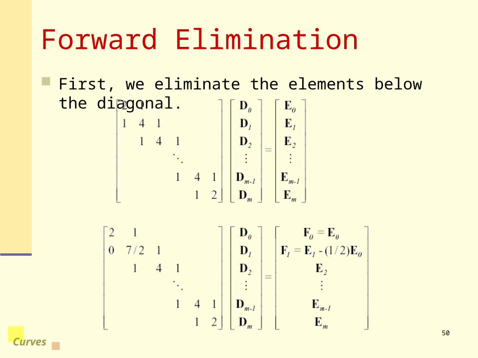
It’s easier to solve than it looks. We can use forward elimination to zero out everything below

the diagonal, then back substitution to compute each D value.

50

Curves

Forward Elimination First, we eliminate the elements below the diagonal.

51

Curves

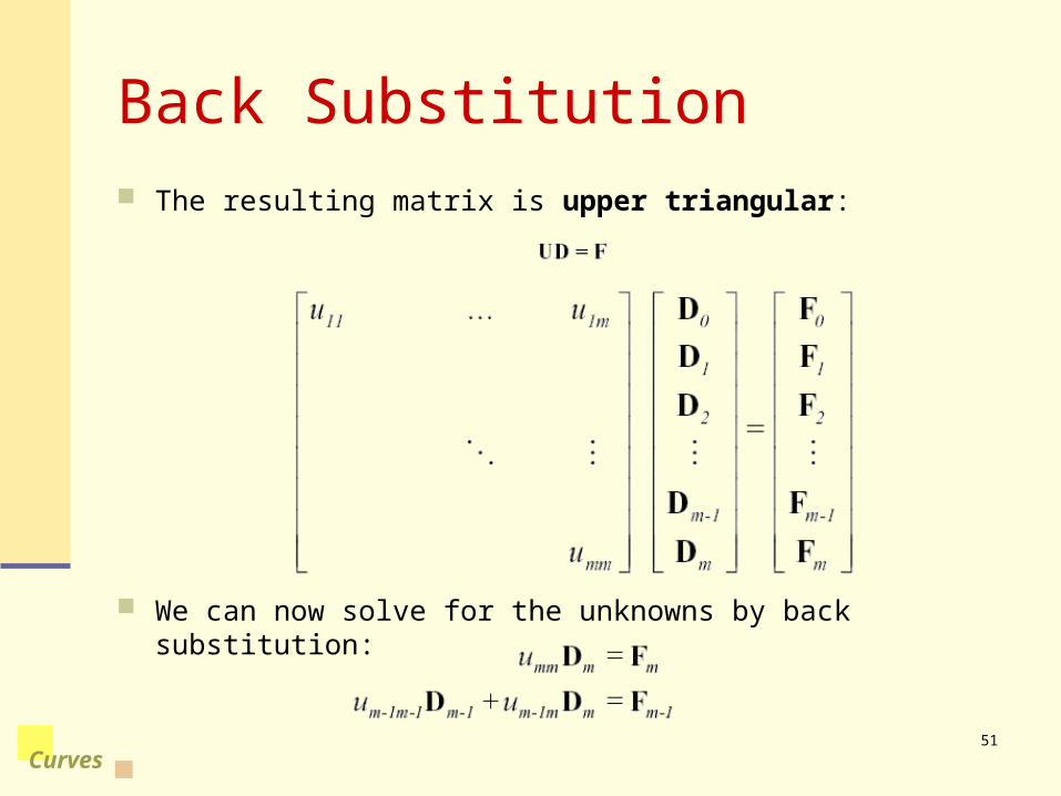
Back Substitution The resulting matrix is upper triangular:

We can now solve for the unknowns by back substitution:

52

Curves

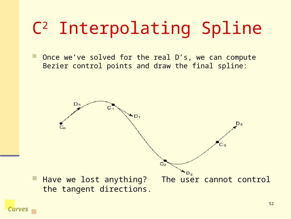
C2 Interpolating Spline Once we’ve solved for the real D’s, we can compute Bezier control

points and draw the final spline:

Have we lost anything? The user cannot control the tangent directions.