Curves before computers

The loftsman’s spline :

• Long, narrow strip of wood or metal

• Shaped by lead weights called ‘ducks’

• Gives curves with second-order continuity, ussually

Used for designed cars, ships, airplane, etc.

Motivation for Curves

What do we use curves for ?

• Building models

•Movement paths

• Animation

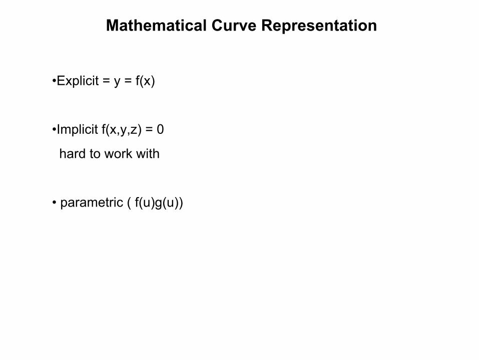
Mathematical Curve Representation

•Explicit = y = f(x)

•Implicit f(x,y,z) = 0

hard to work with

• parametric ( f(u)g(u))

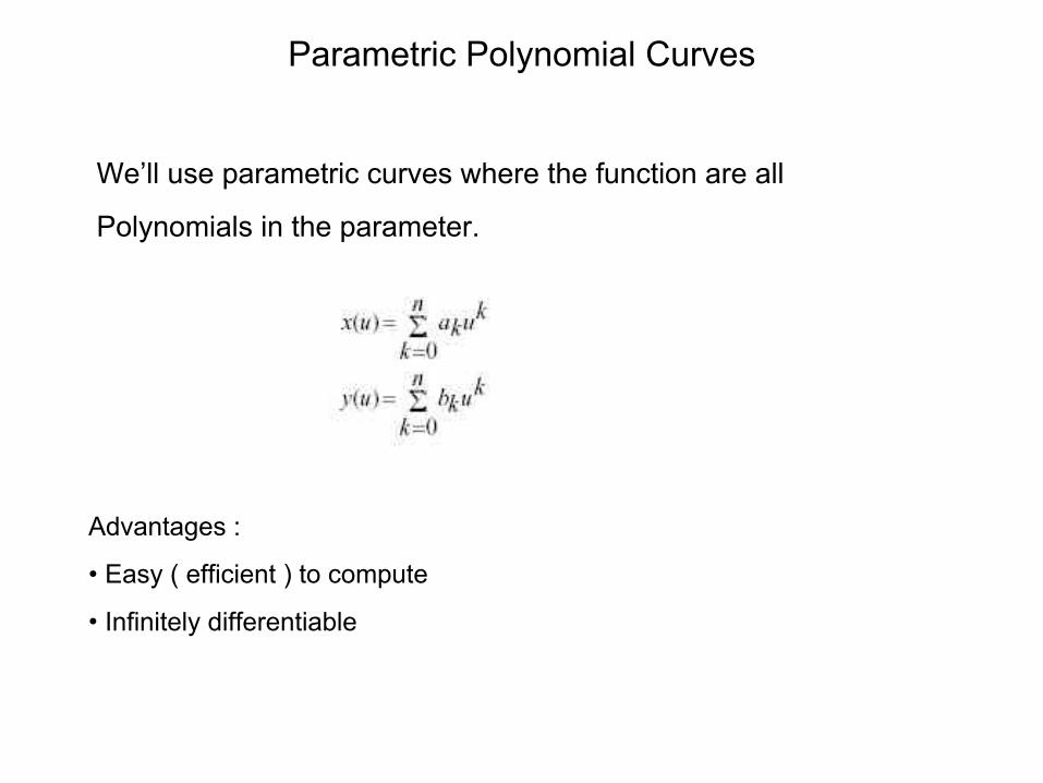
Parametric Polynomial Curves

We’ll use parametric curves where the function are all

Polynomials in the parameter.

Advantages :

• Easy ( efficient ) to compute

• Infinitely differentiable

Cubic Curves

Fix n = 3

For simplicity we define each cubic function within the range

Compact Representation

Place all cooficients into a matrix

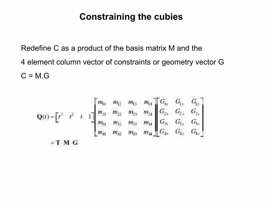
Constraining the cubies

Redefine C as a product of the basis matrix M and the

4 element column vector of constraints or geometry vector G

C = M.G

Hermite Curves

Determined by

• endpoints P1 and P4

• Tangent vectors at the endpoints R1 and R4

So

Computing Hermite basis matrix

The constraints on Q(0) and Q(1) are found by direct

Subtitution :

Collecting all constraints we get

Computing Hermite basis matrix

Computing a Points

Given two endpoints (P1,P4) and two endpoints tangents vectors

(R1,R4) :

Blending Function

Polynomials weighting each element of geometry vector

Continuity of Splines

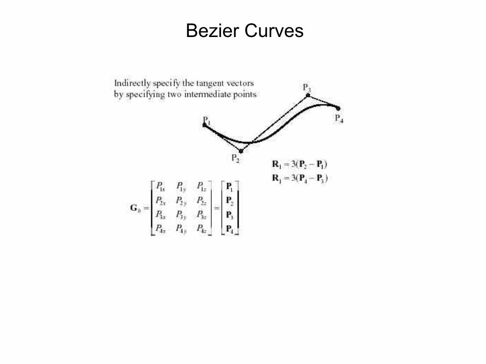
Bezier Curves

Bezier basis matrix

Bezier basis matrix

Bazier Blending function

Alternative Bezier Formulation

Displaying Bezier Curves

Subdivide and conquer

Testing for Flatness

More Complex CurvesSuppose we wants to draw a more complex curve

Why not use a high-order bezier ?

Instead , we’ll splice together a curve from individual segments that are cubic Bezier ?

Why Cubic ?

There are three properties we’d like to have in our newly constructed splines …………

Local ControlOne problem with Bezier is that every control point affects every point on the curve ( except the endpoints )

Moving a single control points affects the whole curve

We’d like our spline to have local control, that is, have each control point

Affect some well-defined neighborhood around that point.

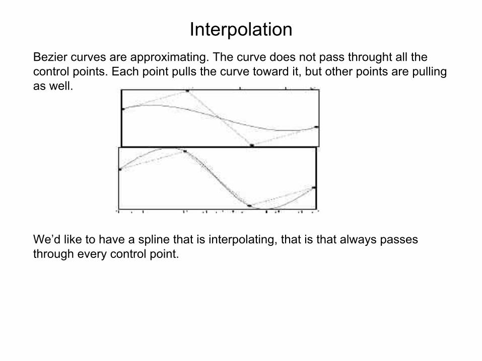
InterpolationBezier curves are approximating. The curve does not pass throught all the control points. Each point pulls the curve toward it, but other points are pulling as well.

We’d like to have a spline that is interpolating, that is that always passes through every control point.

ContinuityWe want our curve to have continuity. There shouldn’t be an abrupt change when we move from one segment to the next.

There are nested degrees of continuity

Ensuring continuity

Let’s look continuity first

Since the functions defining a bezier curve are polynomial,

All their derivatives exist and are continous.

Therefore, we only need to worry about the derivatives at the endpoints of the curve.

First, we’ll rewrite our equation for Q(t) in matrix form :

Derivatives at the endpoints

In general, the n derivatives at an endpoint depends only on the n+1 points nearest that endpoint.

Ensuring C2 continuitySuppose we have a cubic bezier defined by (V0,V1,V2,V3), and we want to attach another curve (W0,W1,W2,W3) to it.

So that there is C2 continuity at the joint.

A-Frames and continuity

Let’s try to get some geometrical intuition about what this last continuity equation means.

If a and b are points, what is ( 2a – b) ?

Building a complex spline

Instead of specifying the bezier control points themselves, let’s specify the corners of the A-frames in order to build a C2 continous spline.

These are called B-splines. The strating set of points are called de Boor points.

B-SplinesHere is the completed B-spline

What are the bezier control points , in terms of the de Boor points ?

Endpoints of B-splineWe can see that B-splines don’t interpolate the de Boor points.

It would be nice if we could at least control the endpoints of the splines explicity.

There’s a hack to make the spline begin and at control points by repeating them.

B-Spline matrix

C2 interpolating splines

Interpolation is a really handy property to have

How can we keep the C2 continuity we get with B-splines but get interpolation too ?

Here’s the idea behind C2 interpolation splines. Suppose we had cubic beziers connecting our control points C0,C1,C2,……….. And that we somehow knew the first derivative of the spline at each point

What are the V and W control points in term of Cs and Ds

Finding the derivatives

Now what we need to do is solve for the derivatives. To do this we’ll use the C2 continuity requirement.

Finding the derivatives, Here’s what we’ve got so far :

How many equation is this ?

How many unknowns are we solving for ?

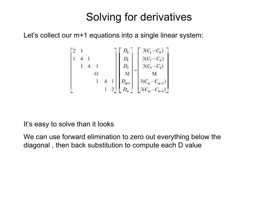
Solving for derivativesLet’s collect our m+1 equations into a single linear system:

It’s easy to solve than it looks

We can use forward elimination to zero out everything below the diagonal , then back substitution to compute each D value

C2 interpolating spline

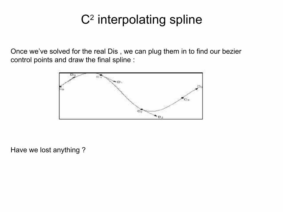
Once we’ve solved for the real Dis , we can plug them in to find our bezier control points and draw the final spline :

Have we lost anything ?

A third optionIf we’re willing sacrifice C continuity , we can get interpolation and local control .

Instead of finding the derivatives by solving a system of continuity equations, we’ll just pick something arbitrary but local.

If we set each derivatives to be constant multiple of the vector between the provious and next controls, we get a catmull-rom spline.

Catmull-rom splinesThe math for catmull-rom splines is pretty simple :

D0 = C1-C0

D1 = ½(C2-C0)

D2 = ½(C3-C1)

Dn = Cn-Cn-1

Catmull-Rom basis matrix