Curves and Surfaces

2

B-spline Curves

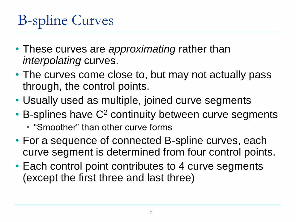
• These curves are approximating rather than interpolating curves.

• The curves come close to, but may not actually pass through, the control points.

• Usually used as multiple, joined curve segments

• B-splines have C2 continuity between curve segments• “Smoother” than other curve forms

• For a sequence of connected B-spline curves, each curve segment is determined from four control points.

• Each control point contributes to 4 curve segments (except the first three and last three)

3

B-spline Curves (2)

• By convention, curve segment Qi is determined by

control points Pi-3, Pi-2, Pi-1, and Pi

• Rather than defining each curve segment on the

interval 0 t 1, we make the parameter domains

sequential.

• Curve segment Qi is defined on the parameter range

ti t ti+1

• Between two curve segments Qi-1 and Qi there is a

join point or knot at parameter value ti

• A uniform B-spline has knots that are equally spaced

in t.

4

B-spline Curve Example

P0

P6

P5P4

P3

P2P1

t3

t7

t6

t5

t4

5

B-spline Geometry

• The B-spline geometry vector is given by

• The first curve segment, Q3 is defined by P0 to P3

over the parameter t3 = 0 to t4 = 1

• The second curve segment, Q4 is defined by P1 to P4

over the parameter t4 = 1 to t5 = 2

• The curve segment, Qm is defined by Pm-3 to Pm over the parameter tm = m-3 to tm+1 = m-2

i

i

i

i

BS

P

P

P

P

G

1

2

3

6

B-spline Properties

• Since each control point contributes to four curve segments, moving one control point alters four curve segments, but does not alter the others.

• Because of the way we have parameterized t, we define

• Then the curve segment is computed as

1)()()(23

iiiittttttT

1 ,)(

iiBsBsiitttGMTtQ

7

B-spline Properties

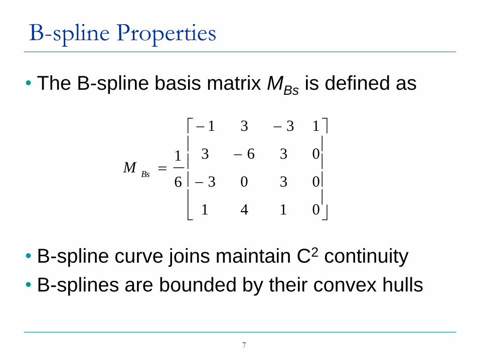
• The B-spline basis matrix MBs is defined as

• B-spline curve joins maintain C2 continuity

• B-splines are bounded by their convex hulls

0141

0303

0363

1331

6

1Bs

M

8

Drawing Curves

• Once we have the curves defined, how do we draw them?

• Two approaches:

1. Evaluate x(t), y(t), and z(t) for incrementally spaced values of t in an iterative fashion.

• Draw line segments between the points at each iteration

• Can optimize using Horner’s method or forward differences

2. Recursively subdivide the curve until the new control points get sufficiently close to the curve

• Can generate a large number of curve segments

9

Advantages of B-spline curves

• B-spline curves require more information and

a more complex theory than Bézier curves.

• But it has advantages to offset these

shortcomings.

• a B-spline curve can be a Bézier curve.

• B-spline curves satisfy all important properties that

Bézier curves have.

• B-spline curves provide more control flexibility than

Bézier curves can do.

10

Properties of B-spline curves

• We can change the position of a control point without

globally changing the shape of the whole curve.

• Since B-spline curves satisfy the strong convex hull

property, they have a finer shape control.

• There are other techniques for designing and editing

the shape of a curve such as changing knots.

• B-spline curves are still polynomial curves and

polynomial curves cannot represent many useful

simple curves such as circles and ellipses.

11

Localized Control

Moving the control point B7 only changes the curve near that point.

12

Problems with B-splines

• B-splines cannot represent conic sections

• In order to represent them, we can use a ratio

of polynomials

)(

)()(

2

1

tp

tptQ

13

NURBS

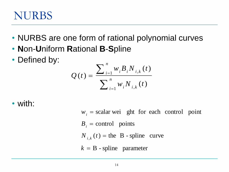
• NURBS are one form of rational polynomial curves

• Non-Uniform Rational B-Spline

• Defined by :

• its order

• determines the number of control points that affect a region of the curve

• The polynomial is degree one less than the order (i.e. order 4 is cubic polynomial)

• a set of weighted control points

• a knot vector

• a sequence of values that determine how the control points affect the curve

• NURBS curves are generalizations of both B-splines and Bezier curves

14

NURBS

• NURBS are one form of rational polynomial curves

• Non-Uniform Rational B-Spline

• Defined by:

• with:

n

i kii

n

i kiii

tNw

tNBwtQ

1 ,

1 ,

)(

)()(

parameter spline-B

curve spline-B the)(

points control

point controleach for ght scalar wei

,

k

tN

B

w

ki

i

i

15

NURBS

• If the weights are set to 1, the NURBS

becomes a regular B-spline

• NURBS can represent conics exactly.

16

Non-Uniform

Uniform Knot Vector

{0.0, 1.0, 2.0, 3.0, 4.0, 5.0, 6.0, 7.0}

Non-Uniform Knot Vector

{0.0, 1.0, 2.0, 3.75, 4.0, 4.25, 6.0, 7.0}

The knot intervals for B2 and B3:

{3.75, 4.0} and {4.0, 4.25} are narrower.

17

NURBS examples (from U of Calgary)

18

Parametric Bicubic Surfaces

• An extension to curves by adding another dimension

s = 0.2 s = 0.4s = 0.6 s = 0.8

s = 1.0s = 0.0

t = 0.0

t = 0.2

t = 0.4

t = 0.6

t = 0.8

t = 1.0

19

Curve Equation

• Remember, the equation of the curve is:

• Or, equivalently:

• Where G is the geometry vector, and s is a

constant

TMGtQ )(

SMGsQ )(

20

The Surface Equations

• If we allow G to be a function, we get

i.e., the geometry can now change, based on

t

)(

)(

)(

)(

)(),(

4

3

2

1

tG

tG

tG

tG

SMtSMGtsQ

21

The Surface Equations

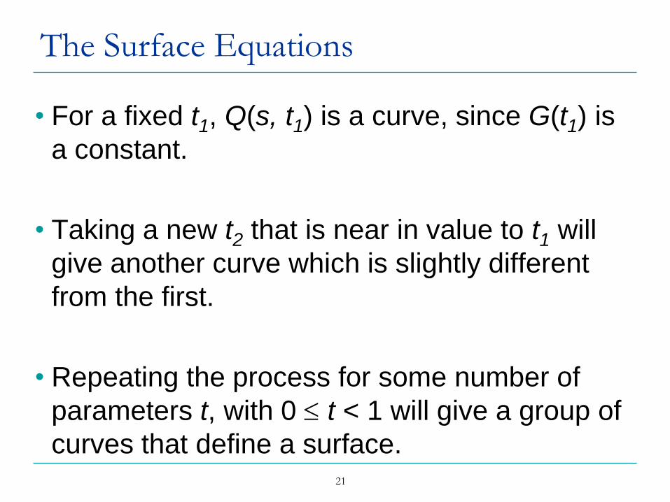
• For a fixed t1, Q(s, t1) is a curve, since G(t1) is

a constant.

• Taking a new t2 that is near in value to t1 will

give another curve which is slightly different

from the first.

• Repeating the process for some number of

parameters t, with 0 t < 1 will give a group of

curves that define a surface.

22

The Surface Equations

• Each of the Gi(t) functions are cubics, and can

be represented as:

• where

iiGTMtG )(

4

3

2

1

i

i

i

i

i

g

g

g

g

G

23

Surface Equations

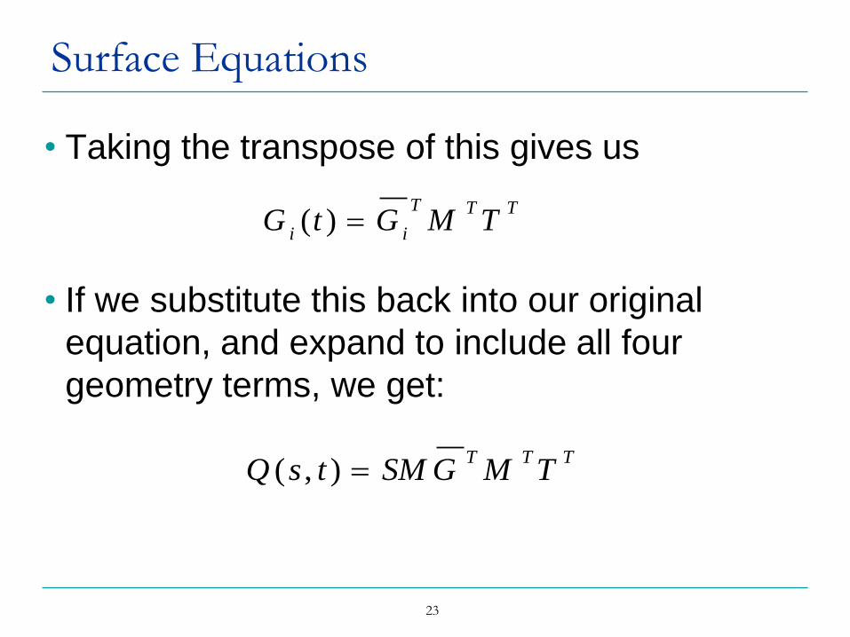
• Taking the transpose of this gives us

• If we substitute this back into our original

equation, and expand to include all four

geometry terms, we get:

TTT

iiTMGtG )(

TTTTMGSMtsQ ),(

24

Surface Equations

• So,

• With being the geometry matrix and M

being the basis matrix.

TTT

xTMGSMtsx ),(

TTT

yTMGSMtsy ),(

TTT

zTMGSMtsz ),(

G

25

Bezier Surfaces

• The ends of each patch require 4 control

points in the s direction.

• The t direction gives rise to 4 control points

also

• Thus, there are 4x4 or 16 control points

required for each patch.

26

Bezier Surface Example

27

Joining Bezier Surfaces

• Multiple Bezier

surfaces can be

joined with C0

continuity by:

• Making the four

control points at the

join common

between the two

patches

P11

P33

P23

P22P32

P21P31

P41

P42

P43

P12

P13

P14P44

P34P24

P17

P16

P15

P47

P37

P27

P46

P36P26

P45

P35P25

28

Joining Bezier Surfaces

• To join with C1

continuity we must

also enforce the

following stipulations:

1. The control points on

either side of the join

must be collinear

2. All of the pairs of line

segments joining the

three collinear control

points must have

lengths that have the

same ratios

P11

P33

P23

P22P32

P21P31

P41

P42

P43

P12

P13

P14P44

P34P24

P17

P16

P15

P47

P37

P27

P46

P36P26

P45

P35P25

29

Joining Bezier Surfaces

• For this example

the following ratios

must be equal:

P11

P33

P23

P22P32

P21P31

P41

P42

P43

P12

P13

P14P44

P34P24

P17

P16

P15

P47

P37

P27

P46

P36P26

P45

P35P254544

4443

3534

3433

2524

2423

1514

1413

PP

PP

PP

PP

PP

PP

PP

PP

30

Displaying Surfaces

• Surfaces are displayed in a manner similar

to curves.

1. Iteratively evaluate the surface equation at s and t

intervals, then draw polygons for those patches

2. Subdivide the surface until the patch size is small

enough

31

NURBS Surfaces

• NURBS –

• Non Uniform

• - knots can have any spacing desired

• Rational

• the blending functions are the ratios of two polynomials

• B-Spline

• the surface type is B-spline

• Very flexible and powerful

• Also somewhat complex

• Can represent conics exactly

• Used extensively, particularly in CAD

32

NURBS Examples

http://www.geomagic.com

33

http://gallery.mcneel.com/

34

http://gallery.mcneel.com/

35

http://gallery.mcneel.com/

36

NURBS in OpenGL

gluNurbsSurface(GLUnurbs *nurb,

Glint sKnotCount,

GLfloat *sKnots,

Glint tKnotCount,

GLfloat *tKnots,

Glint sStride,

Glint tStride,

GLfloat *control,

Glint sOrder,

Glint tOrder,

GLenum type)

37

NURBS in OpenGL

• nurb – specifies the NURBS object –created with gluNewNurbsRenderer

• sKnotCount –number of knots in the s direction

• sKnots – the array of s knots

• tKnotCount – number of knots in the t direction

• tKnots – the array of t knots

• sStride – offset between control points in the s direction

• tStride – offset between control points in the t direction

• control – array of control points

gluNurbsSurface(GLUnurbs *nurb,

Glint sKnotCount,

GLfloat *sKnots,

Glint tKnotCount,

GLfloat *tKnots,

Glint sStride,

Glint tStride,

GLfloat *control,

Glint sOrder,

Glint tOrder,

GLenum type)

• sOrder – order of the NURBS in s

• tOrder – order of the NURBS in t

• type – type of surface

38

Trimming Curves

• Sometimes we want “holes” in the surface

• Can define them using trimming curves

• Define a NURBS curve on the NURBS surface

• Draw the surface everywhere except inside

the curve

39

40

41

Subdivision Surfaces

• One problem with the surfaces we have

discussed is the difficulty in changing

resolution for a portion of the surface

• If we want more detail at one part of the patch,

we have to introduce a whole new patch

• Subdivision surfaces allow local refinement of

the control mesh

• This gives more flexibility in the objects to be

modeled

42

Subdivision Surfaces

• Idea: recursively subdivide the patch to finer

and finer resolution

Refinement 1 Refinement 2

Refinement ∞

43

Standard Subdivision

• Given initial control points, recursively

subdivide until desired smoothness is reached

44

Adaptive Subdivision

• Generally some areas of the surface have

higher curvature, and thus should be

subdivided further than other areas

• Can apply an adaptive subdivision scheme to

subdivide more where we want finer control of

the surface

45

Adaptive Subdivision Surface Example

from http://grail.cs.washington.edu/projects/subdivision/

Original Mesh After one refinement

After two refinements The limit – infinite refinement

46

Subdivision Surfaces

Geri’s Game (1997) : Pixar Animation Studios

47

Subdivision Surface Example

http://mrl.nyu.edu/~dzorin/sig98course/multires/sld005.htm

48

Allowing for Sharp Edges and Creases

• Often we want to permit

sharp edges

• How can we smooth

some of the surface, but

not all?

• Tag edges as sharp or

non-sharp

• If an edge is sharp, apply

sharp subdivision rules

• Otherwise apply normal

subdivision rules

49

T-splines

• Introduced by Dr. Sederberg in 2003

• Allow T-junctions in the surfacesT-junction

50

T-Splines

51

T-spline Hole Filling

52

T-spline example

53

Summary

• Surfaces allow for a higher level of realism

• Used in all CAD packages

• NURBS surfaces are the most popular type

• Subdivision surfaces allow for increased

surface detail, and for local adaptation

• T-splines allow for even more flexibility