Embed Size (px)
Citation preview

1
A Demand System Analysis of the U.S. Trout Market
YOUNGJAE LEE
Department of Agricultural Economics and Agribusiness Louisiana State University AgCenter
101 Agricultural Administration Building Baton Rouge LA 70803-5606
Phone: 225-578-2754 Fax: 225-578-2716
E-Mail: [email protected]
P. LYNN KENNEDY
Department of Agricultural Economics and Agribusiness Louisiana State University AgCenter
101 Agricultural Administration Building Baton Rouge LA 70803-5606
Phone: 225-578-2726 Fax: 225-578-2716
E-Mail: [email protected]
BRIAN M. HILBUN
Department of Agricultural Economics and Agribusiness Louisiana State University AgCenter
101 Agricultural Administration Building Baton Rouge LA 70803-5606
Phone: 225-578-0345 Fax: 225-578-2716
E-Mail: [email protected]
Selected Paper prepared for presentation at the Southern Agricultural Economics Association Annual Meeting, Orlando, FL, February 6-9, 2010
Copyright 2010 by Youngjae Lee, P. Lynn Kennedy, and Brian Hilbun. All rights reserved. Readers may make verbatim copies of this document for non-commercial purposes by any means, provided that this copyright notice appears on all such copies.
2
A Demand System Analysis of the U.S. Trout Market
Youngjae Lee, P. Lynn Kennedy, and Brian Hilbun
Faced with a dynamic change in U.S. trout imports, this study tried to identify how trout imports affect the domestic trout industry in the United States. In doing so, this study analyzed the quantity effect and exchange rate effect on domestic trout price using a modified LDI-AIDS model. According to the results of this study, we found five important facts related to trout imports during this sample period of time. First, a low farm price of domestic trout might be due to reasons other than trout imports because empirical results show that the net effects of imported trout products are complementary rather than substitutionary in effect. Second, domestic trout price decreases with an increase in total trout supply into domestic market. Third, imported frozen products are gross-substitutes for domestic product, while imported fresh products are gross-complements for domestic product. Fourth, for domestic trout, the intensity of substitutable interaction of imported products is as follows: frozen fillets > frozen whole trout > fresh whole trout > rainbow trout. Finally, depreciation of the U.S. Dollar relative to the Chilean Peso reduces the negative impact of Chilean imported trout on domestic trout price.
Although the domestic nominal price of trout has increased at an annual rate of 2.01% from 1991
to 2008, the real price for domestic trout has decreased because inflation for that time period was
3.26%. The decrease in the real price of domestic trout might be one of the reasons for the
decrease in domestic production of trout during this period of time. In contrast, along with an
increase in demand for value added trout products, trout imports have increased from 1,754 to
4,165 tons, which, in turn, caused the market share of imported trout to increase from 6.5% in
1991 to 17.5% in 2008. In addition to an increase in imports, there is a dynamic change in trout
imports in terms of types of value added trout products, origins, and prices. According to trade
codes for U.S. imports, representative products of imported trout are: 1) frozen fillets (HS:
0304206005), 2) fresh or chilled whole trout (HS: 0302110090), 3) frozen whole trout (HS:
0303210000), and 4) farmed fresh rainbow trout (HS: 0302110010).1
Frozen fillets represent the largest share of imported trout, accounting for 57% of total
imports in 2008. However, the import share of the frozen fillets has decreased from a high of

3
74% in 1991. The major exporting country of frozen fillet changed from Argentina to Chile. In
2008, Chilean frozen fillet takes 64.7% of total frozen fillet imports. Argentina exports 72.1% of
total frozen fillet in 1991 but only 27.6% in 2008. From 1991 to 2008, the price of frozen fillet
has the most highly increased from $2.03 per kilogram to $5.29 per kilogram. One reason of this
increase of price comes from the devaluation of the U.S. currency against the currencies of
exporting countries in recent years. For example, the value of one U.S. dollar was 691 Chilean
Pesos in 2003 but only 462 Chilean Pesos in 2008.
Import share for fresh whole trout has increased from 12.7% in 1991 to 18.4% in 2008.
This increase may be related to the recent wider culinary adoption of trout in the general cuisine,
e.g., the increased popularity of trout steaks.2 The major exporting country of fresh whole trout
is Canada which has a geographical advantage for the export of perishable products into the
United States as compared to other exporting countries. Canadian share of fresh whole trout
imports into the U.S. has increased from 62.8% in 1991 to 70.2% in 2008. Chilean fresh whole
trout commanded a 21.1% share of fresh whole trout imports in 1991 but only a 2.6% share in
2008. The imported fresh trout price is higher than those for frozen fillets and frozen whole
trout. From 1991 to 2008, the prices of imported fresh whole trout have increased from $4.15 per
kilogram to $6.20 per kilogram. The recent U.S. currency value against the Canadian dollar also
decreased from Canadian dollar 1.57/$ in 2002 to Canadian dollar 0.87/$ in 2008.
Import share of frozen whole trout has decreased from 12.1% in 1991 to 6.4% in 2008.
The major exporting country of frozen whole trout is Chile. The Chilean share of U.S. imported
frozen whole trout has increased slightly from 50.1% in 1991 to 54.7% in 2008. Canadian share
has expanded from 4.5% in 1991 to 22.2% in 2008. The price of imports of frozen whole trout is

4
lower than for those of either imported trout fillets or fresh trout. The prices of imported frozen
whole trout have increased from $3.77 per kilogram in 1991 to $4.19 per kilogram in 2008.
Although the relative size of import volumes of farmed fresh rainbow trout is small, the
import share of farmed fresh rainbow trout has markedly increased from 1.2% in 1991 to 17.8%
in 2008. It might be related to the recent increasing preference for value added trout products.
The major exporting country of farmed fresh rainbow trout is Canada. However, the Canadian
share of farmed fresh rainbow trout imports has decreased from 82.3% in 1991 to 67.4% in 2008.
This lost Canadian market share has been absorbed by growth in the Latin American export
market to the United States. From 1991 to 2008, the price of imported farmed fresh rainbow trout
has increased from $4.56 per kilogram to $6.24 per kilogram.
As previously mentioned, trout imports have changed dynamically since 1991. The
objective of this study is to describe how imported trout affects the domestic U.S. trout industry.
Also, this study examines the effect of the exchange rate on the domestic U.S. trout price using
trade theory to explain the fundamental relationship between currency value and prices for both
the importer and exporter.3 In doing so, this study uses the Differential Inverse Almost Ideal
Demand System (DIAIDS) which will be modified according to the objective of this study.
This study proceeds as follows. The next section discusses model development. In section
three, we discuss data and estimation. Section four discusses the estimated results. Finally, the
paper will conclude by providing the major findings of this study.
Duality and the Linear Inverse Demand System
To derive an inverse demand system, one can start either from the direct utility function and
exploit Wald’s identity which yields uncompensated inverse demands, or start from the distance

5
(transformation) function and exploit Shephard’s theorem which yields compensated inverse
demand functions (Weymark, 1980 and Kim, 2001).
If ( )qU is a direct utility function, where q denotes the vector of quantities, the
transformation or distance function ( )quD , is implicitly defined by ( )[ ] uquDqU ≡,/ , where u is
the reference utility level. The distance function is continuous, increasing, linearly homogeneous,
and concave with respect to q , and decreasing inu . These properties establish a useful parallel
between the distance function and the expenditure function, ( )puE , , derived from the utility-
constrained expenditure minimization problem (where p is the price vector corresponding to q ).
The parallel features of expenditure and distance functions are useful because, as
emphasized by Hanoch (1978), they imply that any standard functional form for the expenditure
function can be applied also to the distance function. The derivation of the linear inverse almost
ideal demand system(LIAIDS) model starts with an expenditure function, exchanging the role of
the variables ( )pu, in the PIGLOG expenditure function of the AIDS model with the variables
( )qu,− with that of the distance function, where the negative sign on u emphasizes the opposite
monotonic direction of ( )quD , and ( )puE , relative to the utility index. Then, the expenditure
function given reference utility u is:
(1) ( ) ( ) ( )qubqaD −=ln ,
where ( )qa and ( )qb are quantity aggregator functions defined as:
(2) ( ) ( ) ( ) ( )∑∑∑ ++=i j
jiiji
ii qqqqa lnln21ln0 γαα ,
and
(3) ( ) ∏=i
iiqqb ββ0 .
6
Because at 1=D , the distance function is an implicit form of the direct utility function,
then (1) implies the utility function ( ) ( ) ( )qbqaqU /= . This, together with the derivative property,
implies that the uncompensated inverse demand functions associated with (1)-(3) can be written
in share form as:
(4) ( ) ( )∑ −+=j
ijijii Qqw *lnln βγα ,
where iii qw π≡ is the ith budget share, and ( )*ln Q is a quantity index defined as ( ) ( )qaQ ≡*ln .
Equation (2) and (4) together entail a nonlinear structure for the inverse demand model.
In practice, however, ( )*ln Q can be replaced by an index ( ) ( )∑= i ii qwQ lnln constructed prior
to estimation of the share system to yield LIAIDS as:
(5) ( ) ( )∑ −+=j
ijijii Qqw lnln βγα .
Fortunately, an alternative exists, the first-difference LIAIDS, that is,
(6) ( ) ( )∑ +=j
ijiji Qdcqdcdw lnln .
The resulting set of (6) is a linear differential inverse almost ideal demand system (LDIAIDS).
In (6), the adding up, homogeneity, and symmetry conditions of ijc and ic can be
defined as follows:
Adding up: 0=∑i ijc and 0=∑i ic ;
Homogeneity: 0=∑ j ijc ;
Symmetry: jiij cc = .
The quantity and scale elasticities can be derived from (6) as follows:
(7.1) jijiijij wwcf +−= δ/* : compensated quantity elasticity

7
(7.2) 1/ −= iii wcf : scale elasticity
(7.3) ijijij fwff += * : uncompensated quantity elasticity.
Data and Estimation
Data Description
Our analyses include domestic food-size trout, imported frozen trout fillets, fresh whole trout,
frozen whole trout, and farm raised rainbow trout. We obtained annual price and quantity data of
these products for the period beginning in January 1991 to 2008 from various sources. Price and
quantity data for domestic food-size trout were obtained from the National Agricultural Statistics
Service (NASS). Quantity and value data for imported trout were obtained from the National
Marine Fisheries Service (NMFS). The unit prices of imported trout were obtained by dividing
the total value by volume of imports.
The obtained quantity and price data represent an actual quantity like pounds or
kilograms and an actual price like dollars per pound or kilogram. Before using these actual data
in an estimating procedure, we manipulated these data without sacrificing their original
properties in the following manner. At first, we calculate the weighted average of quantity of
these products during the sample period of time as follows:
(8) TNQ
Q i t it
×= ∑ ∑ ,
where itQ is the actual quantity of product i at time t, N represents the number of commodities
(N = 5 in this study) and T represents the number of months in the study period (T = 18 in this
study). Then, the normalized quantity of seafood product i at each time t is obtained as follows:
(9) QQ
q ii = ,

8
where iq is the normalized quantity of product i. iq is greater than one if iQ > Q . iq is less
than one if iQ < Q . And iq is equal to one if iQ = Q . Furthermore, the normalized quantity,
iq , has the same property of actual quantity, iQ , in terms of their relative size.
Now, we normalize the actual price, p , as follows. We first recalculate expenditure using
normalized quantity and is expressed as follows:
(10) ∑= i iiqpx .
Using (3), we normalize product i price as follows:
(11) xpi
i =π .
Using (4), we then obtain normalized budget share of product i as follows:
(12) iii qw π= .
And the normalized expenditure, the sum of the normalized budget share, will be one:
(13) 1=∑i iw .
Normalized quantity, price, and budget share will be directly (as itself) or indirectly (as
logarithmic or differencing logarithmic number) used in the estimating procedure. The
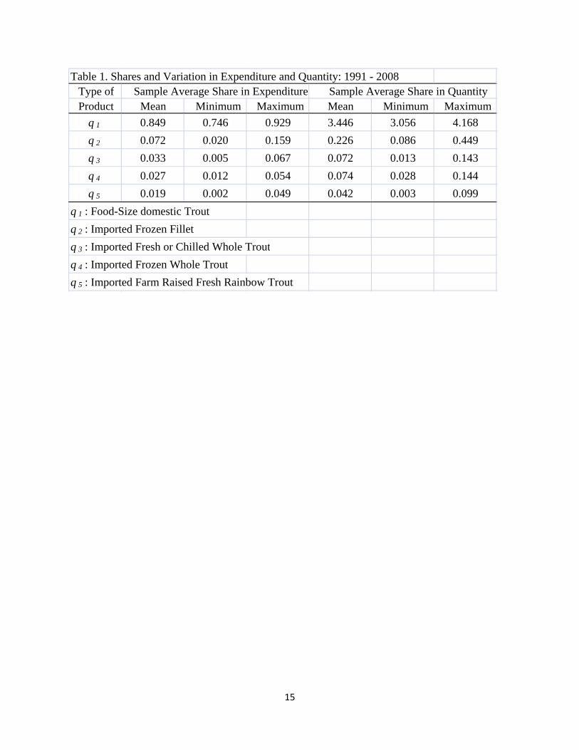
descriptive statistics of normalized budget share and quantity is summarized in Table 1.
[Place Table 1 Approximately Here]
Estimation
As discussed earlier, this study is intended to identify the effects of quantity and currency value
on U.S. domestic trout price. In order to do this, the original LDIAIDS is modified as follows:
(14) ( ) ( )∑ ∑+Δ+Δ=Δj k
kikijiji EQcqcw θlnln ,

9
where kE is the exchange rate between the U.S. dollar and exporting country’s currency, k.
Further, adding up implies the following parametric restrictions:
∑ =i ik 0θ .
In estimation, the adding up of the model causes the contemporaneous covariance matrix of
residuals to be singular. Therefore, one equation was excluded from the system for estimation
purposes. The coefficients of the dropped equation were then calculated from the adding up
restriction. Then, the study added back the dropped equation and deleted another equation and
re-estimated the system in order to determine the parameters and the standard errors of the
former equation. The restricted SUR model, by both symmetry and homogeneity, was used to
estimate quantity and scale elasticity parameters and exchange rate coefficient.
The main motivation for estimating an inverse demand system is that quantities are
assumed to be predetermined naturally. However, fish consumption is assumed to respond to
price incentives, and the actual quantity consumed annually is likely to be influenced by random
perturbations in that year’s price. As a result, the assumption of quantity pre-determinedness
might be questioned. Accordingly, this study tested the pre-determinedness of annual quantities
with the Wu-Hausman test (see Thurman, 1986 and Wu, 1973). The 2χ statistic of the test was
1.25 with 11 degrees of freedom, less than the 10 percent critical value in the chi-square
distribution of 17.2. In sum, the test for the pre-determinedness of quantities could not reject the
null hypothesis, so the restricted SUR estimates reported in Table 2 are supported by this
evidence.
Finally, this study estimates the Allais coefficients to measure the intensity of
substitutable interaction among these five products by using following equations:
(30) ( ) ( )ssjjrriisrrsijijij whwhwhwhwwhwha ////// −+−+−=

10
and
(31) ( )2/ ijiiijij aaa=α ,
where the subscripts r and s refer to some standard pair of goods r and s with which it will be
used to compare the relative strength of substitutability between any other pair, i and j , of
goods. An ijα greater than zero indicates that i and j are more complementary than r and s,
while an ijα less than zero signifies that i and j are stronger substitutes than are r and s. Clearly,
0=ijα means that i and j have the same type of interaction as r and s (Lee and Kennedy, 2008).
Empirical Results
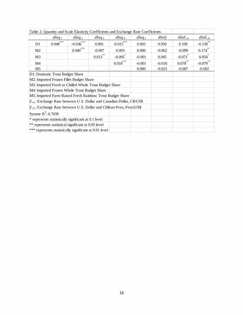
Table 2 summarizes quantity and scale elasticity coefficients estimated by the LDIAIDS
procedure with exchange rate coefficients. The system R2 is 0.70 for the LDIAIDS model.
Thirteen (13) coefficients from the 30 coefficients estimated by the LDIAIDS procedure are
significantly different from zero at least at the 10% level of significance. In particular, four of the
five estimated own quantity elasticity coefficients are significantly different from zero at the 5%
level of significance and two of the three cross quantity elasticity coefficients in the domestic
trout budget equation are significantly different from zero at the 1% level of significance.
However, all five scale quantity elasticity coefficients are not significantly different from zero at
any conventional level.
Related to the exchange rate’s effect on prices, this study found results consistent with
trade theory in the U.S. Dollar - Chilean Peso exchange rate. According to trade theory,
devaluation of an importing country’s currency results in a decrease in the exporting country’s
price and an increase in the importing country’s price. In this study, the exchange rate
coefficients of Chilean currency are estimated as -0.158 for the domestic trout price and 0.174
for imported frozen trout fillets. Both coefficients are statistically significant at 5%. Furthermore,

11
as seen in the previous section, most U.S. imported frozen trout fillets come from Chile. In terms
of these facts, this study calculates the elasticities of exchange rate of Chilean currency on
domestic price and imported frozen trout fillet price in order to quantify the effect of exchange
rate of Chilean currency on domestic trout price and imported frozen trout fillet price (see
Appendix I). According to the calculated elasticities, if the U.S. dollar depreciates 10% in value
relative to the Chilean Peso by, then the U.S. domestic trout price increases by 6.61% and the
imported frozen trout fillet price decreases by 5.84%. Accordingly, results show that a
devaluation of the U.S. dollar against major exporting country currencies supports domestic trout
price.
The quantity and scale elasticity coefficients have been transformed into elasticities using
equations (7.1) through (7.3). Table 3 shows compensated quantity elasticities and scale
elasticities. Compensated quantity elasticities represent the net effect of quantity on price, while
scale elasticities represent the effect of expenditure on price in this system. The results found two
interesting facts. First, the results show that the estimated quantity elasticities are very inelastic
(including both own and cross quantity elasticities). Tomek and Robinson (1990) define the
relationship between quantity and price elasticities as an inverse relationship. Thus, if own
quantity elasticity is less than one in absolute value, demand for own good is elastic. If cross-
quantity elasticity is less than one in absolute value, demand for good j is greatly influenced by a
small change in the price of good i. According to the results, demand for domestic and imported
trout are very elastic because the own quantity elasticities of these five products are very
inelastic. Also, cross price effect on quantity will be greater than one because most of cross
quantity elasticities are very inelastic except for the cross quantity elasticity of domestic trout for

12
imported farm raised fresh whole trout. This result is consistent with those of Barten and
Bettendorf (1989), Park, Thurman, and Easley (2004), and Lee and Kennedy (2008 and 2009).
Second, two goods, i and j, are net quantity complements if 0* >ijf and two goods, i and
j , are net quantity substitutes if 0* <ijf . Contrary to expectation, most cross effects show a net
complementary pattern. In particular, four imported trout products are net complements for
domestic trout. As a result, the low farm price of domestic trout might be due to other reasons
than increased trout imports. One possible reason for this is that with enlargement of the U.S.
seafood market, U.S. seafood consumers prefer other seafood species to trout. This implication
suggests the need for the development for value-added trout products as a means of helping to
strengthen/ensure the economic growth of the domestic trout industry.
Table 4 shows uncompensated quantity elasticities. The uncompensated quantity
elasticity represents the effect of gross quantity on price, which is the sum of net quantity and
scale effect. Therefore, uncompensated inverse demand of a normal good is more quantity elastic
than is compensated inverse demand. As seen in Table 4, own uncompensated quantity
elasticities of domestic trout and imported frozen trout fillets, frozen whole trout, and farm raised
fresh rainbow trout are more elastic than those of the own compensated quantity elasticities. The
own uncompensated quantity elasticity of imported fresh whole trout is less elastic than that of
the own compensated quantity elasticity. Imported frozen trout products including both trout
fillets and whole trout are gross quantity substitutes for domestic trout, while imported fresh
trout products are gross quantity complements for domestic trout.
As seen in Tables 3 and 4, most of the cross effects are complementary rather than
substitutionary, which is inconsistent with the notion that most types of fish are mutual
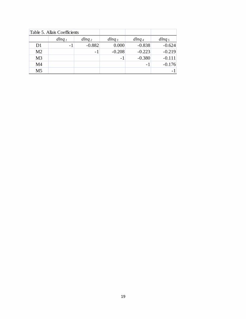
substitutes. Barten and Bettendorf (1989) proposed Allais coefficients as a more adequate

13
measure of commodity interaction. In order to calculate the Allais coefficients, this study
selected domestic trout and imported fresh whole trout as the standard pair of goods r and s,
respectively. This selection causes all other Allais interactions to become negative, implying
stronger substitutes between two commodities i and j than the standard pair of domestic trout, r,
and imported fresh whole trout, s. For example, the Allais coefficient between domestic trout and
imported frozen fillet is -0.882. This result implies that the substitutionary relationship between
domestic trout and imported frozen trout fillets is stronger than is the substitutionary relationship
between domestic trout and imported fresh whole trout. Therefore, by comparing the magnitude
of the coefficients, we can identify the intensity of substitutable interaction between these trout
products. According to the results, the intensity of the substitutable interaction of imported trout
products with domestic trout is ordered as follows: imported frozen trout fillets (-0.882), frozen
whole trout (-0.838), farm raised fresh rainbow trout (-0.624), and fresh whole trout (0.000).
Conclusions
Facing a dynamic change in trout imports, this study tried to identify how imports affect the U.S.
domestic trout industry. In doing so, this study analyzed the quantity effect and exchange rate
effect on domestic trout price using a modified LDI-AIDS model. Over the past two decades, the
nature of trout imports have changed from consisting of primarily frozen trout to fresh or chilled
product. Also, the major exporter into the U.S. market has changed from Argentina to Chile for
frozen products and Canada for fresh trout. According to the results of this study, we found five
important facts related to trout imports during this sample period of time.
First, empirical results show that net effects of imported trout products are
complementary rather than substitutionary for domestic trout. As a result, the low farm price of
domestic trout might be due to other reasons than just increased trout imports. One possible

14
reason is that with enlargement of the U.S. seafood market, U.S. seafood consumers prefer other
seafood species to trout. This implication suggests the need for the development of value-added
trout products that broadly appeal to U.S. seafood consumers’ taste as one means of
strengthening the economic growth of the domestic trout industry.
Second, in light of the relationship between domestic trout price and consumer
expenditure, domestic trout price decreases with an increase in total trout supply into the
domestic market. When we consider imports of frozen trout fillets as a major import product, the
increase in imports of Chilean trout products may have the greatest influence on domestic trout
prices.
Third, imported frozen trout fillets and whole trout are gross-substitutes for domestic
trout, while imported fresh whole trout is a gross-complement to domestic trout. In particular, the
import price of frozen trout is much lower than for those of fresh trout. In 2008, the import prices
of frozen trout fillets and whole trout are $5.29 and $4.19 per kilogram, respectively, while the
import prices of fresh whole trout is $6.24 per kilogram. As a result, increase in low price
imported frozen products are major concerns about domestic trout industry.
Fourth, the estimated Allais coefficients show that own product has strongest
substitutability compared to those of cross products. For domestic trout, the intensity of
substitutable interaction of imported products is frozen trout fillets > frozen whole trout > fresh
whole trout > rainbow trout.
Finally, depreciation of U.S. currency against exporting country’s currency reduces the
negative impact of Chilean imported trout on domestic price.
15
Table 1. Shares and Variation in Expenditure and Quantity: 1991 - 2008Type ofProduct Mean Minimum Maximum Mean Minimum Maximum
q 1 0.849 0.746 0.929 3.446 3.056 4.168q 2 0.072 0.020 0.159 0.226 0.086 0.449q 3 0.033 0.005 0.067 0.072 0.013 0.143q 4 0.027 0.012 0.054 0.074 0.028 0.144q 5 0.019 0.002 0.049 0.042 0.003 0.099
q 1 : Food-Size domestic Troutq 2 : Imported Frozen Fillet q 3 : Imported Fresh or Chilled Whole Troutq 4 : Imported Frozen Whole Troutq 5 : Imported Farm Raised Fresh Rainbow Trout
Sample Average Share in QuantitySample Average Share in Expenditure
16
Table 2. Quantity and Scale Elasticity Coefficients and Exchange Rate Coefficients dlnq 1 dlnq 2 dlnq 3 dlnq 4 dlnq 5 dlnQ dlnE ca dlnE ch
D1 0.048*** -0.036*** 0.001 -0.015*** 0.003 0.050 0.109 -0.158**
M2 0.040*** -0.007 0.003 0.000 -0.062 -0.099 0.174**
M3 0.013** -0.005* -0.001 0.045 -0.071* 0.054*
M4 0.018*** -0.001 -0.018 0.078** -0.079**
M5 0.000 -0.023 -0.007 -0.002D1: Domestic Trout Budget ShareM2: Imported Frozen Fillet Budget ShareM3: Imported Fresh or Chilled Whole Trout Budget ShareM4: Imported Frozen Whole Trout Budget ShareM5: Imported Farm Raised Fresh Rainbow Trout Budget ShareE ca : Exchange Rate between U.S. Dollar and Canadian Dollar, C$/US$E ch : Exchange Rate between U.S. Dollar and Chilean Peso, Peso/US$
Systme R2: 0.7039* represents statistically significant at 0.1 level** represents statistical significant at 0.05 level*** represents statistically significant at 0.01 level

17
Table 3. Compensated Quantity Elasticity and Scale Elasticity dlnq 1 dlnq 2 dlnq 3 dlnq 4 dlnq 5 dlnQ
D1 -0.094 0.029 0.034 0.009 0.022 -0.941M2 0.342 -0.367 -0.068 0.074 0.019 -1.868M3 0.867 -0.149 -0.575 -0.128 -0.015 0.376M4 0.291 0.194 -0.153 -0.312 -0.019 -1.673M5 1.004 0.074 -0.025 -0.028 -0.992 -2.203

18
Table 4. Uncompensated Quantity Elasticity dlnq 1 dlnq 2 dlnq 3 dlnq 4 dlnq 5
D1 -0.894 -0.039 0.003 -0.016 0.005 M2 -1.244 -0.501 -0.130 0.023 -0.016M3 1.187 -0.122 -0.563 -0.118 -0.007M4 -1.129 0.074 -0.208 -0.358 -0.051M5 -0.867 -0.084 -0.097 -0.088 -1.034
19
Table 5. Allais Coefficients dlnq 1 dlnq 2 dlnq 3 dlnq 4 dlnq 5
D1 -1 -0.882 0.000 -0.838 -0.624M2 -1 -0.208 -0.223 -0.219M3 -1 -0.380 -0.111M4 -1 -0.176M5 -1

20
Appendix: Elasticity of Exchange Rate at Mean Elasticity of exchange rate of Chilean currency on domestic price
ch
dd
ch
dd
ch
d
Edpdq
Edqdp
Eddw
lnlnln
'⋅+
⋅= ,
where subscript d and ch represent “domestic” and “Chile”, respectively, and 'p represent the initial price. Since 1=dq at mean and 0=ddq ,
''
158.0lnln ddch
d
ch
d
ch
d
ppE
dEdp
Eddp
Eddw −
=⋅== ,
where 239.0' =dp is average normalized domestic trout price during the sample period of time.
661.0239.0158.0
' −=−
=⋅dch
d
pE
dEdp
Elasticity of exchange rate of Chilean currency on imported frozen fillet price
ch
ff
ch
ff
ch
f
Edpdq
Edqdp
Eddw
lnlnln
'⋅+
⋅= ,
where subscript f represents “imported frozen fillets”. Since 1=fq at mean and 0=fdq ,
''
174.0lnln ffch
f
ch
f
ch
f
ppE
dEdp
Eddp
Eddw
=⋅== ,
where 298.0' =fp is average normalized imported frozen fillet price during the sample period of time.
584.0298.0174.0
' ==⋅fch
f
pE
dEdp

21
Footnote 1. Rates of duty are applied to each HS code. However, since the duty amount of each product is relatively small compared to imported price, this study ignores the duty amount in discussing the imported price. Rates of duty are 5.5¢/kg for HS 0304206005 and 2.2¢/kg for HS 0302110090, 0303210000, and 0302110010. Footnote 2. According to Foltz, Dasgupta, and Devadoss (1999), fresh trout steaks were found to be more popular than frozen trout steaks. Footnote 3. Koo and Kennedy (2005) graphically show that a devaluation in an importer’s currency increases importer’s price and decreases exporter’s price.
22
References Barten, A.P., and L.J. Bettendorf. “Price Formation of Fish: An Application of an Inverse Demand System.” European Economic Review 33(1989): 1509-25. Dasgupta S., J. Foltz, and B. Jacobsen. “Trout Steaks: Consumer Perceptions of a New Food Item.” Journal of Food Distribution Research (November 2000): 38-48. Hanoch, G. “Symmetric Duality and Polar Production Functions.” In Production Economics: A Dual Approach to Theory and Applications, Vol. 1, eds., M. Fuss and D. McFadden, pp. 111-31. Amsterdam: North-Holland, 1978. Kim, H.Y. “Inverse Demand Systems and Welfare Measurement in Quantity Space.” Southern Economic Journal. 63(January 1997): 663-79. Koo W., and P.L. Kennedy. International Trade and Agriculture. Blackwell Publishing, 2005. Lee, Y-J., and P.L. Kennedy. “An Examination of Inverse Demand Models: An Application to the U.S. Crawfish Industry.” Agricultural and Resource Economics Review 37(October 2008): 243-56. Lee, Y-J., and P.L. Kennedy. “An Empirical Investigation on Inter-Products Relationship between U.S. Domestic and Imported Seafood.” Submitted to Journal of Agricultural and Applied Economics, 2009.
Park, H., W.N. Thurman, and J.E. Easley. “Modeling Inverse Demands for Fish: Empirical Welfare Measurement in Gulf and South Atlantic Fisheries.” Marine Resource Economics 19(2004): 331-51. Thurman, W.N. “Endogeneity Testing in a Supply and Demand Framework.” Review of Economics and Statistics 68(1986): 638-46. Tomek, W.G., and K.L. Robinson. Agricultural Product Prices (3rd edition). Ithaca, N.Y.: Cornell University Press, 1990. Weymark, J.A. “Duality Results in Demand Theory.” Eur. Econ. Rev. 14(1980): 377-95. Wu, D.M. “Alternative Tests of Independence Between Stochastic Regressors and Disturbances.” Econometrica 41(1973): 733-50.