Cultural Proximity and Trade∗

Gabriel J. Felbermayr†and Farid Toubal‡

Feb., 2007

Abstract

Cultural proximity may influence bilateral imports through a preference and a trade-

cost channel. In empirical gravity models, conventional measures such as common language

or religion fail to separately identify those channels. We use bilateral score data from the

Eurovision Song Contest, a huge pan-European television show, to construct a measure

of cultural proximity that correlates strongly with conventional indicators. Its statistical

properties allow to identify the trade-cost and preference channels. For trade in differentiated

goods, we find evidence for both channels, with the former accounting for about 65% of the

total effect. There is no preference effect for homogeneous goods.

(JEL Codes: F12, F15, Z10. Keywords: International Trade, Gravity Equation, Cultural

Proximity, Identification.)

∗Thanks to Philippe Aghion, Hartmut Egger, Josef Falkinger, Raquel Fernandez, Wilhelm Kohler, Philippe

Martin, Thierry Mayer, Peter Neary, and Rudolf Winter-Ebmer, and to seminar participants at the universities

of Gottingen and Zurich, WHU-Otto Beisheim School of Management, Paris School of Economics, the 2006

ETSG meeting in Vienna and the 2006 Verein fur Socialpolitik conference in Bayreuth. Part of this research

was undertaken while Felbermayr was visiting Zurich University. Benny Jung and Michael Bohm have provided

excellent research assistance. The usual disclaimer applies.†Department of Economics, University of Tubingen, Nauklerstraße 47, 72074 Tubingen, Germany. Tel.: +49

7071 29 78183. Email: gabriel.felbermayr@uni-tuebingen.de.‡ Universite de Paris I, Pantheon-Sorbonne, CNRS. Centre d’Economie de la Sorbonne, 106-112 Boulevard de

l’Hopital, 75647 Paris. Tel.: +33 (0)1 44 07 83 47. E-mail: toubal@univ-paris1.fr.

1 Introduction

Easy access to foreign markets is an important determinant of bilateral trade volumes and

matters for countries’ per capita income and welfare (Frankel and Romer, 1999; Redding and

Venables, 2004). Usually, researchers model market access as a function of geographical distance.

Cultural proximity has received less attention, although empirical trade flow models typically

include some measures of it (Boisso and Ferrantino, 1997).

Cultural proximity affects bilateral trade flows through preferences (bilateral affinity) and/or

trade costs. Two culturally close countries may trade a lot because they have strong tastes for

each others’ products and/or because trade costs are low. However, only the second channel

relates to market access and has a welfare theoretic interpretation. This paper attempts to dis-

entangle the trade cost channel from the preference channel of cultural proximity in an empirical

bilateral trade flow model.1

Following the recent literature (Anderson and van Wincoop, 2003; Combes, Lafourcade, and

Mayer, 2005), we start with a model of trade in differentiated goods. Our theoretical framework

includes both the preference and the trade cost channels. We exploit information from a yearly

pan-European televised show, the Eurovision Song Contest (ESC). Each participating country

sends an artist to perform a song and grades the other competitors’ performances according

to a strict set of rules. The process gives rise to a matrix of bilateral votes. The grades are

established either by popular juries, or more recently, by televoting.

The ESC data correlates strongly with conventional measures of cultural proximity, such as

common language, religion or ethnicity. Contrary to these measures, the ESC data are both

time-variant and asymmetric. We use this extra variance to identify the preference and the cost

channels separately. In the context of bilateral trade, the slow-moving, symmetric component

of cultural proximity–language, religion, ethnicity–can be associated to conventional transaction

costs. The fluctuating, asymmetric component, in turn, has more to do with preferences.2

Various recent academic papers establish that cultural proximity shapes bilateral ESC scores

(Ginsburgh and Noury, 2004; Ginsburgh, 2005; Clerides and Stengos, 2006). Through their

voting behavior, countries cluster into clubs according to patterns of cultural closeness (Fenn

et al., 2006). Interpreting ESC scores as a measure of cultural proximity poses two empirical

challenges: First, scores need to be purged from the artistic quality of songs. We chose an

1The received literature acknowledges the importance of separately identifying the trade cost and the preference

channels; see Combes, Lafourcade, and Mayer (2005). The study that comes closest in terms of disentangling

different components of the distance coefficient is Huang (2007). However, to our knowledge, to date, there is no

systematic identification exercise related to a widely defined notion of cultural proximity.2Guiso et al. (2006) distinguish between inherited and fast-moving aspects of culture; see also Manski (2000).

1

agnostic strategy and use song-specific fixed effects. Second, ESC rules imply that countries

cannot establish complete rankings of their competitors’ performances. We address the resulting

measurement bias by a two-step Heckman procedure.

Recent economic literature defines culture as a set of “customary beliefs and values that

ethnic, religious, and social groups transmit fairly unchanged from generation to generation”

(Guiso, Sapienza, and Zingales, 2006). That research puts much effort into establishing a causal

link between culture and economics, see Spolaore and Wacziarg (2006) or Giuliano, Spilimbergo,

and Tonon (2006). Common instruments or proxies for the concepts of beliefs and values are

common language, history, religion, ethnicity or genetic traits.

In the trade literature, authors tend to use the above list of proxies as measures of cultural

proximity without always analyzing the fundamental link to beliefs and values.3 For example,

Rauch and Trindade (2002) and Combes, Lafourcade, and Mayer (2005) emphasize the impor-

tance of ethnic ties across countries or regions for the flow of information and hence for bilateral

trade. There is also a growing literature that correlates attitudes, sentiments, or customary

beliefs to the magnitude of bilateral trade (Disdier and Mayer, 2005; Guiso, Sapienza, and Zin-

gales, 2004). The existing studies use instrumental variable techniques and find little evidence

for reverse causality. Exploiting the time series nature of our data, we confirm this result but

focus squarely on hitherto unresolved identification problems.

We view cultural proximity as the degree of affinity, sympathy, or even solidarity, between

two countries. It is driven by the feeling of sharing a common identity and of belonging to the

same group. In the sociological literature (Straubhaar, 2002), there is no doubt that cultural

proximity can be asymmetric or fluctuate over time. A country can command huge respect and

sympathy for its cultural, societal, and technological achievements without this feeling being

reciprocal. For example, the ESC score data suggests that France has been relatively popular in

Europe during the sixties and seventies, without these feelings being reciprocal. However, the

relative attraction of France has declined since then.

We frame our analysis in a monopolistic competition trade model close to Hanson and

Xiang (2004). However, in the specification of the utility function, we allow for an origin-

specific preference term (Combes, Lafourcade and Mayer, 2005). That setup allows to study the

trade cost and preference channels of cultural proximity for aggregates of goods with different

degrees of differentiation. We propose and implement two alternative identification strategies.

3Most cross-sectional gravity equations use time-invariant, symmetric measures of cultural proximity, e.g., a

dummy for common language, or for colonial ties. Recent examples include Alesina and Dollar (2004), who have

used cultural proximity measures in the context of explaining international aid, and Rose (2004), who studies the

effect of WTO membership on trade. Melitz (2002) and Hutchinson (2006) provide thorough discussions of the

empirical relation between language and bilateral trade.

2

In the first, we assume that only the time-invariant elements of cultural proximity matter for

trade costs. In the second, we assume that trade costs are symmetric, i.e., they affect exports

and imports of a country from or to some trade partner in the same way. We discuss these

assumptions and find them largely in line with arguments presented in the theoretical and

empirical literature.

Econometrically, we follow Baldagi, Egger, and Pfaffermayr (2003) and include full sets of

interaction terms of importer/exporter dummies with year fixed effects into our regressions.

This strategy is a natural extension of the fixed effects approach discussed by Feenstra (2004)

and used in Redding and Venables (2004) to a framework with time-varying variables. It appro-

priately controls for multilateral resistance (Anderson and van Wincoop, 2003) and other sorts

of unobserved country-specific heterogeneity.4 We deal with the potential endogeneity of the

time-variant, and/or asymmetric components of cultural proximity by means of instrumental

variables techniques and by using dyadic fixed effects.

Our main empirical results can be summarized as follows. First, quality-adjusted ESC scores

are good summary proxies of cultural proximity. They correlate strongly with conventional mea-

sures of cultural proximity such as linguistic, genetic, religious, and legal system proximity and

yield comparable overall predictions in empirical gravity equations. In line with expectations,

the total cultural proximity effect is by an order of magnitude larger for differentiated goods than

for homogeneous goods. Second, we use the adjusted ESC scores in two alternative econometric

specifications that allow to disentangle the preferences and the trade-costs effects. With aggre-

gate bilateral imports, the total effect of moving from the lowest to the highest possible degree

of cultural proximity leads to trade creation of about 150%. Assuming that only time-invariant

components of cultural proximity are relevant for the trade-cost channel, the preference effect

accounts for about 50% of total trade creation, the remaining 100% made up by the cost channel.

Focusing on differentiated goods (according to Rauch, 1999), overall trade creation is slightly

smaller (due to the smaller elasticity of substitution), but the preference channel again makes

up about a third of the total effect. Assuming that only symmetric components of cultural

proximity are relevant for the trade-cost channel, we find no evidence for a preference effect in

aggregate trade. However, focusing on differentiated goods, we detect a significant preference

channel, which amounts to about half of total trade creation. We conclude that a significant

fraction of the total trade-creating effect of cultural proximity works through the preference

channel.

The remainder of this paper is structured as follows. In Section 2, we provide a thorough

discussion of the data. In section 3, we propose a theoretical framework and discuss the empirical

4Baier and Bergstrand (2006) interact country and year fixed effects, too.

3

strategy. In section 4, we present the main results and provide some robustness checks. In Section

5, we conclude.

2 Eurovision Song Contest score data

In this section, we discuss our data and show that the ESC scores are meaningful measure of

cultural proximity. We also discuss their statistical properties.

2.1 The setup of the contest

In 1955, a couple of European broadcasting stations represented in the European Broadcasting

Union (EBU) founded the Eurovision Song Contest (ESC). A year later, the first contest took

place in Lugano, Switzerland. The idea of the ESC is that each participating country selects an

artist or a group of artists to perform a song, which is then graded by the other countries.

We focus on the period 1975-2003, in which the described grading rules have been stable.5

On average, from 1975 to 2003, 21.6 countries participated in the ESC, with the minimum par-

ticipation being at 18 countries. Contest participants are mostly European countries. However,

Israel participates on a regular basis and Morocco has participated once. Each ESC is broadcast

by television, and since 1985, this happens via satellite. In 2005, the contest was broadcast live

in over 40 countries to over 100 million spectators. Until 1988, the scores were decided upon by

a jury that is not necessarily consisting of experts. Nowadays, the scores are national averages

obtained through a televoting process with huge popular participation.

Since 1975, each country scores the other countries’ performances on a scale from 0 to 12.

The scores 9 and 11 are not allowed and 12 is the highest possible score. Each of the ten strictly

positive grades has to be allocated exactly once; remaining countries are graded zero. The

winner is the country that collects the largest sum of points.

2.2 Measurement issues

We argue that ESC scores are appropriate summary indicators of cultural proximity. However,

this interpretation poses two difficulties. First, the scores may also reflect the quality of the

song. Second, the rules of the contest disallow ties for the ten most popular songs and force ties

for the least popular ones.

Denote by Sijt country i′s support of country j′s performance at time t. Let Sijt depend

positively on the quality of the song, Qjt, on the degree of country i′s feeling of cultural proximity

5Until 2003, the last year in our sample, the contest was organized in a single round. From 2004 onwards,

there are two rounds to accommodate the rising number of participants.

4

towards j at time t, Πijt, and on noise, uijt, i.e.,

Sijt = S (Πijt, Qjt, uijt) . (1)

We do not model the aggregation of jury members’ or telespectators’ preferences into Sijt.

However, we need to be more explicit on the mapping of Sijt into actual scores, denoted by

ESCijt. This mapping is shaped by the official rules of the competition.

Assume that at time t, Nt ≥ 11 countries participate in the competition. Each country grades

the other countries’ performances; hence, for each i 6= j and t, there are Nt − 1 realizations of

Sijt. According to ESC rules, each country must award strictly positive points to 10 songs,

the remaining Nt − 11 songs receive zero points. Assuming that each country i ranks the

competitors’ performances according to the realization of Sijt, we can introduce a function

G (Sijt) : R+ → {0, 1, 2, 3, 4, 5, 6, 7, 8, 10, 12} which maps support Sijt into scores. G (.) is a

positive, monotonic, increasing function under the restriction that each non-zero score has to be

used exactly once. That rule implies that it is impossible to express indifference between high-

ranked alternatives. More importantly, the observer cannot infer anything about the ranking

of the Nt − 11 lowest-ranked alternatives, except that they are weakly inferior to the 10th best

song. We can therefore write

ESCijt =

G (Sijt) > 0 if Sijt ≥ Sit

0 if Sijt < Sit

, (2)

where Sit is the threshold support below which country i awards zero points.

ESC scores are only partly informative about cultural proximity if ESCijt = 0. For those

observations, there is a negative correlation between measurement error and the true amount of

cultural proximity, which would bias estimates in a way that is difficult to correct for. Hence,

we use only observations for which ESCijt > 0 and implement a Heckman (1979) two-stage

correction procedure to deal with the resulting non-random sample composition.6 In the first

stage, we formalize the probability that country i receives a strictly positive rating by country

j as a Probit model,

Pr(Sijt ≥ Sit

)= Φ

(χ0 ln Πij + χ1 ln Qjt

), (3)

where Φ is the c.d.f. of the standard normal distribution, and equation (1) has been linearized.

We estimate the model using observable proxies of cultural proximity that are available for all

country pairs Πij : common language, common religion and common legal origin. We control for

song quality capturing Qjt by a comprehensive set of song-specific fixed effects.

6Qualitatively, our results do not hinge on that correction.

5

We use the Probit equation to compute the inverse Mill’s ratio λijt ≡ λ(Πij , Qjt

)that we

then include into our gravity regressions.7 λ measures the hazard of selection into the model; in

our case, whether a performance with quality Qjt of a country with cultural proximity Πijt will

be awarded a strictly positive score from country i. Countries do not participate permanently

in the ESC, so we have checked whether selection into participation is random. It does not turn

out that past success systematically determines the probability to stand at the contest. Hence,

we do not further pursue this potential selection issue.

To make use of the ESC measure in our gravity equations, for ESCijt > 0, we linearize (2)

so that ESCijt = ln Πijt + χ ln Qjt + ξλijt + uijt from where we compute a measure of cultural

proximity

lnΠijt = ESCijt − χ lnQjt − ξλijt − uijt. (4)

As in the Probit equation, we account for unobserved song quality by including a set of song-

specific fixed effects. Since we interpret the ordinal ESC score data in a cardinal way, in all

our calculations we enforce an even spacing of scores.8 Moreover, to facilitate comparison with

conventional measures of cultural proximity, we rescale the data so that ESCijt ∈ (0, 1).9

2.3 ESC scores as summary indicators of cultural proximity

ESC data has been used in academic research, albeit not in trade empirics. Recently, Ginsburgh

(2005) shows that conventional measures of cultural proximity determine ESC outcomes to

a large extent, refuting the alternative hypothesis of vote trading (logrolling). Clerides and

Stengos (2006) and Spierdijk and Vellekoop (2006) similarly document the importance of culture

for scoring outcomes. Haan, Dijkstra, and Dijkstra (2005) test whether the transition of the

grading process from jury-based voting to generalized televoting has strengthened the role of

cultural proximity and answer this question in the affirmative. Fenn et al. (2006) run a cluster

analysis and find evidence for unofficial cliques of countries along lines of cultural proximity.

Table 1 shows pairwise correlation coefficients between quality-adjusted ESC scores and

conventional measures and reports the P-values for the null-hypothesis that the correlation co-

efficient is zero. The quality adjusted ESC scores are the residuals from a regression of raw scores

on song-dummies. We consider the following time-invariant and symmetric measures of cultural

proximity used in the literature: (i) a common language dummy; (ii) the continuous Dyen et al.

(2002) measure of linguistic proximity; (iii) a dummy for common legal origin borrowed from

7The inverse Mill’s ratio is given by φ“χ0 ln Πij + χ1Qjt

”/ Φ

“χ0 ln Πij + χ1Qjt

”.

8We use the ESC score as a cardinal expression of Sijt, while the scores really reflect ordinal preference

rankings. This practice may introduce attenuation bias due to additional measurement error.9First, the original score of 10 is set to 9 and the score 12 is set to 10. Then, we divide all scores by 10.

6

La Porta et al. (1999); (iv) a continuous religious proximity measure based on Alesina et al.

(2003)10; (v) a measure of ethnic links based on the stock of individuals born in country i but

residing in country j; (vi) a measure of genetic similarity used by Giuliano, Spilimbergo, and

Tonon (2006) or Spolaore and Wacziarg (2006). To capture geographical proximity, we use an

adjacency dummy and geographical distance between main cities (in kilometers). Appendix A

provides information on the summary statistics of the variables, their exact definition and the

data sources.

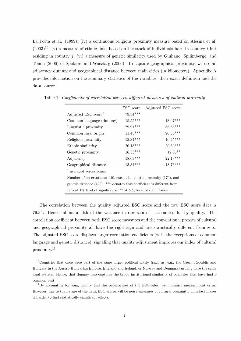
Table 1: Coefficients of correlation between different measures of cultural proximity

ESC score Adjusted ESC score

Adjusted ESC score1 79.34***

Common language (dummy) 15.55*** 13.67***

Linguistic proximity 29.91*** 38.66***

Common legal origin 11.45*** 20.33***

Religious proximity 13.34*** 16.45***

Ethnic similarity 20.18*** 20.63***

Genetic proximity 16.33*** 12.05**

Adjacency 18.63*** 22.13***

Geographical distance -13.81*** -18.76***1 averaged across years.

Number of observations: 940, except Linguistic proximity (176), and

genetic distance (422). *** denotes that coefficient is different from

zero at 1% level of significance, ** at 5 % level of significance.

The correlation between the quality adjusted ESC score and the raw ESC score data is

79.34. Hence, about a fifth of the variance in raw scores is accounted for by quality. The

correlation coefficient between both ESC score measures and the conventional proxies of cultural

and geographical proximity all have the right sign and are statistically different from zero.

The adjusted ESC score displays larger correlation coefficients (with the exceptions of common

language and genetic distance), signaling that quality adjustment improves our index of cultural

proximity.11

10Countries that once were part of the same larger political entity (such as, e.g., the Czech Republic and

Hungary in the Austro-Hungarian Empire, England and Ireland, or Norway and Denmark) usually have the same

legal system. Hence, that dummy also captures the broad institutional similarity of countries that have had a

common past.11By accounting for song quality and the peculiarities of the ESC-rules, we minimize measurement error.

However, due to the nature of the data, ESC scores will be noisy measures of cultural proximity. This fact makes

it harder to find statistically significant effects.

7

2.4 Properties of ESC scores

In this subsection, we briefly discuss two important statistical properties of the ESC scores.

First, they exhibit some reciprocity, but they are far from symmetric. Second, they exhibit

meaningful time variation.

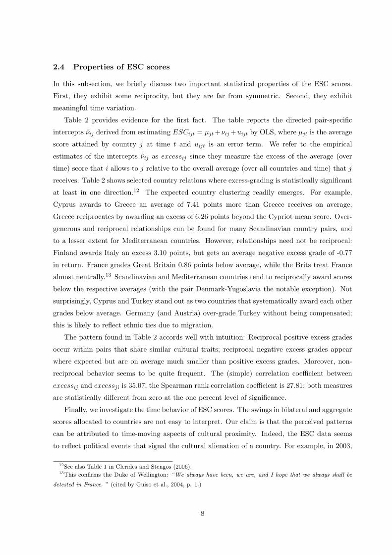
Table 2 provides evidence for the first fact. The table reports the directed pair-specific

intercepts νij derived from estimating ESCijt = µjt +νij +uijt by OLS, where µjt is the average

score attained by country j at time t and uijt is an error term. We refer to the empirical

estimates of the intercepts νij as excessij since they measure the excess of the average (over

time) score that i allows to j relative to the overall average (over all countries and time) that j

receives. Table 2 shows selected country relations where excess-grading is statistically significant

at least in one direction.12 The expected country clustering readily emerges. For example,

Cyprus awards to Greece an average of 7.41 points more than Greece receives on average;

Greece reciprocates by awarding an excess of 6.26 points beyond the Cypriot mean score. Over-

generous and reciprocal relationships can be found for many Scandinavian country pairs, and

to a lesser extent for Mediterranean countries. However, relationships need not be reciprocal:

Finland awards Italy an excess 3.10 points, but gets an average negative excess grade of -0.77

in return. France grades Great Britain 0.86 points below average, while the Brits treat France

almost neutrally.13 Scandinavian and Mediterranean countries tend to reciprocally award scores

below the respective averages (with the pair Denmark-Yugoslavia the notable exception). Not

surprisingly, Cyprus and Turkey stand out as two countries that systematically award each other

grades below average. Germany (and Austria) over-grade Turkey without being compensated;

this is likely to reflect ethnic ties due to migration.

The pattern found in Table 2 accords well with intuition: Reciprocal positive excess grades

occur within pairs that share similar cultural traits; reciprocal negative excess grades appear

where expected but are on average much smaller than positive excess grades. Moreover, non-

reciprocal behavior seems to be quite frequent. The (simple) correlation coefficient between

excessij and excessji is 35.07, the Spearman rank correlation coefficient is 27.81; both measures

are statistically different from zero at the one percent level of significance.

Finally, we investigate the time behavior of ESC scores. The swings in bilateral and aggregate

scores allocated to countries are not easy to interpret. Our claim is that the perceived patterns

can be attributed to time-moving aspects of cultural proximity. Indeed, the ESC data seems

to reflect political events that signal the cultural alienation of a country. For example, in 2003,

12See also Table 1 in Clerides and Stengos (2006).13This confirms the Duke of Wellington: “We always have been, we are, and I hope that we always shall be

detested in France. ” (cited by Guiso et al., 2004, p. 1.)

8

Table 2: ESC scores: Selected deviations from means

Country i Country j excessij std. err. excessji std. err.CYP GRC 7.41 0.65 6.26 0.65ITA PRT 3.95 0.63 0.02 0.63DNK ISL 3.27 0.72 2.05 0.72FIN ITA 3.10 0.65 -0.77 0.65DNK SWE 2.99 0.55 1.98 0.55ISL SWE 2.95 0.65 1.56 0.65ESP ITA 2.95 0.63 1.70 0.63CYP YUG 2.67 0.82 2.49 0.82HRV MLT 2.52 0.78 3.17 0.78TUR YUG 2.22 0.75 3.21 0.75DNK NOR 2.04 0.57 0.79 0.57GER TUR 1.79 0.53 -0.70 0.53CYP ESP 1.79 0.57 -0.27 0.57ESP GRC 1.77 0.54 2.62 0.54ISL NOR 1.71 0.65 1.08 0.65NOR SWE 1.56 0.50 2.64 0.50BEL NLD 1.33 0.55 0.30 0.55AUT TUR 1.12 0.55 -0.21 0.55FIN SWE 1.06 0.54 0.67 0.54FRA GBR -0.86 0.49 0.18 0.49ESP NOR -1.01 0.49 -1.37 0.49ESP SWE -1.39 0.49 -1.20 0.49ITA SWE -1.51 0.65 -0.93 0.65DNK ESP -1.66 0.55 -0.39 0.55ISR ITA -1.73 0.69 -1.73 0.69HRV SWE -1.76 0.78 -3.06 0.78DNK HRV -1.92 0.98 -2.53 0.98CYP TUR -2.09 0.58 -1.22 0.58DNK YUG -2.17 0.78 1.34 0.78Pair-specific intercepts, means adjusted. All estimates are significant atthe 10 percent level. All country pairs in the table occur at least 10 times in thedata. Excessij denotes the score awarded by i to j in excess to j’s average score.

the UK was punished by European voters for her support of the war in Iraq. In that year,

its total score was zero, which is a rare event given the numerics of the ESC rules. Similarly,

when Austrians elected Kurt Waldheim, a person with an unclear record during World War

II, as president, aggregate scores touched zero, too. Other examples are readily found. While

the examples cited above mark short-term effects, the data also reveals long-run trends. For

example, the popularity of countries seems subject to cycles that are difficult to reconcile with

underlying movements in musical quality. For example, France scored high in the seventies,

when France was seen as an example to follow and la Chanson Francaise enjoyed Europe-wide

popularity. Since then, this popularity has faded; actually, it seems that France now suffers

the drawbacks from its “exception culturelle”. The example of Italy offers a similar, but less

spectacular, picture. It is well possible that the popularity of celtic culture (Ireland) will suffer

the same fate.14

14In the Appendix, we present the time profile of multilateral unadjusted ESC scores earned by frequently

9

3 Theoretical framework and empirical setup

3.1 Cultural proximity in the gravity model

We base our theoretical model on the multi-country monopolistic competition model of trade

(see Feenstra, 2004, for an overview). Each country i is populated by a representative individual

who derives utility from consuming varieties produced in different sectors, s = 1, ..., S, and

possibly originating from different countries, j = 1, ..., C. Following Hanson and Xiang (2004),

we assume a two-tier demand system. Consumers have identical Cobb-Douglas preferences, with

θs the share of consumption spending on sector s and∑

s θs = 1. For each sector s, a continuum

of varieties from different countries is aggregated using a standard CES utility function. We

denote by z the index of a generic variety, by nsjt the number of sector-s varieties produced

in country j at time t and σs > 1 the sectoral elasticity of substitution between varieties. The

quantity of consumption in country i of variety z from country j and sector s is misjt (z).

Moreover, as Combes, Lafourcade, and Mayer (2005), we allow for a specific weight aisjt ≥ 0

to describe the special preference of the representative consumer in country i for goods from

country j. Hence, the utility function is given by

Uit =∑

s

θs ln

C∑

j=1

∫

nsjt

[aisjtmisjt (z)]σs−1

σs dz

. (5)

This representation allows to consider groups of varieties (‘sectors’) with different degrees of

within-group substitutability.

We assume that all varieties from the same origin bear the same f.o.b. (ex factory) price

psjt (reflecting symmetric production technologies within sectors), and that iceberg ad-valorem

trade costs payable for deliveries from j to i, tisjt ≥ 1, do not depend on the characteristics of

the varieties within a sector. Hence, the c.i.f. price paid by consumers pisjt = psjttisjt is the

same for all varieties imported from j. It follows that consumed quantities misjt are identical

for all z.

Maximizing (5) subject to an appropriate budget constraint, one derives country i′s demand

quantity misjt for a generic variety. Calculating the c.i.f. value of total sector-s imports from

country j at time t as Misjt = nsjtpisjtmisjt, we find

Misjt =(

aisjt

tisjt

)σs−1

φistφjst. (6)

We follow Redding and Venables (2004) and define φist ≡ θsEitPσs−1ist as country i′s market

capacity for sector-s varieties, and φjst ≡ nsjtp1−σssjt as the sector-s supply capacity of the ex-

participating countries. Many of the swings in scores can be recognized as coinciding with important political or

societal events. A detailed analysis, is, however, beyond the scope of the present paper.

10

porting country j. Pist is the sectoral price index, Pist =[∑C

j=1

(aisjt

tisjt

)σs−1p1−σs

sjt nsjt

] 11−σ

and

Eit denotes country i′s GDP.

We do not close the model by explicitly specifying supply side and equilibrium conditions,

since this is not needed for our empirical investigation. However, we need to clarify the role of

cultural proximity in shaping bilateral trade flows. Cultural proximity affects the bilateral trade

equation (6) in two ways. On the one hand, it lowers direct trade costs, tisjt : Costly translation

and cultural advisory services are redundant when partners share a common language or/and

interpret non-verbal communication correctly. Contracting costs are lower when buyers and

sellers operate in similar legal environments, and trust builds up faster when there are ethnic

links. Moreover, cultural proximity indirectly affects trade costs as it facilitates the formation of

business and/or social networks. In turn, these networks help to overcome informational trade

barriers (Rauch and Trindade, 2002). We refer to this channel as to the trade cost channel of

cultural proximity.

On the other hand, cultural proximity is also reflected in the bilateral affinity parameter

aisjt. A high value of aisjt means that the representative consumer in country i puts a high

value on products produced in country j. Equation 6 together with the assumption σs > 1

implies that this situation leads to larger sectoral trade volumes. We dub this second channel

the preference channel of cultural proximity.

We now specify how country i′s cultural proximity to country j is related to bilateral affinity

and trade costs. In both cases, we allow for this link to depend on sectoral characteristics: in

particular, it is plausible that the preference channel is weaker in trade of homogeneous goods.

We assume that country i′s preference for goods from j, aijt, depends on Πijt in the following

way:

ln aisjt = αs lnΠijt. (7)

Concerning trade costs tisjt, we assume that they are driven by three factors:15 (i) Transport

costs Kijt = It · DIST δsij · eγs(1−ADJij), where DISTij refers to geographical distance DISTij ,

ADJij is a dummy that takes value of unity if two countries share a common border, and It

captures the general state of transport technology. (ii) Trade policy Tijt = Tt · eϕs(1−FTAijt),

where FTAijt takes the value of one if both countries are in the same free trade agreement.16

(iii) Cultural proximity Πijt. All parameters are defined as positive numbers. For the sake of

simplicity (and in line with the literature), we assume a log-linear relationship between tisjt and

15See Anderson and van Wincoop (2004) for a classification of different types of trade costs.16We have tried to use direct measures of trade policy, i.e., average tariff rates. This leads to a number of

conceptual difficulties, but leaves our main empirical results unchanged.

11

its determinants

tisjt = K · It ·DIST δsij · eγs(1−ADJij) · Tt · eϕs(1−FTAijt) ·Π−βs

ijt , (8)

where K is a constant. We expect that the trade cost elasticity of cultural proximity, βs is

smaller for homogeneous goods than for differentiated goods.

3.2 Two alternative identification strategies

We can now substitute expressions (4), (8) and (7) into the gravity equation (6). We neither

observe song quality Qjt nor the sectoral market and supply capacity terms φist and φjst. We

control for these variables by using a comprehensive set of interaction terms of exporter and

importer fixed effects with year fixed effects and estimate baseline gravity equations sector by

sector :

ln Misjt = η0sESCijt − δs lnDISTij + γsADJij + ϕ0

sFTAijt (9)

+ξ0sλijt + νs + νst + νist + νjst + εisjt,

where η0s ≡ (σs − 1) (αs + βs), δs ≡ δs (σs − 1), γs ≡ γs (σs − 1), ξ0

s ≡ ξs (σs − 1), and ϕ0s ≡

(σs − 1)ϕs. The term νs is a constant, νst is a set of year dummies, νist is a comprehensive

set of importer × year fixed effects that control for the demand capacity φist and νjst collects

exporter × year fixed effects to control for the supply capacity φsjt and song quality Qjt. Finally,

εisjt ≡ η0suisjt is the error term. This strategy makes the inclusion of GDP or price data

redundant. It also frees us from the need to think about the choice of proper deflators for right

and left-hand side variables of the gravity equation.17

Specification (9) can be estimated sector by sector using available data. The total effect

of cultural proximity can then be identified using some external information on the value of

σs, e.g. by drawing on table 7 in Anderson and van Wincoop (2004). However, we do not

need information on σs to assess the relative importance of the trade-cost versus the preference

channels for given s. In the remainder of this section we discuss two strategies to identify αs

and βs separately.18

In contrast to conventional measures of cultural proximity, quality-adjusted ESC scores are

not necessarily reciprocal. And they are time-variant. This additional variance provides us with

17Baldagi, Egger, and Pfaffermayr (2003) first propose the use of interaction terms between country and time

fixed effects in econometric gravity models, without, however, offering a theoretical rationale. The latter follows

immediately from Anderson and van Wincoop (2003). Baier and Bergstrand (2006) use a similar strategy in their

work on the effects of free trade agreements.18Absent endogeneity concerns (which we address in subsection 3.3), our empirical strategy allows consistent

estimation of average effects; since changes in cultural proximity affect multilateral resistance terms (price indices)

differently, the true coefficient is not constant across countries (Anderson and van Wincoop, 2003).

12

two natural identification strategies. These strategies build on a decomposition of country i′s

cultural proximity to country j (Πijt) into three components,

Πijt = πij πijtπijt, (10)

where, for the sake of simplicity, we postulate a multiplicative relationship. The first component

πij is time-invariant, but potentially asymmetric; the second is symmetric (i.e., πijt = πjit), but

potentially time-variant, while the third is both potentially asymmetric and time-variant.

In our first approach, we make the following assumption:

Assumption 1. Trade costs depend on cultural proximity only through the time-invariant

component πij .

The motivation for this assumption is that the costs of doing business between two countries

depend on linguistic, religious, or ethnic ties, which, if at all, change very slowly over time. To

the extent that Assumption 1 holds true, one can unambiguously attribute the time variant

component of cultural proximity, πijtπijt, to the preference channel. To filter out time-invariant

components, we estimate for each sector s the following ‘dyadic fixed effects gravity’ (DFEG)

model:

lnMisjt = η1sESCijt − ϕ1

sFTAijt + ξ1sλijt + νs + νst + νist + νsjt + νsij + εsijt, (11)

where νsij denotes the comprehensive set of country-pair specific fixed effects. Running (11)

for each sector s (and for aggregate data) we get first estimates of the preference channel α1s =

η1s/ (σs − 1) and of the trade-costs channel as β1

s =(η0

s − η1s

)/ (σs − 1) .

The parameter η1 is identified by drawing on time-variance in cultural proximity, which

reflects fashions and fads and is therefore attributable to the preference channel. Note that we

do not assume that the preference channel is driven exclusively by time-variant components of

cultural proximity. Of course, we can use (11) also on aggregate data, since sectoral differences

enter only through potentially different parameter values.

There is a natural way of validating our identification strategy. Country i’s imports from

j depend on the time variant component of cultural proximity πijtπijt through the preference

channel. However, country i’s exports to j should depend on πijtπijt only to the extent that

cultural proximity is actually symmetric. We have seen in Table 2 that this is not systematically

the case. Hence, we expect that Πijt affects imports more strongly than exports.

Assumption 1 would be violated if the trade-cost related component of cultural proximity

changed over time. We do not expect large shifts to occur in the time span and country sample

that we study (1975-2003, European countries). However, linguistic, ethnic or religious proximity

between countries can change, for example due to migration or due to learning (which might

13

well be driven by trade itself; see below for more discussion). Then, η1s based on (11) may

be a biased estimate of the preference channel, as part of the time change in Πijt also affects

the cost channel. Regardless of the trend in time-variant component of cultural proximity, we

would expect η1s to overestimate the true effect (σs − 1)αs. In the extreme case, where the

time-variance of the trade-cost relevant component of cultural proximity cannot be restricted,

we would actually estimate η1s = (σs − 1) (αs + βs).

We therefore work with a second strategy, which builds on the following assumption:

Assumption 2. Trade costs are symmetric (but may be time-variant). I.e., tsijt = tsjit. This

is equivalent to stating that trade costs depend only on cultural proximity through the symmetric

component πijt.

The prime motivation behind Assumption 2 is its wide-spread use in theoretical work. It im-

plies that a decrease in trade costs through an increase in cultural proximity does not have a

systematically different effect on imports and exports of a country. Under Assumption 2, and

using equation (6) we can write country i′s exports to j relative to its imports from j (both

measured c.i.f.)Msijt

Msjit=

(asijt

asjit

)σ−1

φsitφsjt (12)

where now φsit ≡ nsit (psitPsit)1−σs /Esit and φsjt ≡ Esjt (psjtPsjt)

σs−1 /nsjt. Note that in deriv-

ing (6) we have not assumed that bilateral trade positions are balanced. Even if both countries

share the same values for nsit, psit, Psit, and Esit, and trade costs are symmetric, tsijt = tsjit, due

to the asymmetric preference term, bilateral trade positions need not be balanced, so that the

ratio Msijt/Msjit is not necessarily equal to unity. This argument holds also on the aggregate

level.19 The summary statistics in the Appendix show that bilateral trade positions display a

large degree of variation across country pairs and time. Similarly, quality-adjusted measures of

cultural proximity display asymmetry and time variation.

Substituting ln ajit = α lnΠijt into (12) and using equation (4), we obtain the following

empirical specification that we dub ‘bilateral trade balance equation’.

ln Msijt − ln Msjit = η2s (ESCijt −ESCjit) + ξ2

s (λijt − λjit) + νsit + νsjt + εsijt, (13)

where η2s ≡ (σs − 1)αs, ξ2

s ≡ (σs − 1) ξs. The vectors νsit and νsjt collect interactions between

country and year fixed effects which control for the difference of country i’s and j’s supply and

19Davis and Weinstein (2002) derive a bilateral trade balances model that holds for any trade model that implies

perfect specialization. They discuss the possibility of bilateral trade imbalances. If supply and demand conditions

are not symmetric across two countries–as in our case due to the bilateral preference term in the description of

utility–bilateral trade positions need not be zero. Aggregate balance is then restored by triangular trade.

14

demand capacities. Indirectly, those fixed effects also account for the real bilateral exchange

rate, as they summarize the underlying stances of monetary and fiscal policy in both countries.

Again, we compute the size of the preference channel as α2s = η2

s/ (σs − 1) and the size

of the trade-costs channel as β2s = (η0

s − η2s)/ (σs − 1) . We can run model (13) separately for

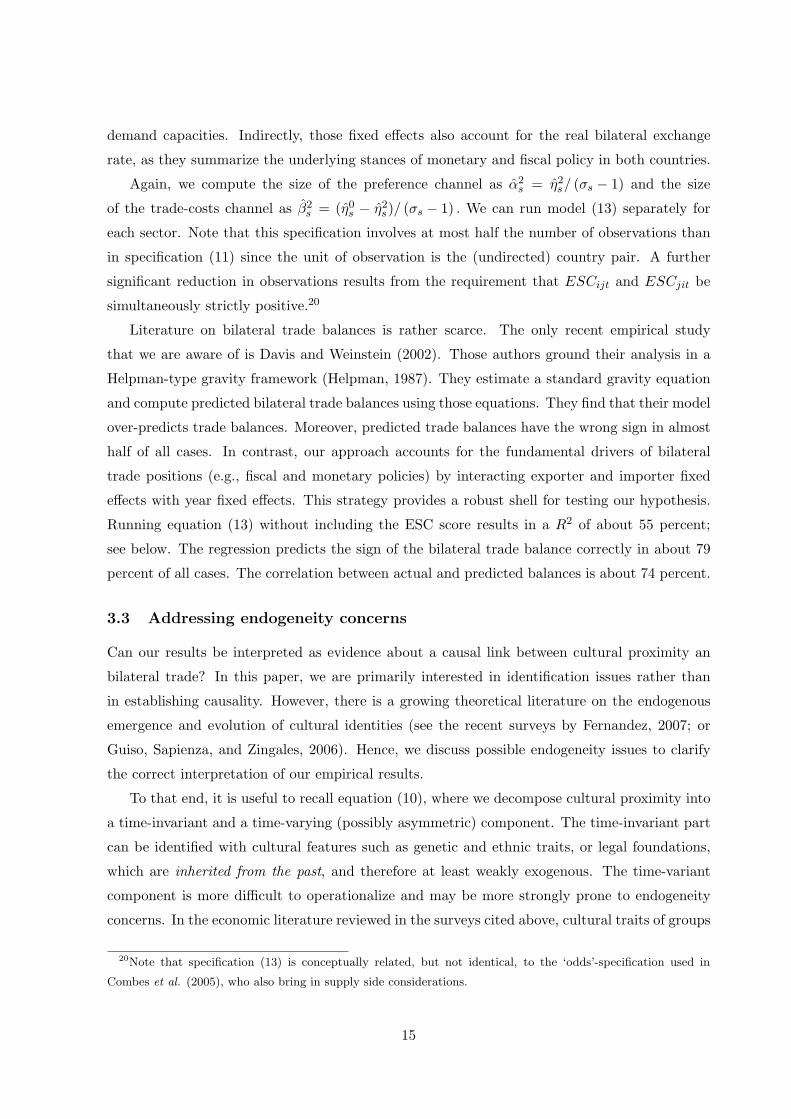
each sector. Note that this specification involves at most half the number of observations than

in specification (11) since the unit of observation is the (undirected) country pair. A further

significant reduction in observations results from the requirement that ESCijt and ESCjit be

simultaneously strictly positive.20

Literature on bilateral trade balances is rather scarce. The only recent empirical study

that we are aware of is Davis and Weinstein (2002). Those authors ground their analysis in a

Helpman-type gravity framework (Helpman, 1987). They estimate a standard gravity equation

and compute predicted bilateral trade balances using those equations. They find that their model

over-predicts trade balances. Moreover, predicted trade balances have the wrong sign in almost

half of all cases. In contrast, our approach accounts for the fundamental drivers of bilateral

trade positions (e.g., fiscal and monetary policies) by interacting exporter and importer fixed

effects with year fixed effects. This strategy provides a robust shell for testing our hypothesis.

Running equation (13) without including the ESC score results in a R2 of about 55 percent;

see below. The regression predicts the sign of the bilateral trade balance correctly in about 79

percent of all cases. The correlation between actual and predicted balances is about 74 percent.

3.3 Addressing endogeneity concerns

Can our results be interpreted as evidence about a causal link between cultural proximity an

bilateral trade? In this paper, we are primarily interested in identification issues rather than

in establishing causality. However, there is a growing theoretical literature on the endogenous

emergence and evolution of cultural identities (see the recent surveys by Fernandez, 2007; or

Guiso, Sapienza, and Zingales, 2006). Hence, we discuss possible endogeneity issues to clarify

the correct interpretation of our empirical results.

To that end, it is useful to recall equation (10), where we decompose cultural proximity into

a time-invariant and a time-varying (possibly asymmetric) component. The time-invariant part

can be identified with cultural features such as genetic and ethnic traits, or legal foundations,

which are inherited from the past, and therefore at least weakly exogenous. The time-variant

component is more difficult to operationalize and may be more strongly prone to endogeneity

concerns. In the economic literature reviewed in the surveys cited above, cultural traits of groups

20Note that specification (13) is conceptually related, but not identical, to the ‘odds’-specification used in

Combes et al. (2005), who also bring in supply side considerations.

15

usually depend on aggregate environmental conditions. If two groups face similar conditions,

they may develop similar preference structures, institutions, and value systems. And if those

conditions evolve over time in different or similar directions, cultural proximity grows stronger

or weaker. In our context, aggregate conditions are aptly controlled for by time-specific country-

fixed effects. However, to the extent that cultural proximity between two countries is shaped by

economic interactions between those two countries rather than by aggregate conditions, we do

have an endogeneity issue. We discuss three possible sources of endogeneity.

First, the ethnic and linguistic composition of a country moves through time as a function of

mass migration. However, apart from the mobility of people involved in the operation of trading

activities (e.g., a company’s sales staff in a foreign country), incentives to migrate depend on

the comparison between the wage distributions across the two countries (see Borjas, 1987, and

the ensuing literature). Those incentives then depend on multilateral and not bilateral trade

volumes.21 Hence, migration does not pose problems in our context.

Second, and more importantly, economic cross-border transactions require and condition so-

cial interactions between individuals, which may change their incentives to acquire certain skills

or invest in the formation of certain networks. For example, interactions with foreign trading

partners might lead to mutual learning, which may trigger convergence of cultural character-

istics. Or, the sheer return to acquiring language skills is bigger if that language is useful in

dealing with a larger trade volume. The joint determination of cultural characteristics and bilat-

eral trade has not been studied systematically so far. However, the issue is certainly important

and interesting. It concerns gravity equations in most circumstances: high bilateral trade vol-

umes may trigger cultural convergence, which may then lower trade costs and/or affect specific

preferences, thereby triggering more bilateral trade. To solve this problem econometrically, one

would need to develop a workable dynamic gravity model. This is beyond the scope of this

paper, but represents another worthwhile field of investigation.

A third source of endogeneity closely related to the second is habit formation. The specific

preference for a country’s varieties may grow stronger the more intensively a consumer is already

exposed to products of that country. Again, this possibility would suggest a dynamic formula-

tion. One way to deal with the second and the third sources of endogeneity is to include bilateral

fixed effects. This helps, because it introduces a control for the unobserved initial bilateral trade

volume, which may have led to the endogenous formation of social networks or consumption

habits. Our specification (11) contains those effects, and is likely to deliver results robust to

endogeneity concerns. Specification (13) can be straightforwardly augmented by dyadic fixed

21The bilateral flow of migrants may well be favored by cultural proximity. This process may magnify the

trade creating potential of cultural proximity, but does not induce correlation between the error term and cultural

proximity.

16

effects, and we will do so in the empirical analysis. Hence, we believe that our estimates of the

preference channel are not grossly distorted by endogeneity bias. However, our baseline spec-

ification is susceptible to a (positive) endogeneity bias and should be considered as an upper

bound of the true overall effect of cultural proximity on trade.

We have experimented with applying instrumental variables techniques. First, we have used

lagged ESC realizations as instruments in all specifications. We report part of the results in

Table B4 in the unpublished Appendix B. Second, we have averaged the data over 1975-2003 and

instrumented average ESC realizations by conventional measures of cultural proximity. Using

that strategy in our baseline and in the bilateral balances specifications, one can identify the

cost and preference channel of cultural proximity. Third, we have averaged our data over the

period 1985-2003 and used ESC averages from 1975-1984 as instruments. All these instrumen-

tation methods can be critizised on conceptual grounds. They also tend to deliver non-intuitive

results: the instrumented effect of cultural proximity is typically of an order of magnitude larger

than the uninstrumented one. That result is startling since the endogeneity bias appears to be

negative (i.e., higher bilateral trade volumes decrease cultural proximity), which seems implau-

sible. Guiso, Sapienza, and Zingales (2006) and Combes, Lafourcade, and Mayer (2005) also

discuss attempts to use IV strategies in similar setups. Both papers find (as we do) negative

endogeneity biases. Both papers then come up with the conclusion that ‘reverse causality is not

a major problem’.

Before presenting the estimation results, it is worth summarizing. We have developed three

theory-based specifications: (i) a baseline model, (ii) a dyadic fixed effects gravity (DFEG)

model, and (iii) a bilateral trade balance (BTB) model. In this section we acknowledge that the

total effect of cultural proximity on bilateral trade as estimated in model (i) may be distorted

upwards due to endogeneity bias. We therefore interpret our estimates as upper bounds. How-

ever, since the default version of model (ii) includes dyadic fixed effects, the preference effect is

probably estimated without bias as long as Assumption 1 is correct. Similarly, one can include

dyadic fixed effects in specification (iii) to address endogeneity problems. Hence, we belief that

our estimates of the preference channel are unbiased, while estimates of the trade cost channel

(the difference between the total and the preference channel) may be biased upwards. Bearing

that caveat in mind, results in the literature and own tentative IV regressions do not point

towards massive overestimation. They signal rather the opposite.

17

4 Results

4.1 The total effect of cultural proximity

We estimate different versions of our baseline model (9) using aggregate bilateral trade data,

and the sub-aggregates proposed by Rauch (1999). We distinguish between homogeneous goods

that are traded on organized exchanges and differentiated goods.22

Table 3 reports the core results of our baseline models. For each specification (S1) to (S10),

we run three separate regressions, one for each dependent variable. All regressions use a full set

of interactions between exporter and importer fixed effects with year dummies. These capture all

country- specific time-varying variables such as GDP or the multilateral resistance index. Hence,

our models contain only dyadic covariates: geographical distance, a dummy for adjacency, and a

dummy that takes the value of unity if two countries belong to the same free trade area (FTA).23

For the sake of saving space, we report only the estimated effect of cultural proximity.24 However,

it is worth mentioning that the estimated coefficients of those standard controls are very close

to those usually obtained in the literature. We consider the measures of cultural proximity

discussed in section 2.3, namely common legal origin, linguistic proximity (as a dummy and a

continuous variable), religious proximity, genetic distance, and ethnic ties, and compare them to

results obtained using ESC scores. The cultural proximity in these specifications is approximated

by dummy variables. Note that we have also normalized the ESC scores to lie between 0 and 1.

We adjust the standard errors account for correlation of error terms within country pairs.25

For each specification, we compute ad valorem tariff equivalents (AVTEs). These numbers

describe the reduction in ad valorem trade costs that would be equivalent to the trade creation

achieved by moving the respective measures of cultural proximity from their lowest to their

highest sample realizations. From (9), it follows that AVTEs are computed as αs + βs/(σs− 1),

where external information on σs is used. Clearly, the estimates presented in Table 3 mix the

trade cost and the preference channels; hence using the term AVTEs comes with a slight abuse

of wording.

22We report findings for Rauch’s conservative aggregation scheme (which minimizes the number of goods that

are classified as either traded on an organized exchange or reference priced). Our results remain qualitatively

similar if the liberal aggregation scheme is used. Results for Rauch’s third category, reference-priced goods, are

very similar to those for homogeneous goods and available upon request.23See Appendix A for summary statistics.24Full results are available in Tables B1 to B3 in the unpublished Appendix B.25Our data set being a sample of European countries only, we have only very little observations where the

bilateral trade volume is zero. Hence, there is no need to estimate a corner solutions model. While this is true at

a lesser extent when we look at trade in homogeneous and differentiated goods, we stick to the same econometric

method.

18

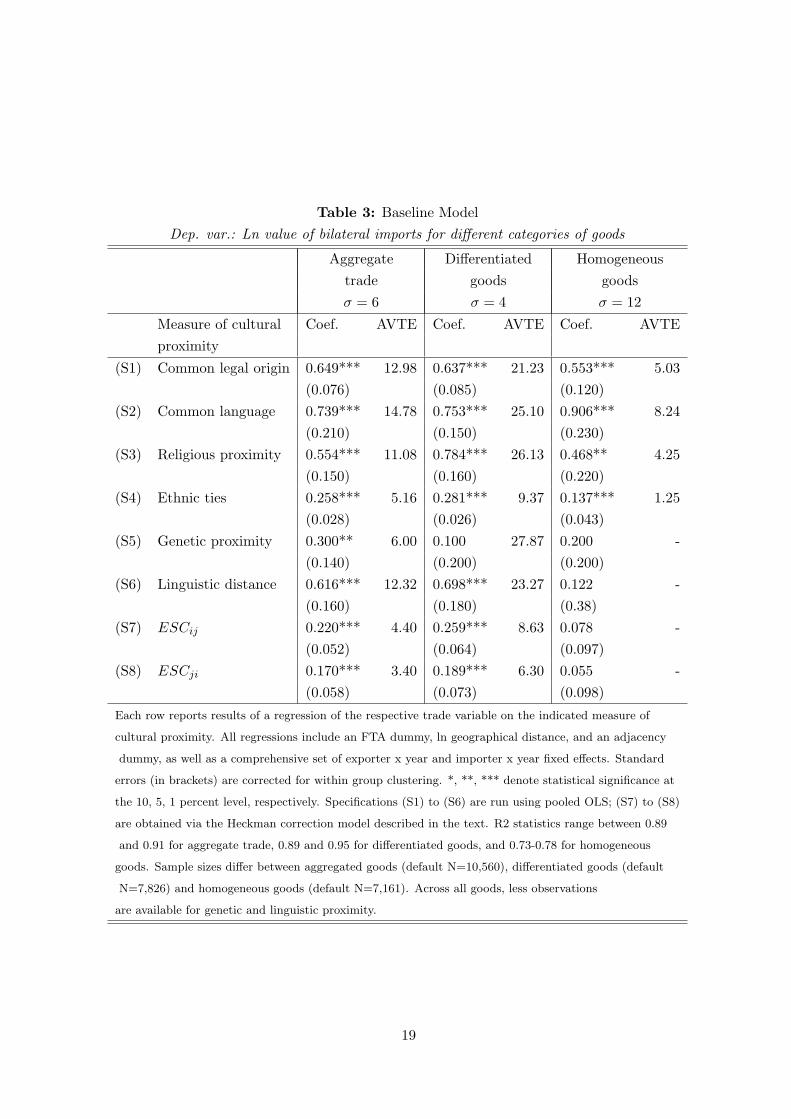
Table 3: Baseline ModelDep. var.: Ln value of bilateral imports for different categories of goods

Aggregate Differentiated Homogeneoustrade goods goodsσ = 6 σ = 4 σ = 12

Measure of cultural Coef. AVTE Coef. AVTE Coef. AVTEproximity

(S1) Common legal origin 0.649*** 12.98 0.637*** 21.23 0.553*** 5.03(0.076) (0.085) (0.120)

(S2) Common language 0.739*** 14.78 0.753*** 25.10 0.906*** 8.24(0.210) (0.150) (0.230)

(S3) Religious proximity 0.554*** 11.08 0.784*** 26.13 0.468** 4.25(0.150) (0.160) (0.220)

(S4) Ethnic ties 0.258*** 5.16 0.281*** 9.37 0.137*** 1.25(0.028) (0.026) (0.043)

(S5) Genetic proximity 0.300** 6.00 0.100 27.87 0.200 -(0.140) (0.200) (0.200)

(S6) Linguistic distance 0.616*** 12.32 0.698*** 23.27 0.122 -(0.160) (0.180) (0.38)

(S7) ESCij 0.220*** 4.40 0.259*** 8.63 0.078 -(0.052) (0.064) (0.097)

(S8) ESCji 0.170*** 3.40 0.189*** 6.30 0.055 -(0.058) (0.073) (0.098)

Each row reports results of a regression of the respective trade variable on the indicated measure of

cultural proximity. All regressions include an FTA dummy, ln geographical distance, and an adjacency

dummy, as well as a comprehensive set of exporter x year and importer x year fixed effects. Standard

errors (in brackets) are corrected for within group clustering. *, **, *** denote statistical significance at

the 10, 5, 1 percent level, respectively. Specifications (S1) to (S6) are run using pooled OLS; (S7) to (S8)

are obtained via the Heckman correction model described in the text. R2 statistics range between 0.89

and 0.91 for aggregate trade, 0.89 and 0.95 for differentiated goods, and 0.73-0.78 for homogeneous

goods. Sample sizes differ between aggregated goods (default N=10,560), differentiated goods (default

N=7,826) and homogeneous goods (default N=7,161). Across all goods, less observations

are available for genetic and linguistic proximity.

19

Let us first focus on aggregate trade. The point estimates of all those measures are precisely

estimated with high levels of significance. The beta coefficient associated to common legal

origin, common language, and religious proximity are 0.0997, 0.0698, and 0.0545 respectively.26

Compared to distance, which has a beta coefficient of about 0.24 (depending on the exact

model), cultural proximity turns out to be an important determinant of bilateral trade volumes.

In specifications (S1) to (S3), the distance elasticity is roughly the same as in specification (S1).

Thus geographical distance is not a substitute measure for the measures of cultural proximity

considered.

Specification (S4) uses ethnic ties as a measure of cultural proximity. The effect of ethnic

ties is somewhat smaller that for the dummy variables discussed above, but is again statistically

significant. Interestingly, including that variable reduces the coefficient of geographical distance

quite substantially. It also comes with a beta coefficient that is an order of magnitude larger

(0.2783). We conclude that in contrast to the measures employed in specifications (S2) to (S4),

ethnic ties convey effects that are similar to distance.

In specification (S5), we find a positive and significant effect of genetic proximity on bilateral

exports. As with ethnic ties, the associated beta coefficient is above 0.2 and the distance coeffi-

cient is substantially lower than unity. However, the underlying sample is smaller. Specification

(S6) uses a continuous variable to measure linguistic proximity between two countries. This

reduces the sample to a third, and dramatically cuts the distance coefficient.

In specifications (S7) to (S8) we use ESC scores as measures of cultural proximity. According

to the Heckman strategy discussed above, we draw only on strictly positive realizations of ESCij

and ESCji. This cuts the number of available observations from 10,560 to 4,833. The Mill’s

ratio is significantly different from zero and strictly positive, which signals that failing to control

for sample selection would overestimate the ESC scores’ coefficients.27 Both Heckman-type

regressions yield coefficients for cultural proximity that are higher for ESCij than for ESCji,

according with intuition. Beta coefficients for ESC scores are 0.029 and 0.023, respectively.

The two regressions differ only with respect to the direction of the scores: in specification (S8),

ESCij measures the score given to j by i, while in specification (S9), ESCji measures the score

given to i by j. One might conjecture that bilateral imports of i from j should depend more

strongly on ESCij than on ESCji, but this expectation does not materialize.

We have computed ad valorem tariff equivalents (AVTE), associated to a change from the

26A beta coefficient is defined as the product of the estimated coefficient and the standard deviation of its

corresponding independent variable, divided by the standard deviation of the dependent variable. It converts the

regression coefficients into units of sample standard deviations.27In line with expectations, without the Heckman correction, estimated coefficients are indeed somewhat larger

(Details are reported in (S8) and (S9) in Table B1 in Appendix B).

20

lowest to the highest sample realization of the respective variable, assuming an elasticity of

substitution of 6. That number ranges from 14.8% for the common language dummy to 11.1%

for religious proximity. Hence, sharing the same language is equivalent to a tariff reduction of

about 18 percentage points. The AVTEs for the Escij scores implied by specifications (S8) and

(S9) are 4.4% and 3.4%, respectively. This is lower than for the conventional measures, pointing

to substantial attenuation bias.

Table 3 also reports the total effect of cultural proximity for differentiated and homogeneous

goods.28 With the exception of genetic proximity, the estimated coefficients are similar to those

found for aggregate trade and estimated with comparable precision. Note, however, that the

time coverage for differentiated and homogeneous goods is 1975 to 2000 instead to 2003 for

aggregate trade. The elasticity of substitution amongst explicitly differentiated goods can be

expected smaller than the average elasticity underlying aggregate trade (Anderson and van

Wincoop, 2004). Assuming σ = 4, we find that the AVTEs are consistently larger (sometimes

twice as large) as those for aggregate trade. In particular, for ESCij we find a tariff equivalent

of 8.63 percent and for ESCji of 6.30 percent. The fact that scores given from i to j matter

substantially more for imports of i from j than the scores given from j to i is in line with the

fact that ESC scores are imperfectly reciprocal.

Turning to the subaggregate of trade in homogeneous goods, we conservatively assume an

elasticity of substitution σ = 12. It turns out that the tariff equivalents associated to the

estimated coefficient for the different measures of cultural proximity are by an order of magnitude

smaller than for trade in differentiated goods, and often statistically identical to zero. This is

a comforting result that accords well with intuition: cultural proximity matters little when

transactions are performed anonymously on organized exchanges.

4.2 Disentangling the trade cost and preference channels

4.2.1 Identification 1: The dyadic fixed effects gravity (DFEG) model

We present the results of our first identification strategy in Tables 4A and 4B. That strategy

draws on Assumption 1, which states that the trade-cost related component of cultural proximity

is time-invariant. In order to quantify the trade costs and preference channel, we proceed in two

steps. First, we estimate equation (11) on aggregate bilateral trade data, including only strictly

positive ESC scores and using a Heckman estimation technique. Second, we include the dyadic

fixed effects in order to tease out the trade costs effect on trade. In Table 4A we use aggregate

bilateral trade as the dependent variable, while in Table 4B we use trade in differentiated and

28Tables B2 and B3 in Appendix B provide full regression output.

21

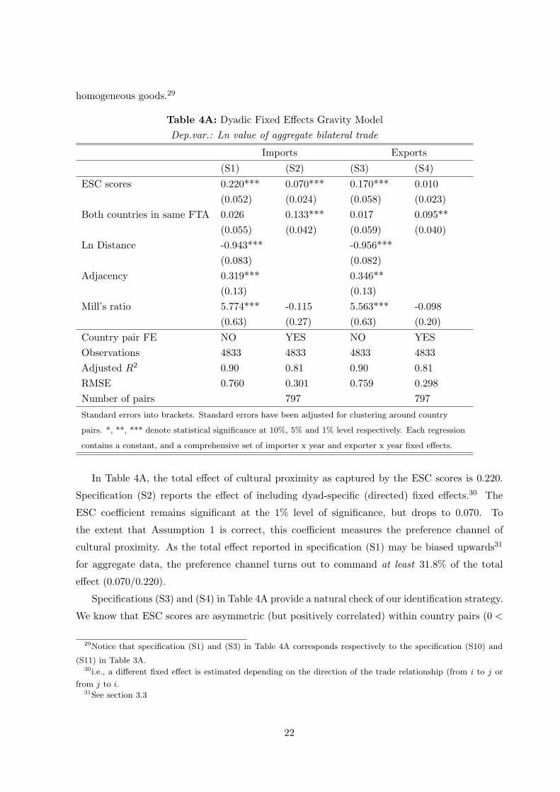
homogeneous goods.29

Table 4A: Dyadic Fixed Effects Gravity ModelDep.var.: Ln value of aggregate bilateral trade

Imports Exports

(S1) (S2) (S3) (S4)

ESC scores 0.220*** 0.070*** 0.170*** 0.010(0.052) (0.024) (0.058) (0.023)

Both countries in same FTA 0.026 0.133*** 0.017 0.095**(0.055) (0.042) (0.059) (0.040)

Ln Distance -0.943*** -0.956***(0.083) (0.082)

Adjacency 0.319*** 0.346**(0.13) (0.13)

Mill’s ratio 5.774*** -0.115 5.563*** -0.098(0.63) (0.27) (0.63) (0.20)

Country pair FE NO YES NO YESObservations 4833 4833 4833 4833Adjusted R2 0.90 0.81 0.90 0.81RMSE 0.760 0.301 0.759 0.298Number of pairs 797 797

Standard errors into brackets. Standard errors have been adjusted for clustering around country

pairs. *, **, *** denote statistical significance at 10%, 5% and 1% level respectively. Each regression

contains a constant, and a comprehensive set of importer x year and exporter x year fixed effects.

In Table 4A, the total effect of cultural proximity as captured by the ESC scores is 0.220.

Specification (S2) reports the effect of including dyad-specific (directed) fixed effects.30 The

ESC coefficient remains significant at the 1% level of significance, but drops to 0.070. To

the extent that Assumption 1 is correct, this coefficient measures the preference channel of

cultural proximity. As the total effect reported in specification (S1) may be biased upwards31

for aggregate data, the preference channel turns out to command at least 31.8% of the total

effect (0.070/0.220).

Specifications (S3) and (S4) in Table 4A provide a natural check of our identification strategy.

We know that ESC scores are asymmetric (but positively correlated) within country pairs (0 <

29Notice that specification (S1) and (S3) in Table 4A corresponds respectively to the specification (S10) and

(S11) in Table 3A.30i.e., a different fixed effect is estimated depending on the direction of the trade relationship (from i to j or

from j to i.31See section 3.3

22

corr(Πijt,Πjit) < 1). Imports of i from j are increased by either Πijt through the trade cost

and/or the preference channels. Exports, however, are increased by Πijt only through the trade

cost channel. They could be affected by the preference channel if Πijt and Πjit were sufficiently

strongly correlated. Hence, if Assumption 1 is true, the effect of ESCijt (as a proxy of Πijt) on

exports should be comparable to its effect on imports. However, the preference channel should

be much smaller for exports than for imports.32 Our results show that this expectation bears

out, supporting the validity of our identification assumption.

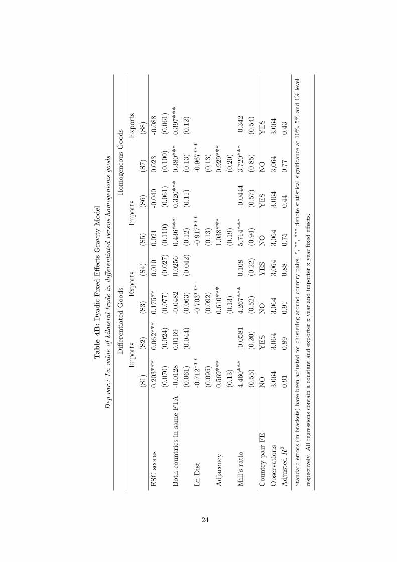
Table 4B repeats the exercise performed in Table 4A using Rauch’s conservative classifica-

tion of goods (Rauch, 1999). We present the results on aggregates of differentiated goods in

specification (S1) to (S4). Specifications (S5) to (S8) present the results for aggregates of homo-

geneous goods. Concerning differentiated goods, the preference effect accounts for at least 30.6%

of the total effect (0.0623/0.203). Again, and comfortingly, the preference channel is absent for

exports.

We do not find any effect of cultural proximity on import and export of homogeneous goods.

However, it is interesting to note that the coefficient of geographical distance seems larger for

homogeneous goods compared to differentiated goods. Hence, the failure of ESCijt to pick up

the trade cost effect might be due to the fact that distance captures the relevant aspects already.

More interestingly, while we do not find any effect of FTA membership for trade in differentiated

goods, we find an effect for trade in homogeneous goods. One reason might lie in the fact that

protectionist policy makers cannot undo the elimination of tariffs on homogeneous goods as

easily as on differentiated goods by introducing non-tariff barriers.

4.2.2 Assumption 2: The bilateral trade balance (BTB) specification

Finally, we turn to the bilateral trade balance equation (13). This equation exploits the as-

sumption 2, which states that trade costs are symmetric between imports and exports. That

assumption is arguably weaker than Assumption 1.

We present the results of the BTB model in Table 5. There are only 903 bilateral relationships

for which both ESCijt and ESCjit are strictly positive. The overall fit of the model is satisfactory

(in particular for differentiated goods), it nevertheless provides a less tested shell for investigation

than the standard gravity equation. For each trade classification, we present two specifications,

one with country pair fixed effects and one without. As argued in section 3.3, we may account

for habit formation by including dyad-specific fixed effects. This turns out to be important

quantitatively.

Specification (S1) and (S2) report the results from using aggregate bilateral trade as de-

32In fact, it should be zero if the theory is correct.

23

Tab

le4B

:D

yadi

cFix

edE

ffect

sG

ravi

tyM

odel

Dep

.var

.:Ln

valu

eof

bila

tera

ltrad

ein

differ

entiat

edve

rsus

hom

ogen

eous

good

s

Diff

eren

tiat

edG

oods

Hom

ogen

eous

Goo

ds

Impo

rts

Exp

orts

Impo

rts

Exp

orts

(S1)

(S2)

(S3)

(S4)

(S5)

(S6)

(S7)

(S8)

ESC

scor

es0.

203*

**0.

062*

**0.

175*

*0.

010

0.02

1-0

.040

0.02

3-0

.088

(0.0

70)

(0.0

24)

(0.0

77)

(0.0

27)

(0.1

10)

(0.0

61)

(0.1

00)

(0.0

61)

Bot

hco

untr

ies

insa

me

FTA

-0.0

128

0.01

69-0

.048

20.

0256

0.43

6***

0.32

0***

0.38

0***

0.39

7***

(0.0

61)

(0.0

44)

(0.0

63)

(0.0

42)

(0.1

2)(0

.11)

(0.1

3)(0

.12)

Ln

Dis

t-0

.712

***

-0.7

03**

*-0

.917

***

-0.9

67**

*(0

.095

)(0

.092

)(0

.13)

(0.1

3)A

djac

ency

0.56

9***

0.61

0***

1.03

8***

0.92

9***

(0.1

3)(0

.13)

(0.1

9)(0

.20)

Mill

’sra

tio

4.46

0***

-0.0

581

4.26

7***

0.10

85.

714*

**-0

.044

43.

720*

**-0

.342

(0.5

5)(0

.20)

(0.5

2)(0

.22)

(0.9

4)(0

.57)

(0.8

5)(0

.54)

Cou

ntry

pair

FE

NO

YE

SN

OY

ES

NO

YE

SN

OY

ES

Obs

erva

tion

s3,

064

3,06

43,

064

3,06

43,

064

3,06

43,

064

3,06

4A

djus

ted

R2

0.91

0.89

0.91

0.88

0.75

0.44

0.77

0.43

Sta

ndard

erro

rs(i

nbra

cket

s)hav

ebee

nadju

sted

for

clust

erin

garo

und

countr

ypair

s.*,**,***

den

ote

stati

stic

alsi

gnifi

cance

at

10%

,5%

and

1%

level

resp

ecti

vel

y.A

llre

gre

ssio

ns

conta

ina

const

ant

and

export

erx

yea

rand

import

erx

yea

rfixed

effec

ts.

24

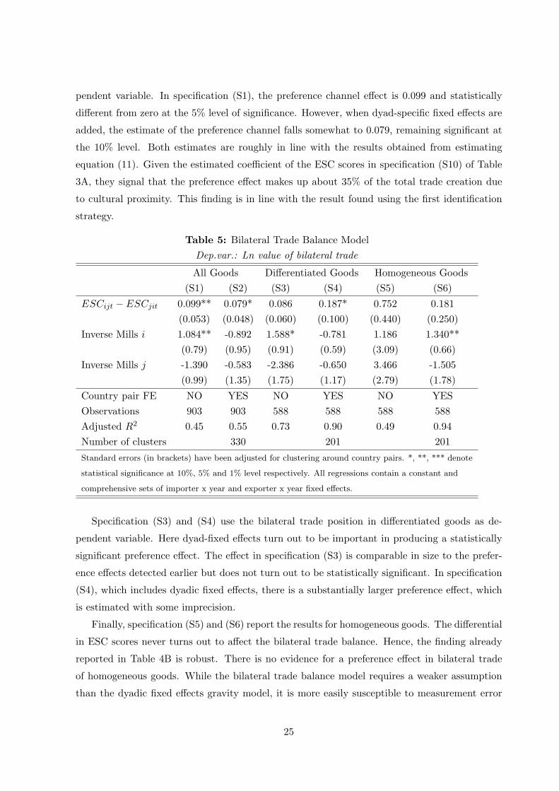
pendent variable. In specification (S1), the preference channel effect is 0.099 and statistically

different from zero at the 5% level of significance. However, when dyad-specific fixed effects are

added, the estimate of the preference channel falls somewhat to 0.079, remaining significant at

the 10% level. Both estimates are roughly in line with the results obtained from estimating

equation (11). Given the estimated coefficient of the ESC scores in specification (S10) of Table

3A, they signal that the preference effect makes up about 35% of the total trade creation due

to cultural proximity. This finding is in line with the result found using the first identification

strategy.

Table 5: Bilateral Trade Balance ModelDep.var.: Ln value of bilateral trade

All Goods Differentiated Goods Homogeneous Goods(S1) (S2) (S3) (S4) (S5) (S6)

ESCijt − ESCjit 0.099** 0.079* 0.086 0.187* 0.752 0.181(0.053) (0.048) (0.060) (0.100) (0.440) (0.250)

Inverse Mills i 1.084** -0.892 1.588* -0.781 1.186 1.340**(0.79) (0.95) (0.91) (0.59) (3.09) (0.66)

Inverse Mills j -1.390 -0.583 -2.386 -0.650 3.466 -1.505(0.99) (1.35) (1.75) (1.17) (2.79) (1.78)

Country pair FE NO YES NO YES NO YESObservations 903 903 588 588 588 588Adjusted R2 0.45 0.55 0.73 0.90 0.49 0.94Number of clusters 330 201 201

Standard errors (in brackets) have been adjusted for clustering around country pairs. *, **, *** denote

statistical significance at 10%, 5% and 1% level respectively. All regressions contain a constant and

comprehensive sets of importer x year and exporter x year fixed effects.

Specification (S3) and (S4) use the bilateral trade position in differentiated goods as de-

pendent variable. Here dyad-fixed effects turn out to be important in producing a statistically

significant preference effect. The effect in specification (S3) is comparable in size to the prefer-

ence effects detected earlier but does not turn out to be statistically significant. In specification

(S4), which includes dyadic fixed effects, there is a substantially larger preference effect, which

is estimated with some imprecision.

Finally, specification (S5) and (S6) report the results for homogeneous goods. The differential

in ESC scores never turns out to affect the bilateral trade balance. Hence, the finding already

reported in Table 4B is robust. There is no evidence for a preference effect in bilateral trade

of homogeneous goods. While the bilateral trade balance model requires a weaker assumption

than the dyadic fixed effects gravity model, it is more easily susceptible to measurement error

25

in the data. However, the results obtained from the trade balance model are largely in line with

those found in Table 4B.

4.3 Robustness checks and instrumental variables results

We have conducted a number of robustness checks, which are reported in detail in an earlier

version of this paper (Felbermayr and Toubal, 2006) or in Appendix B. Here we restrict ourselves

to briefly discuss the most important checks. 33

Table B4 in Appendix B repeats the analysis of Tables 4A and 4B in the text for the

time period 1975-1998, thereby drawing only on scores established by Juries rather than by

televoting. Our main results remain fully intact qualitatively. The total pro-trade effect of

cultural proximity turns out slightly lower, but the preference channel remains of approximately

the same magnitude. Comfortingly, there is no statistically significant preference effect for

exports, neither in the case of aggregate trade nor for differentiated goods. For homogeneous

goods, there is no robust effect of cultural proximity on trade, as in the main body of the paper.

Table B5 provides the results of our IV regressions. We instrument concurrent realizations

of the ESC scores by their fifth lags.34 As Combes et al. (2005) and Guiso et al. (2006) we find

that the IV estimates are much larger than OLS ones. Not surprisingly, they are estimated with

lower precision. However, for the case of trade in differentiated goods, we get relatively accurate

estimates. As the earlier literature, we conclude that reverse causality does not seem to be a

major problem in our regressions since we do not find evidence for an upward bias in the OLS

coefficients.35

Table B6 provides some robustness checks to Table 3 in the text. We use 5th order lags of

ESC scores as dependent variables. Clearly, the number of observations goes down substantially.

As in the IV exercise, our results are most robust in the case of differentiated goods.

Dividing the data into three shorter subsamples 1975-1985, 1986-1995, and 1996-2003, we

find again results in line with those reported in Table 4A. This is important, since Assumption

1 is more likely to hold over shorter time periods. We have also tried to correct for song quality

using a two-stage approach. In the first stage, we use a zero-inflated negative binomial model

to regress scoring outcomes on the outcome of Google counts with the song’s title and the

performing artist/group as search elements, and on a host of observable song characteristics. In

the second stage we use the residuals of this regression as quality adjusted measures of cultural

33Note that in Felbermayr and Toubal (2006), ESC scores are defined with the opposite direction as in the

present paper, and are not normalized to lie in the interval [0, 1].34Shorter lag structures work as well, but to the extent that bilateral trade flows are persistent, are less suited

as instruments. Longer lags yield first stage regressions with fairly low F statistics.35Nevertheless, OLS results may be downward biased due to measurement error. However, the implied mea-

surement error would need to be implausibly large.

26

proximity. It turns out that this procedure delivers results very much in line with those reported

in Table 4A.36

5 Conclusions

Standard measures of cultural proximity, such as common language, common religion, genetic

proximity, etc., do not allow to disentangle the channels through which bilateral trade volumes

are affected: namely, through trade costs and preferences. The first effect obtains when a

higher degree of cultural proximity makes culture-based misunderstandings less likely, leads to

more trust, and therefore lowers transaction costs. The second effect appears when patterns

of cultural proximity across countries are correlated with country-specific weights in the utility

function. Both effects lead to trade creation, but only the former is relevant for welfare. In

the present paper, we have studied the effect on cultural proximity on trade and isolated the

channels through which it matters.

We exploit data from the Eurovision Song Contest (ESC). The ESC is a huge, televised

show, in which European countries grade the songs of other countries. We argue that the

matrix of bilateral votes, obtained in the ESC grading process, can be used as dyadic, time-

variant information on European countries’ cultural proximity. We control for song quality by

including song-specific fixed effects and deal with the peculiarities of the ESC rules (not all

countries are actually ranked). ESC grades correlate strongly with conventional measures of

cultural proximity.

ESC scores have properties that allow to identify the trade-cost and the preference effects

of cultural proximity. Assuming that the trade-cost related component of cultural proximity

is largely time-invariant, the time dimension of the ESC data allows to separately identify

the preferences effect. The validity of our identification strategy can be tested by exploiting

the lack of systematic reciprocity in ESC scores. Our main results are corroborated in a second

identification strategy, where we assume that trade costs are symmetric across a pair of countries,

while preferences need not be.

We find that the total average trade-creating effect of moving cultural proximity from its

lowest to its highest sample values amounts to a tariff equivalent of about 4% for total trade,

and of about 8% for trade in differentiated goods. There is no trade-creating effect of cultural

proximity with homogeneous goods. At least a third of the boost in trade is attributable to the

preference effect.

Our evidence of a statistically and economically sizable preference effect of cultural proximity

establishes an important conceptual difference between geographical proximity, which does not

36Results are available upon request.

27

affect preferences, and cultural proximity. Remote countries, such as New Zealand or Australia,

have more trade than their geographical location would suggest. However, to the extent that

their extra trade is due to preference-driven trade creation, they are still disadvantaged by higher

trade costs.

28

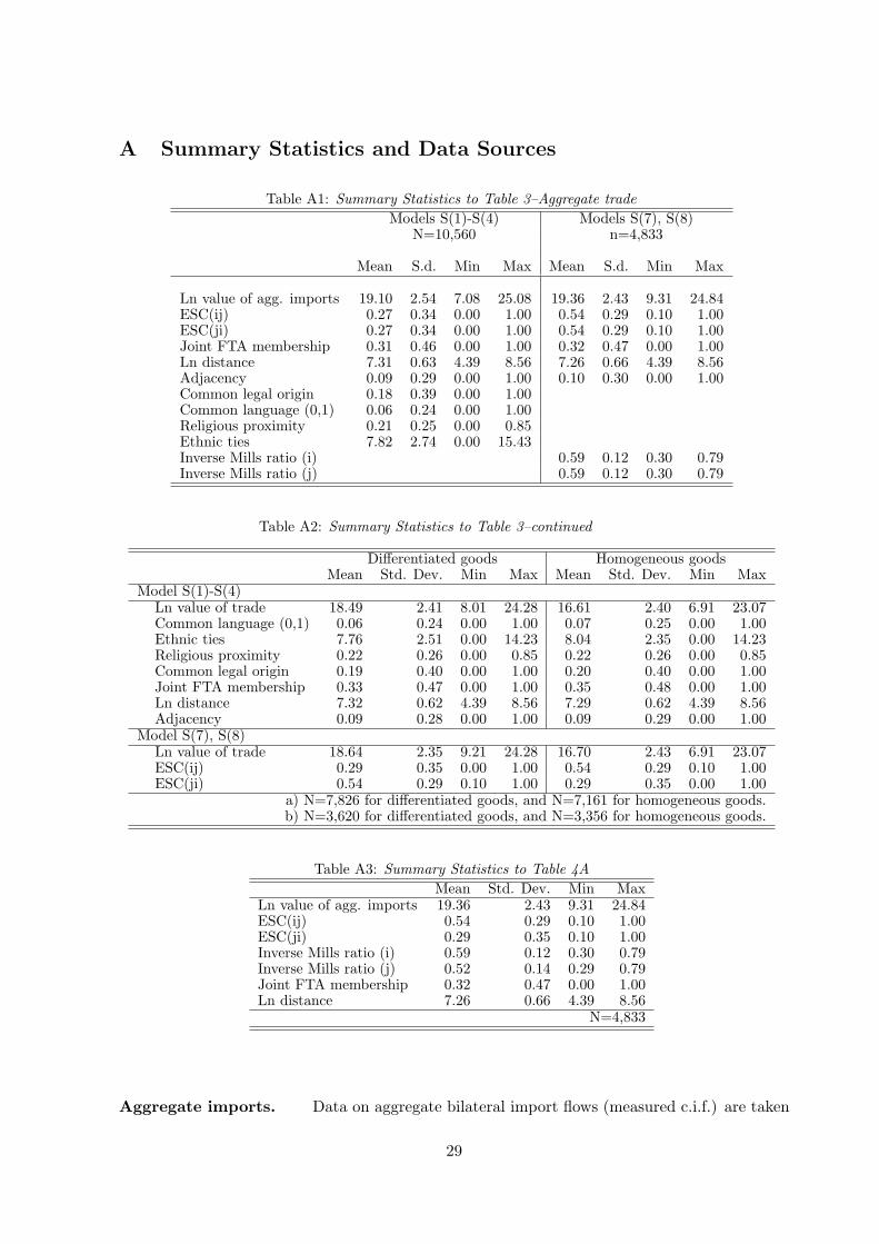
A Summary Statistics and Data Sources

Table A1: Summary Statistics to Table 3–Aggregate tradeModels S(1)-S(4) Models S(7), S(8)

N=10,560 n=4,833

Mean S.d. Min Max Mean S.d. Min Max

Ln value of agg. imports 19.10 2.54 7.08 25.08 19.36 2.43 9.31 24.84ESC(ij) 0.27 0.34 0.00 1.00 0.54 0.29 0.10 1.00ESC(ji) 0.27 0.34 0.00 1.00 0.54 0.29 0.10 1.00Joint FTA membership 0.31 0.46 0.00 1.00 0.32 0.47 0.00 1.00Ln distance 7.31 0.63 4.39 8.56 7.26 0.66 4.39 8.56Adjacency 0.09 0.29 0.00 1.00 0.10 0.30 0.00 1.00Common legal origin 0.18 0.39 0.00 1.00Common language (0,1) 0.06 0.24 0.00 1.00Religious proximity 0.21 0.25 0.00 0.85Ethnic ties 7.82 2.74 0.00 15.43Inverse Mills ratio (i) 0.59 0.12 0.30 0.79Inverse Mills ratio (j) 0.59 0.12 0.30 0.79

Table A2: Summary Statistics to Table 3–continued

Differentiated goods Homogeneous goodsMean Std. Dev. Min Max Mean Std. Dev. Min Max

Model S(1)-S(4)Ln value of trade 18.49 2.41 8.01 24.28 16.61 2.40 6.91 23.07Common language (0,1) 0.06 0.24 0.00 1.00 0.07 0.25 0.00 1.00Ethnic ties 7.76 2.51 0.00 14.23 8.04 2.35 0.00 14.23Religious proximity 0.22 0.26 0.00 0.85 0.22 0.26 0.00 0.85Common legal origin 0.19 0.40 0.00 1.00 0.20 0.40 0.00 1.00Joint FTA membership 0.33 0.47 0.00 1.00 0.35 0.48 0.00 1.00Ln distance 7.32 0.62 4.39 8.56 7.29 0.62 4.39 8.56Adjacency 0.09 0.28 0.00 1.00 0.09 0.29 0.00 1.00

Model S(7), S(8)Ln value of trade 18.64 2.35 9.21 24.28 16.70 2.43 6.91 23.07ESC(ij) 0.29 0.35 0.00 1.00 0.54 0.29 0.10 1.00ESC(ji) 0.54 0.29 0.10 1.00 0.29 0.35 0.00 1.00

a) N=7,826 for differentiated goods, and N=7,161 for homogeneous goods.b) N=3,620 for differentiated goods, and N=3,356 for homogeneous goods.

Table A3: Summary Statistics to Table 4AMean Std. Dev. Min Max

Ln value of agg. imports 19.36 2.43 9.31 24.84ESC(ij) 0.54 0.29 0.10 1.00ESC(ji) 0.29 0.35 0.10 1.00Inverse Mills ratio (i) 0.59 0.12 0.30 0.79Inverse Mills ratio (j) 0.52 0.14 0.29 0.79Joint FTA membership 0.32 0.47 0.00 1.00Ln distance 7.26 0.66 4.39 8.56

N=4,833

Aggregate imports. Data on aggregate bilateral import flows (measured c.i.f.) are taken

29

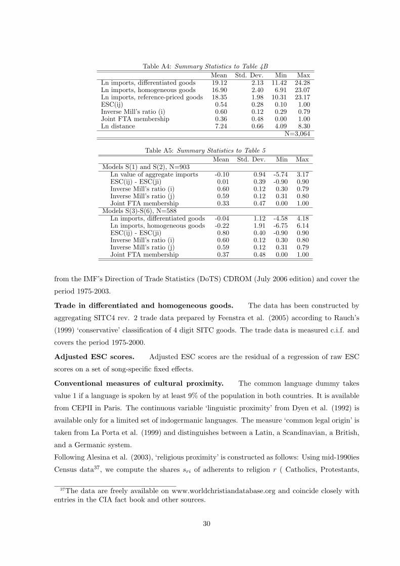
Table A4: Summary Statistics to Table 4BMean Std. Dev. Min Max

Ln imports, differentiated goods 19.12 2.13 11.42 24.28Ln imports, homogeneous goods 16.90 2.40 6.91 23.07Ln imports, reference-priced goods 18.35 1.98 10.31 23.17ESC(ij) 0.54 0.28 0.10 1.00Inverse Mill’s ratio (i) 0.60 0.12 0.29 0.79Joint FTA membership 0.36 0.48 0.00 1.00Ln distance 7.24 0.66 4.09 8.30

N=3,064

Table A5: Summary Statistics to Table 5Mean Std. Dev. Min Max

Models S(1) and S(2), N=903Ln value of aggregate imports -0.10 0.94 -5.74 3.17ESC(ij) - ESC(ji) 0.01 0.39 -0.90 0.90Inverse Mill’s ratio (i) 0.60 0.12 0.30 0.79Inverse Mill’s ratio (j) 0.59 0.12 0.31 0.80Joint FTA membership 0.33 0.47 0.00 1.00

Models S(3)-S(6), N=588Ln imports, differentiated goods -0.04 1.12 -4.58 4.18Ln imports, homogeneous goods -0.22 1.91 -6.75 6.14ESC(ij) - ESC(ji) 0.80 0.40 -0.90 0.90Inverse Mill’s ratio (i) 0.60 0.12 0.30 0.80Inverse Mill’s ratio (j) 0.59 0.12 0.31 0.79Joint FTA membership 0.37 0.48 0.00 1.00

from the IMF’s Direction of Trade Statistics (DoTS) CDROM (July 2006 edition) and cover the

period 1975-2003.

Trade in differentiated and homogeneous goods. The data has been constructed by

aggregating SITC4 rev. 2 trade data prepared by Feenstra et al. (2005) according to Rauch’s

(1999) ‘conservative’ classification of 4 digit SITC goods. The trade data is measured c.i.f. and

covers the period 1975-2000.

Adjusted ESC scores. Adjusted ESC scores are the residual of a regression of raw ESC

scores on a set of song-specific fixed effects.

Conventional measures of cultural proximity. The common language dummy takes

value 1 if a language is spoken by at least 9% of the population in both countries. It is available

from CEPII in Paris. The continuous variable ‘linguistic proximity’ from Dyen et al. (1992) is

available only for a limited set of indogermanic languages. The measure ‘common legal origin’ is

taken from La Porta et al. (1999) and distinguishes between a Latin, a Scandinavian, a British,

and a Germanic system.

Following Alesina et al. (2003), ‘religious proximity’ is constructed as follows: Using mid-1990ies

Census data37, we compute the shares sri of adherents to religion r ( Catholics, Protestants,

37The data are freely available on www.worldchristiandatabase.org and coincide closely withentries in the CIA fact book and other sources.

30

orthodox Christians, Muslims, Jews, atheists, and non-religious persons) in total population of

country i. Then, we compute a bilateral index ρij =∑

r srisrj , with ρij ∈ [0, 1] . This measure

reaches a maximum value of 0.85 for the dyad Poland-Malta, and is minimum, 0.001, for the

pair Poland-Turkey.

As a measure of ethnic ties, we use the stock of foreign born individuals by country of birth,

provided by the OECD and discussed in Dumont and Lemaitre (2005). Finally, we use data on

genetic distance computed by Cavalli-Sforza (1994) and made available by Paola Giuliano.

Geographical data. Data on geographical distance and on adjacency is taken from the

CEPII in Paris.38

Free trade agreements. Data is from Baier and Bergstrand (2006) and updated for ac-

count for the pre-EU membership Europe agreements signed by East European countries with

the EU (WTO website).

38The CEPII data can be downloaded from www.cepii.fr/anglaisgraph/ bdd/distances.htm.

31

References

[1] Alesina, A., Dollar, D., 2002. Who Gives Foreign Aid to Whom and Why. Journal of

Economic Growth 5, 33-64.

[2] Anderson, J.E., Van Wincoop, E., 2003, Gravity with Gravitas: A Solution to the Border

Puzzle. American Economic Review 03(1): 170-192.

[3] Anderson, J.E., Van Wincoop, E., 2004, Trade Costs. Journal of Economic Literature 32(3):

691-751.

[4] Baier, S.L., Bergstrand, J.H., 2006, Do Free Trade Agreements Actually Increase Members’

International Trade? Journal of International Economics, forthcoming.

[5] Baltagi, B.H., Egger, P., Pfaffermayr, M., 2003, A Generalized Design For Bilateral Trade

Flow Models. Economics Letters 80: 391-397.

[6] Borjas, G., 1987. Self-Selection and the Earnings of Immigrants. American Economic Re-

view: 531-553.

[7] Boisso, D., Ferrantino, M., 1997, Economic Distance, Cultural Distance, and Openness in

International Trade: Empirical Puzzles. Journal of Economic Integration 12(4): 456-484.

[8] Casella, A., Rauch, J., 2003. Overcoming Informational Barrier to International Resource

Allocation. Prices and Ties. Economic Journal 113(1): 21-42.

[9] Cavalli-Sforza, L., P.Menozzi, and A. Piazza, 1994, The History and Geography of Human

Genes. Princeton, New Jersey: Princeton University Press.

[10] Clerides, S., Stengos, T., 2006. Love thy Neighbor, Love thy Kin: Voting Biases in the

Eurovision Song Contest. Mimeo: University of Cyprus.

[11] Combes, P-P., M. Lafourcade and T. Mayer, 2005. The Trade Creating Effects of Business

and Social Networks: Evidence from France, Journal of International Economics 66:1-29.

[12] Davis, D.R., Weinstein, D.E., 2002. The Mystery of Excess Trade (Balances). American

Economic Review 92(2): 170-174.

[13] Davis, D., Weinstein, D., 2003. Market Access, Economic Geography and Comparative

Advantage: An Empirical Assessment,” Journal of International Economics 59(1): 1-23.

[14] Disdier, A.C., Mayer, T., 2006. Je T’aime, Moi Non Plus. Bilateral Opinions and Interna-

tional Trade. European Journal of Political Economy, forthocming.

32

[15] Dumont, J.-C. and Lemaitre, G., 2005, Counting immigrants and expatri- ates: A new

perspective. OECD Social, Employment and MigrationWorking Paper 25.

[16] Dyen, I., Kruskal, J.B., and Black, P., 1992. An Indoeuropean Classification: A Lexicosta-

tistical Experiment. Transactions of the American Philosophical Society 82(5).

[17] Feenstra, R. C., 2004. Advanced International Trade. Theory and Evidence. Princeton:

Princeton University Press.

[18] Feenstra, R. C., Lipsey, R.E., Deng, H., Ma, A.C., and Mo, H., 2005. World Trade Flows:

1962-2000. NBER Working Paper 11040.

[19] Fenn, D., O. Suleman, Efstathiou, J., Johnson, N.F., 2006. How does Europe Make Its

Mind Up? Connections, cliques, and compatibility between countries in the Eurovision

Song Contest. Physica A 360(2): 576-598.

[20] Fernandez, R., 2007. Culture and Economics. New Palgrave Dictionary of Economics, 2nd

ed., edited by Durlauf, S.N., and Blume, L.E., Palgrave McMillan, New York.

[21] Frankel, J.A., Romer, D., 1999. Does trade cause growth? American Economic Review

89(3): 379–399.

[22] Ginsburgh, V., Noury, A., 2004. Cultural Voting: The Eurovision Song Contest. Universite

Libre de Bruxelles, mimeo.

[23] Ginsburgh, V., 2005. Languages, Genes, and Cultures. Journal of Cultural Econonomics

29(1), 1-17.

[24] Giuliano, P., Spilimbergo, A., and Tonon, G., 2006. Genetic, Cultural and Geographical

Distances. IZA Working Paper 2229.

[25] Guiso, L., Sapienza, P., and Zingales, L., 2004. Cultural Biases in Economic Exchange.

NBER Working Paper 11005.

[26] Guiso, L., Sapienza, P., and Zingales, L., 2006. Does Culture Affect Economic Outcomes?

Journal of Economic Perspectives 20(2): 23-48.

[27] Haan, M.A., Djikstra, G.S., Dijkstra, P.T., 2005. Expert Judgment versus Public Opinion.

Evidence from the Eurovision Song Contest. Journal of Cultural Economics 29(1): 59-78.

[28] Hanson, G.H., and Xiang, C., 2004. The Home Market Effect and Bilateral Trade Patterns.

American Economic Review 94(4): 1108-1129.

33

[29] Heckman, James J., 1979. Sample Selection Bias as a Specification Error. Econometrica

47(1):153-161.

[30] Helpman, E., 1987. Imperfect Competition and International Trade. Evidence from Four-

teen Industrialized Countries. Journal of the Japanese and International Economies 1: 62-

81.

[31] Huang, R.R., 2007. Distance and Trade: Disentangling Unfamiliarity Effects and Trans-

portation Cost Effects. European Economic Review 51: 161-181.

[32] Hutchinson, W., 2006. Linguistic Distance as a Determinant of U.S. Bilateral Trade, 1970-

1986. Southern Economic Journal 72(1): 1-15.

[33] La Porta, R., Shleifer, A., Vishny, R.W., Lopez Da Silanes, F., 1998. Law and Finance.

Journal of Political Economy 106(6).

[34] Melitz, J., 2002, Language and Foreign Trade, CEPR Discussion Paper 3590.

[35] Manski, C.F., 2000. Economic Analysis of Social Interactions. Journal of Economic Per-

spectives 14(3): 115-136.

[36] Rauch, J.E., 1999. Networks Versus Markets in International Trade. Journal of International

Economics 48(1): 7-35.

[37] Rauch, J.E., Trindade, V., 2002. Ethnic Chinese Networks in International Trade. Review

of Economics and Statistics 84(1): 116-130

[38] Redding, S., Venables, A.J., 2004. Economic Geography and International Inequality. Jour-

nal of International Economics 62(1): 53-82.

[39] Rose, A.K., 2004. Do We Really Know that the WTO raises trade? American Economic

Review 94(1): 98-114.

[40] Spierdijek, L. and Vellekoop, M., 2006. Geography, Culture, and Religion: Explaining the

Bias in Eurovision Song Contest Voting. Mimeo: University of Twente.

[41] Spolaore, E., and Wacziarg, R., 2006. The Diffusion of Development. NBER Working Paper

12153.

[42] Straubhaar, J., 2002. (Re)asserting national television and national identity against the

global, regional and local levels of world television. In J. M. Chan and B. T. McIntyre (eds.):

In search of boundaries. Communication, nation-States and cultural identities. Westport,

Connecticut: Ablex Publishing.

34

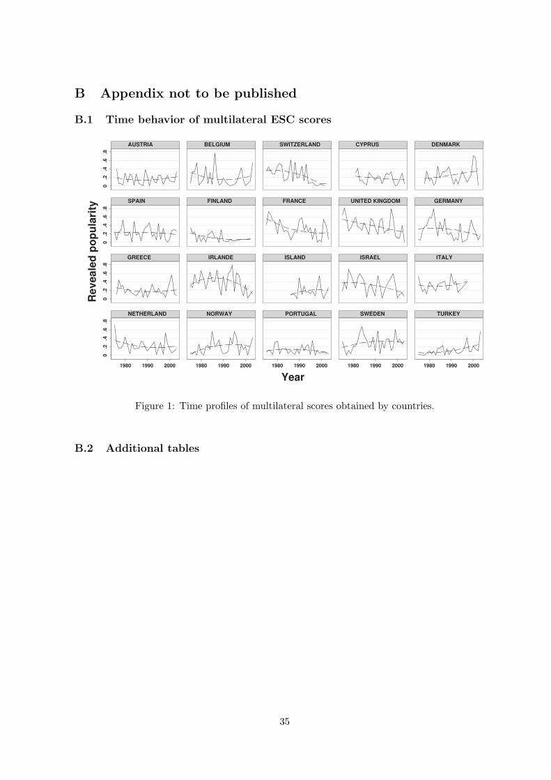
B Appendix not to be published

B.1 Time behavior of multilateral ESC scores

0.2

.4.6

.80

.2.4

.6.8

0.2

.4.6

.80

.2.4

.6.8

1980 1990 2000 1980 1990 2000 1980 1990 2000 1980 1990 2000 1980 1990 2000

AUSTRIA BELGIUM SWITZERLAND CYPRUS DENMARK

SPAIN FINLAND FRANCE UNITED KINGDOM GERMANY

GREECE IRLANDE ISLAND ISRAEL ITALY

NETHERLAND NORWAY PORTUGAL SWEDEN TURKEY

Re

ve

ale

d p

op

ula

rity

Year

Figure 1: Time profiles of multilateral scores obtained by countries.

B.2 Additional tables

35

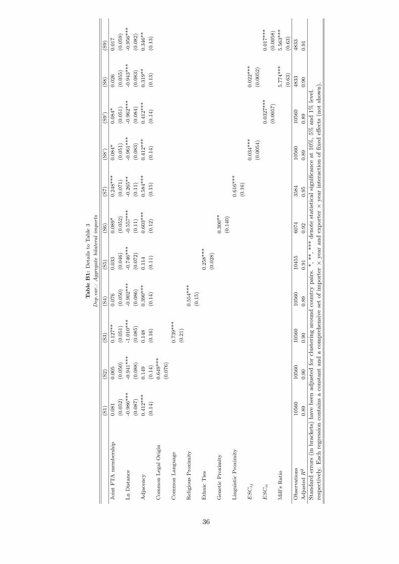
Table

B1:

Det

ails

toTable

3

Dep

.var.

:Agg

rega

tebi

late

ralim

port

s

(S1)

(S2)

(S3)

(S4)

(S5)

(S6)

(S7)

(S8’)

(S9’)

(S8)

(S9)

Join

tFTA

mem

ber

ship

0.0

81

0.0

05

0.1

27**

0.0

76

0.0

33

0.0

89*

0.2

48***

0.0

84*

0.0

84*

0.0

26

0.0

17

(0.0

52)

(0.0

50)

(0.0

51)

(0.0

50)

(0.0

46)

(0.0

52)

(0.0

71)

(0.0

51)

(0.0

51)

(0.0

55)

(0.0

59)

Ln

Dis

tance

-0.9

86***

-0.9

41***

-1.0

10***

-0.9

02***

-0.7

46***

-0.5

57***

-0.2

65**

-0.9

61***

-0.9

62***

-0.9

43***

-0.9

56***

(0.0

87)

(0.0

88)

(0.0

85)

(0.0

86)

(0.0

72)

(0.1

1)

(0.1

1)

(0.0

83)

(0.0

84)

(0.0

83)

(0.0

82)

Adja

cency

0.4

12***

0.1

49

0.1

48

0.3

90***

0.1

14

0.6

03***

0.5

84***

0.4

12***

0.4

12***

0.3

19**

0.3

46**

(0.1

4)

(0.1

4)

(0.1

6)

(0.1

4)

(0.1

1)

(0.1

2)

(0.1

5)

(0.1

4)

(0.1

4)

(0.1

3)

(0.1

3)

Com

mon

Leg

alO

rigin

0.6

49***

(0.0

76)

Com

mon

Language

0.7

39***

(0.2

1)

Rel

igio

us

Pro

xim

ity

0.5

54***

(0.1

5)

Eth

nic

Tie

s0.2

58***

(0.0

28)

Gen

etic

Pro

xim

ity

0.3

00**

(0.1

40)

Lin

guis

tic

Pro

xim

ity

0.6

16***

(0.1

6)

ES

Cij

0.0

34***

0.0

22***

(0.0

054)

(0.0

052)

ES

Cii

0.0

327***

0.0

17***

(0.0

057)

(0.0

058)

Mill’s

Rati

o5.7

74***

5.5

63***

(0.6

3)

(0.6

3)

Obse

rvati

ons

10560

10560

10560

10560

10455

6074

3584

10560

10560

4833

4833

Adju

sted

R2

0.8

90.9

00.9

00.8

90.9

10.9

20.9

50.8

90.8

90.9

00.9

1

Sta

ndard

erro

rs(i

nbra

cket

s)hav

ebee

nadju

sted

for

clust

erin

garo

und

countr

ypair

s.*,**,***

den

ote

stati

stic

alsi

gnifi

cance

at

10%

,5%

and

1%

level

.

resp

ecti

vel

y.E

ach

regre

ssio

nco

nta

ins

aco

nst

ant

and

aco

mpre

hen

sive

set

ofim

port

er×

yea

rand

export

er×

yea

rin

tera

ctio

noffixed

effec

ts(n

ot

show

n).

36

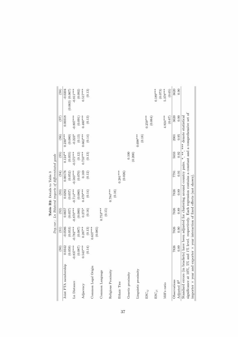
Table

B2:

Det

ails

toTable

3

Dep

.var.

:Ln

Bilate

ralim

port

sofdiff

eren

tiate

dgo

ods

(S0)

(S1)

(S2)

(S3)

(S4)

(S5)

(S6)

(S7)

(S8)

Join

tFTA

mem

ber

ship

0.0

342

-0.0

586

0.0

657

0.0

292

0.0

0176

0.1

24**

0.2

30***

0.0

0318

-0.0

204

(0.0

59)

(0.0

53)

(0.0

57)

(0.0

57)

(0.0

52)

(0.0

55)

(0.0

80)

(0.0

63)

(0.0

67)

Ln

Dis

tance

-0.8

37***

-0.7

82***

-0.8

70***

-0.7

14***

-0.5

83***

-0.5

75***

-0.2

23*

-0.8

07***

-0.8

11***

(0.0

87)

(0.0

87)

(0.0

80)

(0.0

80)

(0.0

70)

(0.1

2)

(0.1

3)

(0.0

91)

(0.0

92)

Adja

cency

0.5

43***

0.2

87**

0.2

75*

0.4

79***

0.1

69

0.7

33***

0.6

62***

0.4

80***

0.5

17***

(0.1

4)

(0.1

3)

(0.1

6)

(0.1

4)

(0.1

2)

(0.1

3)

(0.1

4)

(0.1

3)

(0.1

3)

Com

mon

Leg

alO

rigin

0.6

37***

(0.0

85)

Com

mon

Language

0.7

53***

(0.1

5)

Rel

igio

us

Pro

xim

ity

0.7

84***

(0.1

6)

Eth

nic

Tie

s0.2

81***

(0.0

26)

Gen

etic

pro

xim

ity

0.1

00

(0.2

00)

Lin

guis

tic

pro

xim

ity

0.6

98***

(0.1

8)

ESC

ij0.2

59***

(0.0

64)

ESC

ji

0.1

89***

(0.0

73)

Mill’s

rati

o4.9

24***

5.3

78***

(0.6

7)

(0.6

5)

Obse

rvati

ons

7826

7826

7826

7826

7791

5033

2901

3620

3620

Adju

sted

R2

0.8

90.9

00.8

90.8

90.9

10.9

20.9

50.9

00.9

0

Sta

ndard

erro

rs(i

nbra

cket

s)hav

ebee

nadju

sted

for

clust

erin

garo

und

countr

ypair

s.*,**,***

den

ote

stati

stic

al

signifi

cance

at

10%

,5%

and

1%

level

.re

spec

tivel

y.E

ach

regre

ssio

nco

nta

ins

aco

nst

ant

and

aco

mpre

hen

sive

set

of

import

er×

yea

rand

export

er×

yea

rin

tera

ctio

noffixed

effec

ts(n

ot

show

n).

37

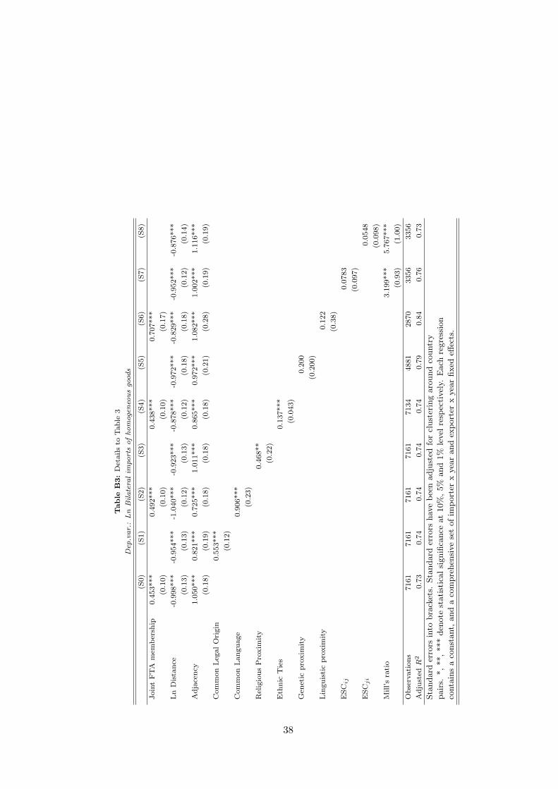
Table

B3:

Det

ails

toTable

3

Dep

.var.

:Ln

Bilate

ralim

port

sofhom

ogen

eous

good

s

(S0)

(S1)

(S2)

(S3)

(S4)

(S5)

(S6)

(S7)

(S8)

Join

tFTA

mem

ber

ship

0.4

53***

0.4

92***

0.4

38***

0.7

07***

(0.1

0)

(0.1

0)

(0.1

0)

(0.1

7)

Ln

Dis

tance

-0.9

98***

-0.9

54***

-1.0

40***

-0.9

23***

-0.8

78***

-0.9

72***

-0.8

29***

-0.9

52***

-0.8

76***

(0.1

3)

(0.1

3)

(0.1

2)

(0.1

3)

(0.1

2)

(0.1

8)

(0.1

8)

(0.1

2)

(0.1

4)

Adja

cency

1.0

50***

0.8

21***

0.7

25***

1.0

11***

0.8

65***

0.9

72***

1.0

82***

1.0

02***

1.1

16***

(0.1

8)

(0.1

9)

(0.1

8)

(0.1

8)

(0.1

8)

(0.2

1)

(0.2

8)

(0.1

9)

(0.1

9)

Com

mon

Leg

alO

rigin

0.5

53***

(0.1

2)

Com

mon

Language

0.9

06***

(0.2

3)

Rel

igio

us

Pro

xim

ity

0.4

68**

(0.2

2)

Eth

nic

Tie

s0.1

37***

(0.0

43)

Gen

etic

pro

xim

ity

0.2

00

(0.2

00)

Lin

guis

tic

pro

xim

ity

0.1

22

(0.3

8)

ESC

ij0.0

783

(0.0

97)

ESC

ji

0.0

548

(0.0

98)

Mill’s

rati

o3.1

99***

5.7

67***

(0.9

3)

(1.0

0)

Obse

rvati

ons

7161

7161

7161

7161

7134

4881

2870

3356

3356

Adju

sted

R2

0.7

30.7

40.7

40.7

40.7

40.7

90.8

40.7

60.7

3

Sta

ndard

erro

rsin

tobra

cket

s.Sta

ndard

erro

rshav

ebee

nadju

sted

for

clust

erin

garo

und

countr

y

pair

s.*,**,***

den

ote

stati

stic

alsi

gnifi

cance

at

10%

,5%

and

1%

level

resp

ecti

vel

y.E

ach

regre

ssio

n

conta

ins

aco

nst

ant,

and

aco

mpre

hen

sive

set

ofim

port

erx

yea

rand

export

erx

yea

rfixed

effec

ts.

38

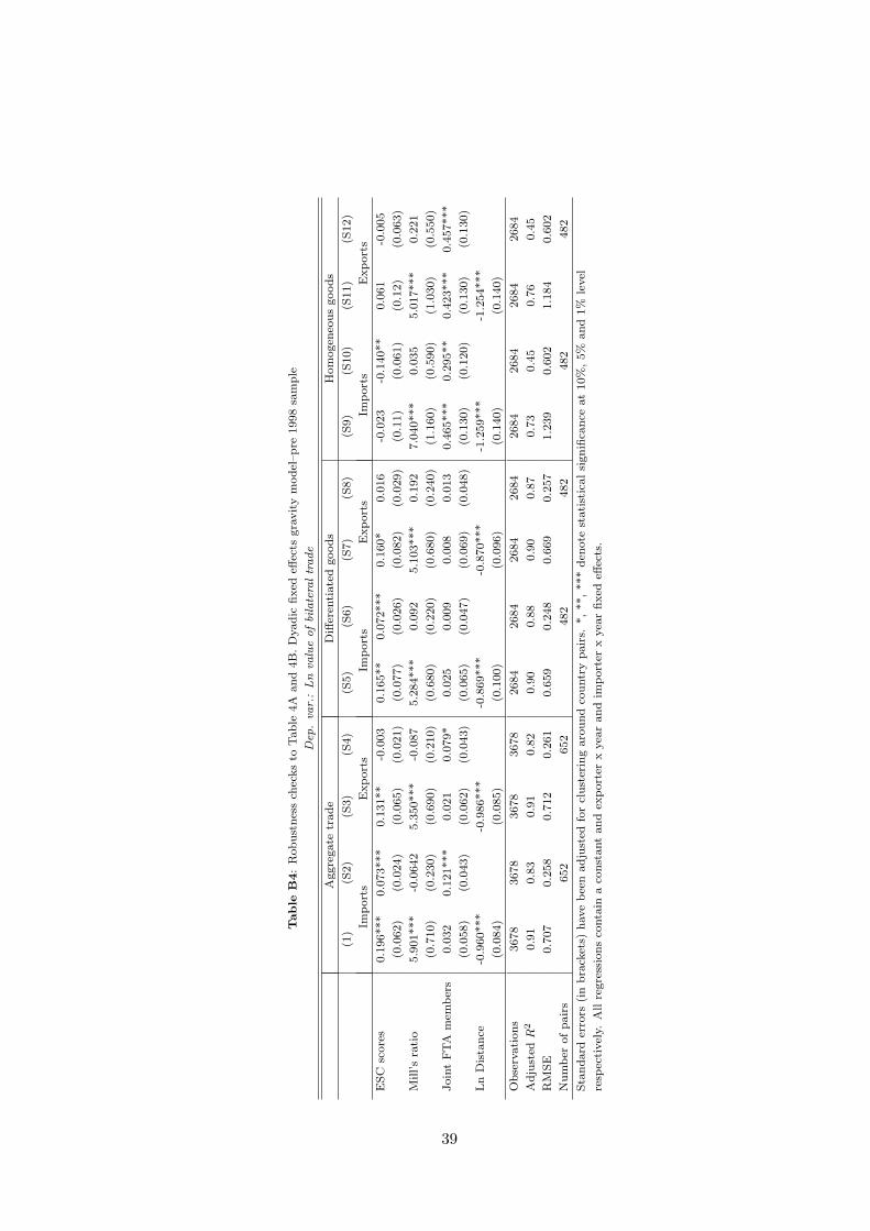
Table

B4:

Robust

nes

sch

ecks

toTable

4A

and

4B

.D

yadic

fixed

effec

tsgra

vity

model

–pre

1998

sam

ple

Dep

.va

r.:

Ln

valu

eofbi

late

raltrade

Aggre

gate

trade

Diff

eren

tiate

dgoods

Hom

ogen

eous

goods

(1)

(S2)

(S3)

(S4)

(S5)

(S6)

(S7)

(S8)

(S9)

(S10)

(S11)

(S12)

Import

sE

xport

sIm

port

sE

xport

sIm

port

sE

xport

s

ESC

score

s0.1

96***

0.0

73***

0.1

31**

-0.0

03

0.1

65**

0.0

72***

0.1

60*

0.0

16

-0.0

23

-0.1

40**

0.0

61

-0.0

05

(0.0

62)

(0.0

24)

(0.0

65)

(0.0

21)

(0.0

77)

(0.0

26)

(0.0

82)

(0.0

29)

(0.1

1)

(0.0

61)

(0.1

2)

(0.0

63)

Mill’s

rati

o5.9

01***

-0.0

642

5.3

50***

-0.0

87

5.2

84***

0.0

92

5.1

03***

0.1

92

7.0

40***

0.0

35

5.0

17***

0.2

21

(0.7

10)

(0.2

30)

(0.6

90)

(0.2

10)

(0.6

80)

(0.2

20)

(0.6

80)

(0.2

40)

(1.1

60)

(0.5

90)

(1.0

30)

(0.5

50)

Join

tFTA

mem

ber

s0.0

32

0.1

21***

0.0

21

0.0

79*

0.0

25

0.0

09

0.0

08

0.0

13

0.4

65***

0.2

95**

0.4

23***

0.4

57***

(0.0

58)

(0.0

43)

(0.0

62)

(0.0

43)

(0.0

65)

(0.0

47)

(0.0

69)

(0.0

48)

(0.1

30)

(0.1

20)

(0.1

30)

(0.1

30)

Ln

Dis

tance

-0.9

60***

-0.9

86***

-0.8

69***

-0.8

70***

-1.2

59***

-1.2

54***

(0.0

84)

(0.0

85)

(0.1

00)

(0.0

96)

(0.1

40)

(0.1

40)

Obse

rvati

ons

3678

3678

3678

3678

2684

2684

2684

2684

2684

2684

2684

2684

Adju

sted

R2

0.9

10.8

30.9

10.8

20.9

00.8

80.9

00.8

70.7

30.4

50.7

60.4

5

RM

SE

0.7

07

0.2

58

0.7

12

0.2

61

0.6

59

0.2

48

0.6

69

0.2

57

1.2

39

0.6

02

1.1

84

0.6

02

Num

ber

ofpair

s652

652

482

482

482

482

Sta

ndard

erro

rs(i

nbra

cket

s)have

bee

nadju

sted

for

clust

erin

garo

und

countr

ypair

s.*,**,***

den

ote

stati

stic

alsi

gnifi

cance

at

10%

,5%

and

1%

level

resp

ecti

vel

y.A

llre

gre

ssio

ns

conta

ina

const

ant

and

export

erx

yea

rand

import

erx

yea

rfixed

effec

ts.

39

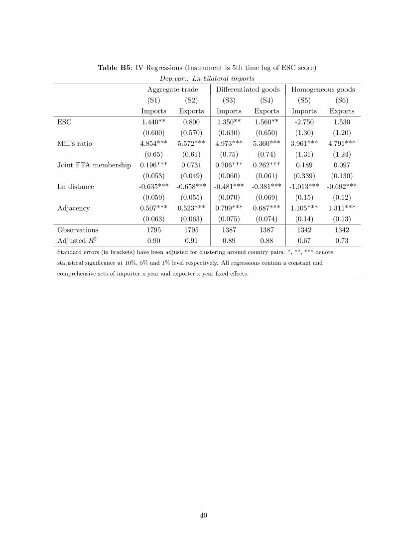
Table B5: IV Regressions (Instrument is 5th time lag of ESC score)Dep.var.: Ln bilateral imports

Aggregate trade Differentiated goods Homogeneous goods(S1) (S2) (S3) (S4) (S5) (S6)

Imports Exports Imports Exports Imports Exports

ESC 1.440** 0.800 1.350** 1.560** -2.750 1.530(0.600) (0.570) (0.630) (0.650) (1.30) (1.20)

Mill’s ratio 4.854*** 5.572*** 4.973*** 5.360*** 3.961*** 4.791***(0.65) (0.61) (0.75) (0.74) (1.31) (1.24)

Joint FTA membership 0.196*** 0.0731 0.206*** 0.262*** 0.189 0.097(0.053) (0.049) (0.060) (0.061) (0.339) (0.130)

Ln distance -0.635*** -0.658*** -0.481*** -0.381*** -1.013*** -0.692***(0.059) (0.055) (0.070) (0.069) (0.15) (0.12)

Adjacency 0.507*** 0.523*** 0.799*** 0.687*** 1.105*** 1.311***(0.063) (0.063) (0.075) (0.074) (0.14) (0.13)

Observations 1795 1795 1387 1387 1342 1342Adjusted R2 0.90 0.91 0.89 0.88 0.67 0.73

Standard errors (in brackets) have been adjusted for clustering around country pairs. *, **, *** denote

statistical significance at 10%, 5% and 1% level respectively. All regressions contain a constant and

comprehensive sets of importer x year and exporter x year fixed effects.

40

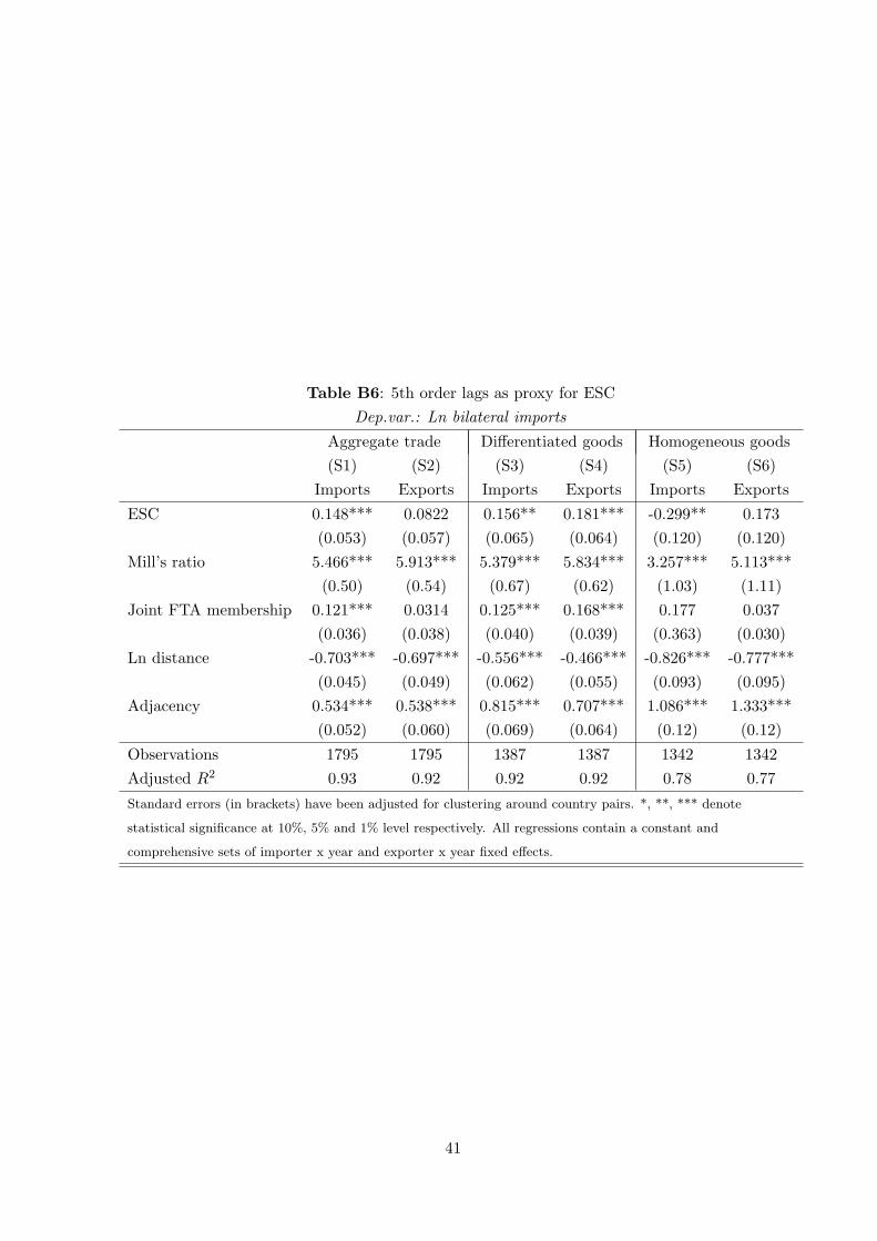
Table B6: 5th order lags as proxy for ESCDep.var.: Ln bilateral imports

Aggregate trade Differentiated goods Homogeneous goods(S1) (S2) (S3) (S4) (S5) (S6)

Imports Exports Imports Exports Imports Exports

ESC 0.148*** 0.0822 0.156** 0.181*** -0.299** 0.173(0.053) (0.057) (0.065) (0.064) (0.120) (0.120)

Mill’s ratio 5.466*** 5.913*** 5.379*** 5.834*** 3.257*** 5.113***(0.50) (0.54) (0.67) (0.62) (1.03) (1.11)

Joint FTA membership 0.121*** 0.0314 0.125*** 0.168*** 0.177 0.037(0.036) (0.038) (0.040) (0.039) (0.363) (0.030)

Ln distance -0.703*** -0.697*** -0.556*** -0.466*** -0.826*** -0.777***(0.045) (0.049) (0.062) (0.055) (0.093) (0.095)

Adjacency 0.534*** 0.538*** 0.815*** 0.707*** 1.086*** 1.333***(0.052) (0.060) (0.069) (0.064) (0.12) (0.12)

Observations 1795 1795 1387 1387 1342 1342Adjusted R2 0.93 0.92 0.92 0.92 0.78 0.77

Standard errors (in brackets) have been adjusted for clustering around country pairs. *, **, *** denote

statistical significance at 10%, 5% and 1% level respectively. All regressions contain a constant and

comprehensive sets of importer x year and exporter x year fixed effects.

41