Cubature Filters - EURASIP · Webiner, CISDA Tutorial, Ottawa, July 2009 (Haykin) 1 Cubature Filters: New Generation of Nonlinear Filters that will Impact the Literature

1

t will

Webiner, CISDA Tutorial, Ottawa, July 2009 (Haykin)

Cubature Filters:New Generation of Nonlinear Filters tha

Impact the Literature

Simon HaykinMcMaster, University

Hamilton, Ontario, Canada

email: [email protected] site: http://soma.mcmaster.ca

2

an Filter

terlinear Systems

ork


Outline of The Lecture

1. Introductory Remarks2. The Bayesian Filter3. Two Approaches for Approximating the Bayesi4. The Cubature Kalman Filter5. Unique Properties of the Cubature Kalman Fil6. Cubature Filtering for Continuous-Discrete non7. Applications of Cubature Filters8. Example I: Tracking a Manoeuvring ship9. Example II: Training a Recurrent Neural Netw10. Concluding Remarks

3

ity may not be

f the problem

a sub-optimal


1. Introductory Remarks

“Optimality versus Robustness”

In many algorithmic applications, global optimalpractically feasible:

(i) Naturally infeasible computability(ii) Curse-of-dimensionality due to large-scale nature o

at hand

Hence, the practical requirement of having to settle for solution of the system design, which involves:

Trade-off between two conflicting design objectives:• global optimality• computational tractability and robust behaviour

4

E

brain does on a

bleesources.

-dependent.


Criterion for sub-optimality

DO AS BEST AS YOU CAN, AND NOT MOR

• This statement is the essence of what the humandaily basis:

Provide the “best” solution in the most reliafashion for the task at hand, given limited r

• Key question: How do we define “best”?

Naturally, the answer to this question is problem

5

ee, 1964)

idden state of theence of noisy

for the optimal.

esian filter is note form of


2. The Bayesian Filter (Ho and L

Problem statement:

Given a nonlinear dynamic system, estimate the hsystem in a recursive manner by processing a sequobservations dependent on the state.

• The Bayesian filter provides a unifying framework solution of this problem, at least in conceptual sense

Unfortunately, except in a few special cases, the Bayimplementable in practice -- hence, the need for somapproximation.

6

:

ear equation:(1)

nlinear

(2)


State-space Model of a Nonlinear Dynamic System

1. Process (state) sub-model defined by the nonlin

2. Measurement sub-model defined by another noequation:

where t = discrete timext = hidden state of the system at time tyt = observation at time tωt = dynamic noise

= measurement noise

xt 1+ a xt( ) ωt+=

yt b xt( ) νt+=

νt

7

statistically

nd known


Prior Assumptions:

• Nonlinear functions and are known

• Dynamic noise ωt and measurement noise are

independent Gaussian processes of zero mean acovariance matrices.

a .( ) b .( )

νt

8

(3)

s:


Two fundamental Update Equations

1. The time-update equation:

where Rn denotes the n-dimensional state space.

The Yt-1 denotes the past history of the observation

p xt Yt-1( ) p xt xt-1( ) p xt-1 Yt-1( ) xt-1d

Rn

∫={ {

Prior Old

distribution posterior distribution

{Predictivedistribution

Yt-1 yt-1 … y1, ,{ }=

9

(4)


2. The measurement-update equation:

where Zt is the normalizing constant defined by

p xt Yt( ) 1Zt----- p xt Yt-1( )l yt xt( )=

Updated Predictive Likelihoodposterior distribution functiondistribution

{ { {Zt p xt Yt-1( )l yt xt( ) xtd

Rn

∫=

10

f the Bayesianr and both the

stically

cases, exact, defined in

to the

e content with as

Yt)


Special Cases of the Bayesian Filter

• The celebrated Kalman filter is a special case ofilter, assuming that the dynamic system is lineadynamic noise and measurement noise are statiindependent Gaussian processes.

• Except for this special case and couple of other computation of the posterior distributionEq. (3) is not feasible; the same remark appliesnormalizing constant.

• We therefore have to abandon optimality and bsub-optimal nonlinear filtering algorithm that icomputationally tractable.

p xt(

11

ating

r in a local

re widely used)

mulation)

ior in a global

ion; anding


3. Two Approaches for Approximthe Bayesian Filter

1. Direct numerical approximation of the posteriosense:• Extended Kalman filter (simple and therefo

when the nonlinearity is of a mild sort• Unscented Kalman filter (heuristic in its for• Central-difference Kalman filter• Cubature Kalman filter (New)

2. Indirect numerical approximation of the postersense:Particle filters, whose• roots are embedded in Monte Carlo simulat• typically, they are computationally demand

12

te momentmon form

n)

egral so as tot the state xt that by Yt

uirement is the


4. The Cubature Kalman Filter

• At the heart of the Bayesian filter, we have to compuintegrals whose integrands are expressed in the com

(Nonlinear function) x (Gaussian functio

• The challenge is to numerically approximate the intcompletely preserve second-order information abouis contained in the sequence of observations denoted

• The computational tool that accommodates this reqcubature rule.

13

egrals of the

(5)

variables from thened) to a spherical-

drature.


The Cubature Rule

• In mathematical terms, we have to compute intgeneric form

• To do the computation, a key step is to make a change ofCartesian coordinate system (in which the vector x is defiradial coordinate system:

x = rz subject to zTz = 1 and xTx = r2 where 0 < r < ∞

• The next step is to apply the radial rule using the Gaussian qua

h f( ) f x( ) 12---x

Tx–

exp xdR

n∫= {

NormalizedGaussianfunction of zero mean andunit covariance matrix

{Arbitraynonlinearfunction

14

man filter, refer


Reference I:

For mathematical derivation of the Cubature Kalto the paper:

I. Arasartnam and S. Haykin“Cubature Kalman Filters”IEEE Transactions on Automatic Control,vol. 54, June 2009

15

ture

vative-free on-lineters, it relies on

als involved in theations.

re Kalman filter

pace.

erves second-orderrvations.


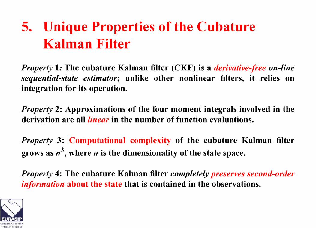
5. Unique Properties of the CubaKalman Filter

Property 1: The cubature Kalman filter (CKF) is a derisequential-state estimator; unlike other nonlinear filintegration for its operation.

Property 2: Approximations of the four moment integrderivation are all linear in the number of function evalu

Property 3: Computational complexity of the cubatu

grows as n3, where n is the dimensionality of the state s

Property 4: The cubature Kalman filter completely presinformation about the state that is contained in the obse

16

stitution of thee prior is known

properties of theg for improved

st known directming all other

blem


Property 5: Regularization is built into the concubature Kalman filter by virtue of the fast that thto play a role equivalent to regularization.

Property 6: The cubature Kalman filter inheritslinear Kalman filter, including square-root filterinaccuracy and reliability.

Property 7: The cubature Kalman filter is the closeapproximation to the Bayesian filter, outperfornonlinear filters in a Gaussian environment:

It eases the curse-of-dimensionality probut, by itself, does not overcome it.

17

uous-

te-estimationybridized:

l is described in is different.


6. Cubature Filtering for ContinDiscrete Nonlinear Systems

This second class of nonlinear filters deals with staproblems whose state-space models are naturally h

(i) Continuous-time state (process) sub-model.

(ii) Discrete-time measurement sub-model.

In mathematical terms, the measurement sub-modethe same way as in Eq. (2), but the state sub-model

18

rt to stochastic equation:

(6)


State (process) Sub-model

To describe the process sub-model, we have to resodifferential-equation theory, exemplified by the Ito

where xt is the unknown state at time t,

a(x,t) is some unknown function

Q is the so-called diffusion matrix

wt is the standard Gaussian noise

dxt

dt-------- a x t,( ) Qwt+=

19

ocess sub-model

ethod or


Discretization of the Process Equation

With recursive digital computation in mind, the prwould have to be discretized in the time domain.

The discretization can be performed using:

(i) Numerical methods, exemplified by the Euler mRunge-Kutta method.

(ii) The Ito-Taylor expansion of order 1.5.

20

y proceeding inubature Kalman

eveloped a newSCKF whose

f cubaturedictedof the


Cost-Reduced Square-root CKF

Having performed the discretization, we find that bthe same way as before, the resulting square-root cfilter (SCKF) is computationally expensive.

To overcome this practical difficulty, we have dnonlinear filter, named the cost-reduceddistinguishing feature is summarized as follows:

The modified time-update propagates a set opoints without having to estimate the premean and covariance at every time-step

filtering computation.

21

uare-root

near Systems:


Reference II

For mathematical derivation of the cost-reduced sqcubature Kalman filter, refer to

I. Arasaratnam, S. Haykin, and T. Hurd“Cubature Filtering for Continuous-Discrete NonliTheory with an Application to Tracking”

to be submitted for publication.

22

les.

crete extensionthe hidden stateis too difficult


7. Practical Applications

(i) Aerospace ApplicationsTracking of aircraft, satellites and guided missi

(ii) Training of Recurrent Neural Networks

Simply stated:

The Cubature Kalman filter and its continuous-disprovide new signal-processing tools for estimating of a nonlinear dynamic system whose nonlinearity for the traditional use of extended Kalman filters.

23

e, assumedhe origin.

urbed by additive

e turning force

havior near the performance of


8. Example I: Tracking aManoeuvring Ship

Problem statement:

Track a ship moving in an area bounded by a shore linto be a circular disc of known radius and centered at t

• The ship’s motion is modelled by a constant velocity pertwhite Gaussian noise.

• When the ship tries to drift outside the shoreline, a gentlpushes it back towards the origin.

• The model is interesting in that it exhibits a nonlinear beshoreline, thereby providing a good test for assessing thedifferent nonlinear filters.

24

(7)

(8)

(9)

(10)


• Dynamic State-space Model (Kushner and Budhiraja, 2000)

• where

xt ξ tη f 1 xt( ) f 2 xt( )[ ]T

Qtβt+=

rk

θk

ξk2 ηk

2+

ηk

ξk------

1–

tan

wk+=

f 1 x( )Kξ–

ξ2 η2+

----------------------, ξ2 η2+ r and ξξ ηη 0;≥+≥

0, otherwise

=

f 2 x( )Kη–

ξ2 η2+

----------------------, ξ2 η2+ r and ξξ ηη 0;≥+≥

0, otherwise

=

25

t interval to

d

ce, P0|0 = 10I4

σθ0.5π180-----------=


Tracking Example (continued)

• Use the Euler method with 5 steps for each measuremennumerically integrate Eq. (7)

• Data:

- Radius of the disk-shape shore, r = 5 units

- Gaussian process noise intensity, Q = 0.01

- Gaussian measurement noise parameters, σr = 0.01 an

- Estimated initial state, and covarian

where I4 is four-dimensional identity matrix.

- Radar scans = 1000/Monte Carlo run

- 50 independent Monte Carlo runs

x0 0 1 1 1 1, , ,[ ] T=

26
Motion of the ship.

Figure 1: I - initial point, F - final point, ★ - Radar location

−5 0 5−5

0

5

η

ε

I

F

27

800


Performance Comparison: RMSE in position

Figure 2: dashed red-Particle filter (PF) (1000 particles),thin blue-Central-difference Kalman filter (CDKF)

dark black-Cubature Kalman filter (CKF)

300 400 500 600 700

0

0.4

0.8

1.2R

MS

Epo

s

Time, k

28

ark black- CKF

800


Performance Comparison” RMSE in velocity

Figure 3: dashed red- PF (1000 particles), thin blue- CDKF, d

300 400 500 600 700

0.2

0.4

0.6

0.8

1

RM

SE

vel

Time, k

29

ent

(11)

r of degrees ofl value of xt

dimension.


9. Example II: Training a RecurrNeural Network

Mackey-Glass Attractor

where t denotes continuous time,a = 0.2b = 0.1∆t = 30

The Mackey-Glass attractor has an infinite numbefreedom because we require knowledge of the initiaacross a continuous-time interval.

Yet, it behaves like a strange attractor with a finite

ddt-----xt bxt

axt-∆t

1 xt-∆t+--------------------+=

30

ing the autonomoustractor

0


Figure 4: Ensemble-averaged cumulative absolute error curves durprediction phase of dynamic reconstruction of the Mackey-Glass at

0 20 40 60 80 100

5

10

15

20

25

Cum

ulat

ive

abs

olut

e er

ror

prediction time step

EKFCDKFCKF

31

cy filter (1961)ar discrete-timeents,rior (MAP)

an filter (and itsthe cost-reducedn Reference II,nlinear discrete

pectively, beingapproximations


10. Concluding Remarks

The classical Kalman filter (1960) and Kalman-Buprovide optimal estimates of the hidden state of lineand continuous-time systems in Gaussian environmrespectively, being optimal in the maximum a postesense.

The two new nonlinear filters, the Cubature Kalmsquare-root version) described in Reference I andsquare-root cubature Kalman filter described iprovide optimal estimates of the hidden state of noand continuous-discrete (hybrid) systems, resoptimal in the sense that they are the closest directto the Bayesian filter in Gaussian environments.

32

er


The slides for this Webinare available

on my website

http://soma.mcmaster.ca

Documents

Cubature Filters - EURASIP · Webiner, CISDA Tutorial, Ottawa, July 2009 (Haykin) 1 Cubature Filters: New Generation of Nonlinear Filters that will Impact the Literature