AAS 15-423

GENERALIZED GAUSSIAN CUBATURE FOR NONLINEARFILTERING

Richard Linares∗

Los Alamos National Laboratory, Los Alamos, NM, 87544John L. Crassidis†

University at Buffalo, State University of New York, Amherst, NY, 14260-4400

A novel method for nonlinear filtering based on a generalizedGaussian cubatureapproach is shown. Specifically, a new point-based nonlinear filter is developedwhich is not based on one-dimensional quadrature rules, butrather uses multi-dimensional cubature rules for Gaussian distributions. The new generalized Gaus-sian cubature filter is not in general limited to odd-order degrees of accuracy, andprovides a wider range of order of accuracy. The method requires the solution of aset of nonlinear equations for finding optimal cubature points, but these equationsare only required to be solved once for each state dimensional and order of accu-racy. This rule is also extended to anisotropic cases where the order of accuracy isnot isotropic in dimension. This method allows for tuning ofthe cubature rules todevelop problem specific rules that are optimal for the givenproblem. The general-ized Gaussian cubature filter is applied to benchmark problems in astrodynamics,and it is compared against existing nonlinear filtering methods.

INTRODUCTION

Sequential state estimation has been successfully appliedto number of problems in many dis-ciplines including; aircraft tracking, satellite orbit determination,1 spacecraft attitude determine,2,3

and many others.4,5,6,7 The main goal of sequential state estimation is to use measurements of thesystem of interest along with dynamic model to determine an estimate of current state and somemeasure of error in this estimate. The Bayesian framework provides a mechanism to completelydetermine the probability space of the system state but the solution is not in general solvable fornonlinear systems. Several approach

Optimal integration approximation theory in one dimensionis well-known, and many rules havebeen developed for different weighting functions and integration domains. In this work two distinc-tions are made; one between rules in one dimension and rules in multiple dimensions, and anotherbetween whether rules that are based on classical types of theory or more generalized forms. Inte-gration rules in one dimension are referred to as “quadrature rules” and integration rules in multidimensions are referred to as “cubature rules.” Likewise integration rules are referred to as classicalor generalized defined by their individual based theory.

∗Director’s Postdoctoral Fellow, Intelligence and Space Research. Email: linares@lanl.gov.†CUBRC Professor in Space Situational Awareness, Department of Mechanical & Aerospace Engineering. Email:johnc@buffalo.edu.

1

The Gaussian quadratures rules in particular involve the optimal integration of polynomials withthe minimum number of nodes. It is well-known how to construct Gaussian quadratures for one-dimensional integrals. Rules based on orthogonal polynomials are also well-known, and are referredto as Classical Gaussian Quadrature (CGQ) in this work. Recently a different class of quadraturerules has been developed that is not based on orthogonal polynomials, but rather on the integration ofgeneral classes of functions. These rules are referred to asGeneralize Gaussian Quadrature (GGQ)in this work.8

For higher-dimensional problems optimal integration rules are very important. Integrals for di-mensions greater than one still remain a challenge. The moststraightforward way to constructthese rules with tensor products of one-dimensional Classical Gaussian Cubature (CGC) rules.9,10,11

These tensor products produce rules that are far from optimal, and require much more nodes thanneeded to achieve a pre-selected desirable precision. In particular the number of nodes increasesrapidly with dimension, making these rules un-usable for dimensions greater than 20. This currentwork investigates a technique called generalized Gaussiancubature where the rules are constructedto integrate a set of function exactly. Also, this work develops an approach to form generalizedGaussian cubature rules for Gaussian mixture distributions.

PROBLEM STATEMENT

For Gaussian nonlinear filters the key computational challenge is evaluating Gaussian integralsof the following form:

I(g) =∫

Rd

g(x)N (x|µ, P ) dx (1)

wherex ∈ Rd, g : Rd → R

1, andN (x|µ, P ) denotes a multivariate normal probability densityfunction for x with mean and covarianceµ andP , respectively. The sigma-point filtering andsmoothing methods in general can be viewed as methods which approximate the integral in Eq. (1)as

∫

Rd

g(x)N (x|µ, P ) dx ≈m∑

i=1

Wig(xi) (2)

whereWi andxi are predefined weights and sigma points, respectively. The Gaussian integral hasa solution in general using a change of variables, called stochastic decoupling, where sigma-pointsare developed to solve the following integral:

∫

Rd

g(η)N (η|0, I) dη ≈m∑

i=1

Wig(ηi) (3)

whereg = g(µ+√Pη) andP =

√P√P

T. Sigma-point methods differ in the selection of sigma-

points,η, and weights,Wi, to solve the integral in Eq. (1). In general the functiong can take on anyform. Therefore sigma-point methods are designed with the goal to be exact, and/or accurate for aclass of functions with the hope thatg is well approximated by this class.

Typically the class of functions considered are polynomialfunctions of several variables. Forthe purpose of this work the order of the multi-dimensional polynomials will be defined by its themonomial with the largest multi-indexL1 norm. The multi-index is denoted byα = (α1, . . . , αd),where eachαi is the order ofith variable in a given monomial. Then for a givenα the set of variablesx monomial in variablesx1, . . . , xn of indexα is given by

xα = (xα1

1 . . . xαd

d ) (4)

2

The number|α| =∑di=1 αi is then called the degree ofxα and the order of a polynomial in multiple

dimensions is determined by its highest degree monomial. The number of polynomial functions ind variables of degree less thanℓ is given by

Nℓ =(ℓ+ d)!

ℓ!d!(5)

The number of polynomials of degree greater thanℓ grows rapidly with dimension. This rapidgrowth is referred to the “curse of dimensionality.” In the following sections nonlinear Bayesianfilters based on Gaussian assumptions will be discussed. Tensor product and sparse gird tensorproduct cubature approximations to Eq. (1) will be shown. This will followed by a new generalizedGaussian cubature approach.

NONLINEAR GAUSSIAN FILTERING

In the general nonlinear filtering problem the goal is to determine an estimate of the state vectorx from observationsy, where the following dynamic and observation models are given:

xk = f(xk−1) +wk (6a)

yk = h(xk) + vk (6b)

wherewk andvk are zero-mean Gaussian noise processes with covariancesQk = EwkwTk and

Rk = EvkvTk , respectively. Sequential Bayesian state estimation usesthe a priorp(xk|y1:k−1)

(state uncertainty based on previous measurements) and thelikelihood p(yk|xk) (uncertainty basedon measurements) to calculate the posterior probability density function (pdf) of the state condi-tioned on the current measurements through

p(xk|y1:k) =p(yk|xk)p(xk|y1:k−1)

∫

p(yk|xk)p(xk|y1:k−1)dxk

(7)

In between measurements the conditional pdfp(xk|y1:k−1) is found using the Chapman-Kolmogorovequation:

p(xk|y1:k−1) =

∫

p(xk|xk−1)p(xk−1|y1:k−1)dxk−1 (8)

The nonlinear filtering problem given in Eq. (6) can be solved with Eq. (7) and Eq. (8), but ingeneral this problem is difficult to solve. Therefore, approximate Gaussian-based filters are of-ten used. In the Gaussian filtering approach the likelihood and transition pdfs are assumed to bep(xk|xk−1) = N (xk − f (xk−1) ; 0, Qk) andp(yk|xk) = N (yk − h (xk) ; 0, Rk), respectively.Then the nonlinear filter problem becomes estimating pre-update and post-update means and co-variances (xk|k−1, Pk|k−1 andxk|k, Pk|k, respectively). The pre-update mean and covarianceis found via propagating the state and covariance from the previous time-step to the current time-step, which is given by

xk|k−1 =

∫

Rd

f(xk−1)N(

xk−1; xk−1|k−1, Pk−1|k−1

)

dxk−1 (9a)

Pk|k−1 =

∫

Rd

f(xk−1)f(xk−1)TN

(

xk−1; xk−1|k−1, Pk−1|k−1

)

dxk−1 − xk|k−1xTk|k−1 +Qk

(9b)

3

Then given measurements, the post-update mean and covariance equations are given by

xk|k = xk|k−1 + Lk

[

yk − hk(xk|k−1)]

(10a)

Pk|k = Pk|k−1 − LkPTxy (10b)

where these equations follow the Gaussian filtering assumptions, and therefore have the Kalmanfilter structure. The terms in Eq. (10) are calculated as follows

Lk = Pxy (Rk + Pyy)−1 (11a)

yk =

∫

Rd

h (xk)N(

xk; xk|k−1, Pk|k−1

)

dxk (11b)

Pxy =

∫

Rd

(

xk − xk|k−1

)

(h(xk)− yk)T N

(

xk; xk|k−1, Pk|k−1

)

dxk (11c)

Pxx =

∫

Rd

(h(xk)− yk) (h(xk)− yk)T N

(

xk; xk|k−1, Pk|k−1

)

dxk (11d)

Finally, all the integrals in Eqs. (9), (10), and (11) can be determined by solving the integral inEq. (3). This paper proposes an improved solution to nonlinear filtering by improving the solutionof Eq. (3) with the method discussed in the next section.

Tensor Product Cubature

The most straightforward way of developing cubature rules is using tensor products of one-dimensional Gaussian quadrature rules. Tensor Product Cubature (TPC) rules can be derived forEq. (1) by noting thatN (η;0, I) = N (η1; 0, 1) · · · N (ηd|; 0 , 1), and the integral can be writtenas

∫

Rd

g(η)N (η; 0, I) dη =

∫

RN (η1; 0, 1) · · ·

∫

RN (η2; 0, 1)

∫

Rg(η)N (η1; 0, 1) dη1 dη2 · · · dηd

(12)

where the integral above allows for a telescoping evaluation for the integral, and one-dimensionalquadratures rules can be used for each of theηi integrals. Then the multidimensional integral inEq. (1) can be approximated using the tensor products of one-dimensional CGQ rules.3 Each inte-gral in Eq. (12) can be written as

∫

R1

g(ηj)N (ηj ; 0, 1) dηj =

m∑

i=1

g(ηij)Wij (13)

where the one-dimensional nodesηij and weightsW ij are from one of the several known one-

dimensional rules. Also,m denotes the number of points for the chosen level of accuracy. Theserules include Clenshaw-Curtis, Gauss-Patterson, Gauss-Hermite, Gauss-Legendre, Gauss-Laguerre,generalized Gauss-Laguerre, and Gauss-Jacobi. Each of these rules is a CGQ for a given weightfunction contained in the integral and the domain of the integral. In other words each rule is optimalfor a given form of the integral in Eq. (13).

Using the rule in Eq. (13), multidimensional rules are constructed with tensor products of theone-dimensional rules. Each one-dimensional rule is exactfor polynomials of degree less than or

4

equal to2mj −1, wheremj is the number of points used for the rule in thejth dimension. Differentrules may be used along each dimension and therefore the index α. The multi-index is then givenby α = (α1, · · ·αn), which is used to define the accuracy level along each dimension. The tensorproduct cubature rule is then defined by

I(g) ≈α1∑

i1=1

· · ·αn∑

in=1

g(ηij , )(wi1j ⊗ · · · ⊗ win

j ) (14)

The total number of cubature points required for the rule in Eq. (14) is given by the product of eachone-dimensional quadrature rule:

NTPC =

d∏

i=1

α(i) (15)

When the same level of accuracy is used for each dimension, the number of points for the tensorproduct quadrature rule is given by

NTPC = md (16)

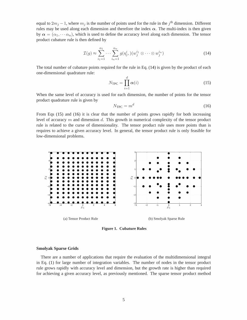
From Eqs (15) and (16) it is clear that the number of points grows rapidly for both increasinglevel of accuracym and dimensiond. This growth in numerical complexity of the tensor productrule is related to the curse of dimensionality. The tensor product rule uses more points than isrequires to achieve a given accuracy level. In general, the tensor product rule is only feasible forlow-dimensional problems.

−6 −4 −2 0 2 4 6−6

−4

−2

0

2

4

6

x1

x2

(a) Tensor Product Rule

−3 −2 −1 0 1 2 3−3

−2

−1

0

1

2

3

x1

x2

(b) Smolyak Sparse Rule

Figure 1. Cubature Rules

Smolyak Sparse Grids

There are a number of applications that require the evaluation of the multidimensional integralin Eq. (1) for large number of integration variables. The number of nodes in the tensor productrule grows rapidly with accuracy level and dimension, but the growth rate is higher than requiredfor achieving a given accuracy level, as previously mentioned. The sparse tensor product method

5

is a popular cubature method which is more efficient than tensor product-based rules. One sparsetensor product method is the Sparse Grid Cubature (SGC) method, which was first introduced bySmolyak10 and further developed by others. These methods reduce the number of cubature pointsdrastically while maintaining the desired accuracy level.

The Smolyak isotropic formulas will now be described, following from a description in Ref.10.The Smolyak isotropic formula operator is denoted byQ

(N)ℓ , whereℓ is a level that is independent

of dimensionN . The Smolyak formulas reduce the number of nodes by only using tensor productswith relatively small number of points. The Smolyak formulas are linear combinations of the prod-uct formulas that limit the growth of the number of nodes by limiting tensor products which resultin large number of points. Another key property is in the definition of difference formulas:

∆i = Ui − Ui−1 (17)

with U0 = 0. For i ≥ 1 the quadratureUi can be written as

Ui =l∑

i=1

∆i (18)

Theℓth degree quadrature can be written as the sum of difference formulas. The use of the differenceformulas simplifies the sparse cubature formulas greatly for multidimensional cases. The isotropicSmolyak quadrature formula is given by

Q(N)ℓ =

∑

|α|≤ℓ+n

(∆α1 ⊗ · · · ⊗∆αn) (19)

Note that|α| = α1 + · · · + αn. Equivalently, the formula in Eq. (19) can be written as

Q(N)ℓ =

∑

ℓ+1≤|α|≤ℓ+N

(−1)w+d−|α|

(

d− 1w + d− |α|

)

(Uα1 ⊗ · · · ⊗ Uαn) (20)

The form of Eq. (20) is also valid for the tensor product cubature rule in Eq. (12). This rule can bewritten by

Q(N)ℓ =

∑

max |α|≤ℓ

(Uα1 ⊗ · · · ⊗ Uαn) , max |α| ≡ maxℓ1, . . . , ℓN (21)

The difference between the full tensor product rules and thesparse tensor product rules is the indexα used in the summation. The full tensor rules sum over a hypercube of a multi-index space, andconsider much more terms than are necessary for the given order accuracy, whereas the sparse rulessum over a simplex of terms less than or equal to the desired order. The simplex used for thesparse rules is defined by|α| ≤ ℓ. An example of a tensor rule and sparse rule is shown in Figure1. Here one can see that the tensor rule uses far more points than necessary, whereas the sparserule tends to focus the points more in areas of importance. Sparse rules require nesting of one-dimensional rules, and are limited by the properties of these one-dimensional rules. For example,one-dimensional rules can achieve an order of accuracy thatis 2m− 1, which means that only odd-order orders of accuracy can be achieved. The work in this papers derives a general approach fordeveloping cubature rules that reduces the number of nodes used, thereby controlling the growth ofnodes with increasing dimension. An adaptive multi-index space can be used to optimize the rulefor the problem to be solved.

6

−2 −1.5 −1 −0.5 0 0.5 1 1.5 2−2

−1.5

−1

−0.5

0

0.5

1

1.5

2

x

y

(a) Tensor GC Order 3

−2 −1.5 −1 −0.5 0 0.5 1 1.5 2−2

−1.5

−1

−0.5

0

0.5

1

1.5

2

x

y

(b) Tensor GC Order 5

−2.5 −2 −1.5 −1 −0.5 0 0.5 1 1.5 2 2.5−2.5

−2

−1.5

−1

−0.5

0

0.5

1

1.5

2

2.5

x

y

(c) Tensor GC Order 7

−1 −0.5 0 0.5 1

−1

−0.5

0

0.5

1

x

y

(d) Sparse GC Order 3

−2 −1.5 −1 −0.5 0 0.5 1 1.5 2−2

−1.5

−1

−0.5

0

0.5

1

1.5

2

x

y

(e) Sparse GC Order 5

−2.5 −2 −1.5 −1 −0.5 0 0.5 1 1.5 2 2.5−2.5

−2

−1.5

−1

−0.5

0

0.5

1

1.5

2

2.5

x

y

(f) Sparse GC Order 7

−1.5 −1 −0.5 0 0.5 1 1.5−1.5

−1

−0.5

0

0.5

1

1.5

x

y

(g) GGC Order 3

−2 −1.5 −1 −0.5 0 0.5 1 1.5 2−2

−1.5

−1

−0.5

0

0.5

1

1.5

2

x

y

(h) GGC Order 5

−3 −2 −1 0 1 2 3−3

−2

−1

0

1

2

3

x

y

(i) GGC Order 7

−2 −1.5 −1 −0.5 0 0.5 1 1.5 2−2

−1.5

−1

−0.5

0

0.5

1

1.5

2

x

y

(j) UKF

Figure 2. Cubature Points vs Order in 2 Dimensions

7

GENERALIZED GAUSSIAN CUBATURE

The extension of the classical theory of orthogonal polynomials to multiple dimensions is far fromcomplete. By far the clearest approach seems to be extendingGGQ to multidimensional functions.Throughout this work this extension will be called Generalize Gaussian Cubature (GGC). The GGCfor multidimensional cases is designed to evaluate the following multidimensional integral:

∫

Ωf(x)w(x)dx ≈

m∑

i=1

Wif(xi) (22)

whereWi andxi are the multidimensional GGC weights and nodes, respectively, f is an integranddefined overΩ, andw is the pdf weighting function. As in the one-dimensional GGQthe GGC isdesigned so that Eq. (22) is exact for all functions for a pre-selected set. Classical choices of thepre-selected set of functions include polynomials up to a certain degree, trigonometric functions,and basis functions of a particular function space defined onΩ. Then the GGQ equation is writtenas

∫

Ω ϕ1 (x)w(x)dx∫

Ω ϕ2 (x)w(x)dx...

∫

Ω ϕm (x)w(x)dx

=

ϕ1 (x1) ϕ1 (x2) . . . ϕ1 (xn)ϕ2 (x1) ϕ2 (x2) . . . ϕ2 (xn)

...ϕN (x1) ϕN (x2) . . . ϕN (xn)

W1

W2...

Wm

(23)

whereϕi (x) are the pre-selected functions andN is the function of functions used. Not that if thefunctions are selected toℓ order polynomials ind variable thenN = Nℓ. The equation above canbe casted into a minimization problem to determine the weights and nodes as follows

J =

N∑

j

(

m∑

i

Wiϕj (xi)−∫

Ωϕj (x)w(x)dx

)2

(24)

This work focuses on polynomials as the pre-selected set of functions so thatϕ1 (x) are poly-nomial functions. From Eq. (23) it is seen that this system of equations hasm multidimensionalintegrals that must be solved. Solving these integrals for high-dimensional space can be arduous.To simplify the process this work will focus on multi-dimensional Gaussian distributions. The ben-efit of Gaussian distributions is that them multidimensional integrals in Eq. (23) have closed-formsolutions.

The GGC for a Gaussian distribution can take a simple form if theϕj (x) functions are chosen tobe Hermite polynomials for a multidimensional Gaussian distribution. The orthogonal polynomialfor a Gaussian distribution can be written as a product of one-dimensional Hermite polynomials. Todetermine these polynomials, a coordinate transformationis used to covert the Gaussian distribu-tion into a product of unit variate normal distributions. Specifically, given the following Gaussiandistribution

p(x) = N (x; µ, P ) (25)

the square-root factorS is computed fromP (using a Cholesky factorization), and the followingtransformation is defined:

u = S−1(µ− x) (26)

8

Then the pdf ofu can be written as

p(u) = N (u(1); 0, 1) · · · N (u(n); 0, 1) (27)

whereu(j) denotes thejth component ofu. Then the multidimensional orthogonal polynomials forvariableu is written as the following product of polynomials:

Pα(u) =

d∏

j=1

Hαj(u(j)) (28)

where the subscript of the Hermite polynomial denotes the order of the one-dimensional polynomial.The multidimensional orthogonal polynomial is a product ofunivariate Hermite polynomials, givenby

Hn(x) = (−1)n exp(

x2/2) dn

dxnexp(−x2/2) (29)

whereHn(x) is the orthogonal with respect to a one-dimensional unit-variate zero-mean Gaussiandistribution. The mean ofHn(x) is given by

EHn(x) = µn (30)

whereµ is the mean of the Gaussian weight function used to definedHn(x). From the defini-tion in Eq. (26) it is noted thatu has zero mean, and thereforeEHn(uj) = 0 for n = 0 andEHn(u0) = 1 for n 6= 0. Define the following vectorL ≡ [L1 . . . Lm]T , where

Lj =

∫

ΩPαj

(u)p(u)du

=

∫ ∞

−∞. . .

∫ ∞

−∞Hα1

(u1) . . . Hαn(un)N (u1; 0, 1) . . .N (un; 0, 1)du1 . . . duj

=

∫ ∞

−∞Hα1

(u1)N (u1; 0, 1)du1 . . .

∫ ∞

−∞Hαn(un)N (u1; 0, 1)dun

=

d∏

i=1

EHαi(ui)

(31)

Form Eq. (31) it can be seen that if|αj | 6= 0 thenLj = 0. This simplifies the problem greatlysince theN -dimensional integrals involved in Eq. (31) do not need to be calculated. Therefore, thefollowing equation is true:

L =

∫

Ω Pα1(u)p(u)du

∫

Ω Pα2(u)p(u)du

...∫

Ω Pαn(u)p(u)du

=

10...0

(32)

Equation (23) can be written in matrix form by defining the following matrix:

M ≡

Pα1(u1) Pα1

(u2) . . . Pα1(un)

Pα2(u1) Pα2

(u2) . . . Pα2(un)

...Pαn(u1) Pαn(u2) . . . Pαn(un)

(33)

9

Finding the GGC solution for the system of equations given inEq. (23) involves finding bothw ≡[W1, . . . , Wm]T andz ≡ [uT

1 , . . . , uTm]T , which are combined into the vector defined byΘ ≡

[wT zT ]T . The cubature rule is then given by the solution to the following minimization problem,ΘGGC = minΘ J(Θ), where the objective function is given by

J(Θ) =1

2[L−M(z)w]T [L−M(z)w] (34)

Then the Jacobian matrix is calculated asδJ(Θ)δΘ

= − [M(z) Φ]T [L−M(z)w], whereΦ is givenby

Φ =

w1ϕ′

1(u1) . . . wnϕ′

1(um)...

...w1ϕ

′

m(u1) . . . wnϕ′

m(um)

(35)

Thenϕ′

j(u) terms are calculated by

ϕ′

j(x) =(

H′

αj(u1(1)) . . . Hαj

(u1(d)) . . . Hαj(u1(1)) . . . H

′

αj(u1(d))

)

(36)

From the properties of the Hermite polynomials,H′

n(x) has a simple expression given by

H′

n(x) = nHn−1(x) (37)

Then the minimization problem can be rewritten as follows

J(Θ) = wTK(z, z)w − 2wTMTL+ 1 (38)

whereK(z, z) ≡ MTM . Then the first-order optimality condition can be written as

∂J(Θ)

∂w=K(z, z)w −MTL = 0 (39a)

∂J(Θ)

∂z=ΦTMw = 0 (39b)

whereMTL is a vector of ones for Hermite polynomials. From Eq. (39) it can be noted thatif L = M(z)w the first-order optimality conditions are meet. Using the first-order optimalitycondition given in Eq. (39) the weight vector can be solved by

w = K(z, z)−1MTL (40)

Then substituting Eq. (40) into Eq. (38), the objective function can be written as

J(Θ) = 1− LTMK(z, z)−1MTL (41)

Equation (41) reduces the dimensionality of the minimization problem byn parameters. Then usingEqs (32) and (33) the objective function in Eq. (41) can be minimized, and a solution for the GGCcan be found. This minimization does not require the evaluation of theN -dimensional integralsin L, and can be vectorized for rapid evaluation of the objectivefunction and the Jacobian. WithJacobian information efficient Newton-based methods can beused. These methods can be used tofind Gaussian distribution cubature rules for different dimensions and order. More importantly, thedefinition ofα can used to find adaptive sparse rules to limit the growth of the number of points,and temper the curse of dimensionality.

10

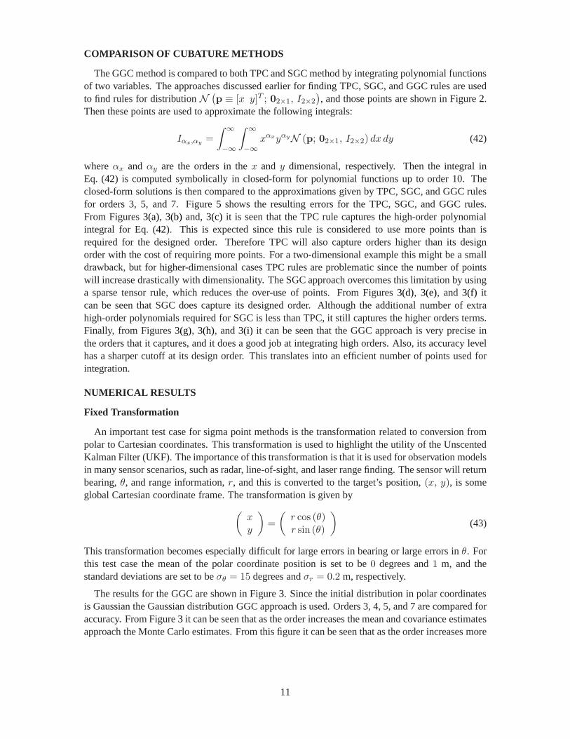
COMPARISON OF CUBATURE METHODS

The GGC method is compared to both TPC and SGC method by integrating polynomial functionsof two variables. The approaches discussed earlier for finding TPC, SGC, and GGC rules are usedto find rules for distributionN

(

p ≡ [x y]T ; 02×1, I2×2

)

, and those points are shown in Figure2.Then these points are used to approximate the following integrals:

Iαx,αy =

∫ ∞

−∞

∫ ∞

−∞xαxyαyN (p; 02×1, I2×2) dx dy (42)

whereαx andαy are the orders in thex and y dimensional, respectively. Then the integral inEq. (42) is computed symbolically in closed-form for polynomial functions up to order 10. Theclosed-form solutions is then compared to the approximations given by TPC, SGC, and GGC rulesfor orders 3, 5, and 7. Figure5 shows the resulting errors for the TPC, SGC, and GGC rules.From Figures3(a), 3(b) and,3(c) it is seen that the TPC rule captures the high-order polynomialintegral for Eq. (42). This is expected since this rule is considered to use more points than isrequired for the designed order. Therefore TPC will also capture orders higher than its designorder with the cost of requiring more points. For a two-dimensional example this might be a smalldrawback, but for higher-dimensional cases TPC rules are problematic since the number of pointswill increase drastically with dimensionality. The SGC approach overcomes this limitation by usinga sparse tensor rule, which reduces the over-use of points. From Figures3(d), 3(e), and3(f) itcan be seen that SGC does capture its designed order. Although the additional number of extrahigh-order polynomials required for SGC is less than TPC, itstill captures the higher orders terms.Finally, from Figures3(g), 3(h), and3(i) it can be seen that the GGC approach is very precise inthe orders that it captures, and it does a good job at integrating high orders. Also, its accuracy levelhas a sharper cutoff at its design order. This translates into an efficient number of points used forintegration.

NUMERICAL RESULTS

Fixed Transformation

An important test case for sigma point methods is the transformation related to conversion frompolar to Cartesian coordinates. This transformation is used to highlight the utility of the UnscentedKalman Filter (UKF). The importance of this transformationis that it is used for observation modelsin many sensor scenarios, such as radar, line-of-sight, andlaser range finding. The sensor will returnbearing,θ, and range information,r, and this is converted to the target’s position,(x, y), is someglobal Cartesian coordinate frame. The transformation is given by

(

xy

)

=

(

r cos (θ)r sin (θ)

)

(43)

This transformation becomes especially difficult for largeerrors in bearing or large errors inθ. Forthis test case the mean of the polar coordinate position is set to be0 degrees and1 m, and thestandard deviations are set to beσθ = 15 degrees andσr = 0.2 m, respectively.

The results for the GGC are shown in Figure3. Since the initial distribution in polar coordinatesis Gaussian the Gaussian distribution GGC approach is used.Orders 3, 4, 5, and 7 are compared foraccuracy. From Figure3 it can be seen that as the order increases the mean and covariance estimatesapproach the Monte Carlo estimates. From this figure it can beseen that as the order increases more

11

0 5 10 150

5

10

15

x order

yorder

−14

−12

−10

−8

−6

−4

−2

0

2

4

(a) Tensor GC Order 3

0 5 10 150

5

10

15

x order

yorder

−14

−12

−10

−8

−6

−4

−2

0

2

4

(b) Tensor GC Order 5

0 5 10 150

5

10

15

x order

yorder

−14

−12

−10

−8

−6

−4

−2

0

2

4

(c) Tensor GC Order 7

0 5 10 150

5

10

15

x order

yorder

−14

−12

−10

−8

−6

−4

−2

0

2

4

(d) Sparse GC Order 3

0 5 10 150

5

10

15

x order

yorder

−14

−12

−10

−8

−6

−4

−2

0

2

4

(e) Sparse GC Order 5

0 5 10 150

5

10

15

x order

yorder

−14

−12

−10

−8

−6

−4

−2

0

2

4

(f) Sparse GC Order 7

0 5 10 150

5

10

15

x order

yorder

−14

−12

−10

−8

−6

−4

−2

0

2

(g) GGC Order 3

0 5 10 150

5

10

15

x order

yorder

−14

−12

−10

−8

−6

−4

−2

0

2

4

(h) GGC Order 5

0 5 10 150

5

10

15

x order

yorder

−14

−12

−10

−8

−6

−4

−2

0

2

(i) GGC Order 7

0 5 10 150

5

10

15

x order

yorder

−14

−12

−10

−8

−6

−4

−2

0

2

(j) UKF

Figure 3. Polynomial Error vs Order in 2 Dimensions

12

−0.8 −0.6 −0.4 −0.2 0 0.2 0.4 0.6 0.8 1

0.65

0.7

0.75

0.8

0.85

0.9

0.95

1

1.05

1.1

xy

Figure 4. Monte Carlo Points for Polar to Cartesian Coordinates Transformation Example

nodes are used in the GGC approach, which captures the “banana” shape of the Monte Carlo pointsmore closely.

Uncertainty Propagation: Nonlinear Spring Mass System

To test the performance of the new GGC rules for propagation of uncertainty through a dynamicsystem, a simple nonlinear two-dimensional example is used. This example models a nonlinearspring-mass system with a nonlinear friction term. The system dynamics for this simple exampleare written as

x1 = x2 (44a)

x2 = κx1 + εx31 + bx2 (44b)

The parametersε, κ, andb affect the system behavior to varying degrees. For this simulation thesevalues are selected to beε = 0.1, κ = 1e4/2π, andb = 0.05. The simulation time considered is 200seconds with a sampling interval 0.1 seconds. The initial state is given byx0 = [0.2 0.3]T . Theinitial state covariance is given byP0 = diag([0.12 0.12]). Monte Carlo simulations are conductedto test the GGC approaches. The Monte Carlo samples are takenfrom the initial distribution, and1,000 samples are used in the comparisons.

The errors in the meansx1 andx2 that are computed for the different order GGC are comparedto the means calculated from the Monte Carlo samples at each time step. These errors are shownin Figures7(a)and7(b) for thex1 andx2 means, respectively. The norm of the state error is alsocalculated and is shown in Figure7(c). From these figures it can seen that as the order increasesthe approximation of the mean is improved. During the initial portion of the simulation the errorsare large for all the models since the nonlinear spring is fluxing greatly (as seen in Figure6) but thehigher-order GGC still has better performance. As the energy dissipates the system fluctuation islower but the higher-order models still show better performance.

Example 1: Nonlinear Spring-Mass System

The first filtering example is a nonlinear spring-mass model with nonlinear measurements. Thenonlinear spring-mass model is the same as the one used in Eq.(44) to test the uncertainty propa-

13

−0.8 −0.6 −0.4 −0.2 0 0.2 0.4 0.6 0.8 1

0.7

0.8

0.9

1

1.1

1.2

1.3

MCMC CovMC MeanGC CovGC MeanGC Sigma

x

y

(a) Order 3

−0.8 −0.6 −0.4 −0.2 0 0.2 0.4 0.6 0.8 1

0.7

0.8

0.9

1

1.1

1.2

1.3

MCMC CovMC MeanGC CovGC MeanGC Sigma

x

y

(b) Order 4

−0.8 −0.6 −0.4 −0.2 0 0.2 0.4 0.6 0.8 1

0.7

0.8

0.9

1

1.1

1.2

1.3

MCMC CovMC MeanGC CovGC MeanGC Sigma

x

y

(c) Order 5

−0.8 −0.6 −0.4 −0.2 0 0.2 0.4 0.6 0.8 1

0.7

0.8

0.9

1

1.1

1.2

1.3

MCMC CovMC MeanGC CovGC MeanGC Sigma

x

y

(d) Order 7

Figure 5. Polar to Cartesian Coordinates Transformation Example

gation performance of the GGC approach. The state variablesarex1 andx2, which are the positionand velocity of the spring-mass system. The following measurement function is used:

yk = exp (x1k − c) + vk (45)

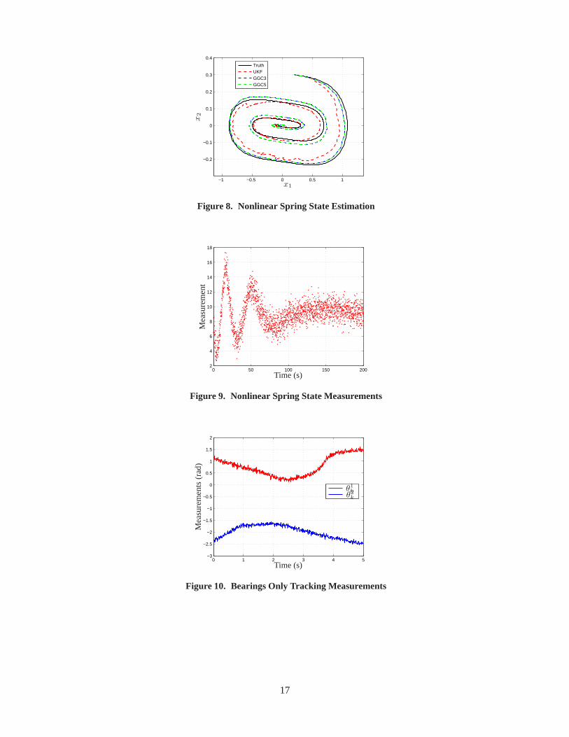
wherevk is the measurement noise, which is defined to bevk ∼ N (0, σ2), with σ = 20 andc = 3for the simulation example. The initial true state used for this example is given byx0 = [0.2 0.3]T .The initial state covariance is given byP0 = diag([0.12 0.12]) and the initial state estimate isx0 = [0.3 0.4]T . Measurements are sampled at 0.1 second intervals for a total of 200 secondsimulation time. The measurement for this simulation scenario is given in Figure9.

The state estimates for UKF, GGC order 3, and GGC 5 are shown inFigure8. From Figure8it can be seen that the UKF has the worst performance while theGGC method does a better job attracking the truth. All filters diverge initially, but the UKF has the largest divergence. Also the UKFtakes the longest amount of time to converge to the true state.

14

0 20 40 60 80 100−1

−0.5

0

0.5

1

1.5

0 20 40 60 80 100−0.4

−0.2

0

0.2

0.4

Time (min)

x1

x2

(a) True States

−1 −0.5 0 0.5 1 1.5−0.4

−0.3

−0.2

−0.1

0

0.1

0.2

0.3

x1

x2

(b) Phase Portrait

Figure 6. Numerical Integration Example Simulation Results

Example 2: Bearings Only Tracking

A classical filtering application in which a moving object istracked by measuring only the bear-ings (angles) of the object with respect to the position of the sensors is shown here. There is onemoving target in the scene and two angular sensors for tracking it. Solving this problem is important,because often more general multiple target tracking problems can be partitioned into sub-problems,in which single targets are tracked separately at a time. Thestate of the target at time stepk consistsof the position in two-dimensional Cartesian coordinatesxk andyk and the respective velocities.The state vector can be expressed as

xk =(

xk yk xk yk)T

(46)

The dynamics of the target is modeled as a linear, discretized Wiener velocity model given by

xk+1 =

1 0 ∆t 00 1 0 ∆t0 0 1 00 0 0 1

xk−1

yk−1

xk−1

yk−1

+ qk−1 (47)

whereqk−1 is Gaussian process noise with zero mean and covariance

Eqk−1qTk−1 =

13∆t3 0 1

2∆t2 0

0 13∆t3 0 1

2∆t2

12∆t2 0 ∆t 0

0 12∆t2 0 ∆t

q (48)

whereq is the spectral density of the noise, which is set toq = 0.1 in the simulations. The measure-ment model for sensori is defined as

θik = arctan

(

yk − siyyx − six

)

+ vik (49)

15

0 50 100 150 2000

0.2

0.4

0.6

0.8

1

1.2

1.4

GC3GC4GC5GC7

x1

Err

or

Time (s)

(a)x1 Error

0 50 100 150 2000

0.1

0.2

0.3

0.4

0.5

0.6

0.7

GC3GC4GC5GC7

x2

Err

or

Time (s)

(b) x2 Error

0 50 100 150 2000

0.2

0.4

0.6

0.8

1

1.2

1.4

GC3GC4GC5GC7

Nor

mx

Err

or

Time (s)

(c) Norm of x Error

Figure 7. Dynamic System Propagation Example

where(six, siy) is the position of sensori andvik ∼ N (0, σ2), with σ = 0.05 radians. Figure

10 shows a plot of a one realization of measurements in radians obtained from both sensors. Thesensors are placed at locations(s1x, s

1y) = (−1, −2) and(s2x, s

2y) = (1, 1).

From the figure it can be seen that since the velocity errors are large all the models divergeinitially. From Figure8 it can be seen that the UKF has the largest divergence while the GGCapproach has smaller divergence. Also, as the order increases in the GGC methods the divergenceinitially is less, and the filter does a better job tracking maneuvers.

Example 3: Attitude Estimation Example

This section discusses a simulation example that compares the performance of the GGC filter,UKF, and the EKF. The GGC uses the approach for representing the pdf as sigma points discussedearlier. Large initial errors are considered. It is important to note that with large initial errors the

16

−1 −0.5 0 0.5 1

−0.2

−0.1

0

0.1

0.2

0.3

0.4

TruthUKFGGC3GGC5

x1

x2

Figure 8. Nonlinear Spring State Estimation

0 50 100 150 2002

4

6

8

10

12

14

16

18

Mea

sure

men

t

Time (s)

Figure 9. Nonlinear Spring State Measurements

0 1 2 3 4 5−3

−2.5

−2

−1.5

−1

−0.5

0

0.5

1

1.5

2

θ1kθ2k

Mea

sure

men

ts(r

ad)

Time (s)

Figure 10. Bearings Only Tracking Measurements

17

−1 −0.5 0 0.5 1−2

−1.5

−1

−0.5

0

0.5

TruthUKFGGC3GGC5

x

y

Figure 11. Bearings Only Tracking Filtering Example

0 1 2 3 4 5 6 7 810

−3

10−2

10−1

100

101

102

103

EKFUKFGQF−3

Att

itude

Err

or(D

eg)

Time (Hr)

Figure 12. Attitude Error

attitude distribution becomes highly nonlinear.

The example shown here is taken directly from Ref.2. Attitude errors of−50, 50 and 160 degreesfor each axis, respectively, are added into the initial-condition attitude estimate. The initial attitudecovariance is set to (50 degrees)2 for each attitude component. The initialx- andz-axes estimatesfor the gyro biases are set to zero, however the initial y-axis bias estimate is 20 deg/hr. The initialbias covariance is set to (20 deg/hr)2 for each axis. The initial particles are drawn using a Gaussiandistribution with the aforementioned covariance matrices, which ensures that each filter is initializedin a consistent manner.

A plot of the norm of the attitude errors for this simulation case is shown in Figure12. The EKFdoes not converge for this case since the first-order approximation cannot adequately capture thelarge initial condition errors. The UKF does have better convergence properties than the EKF forthis case, however the GGC provides the best convergence performance. Both the EKF and the UKF

18

are more sensitive to the initial conditions than the GGC. The performance of the GGC is checkedby running the filter 100 times. It always converges and the statistics of the estimation results in the100 runs are almost identical.

CONCLUSIONS

This paper investigated a technique called generalized Gaussian cubature, where the rules areconstructed to integrate a set of functions exactly. Hermite and Sparse Tensor products approachesfor multi-dimensional integral were discussed. The generalized cubature approach was used to solvemulti-dimensional integrals of Gaussian distributions. The solution was simplified greatly by usingthe generalized cubature technique along with properties of Gaussian distributions. Additionally,the solution of nodes and weights for the generalized cubature of a Gaussian distribution was alsogreatly simplified by using the multi-dimensional Hermite polynomials. Cubatures were derived fora number of orders and dimensions and used for both uncertainty propagation and sequential stateestimation. Good results were shown with the new methods.

REFERENCES

[1] Kelecy, T. and Jah, M., “Analysis of High Area-to-Mass Ratio (HAMR) GEO Space Object Orbit De-termination and Prediction Performance: Initial Strategies to Recover and Predict HAMR GEO Trajec-tories with No A Priori Information,”Acta Astronautica, Vol. 69, 2011, pp. 551–558.

[2] Crassidis, J.L. and Markley, F.L., “Unscented Filtering for Spacecraft Attitude Estimation,”Journal ofGuidance, Control and Dynamics, Vol. 26, No. 4, July-Aug. 2003, pp. 536–542.

[3] Jia, B., Xin, M., and Cheng, Y., “Sparse-Grid QuadratureNonlinear Filtering,”Automatica, Vol. 48,No. 2, 2012, pp. 327–341.

[4] Arasaratnam, I. and Haykin, S., “Cubature Kalman Filters,” IEEE Transactions on Automatic Control,Vol. 54, No. 6, 2009, pp. 1254–1269.

[5] Ito, K. and Xiong, K., “Gaussian Filters for Nonlinear Filtering Problems,”IEEE Transactions on Au-tomatic Control, Vol. 45, No. 5, 2000, pp. 910–927.

[6] Kalman, R.E. and Bucy, R.S., “New Results in Linear Filtering and Prediction Theory,”Journal of BasicEngineering, March 1961, pp. 95–108.

[7] Julier, S.J., Uhlmann, J.K., and Durrant-Whyte, H.F., “A New Approach for Filtering Nonlinear Sys-tems,”Proceedings of the American Control Conference, Seattle, WA, June 1995, pp. 1628–1632.

[8] Yarvin, N. and Rokhlin, V., “Generalized Gaussian Quadratures and Singular Value Decompositions ofIntegral Operators,”SIAM Journal on Scientific Computing, Vol. 20, No. 2, 1998, pp. 699–718.

[9] Stroud, A.H.,Approximate Calculation of Multiple Integrals, Englewood Chiffs, New Jersey: Prentice-Hall, 1971.

[10] Smolyak, S.A., “Quadrature and Interpolation Formulas for Tensor Products of Certain Classes of Func-tions,” Doklady Akademii Nauk SSSR, Vol. 4, No. 240-243, 1963, pp. 111.

[11] Ma, J., Rokhlin, V., and Wandzura, S., “Generalized Gaussian Quadrature Rules for Systems of Arbi-trary Functions,”SIAM Journal on Numerical Analysis, Vol. 33, No. 3, 1996, pp. 971–996.

19