Embed Size (px)
Citation preview

8/4/2019 CTP Over Castalia
http://slidepdf.com/reader/full/ctp-over-castalia 1/47
A Performance Evaluation Of The Collection Tree Protocol
Based On Its Implementation For The
Castalia Wireless Sensor Networks Simulator
Ugo Colesanti
Dipartimento di Informatica e Sistemistica
Sapienza Università di Roma
Silvia Santini∗
Institute for Pervasive Computing
ETH Zurich
Technical Report Nr. 681
Department of Computer Science
ETH Zurich
August 31, 2010
Abstract
Many wireless sensor network applications rely on the availability of a collection serviceto route data packets towards a sink node. The service is typically accessed through well-defined interfaces so as to hide the details of its implementation. Providing for efficientnetwork operation, however, often requires investigating the interplay between specificcollection services and application-level algorithms. To enable a smooth evaluation of these mutual dependencies, we implemented a reference collection protocol, known asCTP, as a module for the Castalia wireless sensor networks simulator. Castalia is a well-
known and widely used simulator but its standard distribution only provides for a basiccollection module. By implementing a more advanced protocol like CTP we extend andimprove the application scope of Castalia. In this report, we describe our implementationand present a study of the performance of CTP. All the software modules developed inthe context of this work are available upon request from the authors.
1 Introduction
A wireless sensor network (WSN) is a collection of tiny, autonomously powered devices –commonly called sensor nodes – that are endowed with sensing, communication, and pro-cessing capabilities [14, 1]. Typical application scenarios for WSNs envision a large numberof nodes being distributed at various locations over a region. Once deployed, sensor nodescan capture data about some physical quantity, like temperature, atmospheric pressure or apollutant concentration [34, 9, 3, 35]. Sensor readings are then usually reported to a centralserver, also called the sink node, where they are further processed according to the applicationrequirements. To report their readings to one or more data collectors, sensor nodes communi-cate through their integrated radio-transceivers and collaboratively build an ad-hoc, possiblymulti-hop relay network.
∗Corresponding author.
1
8/4/2019 CTP Over Castalia
http://slidepdf.com/reader/full/ctp-over-castalia 2/47
Within the last decade, the WSN research community proposed a plethora of algorithmsand protocol aiming at guaranteeing efficient and reliable data collection. These include sev-eral power-aware medium access protocols and reliable routing schemes [37, 10, 17, 20]. Inparticular, the Collection Tree Protocol (CTP) provides for “ best-effort anycast datagram com-munication to one of the collection roots in a network ” [15, 17, 18]. CTP is widely regarded
as a reference protocol for performing data collection in WSNs and its specification is pro-vided in TinyOS1 Enhancement Proposal 123 [15]. Gnawali et al. also report a throughoutdescription and performance evaluation of CTP in realistic settings, demonstrating the abilityof the protocol to reliably and efficiently report data to a central collector [17, 18]. A TinyOSimplementation of CTP is available within the TinyOS 2.1 distribution and therefore directlyusable for implementing WSNs applications. In particular, application-level modules can calla generic collection service which is in turn implemented through CTP.
This level of abstraction is usually highly desirable, since the actual protocol implementingthe collection service can (theoretically) be changed without affecting the functioning of therelated calling and called modules. However, when developing WSN applications it is oftencrucial to work with actual implementations of generic services, like CTP as a collectionprimitive, so as to investigate possible pitfalls and potential for cross-layer optimizations.
This in turn often requires to resort to simulation as an investigation tool, especially as thenumber of nodes grows, due to the well-known burdens connected with the deployment of WSNs. Additionally, simulation results offer a benchmark towards which experimental datacan then be compared.
In the context of our work, we make use of the Castalia WSN simulator. The standardCastalia distribution, however, does not yet include an implementation of CTP. We there-fore implemented a corresponding CTP module, so as to have it available for our research onapplication-level algorithms. In this report, we provide a detailed description of our imple-mentation of CTP for the Castalia simulator and report a corresponding performance analysisof the protocol. We believe this report to constitute a very useful reference for researchers in-terested in working with CTP. Furthermore, all the software artifacts developed in the context
of this work are available from the authors upon request.In the remainder of this report we will first provide some background information about
Castalia and CTP in section 2. We will then focus on the description of CTP’s implementationfor the Castalia simulator in section 3. In section 5, we will report an analysis of the perfor-mance of CTP based on a simulation study whose setup is described in section 4. Finally, 6concludes the report.
2 Background
This section provides background information about data collection in WSNs, CTP, and theCastalia simulator. The reader familiar with these topics can easily skip this section and
proceed to the description of CTP’s Castalia-based implementation reported in section 3.1TinyOS is a well-known operating system and programming environment for wireless sensor networks. For
more information see also the TinyOS project’s website: www.tinyos.net.
2

8/4/2019 CTP Over Castalia
http://slidepdf.com/reader/full/ctp-over-castalia 3/47
2.1 Data collection in wireless sensor networks
As stated in TinyOS TEP 119, data collection is one of the fundamental primitives for imple-menting WSN applications [16]. A typical collection protocol provides for the construction andmaintenance of one or more routing trees having each a so-called sink node as their root. Asink can store the received packets or forward them to an external network, typically through
a reliable and possibly wired communication link. Within the network, nodes forward packetsthrough the routing tree up to (at least) one of the sinks. To this end, each node selects oneof its neighboring nodes as its parent . Nodes acting as parents are responsible of handlingthe packets they receive from their children and further forwarding them towards the sink.To construct and maintain a routing tree a collection protocol must thus first of all define ametric each node can use to select its parent. The distance in hops to the sink or the qualityof the local communication link (or a function thereof) can for instance be used as metricsfor parent selection. In either cases, nodes need to collect information about their neigh-boring nodes in order to compute the parent selection metric. To this end, nodes regularlyexchange corresponding messages, usually called beacons , that contain information about, e.g.,the (estimated) distance in hops of the node to the sink or its residual energy.
Collection protocols mainly differ in the definition of the parent selection metric and theway they handle critical situations like the occurrence of routing loops. On this regard, TinyOSTEP 119 specifies the requirements a collection protocol for WSNs must be able to complywith. First of all, it should be able to properly estimate the (1-hop) link quality. Second, itmust have a mechanism to detect (and repair) routing loops. Last but not least, it shouldbe able to detect and suppress duplicate packets, which can be generated as a consequence of lost acknowledgments.
Although these requirements may sound simple to fulfill, collection protocols providingfor high data delivery ratios are rare. The main factor hampering the performance of suchprotocols is the instability of wireless links. In particular, as pointed out in [17], the quality of a link may vary significantly, and quickly, over time. Also, the estimation of the link quality is
often based on correctly received packets only; clearly, this introduce a bias in the estimationsince information about dropped packets is lost. The Collection Tree Protocol (CTP) byGnawali et al. directly addresses these problems and can reach excellent delivery performance,as we also show in section 5. CTP, which is described in detail below, became quickly popularwithin the WSNs research community [15, 21, 22]. Nonetheless, a CTP module supportingseveral WSN hardware platforms (MicaZ, Telosb/TmoteSky, TinyNode) is available for theTinyOS 2.1 distribution.
2.2 The Collection Tree Protocol (CTP)
CTP uses routing messages (also called beacons ) for tree construction and maintenance, anddata messages to report application data to the sink. The standard implementation of CTP
described in [15] and evaluated in [17, 18] consists of three main logical software components:the Routing Engine (RE), the Forwarding Engine (FE), and the Link Estimator (LE). Inthe following, we will focus on the main role taken over by these three components, while insection 3 we will provide in-depth descriptions of their features.
Routing Engine. The Routing Engine, an instance of which runs on each node, takes careof sending and receiving beacons as well as creating and updating the routing table . This table
3
8/4/2019 CTP Over Castalia
http://slidepdf.com/reader/full/ctp-over-castalia 4/47
holds a list of neighbors from which the node can select its parent in the routing tree. Thetable is filled using the information extracted from the beacons. Along with the identifier of the neighboring nodes, the routing table holds further information, like a metric indicatingthe “quality” of a node as a potential parent.
In the case of CTP, this metric is the ETX (Expected Transmissions), which is communi-
cate by a node to its neighbors through beacons exchange. A node having an ETX equal ton is (expected to be) able to deliver a data packet to the sink with a total of n transmissions.The ETX of a node is defined as the “ ETX of its parent plus the ETX of its link to its parent ”[15]. More precisely, a node first computes, for each of its neighbors, the link quality of thecurrent node-neighbor link. This metric, to which we refer to as the 1-hop ETX , or ETX 1hop,is computed by the LE. For each of its neighbors the node then sums up the 1-hop ETX withthe ETX the corresponding neighbors had declared in their routing beacons. The result of this sum is the metric which we call the multi-hop ETX , or ETX mhop. Since the ETX mhop
of a neighbor quantifies the expected number of transmissions required to deliver a packet toa sink using that neighbor as a relay, the node clearly selects the neighbor corresponding tothe lowest ETX mhop as its parent. The value of this ETX mhop is then included by the nodein its own beacons so as to enable lower level nodes to compute their own ETX mhop. Clearly,
the ETX mhop of a sink node is always 0.The frequency at which CTP beacons are sent is set by the Trickle algorithm [24]. Using
Trickle, each node progressively reduces the sending rate of the beacons so as to save energyand bandwidth. The occurrence of specific events such as route discovery requests may howevertrigger a reset of the sending rate. Such resets are necessary in order to make CTP able toquickly react to topology or environmental changes, as we will also detail in section 3.3.
Forwarding Engine. The Forwarding Engine, as the name says, takes care of forwardingdata packets which may either come from the application layer of the same node or fromneighboring nodes. As we will detail in section 3.4, the FE is also responsible of detectingand repairing routing loops as well as suppressing duplicate packets. As mentioned above,
the ability of detecting and repairing routing loops and the handling of duplicate packets aretwo of the tree features TinyOS TEP 119 requires to be part of a collection protocol [16].The third one, i.e., a mean to estimate the 1-hop link quality, is handled in CTP by the LinkEstimator.
Link Estimator. The Link Estimator takes care of determining the inbound and outboundquality of 1-hop communication links. As mentioned before, we refer to the metric thatexpresses the quality of such links as the 1-hop ETX. The LE computes the 1-hop ETXby collecting statistics over the number of beacons received and the number of successfullytransmitted data packets. From these statistics, the LE computes the inbound metric as theexpected number of transmission attempts required by the neighbor to successfully deliver
a beacon. Similarly, the outbound metric represents the expected number of transmissionattempts required by the node to successfully deliver a data packet to its neighbor.
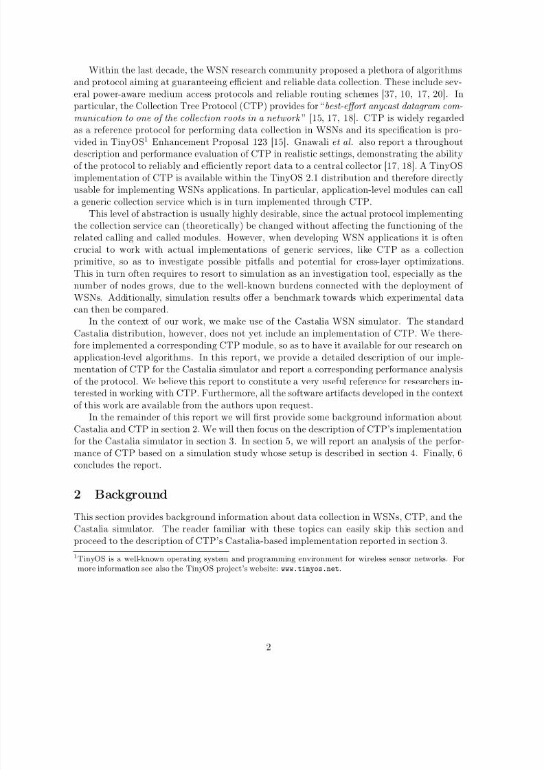
To gather the necessary statistics and compute the 1-hop ETX, the LE adds a 2 byteheader and a variable length footer to outgoing routing beacons. To this end, as shown infigure 1, routing beacons are passed over by the RE to the LE before transmission. Thefine-grained structure of LE’s header and footer will be described in section 3.2.
Upon reception of a beacon, the LE extracts the information from both the header and
4
8/4/2019 CTP Over Castalia
http://slidepdf.com/reader/full/ctp-over-castalia 5/47
Figure 1: Message flow and modules interactions.
footer and includes it in the so-called link estimator table [17]. This table holds a list of identifiers of the neighbors of a node, along with related information, like their 1-hop ETX orthe amount of time elapsed since the ETX of a specific neighbor has been updated. In contrastto the routing table, which is maintained by the RE, the link estimator table is created andupdated by the LE. These tables are however tightly coupled. For instance, the RE can forcethe LE to add an entry to the link estimator table or to block a removal. The latter caseoccurs when one of the neighbors is the sink node. Similarly, the LE can signal the evictionof a specific node from the link estimator table to the RE, which in turn accordingly removesthe entry corresponding to the same node in the routing table. The information availablefrom the link estimator table is used to fill the footer of outgoing beacons, so that nodes canefficiently share neighborhood information. However, the space available in the footer maynot be sufficient to include all the entries of the neighborhood table in one single beacon.Therefore, the entries to send are selected following a round robin procedure over the linkestimator table.
Interfaces. As we will also detail in the following section 3, the three components RE, FE,and LE do not work independently but interact through a set of well-defined interfaces. Forinstance, the RE needs to pull the 1-hop ETX metric from the LE to compute the multi-hopETX. On the other side, the FE must obtain the identifier of the current parent from the REand check the congestion status of the neighbors with the RE. As schematically depicted infigure 1, these interactions are managed by specific interfaces. In the following section 3, wewill explicitly mention these interfaces whenever necessary or appropriate.
5

8/4/2019 CTP Over Castalia
http://slidepdf.com/reader/full/ctp-over-castalia 6/47
2.3 Castalia and OMNeT++
There exist a plethora of different frameworks that provide comfortable simulation environ-ments for WSNs applications. Their survey is beyond the scope of this report and the inter-ested reader is referred to [19, 13]. In the context of our work, we are interested in simulationenvironments that provide for modularity, realistic radio and channel models, and, at the
same time, comfortable programming. To the best of our knowledge, among the currentlyavailable frameworks the Castalia WSNs simulator emerges for its quality and completeness[26, 21, 27, 33]. Castalia provides a generic platform to perform “ first order validation of an algorithm before moving to an implementation on a specific platform ” [2]. It is basedon the well-known OMNet++ simulation environment, which mainly provides for Castalia’smodularity.
OMNeT++ is a discrete event simulation environment that thanks to its excellent modu-larity is particularly suited to support frameworks for specialized research fields. For instance,it supports the Mobility Framework (MF) to simulate mobile networks, or the INET frameworkthat models several internet protocols. OMNeT++ is written in C++, is well documentedand features a graphical environment that eases development and debugging. Additionally, a
wide community of contributors supports OMNeT++ by continuously providing updates andnew frameworks. The comfortable initial training, the modularity, the possibility of program-ming in an object-oriented language (C++), are among the reasons that led us to prefer theOMNeT++ platform, and thus Castalia, over other available network simulators like the well-known ns2 and the related extensions for WSNs (e.g., SensorSim [30]). Nonetheless, in thelast years Castalia has been continuously improved [7, 31] and there is an increasing numberof researchers using Castalia to support their investigations [8, 36, 5, 22, 4].
In the context of this work, we make use of version 1.3 of Castalia, which builds uponversion 3.3 of OMNeT++. In this version, Castalia features advanced channel and radiomodels, a MAC protocol with large number of tunable parameters and a highly flexible modelfor simulating physical processes. In contrast to other frameworks for wireless sensor networks,
Castalia offers exhaustive models for simulating both the radio channel and the physical layerof the radio module. In particular, Castalia provides bundled support for the CC 2420 radiocontroller, which is the transceiver of choice for the TelosB/TmoteSky platform [12, 32]. Thisis particularly relevant to us since the Tmote Sky is our reference hardware platform.
3 Implementation of CTP
Being a simulator originally developed mainly for MAC protocols testing, Castalia offers only abasic hop distance routing layer in its original distribution. Thanks to the excellent modularityinherited from OMNeT++, however, Castalia can be easily extended and adapted to includenew components. Hence, we have implemented a CTP routing module for Castalia that
mimics, as far as possible, TinyOS 2.1 reference implementation of CTP [15, 17]. The hopdistance routing protocol available in the standard Castalia distribution can be transparentlyreplaced by our CTP module.
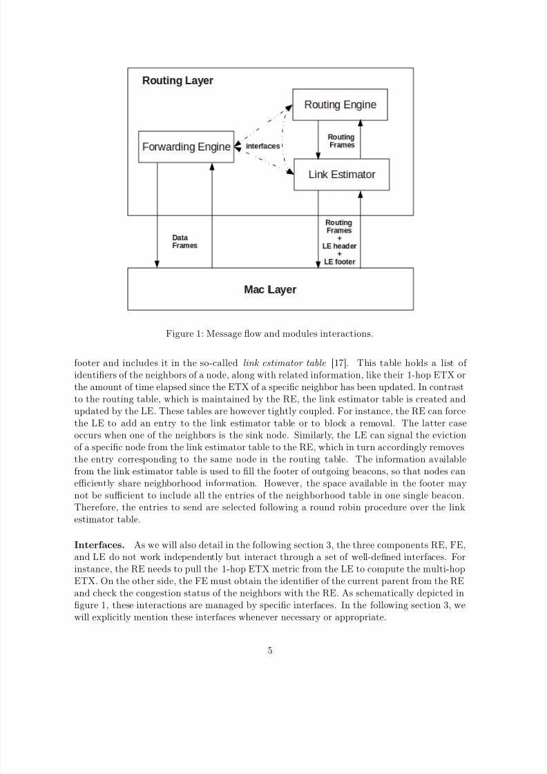
Figure 2 shows the basic architecture of our implementation. The three modules LinkEstimator, Routing Engine, and Forwarding Engine clearly provide the same functionalities of the correspondent components described in section 2.2. The full implementation is included ina compound module, which we dubbed CTPRouting , and that includes also the CTPProtocolmodule. CTPProtocol provides marshaller functionalities by managing incoming and outgoing
6

8/4/2019 CTP Over Castalia
http://slidepdf.com/reader/full/ctp-over-castalia 7/47
messages between the CTPRouting compound module and its internal components. Thus,only the CTPProtocol module is connected to the input and output gates of the CTPRoutingcompound module. The LE, RE, and FE must therefore interact with the CTPProtocolmodule to dispatch their messages to other (internal or external) modules. The dotted lines infigure 2 represent direct method calls.2 Indeed, the internal modules of a compound module
may use a common set of functions. These function may be implemented in only one of themodules and used by the others through the above mentioned direct calls.Figure 2 also shows that our CTPRouting module interacts with the application and
physical layers through the Application and TunableMAC modules, respectively. In particular,our CTPRouting module implements the same connections to both the Application and theTunableMAC modules as Castalia’s default routing module. Embedding our implementationof CTP within the standard distribution of Castalia is thus straightforward, since it cantransparently replace the default routing module. However, since CTP poses some constraintson the underlying MAC layer, a few changes to the TunableMAC module have been necessaryin order to make our CTPRouting module work. We describe these changes in section 3.5.
Figure 2: Architecture of the CTPRouting compound module.
The values of the relevant parameters of our Castalia-based implementation of CTP arelisted in the corresponding ctpRouting.ini configuration file. We would like to point out
that our Castalia-based implementation of CTP has been developed on top of the versions3.3 and 1.3 of OMNeT++ and Castalia, respectively. Although these distribution are by nowout-of-date3, the considerations reported below still hold and the developed software moduleswould need minor adjustments only in order to run on the newer versions of the platforms.
In the remainder of this section we will describe our implementation of the LE, RE, and
2Please refer to the OMNeT++ user manual for a formal definition of module , compound module , direct method call and their usage [29].
3As of August 2010, versions 4.1 and 3 of OMNeT++ and Castalia are available.
7
8/4/2019 CTP Over Castalia
http://slidepdf.com/reader/full/ctp-over-castalia 8/47
FE and then detail about the changes we had to carry out on the TunableMAC module. Wewill particularly focus on the most tricky implementation issues and thus assume the readerhas some familiarity with the topic at hand. Before going into further details, however, wefirst describe the structure of both the routing and data messages handled by CTP. Withineach of the following subsections we organized the content in paragraphs so as to improve the
readability of the text.
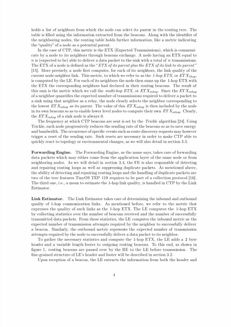
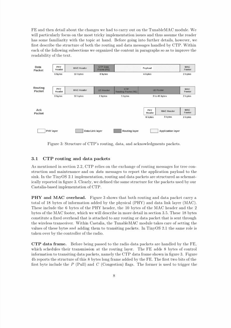
Figure 3: Structure of CTP’s routing, data, and acknowledgments packets.
3.1 CTP routing and data packets
As mentioned in section 2.2, CTP relies on the exchange of routing messages for tree con-
struction and maintenance and on data messages to report the application payload to thesink. In the TinyOS 2.1 implementation, routing and data packets are structured as schemat-ically reported in figure 3. Clearly, we defined the same structure for the packets used by ourCastalia-based implementation of CTP.
PHY and MAC overhead. Figure 3 shows that both routing and data packet carry atotal of 18 bytes of information added by the physical (PHY) and data link layer (MAC).These include the 6 bytes of the PHY header, the 10 bytes of the MAC header and the 2bytes of the MAC footer, which we will describe in more detail in section 3.5. These 18 bytesconstitute a fixed overhead that is attached to any routing or data packet that is sent throughthe wireless transceiver. Within Castalia, the TunableMAC module takes care of setting the
values of these bytes and adding them to transiting packets. In TinyOS 2.1 the same role istaken over by the controller of the radio.
CTP data frame. Before being passed to the radio data packets are handled by the FE,which schedules their transmission at the routing layer. The FE adds 8 bytes of controlinformation to transiting data packets, namely the CTP data frame shown in figure 3. Figure4b reports the structure of this 8 bytes long frame added by the FE. The first two bits of thefirst byte include the P (Pull) and C (Congestion) flags. The former is used to trigger the
8

8/4/2019 CTP Over Castalia
http://slidepdf.com/reader/full/ctp-over-castalia 9/47
Figure 4: Structure of CTP’s routing (a) and data (b) frames, along with the header andfooter added by the LE (c).
sending of beacon frames from neighbors for topology update, while the latter allows a node tosignal that it is congested. As we will detail in section 3.4, if a node receives a routing beaconfrom a neighbor with the C flag set, it will stop sending packets to this neighbor and look foralternatives routes, so as to release the congested node. The last 6 bits of the first byte arereserved for future use (e.g., additional flags). The second byte reports the THL (Time Has
Lived) metric. The THL is a counter that is incremented by one at each packet forwarding andthus indicates the number of hops a packet has effectively traveled before reaching the currentnode. The third and fourth bytes are reserved for the (multi-hop) ETX metric, which weintroduced in section 2, while the fifth and sixth constitute the Origin field, which includes theidentifier of the node that originally sent the packet. The originating node also sets the 1-bytelong SeqNo field, which specifies the sequence number of the packet. Further, the CollectId is an identifier specifying which instance of a collection service is intended to handle thepacket. Indeed, in TinyOS 2.1 CTP can manage multiple application level components. Eachof these components is assigned a unique CollectId identifier, which allows differentiating oneapplication flow from the other [15]. Figure 3 finally shows that data packets carry a payloadof n bytes, whereby the actual length n of the payload clearly depends on the application
logic.
CTP routing frame. As mentioned above, CTP relies on information shared by neighbor-ing nodes through the sending of routing packets in order to build and maintain the routingtree. While data packets are handled by the FE only, routing packets are generated andprocessed by both the RE and LE. As shown in figure 3 routing packets carry, in addition tothe PHY and MAC overhead, a 2 bytes header and a variable length footer which are set by
9

8/4/2019 CTP Over Castalia
http://slidepdf.com/reader/full/ctp-over-castalia 10/47
the LE and will be described in the following section 3.2. The actual CTP routing frame is5 bytes long and its fine-grained structure is reported in figure 4a. As for data frames, thefirst byte of a CTP routing frame includes the P and C flags and 6 unused bits. The secondand third bytes host the Parent field, which specifies the identifier of the parent of the nodesending the beacon. The fourth and fifth byte finally include the (multi-hop) ETX metric.
Please note that while the multi-hop path ETX is stored over 2 bytes, the 1-hop ETX onlyneeds 1 byte.
Acknowledgments. For the sake of completeness figure 3 also shows the structure of ac-knowledgment (Ack) packets, which are used to notify the successful reception of a data packetto the sender of the packet. Since CTP makes use of link-layer acknowledgments, Ack packetsonly include PHY and MAC layer information for a total of 11 bytes.
3.2 Link Estimator module
As discussed in section 2.2 and reported in [17], the Link Estimator is mainly responsible fordetermining the quality of the communication link. In TinyOS 2.1, the LE is implemented by
the LinkEstimatorP.nc component, located in in the folder /tos/lib/net/4bitle.4
LE header and footer. Figure 4c shows the structure of the header and footer added bythe LE to routing packets before they are passed over to the radio for transmission. The firstbyte of the header, namely the NE (Number of Entries) field, encodes the length of the footer.This value is actually encoded in 4 bits only while the remaining 4 are reserved for futureuse. The second byte includes the SeqNo field, which represents a sequence number that isincremented by one at every beacon transmission. By counting the number of beacons actuallyreceived from each neighbor and comparing this number with the corresponding SeqNo, theLE can estimate the number of missing beacons over the total number of beacons sent by aspecific neighbor.
While the header has a fixed length of 2 bytes, the footer has a variable length which isupper bounded by the residual space available on the beacon. The footer carries a variablenumber of <etx,address> couples, each of 3 bytes in length, including the 1-hop ETX (1 byte)and the address (2 bytes) of neighboring nodes. Please recall that the 1-hop ETX requiresonly 1 byte to be stored while the multi-hop ETX requires 2 bytes. As mentioned in section2.2, the entries included in LE’s footer are selected following a round robin procedure over thelink estimator table. Since the maximal length of the footer is of 45 bytes, the total size of arouting packet from 25 to 70 bytes, as also shown in figure 3.
Although the use of the footer is foreseen in CTP’s original design [17, 18], the TinyOS2.1 implementation of CTP does not make use of it and so neither does our Castalia-basedimplementation5.
Computation of the 1-hop ETX. For each neighbor, the LE determines the 1-hop ETXconsidering the quality of both the ingoing and outgoing links. The quality of the outgoing linkis computed as follows. Let nu be the number of unicast packets sent by the node (including
4For the sake of simplicity, we assume that for all the TinyOS paths listed in this report the root / refers tothe root of the TinyOS 2.1 distribution (e.g., tinyos-2.x/ ).
5Another implementation of the LE, described in revision 1.8 of TEP 123 and available in /tos/lib/net/le
does use the footer.
10
8/4/2019 CTP Over Castalia
http://slidepdf.com/reader/full/ctp-over-castalia 11/47
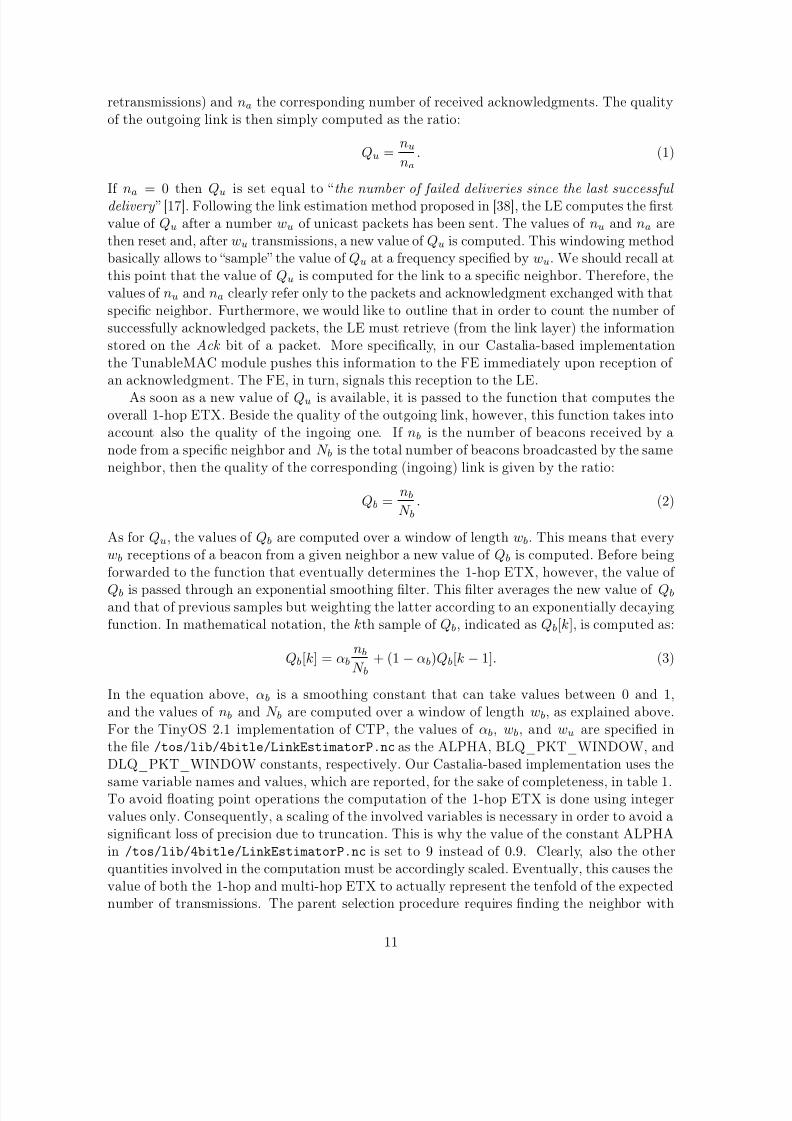
retransmissions) and na the corresponding number of received acknowledgments. The qualityof the outgoing link is then simply computed as the ratio:
Qu =nu
na. (1)
If na = 0 then
Qu is set equal to “the number of failed deliveries since the last successful delivery ” [17]. Following the link estimation method proposed in [38], the LE computes the first
value of Qu after a number wu of unicast packets has been sent. The values of nu and na arethen reset and, after wu transmissions, a new value of Qu is computed. This windowing methodbasically allows to “sample” the value of Qu at a frequency specified by wu. We should recall atthis point that the value of Qu is computed for the link to a specific neighbor. Therefore, thevalues of nu and na clearly refer only to the packets and acknowledgment exchanged with thatspecific neighbor. Furthermore, we would like to outline that in order to count the number of successfully acknowledged packets, the LE must retrieve (from the link layer) the informationstored on the Ack bit of a packet. More specifically, in our Castalia-based implementationthe TunableMAC module pushes this information to the FE immediately upon reception of an acknowledgment. The FE, in turn, signals this reception to the LE.
As soon as a new value of Qu is available, it is passed to the function that computes theoverall 1-hop ETX. Beside the quality of the outgoing link, however, this function takes intoaccount also the quality of the ingoing one. If nb is the number of beacons received by anode from a specific neighbor and N b is the total number of beacons broadcasted by the sameneighbor, then the quality of the corresponding (ingoing) link is given by the ratio:
Qb =nb
N b. (2)
As for Qu, the values of Qb are computed over a window of length wb. This means that everywb receptions of a beacon from a given neighbor a new value of Qb is computed. Before beingforwarded to the function that eventually determines the 1-hop ETX, however, the value of
Qb is passed through an exponential smoothing filter. This filter averages the new value of Qb
and that of previous samples but weighting the latter according to an exponentially decayingfunction. In mathematical notation, the kth sample of Qb, indicated as Qb[k], is computed as:
Qb[k] = αbnb
N b+ (1 − αb)Qb[k − 1]. (3)
In the equation above, αb is a smoothing constant that can take values between 0 and 1,and the values of nb and N b are computed over a window of length wb, as explained above.For the TinyOS 2.1 implementation of CTP, the values of αb, wb, and wu are specified inthe file /tos/lib/4bitle/LinkEstimatorP.nc as the ALPHA, BLQ_PKT_WINDOW, andDLQ_PKT_WINDOW constants, respectively. Our Castalia-based implementation uses the
same variable names and values, which are reported, for the sake of completeness, in table 1.To avoid floating point operations the computation of the 1-hop ETX is done using integervalues only. Consequently, a scaling of the involved variables is necessary in order to avoid asignificant loss of precision due to truncation. This is why the value of the constant ALPHAin /tos/lib/4bitle/LinkEstimatorP.nc is set to 9 instead of 0.9. Clearly, also the otherquantities involved in the computation must be accordingly scaled. Eventually, this causes thevalue of both the 1-hop and multi-hop ETX to actually represent the tenfold of the expectednumber of transmissions. The parent selection procedure requires finding the neighbor with
11

8/4/2019 CTP Over Castalia
http://slidepdf.com/reader/full/ctp-over-castalia 12/47
Link Estimator
Parameter Value Unit
αETX 0.9 -
αb 0.9 -
wb 3 packets
wu 5 packetsSize of link estimator table 10 entries
Header length 2 bytes
Footer length < 45 bytes
Table 1: Values of relevant parameters of the Link Estimator module.
the lowest ETX, irrespectively of the absolute values, and it is thus not affected by the abovementioned scaling. For further details on this issue we refer the reader to the well-documented/tos/lib/4bitle/LinkEstimatorP.ncfile.
Each time a new value of Qu or Qb for a specific neighbor is available, the 1-hop ETXmetric relative to the same neighbor is accordingly updated. As for Qb, the update procedureuses an exponential smoothing filter. Let Q be the new value of either Qu or Qb and ETX old1hop
the previously computed value of the 1-hop ETX. The updated value of the ETX 1hop is thencomputed as follows:
ETX 1hop = αETXQ + (1 − αETX)ETX old1hop. (4)
In the standard implementation of the LE the smoothing constant αETX is set to 0.9. As men-tioned above, however, the value of αETX used within the /tos/lib/4bitle/LinkEstimatorP.ncfile is the tenfold of the “theoretical” one, thus 9 instead of 0.9.
After each update, the value of the 1-hop ETX is stored in the link estimator table along
with the corresponding neighbor identifier.
Insertion/eviction procedure of the link estimator table. When a beacon from aneighbor that is not (yet) included in the link estimator table is received, the LE first checkswhether there is a free slot in the table to allocate the newly discovered neighbor. If the link es-timator table is not filled, the LE simply inserts the new entry in one of the free available slots.In the TinyOS 2.1 implementation of CTP the maximal number of neighbors that can be in-cluded in the link estimator table is 10. A different value can be used by accordingly setting thevariable NEIGHBOR_TABLE_SIZE in the file /tos/lib/net/4bitle/LinkEstimator.h.
If the link estimator table is filled but it includes at least one entry that is not valid , thenthe LE replaces the first found non valid entry with the new neighbor. An entry of the link
estimator table becomes valid as soon as it is included in the table and turns not valid if it isnot updated within a fixed timeout. For instance, the entry corresponding to a neighbor that(even if only temporarily) loses connectivity may become not valid. Beside the valid flag theLE also sets, for each entry of the link estimator table, a mature and pinned flag. The formeris set to 1 when the first estimation of the 1-hop ETX of a new entry of the neighborhoodtable becomes available. This happens after at least one value of Qb or Qu can be computed.Instead, the pinned flag, or pin bit, is set to 1 if the multi-hop ETX of a node is 0, and thusthe node is the root of a routing tree, or if a neighbor is the currently selected parent. The
12

8/4/2019 CTP Over Castalia
http://slidepdf.com/reader/full/ctp-over-castalia 13/47
pin bit is set at the routing layer and its value is propagated to the LE and its link estimatortable.
If the link estimator table is filled and all of its entries are valid, then the LE verifies if there exist (valid, mature, and non pinned) entries whose 1-hop ETX is higher than a giventhreshold. This threshold is set to a high value6 and it thus allows individuating unreliable
communication partners. Among these nodes, the one with the worst (i.e., highest) 1-hopETX is evicted from the table and the new neighbor is inserted in place of it. The value of the1-hop ETX of the new neighbor is irrelevant at this point since it is not yet available. Indeed,the computation of the 1-hop ETX can only start after a node has been inserted in the linkestimator table and the values of Qu and Qb start being computed.
If none of the entries of the link estimator table is eligible for eviction as described above,then the LE determines whether to insert the new neighbor anyway or discard it. The LEforces an insertion of the new neighbor in two cases. First, if it is the root of a routing tree andthus the multi-hop ETX declared in the received beacon is set to 0. Second, if the multi-hopETX of the new neighbor is lower (i.e., better) than at least one of the (valid, mature, and nonpinned) entries of the routing table. This latter step clearly requires contacting the RoutingEngine in order to retrieve the information related to the multi-hop ETX. To this end, the
LE requests the RE to return the value of the so-called compare bit. If the compare bit is setto 1, then the new neighbor must be inserted, if it set to 0 the new neighbor is discarded.
If the LE determines the new neighbor should be inserted, then it randomly chooses onethe existing (non pinned) entries and replaced it with the new neighbor. The flow chartcorresponding to the above described eviction/insertion procedure is reported in figure 5.
The white bit. In the original design of CTP [17] not all beacons received from neighborsthat are not included in the link estimator table are considered for insertion. In particular,upon reception of such a beacon the LE first checks if the corresponding probability of de-coding error (averaged over all symbols) is higher than a given quality threshold. Better said,the LE requires the physical layer to return the value of 1 bit of information, the so-called
white bit. If the bit is set to 1, then the packet is considered for insertion otherwise it isimmediately discarded. The white bit thus “provides a fast and inexpensive way to avoid borderline or marginal links ” [17]. In the TinyOS 2.1 implementation of the LE, however,this information is not considered during the neighbor eviction process and so neither doesour Castalia-based implementation. We refer to the CompareBit.shouldInsert function in/tos/lib/net/ctp/RoutingEngine.nc for further details on this issue.
4-bits Link Estimator. As the above description makes clear the LE has two main tasks:populating the link estimator table with the “best possible” neighbors and computing their1-hop ETX. To comply with both tasks, the LE retrieves information from TunableMAC, FE,and RE modules. In particular, the LE needs to retrieve the values of the ack, white, pin, and
compare bits, which have been described above. Since it makes use of these 4 state bits, theLE is also called 4-bit LE .
Differences between actual implementation and original design. The actual defaultimplementation of the Link Estimator in TinyOS 2.1 can be found in /tos/lib/net/4bitle
655 in the TinyOS 2.1 implementation of CTP. See also the EVICT_EETX_THRESHOLD constant in/tos/lib/net/4bitle/LinkEstimatorP.nc).
13

8/4/2019 CTP Over Castalia
http://slidepdf.com/reader/full/ctp-over-castalia 14/47
Figure 5: Insertion policy for LE’s link estimator table.
14
8/4/2019 CTP Over Castalia
http://slidepdf.com/reader/full/ctp-over-castalia 15/47
and is described in revision 1.15 of TEP 123 [15]. As noted above, this implementation (andthus also our Castalia-based one) differs from CTP’s original design in two points. First, thewhite bit is not considered during the LE’s table insertion/eviction procedure. Second, theentries included in the footer of routing beacons are not used for populating the link estimatorand routing tables.
3.3 Routing Engine module
The main tasks of the Routing Engine consist in sending beacons, filling the routing table,keeping it up to date, and selecting a parent in the routing tree towards which data framesmust be routed. We recall at this point that CTP’s routing frames are 5 bytes long, as shownin figure 4a. To derive the total size of a beacon, however, the overhead (headers and footers)added by the LE and the physical and link layers must also be considered, as we discussed insection 3.1.
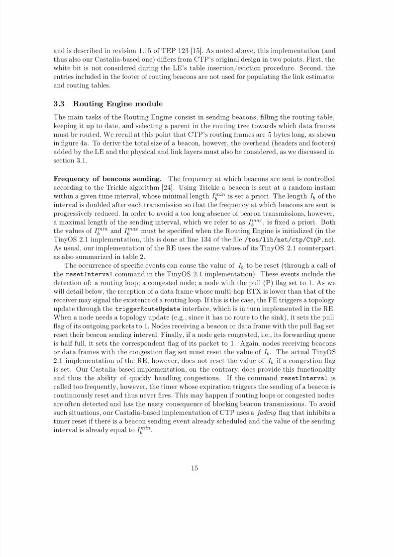
Frequency of beacons sending. The frequency at which beacons are sent is controlledaccording to the Trickle algorithm [24]. Using Trickle a beacon is sent at a random instant
within a given time interval, whose minimal length I minb is set a priori. The length I b of theinterval is doubled after each transmission so that the frequency at which beacons are sent isprogressively reduced. In order to avoid a too long absence of beacon transmissions, however,a maximal length of the sending interval, which we refer to as I max
b , is fixed a priori. Boththe values of I min
b and I maxb must be specified when the Routing Engine is initialized (in the
TinyOS 2.1 implementation, this is done at line 134 of the file /tos/lib/net/ctp/CtpP.nc).As usual, our implementation of the RE uses the same values of its TinyOS 2.1 counterpart,as also summarized in table 2.
The occurrence of specific events can cause the value of I b to be reset (through a call of the resetInterval command in the TinyOS 2.1 implementation). These events include thedetection of: a routing loop; a congested node; a node with the pull (P) flag set to 1. As we
will detail below, the reception of a data frame whose multi-hop ETX is lower than that of thereceiver may signal the existence of a routing loop. If this is the case, the FE triggers a topologyupdate through the triggerRouteUpdate interface, which is in turn implemented in the RE.When a node needs a topology update (e.g., since it has no route to the sink), it sets the pullflag of its outgoing packets to 1. Nodes receiving a beacon or data frame with the pull flag setreset their beacon sending interval. Finally, if a node gets congested, i.e., its forwarding queueis half full, it sets the correspondent flag of its packet to 1. Again, nodes receiving beaconsor data frames with the congestion flag set must reset the value of I b. The actual TinyOS2.1 implementation of the RE, however, does not reset the value of I b if a congestion flagis set. Our Castalia-based implementation, on the contrary, does provide this functionalityand thus the ability of quickly handling congestions. If the command resetInterval is
called too frequently, however, the timer whose expiration triggers the sending of a beacon iscontinuously reset and thus never fires. This may happen if routing loops or congested nodesare often detected and has the nasty consequence of blocking beacon transmissions. To avoidsuch situations, our Castalia-based implementation of CTP uses a fading flag that inhibits atimer reset if there is a beacon sending event already scheduled and the value of the sendinginterval is already equal to I min
b .
15
8/4/2019 CTP Over Castalia
http://slidepdf.com/reader/full/ctp-over-castalia 16/47
Routing Engine
Parameter Value Unit
Minimal length of the beacon window 63 ms
Maximal length of the beacon window 250 s
Size of the routing table 10 entries
Parent switch threshold 15 -Parent refresh period 8 s
Beacon Packet size 5 bytes
Table 2: Values of relevant parameters of the Routing Engine module.
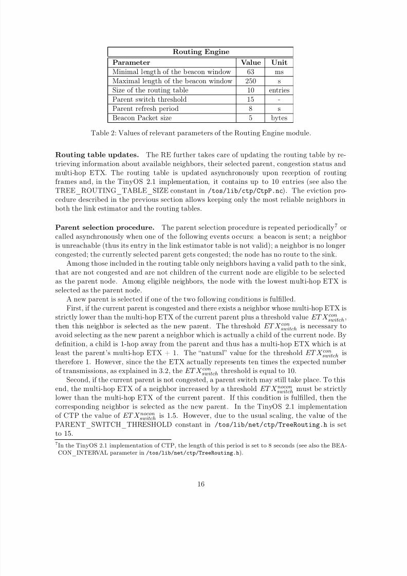
Routing table updates. The RE further takes care of updating the routing table by re-trieving information about available neighbors, their selected parent, congestion status andmulti-hop ETX. The routing table is updated asynchronously upon reception of routingframes and, in the TinyOS 2.1 implementation, it contains up to 10 entries (see also theTREE_ROUTING_TABLE_SIZE constant in /tos/lib/ctp/CtpP.nc). The eviction pro-
cedure described in the previous section allows keeping only the most reliable neighbors inboth the link estimator and the routing tables.
Parent selection procedure. The parent selection procedure is repeated periodically7 orcalled asynchronously when one of the following events occurs: a beacon is sent; a neighboris unreachable (thus its entry in the link estimator table is not valid); a neighbor is no longercongested; the currently selected parent gets congested; the node has no route to the sink.
Among those included in the routing table only neighbors having a valid path to the sink,that are not congested and are not children of the current node are eligible to be selectedas the parent node. Among eligible neighbors, the node with the lowest multi-hop ETX isselected as the parent node.
A new parent is selected if one of the two following conditions is fulfilled.First, if the current parent is congested and there exists a neighbor whose multi-hop ETX isstrictly lower than the multi-hop ETX of the current parent plus a threshold value ETX conswitch,then this neighbor is selected as the new parent. The threshold ETX conswitch is necessary toavoid selecting as the new parent a neighbor which is actually a child of the current node. Bydefinition, a child is 1-hop away from the parent and thus has a multi-hop ETX which is atleast the parent’s multi-hop ETX + 1. The “natural” value for the threshold ETX conswitch istherefore 1. However, since the the ETX actually represents ten times the expected numberof transmissions, as explained in 3.2, the ETX conswitch threshold is equal to 10.
Second, if the current parent is not congested, a parent switch may still take place. To thisend, the multi-hop ETX of a neighbor increased by a threshold ETX noconswitch must be strictlylower than the multi-hop ETX of the current parent. If this condition is fulfilled, then the
corresponding neighbor is selected as the new parent. In the TinyOS 2.1 implementationof CTP the value of ETX noconswitch is 1.5. However, due to the usual scaling, the value of thePARENT_SWITCH_THRESHOLD constant in /tos/lib/net/ctp/TreeRouting.h is setto 15.7In the TinyOS 2.1 implementation of CTP, the length of this period is set to 8 seconds (see also the BEA-
CON_INTERVAL parameter in /tos/lib/net/ctp/TreeRouting.h).
16

8/4/2019 CTP Over Castalia
http://slidepdf.com/reader/full/ctp-over-castalia 17/47
3.4 Forwarding Engine module
The main task of the Forwarding Engine consist in forwarding data packets received fromneighboring nodes as well as sending packets generated by the application module of thenode. Additionally, the FE is responsible for recognizing the occurrence of duplicate packetsand routing loops. Last but not least, the FE also works as a snooper and listens to data
packets addressed to other nodes in order to timely detect a topology update request or acongestion status.
Packet queue and retransmissions. The FE stores the data packets to send in a FIFOqueue whose length is set to 12 in the TinyOS 2.1 implementation (see the FORWARD_COUNTconstant in /tos/lib/net/ctp/CtpP.nc). To forward a packet, the FE first retrieves the iden-tifier of the current parent from the RE. If the parent is not congested the FE calls the send procedure thereby appending to the packet the 8 bytes long CTP data frame shown in figure4b. Otherwise, if the parent is congested, it waits until the congestion status of the parentchanges or a new parent is selected. After sending a packet the FE awaits for a correspondingacknowledgment before removing it from the head of the queue. If the acknowledgment is not
received within a given time interval, the FE will try and retransmit it until a pre-specifiedmaximum of retransmission attempts have been performed. After the maximal number of retransmission attempts have been reached, the packet is discarded. In the TinyOS 2.1 imple-mentation the maximal number of retransmissions is set to 30 (see also the MAX_RETRIESparameter in /tos/lib/net/ctp/CtpForwardingEngine.h), and so it is in our Castalia-basedversion.
Congestion flag. If a node is chosen as parent from several neighbors, or if it must performmany retransmissions attempts, the queue of its FE may quickly fill up with unsent packets.Since this may eventually cause the node to drop further incoming packets the FE notifiesthis congestion status by setting the C flag of outgoing data frames to 1. In particular, the
FE declares the node as congested as soon as half of its packet queue is full. Additionally,the FE also notifies the congestion status to the RE, which takes care of setting also the Cflag of routing frames to 1. This simple mechanism allows the protocol to (re-)distribute thecommunication load over of the network since a congested node is unlikely to be selected asparent (see also section 3.3). Optionally, the FE can call the command setClientCongested
to force the RE to reset the beacon sending interval as soon as a congestion state is detected.Despite increasing the number of transmitted beacons, this option allows nodes to timelynotify their congestion status, thus improving the reactiveness of the network. Our simulationstudy showed that by activating this option we often can significantly decrease the number of packets dropped due to congested nodes. For this reason the setClientCongested option isalways enabled in our Castalia-based implementation of CTP.
Duplicate packets. In order to detect duplicate packets, the FE evaluates the tuple <Origin,CollectId, SeqNo, THL> for each incoming data packet. As described in section 2.2, the Ori-gin parameter specifies the identifier of the node which originally sent the packet; SeqNo isthe sequence number of the current frame; and the THL is the hop count of the packet. TheCollectId field identifies a specific instance of CTP. If only a single instance of CTP is active,the CollectId field is not relevant and can be ignored during duplicate detection. Thus, thetuple <Origin, CollectId, SeqNo, THL> represents a unique packet instance. By comparing
17

8/4/2019 CTP Over Castalia
http://slidepdf.com/reader/full/ctp-over-castalia 18/47
Forwarding Engine
Parameter Value Unit
Forwarding queue size 12 packets
LRU Cache size 4 packets
Max tx retries 30 -
TX_OK backoff 15.6 - 30.3 msTX_NOACK backoff 15.6 - 30.3 ms
CONGESTION backoff 15.6 - 30.3 ms
LOOP backoff 62.5 - 124 ms
Header size 8 bytes
Table 3: Values of relevant parameters of the Forwarding Engine module.
the value of the tuple of an incoming packet with that of the packets stored in the forwardingqueue, the FE can detect duplicates. The FE also maintains an additional cache to store thelast 4 successfully transmitted packets. Using this cache, duplicates detection can be per-
formed also over recently transmitted packets that are no more available in the forwardingqueue.
Routing loops. The FE also features a mechanism to detect the occurrence of routingloops. To this end, the FE compares the (multi-hop) ETX of each incoming packet with the(multi-hop) ETX of the current node. In particular, since the ETX is an additive metricover the whole routing path and the current node is selected as a parent by the sender of thepacket, then the ETX of the sender must be strictly higher than the ETX of the receiver (i.e.,the current node). If this is not the case, the FE executes a loop management procedure thatfirst of all starts the so-called LOOP backoff timer, resets the beacon sending interval and setsthe pull flag to 1 in order to force a topology update. The FE does not forward any packets
until the expiration of the LOOP timer so that the radio is used to propagate routing beaconsand repair the routing loop. The LOOP timer is thus usually significantly higher than thebeacon sending interval. It is important to note that if a data packet is forwarded during theexecution of the loop management procedure, then the packet continues being forwarded overthe loop until a new path to the sink is established. Since the THL field is increase at eachretransmission, the packet cannot be erroneously recognized as a duplicate.
FE’s snooping mechanism. A further interesting feature of the FE consists in its ability tooverhear unicast data packets addressed to other nodes. This behavior, referred to as snooping ,allows CTP to quickly react to congestion notifications or topology update requests carriedby the C and P flags of the snooped data frame. In TinyOS 2.1, the Snoop interface usedby the FE is implemented within the CC2420ActiveMessageP component, which is locatedin the /tos/chips/cc2420/ folder. In our Castalia-based implementation, the TunableMACmodule notifies the FE when such snooped packets are available. To this end, we created anew MAC_2_NETWORK_SNOOP_MSGmessage within the TunableMAC module, as we detail in thefollowing section 3.5.
Backoff timers. Last but not least, the FE also manages the backoff timers, i.e., thetimers regulating collision avoidance mechanisms. In particular, the FE sets the TX_OK,
18

8/4/2019 CTP Over Castalia
http://slidepdf.com/reader/full/ctp-over-castalia 19/47
TX_NOACK, CONGESTION, and LOOP backoff timers. The first timer is started aftereach successful packet transmission to balance channel reservation between nodes. The sec-ond has the same function but is activated if the intended receiver of a packet fails to returnthe corresponding acknowledgment. The CONGESTION backoff timer is started when a con-gestion status of the selected parent is detected. When this timer expires, the status of the
parent is evaluated again. Finally, the LOOP timer starts when a loop is detected, as describedabove. Table 3 lists the value of these timers used in both TinyOS 2.1 and our Castalia-basedimplementation of CTP.
3.5 TunableMAC module
TunableMAC is the name of the module that implements MAC functionalities in Castalia.Unfortunately, TunableMAC does not implement all the features that CTP requires to beavailable at the MAC layer and we thus accordingly modified it and added the requiredfeatures.
RE and FE’s packet queues. For instance, in the TinyOS 2.1 implementation of CTP
the RE and the FE both make use of the AMSend TinyOS interface, which offers primitivesfor sending radio packets. In particular, the RE and the FE use two different instances of this interface. Each of these instances holds its own packet queue (with a maximum lengthof one packet each) and the radio component alternatively selects packets from either queues.Instead, the TunableMAC component relies on a single message queue with a freely config-urable maximum length.8 To reproduce in Castalia the same behavior of the TinyOS AMSend
interface we thus added a second message queue in TunableMAC and configured the lengthof both queues to be of 1 packet. Messages coming from the RE or FE are then appropriatelyadded to the corresponding queue. Routing and data frames can be easily distinguished sincethe former are broadcast messages while the latter unicast packets.
FE’s snooping mechanism. As mentioned in section 3.4, the FE implements a snoopingmechanism to timely detect congestion notifications and topology update requests. Since theTunableMAC module is actually designed to discard unicast packets that are not addressedto the current node, a little modification has been necessary to enable FE’s snooping mecha-nism. In particular, we have disabled the packet deletion procedure and implemented a newmechanism that inserts a snooped packet in a MAC_2_NETWORK_SNOOP_MSG message, which isin turn passed to the CTPRouting compound module and finally to the FE module.
Link-layer acknowledgments. An additional feature we needed to add to the TunableMACmodule concerns data link-layer acknowledgments. In particular, CTP requires the receiver of a unicast packet to explicitly acknowledge a successful reception (at the data link-layer) to the
sender of the packet. However, TunableMAC does not provide for data link-layer acknowledge-ments. In order to enhance TunableMAC with this additional feature we first investigatedhow data link-layer acknowledgments are handled by the Chipcon CC 2420, the radio chipembedded on the Telosb/Tmote Sky platform. In particular, upon receiving a unicast packet
8The length of the queue can be set in the omnetpp.ini configuration file. Please refer to the OMNet++ usermanual [29] for further information.
19
8/4/2019 CTP Over Castalia
http://slidepdf.com/reader/full/ctp-over-castalia 20/47
at the MAC level, the CC 2420 controller automatically generates an acknowledgment mes-sage and sends it to the sender of the packet. To this end, the corresponding option must beenabled on the radio chip [11]. On the other side, the sender keeps the packet in its queue (atthe MAC level) and awaits for an acknowledgment. Upon reception of the acknowledgmentthe sender sets the isAck flag on the packet to 1 and triggers the sendDone event that is then
handled at the routing layer. The packet is passed as a parameter along with the sendDoneevent and then removed from the queue so that the next sending operation can be executed.The isAck flag signals the successful reception of the packet to the routing layer of the sender.For further details about this split-phase mechanism, typical of the TinyOS operating system,as well as for more information about the handling of acknowledgments within the CC 2420please refer to [25] and [28, Sect. 5], respectively.
To emulate the behavior of the CC 2420 within the TunableMAC module, we first made itimmediately send an acknowledgment message back to the transmitter as soon as an unicastpacket is received (at the MAC level). Additionally, we defined a new OMNet++ message9,called MAC_2_NETWORK_SEND_DONE, which is sent by the TunableMAC to the CT-PRouting module upon reception of an acknowledgment.
Backoff timers. Regarding (MAC level) backoff timers, we would like to point out that theTinyOS 2.1 distribution the backoff timers of the CC2420 are managed by the component/tos/chips/cc2420/csma/CC2420CsmaP.nc. In particular, the values of the initial and con-gestion backoff timers are set by calling the interfaces initialBackoff and congestionBackoff
of the BMAC protocol. The former timer determines the delay of the first transmission at-tempt while the second is used in the case a busy channel is detected by the radio while sensingthe carrier. Both values are chosen uniformly at random within a pre-specified time intervals,as detailed in table 4. TinyOS 2.1’s /tos/chips/cc2420/CC2420.h file reports the values of these intervals expressed as number of ticks of a 32kHz clock while table 4 reports these samevalues in milliseconds.
The last parameter specified in table 4 is the acknowledgment timeout. This timeout sets
the maximal time interval a sender waits for a packet to be acknowledged. If this timeoutexpires before an acknowledgment has been received, then the packet is passed back to therouting layer along with a message signalling the missing acknowledgment. Clearly, lower-ing the acknowledgment timeout may increase the throughput of the radio but at the sametime cause unnecessary packet retransmissions. Within TinyOS 2.1 the acknowledgment time-out (CC2420_ACK_WAIT_DELAY) is set in the /tos/cc2420/cc2420.h file and expressed as thenumber of ticks of a 32kHz clock.
Packet overhead. Last but not least, we would like to quantify the overhead in terms of bytes that are attached at the MAC layer to both routing and data frames in order to makeCTP work. To this end, we focus on the structure of the packets handled by the CC2420radio chip, which is used on several WSN prototyping platforms, like the Tmote Sky. WithinTinyOS 2.1, the structure of the MAC overhead is defined in the cc2420_header_t struct inthe /tos/chips/cc2420/CC2420.h file, also reported in figure 6. This figure shows that the
9Please refer to the OMNet++ manual for messages definition and handling [29].
20

8/4/2019 CTP Over Castalia
http://slidepdf.com/reader/full/ctp-over-castalia 21/47
TunableMAC
Parameter Value Unit
Initial Backoff range 0.3 - 10 ms
Congestion Backoff range 0.3 - 2.4 ms
PHY overhead 6 bytes
MAC overhead 12 bytesAck Packet size 11 bytes
Ack timeout 7.8 ms
Table 4: Values of relevant parameters of the TunableMAC module.
1 t y p e d e f n x _ s t ru c t c c 24 2 0_ h ea d er _ t {2 n x l e_ u i n t8 _ t l e n g t h ;3 n x le _ ui n t1 6 _t f c f ;4 nxle_uint 8_t dsn ;5 nxle_uint 16_t dest pan ;6 n x l e_ u i n t1 6 _ t d e s t ;7 n x l e_ u i n t1 6 _ t s r c ;
8 nxle_uint 8_t t ype ;9 } cc2420_header_t ;
Figure 6: The cc2420_header_t file.
MAC header contains 7 fields for a total of of 11 bytes. The first field (1 byte) specifies thetotal length of the packet. The fcf and dsn fields occupy 3 bytes and define the values of the Frame Control Field (FCF) and of the Data Sequence Number (DSN). Further, the threefield destpan, dest and src contains the addresses of the sender and intended receiver(s) of the packet. Finally, the field type represents the payload of the MAC layer and indicates theAM (Active Message) identifier of a TinyOS packet [23, Sect. 6].
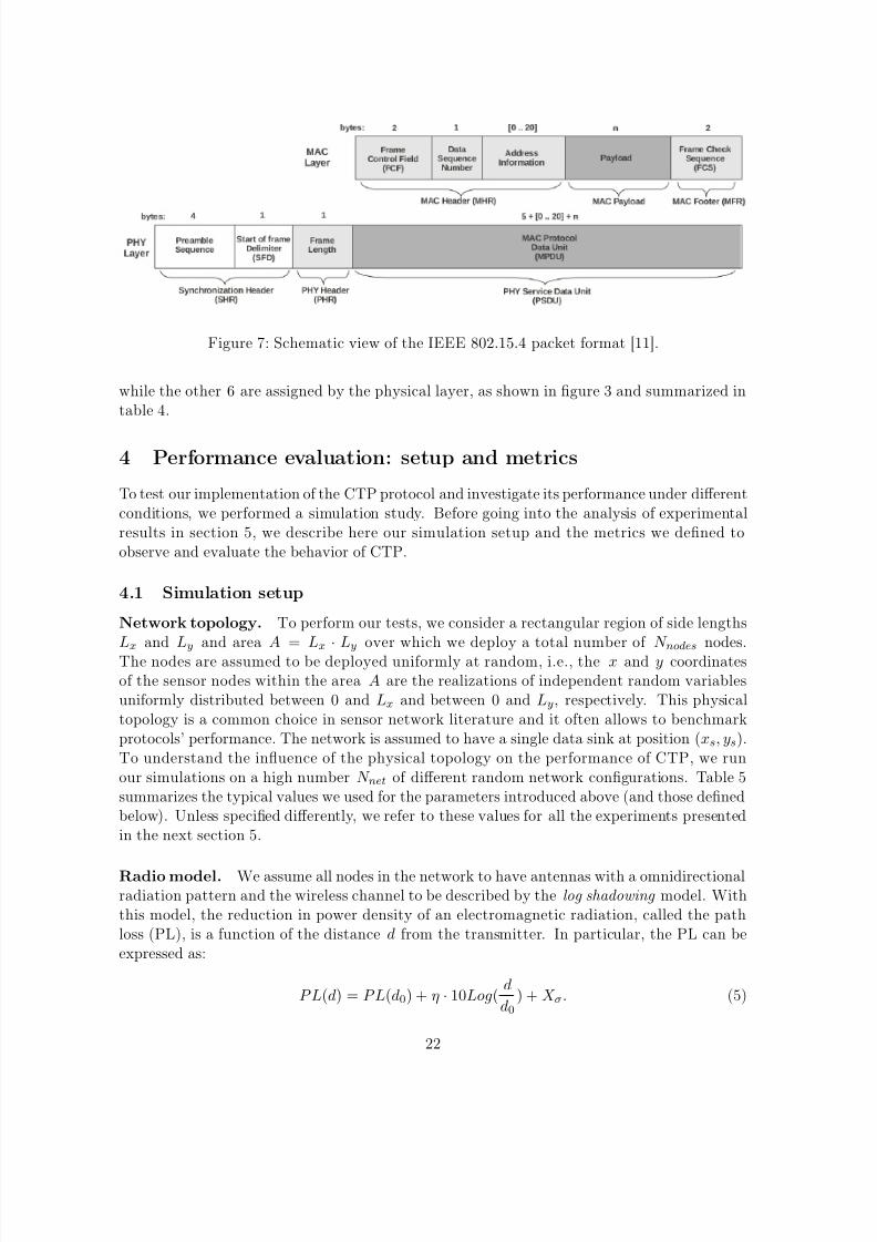
For the sake of completeness, figure 7 reports the generic packet format of a IEEE 802.15.4frame, which is the standard used by the CC2420. This figure shows the control fields addedat both the physical (PHY) and data link (MAC) layers. In particular, the PHY layer adds 3pieces of information for a total of 6 bytes: 4 for the preamble sequence, 1 for frame delimiter,and 1 for the frame length. The MAC layer, in turn, adds further 5 fields, two of which, theaddress information and the payload, of variable length. Comparing figures 6 and 7 we cansee that there are several differences. First of all, the length field is assigned to the PHY layerin figure 6 but appears in the MAC overhead defined by the cc2420_header_t struct. Second,the frame check sequence (FCS) field, which is assigned to the MAC layer in figure 7 does notappear in the cc2420_header_t struct. To be coherent with the IEEE 802.15.4 standard wethus removed the 1 byte of the length field from the computation of the MAC overhead and
added the 2 bytes of the FCS field. We therefore consider a MAC overhead of 12 bytes, 10 forthe header and 2 for the footer, as depicted in figure 3. Also according to figure 3 (and figure7), we consider a PHY overhead of 6 bytes.
The length of packets used for acknowledging the reception of a data message must beconsidered separately. Indeed, acknowledgments are generated within the CC2420 controllerand the corresponding packet format is described in [11, p.22]. According to this format, anacknowledgment packet has a total size of 11 bytes, 5 of which represent MAC layer overhead,
21
8/4/2019 CTP Over Castalia
http://slidepdf.com/reader/full/ctp-over-castalia 22/47
Figure 7: Schematic view of the IEEE 802.15.4 packet format [11].
while the other 6 are assigned by the physical layer, as shown in figure 3 and summarized intable 4.
4 Performance evaluation: setup and metrics
To test our implementation of the CTP protocol and investigate its performance under differentconditions, we performed a simulation study. Before going into the analysis of experimentalresults in section 5, we describe here our simulation setup and the metrics we defined toobserve and evaluate the behavior of CTP.
4.1 Simulation setup
Network topology. To perform our tests, we consider a rectangular region of side lengthsLx and Ly and area A = Lx · Ly over which we deploy a total number of N nodes nodes.The nodes are assumed to be deployed uniformly at random, i.e., the x and y coordinatesof the sensor nodes within the area A are the realizations of independent random variablesuniformly distributed between 0 and Lx and between 0 and Ly, respectively. This physicaltopology is a common choice in sensor network literature and it often allows to benchmarkprotocols’ performance. The network is assumed to have a single data sink at position (xs, ys).To understand the influence of the physical topology on the performance of CTP, we runour simulations on a high number N net of different random network configurations. Table 5summarizes the typical values we used for the parameters introduced above (and those definedbelow). Unless specified differently, we refer to these values for all the experiments presentedin the next section 5.
Radio model. We assume all nodes in the network to have antennas with a omnidirectionalradiation pattern and the wireless channel to be described by the log shadowing model. Withthis model, the reduction in power density of an electromagnetic radiation, called the pathloss (PL), is a function of the distance d from the transmitter. In particular, the PL can beexpressed as:
PL(d) = PL(d0) + η · 10Log(d
d0) + X σ. (5)
22

8/4/2019 CTP Over Castalia
http://slidepdf.com/reader/full/ctp-over-castalia 23/47
Parameter Value Unit
Topology
Lx 250 metersLy 250 metersN nodes 100 -
(xs, y
s) (0,
0) metersRadio model
d0 1 metersPL(d0) 54.2247 dBη 2.4 -X σ 0 -RTX 50 meters
Data Traffic
T s(time) 5 secondsI p [0.5, 1] with step 0.05 -|I p| 11 -
Physical Process
N sources 1 -K 1 -a 2 -V 1(0) 10 -si(0) = (xi(0), yi(0)) (125, 125) meters
General
N net 50 -N rounds 50 -
Table 5: Relevant parameters of our experimental setup and their correspondent values.
In equation 5 PL(d0) represents the (known) path loss at a reference distance d0, η is thepath loss exponent, and X σ is a gaussian zero-mean random variable with standard deviationσ. Table 5 summarizes the values we assigned to these parameters in the context of oursimulation study. With this set of parameters and assuming the absence of any interference,the communication range of the radio is 50 meters. For a detailed description about thederivation of this value please refer to Castalia 1.3’s user manual [6]. To determine whetherpackets transmitted by nearby nodes collide or not we resort to the additive interference model [6]. Taking into account the possibility of collisions clearly makes the experimentalresults presented in section 5 more realistic.
Data traffic. To generate data traffic, we consider a typical data collection scenario. We
assume that the nodes are required to provide “snapshots” of the values of a physical phe-nomenon at regular time intervals. The temporal sampling frequency F s(time) is fixed a priori
and equal for all nodes, i.e., the network is programmed to wake up every T s(time) = F −1s(time)
seconds, sample the physical phenomenon (e.g., gather a reading from the temperature sen-sor), send the data to a central sink and go to sleep again. To transport the collected data tothe sink the network establish, after each wake-up, a data collection tree using the CTP pro-tocol. We refer to the sequence wake-up−sample −send −go to sleep again as round or epoch .
23

8/4/2019 CTP Over Castalia
http://slidepdf.com/reader/full/ctp-over-castalia 24/47
For each of the generated network configuration we run the simulation for a number of roundsN rounds. This is necessary to gather relevant statistics for the specific network configuration.Nonetheless, the actual simulation results are affected by the presence of several sources of randomness, like the amount and origin of the generated data traffic or communication failuresdue to collisions. As reported in table 5, we consider a value of N rounds equal to 50 to be
sufficient to gather statistically significant results.To generate data traffic, we let selected subsets of the nodes transmit their data packets.In particular, we let the nodes decide with probability p whether they actually participate inthe sensing task. At each round, each node chooses a number between 0 and 1 uniformly atrandom. If the value is lower than p, then the node will sense and transmit data, otherwise itwill not. Thus, a value of p of 0.6 implies that a node will participate in the sensing task witha probability of 60%. In this preliminary study, the value of p is assumed to be known a prioriand be the same for all nodes.To observe the behavior of the network as the number of nodesparticipating in the sensing task varies, we let p assume values in the set I p = 0.5 : 0.05 : 1,thus from 0.5 to 1 with steps of 0.05 (so we consider a total of |I p| = 11 different values of p).
In our experiments we thus consider, for each of the N net network configurations, a totalof N rounds for each of the |I p| values of p. We therefore collect a total of N net ×N rounds × |I p|
datasets. Considering the values reported in table 5 this equals to 27500 datasets from whichwe can gather significant statistics.
It is here important to underline that although only a subset of the nodes actually gathersand transmits data, all N nodes + 1 nodes in the network participate in the construction of thecollection tree and thus, contribute to the data reporting.
Physical process. To simulate a physical process whose samples are collected and reportedto the sink by the sensor nodes, we used the correspondent built-in primitive of the Castaliasimulator. In particular, Castalia allows to generate a sensor field whose value at position s
and time t is given by the superimposition of the effects of a number N sources sources. Thevalue of the ith source at time t is indicated as V i(t) and must be given as input. The value
of the sensor field at each position s and time t is then expressed by the following equation:
V (s, t) = sumN sourcesi=1 =
V i(s, t)
(K · di(t) + 1)a(6)
where di(t) is the distance of point s from the ith source at time t and K and a areparameters that control the way a source value spreads over space and time.
Since the actual values of the physical process are not critical for this study, we set K anda to the default values, as reported in table 5. The sources are supposed to be “static”, i.e.,during the simulation their position si and the value they assume at that position does notchange over time.
Timing. We assume the nodes in the network to be synchronized so that wake-up andsleep cycles can be easily scheduled. In particular, we let the nodes wake up every minute andremain active for 16 seconds before turning their radios and all other circuitries off again. Sincethe sleep phase lasts for 44 seconds the duty cycle of the complete data collection protocolis 26.6% (100 · 16
16+44). The active phase is divided in three successive intervals: the startup,the CTP setup, and the data transmission intervals. In the startup phase, which lasts in total just for few microseconds, nodes power up their circuitries and set their radios’ duty cycle to
24

8/4/2019 CTP Over Castalia
http://slidepdf.com/reader/full/ctp-over-castalia 25/47
be 100%. Immediately after startup nodes enter the CTP setup phase during which nodesexchange beacons and establish a routing tree having the sink as its root. We set the totalduration of this phase to be 11 seconds. This value has been set empirically and could clearlybe reduced if our CTP implementation is used in different scenarios. After completion of theCTP setup phase the actual data collection can start. During this phase, which lasts for 5
seconds, node send their data (assumed they have been selected for data sampling) and act asforwarder for other nodes’ data packets. The sink node is assumed to have unlimited powersupply and is thus always active.
4.2 Metrics
We evaluate the performance of CTP through a set of metrics that can outline the mostsignificant features of the protocol. Table 6 summarizes the notation we will use in thissection to define such metrics, which are in turn reported in table 7.
Data delivery ratio. The very first metric we are interested is the data delivery ratio(DDR). We define the DDR as the ratio between the number N sen of data values collected and
sent by the nodes and the number N rec of data values received at the sink (without countingduplicates). We preferred to name this metric data delivery ratio, instead of packet deliveryratio, to stress the fact that it does only take into account the number of data values that thenetwork can successfully deliver to the sink. Clearly, a DDR equal to 1 means indicates thatthe network can deliver all the data to the sink. In the worst case, none of the collected datavalues reaches the sink. This may happen if the sink is disconnected from the network andcauses the DDR to be zero. If the unlikely case that no single data value is collected by thenodes, and thus N sen = N rec = 0, the value of the DDR is forced to be 1.
Parameter Description
N sen Number of data values collected and sent by the
nodes.N rec Number of data packets received at the sink (withoutcounting duplicates).
N beac Total number of beacons sent in the network (controltraffic).
N data Total number of data packets sent by the network(data traffic) to deliver the N sen data values to thesink
N dup Total number of duplicate data packets received atthe sink
Table 6: Basic quantities used to defined the metrics listed in table 7.
Control overhead. A second interesting metric, which we named the control overhead(COV), allows quantifying the total amount of traffic that is generated in order to dispatchthe N sen data values to the sink. To this end, we define the total traffic due to data trans-mission as N data and the control traffic necessary to setup and maintain the CTP routingstructure as N control. N data is given by the sum of the total number of data packets sent by
25

8/4/2019 CTP Over Castalia
http://slidepdf.com/reader/full/ctp-over-castalia 26/47
Acronym Name
DDR Data delivery ratio
COV Control overhead
AvgTHL Average number of hops
MaxTHL Maximal number of hops
N dup Number of duplicate packets N dup
Table 7: Metrics used to evaluate the performance of CTP.
the application layer (N sen) and the total number of data packets forwarded by each node, in-cluding retransmissions due to missing acknowledgments (which may result in the generationof duplicate packets). On the other hand, N control includes the total amount of beacons sentthroughout the network to establish and maintain the routing tree. Since acknowledgmentsare managed at the radio level, we do not account for them in N control.
Hop count. Further interesting properties of CTP’s routing tree are the average and maxi-
mal number of hops packets travel before reaching the sink. Indeed, the routing tree generatedby CTP changes depending on the physical topology of the network, thus on the network con-figuration at hand, and the specific condition of the wireless channel. This translates inpossibly different numbers of hops traveled by a packet, on average and worst case, beforereaching the sink. As detailed in section 2.2 the THL is a counter that is incremented byone at each packet forwarding and thus indicates the number of hops a packet has effectivelytraveled before reaching the sink. We will thus consider the average and maximal THL asadditional metrics to describe the performance of CTP and refer to them as AvgTHL andMaxTHL, respectively.
Duplicate packets. As described in section 3.4 CTP features a mechanism to detect du-plicate packets. Nonetheless, a given number of duplicates may reach the sink thus inducingan unnecessary overhead. In order to quantify this overhead, we count the total number of duplicate packets N dup.
5 Performance evaluation: analysis of experimental results
In this section we finally report an evaluation of the performance of CTP based on its im-plementation for the Castalia simulator. To this end, we report and comment experimentalresults related to the metrics introduced in the previous section, i.e., the data delivery ratio,the control overhead, the hop count, and the number of duplicate packets.
5.1 Data delivery ratioTo evaluate the ability of CTP to reliably report data to a central sink, we compute the DDRachieved in 50 different network configurations. As detailed in section 4.1 we generate thenetwork configurations uniformly at random and, for each configuration and value of p, werun 50 rounds. At each round, nodes wake up, construct the routing tree and use it to reportdata to the sink. Each nodes generates a data packet with probability p. We repeated thisexperiment for several values of p, ranging from 0.5 to 1, thus only a (randomly selected)
26
8/4/2019 CTP Over Castalia
http://slidepdf.com/reader/full/ctp-over-castalia 27/47
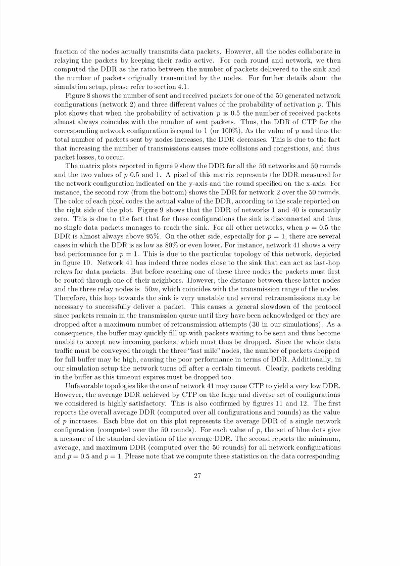
fraction of the nodes actually transmits data packets. However, all the nodes collaborate inrelaying the packets by keeping their radio active. For each round and network, we thencomputed the DDR as the ratio between the number of packets delivered to the sink andthe number of packets originally transmitted by the nodes. For further details about thesimulation setup, please refer to section 4.1.
Figure 8 shows the number of sent and received packets for one of the 50 generated networkconfigurations (network 2) and three different values of the probability of activation p. Thisplot shows that when the probability of activation p is 0.5 the number of received packetsalmost always coincides with the number of sent packets. Thus, the DDR of CTP for thecorresponding network configuration is equal to 1 (or 100%). As the value of p and thus thetotal number of packets sent by nodes increases, the DDR decreases. This is due to the factthat increasing the number of transmissions causes more collisions and congestions, and thuspacket losses, to occur.
The matrix plots reported in figure 9 show the DDR for all the 50 networks and 50 roundsand the two values of p 0.5 and 1. A pixel of this matrix represents the DDR measured forthe network configuration indicated on the y-axis and the round specified on the x-axis. Forinstance, the second row (from the bottom) shows the DDR for network 2 over the 50 rounds.
The color of each pixel codes the actual value of the DDR, according to the scale reported onthe right side of the plot. Figure 9 shows that the DDR of networks 1 and 40 is constantlyzero. This is due to the fact that for these configurations the sink is disconnected and thusno single data packets manages to reach the sink. For all other networks, when p = 0.5 theDDR is almost always above 95%. On the other side, especially for p = 1, there are severalcases in which the DDR is as low as 80% or even lower. For instance, network 41 shows a verybad performance for p = 1. This is due to the particular topology of this network, depictedin figure 10. Network 41 has indeed three nodes close to the sink that can act as last-hoprelays for data packets. But before reaching one of these three nodes the packets must firstbe routed through one of their neighbors. However, the distance between these latter nodesand the three relay nodes is 50m, which coincides with the transmission range of the nodes.
Therefore, this hop towards the sink is very unstable and several retransmissions may benecessary to successfully deliver a packet. This causes a general slowdown of the protocolsince packets remain in the transmission queue until they have been acknowledged or they aredropped after a maximum number of retransmission attempts (30 in our simulations). As aconsequence, the buffer may quickly fill up with packets waiting to be sent and thus becomeunable to accept new incoming packets, which must thus be dropped. Since the whole datatraffic must be conveyed through the three “last mile” nodes, the number of packets droppedfor full buffer may be high, causing the poor performance in terms of DDR. Additionally, inour simulation setup the network turns off after a certain timeout. Clearly, packets residingin the buffer as this timeout expires must be dropped too.
Unfavorable topologies like the one of network 41 may cause CTP to yield a very low DDR.
However, the average DDR achieved by CTP on the large and diverse set of configurationswe considered is highly satisfactory. This is also confirmed by figures 11 and 12. The firstreports the overall average DDR (computed over all configurations and rounds) as the valueof p increases. Each blue dot on this plot represents the average DDR of a single networkconfiguration (computed over the 50 rounds). For each value of p, the set of blue dots givea measure of the standard deviation of the average DDR. The second reports the minimum,average, and maximum DDR (computed over the 50 rounds) for all network configurationsand p = 0.5 and p = 1. Please note that we compute these statistics on the data corresponding
27
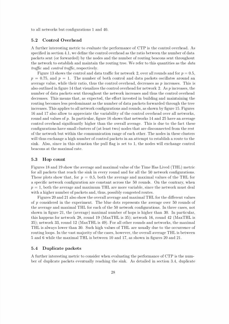
8/4/2019 CTP Over Castalia
http://slidepdf.com/reader/full/ctp-over-castalia 28/47

8/4/2019 CTP Over Castalia
http://slidepdf.com/reader/full/ctp-over-castalia 29/47
packets are generated when acknowledgments get lost or are not received within a given time-out. Figure 22 shows the number of duplicate packets for all network configurations androunds, while figure 23 shows the corresponding average for each network and over all net-works as p increases. As expected, the number of duplicate packets increases as the value of p increases. The presence of duplicate packets clearly contributes to congest the network and
thus negatively affects the performance of CTP.
6 Conclusions
This reports provides a detailed description of the implementation of the Collection Tree Pro-tocol for the Castalia wireless sensor networks simulator. The report focuses on particularlytricky implementation issues and represents an handy reference for other researchers inter-ested in working with CTP or re-implementing it for other platforms. The validity of theimplementation has been tested through an extensive simulation study, which also confirmedthe convincing performance of CTP in terms of data delivery ratio.
29
8/4/2019 CTP Over Castalia
http://slidepdf.com/reader/full/ctp-over-castalia 30/47
References
[1] I. F. Akyildiz, W. Su, Y. Sankarasubramaniam, and E. Cayirci. Wireless Sensor Networks:A Survey. Computer Networks , 38(4):393–422, March 2002.
[2] Athanassios Boulis et al. Castalia: A Simulator for Wireless Sensor Networks. http:
//castalia.npc.nicta.com.au/.
[3] Aline Baggio. Wireless Sensor Networks in Precision Agriculture. In Proceedings of the First Workshop on Real-World Wireless Sensor Networks (REALWSN 2005), Stockholm,Sweden, June 2005.
[4] Manohar Bathula, Mehrdad Ramezanali, Ishu Pradhan, Nilesh Patel, Joe Gotschall, andNigamanth Sridhar. A Sensor Network System for Measuring Traffic in Short-Term Con-struction Work Zones. In Proceedings of the 5th IEEE International Conference on Dis-tributed Computing in Sensor Systems (DCOSS 2009), pages 216–230, Marina del Rey,CA, USA, Berlin, Heidelberg, 2009. Springer-Verlag.
[5] Lorenzo Bergamini, Carlo Crociani, and Andrea Vitaletti. Simulation vs Real Testbeds:A Validation of WSN Simulators. Technical Report 3, Sapienza Università di Roma,Dipartimento di Informatica e Sistemistica Antonio Ruberti, 2009.
[6] Athanassios Boulis. Castalia User Manual (version 1.3). http://castalia.npc.nicta.
com.au/pdfs/Castalia%20-%20User%20Manual.pdf.
[7] Athanassios Boulis. Castalia: Revealing Pitfalls in Designing Distributed Algorithmsin WSN. In Proceedings of the 5th International Conference on Embedded Networked Sensor Systems (SenSys 2007), pages 407–408, Sydney, Australia, 6-7 November 2007.Demonstration session.
[8] Athanassios Boulis, Ansgar Fehnker, Matthias Fruth, and Annabelle McIver. CaVi –Simulation and Model Checking forWireless Sensor Networks. In Proceedings of the Fifth International Conference on Quantitative Evaluation of Systems (QEST 2008), pages37–38, Saint Malo, France, September 14-17 2008.
[9] Phil Buonadonna, David Gay, Joseph M. Hellerstein, Wei Hong, and Samuel Madden.TASK: Sensor Network in a Box. In Proceedings of the 2nd IEEE European Workshop on Wireless Sensor Networks and Applications (EWSN 2005), Istanbul, Turkey, February2005.
[10] Nicolas Burri, Pascal von Rickenbach, and Roger Wattenhofer. Dozer: Ultra-Low PowerData Gathering in Sensor Networks. In Proceedings of the 6th International Conference on Information Processing in Sensor Networks (IPSN 2007), Cambridge, MA, USA, April2007.
[11] ChipCon 2420 Datasheet. http://focus.ti.com/lit/ds/symlink/cc2420.pdf.
[12] Crossbow Technology Inc. www.xbow.com.
[13] J. E. Egea-López, A. Vales-Alonso, P. S. Martínez-Sala, J. Pavón-Mario, and García-Haro. Simulation Tools for Wireless Sensor Networks. In International Symposium on
30

8/4/2019 CTP Over Castalia
http://slidepdf.com/reader/full/ctp-over-castalia 31/47
Performance Evaluation of Computer and Telecommunication Systems (SPECTS 2005),Philadelphia, PA, USA, July 2005.
[14] Deborah Estrin, Ramesh Govindan, John Heidemann, and Satish Kumar. Next CenturyChallenges: Scalable Coordination in Sensor Networks. In Proceedings of the 5th annual ACM/IEEE International Conference on Mobile Computing and Networking (Mobicom
1999), pages 263 – 270, Seattle, WA, USA, 1999.
[15] Rodrigo Fonseca, Omprakash Gnawali, Kyle Jamieson, Sukun Kim, Philip Levis, andAlec Woo. TinyOS Enhancement Proposal (TEP) 123: The Collection Tree Protocol(CTP). www.tinyos.net/tinyos-2.x/doc/pdf/tep123.pdf.
[16] Rodrigo Fonseca, Omprakash Gnawali, Kyle Jamieson, and Philip Levis. TinyOS En-hancement Proposal (TEP) 119: Collection. www.tinyos.net/tinyos-2.x/doc/pdf/
tep119.pdf.
[17] Omprakash Gnawali, Rodrigo Fonseca, Kyle Jamieson, and Philip Levis. CTP: Robustand Efficient Collection through Control and Data Plane Integration. Technical report,The Stanford Information Networks Group (SING), 2008. http://sing.stanford.edu/
pubs/sing-08-02.pdf.
[18] Omprakash Gnawali, Rodrigo Fonseca, Kyle Jamieson, David Moss, and Philip Levis.Collection Tree Protocol. In Proceedings of the 7th ACM Conference on Embedded Net-worked Sensor Systems (SenSys 2009), Berkeley, CA, USA, November 2009.
[19] Miloš Jevtić, Nikola Zogović, and Goran Dimić. Evaluation of Wireless Sensor NetworkSimulators. In Proceedings of the 17th Telecommunications Forum (TELFOR 2009),Belgrade, Serbia, November 2009.
[20] Holger Karl and Andreas Willig. Protocols and Architectures for Wireless Sensor Net-works . John Wiley and Sons, 2005.
[21] Alireza Khadivi and Martin Hasler. Fire Detection and Localization Using WirelessSensor Networks. Sensor Applications Experimentation and Logistics , 29:16–26, 2010.
[22] JeongGil Ko, Tia Gao, and Andreas Terzis. Empirical Study of a Medical Sensor Ap-plication in an Urban Emergency Department. In Proceedings of the 4th International Conference on Body Area Networks (BodyNets 2009), Los Angeles, CA, USA, April 2009.
[23] Philip Levis. TinyOS Enhancement Proposal (TEP) 116: Packet Protocols. www.tinyos.net/tinyos-2.x/doc/pdf/tep116.pdf.
[24] Philip Levis, Neil Patel, David Culler, and Scott Shenker. A Self-Regulating Algorithmfor Code Maintenance and Propagation in Wireless Sensor Networks. In Proceedings of
the 1st USENIX Conference on Networked Systems Design and Implementation (NSDI 2004), San Francisco, CA, USA, March 2004.
[25] Philipp Levis and David Gay. TinyOS Programming . Cambridge University Press, 2009.
[26] Andreas Meier, Mehul Motani, Hu Siquan, and Simon Künzli. DiMo: Distributed NodeMonitoring in Wireless Sensor Networks. In Proceedings of the 11th International Sym-posium on Modeling, Analysis and Simulation of Wireless and Mobile Systems (MSWiM 2008), pages 117–121, Vancouver, Canada, New York, NY, USA, October 2008. ACM.
31
8/4/2019 CTP Over Castalia
http://slidepdf.com/reader/full/ctp-over-castalia 32/47
[27] Andreas Meier, Matthias Woehrle, Mischa Weise, Jan Beutel, and Lothar Thiele. NoSE:Efficient Maintenance and Initialization of Wireless Sensor Networks. In Proceedings of the 6th Annual IEEE Communications Society Conference on Sensor, Mesh and Ad Hoc Communications and Networks (SECON 2009 , pages 395–403, Rome, Italy, Piscataway,NJ, USA, 2009. IEEE Press.
[28] David Moss, Jonathan Hui, Philip Levis, and Jung Il Choi. TinyOS Enhancement Pro-posal (TEP) 126: CC2420 Radio Stack. www.tinyos.net/tinyos-2.x/doc/pdf/tep126.pdf.
[29] OMNeT++ User Manual (Version 3.2). www.omnetpp.org/doc/omnetpp33/manual/usman.html.
[30] Sung Park, Andreas Savvides, and Mani B. Srivastava. SensorSim: a Simulation Frame-work for Sensor Networks. In Proceedings of the 3rd ACM International Workshop on Modeling, Analysis and Simulation of Wireless and Mobile Systems (MSWiM 2000), pages104–111, Boston, MA, USA, August 2000.
[31] Hai N. Pham, Dimosthenis Pediaditakis, and Athanassios Boulis. From Simulation to Real
Deployments in WSN and Back. In Proceedings of the IEEE International Symposium on a World of Wireless, Mobile and Multimedia Networks (WoWMoM 2007) , pages 1–6,Helsinki, Finland, June 18-21 2007.
[32] Joseph Polastre, Robert Szewczyk, and David Culler. Telos: Enabling Ultra-Low PowerWireless Research. In Proceedings of the 4th International Conference on Information Processing in Sensor Networks: Special track on Platform Tools and Design Methods for Network Embedded Sensors (IPSN/SPOTS 2005), pages 364–369, Los Angeles, CA, USA,April 2005.
[33] Thomas Schmid, Zainul Charbiwala, Roy Shea, and Mani Srivastava. Temperature Com-pensated Time Synchronization. IEEE Embedded Systems Letters (ESL), 1(2):37–41,
August 2009.
[34] Robert Szewczyk, Alan Mainwaring, Joseph Polastre, John Anderson, and David Culler.An Analysis of a Large Scale Habitat Monitoring Application. In Proceedings of the Second ACM Conference on Embedded Networked Sensor Systems (SenSys 2004), Baltimore, MD,USA, November 2004.
[35] Igor Talzi, Andreas Hasler, Stephan Gruber, and Christian Tschudin. PermaSense: In-vestigating Permafrost with a WSN in the Swiss Alps. In Proceedings of the Fourth ACM Workshop on Embedded Networked Sensors (EmNets 2007), Cork, Ireland, June 2007.
[36] Simon Tschirner, Liang Xuedong, and Wang Yi. Model-based Validation of QoS Proper-
ties of Biomedical Sensor Networks. In Proceedings of the 8th ACM International Con- ference On Embedded Software , pages 69–78, Atlanta, GA, USA, October 2008.
[37] Tijs van Dam and Koen Langendoen. An Adaptive Energy-Efficient MAC Protocol forWireless Sensor Networks. In Proceedings of the First International Conference on Em-bedded Networked Sensing Systems (SenSys 2003), pages 171 – 180, New York, NY, USA,2003.
32

8/4/2019 CTP Over Castalia
http://slidepdf.com/reader/full/ctp-over-castalia 33/47
[38] Alec Woo, Terence Tong, and David Culler. Taming the Underlying Challenges of ReliableMultihop Routing in Sensor Networks. In Proceedings of the 1st ACM International Conference on Embedded Networked Sensor Systems (SenSys 2003), pages 14–27, LosAngeles, CA, USA, November 2003.
33
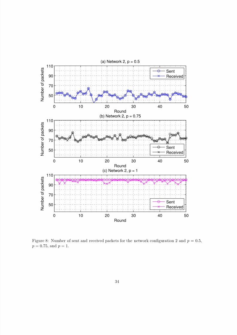
8/4/2019 CTP Over Castalia
http://slidepdf.com/reader/full/ctp-over-castalia 34/47
0 10 20 30 40 50
50
70
90
110
Round
N u m b e r o f p a c k e t s
(a) Network 2, p = 0.5
Sent
Received
0 10 20 30 40 50
50
70
90
110
Round
N u m b e r o f p a c k e t s
(b) Network 2, p = 0.75
Sent
Received
0 10 20 30 40 50
50
70
90
110
Round
N u m b e r o f p a c k e t s
(c) Network 2, p = 1
Sent
Received
Figure 8: Number of sent and received packets for the network configuration 2 and p = 0.5, p = 0.75, and p = 1.
34

8/4/2019 CTP Over Castalia
http://slidepdf.com/reader/full/ctp-over-castalia 35/47
0 5 10 15 20 25 30 35 40 45 500
5
10
15
20
25
30
35
40
45
50
Round
N e t w o r k c o n f i g u r a t i o n
Data Delivery Ratio for p = 0.5
0
0.1
0.2
0.3
0.4
0.5
0.6
0.7
0.8
0.9
1
0 5 10 15 20 25 30 35 40 45 500
5
10
15
20
25
30
35
40
45
50
Round
N e t w o r k c o n f i g u r a t i o n
Data Delivery Ratio for p = 1
0
0.1
0.2
0.3
0.4
0.5
0.6
0.7
0.8
0.9
1
Figure 9: DDR for all the network configurations and rounds, for p = 0.5 and p = 1.
35

8/4/2019 CTP Over Castalia
http://slidepdf.com/reader/full/ctp-over-castalia 36/47
−50 0 50 100 150 200 250 300−50
0
50
100
150
200
250
300
x
y
Topology of network 41
Sink
Nodes
Figure 10: Physical topology of network configuration no 41.
0.5 0.55 0.6 0.65 0.7 0.75 0.8 0.85 0.9 0.95 10
0.1
0.2
0.3
0.4
0.5
0.6
0.7
0.8
0.9
1
1.1Average data delivery ratio
Probability of activation p
D a t a d e l i v e r y r a t i o
Figure 11: Average data delivery ratio for all networks and values of p.
36

8/4/2019 CTP Over Castalia
http://slidepdf.com/reader/full/ctp-over-castalia 37/47
1
2
3
4
5
6
7
8
9
1 0
1 1
1 2
1 3
1 4
1 5
1 6
1 7
1 8
1 9
2 0
2 1
2 2
2 3
2 4
2 5
2 6
2 7
2 8
2 9
3 0
3 1
3 2
3 3
3 4
3 5
3 6
3 7
3 8
3 9
4 0
4 1
4 2
4 3
4 4
4 5
4 6
4 7
4 8
4 9
5 0
0 0 . 2
0 . 4
0 . 6
0 . 8 1
1 . 2
M i n i m u m , a v e r a g e , a n d m a x i m u m d
a t a d e l i v e r
y r a t i o , p = 0 . 5
N e t w o r k c o n f i g u r a t i o n
D a t a d e l i v e r y r a t i o
M i n i m u m
A v e r a g e
M a x i m u m
1
2
3
4
5
6
7
8
9
1 0
1 1
1 2
1 3
1 4
1 5
1 6
1 7
1 8
1 9
2 0
2 1
2 2
2 3
2 4
2 5
2 6
2 7
2 8
2 9
3 0
3 1
3 2
3 3
3 4
3 5
3 6
3 7
3 8
3 9
4 0
4 1
4 2
4 3
4 4
4 5
4 6
4 7
4 8
4 9
5 0
0 0 . 2
0 . 4
0 . 6
0 . 8 1
M i n i m u m , a v e r a g e , a n d m a x i m u m d
a t a d e l i v e
r y r a t i o , p = 1
N e t w o r k c o n f i g u r a t i o n
D a t a d e l i v e r y r a t i o
M i n i m u m
A v e r a g e
M a x i m u m
Figure 12: Minimum, average, and maximum data delivery ratio for all networks and p = 0.5and p = 1.
37

8/4/2019 CTP Over Castalia
http://slidepdf.com/reader/full/ctp-over-castalia 38/47
0 10 20 30 40 500
500
1000
1500
2000
Round
N u m b e r o f p a c k e t s
Network 2, p = 0.5
Control
Data
0 10 20 30 40 500
500
1000
1500
2000
Round
N u m b e r o f p a c k e t s
Network 2, p = 0.75
ControlData
0 10 20 30 40 50
0
500
1000
1500
2000
Round
N u m b e r o f p a c k e t s
Network 2, p = 1
Control
Data
Figure 13: Number of control and data packets sent throughout network 2 for p = 0.5, p = 0.75, and p = 1.
38

8/4/2019 CTP Over Castalia
http://slidepdf.com/reader/full/ctp-over-castalia 39/47
5 10 15 20 25 30 35 40 45 500
1
2
3
4
5
6
Round
C o n t r o l o v e r h e a d
Network 2, p = 0.5
5 10 15 20 25 30 35 40 45 500
1
2
3
4
5
6
Round
C o n t r o l o v e r h e a d
Network 2, p = 0.75
5 10 15 20 25 30 35 40 45 500
1
2
3
4
5
6
Round
C o n t r o l o v e r h e a d
Network 2, p = 1
Figure 14: Control overhead for network 2 for p = 0.5, p = 0.75, and p = 1.
39

8/4/2019 CTP Over Castalia
http://slidepdf.com/reader/full/ctp-over-castalia 40/47
0 5 10 15 20 25 30 35 40 45 500
5
10
15
20
25
30
35
40
45
50
round
n e t w o r k c o n f i g u r a t i o n
Control overhead for p=0.5
0
1
2
3
4
5
6
7
0 5 10 15 20 25 30 35 40 45 500
5
10
15
20
25
30
35
40
45
50
round
n e t w o r k c o n f i g u r a t i o n
Control overhead for p = 1
0
1
2
3
4
5
6
7
Figure 15: Control overhead for all networks and rounds, for p = 0.5 and p = 1.
40
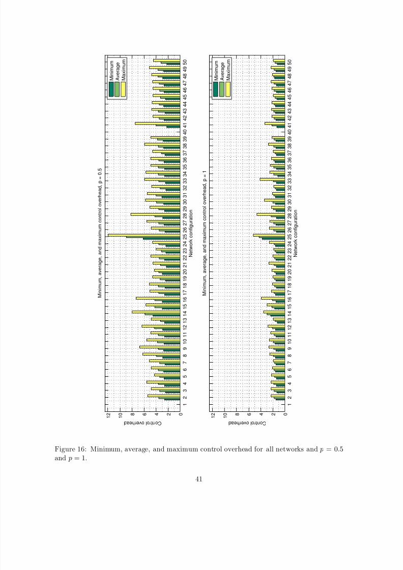
8/4/2019 CTP Over Castalia
http://slidepdf.com/reader/full/ctp-over-castalia 41/47
1
2
3
4
5
6
7
8
9
1 0 1 1 1 2 1 3 1 4 1 5 1 6
1 7 1 8 1 9 2 0 2 1 2 2 2 3 2 4 2 5 2 6 2 7 2 8 2 9 3 0
3 1 3 2 3 3 3 4 3 5 3 6 3 7 3 8 3 9 4 0 4 1 4 2 4 3 4 4 4
5 4 6 4 7 4 8 4 9 5 0
0 2 4 6 8 1 0
1 2
M i n i m u m , a v e r a g e , a n d m a x i m u m c
o n t r o l o v e
r h e a d , p = 0 . 5
N e t w o r k c o n f i g u r a t i o n
C o n t r o l o v e r h e a d
M i n i m u m
A v e r a g e
M a x i m u m
1
2
3
4
5
6
7
8
9
1 0 1 1 1 2 1 3 1 4 1 5 1 6
1 7 1 8 1 9 2 0 2 1 2 2 2 3 2 4 2 5 2 6 2 7 2 8 2 9 3 0
3 1 3 2 3 3 3 4 3 5 3 6 3 7 3 8 3 9 4 0 4 1 4 2 4 3 4 4 4
5 4 6 4 7 4 8 4 9 5 0
0 2 4 6 8 1 0
1 2
M i n i m u m , a v e r a g e , a n d m a x i m u m c
o n t r o l o v e r h e a d , p = 1
N e t w o r k c o n f i g u r a t i o n
C o n t r o l o v e r h e a d
M i n i m u m
A v e r a g e
M a x i m u m
Figure 16: Minimum, average, and maximum control overhead for all networks and p = 0.5and p = 1.
41
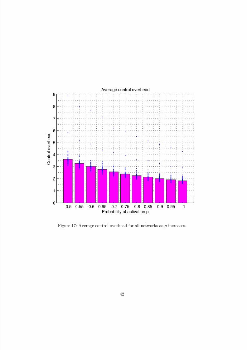
8/4/2019 CTP Over Castalia
http://slidepdf.com/reader/full/ctp-over-castalia 42/47
0.5 0.55 0.6 0.65 0.7 0.75 0.8 0.85 0.9 0.95 10
1
2
3
4
5
6
7
8
9Average control overhead
Probability of activation p
C o n t r o l o v e r h e a d
Figure 17: Average control overhead for all networks as p increases.
42

8/4/2019 CTP Over Castalia
http://slidepdf.com/reader/full/ctp-over-castalia 43/47
0 5 10 15 20 25 30 35 40 45 500
5
10
15
20
25
30
35
40
45
50
Round
N e t w o r k c o n f i g u r a t i o n
Average number of hops for p = 0.5
0
1
2
3
4
5
6
7
8
9
10
0 5 10 15 20 25 30 35 40 45 500
5
10
15
20
25
30
35
40
45
50
Round
N e t w o r k c o n f i g u r a t i o n
Average number of hops for p = 1
0
1
2
3
4
5
6
7
8
9
10
Figure 18: Average THL for all the network configurations and rounds and p = 0.5 and p = 1.
43

8/4/2019 CTP Over Castalia
http://slidepdf.com/reader/full/ctp-over-castalia 44/47
0 5 10 15 20 25 30 35 40 45 500
5
10
15
20
25
30
35
40
45
50
Round
N e t w o r k c o n f i g u r a t i o n
Maximum number of hops for p = 0.5
5
10
15
20
25
30
0 5 10 15 20 25 30 35 40 45 500
5
10
15
20
25
30
35
40
45
50
Round
N e t w o r k c o n f i g u r a t i o n
Maximum number of hops for p = 1
5
10
15
20
25
30
Figure 19: Maximum THL for all the network configurations and rounds and p = 0.5 and p = 1.
44

8/4/2019 CTP Over Castalia
http://slidepdf.com/reader/full/ctp-over-castalia 45/47
0.5 0.55 0.6 0.65 0.7 0.75 0.8 0.85 0.9 0.95 1
1
2
3
4
5
6
7
8Average number of hops
Probability of activation p
N u m b e r o f h o p s
Figure 20: Average THL for all networks as p increases.
0.5 0.55 0.6 0.65 0.7 0.75 0.8 0.85 0.9 0.95 10
2
4
6
8
10
12
14
16
18
20
22
24
26
28
30Maximum number of hops
Probability of activation p
N u m b e r o f h o p s
Figure 21: Maximum THL for all networks as p increases.
45

8/4/2019 CTP Over Castalia
http://slidepdf.com/reader/full/ctp-over-castalia 46/47
0 5 10 15 20 25 30 35 40 45 500
5
10
15
20
25
30
35
40
45
50
Round
N e t w o r k c o n f i g u r a t i o n
Number of duplicate packets for p = 0.5
0
5
10
15
20
25
30
35
40
45
50
55
0 5 10 15 20 25 30 35 40 45 500
5
10
15
20
25
30
35
40
45
50
Round
N e t w o r k c o n f i g u r a t i o n
Number of duplicate packets for p = 1
0
5
10
15
20
25
30
35
40
45
50
55
Figure 22: Number of duplicate packets for all the network configurations and rounds for p = 0.5 and p = 1.
46
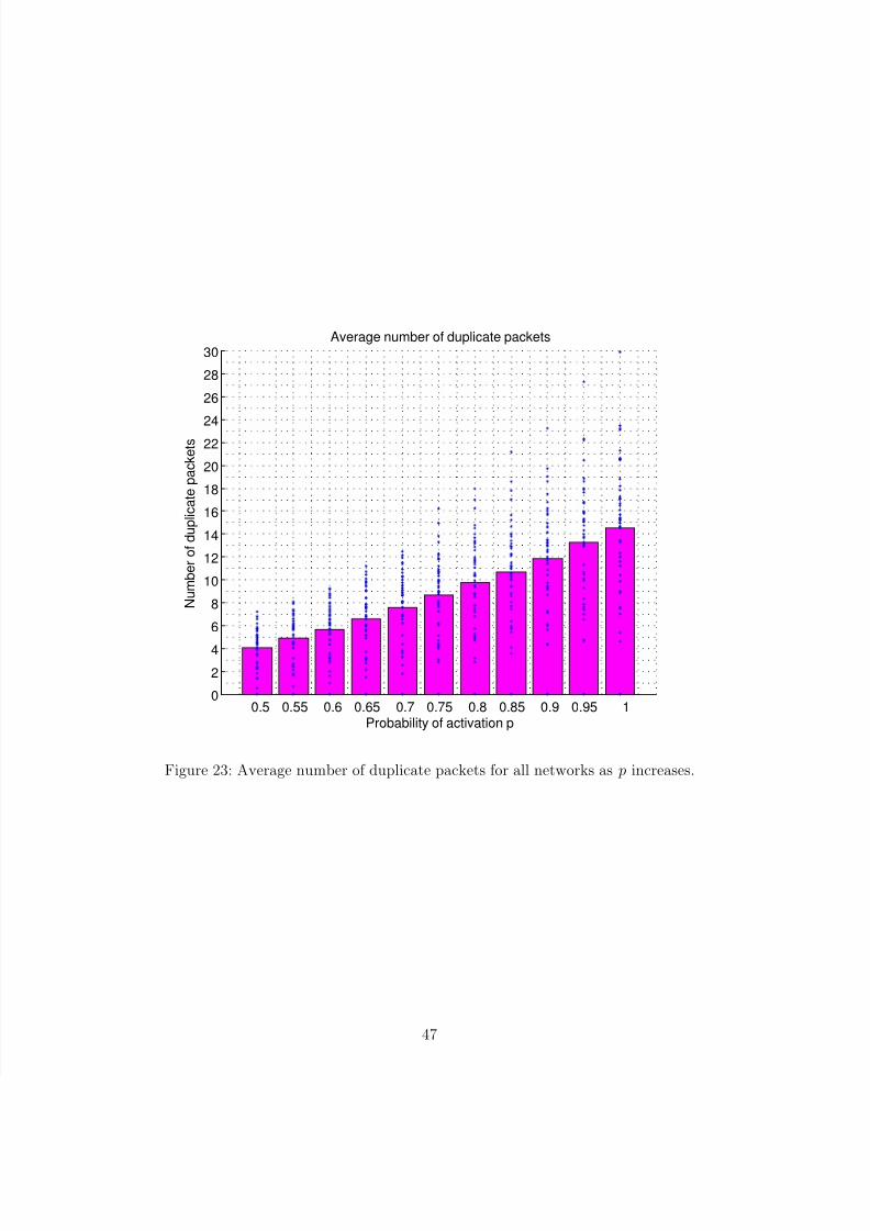
8/4/2019 CTP Over Castalia
http://slidepdf.com/reader/full/ctp-over-castalia 47/47
0.5 0.55 0.6 0.65 0.7 0.75 0.8 0.85 0.9 0.95 10
2
4
6
8
10
12
14
16
18
20
22
24
26
28
30Average number of duplicate packets
Probability of activation p
N u m b e r o f d u p l i c a t e p a c k e t s
Figure 23: Average number of duplicate packets for all networks as p increases.