Embed Size (px)
Citation preview

Faculty of Actuaries Institute of Actuaries
EXAMINATION
14 April 2005 (am)
Subject CT6 Statistical Methods Core Technical
Time allowed: Three hours
INSTRUCTIONS TO THE CANDIDATE
1. Enter all the candidate and examination details as requested on the front of your answer booklet.
2. You must not start writing your answers in the booklet until instructed to do so by the supervisor.
3. Mark allocations are shown in brackets.
4. Attempt all 10 questions, beginning your answer to each question on a separate sheet.
5. Candidates should show calculations where this is appropriate.
Graph paper is not required for this paper.
AT THE END OF THE EXAMINATION
Hand in BOTH your answer booklet, with any additional sheets firmly attached, and this question paper.
In addition to this paper you should have available the 2002 edition of the Formulae and Tables and your own electronic calculator.
Faculty of Actuaries CT6 A2005 Institute of Actuaries

CT6 A2005 2
1 List the three main perils typically covered by employer s liability insurance. [3]
2 An insurer wishes to estimate the expected number of claims, , on a particular type of policy. Prior beliefs about are represented by a Gamma distribution with density function
f( ) = ( )
1 e ( > 0).
For an estimate, d, of the loss function is defined as
L( , d) = (
d)2 + d2.
Show that the expected loss is given by
E(L( , d)) = 22
( 1) 22
dd
and hence determine the optimal estimate for under the Bayes rule. [5]
3 (i) Explain the disadvantages of using truly random, as opposed to pseudo-random, numbers. [3]
(ii) List four methods for the generation of random variates. [2] [Total 5]
4 Yt, t = 1, 2, 3, is a time series defined by
Yt 0.8Yt 1 = Zt + 0.2Zt 1
where Zt, t = 0, 1, is a sequence of independent zero-mean variables with common
variance 2.
Derive the autocorrelation k, k = 0, 1, 2,
[6]
CT6 A2005 3 PLEASE TURN OVER
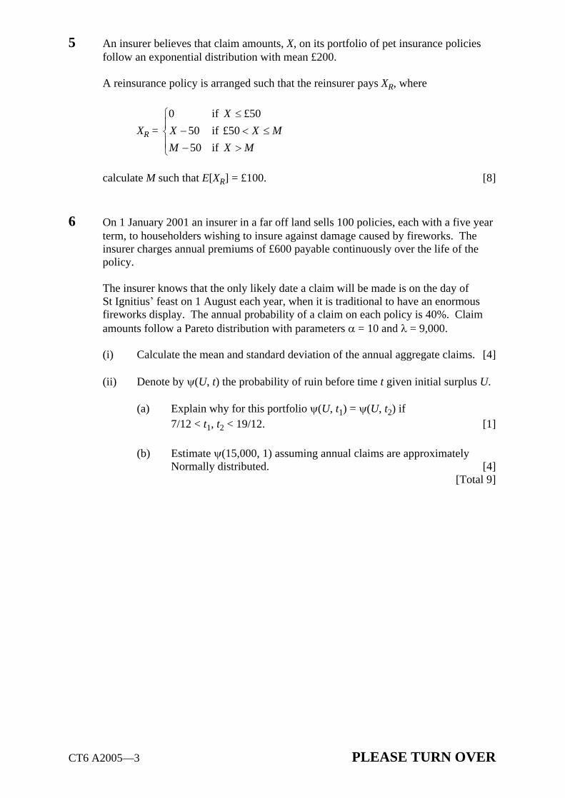
5 An insurer believes that claim amounts, X, on its portfolio of pet insurance policies follow an exponential distribution with mean £200.
A reinsurance policy is arranged such that the reinsurer pays XR, where
XR =
0 if £50
50 if £50
50 if
X
X X M
M X M
calculate M such that E[XR] = £100. [8]
6 On 1 January 2001 an insurer in a far off land sells 100 policies, each with a five year term, to householders wishing to insure against damage caused by fireworks. The insurer charges annual premiums of £600 payable continuously over the life of the policy.
The insurer knows that the only likely date a claim will be made is on the day of St Ignitius feast on 1 August each year, when it is traditional to have an enormous fireworks display. The annual probability of a claim on each policy is 40%. Claim amounts follow a Pareto distribution with parameters = 10 and = 9,000.
(i) Calculate the mean and standard deviation of the annual aggregate claims. [4]
(ii) Denote by (U, t) the probability of ruin before time t given initial surplus U.
(a) Explain why for this portfolio (U, t1) = (U, t2) if 7/12 < t1, t2 < 19/12. [1]
(b) Estimate (15,000, 1) assuming annual claims are approximately Normally distributed. [4]
[Total 9]

CT6 A2005 4
7 The no claims discount (NCD) system operated by an insurance company has three levels of discount: 0%, 25% and 50%.
If a policyholder makes a claim they remain at or move down to the 0% discount level for two years. Otherwise they move up a discount level in the following year or remain at the maximum 50% level.
The probability of an accident depends on the discount level:
Discount Level Probability of accident
0% 0.25 25% 0.2 50% 0.1
The full premium payable at the 0% discount level is 750.
Losses are assumed to follow a lognormal distribution with mean 1,451 and standard deviation 604.4.
Policyholders will only claim if the loss is greater than the total additional premiums that would have to be paid over the next three years, assuming that no further accidents occur.
(i) Calculate the smallest loss for which a claim will be made for each of the four states in the NCD system. [2]
(ii) Determine the transition matrix for this NCD system. [6]
(iii) Calculate the proportion of policyholders at each discount level when the system reaches a stable state. [3]
(iv) Determine the average premium paid once the system reaches a stable state.[1]
(v) Describe the limitations of simple NCD systems such as this one. [2] [Total 14]
8 (i) Write down the general form of a statistical model for a claims run-off triangle, defining all terms used. [5]
(ii) The table below shows the cumulative incurred claims on a portfolio of insurance policies.
Accident Year Delay Year
2000 2,748 3,819 3,991 2001 2,581 4,014 2002 3,217

CT6 A2005 5 PLEASE TURN OVER
The company decides to apply the Bornhuetter-Ferguson method to calculate the reserves, with the assumption that the Ultimate Loss Ratio is 85%.
Calculate the reserve for 2002, if the earned premium is 5,012 and the paid claims are 1,472. [9]
[Total 14]
9 Y1, Y2, , Yn are independent claims, which are assumed to be exponentially distributed, with
E[Yi] = i .
(i) Show that the canonical link function is the inverse link function. [3]
(ii) It is decided that the canonical link function should not be used, but that the mean claim sizes should be modelled as follows:
log i = 1, 2, ...,
1, 2, ...,
i m
i m m n
(a) Show that the log-likelihood can be written as
1 1
( )m n
i ii i m
m n m e y e y
(b) Derive the maximum likelihood estimators of and .
(c) Show that the scaled deviance for this model is
1 1
1 1
1 1
2 log log
m n
j jm nj j m
i ii i m
y ym n m
y y
[12]
(iii) For a particular data set, m = 20, n = 44,
20 44
1 21
1 1= 14.2, = 18.7.
20 24i ii i
y y
Calculate the deviance residual for y1 = 7. [3] [Total 18]

CT6 A2005 6
10 (i) Explain what a conjugate prior distribution is. [2]
(ii) The random variables X1, X2, , Xn are independent and have density function
f(x) = e x (x > 0).
Show that the conjugate prior distribution for is a Gamma distribution. [3]
(iii) (a) The density function of is
f( ) = 1
( )ss
e ( > 0).
Show that E(1/ ) = s/(
1).
(b) Hence if X1, X2, , Xn is an independent random sample from an
exponential distribution with parameter , show that the posterior mean of 1/ can be expressed as a weighted average of the prior mean of 1/ and the sample average.
[5]
(iv) An insurer is considering introducing a new policy to provide insurance against the failure of toasters within the first five years of purchase. Alan and Beatrice are underwriters working for the insurer. Based on his experience of similar products, Alan believes that toasters last three years on average. Beatrice believes that six years is the average lifetime. Both are adamant and are prepared to express their uncertainties about the average lifetime in terms of standard deviations of six months and one year respectively. They decide to resolve their differences by testing a sample of toasters large enough to ensure the difference in their posterior expectations for the average lifetime will be less than one year.
Calculate how many toasters they should test, assuming the exponential distribution is a good model for toaster lifetimes.
You may use the fact that if ~ ( , s) then
Var(1/ ) = [E(1/ )]2
1.
2
[8]
[Total 18]
END OF PAPER

Faculty of Actuaries Institute of Actuaries
EXAMINATION
April 2005
Subject CT6 Statistical Methods Core Technical
EXAMINERS REPORT
Introduction
The attached subject report has been written by the Principal Examiner with the aim of helping candidates. The questions and comments are based around Core Reading as the interpretation of the syllabus to which the examiners are working. They have however given credit for any alternative approach or interpretation which they consider to be reasonable.
M Flaherty
Chairman of the Board of Examiners
15 June 2005
Faculty of Actuaries Institute of Actuaries
Subject CT6 (Statistical Methods Core Technical) April 2005
Examiners Report
Page 2
1 The three main perils are:
accidents caused by the negligence of the employer or other employees
exposure to harmful substances
exposure to harmful working conditions
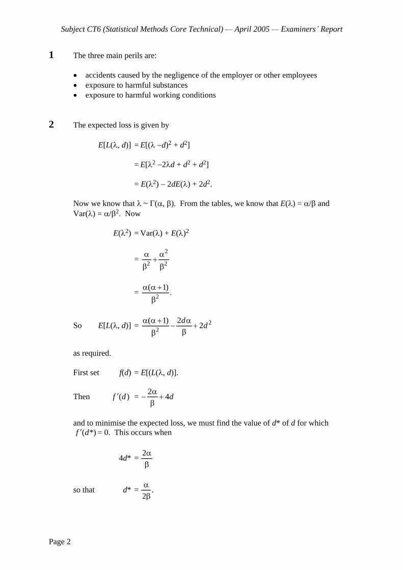
2 The expected loss is given by
E[L( , d)] = E[(
d)2 + d2]
= E[ 2 2 d + d2 + d2]
= E( 2) 2dE( ) + 2d2.
Now we know that ~ ( , ). From the tables, we know that E( ) = / and Var( ) = / 2. Now
E( 2) = Var( ) + E( )2
= 2
2 2
= 2
( 1).
So E[L( , d)] = 22
( 1) 22
dd
as required.
First set f(d) = E[(L( , d)].
Then ( )f d
= 2
4d
and to minimise the expected loss, we must find the value of d* of d for which ( *)f d = 0. This occurs when
4d* = 2
so that d* = .2
Subject CT6 (Statistical Methods Core Technical) April 2005
Examiners Report
Page 3
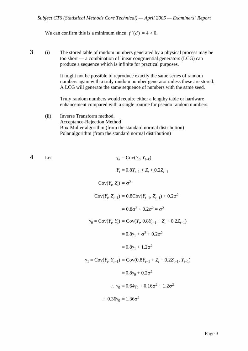
We can confirm this is a minimum since ( )f d = 4 > 0.
3 (i) The stored table of random numbers generated by a physical process may be too short a combination of linear congruential generators (LCG) can produce a sequence which is infinite for practical purposes.
It might not be possible to reproduce exactly the same series of random numbers again with a truly random number generator unless these are stored. A LCG will generate the same sequence of numbers with the same seed.
Truly random numbers would require either a lengthy table or hardware enhancement compared with a single routine for pseudo random numbers.
(ii) Inverse Transform method. Acceptance-Rejection Method Box-Muller algorithm (from the standard normal distribution) Polar algorithm (from the standard normal distribution)
4 Let k = Cov(Yt, Yt k)
Yt = 0.8Yt 1 + Zt + 0.2Zt 1
Cov(Yt, Zt) = 2
Cov(Yt, Zt 1) = 0.8Cov(Yt 1, Zt 1) + 0.2 2
= 0.8 2 + 0.2 2 = 2
0 = Cov(Yt, Yt) = Cov(Yt, 0.8Yt 1 + Zt + 0.2Zt 1)
= 0.8 1 + 2 + 0.2 2
= 0.8 1 + 1.2 2
1 = Cov(Yt, Yt 1) = Cov(0.8Yt 1 + Zt + 0.2Zt 1, Yt 1)
= 0.8 0 + 0.2 2
0 = 0.64 0 + 0.16 2 + 1.2 2
0.36 0 = 1.36 2

Subject CT6 (Statistical Methods Core Technical) April 2005
Examiners Report
Page 4
0 = 21.36
0.36
= 3.78 2
1 = 3.22 2
For k 2, k = Cov(Yt, Yt k) = 0.8 k 1
The autocorrelation function is
0 = 1, 1 = 3.22
3.78 = 0.85294,
k = 0.8k 11 (k 2)
5 We know that M is to be chosen so that
50( 50) ( 50)
M x x
Mx e dx M e dx = 100
where = 1
200 = 0.005.
The LHS of the expression above can be written as
50 5050 ( 50)
M Mx x x
Mx e dx e dx M e dx
= 5050 50
50 ( 50)M MMx x x x
Mxe e dx e M e
= 50 50
50
50 50 50 ( 50)
MxM M Me
Me e e e M e
= 50200 200 50 50M M M M MMe e e e Me e
= 50200 200 .Me e
So the equation for M becomes
100 = 200e 0.25 200e 0.005M
Subject CT6 (Statistical Methods Core Technical) April 2005
Examiners Report
Page 5
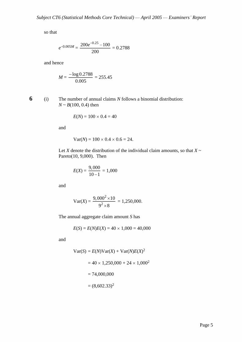
so that
e 0.005M = 0.25200 100
200
e = 0.2788
and hence
M = log 0.2788
0.005 = 255.45
6 (i) The number of annual claims N follows a binomial distribution: N ~ B(100, 0.4) then
E(N) = 100 0.4 = 40
and
Var(N) = 100 0.4 0.6 = 24.
Let X denote the distribution of the individual claim amounts, so that X ~ Pareto(10, 9,000). Then
E(X) = 9,000
10 1 = 1,000
and
Var(X) = 2
2
9,000 10
9 8 = 1,250,000.
The annual aggregate claim amount S has
E(S) = E(N)E(X) = 40 1,000 = 40,000
and
Var(S) = E(N)Var(X) + Var(N)E(X)2
= 40 1,250,000 + 24 1,0002
= 74,000,000
= (8,602.33)2

Subject CT6 (Statistical Methods Core Technical) April 2005
Examiners Report
Page 6
(ii) (a) Since claims can only fall on one day of the year, there is effectively only one day of the year on which ruin can occur, namely 1 August (or strictly shortly thereafter). For a year after 1 August, the insurer will be receiving premiums but paying no claims, and hence solvency will be improving. Hence
(U, t1) = (U, t2) if 7/12 < t1, t2 < 19/12.
(b) We must find (15,000, 1). But ruin will have occurred before time 1 only if it occurs at t = 7/12. Just before the claims occur, the insurers assets will be 7/12 100 600 + 15,000 = 50,000 and ruin will occur if the aggregate claims in the first year exceed this level. Assuming that S is approximately normally distributed, we have
P(Ruin) = P(N(40,000, (8,602.33)2) > 50,000)
=50,000 40,000
(0,1)8,602.33
P N
= 1 (1.162)
= 0.123.
7 (i) Denote:
0 just had a claim 0* 1 claim free year after accident or new customer 1 25% 2 50%
Premiums if no claim Premiums if claim Difference
0 750, 562.50, 375 750, 750, 562.50 375 0* 562.50, 375, 375 750, 750, 562.50 750 1 375, 375, 375 750, 750, 562.50 937.50 2 375, 375, 375 750, 750, 562.50 937.50
So minimum claim in state 0 is 375, in state 0* is 750 and in states 1 and 2 is 937.50.
Subject CT6 (Statistical Methods Core Technical) April 2005
Examiners Report
Page 7
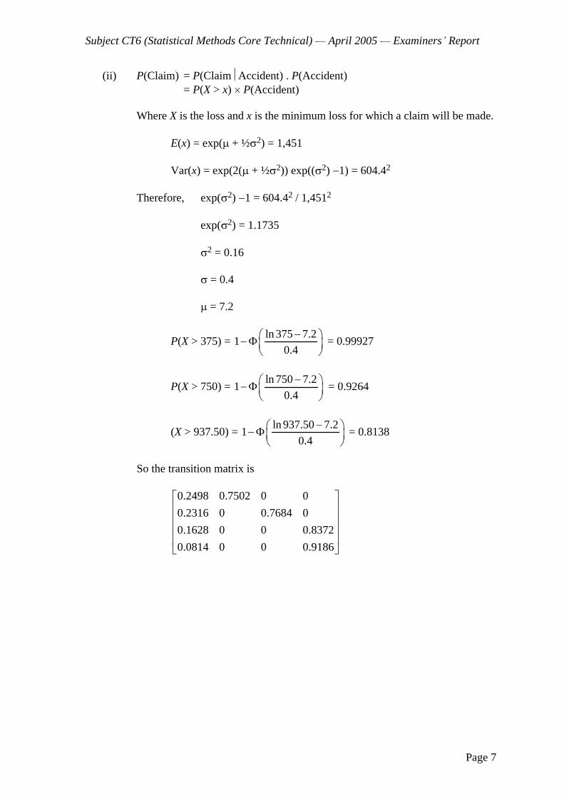
(ii) P(Claim) = P(Claim Accident) . P(Accident) = P(X > x)
P(Accident)
Where X is the loss and x is the minimum loss for which a claim will be made.
E(x) = exp( + ½ 2) = 1,451
Var(x) = exp(2( + ½ 2)) exp(( 2) 1) = 604.42
Therefore, exp( 2) 1 = 604.42 / 1,4512
exp( 2) = 1.1735
2 = 0.16
= 0.4
= 7.2
P(X > 375) = ln 375 7.2
10.4
= 0.99927
P(X > 750) = ln 750 7.2
10.4
= 0.9264
(X > 937.50) = ln 937.50 7.2
10.4
= 0.8138
So the transition matrix is
0.2498 0.7502 0 0
0.2316 0 0.7684 0
0.1628 0 0 0.8372
0.0814 0 0 0.9186
Subject CT6 (Statistical Methods Core Technical) April 2005
Examiners Report
Page 8
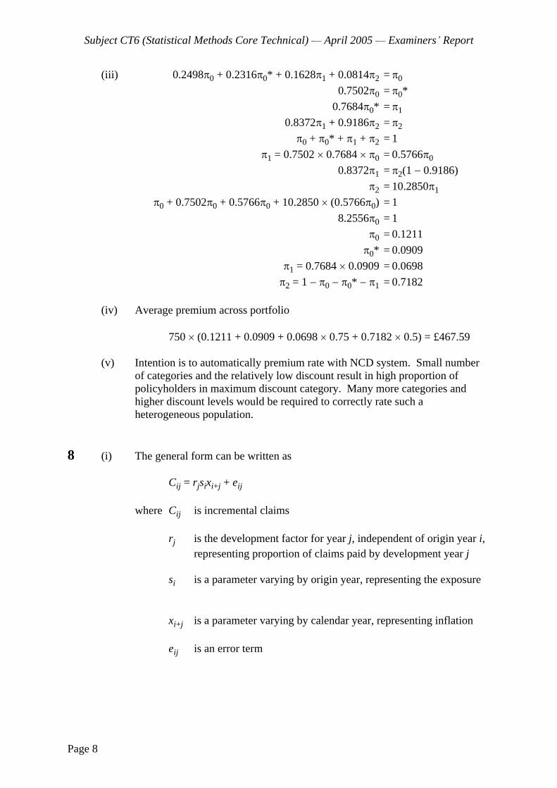
(iii) 0.2498 0 + 0.2316 0* + 0.1628 1 + 0.0814 2 = 0
0.7502 0 = 0*
0.7684 0* = 1
0.8372 1 + 0.9186 2 = 2
0 + 0* + 1 + 2 = 1
1 = 0.7502 0.7684
0 = 0.5766 0
0.8372 1 = 2(1 0.9186)
2 = 10.2850 1
0 + 0.7502 0 + 0.5766 0 + 10.2850 (0.5766 0) = 1
8.2556 0 = 1
0 = 0.1211
0* = 0.0909
1 = 0.7684 0.0909 = 0.0698
2 = 1
0
0* 1 = 0.7182
(iv) Average premium across portfolio
750 (0.1211 + 0.0909 + 0.0698 0.75 + 0.7182 0.5) = £467.59
(v) Intention is to automatically premium rate with NCD system. Small number of categories and the relatively low discount result in high proportion of policyholders in maximum discount category. Many more categories and higher discount levels would be required to correctly rate such a heterogeneous population.
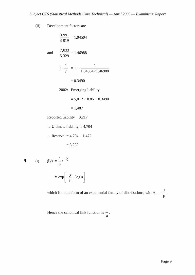
8 (i) The general form can be written as
Cij = rjsixi+j + eij
where Cij is incremental claims
rj is the development factor for year j, independent of origin year i, representing proportion of claims paid by development year j
si is a parameter varying by origin year, representing the exposure
xi+j is a parameter varying by calendar year, representing inflation
eij is an error term
Subject CT6 (Statistical Methods Core Technical) April 2005
Examiners Report
Page 9
(ii) Development factors are
3,991
3,819 = 1.04504
and 7,833
5,329 = 1.46988
11
f
= 1
1
1.04504 1.46988
= 0.3490
2002: Emerging liability
= 5,012 0.85 0.3490
= 1,487
Reported liability 3,217
Ultimate liability is 4,704
Reserve = 4,704 1,472
= 3,232
9 (i) f(y) = 1 y
e
= exp logy
which is in the form of an exponential family of distributions, with = 1
.
Hence the canonical link function is 1
.

Subject CT6 (Statistical Methods Core Technical) April 2005
Examiners Report
Page 10
(ii) (a) The likelihood is 1
( )n
ii
f y = 1
1 yii
n
ii
e
The log-likelihood is
1
= logn
ii
ii
y
Hence c
= 1 1
( ) ( )m n
i ii i m
e y e y
= 1 1
( )m n
i ii i m
m n m e y e y
(b) c
= 1
m
ii
m e y
c
= 0
1
= 0m
ii
m e y
= 1log
m
ii
y
m
c
= 1
( )n
ii m
n m e y
c
= 0
1
( )n
ii m
n m e y = 0
= 1log
n
ii m
y
n m
(c) The deviance is 2( )f c
f = 1
logn
ii
ii
yy
y =
1
logn
ii
y n

Subject CT6 (Statistical Methods Core Technical) April 2005
Examiners Report
Page 11
Hence the deviance is
1 1
1 1 1
1 1
2 log log log1 1
m n
i jn m nj j mi i
im n
i j i mj j
j j m
y yy y
y nm n m
y ym n m
= 1 1 1 1 1
1 12 log log log
n m m n n
i j ji i j i m j m
y n y m y n mm n m
= 1 1
1 1
1 1
2 log log
m n
j jm nj j m
i ii i m
y ym n m
y y
(iii) The deviance residual is sign ( )i i iy y D where the deviance is 1
.n
ii
D
iy
= 14.2
D1 = 11
1
1
12 log 1 log
1
m
i mi
ii
yy y
my
m
= 7
2 log 7 1 log14.214.2
= 0.2
Hence the deviance residual is 0.2

Subject CT6 (Statistical Methods Core Technical) April 2005
Examiners Report
Page 12
10 (i) If, having take a sample from the distribution parameterised by , the posterior distribution of belongs to the same family as the prior distribution then the prior is called a conjugate prior.
(ii) We know that the prior distribution of is ( , s). If X
is the sample taken
from the exponential distribution, then the posterior density satisfies:
f( X)
f(X )f( )
= 1
1 ( )i
n sx
i
s ee
1( )1n
iis xn e
pdf of 1
,n
ii
n s x
This means that the posterior distribution of also follows a Gamma distribution and therefore the Gamma distribution satisfies the definition of a conjugate prior.
(iii) (a) We know that ~ ( , s). So
E(1/ ) = 0
( )fd
= 1
0 ( )
ss ed
= 2
0 ( )
ss ed
= 1 2
01 ( 1)
ss s ed
= 1
s 1
= 1
s
since the final integral is of the pdf of a (
1, s) distribution.

Subject CT6 (Statistical Methods Core Technical) April 2005
Examiners Report
Page 13
(b) Posterior mean is E(1/ ) where 1
~ , .n
ii
n s x The prior
mean is .1
s The previous result implies that the posterior mean is
given by
11
1
n
i
s x
n
= 1
1
1 1
n
i
xs
n n
= 1
11
1 1 1
n
i
xs n
n n n
and 1
1 1
n
n n = 1
(iv) First consider Alan s beliefs. We know from the formula given in the question that
Var(1/ ) = E(1/ )2
1
2
Hence for Alan we have
0.52 = 32
1
2
which means that
2 = 9
0.25 = 36
and hence = 38. Using the result for the posterior mean, we have 1
s = 3
and hence s = 3
37 = 111. So Alan s prior distribution for is (38, 111).
Similarly for Beatrice, we have
Var(1/ ) = E(1/ )2
1
2

Subject CT6 (Statistical Methods Core Technical) April 2005
Examiners Report
Page 14
Hence
12 = 62
1
2
which means that
2 = 36
1 = 36
and hence = 38 again. Using the results for the posterior mean, we have
1
s = 6 and hence s = 6
37 = 222. So Beatrice s prior distribution for is
(38, 222).
We will use the weighted average formula above to calculate the difference in the posterior means. First note that since both Alan and Beatrice have the same we have
ZA = ZB = 1
1n =
37.
37 n
So the difference in posterior means is given by
ZA 3 + (1
ZA)
x
ZB 6 (1
ZB)
x = 3
Z.
So we need to ensure that n is large enough that
3Z < 1
Z < 1/3
37
37 n< 1/3
3737
3
m
3 37 37 < n
n > 74.
END OF EXAMINERS REPORT

Faculty of Actuaries Institute of Actuaries
EXAMINATION
15 September 2005 (am)
Subject CT6 Statistical Methods Core Technical
Time allowed: Three hours
INSTRUCTIONS TO THE CANDIDATE
1. Enter all the candidate and examination details as requested on the front of your answer booklet.
2. You must not start writing your answers in the booklet until instructed to do so by the supervisor.
3. Mark allocations are shown in brackets.
4. Attempt all 10 questions, beginning your answer to each question on a separate sheet.
5. Candidates should show calculations where this is appropriate.
Graph paper is not required for this paper.
AT THE END OF THE EXAMINATION
Hand in BOTH your answer booklet, with any additional sheets firmly attached, and this question paper.
In addition to this paper you should have available the 2002 edition of the Formulae and Tables and your own electronic calculator.
Faculty of Actuaries CT6 S2005 Institute of Actuaries
CT6 S2005 2
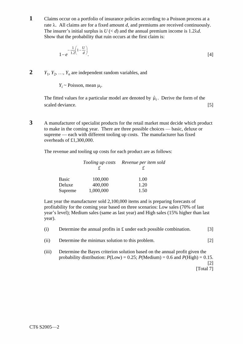
1 Claims occur on a portfolio of insurance policies according to a Poisson process at a rate . All claims are for a fixed amount d, and premiums are received continuously. The insurer s initial surplus is U (< d) and the annual premium income is 1.2 d. Show that the probability that ruin occurs at the first claim is:
11
1.21 .
U
de
[4]
2 Y1, Y2, , Yn are independent random variables, and
Yi ~ Poisson, mean i.
The fitted values for a particular model are denoted by i . Derive the form of the
scaled deviance. [5]
3 A manufacturer of specialist products for the retail market must decide which product to make in the coming year. There are three possible choices basic, deluxe or supreme each with different tooling up costs. The manufacturer has fixed overheads of £1,300,000.
The revenue and tooling up costs for each product are as follows:
Tooling up costs Revenue per item sold £ £
Basic 100,000 1.00 Deluxe 400,000 1.20 Supreme 1,000,000 1.50
Last year the manufacturer sold 2,100,000 items and is preparing forecasts of profitability for the coming year based on three scenarios: Low sales (70% of last year s level); Medium sales (same as last year) and High sales (15% higher than last year).
(i) Determine the annual profits in £ under each possible combination. [3]
(ii) Determine the minimax solution to this problem. [2]
(iii) Determine the Bayes criterion solution based on the annual profit given the probability distribution: P(Low) = 0.25; P(Medium) = 0.6 and P(High) = 0.15.
[2] [Total 7]
CT6 S2005 3 PLEASE TURN OVER
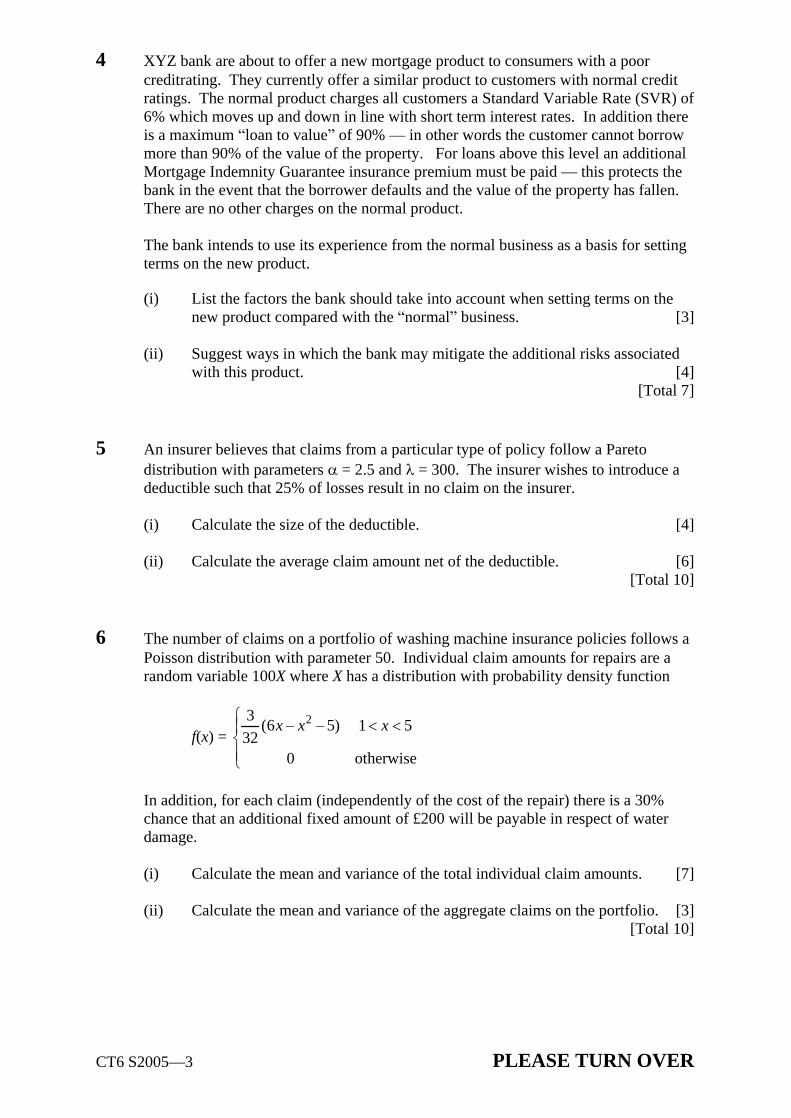
4 XYZ bank are about to offer a new mortgage product to consumers with a poor creditrating. They currently offer a similar product to customers with normal credit ratings. The normal product charges all customers a Standard Variable Rate (SVR) of 6% which moves up and down in line with short term interest rates. In addition there is a maximum loan to value of 90% in other words the customer cannot borrow more than 90% of the value of the property. For loans above this level an additional Mortgage Indemnity Guarantee insurance premium must be paid this protects the bank in the event that the borrower defaults and the value of the property has fallen. There are no other charges on the normal product.
The bank intends to use its experience from the normal business as a basis for setting terms on the new product.
(i) List the factors the bank should take into account when setting terms on the new product compared with the normal business. [3]
(ii) Suggest ways in which the bank may mitigate the additional risks associated with this product. [4]
[Total 7]
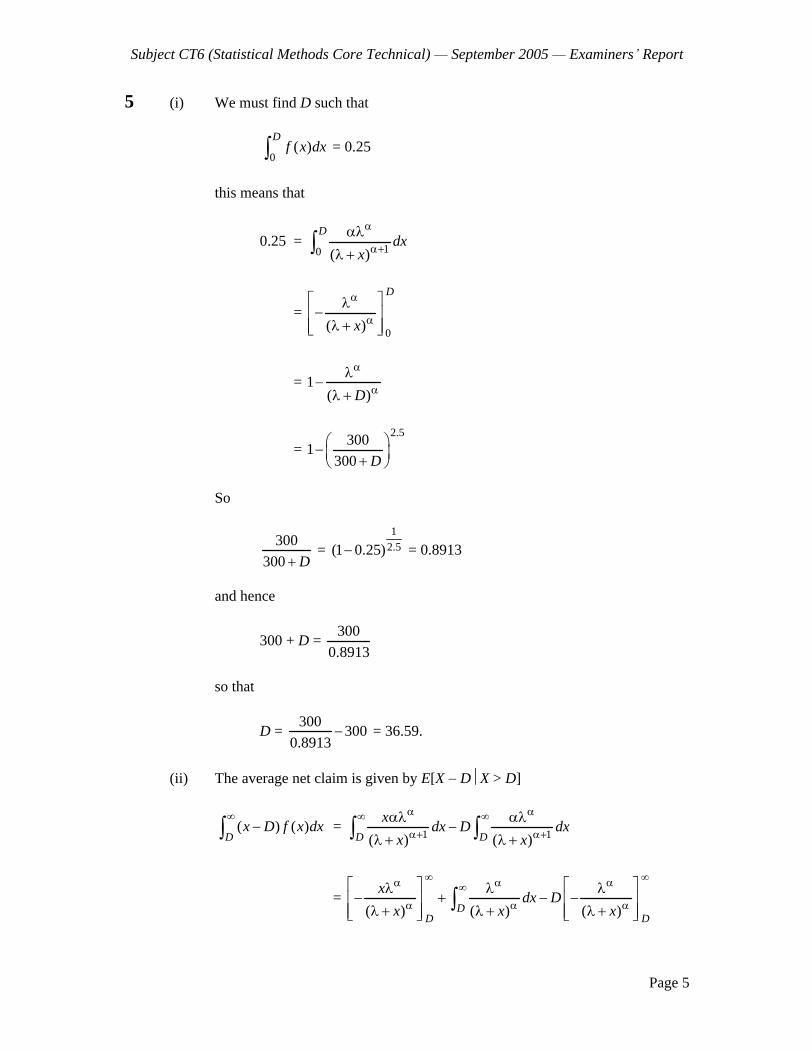
5 An insurer believes that claims from a particular type of policy follow a Pareto distribution with parameters = 2.5 and = 300. The insurer wishes to introduce a deductible such that 25% of losses result in no claim on the insurer.
(i) Calculate the size of the deductible. [4]
(ii) Calculate the average claim amount net of the deductible. [6] [Total 10]
6 The number of claims on a portfolio of washing machine insurance policies follows a Poisson distribution with parameter 50. Individual claim amounts for repairs are a random variable 100X where X has a distribution with probability density function
f(x) = 23
(6 5) 1 532
0 otherwise
x x x
In addition, for each claim (independently of the cost of the repair) there is a 30% chance that an additional fixed amount of £200 will be payable in respect of water damage.
(i) Calculate the mean and variance of the total individual claim amounts. [7]
(ii) Calculate the mean and variance of the aggregate claims on the portfolio. [3] [Total 10]

CT6 S2005 4
7 An insurer operates a simple no claims discount system with 5 levels: 0%, 20%, 40%, 50% and 60%.
The rules for moving between levels are:
An introductory discount of 20% is available to new customers.
If no claims are made during a year the policyholder moves up to the next discount level or remains at the maximum level.
If one or more claims are made during the year, a policyholder at the 50% or 60% discount level moves to the 20% level and a policyholder at 0%, 20% or 40% moves to or remains at the 0% level.
The full annual premium is £600.
When an accident occurs, the distribution of loss is exponential with mean £1,750. A policyholder will only claim if the loss is greater than the extra premiums over the next four years, assuming no further accidents occur.
(i) For each discount level, calculate the smallest cost for which a policyholder will make a claim. [3]
(ii) For each discount level, calculate the probability of a claim being made in the event of an accident occurring. [3]
(iii) Comment on the results of (ii). [2]
(iv) Currently, equal numbers of customers are in each discount level and the probability of a policyholder not having an accident each year is 0.9. Calculate the expected proportions in each discount level next year. [4]
[Total 12]
8 The following time series model is used for the monthly inflation rate (Yt) in a particular country:
Yt = 0.4Yt 1 + 0.2Yt 2 + Zt + 0.025
where {Zt} is a sequence of uncorrelated identically distributed random variables whose distributions are normal with mean zero.
(i) Derive the values of p, d and q, when this model is considered as an ARIMA(p, d, q) model. [3]
(ii) Determine whether {Yt} is a stationary process. [2]
(iii) Assuming an infinite history, calculate the expected value of the rate of inflation over this. [1]

CT6 S2005 5 PLEASE TURN OVER
(iv) Calculate the autocorrelation function of {Yt}. [5]
(v) Explain how the equivalent infinite-order moving average representation of {Yt} may be derived. [2]
[Total 13]
9 The claims paid to date on a motor insurance policy are as follows (Figures in £000s):
Development year Policy Year 0 1 2 3
2001 1,256 945 631 378 2002 1,439 1,072 723 2003 1,543 1,133 2004 1,480
Inflation for the 12 months to the middle of each year was as follows:
2002 2.10% 2003 1.20% 2004 0.80%
Annual premiums written in 2004 were £5,250,000.
Future inflation from mid-2004 is estimated to be 2.5% per annum.
The ultimate loss ratio (based on mid-2004 prices) has been estimated at 75%.
Claims are assumed to be fully run-off at the end of development year 3.
Estimate the outstanding claims arising from policies written in 2004 only (taking explicit account of the inflation statistics in both cases), using:
(i) The chain ladder method. [9]
(ii) The Bornhuetter-Ferguson method. [7] [Total 16]

CT6 S2005 6
10 The total amounts claimed each year from a portfolio of insurance policies over n years were 1 2, , , nx x x . The insurer believes that annual claims have a normal
distribution with mean and variance 21 , where is unknown. The prior distribution
of is assumed to be normal with mean and variance 22 .
(i) Derive the posterior distribution of . [4]
(ii) Using the answer in (a), write down the Bayesian point estimate of under quadratic loss. [2]
(iii) Show that the answer in (b) can be expressed in the form of a credibility estimate and derive the credibility factor. [2]
The claims experience over five years for two companies was as follows:
Year 1 2 3 4 5
Company A Amount 421 417 438 456 463 Company B Amount 343 335 356 366 380
(iv) Determine the Bayes credibility estimate of the premiums the insurer should charge for each company based on the modelling assumptions of part (i), a profit loading of 25% and the following parameters:
Company A Company B
400 300 21
500 350 22
800 600
[6]
(v) Comment on the effect on the result of increasing 21 and 2
2 . [2]
[Total 16]
END OF PAPER
Faculty of Actuaries Institute of Actuaries
EXAMINATION
September 2005
Subject CT6 Statistical Methods Core Technical
EXAMINERS REPORT
Faculty of Actuaries Institute of Actuaries
Subject CT6 (Statistical Methods Core Technical) September 2005
Examiners Report
Page 2
EXAMINERS COMMENTS
Comments on solutions presented to individual questions for this September 2005 paper are given below.
Q1 The general standard of answers was poor. Very few candidates correctly derived the condition for ruin to occur in terms of time until the first claim.
Q2 Reasonably well answered.
Q3 Well answered by the majority of candidates.
Q4 Very few candidates generated enough different points to score high marks on this question.
Q5 Most candidates were able to answer part (i). Answers to part (ii) were more varied, with many candidates struggling with the necessary integration, or evaluating the wrong integral.
Q6 Reasonably well answered, but a large number of candidates failed to cope with the possible additional fixed claim amounts. A common error was to treat the separate elements as entirely independent which is incorrect since the fixed claim can only occur when a variable claim has already been made.
Q7 Answers were generally of a high standard. However, a surprisingly large number of candidates ignored the instruction in part (iv) of the question and instead derived the proportions in each state in a stationary population.
Q8 In general this was reasonably well answered, although many candidates failed to give any justification for their classification in part (i). In part (iv) a number of candidates claimed that the autocorrelation function was zero for k greater than 2.
Q9 The inflation adjustment needed to past claims data produced a number of common alternative approaches credit was given for these providing they were sensible, consistent and clearly explained. Most candidates were able to derive the necessary development factors. However, a large number of candidates failed to adjust the outstanding claims for future inflation (ie the answer was given in 2004 prices) and so failed to obtain full marks. Many candidates did not show any working for the calculations in part (ii) making it difficult to give any credit for partially correct solutions.
Q10 Many candidates simply wrote down the result in part (i) (which is given in the tables) rather than deriving it as instructed. The rest of the question was very well answered in general.

Subject CT6 (Statistical Methods Core Technical)
September 2005
Examiners Report
Page 3
1 Ruin will occur if the time of the first claim t is such that
U + 1.2 dt < d
i.e. if
t < .1.2
d U
d
The time until the first claim follows an exponential distribution with parameter . So the probability of ruin is given by
1.20
d Uxd e dx
= 1.20
d Ux de
= 1.21
d U
de
=
11
1.21 .
U
de
2 The deviance is 2(lf
lc), where lf and lc are the log-likelihoods of the full and current model, respectively.
f(y) = !
ye
y
l = 1
log log !n
i i i ii
y y
lf = 1
log log !n
i i i ii
y y y y
lc = 1
log log !n
i i i ii
y y
Hence the deviance is
1 1
2 log ( )n n
ii i i
ii i
yy y

Subject CT6 (Statistical Methods Core Technical) September 2005
Examiners Report
Page 4
3 (i) Revenue (£)
Low Medium High
Basic 1,470,000 2,100,000 2,415,000 Deluxe 1,764,000 2,520,000 2,898,000 Supreme 2,205,000 3,150,000 3,622,500
Costs (£)
Low Medium High
Basic 1,400,000 1,400,000 1,400,000 Deluxe 1,700,000 1,700,000 1,700,000 Supreme 2,300,000 2,300,000 2,300,000
Profit (£)
Low Medium High Min Max Expected Profit
Basic 70,000 700,000 1,015,000 70,000
1,015,000 589,750
Deluxe 64,000 820,000 1,198,000 64,000
1,198,000 687,700
Supreme
95,000 850,000 1,322,500 95,000
1,322,500 684,625
(ii) Minimax: Decision is Basic .
(iii) Highest expected profit. Decision is Deluxe .
4 (i) Higher risk of default. Cost of MIG insurance. Other insurers. Cost of underwriting. Profitability of normal product. Adjust for underlying economic conditions. Exceptional defaults.
(ii) Higher SVR. Lower LTV. Higher MIG. Penalty Payments. Increase charges. Compulsory insurance. Maximum loan amount. Charges/SVR variable according to wish.
Other sensible suggestions were given credit.
Subject CT6 (Statistical Methods Core Technical) September 2005
Examiners Report
Page 5
5 (i) We must find D such that
0( )
Df x dx = 0.25
this means that
0.25 = 10 ( )
Ddx
x
= 0
( )
D
x
= 1( )D
= 2.5
3001
300 D
So
300
300 D =
12.5(1 0.25) = 0.8913
and hence
300 + D = 300
0.8913
so that
D = 300
3000.8913
= 36.59.
(ii) The average net claim is given by E[X
D X > D]
( ) ( )D
x D f x dx
= 1 1( ) ( )D D
xdx D dx
x x
= ( ) ( ) ( )D
D D
xdx D
x x x

Subject CT6 (Statistical Methods Core Technical) September 2005
Examiners Report
Page 6
= 1
0 0( ) ( 1)( ) ( )
D
D D
D x D
=
1( 1)( )D
= 2.5
1.5
300
1.5 (300 36.59)
= 168.29.
Hence E[X
D X > D] = 168.29
0.75 = 224.39
6 We first calculate E(100X) and Var(100X). Taking the expectation first, we have
E(100X) = 100E(X)
= 5 2 3
1
3100 6 5
32x x xdx
=
54 23
1
300 52
32 4 2
x xx
= 300
(31.25 0.75)32
= 300.
Now for the variance
E((100X)2) = 1002
E(X2)
= 52 3 4 2
1
3100 6 5
32x x x dx
=
54 5 3
1
30,000 6 5
32 4 5 3
x x x
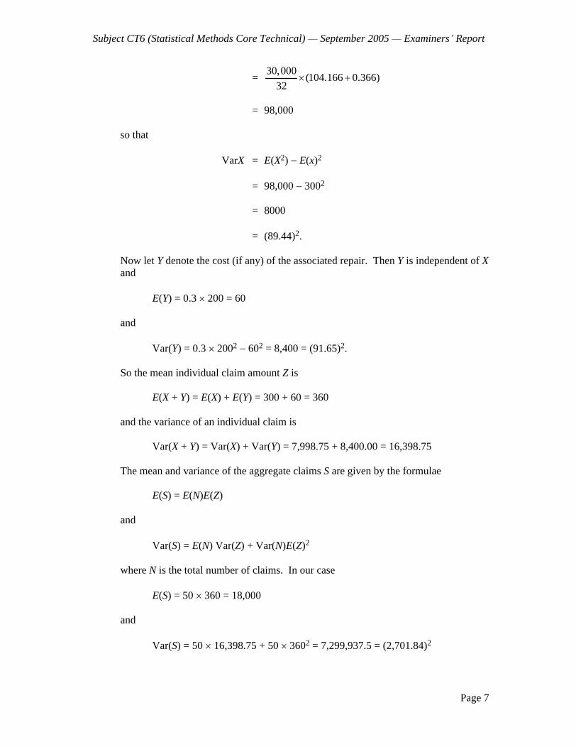
Subject CT6 (Statistical Methods Core Technical) September 2005
Examiners Report
Page 7
= 30,000
(104.166 0.366)32
= 98,000
so that
VarX = E(X2)
E(x)2
= 98,000 3002
= 8000
= (89.44)2.
Now let Y denote the cost (if any) of the associated repair. Then Y is independent of X and
E(Y) = 0.3 200 = 60
and
Var(Y) = 0.3 2002 602 = 8,400 = (91.65)2.
So the mean individual claim amount Z is
E(X + Y) = E(X) + E(Y) = 300 + 60 = 360
and the variance of an individual claim is
Var(X + Y) = Var(X) + Var(Y) = 7,998.75 + 8,400.00 = 16,398.75
The mean and variance of the aggregate claims S are given by the formulae
E(S) = E(N)E(Z)
and
Var(S) = E(N) Var(Z) + Var(N)E(Z)2
where N is the total number of claims. In our case
E(S) = 50 360 = 18,000
and
Var(S) = 50 16,398.75 + 50 3602 = 7,299,937.5 = (2,701.84)2

Subject CT6 (Statistical Methods Core Technical) September 2005
Examiners Report
Page 8
7 (i) Discount level Premiums if no claim Premiums if claim Difference
0% 480, 360, 300, 240 600, 480, 360, 300 360 20% 360, 300, 240, 240 600, 480, 360, 300 600 40% 300, 240, 240, 240 600, 480, 360, 300 720
50%/60% 240, 240, 240, 240 480, 360, 300, 240 420
(ii)
0% P(Cost > 360) = exp( 360/1,750) = 0.814 20% P(Cost > 600) = exp( 600/1,750) = 0.710 40% P(Cost > 720) = exp( 720/1,750) = 0.663 50%/60% P(Cost > 420) = exp( 420/1,750) = 0.787
(iii) The amount for which the 50%/60% discount drivers will claim is much lower than the 20% and 40% categories. It seems illogical for this to be the case as this leads to a higher probability of a claim in the event of an accident. Suggest that structure is altered to make claims for these categories less likely.
(iv) The transition matrix is
0.0814 0.9186 0 0 0
0.0710 0 0.9290 0 0
0.0663 0 0 0.9337 0
0 0.0787 0 0 0.9213
0 0.0787 0 0 0.9213
This year the proportions at each level are
(0.2, 0.2, 0.2, 0.2, 0.2)
Next year, the expected proportions are
0.2 (0.0814 + 0.0710 + 0.0663) = 0.04374 0.2 (0.9186 + 0.0787 + 0.0787) = 0.2152 0.2 0.9290 = 0.1858 0.2 0.9337 = 0.18674 0.2 (0.9213 + 0.9213) = 0.36852

Subject CT6 (Statistical Methods Core Technical) September 2005
Examiners Report
Page 9
8 (i) (1 0.4B 0.2B2) Yt = Zt + 0.025
Characteristic equation
1 0.4z 0.2z2 = 0
has no root at z = 1, so d = 0.
No functional dependence on Zt 1, Zt 2, etc., so q = 0.
Hence this is an ARIMA(2, 0, 0).
(ii) Roots of characteristic equation are 1 6 , which are outside ( 1, +1), so {Yt} is stationary.
(iii) Mean is stationary over time
(1 0.4 0.2)E[Yt] = 0.025
E[Yt] = 0.025
0.4 = 0.0625.
(iv) Yt 0.0625 = 0.4(Yt 1 0.0625) + 0.2(Yt 2 0.0625) + Zt
k = E[(Yt 0.0625)(Yt k 0.0625)] = 0.4 k 1 + 0.2 k 2
Put k = 1, and note that 0 = 1 and 1 = 1
1 = 0.4 + 0.2 1
1 = 0.4
0.8 = 0.5
2 = 0.4 1 + 0.2 = 0.4
3 = 0.4 2 + 0.2 1 = 0.26
and so on.
(v) (1 0.4B 0.2B2)(Yt 0.0625) = zt
Yt 0.0625 = (1 0.4B 0.2B2) 1Zt
So we need to invert (1 0.4B 0.2B2) and multiply by Zt to obtain the equivalent moving average process.

Subject CT6 (Statistical Methods Core Technical) September 2005
Examiners Report
Page 10
9 (Figures in £000s)
Inflation factors for each development year AY 0
1
2
3
2001 1.02499
1.00390
0.99200
1.00000
2002 1.00390
0.99200
1.00000
2003 0.99200
1.00000
2004 1.00000
Other inflation adjustments were given credit providing they were sensible, consistent and some explanation was given.
Inflation adjusted claim payments in mid 2004 prices
AY 0
1
2
3
2001 1,287.39
948.69
625.95
378
2002 1,444.61
1,063.42
723
2003 1,530.66
1,133
2004 1,480
Inflation adjusted cumulative claim payments in mid 2004 prices
AY 0
1
2
3
2001 1,287.39
2,236.08
2,862.03
3,240.03
2002 1,444.61
2,508.03
3,231.03
2003 1,530.66
2,663.66
2004 1,480
Column sum
7,407.77
6,093.06
3,240.03
Column sum minus last entry 4,262.66
4,744.11
2,862.03
Development factor 1.73783
1.28434
1.13207
(i)
Outstanding amounts arising from 2004 policies
Accumulated
1,480.0
2,572.0
3,303.3
3,739.6
Disaccumulated
1,092.0
731.3
436.3
Inflation
1.025
1.050625
1.076891
Inflation adj by year
1,119.3
768.3
469.8
Total
2,357.4
For example, 2,572.0 = 1,480 1.7378
Subject CT6 (Statistical Methods Core Technical) September 2005
Examiners Report
Page 11
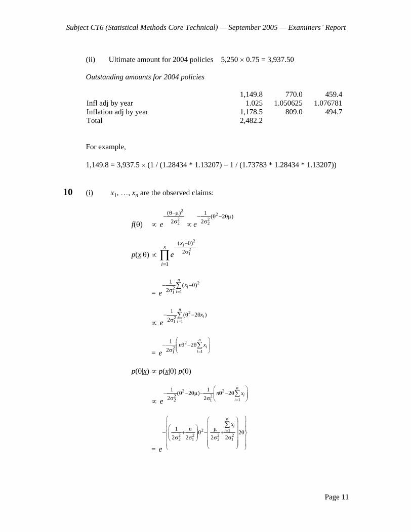
(ii) Ultimate amount for 2004 policies 5,250 0.75 = 3,937.50
Outstanding amounts for 2004 policies
1,149.8
770.0
459.4
Infl adj by year
1.025
1.050625
1.076781
Inflation adj by year
1,178.5
809.0
494.7
Total
2,482.2
For example,
1,149.8 = 3,937.5 (1 / (1.28434 * 1.13207) 1 / (1.73783 * 1.28434 * 1.13207))
10 (i) x1, , xn are the observed claims:
f( )
22
2 22 2
( ) 1( 2 )
2 2e e
p(x )
21
21
( )
2
1
xx
i
e
=
22
11
1( )
2
n
ii
x
e
22
11
1( 2 )
2
n
ii
x
e
=
22
11
12
2
n
ii
n x
e
p( x)
p(x ) p( )
2 22 2
12 1
1 1( 2 ) 2
2 2
n
ii
n x
e
=
2 12 2 2 22 1 2 1
12
2 2 2 2
n
ii
xn
e

Subject CT6 (Statistical Methods Core Technical) September 2005
Examiners Report
Page 12
=
2 21 22 2
2 11 22 2 2 21 2 1 2
22 2
n
ii
xn
e
2
222 2 2
1 2 1 12 2 2 2 2 21 2 1 2 1 22
n
ii
xn
n n
e
x ~
2 21 2 2 2
1 1 22 2 2 21 2 1 2
,
n
ii
x
Nn n
(ii) Point estimator under quadratic loss is the posterior mean:
E( x) = 2 21 2
2 2 2 211 2 1 2
n
ii
xn n
(iii) E( x) = (1
Z) + Z 1
n
ii
x
n
which is in the form of a credibility estimate, and
Z = 22
2 21 2
n
n
is the credibility factor.
(iv) Company A Company B
n 5 5
21
500 350
22
800 600
Z = 22
22 12 n
0.8889 0.8955
x
439 356
400 300
Subject CT6 (Statistical Methods Core Technical) September 2005
Examiners Report
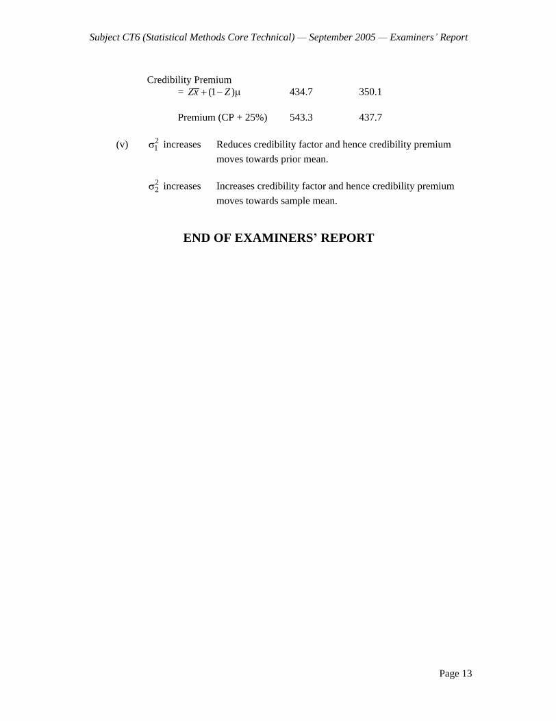
Page 13
Credibility Premium = (1 )Zx Z
434.7 350.1
Premium (CP + 25%) 543.3 437.7
(v) 21 increases Reduces credibility factor and hence credibility premium
moves towards prior mean.
22 increases Increases credibility factor and hence credibility premium
moves towards sample mean.
END OF EXAMINERS REPORT

Faculty of Actuaries Institute of Actuaries
EXAMINATION
28 March 2006 (am)
Subject CT6 Statistical Methods Core Technical
Time allowed: Three hours
INSTRUCTIONS TO THE CANDIDATE
1. Enter all the candidate and examination details as requested on the front of your answer booklet.
2. You must not start writing your answers in the booklet until instructed to do so by the supervisor.
3. Mark allocations are shown in brackets.
4. Attempt all 10 questions, beginning your answer to each question on a separate sheet.
5. Candidates should show calculations where this is appropriate.
Graph paper is not required for this paper.
AT THE END OF THE EXAMINATION
Hand in BOTH your answer booklet, with any additional sheets firmly attached, and this question paper.
In addition to this paper you should have available the 2002 edition of the Formulae and Tables and your own electronic calculator.
Faculty of Actuaries CT6 A2006 Institute of Actuaries

CT6 A2006 2
1 List the main perils typically insured against under a household buildings policy. [3]
2 A No Claims Discount (NCD) system has 3 levels of discount
Level 0 no discount Level 1 discount = p Level 2 discount = 2p
where 0 < p < 0.5.
The probability of a policyholder NOT making a claim each year is 0.9.
In the event of a claim, the policyholder moves to, or remains at level 0. Otherwise, the policyholder moves to the next higher level (or remains at level 2).
The premium paid in level 0 is £1,000.
Derive an expression in terms of p for the average premium paid by a policyholder once the steady state has been reached. [6]
3 Based on the proposal form, an applicant for life insurance is classified as a standard life (1), an impaired life (2) or uninsurable (3). The proposal form is not a perfect classifier and may place the applicant into the wrong category.
The decision to place the applicant in state i is denoted by di, and the correct state for
the applicant is i.
The loss function for this decision is shown below:
d1 d2 d3
1 0 5 8
2 12 0 3
3 20 15 0
(i) Determine the minimax solution when assigning an applicant to a category. [1]
(ii) Based on the application form, the correct category for a new applicant appears to be as an impaired life. However, of applicants which appear to be impaired lives, 15% are in fact standard lives and 25% are uninsurable. Determine the Bayes solution for this applicant. [4]
[Total 5]

CT6 A2006 3 PLEASE TURN OVER
4 (i) Derive the autocovariance and autocorrelation functions of the AR(1) process
Xt = Xt 1 + et
where < 1 and the et form a white noise process. [4]
(ii) The time series Zt is believed to follow a ARIMA(1, d, 0) process for some
value of d. The time series ( )ktZ is obtained by differencing k times and the
sample autocorrelations, {ri : i = 1, , 10}, are shown in the table below for various values of k.
k = 0 k = 1 k = 2 k = 3 k = 4 k = 5
r1 100% 100% 83% 3% 45% 64% r2 100% 100% 66% 12% 5% 13% r3 100% 100% 54% 11% 4% 3% r4 100% 99% 45% 1% 6% 4% r5 100% 99% 37% 3% 4% 5% r6 100% 99% 30% 12% 12% 12% r7 99% 98% 27% 3% 7% 9% r8 99% 98% 24% 3% 0% 4% r9 99% 97% 19% 3% 5% 6% r10 99% 97% 13% 7% 5% 4%
Suggest, with reasons, appropriate values for d and the parameter in the underlying AR(1) process. [4]
[Total 8]
5 (i) Let n be an integer and suppose that X1, X2, , Xn are independent random
variables each having an exponential distribution with parameter . Show that Z = X1 + + Xn has a Gamma distribution with parameters n and . [2]
(ii) By using this result, generate a random sample from a Gamma distribution with mean 30 and variance 300 using the 5 digit pseudo-random numbers.
63293 43937 08513 [5] [Total 7]

CT6 A2006 4
6 An insurance company has a set of n risks (i = 1, 2, , n) for which it has recorded the number of claims per month, Yij, for m months (j = 1, 2, , m).
It is assumed that the number of claims for each risk, for each month, are independent Poisson random variables with
E[Yij] = ij .
These random variables are modelled using a generalised linear model, with
log ij = i (i = 1, 2, , n)
(i) Derive the maximum likelihood estimator of i . [4]
(ii) Show that the deviance for this model is
1 1
2 log ( )n m
ijij ij i
ii j
yy y y
y
where 1
1=
m
i ijj
y ym
. [3]
(iii) A company has data for each month over a 2 year period. For one risk, the average number of claims per month was 17.45. In the most recent month for this risk, there were 9 claims. Calculate the contribution that this observation makes to the deviance. [3]
[Total 10]
7 (i) Let N be a random variable representing the number of claims arising from a portfolio of insurance policies. Let Xi denote the size of the ith claim and suppose that X1, X2, are independent identically distributed random variables, all having the same distribution as X. The claim sizes are independent of the number of claims. Let S = X1 + X2 + + XN denote the total claim size. Show that
MS(t) = MN(logMX(t)). [3]
(ii) Suppose that N has a Type 2 negative binomial distribution with parameters k > 0 and 0 < p < 1. That is
P(N = x) = ( )
( 1) ( )k xk x
p qx k
x = 0, 1, 2,
Suppose that X has an exponential distribution with mean 1/ . Derive an expression for Ms(t). [2]
CT6 A2006 5 PLEASE TURN OVER
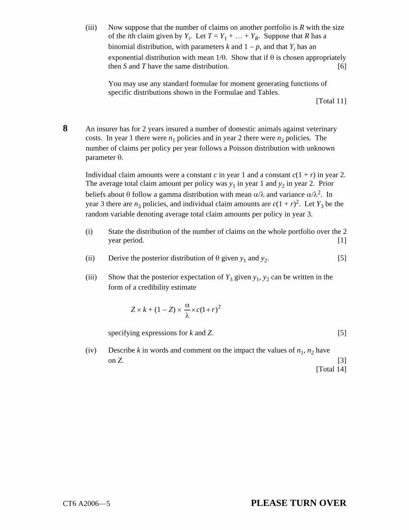
(iii) Now suppose that the number of claims on another portfolio is R with the size of the ith claim given by Yi. Let T = Y1 + + YR. Suppose that R has a
binomial distribution, with parameters k and 1
p, and that Yi has an
exponential distribution with mean 1/ . Show that if
is chosen appropriately
then S and T have the same distribution. [6]
You may use any standard formulae for moment generating functions of specific distributions shown in the Formulae and Tables.
[Total 11]
8 An insurer has for 2 years insured a number of domestic animals against veterinary costs. In year 1 there were n1 policies and in year 2 there were n2 policies. The number of claims per policy per year follows a Poisson distribution with unknown parameter .
Individual claim amounts were a constant c in year 1 and a constant c(1 + r) in year 2. The average total claim amount per policy was y1 in year 1 and y2 in year 2. Prior
beliefs about follow a gamma distribution with mean / and variance / 2. In year 3 there are n3 policies, and individual claim amounts are c(1 + r)2. Let Y3 be the random variable denoting average total claim amounts per policy in year 3.
(i) State the distribution of the number of claims on the whole portfolio over the 2 year period. [1]
(ii) Derive the posterior distribution of given y1 and y2. [5]
(iii) Show that the posterior expectation of Y3 given y1, y2 can be written in the form of a credibility estimate
Z
k + (1
Z)
2(1 )c r
specifying expressions for k and Z. [5]
(iv) Describe k in words and comment on the impact the values of n1, n2 have on Z. [3]
[Total 14]

CT6 A2006 6
9 (i) The general form of a run-off triangle can be expressed as:
Accident Year Development Year
0 1 2 3 4 5
0 C0,0 C0,1 C0,2 C0,3 C0,4 C0,5
1 C1,0 C1,1 C1,2 C1,3 C1,4
2 C2,0 C2,1 C2,2 C2,3
3 C3,0 C3,1 C3,2
4 C4,0 C4,1
5 C5,0
Define a model for each entry, Cij, in general terms and explain each element of the formula. [3]
(ii) The run-off triangles given below relate to a portfolio of motorcycle insurance policies.
The cost of claims paid during each year is given in the table below:
(Figures in £000s)
Accident Year Development Year
0 1 2 3
2002 2,905 535 199 56 2003 3,315 578 159 2004 3,814 693 2005 4,723
The corresponding number of settled claims is as follows:
Accident Year Development Year
0 1 2 3
2002 430 51 24 7 2003 465 58 24 2004 501 59 2005 539
Calculate the outstanding claims reserve for this portfolio using the average cost per claim method with grossing-up factors, and state the assumptions underlying your result. [9]
(iii) Compare the results from the analysis in (ii) with those obtained from the basic chain ladder method. [5]
[Total 17]
CT6 A2006 7
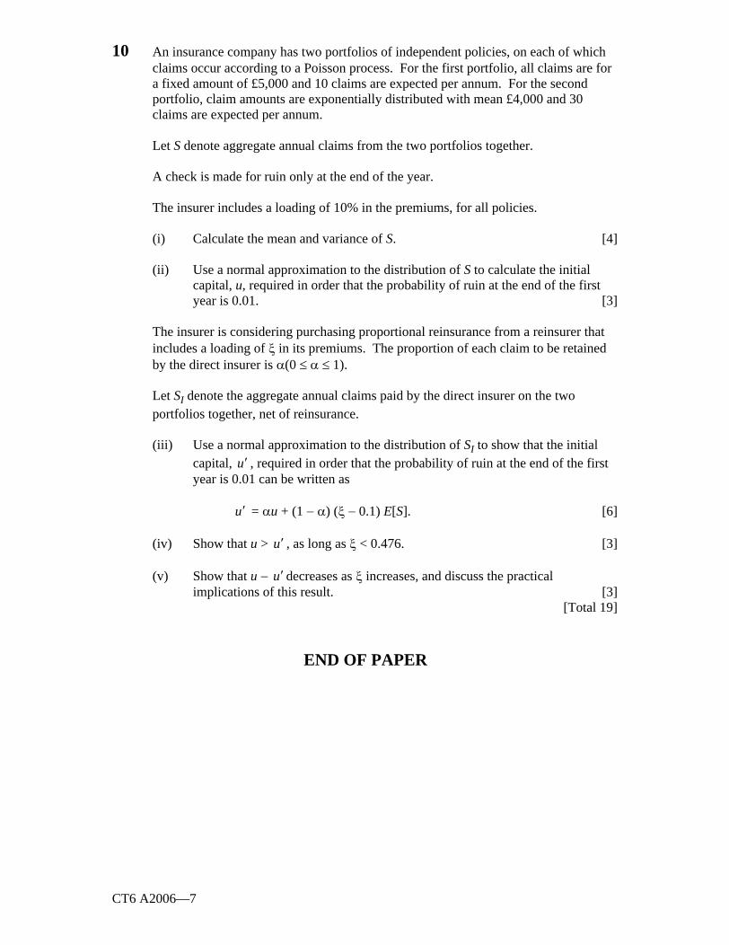
10 An insurance company has two portfolios of independent policies, on each of which claims occur according to a Poisson process. For the first portfolio, all claims are for a fixed amount of £5,000 and 10 claims are expected per annum. For the second portfolio, claim amounts are exponentially distributed with mean £4,000 and 30 claims are expected per annum.
Let S denote aggregate annual claims from the two portfolios together.
A check is made for ruin only at the end of the year.
The insurer includes a loading of 10% in the premiums, for all policies.
(i) Calculate the mean and variance of S. [4]
(ii) Use a normal approximation to the distribution of S to calculate the initial capital, u, required in order that the probability of ruin at the end of the first year is 0.01. [3]
The insurer is considering purchasing proportional reinsurance from a reinsurer that includes a loading of in its premiums. The proportion of each claim to be retained by the direct insurer is (0
1).
Let SI denote the aggregate annual claims paid by the direct insurer on the two portfolios together, net of reinsurance.
(iii) Use a normal approximation to the distribution of SI to show that the initial capital, u , required in order that the probability of ruin at the end of the first year is 0.01 can be written as
u = u + (1
) (
0.1) E[S]. [6]
(iv) Show that u > u , as long as < 0.476. [3]
(v) Show that u
u decreases as increases, and discuss the practical implications of this result. [3]
[Total 19]
END OF PAPER
Faculty of Actuaries Institute of Actuaries
EXAMINATION
April 2006
Subject CT6 Statistical Methods Core Technical
EXAMINERS REPORT
Introduction
The attached subject report has been written by the Principal Examiner with the aim of helping candidates. The questions and comments are based around Core Reading as the interpretation of the syllabus to which the examiners are working. They have however given credit for any alternative approach or interpretation which they consider to be reasonable.
M Flaherty Chairman of the Board of Examiners
June 2006
Comments
Individual comments are shown after each question.
Faculty of Actuaries Institute of Actuaries

Subject CT6 (Statistical Methods Core Technical) April 2006
Examiners Report
Page 2
1 Fire Flood Storm Theft Explosions Lightning Damage caused by measures taken to put out a fire.
Comments on question 1: This straightforward bookwork question was poorly done with relatively few candidates scoring full marks. Credit was given for any other reasonable suggestion not included on the list above.
2 The transition matrix is
0.1 0.9 0
0.1 0 0.9
0.1 0 0.9
0.1 ( 0 + 1 + 2) = 0
0 = 0.1
0.9 0 = 1
1 = 0.09
2 = 0.81
Average premium paid is
[0.1 + 0.09(1
p) + 0.81(1 2p)] 1,000
= [1 0.09p 1.62p] 1,000 p] 1,000
Comments on question 2: Most candidates obtained full marks. A few incorrectly identified the transition matrix or failed to solve the simultaneous equations.
Subject CT6 (Statistical Methods Core Technical) April 2006
Examiners Report
Page 3
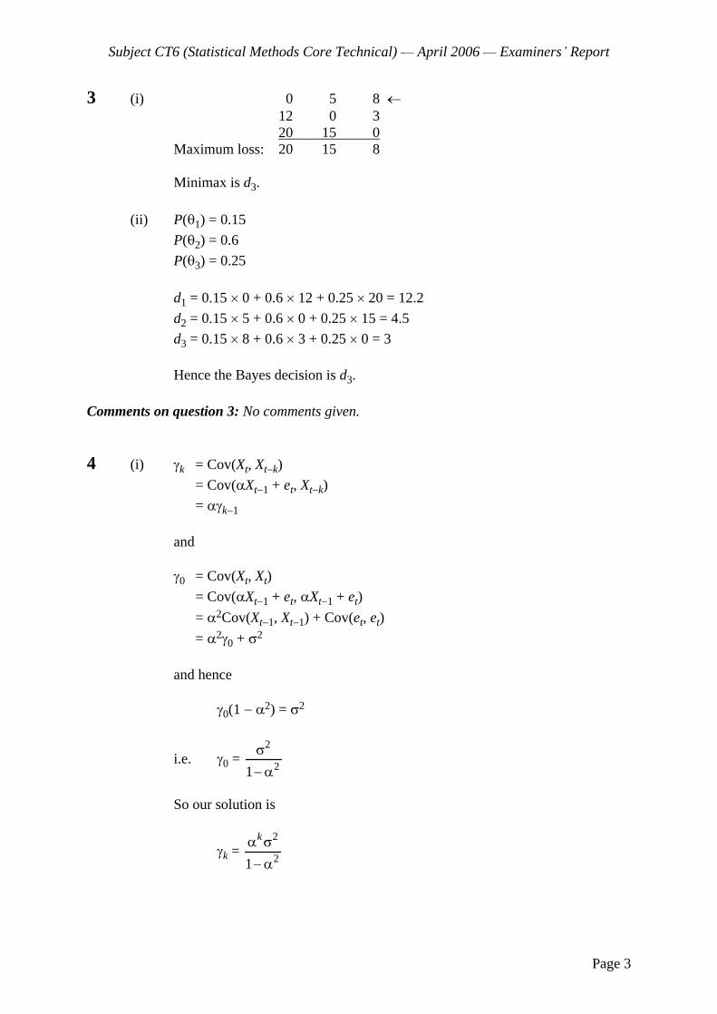
3 (i) 0 5 8
12 0 3 20 15 0
Maximum loss: 20 15 8
Minimax is d3.
(ii) P( 1) = 0.15
P( 2) = 0.6
P( 3) = 0.25
d1 = 0.15 0 + 0.6 12 + 0.25 20 = 12.2
d2 = 0.15 5 + 0.6 0 + 0.25 15 = 4.5
d3 = 0.15 8 + 0.6 3 + 0.25 0 = 3
Hence the Bayes decision is d3.
Comments on question 3: No comments given.
4 (i) k = Cov(Xt, Xt k)
= Cov( Xt 1 + et, Xt k)
= k 1
and
0 = Cov(Xt, Xt)
= Cov( Xt 1 + et, Xt 1 + et)
= 2Cov(Xt 1, Xt 1) + Cov(et, et)
= 20 + 2
and hence
0(1
2) = 2
i.e. 0 = 2
21
So our solution is
k = 2
21
k

Subject CT6 (Statistical Methods Core Technical) April 2006
Examiners Report
Page 4
The autocorrelation function is given by
k = 0
k = k
(ii) The autocorrelation should decay exponentially as i increases. Looking at the table this behaviour occurs after differencing 2 times, suggesting the value of d = 2.
We know that the ratio of successive r s should be . We can form these ratios as follows:
r2/r1 80% r3/r2 82% r4/r3 83% r5/r4 82% r6/r5 81% r7/r6 90% r8/r7 89% r9/r8 79% r10/r9 68%
Average 81.6%
Alternatively we can take the ith root of the ith autocorrelation:
i ith root
1 83% 2 81% 3 81% 4 82% 5 82% 6 82% 7 83% 8 84% 9 83% 10 82%
Average 82%
Both approaches suggest the value of alpha is around 82%.
Full credit should be given to any reasonable approach.
Comments on question 4: This question was generally done poorly. Although most candidates made a reasonable attempt at (i), very few correctly identified appropriate values or sensible reasons in (ii).

Subject CT6 (Statistical Methods Core Technical) April 2006
Examiners Report
Page 5
5 (i) Each Xi has moment generating function ( )iXM t = .
t Hence
MZ(t) = 1 ... ( )
nX XM t = ( )i
nXM t =
n
t
which is the moment generating function of a gamma distribution with parameters n and and hence Z has this distribution.
(ii) = 30, 2
= 300
= 3 and = 0.1
The random sample can be generated by producing three independent samples from an Exponential distribution with parameter 0.1 and adding them together. To do this, we need to solve
FX(x) = 1 - e-0.1x = u
where u is a pseudo-random number from a U(0, 1) distribution.
Solving, we have x = log(1 )
0.1
u
So using our pseudo-random numbers to give the exponential samples we have:
u = 0.63292 x = 10.022 u = 0.43937 x = 5.787 u = 0.08513 x = 0.890
and the sample from the gamma distribution is
10.022 + 5.787 + 0.890 = 16.699.
Comments on question 5: Part (i) was well answered but most candidates failed to generate the required random sample in part (ii).
Subject CT6 (Statistical Methods Core Technical) April 2006
Examiners Report
Page 6
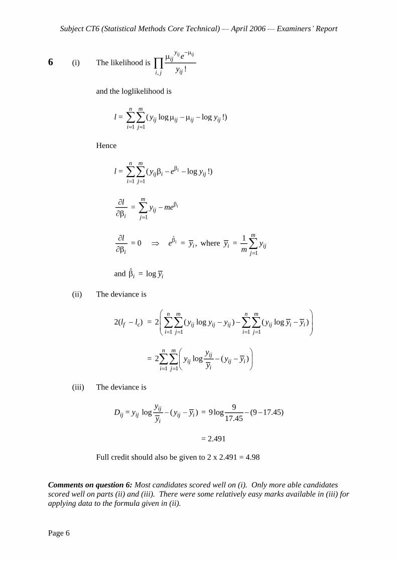
6 (i) The likelihood is , !
ij ijyij
iji j
e
y
and the loglikelihood is
l = 1 1
( log log !)n m
ij ij ij iji j
y y
Hence
l = 1 1
( log !)i
n m
ij i iji j
y e y
i
l =
1
i
m
ijj
y me
i
l = 0 ie = ,iy where iy =
1
1 m
ijj
ym
and i = log iy
(ii) The deviance is
2(lf lc) = 1 1 1 1
2 ( log ) ( log )n m n m
ij ij ij ij i ii j i j
y y y y y y
= 1 1
2 log ( )n m
ijij ij i
ii j
yy y y
y
(iii) The deviance is
Dij = yij log ( )ijij i
i
yy y
y
= 9
9log (9 17.45)17.45
= 2.491
Full credit should also be given to 2 x 2.491 = 4.98
Comments on question 6: Most candidates scored well on (i). Only more able candidates scored well on parts (ii) and (iii). There were some relatively easy marks available in (iii) for applying data to the formula given in (ii).
Subject CT6 (Statistical Methods Core Technical) April 2006
Examiners Report
Page 7
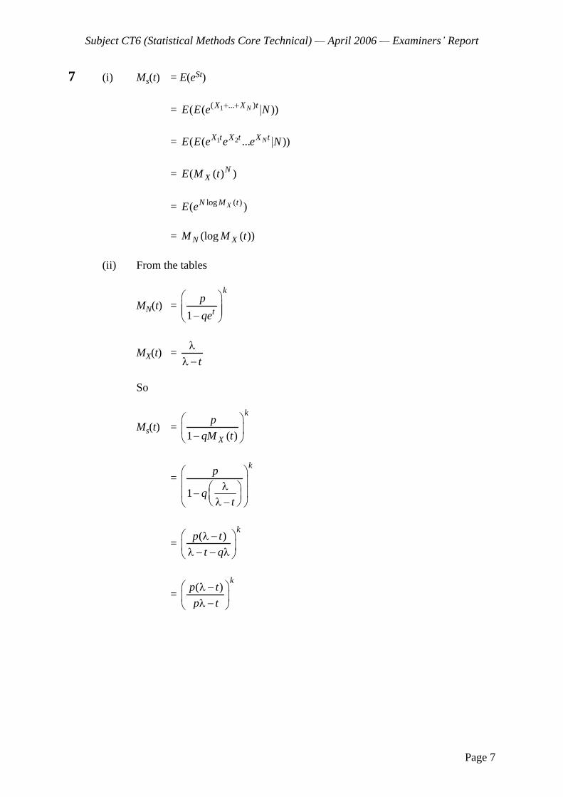
7 (i) Ms(t) = E(eSt)
= 1( ... )( ( ))NX X tE E e N
= 1 2( ( ... ))NX tX t X tE E e e e N
= ( ( ) )NXE M t
= log ( )( )XN M tE e
= (log ( ))N XM M t
(ii) From the tables
MN(t) = 1
k
t
p
qe
MX(t) = t
So
Ms(t) = 1 ( )
k
X
p
qM t
= 1
kp
qt
= ( )
kp t
t q
= ( )
kp t
p t

Subject CT6 (Statistical Methods Core Technical) April 2006
Examiners Report
Page 8
(iii) We now have
MY(t) = t
MR(t) = (p + qet)k
and so
MT(t) = k
p qt
= k
p pt q
t
= k
pt
t
Thus if we choose = p then MT(t) = MS(t) and by the uniqueness of Moment Generating Functions, S and T have the same distribution.
Comments on question 7: This question was generally well answered although relatively few managed the final step of demonstrating that S and T have the same distribution.
8 (i) The total number of claims has a Poisson distribution with parameter (n1 + n2) .
(ii) Let Yi denote the average total claim amount per policy in year i and let Xi
denote the total number of claims in year i. Then Xi has a Poisson distribution
with parameter ni and
X1 = 1 1n Y
c and X2 = 2 2 .
(1 )
Y n
c r
f( y1, y2)
f(y1, y2 ) f( )
1 1 1 2 2 2/ / (1 ) 11 2( ) ( )n y n c n y n c re n e n e
1 1 2 2
1 21
(1 )( )
n y n y
c c rn ne
So the posterior distribution of is gamma with parameters 1 1 2 2
(1 )
n y n y
c c r
and + n1 + n2.

Subject CT6 (Statistical Methods Core Technical) April 2006
Examiners Report
Page 9
(iii) E(Y3 y1, y2) = 2
3
(1 )c r
n
E(X3 y1, y2)
= 2
3
(1 )c r
n
n3
1 1 2 2
1 2
(1 )n y n y
c c rn n
= 2 2
1 1 2 2
1 2
(1 ) (1 ) (1 )c r n y r n y r
n n
= 2
2 1 1 2 2 1 2
1 2 1 2 1 2
(1 ) (1 )(1 )
n y r n y r n nc r
n n n n n n
k = 2
1 1 2 2
1 2
(1 ) (1 )n y r n y r
n n and
Z = 1 2
1 2
n n
n n
(iv) k is effectively a weighted average of the inflation adjusted average claim amounts for the previous 2 years, weighted by the number of policies in force. As the number of policies in force increases, Z becomes closer to 1, and so more weight is placed on the actual experience, and less on the prior expectations.
Comments on question 8: Candidates found this the most difficult question in the paper. Only those candidates with a methodical approach and an excellent grasp of the relevant bookwork managed to progress to the later parts of the question.
9 (i) Each entry can be expressed as:
Cij = rj . si . xi+j + eij
where:
rj is the development factor for year j, representing the proportion of claim payments by year j. Each rj is independent of the accident year i
si is a parameter varying by origin year, i, representing the exposure, for example the number of claims incurred in the accident year i

Subject CT6 (Statistical Methods Core Technical) April 2006
Examiners Report
Page 10
xi+j is a parameter varying by calendar year, for example representing inflation
eij is an error term
(ii) The cumulative cost of claims paid is:
Accident Year Development Year
0 1 2 3
2002 2,905 3,440 3,639 3,695 2003 3,315 3,893 4,052 2004 3,814 4,507 2005 4,723
The number of accumulated settled claims is as follows:
(Figures in £000s)
Accident Year Development Year
0 1 2 3 Ult
2002 430 (84.0%) 481 (93.9%) 505 (98.6%) 512 (100%) 512 2003 465 (83.8%) 523 (94.3%) 547 (98.6%) 554.8 2004 501 (84.2%) 560 (94.1%) 595.1 2005 539 (84.0%) 641.7
Average cost per settled claim:
Accident Year Development Year
0 1 2 3 Ult
2002 6.756 (93.6%) 7.152 (99.1%) 7.206 (99.8%) 7.217 (100%) 7.217 2003 7.129 (96.0%) 7.444 (100.3%) 7.408 (99.8%) 7.419 2004 7.613 (94.3%) 8.048 (99.7%) 8.072 2005 8.763 (94.7%) 9.256
Subject CT6 (Statistical Methods Core Technical) April 2006
Examiners Report
Page 11
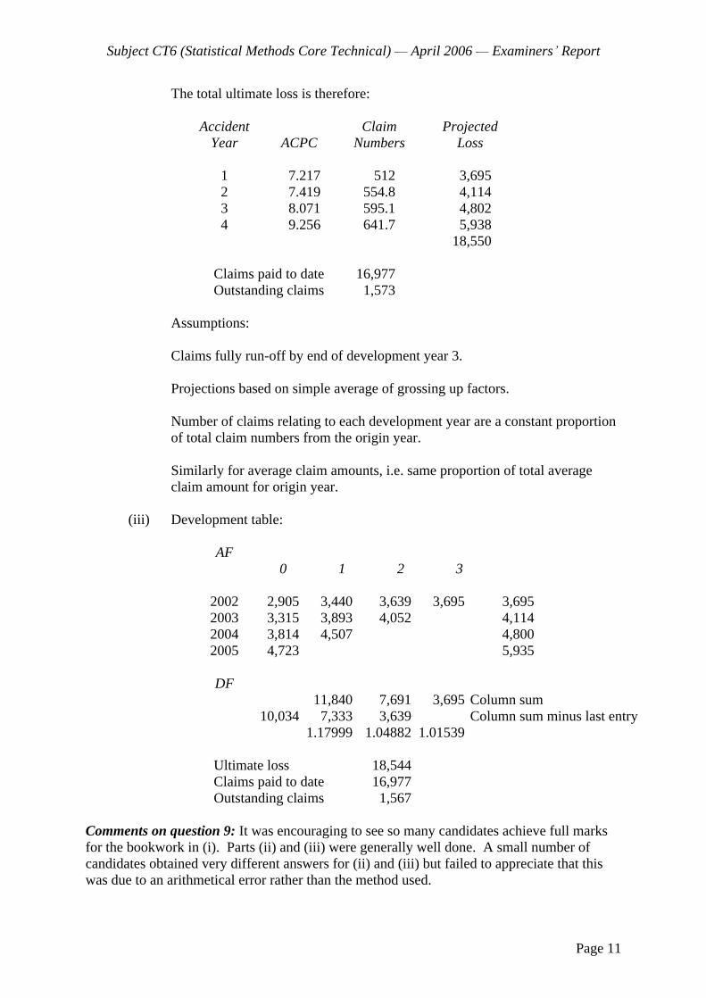
The total ultimate loss is therefore:
Accident Claim Projected Year ACPC Numbers Loss
1 7.217 512 3,695 2 7.419 554.8 4,114 3 8.071 595.1 4,802 4 9.256 641.7 5,938
18,550
Claims paid to date 16,977 Outstanding claims 1,573
Assumptions:
Claims fully run-off by end of development year 3.
Projections based on simple average of grossing up factors.
Number of claims relating to each development year are a constant proportion of total claim numbers from the origin year.
Similarly for average claim amounts, i.e. same proportion of total average claim amount for origin year.
(iii) Development table:
AF 0 1 2 3
2002 2,905 3,440 3,639 3,695 3,695 2003 3,315 3,893 4,052 4,114 2004 3,814 4,507 4,800 2005 4,723 5,935
DF 11,840 7,691 3,695 Column sum
10,034 7,333 3,639 Column sum minus last entry 1.17999 1.04882 1.01539
Ultimate loss 18,544 Claims paid to date 16,977 Outstanding claims 1,567
Comments on question 9: It was encouraging to see so many candidates achieve full marks for the bookwork in (i). Parts (ii) and (iii) were generally well done. A small number of candidates obtained very different answers for (ii) and (iii) but failed to appreciate that this was due to an arithmetical error rather than the method used.

Subject CT6 (Statistical Methods Core Technical) April 2006
Examiners Report
Page 12
10 (i) E(S) = E[S1] + E[S2]
= 10 5,000 + 30 4,000 = 170,000
Var[S] = Var[S1] + Var[S2]
= 10 5,0002 + 30 (4,0002 + 4,0002) = 1.21 109
(ii) We require u such that
P(u + c < S) = 0.01
i.e. ( ) ( )
Var( ) Var( )
S E S u c E SP
S S = 0.01
so ( )
Var( )
u c E S
S = 2.326
u = 2.326 Var( ) ( ) 1.1 ( )S E S E S
= 2.326 Var( ) 0.1 ( )S E S
= 63,922
(iii) We require u such that
( )R IP u c c S = 0.01
where cR = reinsurance premium
[ ]
Var[ ]R I
I
u c c E S
S = 2.326 =
[ ]
Var( )
u c E S
S
E[SI] = E[S] and Var[SI] = 2Var[S].
cR = (1 + )(1
) E[S]
Hence 1.1 [ ] (1 )(1 ) [ ] [ ]
Var[ ]
u E S E S E S
S =
1.1 [ ] [ ]
Var( )
u E S E S
S
u
= (u + 0.1E[S]) 1.1E[S] + (1 + )(1
) E[S] + E[S] = u + (0.1
1.1 + 1
+ (1
) + ) E(S) = u + (1
) (
0.1) E(S)

Subject CT6 (Statistical Methods Core Technical) April 2006
Examiners Report
Page 13
(iv) u u = (1
)[u (
0.1) E(S)]
0u u u (
0.1) E(S) > 0
i.e. < 0.1( )
u
E S
i.e. < 63,922
0.1170,000
= 0.476
(v) Since (1
) E[S] > 0, u
u decreases as increases.
The greater the premium loading required by the reinsurer, the smaller the reduction in capital required by the insurer, i.e. the less effective the reinsurance is in reducing P(ruin) and hence replacing the capital.
Comments on question 10: After Q8, candidates found this the most difficult question on the paper. Parts (i) and (ii) were well answered but the inclusion of premium loadings confused most candidates and consequently very few scored well on (iii), (iv) and (v).
END OF MARKING SCHEDULE

Faculty of Actuaries Institute of Actuaries
EXAMINATION
5 September 2006 (am)
Subject CT6 Statistical Methods Core Technical
Time allowed: Three hours
INSTRUCTIONS TO THE CANDIDATE
1. Enter all the candidate and examination details as requested on the front of your answer booklet.
2. You must not start writing your answers in the booklet until instructed to do so by the supervisor.
3. Mark allocations are shown in brackets.
4. Attempt all 10 questions, beginning your answer to each question on a separate sheet.
5. Candidates should show calculations where this is appropriate.
Graph paper is not required for this paper.
AT THE END OF THE EXAMINATION
Hand in BOTH your answer booklet, with any additional sheets firmly attached, and this question paper.
In addition to this paper you should have available the 2002 edition of the Formulae and Tables and your own electronic calculator.
Faculty of Actuaries CT6 S2006 Institute of Actuaries
CT6 S2006 2
1 The loss function under a decision problem is given by:
1 2 3
D1 11 9 19 D2 10 13 17 D3 7 13 10 D4 16 5 13
(i) State which decision can be discounted immediately and why. [2]
(ii) Explain what is meant by the minimax criterion and determine the minimax solution in this case. [2]
[Total 4]
2 A sequence of pseudo-random numbers from a uniform distribution over the interval [0, 1] has been generated by a computer.
(i) Explain the advantage of using pseudo-random numbers rather than generating a new set of random numbers each time. [1]
(ii) Use examples to explain how a sequence of pseudo-random numbers can be used to simulate observations from:
(a) a continuous distribution (b) a discrete distribution [4]
[Total 5]
3 State the Markov property and explain briefly whether the following processes are Markov:
AR(4); ARMA (1, 1).
[5]
4 An insurer insures a single building. The probability of a claim on a given day is p independently from day to day. Premiums of 1 unit are payable on a daily basis at the start of each day. The claim size is independent of the time of the claim and follows an exponential distribution with mean 1/ . The insurer has a surplus of U at time zero.
(i) Derive an expression for the probability that the first claim results in the ruin of the insurer. [6]
(ii) If p = 0.01 and = 0.0125 find how large U must be so that the probability that the first claim causes ruin is less than 1%. [2]
[Total 8]

CT6 S2006 3 PLEASE TURN OVER
5 (i) Let p be an unknown parameter, and let f(p x) denote the probability density of the posterior distribution of p given information x. Show that under all-or-nothing loss the Bayes estimate of p is the mode of f(p x). [2]
(ii) Now suppose p is the proportion of the population carrying a particular genetic condition. Prior beliefs about p have a U(0, 1) distribution. A sample of size N is taken from the population revealing that m individuals have the genetic condition.
(a) Suggest why the U(0, 1) distribution has been chosen as the prior, and derive the posterior distribution of p.
(b) Calculate the Bayes estimate of p under all-or-nothing loss. [6]
[Total 8]
6 The table below shows cumulative paid claims and premium income on a portfolio of general insurance policies.
Underwriting Development Year Premium Year 0 1 2 Income
2002 38,419 77,112 91,013 120,417 2003 31,490 78,504 117,101 2004 43,947 135,490
(i) Assuming an ultimate loss ratio of 93% for underwriting years 2003 and 2004, calculate the Bornhuetter-Ferguson estimate of outstanding claims for this triangle. [8]
(ii) State the assumptions underlying this estimate. [2] [Total 10]

CT6 S2006 4
7 The random variable W has a binomial distribution such that
P(W = w) = n
w
w (1 )n w (w = 0, 1, 2, , n)
Let Y = W
n.
(i) Write down an expression for P(Y = y), for y = 0, 1 2
, ,...,1n n
. [1]
(ii) Express the distribution of Y as an exponential family and identify the natural parameter and the dispersion parameter. [3]
(iii) Derive an expression for the variance function. [3]
(iv) For a set of n independent observations of Y, derive an expression of the scaled deviance. [3]
[Total 10]
8 (i) Let X denote the claim amount under an insurance policy, and suppose that X has a probability density fX(x) for x > 0. The insurer has an individual excess of loss reinsurance arrangement with a retention of £M. Let Y be the amount paid by the insurer net of reinsurance. Express Y in terms of X and hence derive an expression for the probability density function of Y in terms of fX(x).
[3]
For a particular class of policy X is believed to follow a Weibull distribution with probability density function
fX(x) = 0.75cx 0.250.75cxe (x > 0)
where c is an unknown constant. The insurer has an individual excess of loss reinsurance arrangement with retention £500. The following claims data are observed:
Claims below retention: 78, 104, 116, 135, 189, 243, 270, 350, 411, 491 Claims above retention: 3 in total Total number of claims: 13
(ii) Estimate c using maximum likelihood estimation. [7]
(iii) Apply the method of percentiles using the median claim to estimate c. [4] [Total 14]

CT6 S2006 5 PLEASE TURN OVER
9 An insurer operates a No Claims Discount system with three levels of discount:
Discount
Level 0 0% Level 1 20% Level 2 50%
The annual premium in level 0 is £650.
If a policyholder makes no claims in a policy year, they move to the next high discount level (or remain at level 2). In all other cases they move to (or remain at) discount level 0.
For a policyholder who has not yet had an accident in a policy year, the probability of an accident occurring is 0.1. The time at which an accident occurs in the policy year is denoted by T, where
0
T 1; T = 0 means that the accident occurs at the start of the policy year; T = 1 means that the accident occurs at the end of the policy year.
It is assumed that T has a uniform distribution.
Given that a policyholder has had their first accident, the probability of them having a second accident in the same policy year is 0.4(1
T). It is assumed that a policyholder will not have more than two accidents in a policy year.
The cost of each accident has an exponential distribution with mean £1,000.
After each accident, the policyholder decides whether or not to make a claim by comparing the increase in the premium they would have to pay in the next policy year with the claim size. In doing this, they assume that they will have no further accidents.
(i) Show that the distribution of the number of accidents, K, that a policyholder has in a year is:
P(K = 0) = 0.9 P(K = 1) = 0.08 P(K = 2) = 0.02
[4]
(ii) For each level of discount, calculate the probability that a policyholder makes n claims in a policy year, where n = 0, 1, 2. [8]
(iii) Write down the transition matrix. [2]
(iv) Derive the steady state distribution. [3] [Total 17]

CT6 S2006 6
10 (i) Let Ik = k x
mx e dx
where k is a non-negative integer.
Show that I0 = 1 me
and Ik = 1
km
km k
e I (k = 1, 2, 3, ) [3]
For a certain portfolio of insurance policies the number of claims annually has a Poisson distribution with mean 25. Claim sizes have a gamma distribution with mean 100 and variance 5,000 and the insurer includes a loading of 10% in its premium.
The insurer is considering purchasing individual excess of loss reinsurance with retention m from a reinsurer that includes a loading of 15% in its premium.
Let XI and XR denote the amounts paid by the direct insurer and the reinsurer, respectively, on an individual claim.
(ii) Calculate the premium, c, charged by the direct insurer for this portfolio. [1]
(iii) Show that E[XR] = 2
1
50 (I2
mI1) and hence that
E[XR] = (m + 100) e m/50. [7]
(iv) Use the result in (iii) to derive an expression for E[XI]. [1]
(v) Derive an expression for the direct insurer s expected annual profit. [3]
(vi) The table below shows the direct insurer s expected annual profit (Profit) and probability of ruin (P(ruin)), for various values of the retention level, m:
m Profit P(ruin)
36 1.8 0.002 50 * 0.01
100 148.5 0.05
Calculate the missing value in the table and discuss the issues facing the direct insurer when deciding on the retention level to use. [4]
[Total 19]
END OF PAPER
Faculty of Actuaries Institute of Actuaries
EXAMINATION
September 2006
Subject CT6 — Statistical Methods Core Technical
EXAMINERS’ REPORT
Introduction The attached subject report has been written by the Principal Examiner with the aim of helping candidates. The questions and comments are based around Core Reading as the interpretation of the syllabus to which the examiners are working. They have however given credit for any alternative approach or interpretation which they consider to be reasonable. M A Stocker Chairman of the Board of Examiners November 2006
© Faculty of Actuaries © Institute of Actuaries

Subject CT6 (Statistical Methods Core Technical) — September 2006 — Examiners’ Report
Page 2
Comments Comments on solutions presented to individual questions for this September 2006 paper are given below. Question 1 Consistently well answered. Question 2 Generally well answered, though a number of candidates did not produce an example for the discrete case. Question 3 Most candidates dealt with AR(4) well. However, most thought that ARMA(1,1) was Markov. Many of those who knew it is not Markov did not explain why it is not. Question 4 Candidates found this the hardest question on the paper, with the vast majority struggling to score many marks. Most candidates did not make the first step of conditioning on the time to the first claim, and therefore made little if any progress with the question. Question 5 Many candidates did not recall the bookwork in part (i). The standard of answers to part (ii) was nevertheless good. Question 6 Generally very well answered, although a number of candidates failed to explicitly state the outstanding claims and therefore did not score full marks. Question 7 Parts (i) and (ii) were consistently well answered. Stronger candidates also scored well on parts (iii) and (iv). Question 8 This question was a good differentiator — whilst weaker candidates struggled, better candidates were able to score well, the main difficulties being specifying the distribution of Y in part (i) and dealing with the claims above the retention in part (ii).

Subject CT6 (Statistical Methods Core Technical) — September 2006 — Examiners’ Report
Page 3
Question 9 Only a few candidates were sufficiently methodical in their approach to part (ii) and therefore gained full marks on this question. Nevertheless, many candidates scored well on the question overall, in particular picking up the follow-on marks available in parts (iii) and (iv). A number of candidates found the link between losses and claims confusing and therefore interpreted the question in a way that that made it more complicated than it actually was. Question 10 This was well answered overall, with many candidates scoring well, especially on parts (i) to (iv). Only the best candidates scored highly on part (vi).

Subject CT6 (Statistical Methods Core Technical) — September 2006 — Examiners’ Report
Page 4
1 (i) D2 can be eliminated since it is dominated by D3; that is under all circumstances the loss from D2 is greater than or equal to that from D3.
(ii) The minimax criterion is to choose D so that the loss, maximised with respect
to theta, is a minimum. The relevant maximum losses are D1 19 D3 13 D4 16 So we should chose D3. 2 (i) Using pseudo-random numbers removes the variability of using different sets
of random numbers, which is helpful for comparing different models. Only a single routine is required for generation of pseudo-random numbers
whereas in the case of truly random numbers we need either a lengthy table or a hardware enhancement to a computer.
If we wish to use the same sequence of random numbers in 2 models we need
only store the seed for the pseudo-random random numbers as opposed to a record of potentially millions of truly random numbers.
(ii) u is a random number from U(0, 1) (a) Find x from u = F(x) so x = F−1(u). e.g. exponential u = e−λx
x = logu−λ
(b) Working with integers, find x such that P(X ≤ x − 1) < u ≤ P(X ≤ x) e.g. toss a coin, X = number of heads X = 0 if u ≤ 0.5, X = 1 otherwise

Subject CT6 (Statistical Methods Core Technical) — September 2006 — Examiners’ Report
Page 5
3 The Markov property for a process {Yt} states that the conditional distribution of Yt|Yt−1 is the same as the conditional distribution of
Yt|Yt−1, Yt−2, … Development can be predicted from present state without any reference to past
history. AR(4) Yt = α + β1Yt−1 + β2Yt−2 + β3Yt−3 + β4Yt−4 + et This is not Markov since the distribution of Yt|Yt−1 changes when Yt−2, Yt−3, Yt−4 are
also given. ARMA(1,1) Yt = α + βYt−1 + et − θet−1 Yt−1 = α + βYt−2 + et−1 − θet−2 Hence et−1 = Yt−1 − α − βYt−2 + θet−2, and substituting into the expression for Yt, it
can be seen that knowledge of Yt−2 changes the distribution of Yt|Yt−1. So this is not Markov.
4 (i) P(ruin on 1st claim)= ( )
0First claim at
tP t
>∑ × P(this claim causes ruin)
= 1
0
t
tq −
>∑ × p × P(this claim > U + t)
= 1
0
t x
t U t
pq e dx∞
− −λ
> +
× λ∑ ∫
= 1
0
t xU tt
pq e∞− −λ
+>
⎡ ⎤× −⎣ ⎦∑
= 1 ( )
0
t U t
tpq e− −λ +
>∑
= 1
0
t U t
tpq e e− −λ −λ
>∑

Subject CT6 (Statistical Methods Core Technical) — September 2006 — Examiners’ Report
Page 6
= 1
0( )U t
tpe e qe−λ −λ −λ −
>∑
=( 1)
1
Upeqe
−λ +
−λ−
(ii) We want
0.0125( 1)
0.01250.01 0.011 0.99
Uee
− +
−×
<− ×
hence
0.01250.009875778 0.01
0.022297977
Ue−×<
i.e. e−0.0125U < 0.02257845 taking logarithms −0.0125U < −3.79076 so that we require U > 303.26 5 (i) Consider the loss function
L(g(x), p) = 0 if1 otherwise
g p g− ε < < + ε⎧⎨⎩
Then the expected posterior loss is given by
1 ( )g
g
f p x dp+ε
−ε
− ∫ ⏐
≈ 1 − 2εf(g|x) for small values of ε. This is minimised by setting g to be the maximum (i.e.
the mode) of f(p|x).

Subject CT6 (Statistical Methods Core Technical) — September 2006 — Examiners’ Report
Page 7
(ii) (a) Using U(0, 1) as the prior for p suggests that no prior information or beliefs about p have been formed — it is equally likely to lie anywhere in the range [0, 1].
f(p|m) ∝ f(m|p) f(p) ∝ pm(1 − p)N−m × 1 So posterior beliefs about p have a Beta distribution with parameters
m + 1 and N − m + 1. (b) We must find the mode of (f(p|m). Maximising this is the same as maximising g(p) = log f(p|m) = m log p + (N − m) log (1 − p) + constant
( )g p′ = 1
m N mp p
−−
−
and ( )g p′ = 0 when
1
m N mp p
−−
− = 0 i.e.
m(1 − p) = (N − m) p Np = m p = m / N

Subject CT6 (Statistical Methods Core Technical) — September 2006 — Examiners’ Report
Page 8
6 (i) Column totals: 155,616 91,013 Column totals excluding last entry: 69,909 77,112 Development factors: 2.2260 1.1803 f: 2.6273 1.1803 Underwriting Year Premium Initial UL 2003 117,101 108,904 2004 135,490 126,006 Emerging Initial UL f 1 − 1/f Liability 2003 108,904 1.1803 0.1527 16,634 2004 126,006 2.6273 0.6194 78,045 So the estimate of outstanding claims is 94,678. (ii) Assumptions: Data already adjusted for inflation or past pattern of inflation will be repeated
in future. Payment pattern same for each underwriting year. Estimated Loss Ratio is appropriate. Claims from underwriting year 2002 are fully run off.
7 (i) P(Y = y) = nny
⎛ ⎞⎜ ⎟⎝ ⎠
μny (1 − μ)n−ny
(ii) P(Y = y) = exp log (1 ) log(1 ) logn
ny n yny
⎡ ⎤⎛ ⎞μ + − − μ +⎢ ⎥⎜ ⎟
⎝ ⎠⎣ ⎦
= exp log log(1 ) log1
nn y
ny⎡ ⎤⎛ ⎞⎛ ⎞μ
+ − μ +⎢ ⎥⎜ ⎟⎜ ⎟− μ⎝ ⎠ ⎝ ⎠⎣ ⎦
which is in the form of an exponential family.
The natural parameter is log1
μ− μ
.
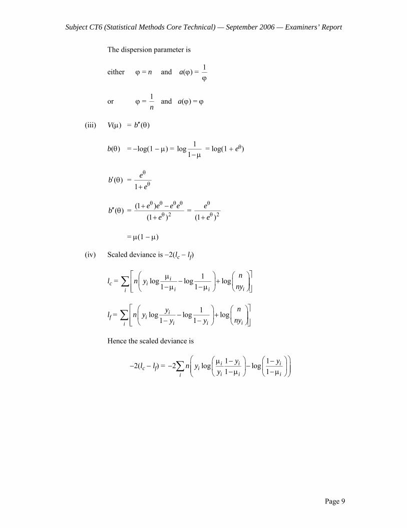
Subject CT6 (Statistical Methods Core Technical) — September 2006 — Examiners’ Report
Page 9
The dispersion parameter is
either ϕ = n and a(ϕ) = 1ϕ
or ϕ = 1n
and a(ϕ) = ϕ
(iii) V(μ) = ( )b′′ θ
b(θ) = −log(1 − μ) = 1log1− μ
= log(1 + eθ)
( )b′ θ = 1
ee
θ
θ+
( )b′′ θ = 2(1 )
(1 )e e e e
e
θ θ θ θ
θ+ −
+ = 2(1 )
ee
θ
θ+
= μ(1 − μ) (iv) Scaled deviance is −2(lc − lf)
lc = 1log log log1 1
ii
ii ii
nn y
ny⎡ ⎤⎛ ⎞ ⎛ ⎞μ
− +⎢ ⎥⎜ ⎟ ⎜ ⎟− μ − μ⎢ ⎥⎝ ⎠⎝ ⎠⎣ ⎦∑
lf = 1log log log1 1
ii
ii ii
nyn ynyy y
⎡ ⎤⎛ ⎞ ⎛ ⎞− +⎢ ⎥⎜ ⎟ ⎜ ⎟− −⎢ ⎥⎝ ⎠⎝ ⎠⎣ ⎦
∑
Hence the scaled deviance is
−2(lc − lf) = 1 12 log log1 1
i i ii
i i ii
y yn yy
⎛ ⎞⎛ ⎞ ⎛ ⎞μ − −− −⎜ ⎟⎜ ⎟ ⎜ ⎟⎜ ⎟− μ − μ⎝ ⎠ ⎝ ⎠⎝ ⎠
∑
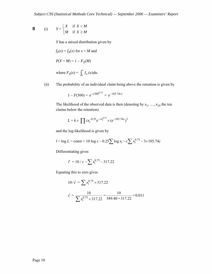
Subject CT6 (Statistical Methods Core Technical) — September 2006 — Examiners’ Report
Page 10
8 (i) Y = ifif
X X MM X M
<⎧⎨ ≥⎩
Y has a mixed distribution given by fY(x) = fX(x) for x < M and P(Y = M) = 1 − FX(M) where FX(x) =
0( ) .
x
Xf u du∫
(ii) The probability of an individual claim being above the retention is given by 1 − F(500) =
0.75500ce− = 105.74 ce− × The likelihood of the observed data is then (denoting by x1, …, x10 the ten
claims below the retention) L = k ×
0.750.25 105.74 3( )icx cicx e e−− −×∏
and the log-likelihood is given by l = log L = const + 10 log c − 0.750.25 log 3 105.74i ix c x c− − ×∑ ∑ Differentiating gives l′ = 10 / c 0.75 317.22ix− −∑ Equating this to zero gives ˆ10 / c = 0.75 317.22ix +∑
c = 0.7510 10= = 0.011
589.40 + 317.22317.22ix +∑
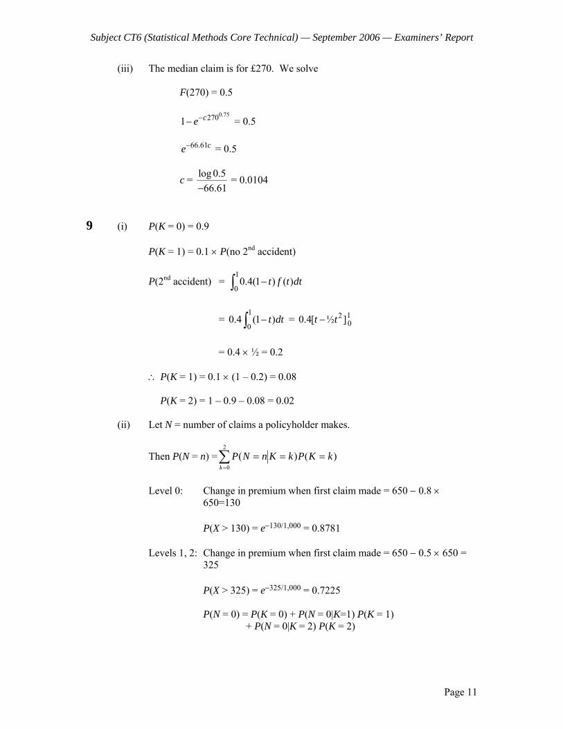
Subject CT6 (Statistical Methods Core Technical) — September 2006 — Examiners’ Report
Page 11
(iii) The median claim is for £270. We solve F(270) = 0.5
0.752701 ce−− = 0.5 66.61ce− = 0.5
c = log 0.566.61−
= 0.0104
9 (i) P(K = 0) = 0.9 P(K = 1) = 0.1 × P(no 2nd accident)
P(2nd accident) = 1
00.4(1 ) ( )t f t dt−∫
= 1
00.4 (1 )t dt−∫ = 12
00.4[ ½ ]t t−
= 0.4 × ½ = 0.2 ∴ P(K = 1) = 0.1 × (1 – 0.2) = 0.08 P(K = 2) = 1 – 0.9 – 0.08 = 0.02 (ii) Let N = number of claims a policyholder makes.
Then P(N = n) =∑=
===2
0)()(
kkKPkKnNP
Level 0: Change in premium when first claim made = 650 − 0.8 ×
650=130 P(X > 130) = e−130/1,000 = 0.8781 Levels 1, 2: Change in premium when first claim made = 650 − 0.5 × 650 =
325 P(X > 325) = e−325/1,000 = 0.7225 P(N = 0) = P(K = 0) + P(N = 0|K=1) P(K = 1) + P(N = 0|K = 2) P(K = 2)

Subject CT6 (Statistical Methods Core Technical) — September 2006 — Examiners’ Report
Page 12
Level 0: P(N = 0) = 0.9 + 0.1219 × 0.08 + 0.12192 × 0.02 = 0.9100 Levels 1, 2: P(N = 0) = 0.9 + 0.2775 × 0.08 + 0.27752 × 0.02 = 0.9237
Note that if one claim has already been made then the NCD has already been lost, and it is therefore certain that a second claim will be made, regardless of the size of the loss. Therefore, for two accidents to result in only one claim it must be that the first accident resulted in no claim, and the second resulted in a claim.
P(N = 1) = P(N = 1|K = 1) P(K = 1) + P(N = 1|K = 2) P(K = 2) Level 0: P(N = 1) = 0.8781 × 0.08 + 0.1219× 0.8781 × 0.02 = 0.0724 Levels 1, 2: P(N = 1) = 0.7225 × 0.08 + 0.2775 × 0.7255 × 0.02 = 0.0618 Two accidents will result in two claims whenever the first accident results in a
claim (since in this case the second accident will certainly result in a claim). P(N = 2) = P(N = 2|K = 2) P(K = 2) Level 0: 0.8781 × 0.02 = 0.0176 Levels 1, 2: P(N = 2) = 0.7225 × 0.02 = 0.0145 (iii) The transition matrix is
0.0900 0.9100 00.0762 0 0.92380.0762 0 0.9238
⎛ ⎞⎜ ⎟⎜ ⎟⎜ ⎟⎝ ⎠
(iv) ππ P= 0.9100π0 = π1 0.9238(π1+ π2) = π2 ∴ π2 = 12.123π1 = 11.032π0

Subject CT6 (Statistical Methods Core Technical) — September 2006 — Examiners’ Report
Page 13
Since π0 + π1 + π2 = 1 π0 + 0.9100π0 + 11.032π0 = 1 ∴ π0 = 0.0773, π1 = 0.0703, π2 = 0.8524
10 (i) I0 = xm
e dx∞ −β∫ = 1 x
me
∞−β⎡ ⎤
−⎢ ⎥β⎣ ⎦= 1 me−β
β
Ik = k xm
x e dx∞ −β∫ =
11 kk x x
mm
kxx e e dx∞ −∞−β −β⎡ ⎤
− +⎢ ⎥β β⎣ ⎦ ∫
= 1k
m k xm
m ke x e dx∞−β − −β+
β β ∫
= 1
km
km ke I−β
−+β β
(ii) c = 1.1 × 25 × 100 = 2,750
(iii) E[XR] = ( ) ( )m
x m f x dx∞
−∫
f(x) is gamma, and αβ
= 100, 2αβ
= 5,000
∴β = 150
and α = 2
∴ f(x) = 2
501 ( 0)50
xxe x−⎛ ⎞ >⎜ ⎟
⎝ ⎠
E[XR] = 2 / 50 / 502
150
x xm m
x e dx m xe dx∞ ∞− −⎡ ⎤−⎢ ⎥⎣ ⎦∫ ∫
= 2 121 [ ]
50I mI−
I0 = 50e−m/50
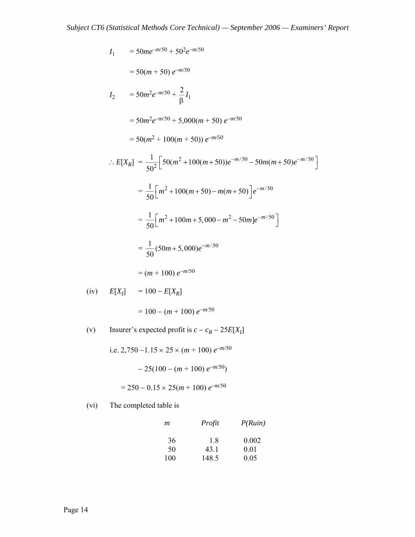
Subject CT6 (Statistical Methods Core Technical) — September 2006 — Examiners’ Report
Page 14
I1 = 50me−m/50 + 502e−m/50 = 50(m + 50) e−m/50
I2 = 50m2e−m/50 + 12 Iβ
= 50m2e−m/50 + 5,000(m + 50) e−m/50 = 50(m2 + 100(m + 50)) e−m/50
∴E[XR] = 2 /50 / 502
1 50( 100( 50)) 50 ( 50)50
m mm m e m m e− −⎡ ⎤+ + − +⎣ ⎦
= 2 / 501 100( 50) ( 50)50
mm m m m e−⎡ ⎤+ + − +⎣ ⎦
= 2 2 / 501 100 5,000 50 ]50
mm m m m e−⎡ ⎤+ + − −⎣ ⎦
= / 501 (50 5,000)50
mm e−+
= (m + 100) e−m/50 (iv) E[XI] = 100 − E[XR] = 100 − (m + 100) e−m/50 (v) Insurer’s expected profit is c − cR − 25E[XI] i.e. 2,750 −1.15 × 25 × (m + 100) e−m/50 − 25(100 − (m + 100) e−m/50) = 250 − 0.15 × 25(m + 100) e−m/50 (vi) The completed table is m Profit P(Ruin) 36 1.8 0.002 50 43.1 0.01 100 148.5 0.05
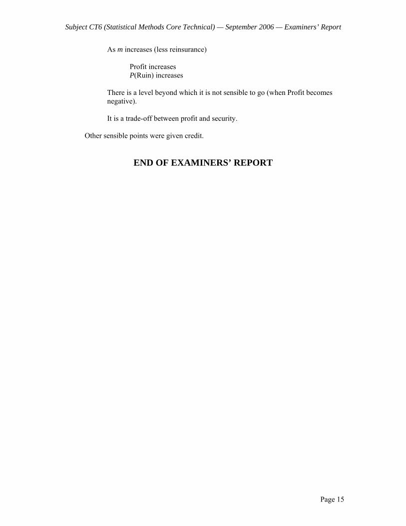
Subject CT6 (Statistical Methods Core Technical) — September 2006 — Examiners’ Report
Page 15
As m increases (less reinsurance) Profit increases P(Ruin) increases There is a level beyond which it is not sensible to go (when Profit becomes
negative). It is a trade-off between profit and security. Other sensible points were given credit.
END OF EXAMINERS’ REPORT

Faculty of Actuaries Institute of Actuaries
EXAMINATION
19 April 2007 (am)
Subject CT6 — Statistical Methods Core Technical
Time allowed: Three hours
INSTRUCTIONS TO THE CANDIDATE
1. Enter all the candidate and examination details as requested on the front of your answer booklet.
2. You must not start writing your answers in the booklet until instructed to do so by the
supervisor. 3. Mark allocations are shown in brackets. 4. Attempt all 11 questions, beginning your answer to each question on a separate sheet. 5. Candidates should show calculations where this is appropriate.
Graph paper is not required for this paper.
AT THE END OF THE EXAMINATION
Hand in BOTH your answer booklet, with any additional sheets firmly attached, and this question paper.
In addition to this paper you should have available the 2002 edition of the Formulae and Tables and your own electronic calculator.
© Faculty of Actuaries CT6 A2007 © Institute of Actuaries
CT6 A2007—2
1 (i) State two conditions for a risk to be insurable. [2] (ii) Describe briefly three distinct examples of financial loss insurance policies. [3] [Total 5] 2 (i) Explain the concept of cointegrated time series. [3] (ii) Give two examples of circumstances when it is reasonable to expect that two
processes may be cointegrated. [2] [Total 5] 3 The random variable X has an exponential distribution with mean 1000. Individual
claim amounts on a certain type of insurance policy, Y, are such that Y X= for 0 2000X< < and ( ) ( )2000 2000P Y P X= = ≥ . The insurer applies a deductible of 100 on claims from this type of insurance. Calculate the mean of the distribution of individual claim amounts paid by the insurer. [5]
CT6 A2007—3 PLEASE TURN OVER
4 A casino operator moving into a country for the first time must apply to the casino regulator for a licence. There are three types of licence to choose from — slots, dice and cards — each with different running costs. The casino operator has to pay a fixed amount annually (£1,300,000) to the regulator, plus a variable annual licence cost.
The variable licence cost and expected revenue per customer for each type of game
are as follows:
Variable Licence cost
£
Expected Revenueper customer
£
Slots 250,000 60 Dice 550,000 120 Cards 1,150,000 160
The casino operator is uncertain about the number of customers and decides to
prepare a profit forecast based on cautious, best estimate and optimistic numbers of customers. The figures are 14,000; 20,000 and 23,000 respectively.
(i) Determine the annual profits under each possible combination. [2]
(ii) Determine the minimax solution for optimising the profits. [2]
(iii) Determine the Bayes criterion solution based on the annual profit given the probability distribution P(cautious) = 0.2, P(best estimate) = 0.7 and P(optimistic) = 0.1. [2]
[Total 6]
CT6 A2007—4
5 The delay triangles given below relate to a portfolio of motor insurance policies. The cost of claims settled during each year is given in the table below: (Figures in £000s)
Development year Accident
Year
0 1 2
2004 4,144 694 183 2005 4,767 832 2006 5,903
The corresponding number of settled claims is as follows:
Development year Accident
Year 0 1 2
2004 581 75 28 2005 626 71 2006 674
Calculate the outstanding claims reserve for this portfolio using the average cost per
claim method with grossing-up factors, and state the assumptions underlying your result.
[7] 6 (i) Explain the main advantage of the Polar method compared with the Box-
Muller method for generating pairs of uncorrelated pseudo-random values from a standard normal distribution. [2]
(ii) Pseudo-random numbers are generated using the Box-Muller method in order
to simulate values of Y X= , where X has a lognormal distribution with parameters μ = 5 and σ = 2. The quantity of interest is [ ]E Yθ = .
(a) Calculate the value of Y when the number generated by the Box-Muller
method is 0.9095. (b) The variance of Y has been estimated as 26.3. Calculate how many
simulations should be performed in order to ensure that the discrepancy between Y and θ , measured by the absolute error, is less than 1 with probability at least 0.9. [5]
[Total 7]

CT6 A2007—5 PLEASE TURN OVER
7 The total claims arising from a certain portfolio of insurance policies over a given month is represented by
1if 0
=
0 if = 0
N
ii
X NS
N=
⎧>⎪
⎨⎪⎩
∑
where N has a Poisson distribution with mean 2 and 1 2, , , NX X X… is a sequence of
independent and identically distributed random variables that are also independent of N. Their distribution is such that ( = 1) = 1/ 3 and ( = 2) = 2 / 3i iP X P X . An aggregate reinsurance contract has been arranged such that the amount paid by the reinsurer is S - 3 (if S > 3) and zero otherwise.
The aggregate claims paid by the direct insurer and the reinsurer are denoted by
andI RS S , respectively. Calculate ( ) and ( )I RE S E S . [8]

CT6 A2007—6
8 A modeller has attempted to fit an ARMA(p,q) model to a set of data using the Box-Jenkins methodology. The plot of residuals based on this proposed fit is shown below.
(i) Under the assumptions of the model, the residuals should form a white noise
process.
(a) By inspection of the chart, suggest two reasons to suspect that the residuals do not form a white noise process.
(b) Define what is meant by a turning point. (c) Perform a significance test on the number of turning points in the data
above. (There are 100 points in the data and 59 turning points.) [6] (ii) On your suggestion, the original fitted model is discarded, and re-
parameterised to: 2 1 2= 5 0.9( 5) 0.5n n n nX X e e+ + ++ − + + . Given the following observations:
99 100
99 100
= 2, = 7ˆ ˆ= 0.7, = 1.4
X Xe e−
Use the Box-Jenkins methodology to calculate the forward estimates
100 100(1), (2)X X and 100(3)X . [4] [Total 10]
Residuals based on fitted model
-80-60-40-20
020406080
100120
1 6 11 16 21 26 31 36 41 46 51 56 61 66 71 76 81 86 91 96
Time
CT6 A2007—7 PLEASE TURN OVER
9 An insurer’s NCD scale for motor policies has 3 levels of discount: 0%, 25% and 40%. The rules for moving between these levels are as follows:
• following a claim-free year, a policyholder moves to the next higher level of
discount, or remains at 40% discount • following a year of one or more claims, a policyholder at 40% discount moves to
25% discount while a policyholder at 25% or 0% moves to or stays at 0% discount
The full premium for each policyholder is £1,000. Following an accident, policyholders decide whether or not to claim by considering total outgoing over the next two years, assuming no further claims in this period and ignoring interest.
(i) Find the claim threshold for each level of discount. [3] (ii) The probability of no accidents in any year for each policyholder is 0.88 and
individual losses are assumed to have a lognormal distribution with μ = 6.0 and σ = 3.33. Ignoring the possibility of more than 1 accident occurring in a year, calculate the transition matrix. [3]
(iii) Calculate the stationary distribution. [3] (iv) Derive the stationary distribution under the alternative assumption that a
policyholder always claims after a loss (regardless of the size of the claim). [3] (v) Comment on the difference between the results of (iii) and (iv). [1] [Total 13]

CT6 A2007—8
10 (i) The Gamma distribution with mean μ and variance μ2/α has density function
f(y) = 1
( )
y
y eαα −
α− μαα
μ Γ α ( )0y >
(a) Show that this may be written in the form of an exponential family. (b) Use the properties of exponential families to confirm that the mean and
variance of the distribution are μ and μ2/α. [9] (ii) Explain the difference between a continuous covariate and a factor. [3] (iii) A company is analysing its claims data on a portfolio of motor policies, and
uses a gamma distribution to model the claim severities. The company uses three rating factors:
policyholder age (as a continuous variable); policyholder gender; vehicle rating group (as a factor). (a) Write down the form of the linear predictor when all rating factors are
included as main effects. (b) State how the linear predictor changes if an interaction between
policyholder age and gender is included. [4] [Total 16] 11 The number, X, of claims on a given insurance policy over one year has probability
distribution given by ( = ) = (1 ) = 0,1, 2,kP X k kθ − θ … where θ is an unknown parameter with 0 1< θ < . Independent observations 1, , nx x… are available for the number of claims in the
previous n years. Prior beliefs about θ are described by a distribution with density 1 1( ) (1 )f α− α−θ ∝ θ −θ for some constant 0α > .
CT6 A2007—9
(i) (a) Derive the maximum likelihood estimate, θ , of θ given the data 1, , nx x… .
(b) Derive the posterior distribution of θ given the data 1, , nx x… . (c) Derive the Bayesian estimate of θ under quadratic loss and show that
it takes the form of a credibility estimate ˆ (1 )Z Zθ+ − μ where μ is a quantity you should specify from the prior distribution of
θ. (d) Explain what happens to Z as the number of years of observed data
increases. [11] (ii) (a) Determine the variance of the prior distribution of θ. (b) Explain the implication for the quality of prior information of
increasing the value of α. Give an interpretation of the prior distribution in the special case α = 1.
[3] (iii) Calculate the Bayesian estimate of θ under quadratic loss if n = 3,
1 2 3= 3, = 3, = 5x x x and (a) α = 5 (b) α = 2 Comment on your results in the light of (ii) above. [4] [Total 18]
END OF PAPER

Faculty of Actuaries Institute of Actuaries
EXAMINATION
April 2007
Subject CT6 — Statistical Methods Core Technical
EXAMINERS’ REPORT
Introduction The attached subject report has been written by the Principal Examiner with the aim of helping candidates. The questions and comments are based around Core Reading as the interpretation of the syllabus to which the examiners are working. They have however given credit for any alternative approach or interpretation which they consider to be reasonable. M A Stocker Chairman of the Board of Examiners June 2007
© Faculty of Actuaries © Institute of Actuaries

Subject CT6 (Statistical Methods Core Technical) — April 2007 — Examiners’ Report
Page 2
Comments Comments on solutions presented to individual questions for this April 2007 paper are given below. Question 1 Generally well answered. Question 2 This bookwork question was poorly answered and only the best prepared candidates scored well. Question 3 Relatively few candidates correctly identified that the deductible of 100 applied to all claims Question 4 Most candidates scored full marks on this question. Question 5 Candidates generally scored well on this straightforward question Question 6 This was the most difficult question on the paper. Many answered the bookwork in part (i) but were unable to make a start on part (ii). Question 7 Poorly answered. Most candidates correctly calculated E(S) but failed to work methodically through the calculation of E(SI). Question 8 This question was a good differentiator — whilst weaker candidates struggled with (i)(c) and (ii),, Full credit was also given for those candidates who checked the probability that T>58.5 in (i)(c). Question 9 This was well answered. Question 10 Parts (i) and (ii) of this question were well answered on the whole. Only the best candidates answered part (iii) well. Question 11 Part (i) of this question was well answered. Only the best candidates scored the second mark in (ii)(b). Although many candidates achieved full marks for the calculation of θ* relatively few were awarded both marks for their comments in (iii).
Subject CT6 (Statistical Methods Core Technical) — April 2007 — Examiners’ Report
Page 3
1 (i) The policyholder must have an interest in the risk being insured, to distinguish between insurance and a wager.
The risk must be of a financial and reasonably quantifiable nature. (ii) Pecuniary loss — protects against bad debts or other failure of a third party. Fidelity guarantee — protects against losses caused by dishonest actions of
employees. Business interruption cover — protects against losses made as a result of not
being able to conduct business. 2 (i) Two time series X, Y are cointegrated if X and Y are I(1) random processes and there exists a non-zero vector (α, β) such that αX + βY is stationary. I(1) means that ∇X and ∇Y are stationary (α, β) is called a cointegrating vector (ii) Examples: One of the processes is driving the other Both are being driven by the same underlying process 3 The claim amount, Z, is given by
Z = 0100Y
⎧⎨ −⎩
100100
YY<≥
[ ] ( ) ( ) ( )2000
100100 1900 2000E Z x f x dx P X= − + ≥∫
2000 2000 2000
100 100100 1900x xx e dx e dx e−λ −λ − λ= λ − λ +∫ ∫
where 11000
λ =
Subject CT6 (Statistical Methods Core Technical) — April 2007 — Examiners’ Report
Page 4
Hence [ ]2000 20002000 2000
100100 100100 1900x x xE Z xe e dx e e−λ −λ −λ − λ⎡ ⎤ ⎡ ⎤= − + − − +⎣ ⎦ ⎣ ⎦∫
( )2000
100 2000 100 2000 2000
100
1100 2000 100 1900xe e e e e e− λ − λ −λ − λ − λ − λ⎡ ⎤= − + − − − +⎢ ⎥λ⎣ ⎦
( )100 20001 e e− λ − λ= −λ ( )0.1 21000 769.5e e− −= − = .
4 (i) Revenue (£)
Cautious Best estimate Optimistic
Slots 840,000 1,200,000 1,380,000 Dice 1,680,000 2,400,000 2,760,000 Cards 2,240,000 3,200,000 3,680,000
Costs (£)
Cautious Best estimate Optimistic
Slots 1,550,000 1,550,000 1,550,000 Dice 1,850,000 1,850,000 1,850,000 Cards 2,450,000 2,450,000 2,450,000
Profit (£)
Cautious Best estimate Optimistic
Slots -710,000 -350,000 -170,000 Dice -170,000 550,000 910,000 Cards -210,000 750,000 1,230,000
Slots is dominated by Dice and Cards, so could be left out from here on. (ii)
Maximum Cost
Slots -710,000 Dice -170,000 Cards -210,000
The minimax decision is Dice.

Subject CT6 (Statistical Methods Core Technical) — April 2007 — Examiners’ Report
Page 5
(iii) Expected
Profit
Slots -404,000 Dice 442,000 Cards 606,000
The highest expected profit comes from Cards. 5 The cumulative cost of claims paid is (Figures in £000s):
Development year
Accident Year 0 1 2
2004 4,144 4,838 5,0212005 4,767 5,5992006 5,903
The number of accumulated settled claims is as follows:
Development year
Accident Year 0 1 2 Ult
2004 581 656 684 684 2005 626 697 727 2006 674 788
Grossing up factors for claim numbers
Development year Accident Year 0 1 2
2004 0.849 0.959 1 2005 0.861 0.959 2006 0.855
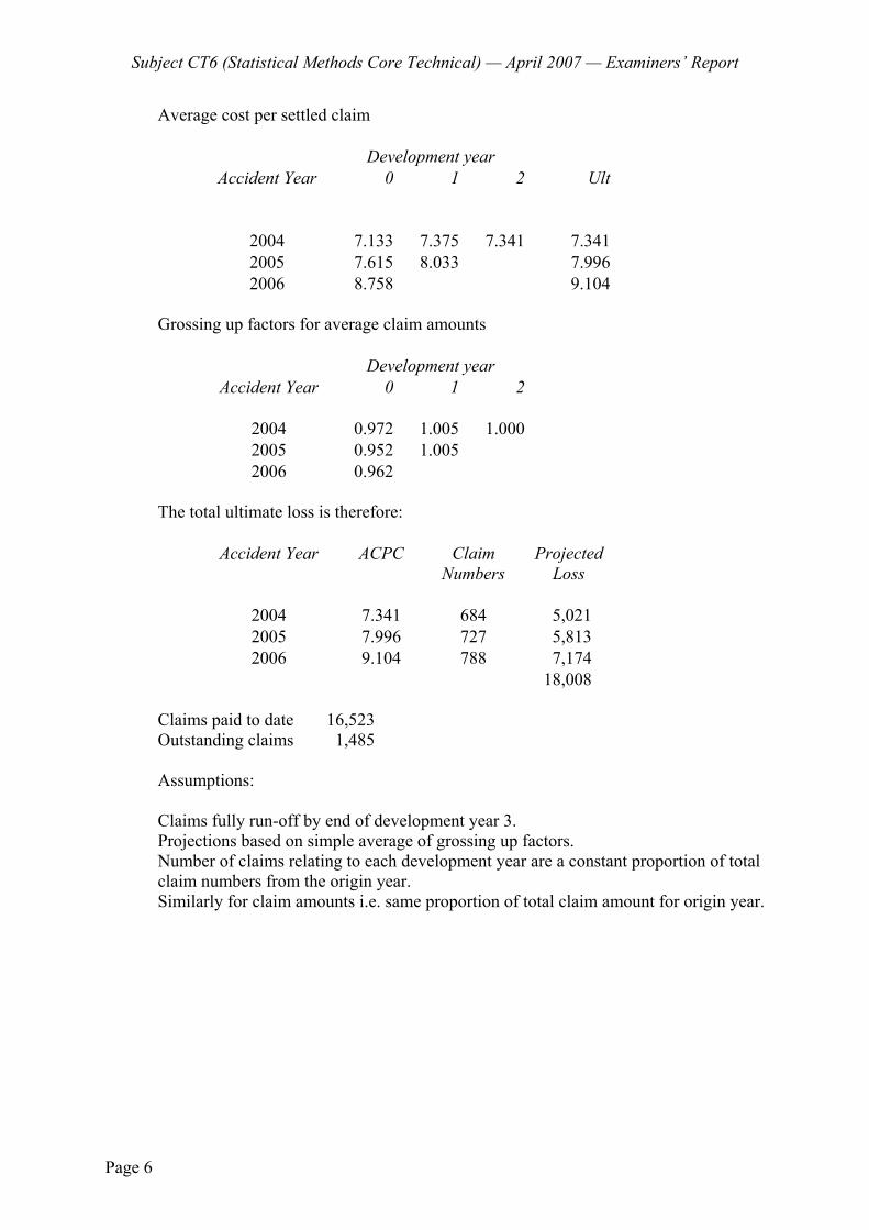
Subject CT6 (Statistical Methods Core Technical) — April 2007 — Examiners’ Report
Page 6
Average cost per settled claim
Development year Accident Year
0 1 2 Ult
2004 7.133 7.375 7.341 7.341 2005 7.615 8.033 7.996 2006 8.758 9.104
Grossing up factors for average claim amounts
Development year
Accident Year
0 1 2
2004 0.972 1.005 1.000 2005 0.952 1.005 2006 0.962
The total ultimate loss is therefore:
Accident Year ACPC Claim Numbers
Projected Loss
2004 7.341 684 5,021 2005 7.996 727 5,813 2006 9.104 788 7,174
18,008 Claims paid to date 16,523 Outstanding claims 1,485
Assumptions: Claims fully run-off by end of development year 3. Projections based on simple average of grossing up factors. Number of claims relating to each development year are a constant proportion of total
claim numbers from the origin year. Similarly for claim amounts i.e. same proportion of total claim amount for origin year.
Subject CT6 (Statistical Methods Core Technical) — April 2007 — Examiners’ Report
Page 7
6 (i) The requirement to calculate cos and sin is time consuming for a computer. The Polar Method avoids this by using the acceptance-rejection method.
(ii) (a) We must transform the values to a log-normal distribution with the
appropriate mean and variance by calculating 5 2ZX e += The required value is 915.1Y X= = = 30.25
(b) We require 2 2
/ 22
zn α τ>
ε
21.645 26.3 71.171×
= =
Hence, 72 simulations are required. 7 1( ) ( ) ( )
1 22 (1 2 )3 310
3
E S E N E X= ×
= × × + ×
=
and I RS S S= + . We will calculate directly the distribution of IS . 2( 0) ( 0) 0.13534IP S P N e−= = = = =
1
21
2 1( 1) ( 1) ( 1) 0.090221! 3IP S P N P X e−= = = = = × =
1 1 21 2
2 2
( 2) ( 1) ( 2) ( 2) ( 1) ( 1)
2 2 2 1 11! 3 2! 3 3
0.21052
IP S P N P X P N P X P X
e e− −
= = = = + = = =
= × + × ×
=
( 3) 1 0.13534 0.09022 0.21052 0.56392IP S = = − − − =
( ) 0 0.13534 1 0.09022 2 0.21052 3 0.563922.20303
IE S = × + × + × + ×=
and hence 10( ) ( ) ( ) ( ) 2.20303 1.1303.3R I IE S E S S E S E S= − = − = − =

Subject CT6 (Statistical Methods Core Technical) — April 2007 — Examiners’ Report
Page 8
8 (i) (a) Magnitude of the residuals increases over time, suggesting that the variance is increasing over time.
More positive than negative residuals suggesting there is drift in the
process. (b) If
iy ( 1,2, ,i n= … ) is a sequence of numbers, it has a turning point at
time k if either 1k ky y− < and 1k ky y +> , or 1k ky y− > and 1k ky y +< . (c) Let T represent the number of turning points, and let N=100 be the
number of data points. Then ( ) 2 / 3( 2) 2 / 3(100 2) 65.333E T N= − = − =
2( ) (16 29) / 90 17.45556 4.178Var T N= − = =
2( 59) ( (65.333, 4.178 ) 59.5)P T P N≥ ≈ >
65.333 59.5( (0,1) ) ( (0,1) 1.396) 0.9194.178
P N P N−= > = > − =
This is a two-sided test so there is approximately a 16% chance of
getting such an extreme number of turning points. This value is not significant at the 5% level, and so this test gives no significant evidence to suggest that the residuals are not a white noise process.
Full credit should also be given for calculating a confidence interval and
checking if 59 is in this. (ii) 100 100 99(1) 5 0.9( 5) 0 0.5 5 0.9(7 5) 0.5 0.7 6.45X X e= + − + + = + − − × = 100 100 100(2) 5 0.9( (1) 5) 0.5 5 0.9(6.45 5) 0.5 1.4 7.005X X e= + − + = + − + × = 100 100 101(3) 5 0.9( (2) 5) 0.5 5 0.9(7.005 5) 6.8045X X e= + − + = + − =

Subject CT6 (Statistical Methods Core Technical) — April 2007 — Examiners’ Report
Page 9
9 (i)
£ Starting level (Year 0) 0% 25% 40%
Year 1 Premium if claim in year 0 1,000 1,000 750 Premium if no claim in year 0 750 600 600 Saving 250 400 150 Year 2 Premium if claim in year 0 750 750 600 Premium if no claim in year 0 600 600 600 Saving 150 150 0 Claim threshold 400 550 150
(ii) P(X > 400) = P(log X > log 400) = P(Z > (log400 - 6)/3.33) = P(Z > -0.0026) = 1 - 0.4990 = 0.5010 P(X > 550) = P(log X > log 550) = P(Z > (log550 - 6)/3.33) = P(Z > 0.0931) = 1 – 0.5371 = 0.4629 P(X > 150) = P(log X > log 150) = P(Z > (log150 - 6)/3.33) = P(Z > -0.2971) = 0.6168 0.12 × 0.5010 = 0.0601 0.12 × 0.4629 = 0.0556 0.12 × 0.6168 = 0.0740 Hence the transition matrix is
0.0601 0.9399 00.0556 0 0.9444
0 0.0740 0.9260
⎡ ⎤⎢ ⎥⎢ ⎥⎢ ⎥⎣ ⎦
(iii) π = π P π0 = 0.0601 π0 + 0.0556 π25 π25 = 0.9399 π0 + 0.0740 π40 π40 = 0.9444 π25+ 0.9260 π40 π25 = 16.905 π0 π40 = 215.740 π0 π0 + π25 + π40 = 1

Subject CT6 (Statistical Methods Core Technical) — April 2007 — Examiners’ Report
Page 10
Hence π = (0.0043, 0.0724, 0.9234) (iv) Stationary distribution if policyholder claims after a loss
0.12 0.88 00.12 0 0.88
0 0.12 0.88P
⎡ ⎤⎢ ⎥= ⎢ ⎥⎢ ⎥⎣ ⎦
π0 = 0.12 π0 + 0.12 π25 π25 = 0.88 π0 + 0.12 π40
π40 = 0.88 π25+ 0.88 π40 π25 = 7.333 π0 π40 = 7.333 π25 = 53.778 π0 π0 + π25 + π40 = 1
Hence:
π = (0.0161, 0.1181, 0.8658)
(v) Award 1 mark for any sensible comment on the reduction in the number of policyholders in the lower discount categories (or increase in the higher discount categories)
10 (i) (a) f(y) = exp log ( 1) log log log ( )y y⎡ ⎤α
− −α μ + α − +α α − Γ α⎢ ⎥μ⎣ ⎦
= exp log ( 1) log log log ( )y y⎡ ⎤⎛ ⎞α − − μ + α − +α α − Γ α⎢ ⎥⎜ ⎟μ⎝ ⎠⎣ ⎦
which is in the form of an exponential family.
θ = 1−μ
b(θ) = log μ
= 1log ⎛ ⎞−⎜ ⎟θ⎝ ⎠ = -log(-θ)

Subject CT6 (Statistical Methods Core Technical) — April 2007 — Examiners’ Report
Page 11
(b) The mean and variance of the distribution are ( )b′ θ and ( ) ( )a b′′ϕ θ
( )b′ θ = 1−θ
= μ
which confirms that the mean is μ.
( )b′′ θ = 21θ
= μ2
a(ϕ) = 1α
hence the variance is 21 ,μα
as required
(ii) A factor is categorical e.g. male/female. For a continuous covariate, the value is included. For example, if x is a
continuous covariate, a main effect would be α + βx. (iii) (a) The linear predictor has the form αi + βj + γx where αi is the factor for policyholder gender (i = 1,2) βj is the factor for vehicle rating group x is the policyholder age (α1 = 0, β1 = 0) (b) The linear predictor becomes αi + βj + γi x

Subject CT6 (Statistical Methods Core Technical) — April 2007 — Examiners’ Report
Page 12
11 (i) (a) The likelihood is given by
1
1
(1 ) (1 )
(1 )
n
n
xx
x x n
L+
∝ θ −θ θ −θ
= θ −θ
and so the log-likelihood is given by 1( ) log log(1 )nl LogL x x n= = + + θ+ −θ and differentiating gives
11
nx xdl nd
+ += −
θ θ −θ
setting this expression to zero to find the maximum gives
1
1
1 1
1
1
0ˆ ˆ1ˆ ˆ( )(1 )
ˆ( ) ( )
ˆ
n
n
n n
n
n
x x n
x x n
x x n x xx x
n x x
+ +− =
θ −θ+ + −θ = θ
+ + = + + + θ
+ +θ =
+ + +
to check this is a maximum, note that
2
12 2 2 0
(1 )nx xd l n
d+ +
= − − <θ θ −θ
(b) The posterior distribution is given by
1
1
1 1
1 1
( ) ( ) ( )
(1 ) (1 )
(1 )
n
n
x x n
x x n
f x g x f+ + α− α−
α+ + + − +α−
θ ∝ θ θ
= θ −θ ×θ −θ
= θ −θ
which is the pdf of a beta distribution with parameters 1 nx xα + + +
and nα + . (c) First note that the prior distribution of θ is Beta with parameters α
and α . Hence its mean is
1/ 2α=
α +α.

Subject CT6 (Statistical Methods Core Technical) — April 2007 — Examiners’ Report
Page 13
Under Bayesian loss, the estimator is given by the mean of the posterior distribution, which is
* 2 1
2 2 2 2ˆ (1 )
i i i
i i i i
x x x nx n x n x n x n
Z Z
α + + αθ = = × + ×
α + + + α + + α + +
= θ× + − μ
∑ ∑ ∑∑ ∑ ∑ ∑
Where 2
i
i
x nZ
x n+
=α + +∑∑
and 1/ 2μ = is the prior mean of θ .
(d) As n increases, Z tends towards 1, and the Bayes estimate approaches
the maximum likelihood estimate, as more credibility is put on the data, and less on the prior estimate.
(ii) (a) The variance of the prior distribution is given by:
2
21
4(2 1)(2 ) (2 1)α
=α +α α +
.
(b) Higher values of α result in a lower variance and hence imply greater
certainty over the prior value of θ . In the special case where 1α = the prior distribution is Uniform on
[0,1] implying that we have no particular reason to believe that any prior value of θ is more or less likely than any other.
(iii) 3 3 5 11ix = + + =∑
(a) * 5 11 16 2 0.66672 5 11 3 24 3
+θ = = = =
× + +
(b) * 2 11 13 0.72222 2 11 3 18
+θ = = =
× + +
The first set of parameters has greater certainty attached to the prior estimate
(i.e. a higher value of α ), and therefore the posterior estimate is closer to the mean of the prior distribution (which is 0.5) than in the second case.
END OF MARKING SCHEDULE

Faculty of Actuaries Institute of Actuaries
EXAMINATION
2 October 2007 (am)
Subject CT6 — Statistical Methods Core Technical
Time allowed: Three hours
INSTRUCTIONS TO THE CANDIDATE
1. Enter all the candidate and examination details as requested on the front of your answer booklet.
2. You must not start writing your answers in the booklet until instructed to do so by the
supervisor. 3. Mark allocations are shown in brackets. 4. Attempt all 10 questions, beginning your answer to each question on a separate sheet. 5. Candidates should show calculations where this is appropriate.
Graph paper is not required for this paper.
AT THE END OF THE EXAMINATION
Hand in BOTH your answer booklet, with any additional sheets firmly attached, and this question paper.
In addition to this paper you should have available the 2002 edition of the Formulae and Tables and your own electronic calculator.
© Faculty of Actuaries CT6 S2007 © Institute of Actuaries
CT6 S2007—2
1 An investment actuary notices that the volatility of the price of a particular asset is much higher following a significant change in the price of the asset.
Define an ARCH model and explain what particular properties of the model would
make it appropriate for modelling this asset. [5] 2 Two poachers can escape from either the farmyard or the fields of an estate. Two
gamekeepers are employed by the estate to catch them. The gamekeepers have three options: both patrol the farmyard (action a1); one of them patrols the farmyard and the other patrols the fields (action a2); both gamekeepers patrol the fields (action a3). The poachers also have three options: both try to escape through the farmyard (option θ1); one of them tries to escape from the farmyard and the other from the fields (option θ2); both try to escape over the fields (option θ3). The number of birds they manage to poach under each combination of θi and aj can be found in the following table:
a1 a2 a3 θ1 0 90 120 θ2 75 0 75 θ3 120 90 0
Assume the goal of the gamekeepers and the poachers is to minimise and maximise
the number of birds poached, respectively. (i) Show that θ1 does not dominate θ2 and vice versa. [1] (ii) Determine the minimax solution to this problem for the gamekeepers, and
state the maximum number of birds that will be poached if they adopt this strategy. [2]
(iii) Given the prior distribution P(θ1) = 0.25, P(θ2) = 0.35 and P(θ2) = 0.4,
determine the Bayes solution to the problem for the gamekeepers. [3] [Total 6] 3 The number of claims, N, in a year on a portfolio of insurance policies has a Poisson
distribution with parameter λ. Claims are either large (with probability p) or small (with probability 1 - p) independently of one another.
Suppose we observe r large claims. Show that the conditional distribution of |N r r−
is Poisson and find its mean. [7]
CT6 S2007—3 PLEASE TURN OVER
4 The table below gives the cumulative incurred claims by year and earned premiums for a particular type of motor policy (Figures in £000s).
Claims paid to date total £15,000,000. The ultimate loss ratio is expected to be in line
with the 2003 accident year.
Development year Accident
Year
0 1 2 3 Earned Premiums
2003 3,340 3,750 4,270 4,400 4,800 2004 3,670 4,080 4,590 4,900 2005 3,690 4,290 5,050 2006 4,150 5,200
Ignoring inflation, use the Bornhuetter-Ferguson method to calculate the total reserve
required to meet the outstanding claims, assuming that the claims are fully developed by the end of development year 3. [8]
5 Aggregate annual claims on a portfolio of insurance policies have a compound
Poisson distribution with parameter λ. Individual claim amounts have an exponential distribution with mean 1.
The insurer calculates premiums using a loading of α (so that the annual premium is
1+α times the annual expected claims) and has initial surplus U. (i) Show that if the first claim occurs at time t, the probability that this claim
causes ruin is (1 )U te e− − +α λ . [3]
(ii) Show that the probability of ruin on the first claim is 2
Ue−
+ α. [4]
(iii) Show that if the insurer wishes to set α such that the probability of ruin at the
first claim is less than 1% then it must choose 100 2Ue−α > − . [2] [Total 9]
CT6 S2007—4
6 Claim sizes (in suitable units) for a portfolio of insurance policies come from a distribution with probability density function
2
0 2 0( )0 otherwise
xaxe x af x−⎧⎪ ≤ ≤ >= ⎨
⎪⎩
where a > 0 is a constant. (i) Find a. [2] (ii) Show that ( ) 1f x ≤ . [2] (iii) Random numbers have been drawn from a U(0,1) distribution, and are
arranged in pairs. The first three pairs are:
0.7413 and 0.4601 0.3210 and 0.6316
0.5069 and 0.0392 Using the rectangle { }( , ) 0 2, 0 1x y x y≤ ≤ ≤ ≤ and the pairs of random
numbers in the order given above, use the acceptance-rejection method to generate a single observation from the claim size distribution. [3]
(iv) Estimate the average number of U(0,1) variables needed to generate a
simulation using the approach in (iii). [1] (v) The results of many thousands of simulations generated in this way are to be
used to compare the impact of two possible reinsurance treaties on the insurer’s profitability. Explain, with a reason, whether the modeller should use the same simulated claims for each treaty in his model, or whether a new sample for each treaty should be generated. [2]
[Total 10]

CT6 S2007—5 PLEASE TURN OVER
7 A no claims discount system has 4 levels. The premiums paid by policyholders in each level are as follows:
Level Premium 0 100% 25 75% 40 60% 50 50% The rules for moving between the levels are as follows:
• following a claim-free year, a policyholder moves to the next higher level of discount, or remains at 50% discount
• following a year of one or more claims, a policyholder moves to the next lower
discount rate or remains at 0% discount It is assumed that claims occur according to a Poisson process with rate λ per year per
policyholder, and that the equilibrium distribution has been reached.
(i) Show that the average premium paid, if the premium paid by a policyholder in level 0 is £500, may be written as
2 3
2 31 0.75 0.6 0.5500
1k k kk k k
⎛ ⎞+ + +⎜ ⎟⎜ ⎟+ + +⎝ ⎠
where k = 1
ee
−λ
−λ− [5]
(ii) Calculate the average premium paid by policyholders whose claim rate per
year is (a) 0.12, (b) 0.24, (c) 0.36. [3] (iii) Comment on the results in (ii), in relation to the effectiveness of the no claims
discount system discriminating between good and bad drivers. [2] [Total 10]
CT6 S2007—6
8 The total claim amount, S, on a portfolio of insurance policies has a compound Poisson distribution with Poisson parameter 50. Individual loss amounts have an exponential distribution with mean 75. However, the terms of the policies mean that the maximum sum payable by the insurer in respect of a single claim is 100.
(i) Find E(S) and Var (S). [7] (ii) Use the method of moments to fit as an approximation to S: (a) a normal distribution (b) a log-normal distribution [3] (iii) For each fitted distribution, calculate P(S > 3,000). [3] [Total 13] 9 y1, y2, …, yn are independent, identically distributed observations with probability
function given by ( )|!
iy
ii
ef yy
−μμμ = .
(i) Show that the log-likelihood may be written as
( )1
n
ii
y nb=
θ − θ +∑ terms not depending on θ
and identify the natural parameter, θ , and the function ( )b θ . [3]
(ii) The fitted value for observation yi is denoted by ˆ .iy
(a) Write down the Pearson residual for yi, in terms of yi and ˆ .iy (b) Explain why Pearson residuals are usually not suitable for model
checking for the Poisson distribution. [3]
(iii) Show that the conjugate prior density function forθ is proportional to
{ }exp eθαθ−β , and derive the posterior distribution for this prior. [4]
(iv) Use the identity log 0fE ∂⎡ ⎤ =⎢ ⎥∂θ⎣ ⎦ (for any density function f) to show that
( )E b α⎡ ⎤θ =⎣ ⎦ β
and ( ) 11 2| , , ,
n
ii
n
yE b y y y
n=
α +⎡ ⎤θ =⎣ ⎦ β +
∑… , and comment on these
results. [5] [Total 15]
CT6 S2007—7
10 The time series tX is assumed to be stationary and to follow an ARMA (2,1) process defined by:
tX = 1 + 815
1tX − – 115
2tX − + tΖ – 17 1t−Ζ
where Zt are independent N(0,1) random variables. (i) Determine the roots of the characteristic polynomial, and explain how their
values relate to the stationarity of the process. [2] (ii) (a) Find the autocorrelation function for lags 0, 1 and 2. (b) Derive the autocorrelation at lag k in the form
ρk = kAc
+ kB
d
[12] (iii) Determine the mean and variance of Xt. [3] [Total 17]
END OF PAPER
Faculty of Actuaries Institute of Actuaries
EXAMINATION
September 2007
Subject CT6 — Statistical Methods Core Technical
EXAMINERS’ REPORT
Introduction The attached subject report has been written by the Principal Examiner with the aim of helping candidates. The questions and comments are based around Core Reading as the interpretation of the syllabus to which the examiners are working. They have however given credit for any alternative approach or interpretation which they consider to be reasonable. M A Stocker Chairman of the Board of Examiners December 2007
© Faculty of Actuaries © Institute of Actuaries

Subject CT6 (Statistical Methods Core Technical) — September 2007 — Examiners’ Report
Page 2
Comments Overall it is clear that candidates found this a tougher paper than in other recent sittings. In particular, candidates who did not have a firm grasp of the basic statistical material covered in subject CT3 struggled with some of the questions.
Comments on individual questions are as follows: Q1 The Examiners had intended this to be a straightforward bookwork question as it is
taken largely verbatim from the core reading. However, very few candidates could recall this part of the core reading accurately and therefore most candidates struggled to score any marks.
Q2 Well answered. There was a minor typographical error in the question, but virtually
all candidates seemed to have understood what was intended. The Examiners allowed any alternative interpretation provided it was clearly stated.
Q3 In general, this question was very poorly answered. Most candidates appeared
unable to apply Bayes’ Theorem to the situation given in the question. Q4 Well answered. Q5 Parts (i) and (iii) were generally well answered, a pleasing improvement relative to
similar questions from recent sittings. Only the better candidates were able to complete part (ii).
Q6 This was the first time in a number of sittings that this material has been tested. Most
of the better candidates coped reasonably well with parts (i), (ii) and (v). Weaker candidates struggled badly with (i) and (ii) which required only some calculus. Part (iii) was actually simpler than many candidates appear to have expected and as a result many solutions were over-complicated and scored poorly.
Q7 Well answered. Q8 This question was well answered by the better candidates. Many candidates picked
up significant follow through marks in parts (ii) and (iii) despite making numerical errors in part (i).
Q9 Part (i) was generally well answered. The remaining parts were tougher, with a
number of candidates quoting the results in parts (iii) and (iv) rather than deriving them as instructed.
Q10 Parts (i) and (iii) were well answered. Most candidates were able to make some
progress with (ii) (a) though a number struggled to derive three correct equations. Only the best candidates were able to answer (ii) (b).
Subject CT6 (Statistical Methods Core Technical) — September 2007 — Examiners’ Report
Page 3
1 An ARCH(p) model is
Xt = μ + 20
1( )
p
t k t kk
e X −=
α + α −μ∑
where et are independent N(0,1). Often, this is used to model ln(Zt/Zt-1) where Zt is the asset price. It can be seen that a large departure in Xt-k from μ will result in Xt having a larger
variance. This will then result in a large volatility for the asset price. 2 (i) θ1 would dominate θ2 (and vice versa) if the amount of birds poached under
each of a1, a2 and a3 is higher in each case for θ1 (θ2) θ1 provides a better outcome for a2 (90 > 0) and a3 (120 > 75) θ2 provides a better outcome for a1 (0 < 75) (ii) Minimax solution for gamekeepers. Worst loss under each option would be: a1 = max (0,75,120) = 120 a2 = max (90,0,90) = 90 a3 = max (120,75,0) = 120 Therefore, gamekeepers would choose a2 and lose 90 birds. (iii) a1 = 0.25 × 0 + 0.35 × 75 + 0.4 × 120 = 74.25 a2 = 0.25 × 90 + 0.35 × 0 + 0.4 × 90 = 58.5 a3 = 0.25 × 120 + 0.35 × 75 + 0.4 × 0 = 56.25 Hence the Bayes decision is a3.
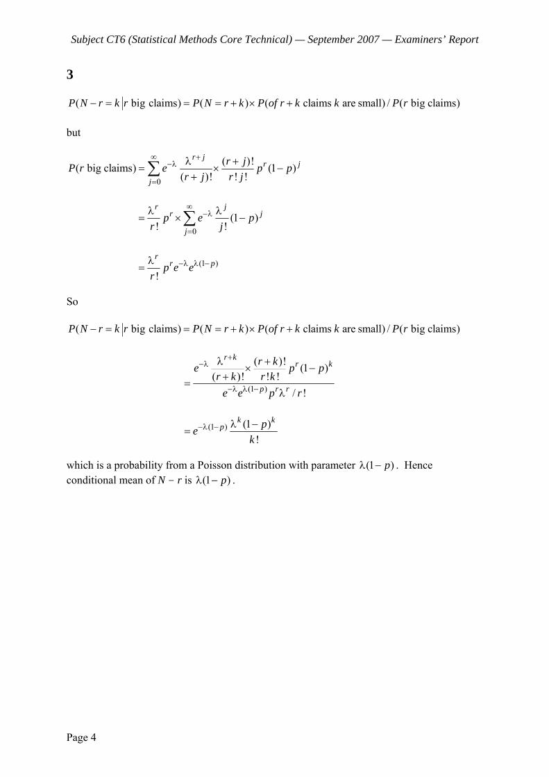
Subject CT6 (Statistical Methods Core Technical) — September 2007 — Examiners’ Report
Page 4
3
( big claims) ( ) ( claims are small) / ( big claims)P N r k r P N r k P of r k k P r− = = = + × + but
0
( )!( big claims) (1 )( )! ! !
r jr j
j
r jP r e p pr j r j
∞ +−λ
=
λ += × −
+∑
0
(1 )! !
r jr j
jp e p
r j
∞−λ
=
λ λ= × −∑
(1 )!
rr pp e e
r−λ λ −λ
=
So
( big claims) ( ) ( claims are small) / ( big claims)P N r k r P N r k P of r k k P r− = = = + × +
(1 )
( )! (1 )( )! ! !
/ !
r kr k
p r r
r ke p pr k r k
e e p r
+−λ
−λ λ −
λ +× −+=
λ
(1 ) (1 )!
k kp pe
k−λ − λ −
=
which is a probability from a Poisson distribution with parameter (1 )pλ − . Hence conditional mean of N - r is (1 )pλ − .

Subject CT6 (Statistical Methods Core Technical) — September 2007 — Examiners’ Report
Page 5
4 The development factors are:
Development year Accident
Year
0 1 2 3 EP
2003 3,340 3,750 4,270 4,400 4,800 2004 3,670 4,080 4,590 4,900 2005 3,690 4,290 5,050 2006 4,150 5,200 10,700 7,830 4,270 12,120 8,860 4,400 Development factors 1.1327 1.1315 1.0304 Cumulative DFs 1.3207 1.1660 1.0304 Ultimate loss ratio 4,400/4,800 = 0.9167
Estimated ultimate loss for each accident year: Accident
Year ULR EP UL Expected
claimsClaims to be
incurred
2003 0.9167 4,800 4,400 4,400 0 2004 0.9167 4,900 4,492 4,359 133 2005 0.9167 5,050 4,629 3,970 659 2006 0.9167 5,200 4,767 3,609 1,158
Revised ultimate losses are: Accident
Year Claims
incurred Claims to be
incurredRevised UL
2003 4,400 0 4,400 2004 4,590 133 4,723 2005 4,290 659 4,949 2006 4,150 1,158 5,308 19,379 Claims to date 15,000 Reserve required 4,379

Subject CT6 (Statistical Methods Core Technical) — September 2007 — Examiners’ Report
Page 6
5 (i) Let X be the size of the first claim, so that X has an exponential distribution with parameter 1. Then for ruin to occur at time t we require
X > U + (1 + α) λt.
P(X > U + (1 + α) λt) = (1 )
x
U t
e dx∞
−
+ +α λ∫
= (1 )
xU t
e∞−+ +α λ
⎡ ⎤−⎣ ⎦
= e-Ue-(1+α)λt.
[Note that it would be acceptable to quote the cumulative distribution function for the exponential distribution from the tables rather than calculate the integral]
(ii) Let T denote the time until the first claim. Then T has an exponential
distribution with parameter λ and
P(Ruin at first claim) = 0
(Ruin at first claim first claim is at ) ( )TP t f t dt∞
⏐ ×∫
= ∫∞
−+−−
0
)1( dteee ttU λλα λ
= (2 )
0
U te e dt∞
− − +α λλ∫
= (2 )
0(2 )U te e
∞− − +α λ⎡ ⎤λ
−⎢ ⎥+ α λ⎣ ⎦
= .2
Ue−
+ α

Subject CT6 (Statistical Methods Core Technical) — September 2007 — Examiners’ Report
Page 7
(iii) We require
0.012
Ue−<
+α
i.e. e-U < 0.01 × (2 + α) i.e. 100e-U < 2 + α. i.e. 100e-U – 2 < α.
6 (i) We find a by solving:
2
0
( ) 1f x dx =∫
2
2
0
1xaxe dx− =∫
2
2
01
2xa e−⎡ ⎤− =⎢ ⎥⎣ ⎦
4( 1) 12a e−−
− =
42 2.03731
1a
e−−
= =−
(ii) We find the local maximum value of f(x) by differentiation:
2 2 22 2'( ) 2 (1 2 )x x xf x ae ax e ae x− − −= − = −
and this derivative is zero when
22 1
0.70711x
x=
= ±
and f(0.70711) = 0.8738.
Note that f(0) = 0 and f(2) = 0.07463 so that the maximum value on [0,2] is 0.8738 and so ( ) 1f x < as required.
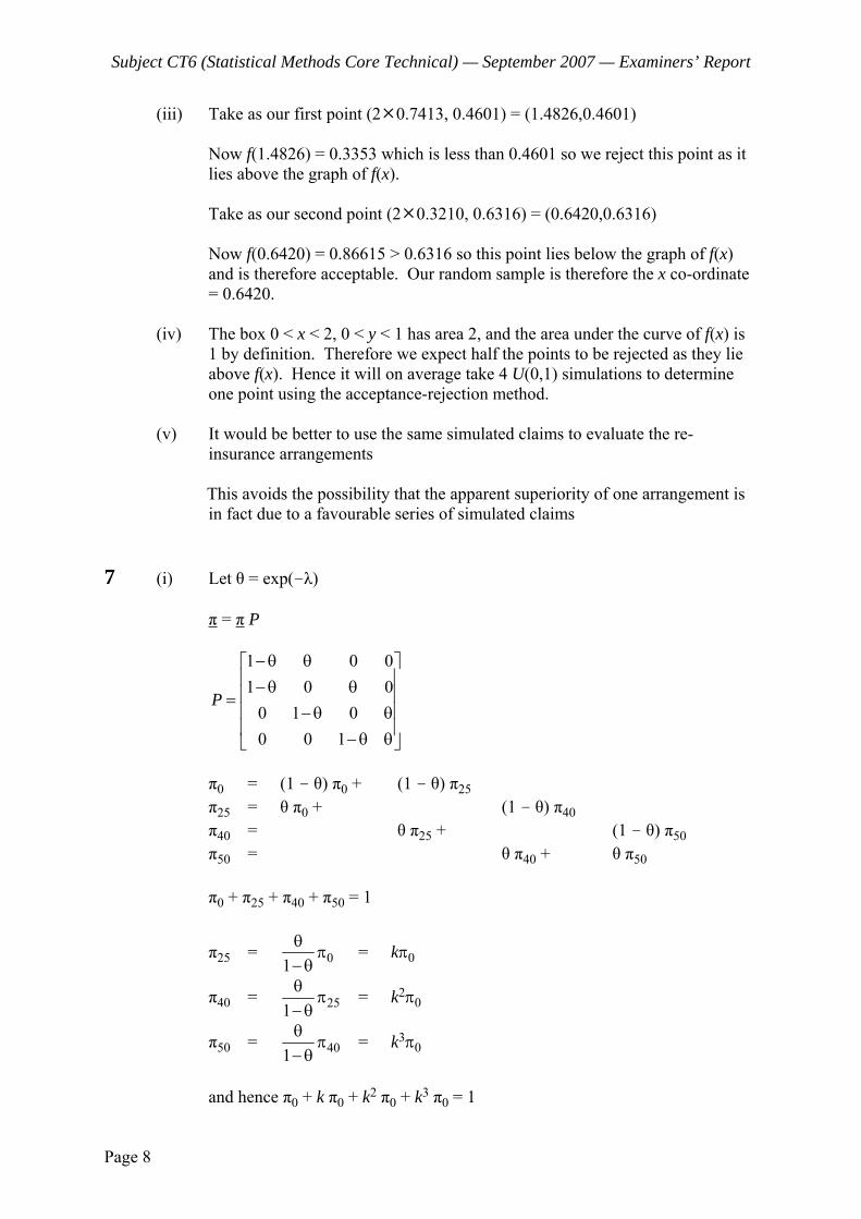
Subject CT6 (Statistical Methods Core Technical) — September 2007 — Examiners’ Report
Page 8
(iii) Take as our first point (2 0.7413, 0.4601) = (1.4826,0.4601) Now f(1.4826) = 0.3353 which is less than 0.4601 so we reject this point as it
lies above the graph of f(x). Take as our second point (2 0.3210, 0.6316) = (0.6420,0.6316) Now f(0.6420) = 0.86615 > 0.6316 so this point lies below the graph of f(x)
and is therefore acceptable. Our random sample is therefore the x co-ordinate = 0.6420.
(iv) The box 0 < x < 2, 0 < y < 1 has area 2, and the area under the curve of f(x) is
1 by definition. Therefore we expect half the points to be rejected as they lie above f(x). Hence it will on average take 4 U(0,1) simulations to determine one point using the acceptance-rejection method.
(v) It would be better to use the same simulated claims to evaluate the re-
insurance arrangements
This avoids the possibility that the apparent superiority of one arrangement is in fact due to a favourable series of simulated claims
7 (i) Let θ = exp(-λ) π = π P
1 0 01 0 0
0 1 00 0 1
P
−θ θ⎡ ⎤⎢ ⎥− θ θ⎢ ⎥=⎢ ⎥− θ θ⎢ ⎥− θ θ⎣ ⎦
π0 = (1 - θ) π0 + (1 - θ) π25 π25 = θ π0 + (1 - θ) π40 π40
= θ π25 + (1 - θ) π50 π50 = θ π40 + θ π50
π0 + π25 + π40 + π50 = 1
π25 = 01θ
π−θ
= kπ0
π40 = 251θ
π−θ
= k2π0
π50 = 401θ
π−θ
= k3π0
and hence π0 + k π0 + k2 π0 + k3 π0 = 1
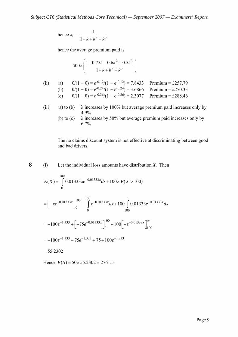
Subject CT6 (Statistical Methods Core Technical) — September 2007 — Examiners’ Report
Page 9
hence π0 = 2 31
1 k k k+ + +
hence the average premium paid is
2 3
2 31 0.75 0.6 0.5500
1k k kk k k
⎛ ⎞+ + +×⎜ ⎟⎜ ⎟+ + +⎝ ⎠
(ii) (a) θ/(1 - θ) = e-0.12/(1 – e-0.12) = 7.8433 Premium = £257.79 (b) θ/(1 - θ) = e-0.24/(1 – e-0.24) = 3.6866 Premium = £270.33 (c) θ/(1 - θ) = e-0.36/(1 – e-0.36) = 2.3077 Premium = £288.46 (iii) (a) to (b) λ increases by 100% but average premium paid increases only by
4.9% (b) to (c) λ increases by 50% but average premium paid increases only by
6.7%
The no claims discount system is not effective at discriminating between good
and bad drivers. 8 (i) Let the individual loss amounts have distribution X. Then
100
0.01333
0
( ) 0.01333 100 ( 100)xE X xe dx P X−= + × >∫
1001000.01333 0.01333 0.01333
00 100
100 0.01333x x xxe e dx e dx∞
− − −⎡ ⎤= − + +⎣ ⎦ ∫ ∫
1001.333 0.01333 0.013330 100
100 75 100x xe e e∞− − −⎡ ⎤ ⎡ ⎤= − + − + −⎣ ⎦ ⎣ ⎦
1.333 1.333 1.333100 75 75 100e e e− − −= − − + + 55.2302= Hence ( ) 50 55.2302 2761.5E S = × =

Subject CT6 (Statistical Methods Core Technical) — September 2007 — Examiners’ Report
Page 10
100
2 2 0.01333 2
0
( ) 0.01333 100 ( 100)xE X x e dx P X−= + >∫
1001002 0.01333 0.01333 2 1.333
00
2 100x xx e xe dx e− − −⎡ ⎤= − + +⎣ ⎦ ∫
1001002 1.333 0.01333 0.01333 2 1.333
0 0
2 2100 1000.01333 0.01333
x xxe e e dx e− − − −⎡ ⎤= − + − + +⎢ ⎥⎣ ⎦ ∫
100
1.333 0.013332
0
200 20.01333 0.01333
xe e− −⎡ ⎤= − + −⎢ ⎥⎣ ⎦
1.333 1.3332 2
200 2 20.01333 0.01333 0.01333
e e− −= − − +
4330.6= and so 2( ) 50 4330.6 216529 (465.33)Var S = × = = (ii) (a) The normal distribution is N(2761.5, 465.332) (b) The Log-Normal distribution has parameters and μ σ with
2
2 2 2
/ 2
2 2
( )
( ) ( 1) ( ) ( 1)
E S e
Var S e e E S e
μ+σ
μ+σ σ σ
=
= − = × −
So substituting gives
22216529 2761.5 ( 1)eσ= × −
2
2216529 1 1.0283942761.5
eσ = + =
2 log(1.028394) 0.027998σ = = 0.167327σ = And now we can substitute for σ to give
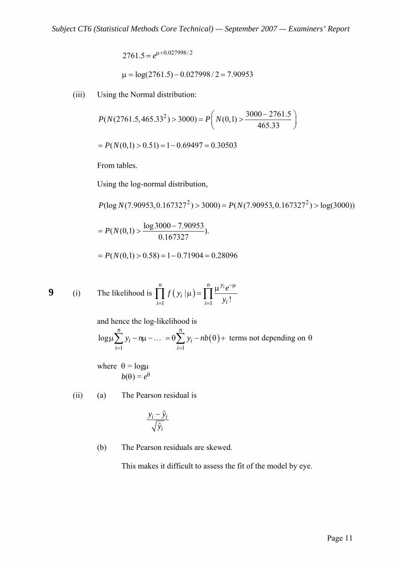
Subject CT6 (Statistical Methods Core Technical) — September 2007 — Examiners’ Report
Page 11
0.027998/ 22761.5 eμ+= log(2761.5) 0.027998 / 2 7.90953μ = − = (iii) Using the Normal distribution:
2 3000 2761.5( (2761.5,465.33 ) 3000) (0,1)465.33
P N P N −⎛ ⎞> = >⎜ ⎟⎝ ⎠
( (0,1) 0.51) 1 0.69497 0.30503P N= > = − = From tables. Using the log-normal distribution, 2 2(log (7.90953,0.167327 ) 3000) ( (7.90953,0.167327 ) log(3000))P N P N> = >
log3000 7.90953( (0,1) ).0.167327
P N −= >
( (0,1) 0.58) 1 0.71904 0.28096P N= > = − =
9 (i) The likelihood is ( )1 1
|!
in n y
iii i
ef yy
−μ
= =
μμ =∏ ∏
and hence the log-likelihood is
1
logn
ii
y n=
μ − μ −∑ … ( )1
n
ii
y nb=
= θ − θ +∑ terms not depending on θ
where θ = logμ b(θ) = eθ (ii) (a) The Pearson residual is
ˆ
ˆi i
i
y yy−
(b) The Pearson residuals are skewed. This makes it difficult to assess the fit of the model by eye.
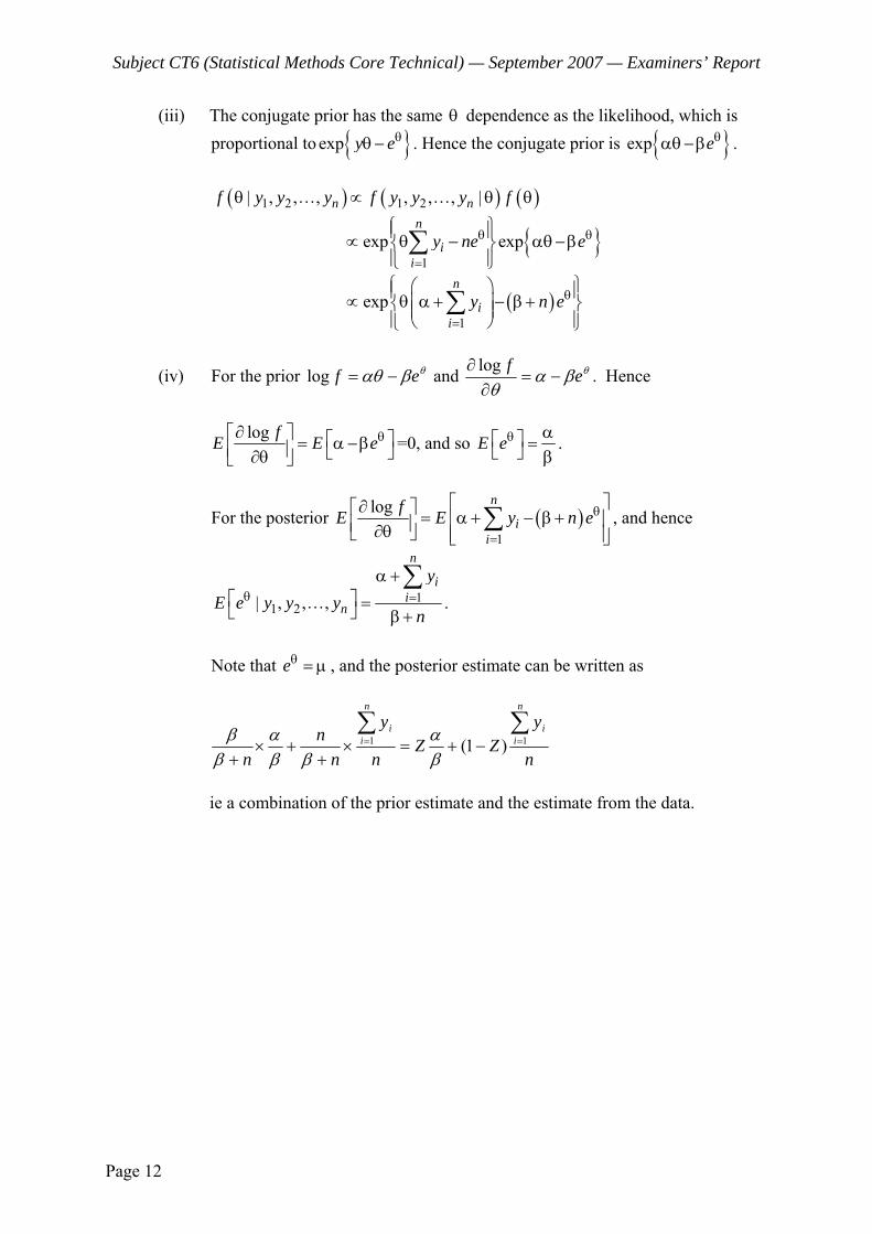
Subject CT6 (Statistical Methods Core Technical) — September 2007 — Examiners’ Report
Page 12
(iii) The conjugate prior has the same θ dependence as the likelihood, which is proportional to { }exp y eθθ − . Hence the conjugate prior is { }exp eθαθ−β .
( ) ( ) ( )1 2 1 2| , , , , , , |n nf y y y f y y y fθ ∝ θ θ… …
{ }1
exp expn
ii
y ne eθ θ
=
⎧ ⎫⎪ ⎪∝ θ − αθ−β⎨ ⎬⎪ ⎪⎩ ⎭∑
( )1
expn
ii
y n eθ=
⎧ ⎫⎛ ⎞⎪ ⎪∝ θ α + − β+⎜ ⎟⎨ ⎬⎜ ⎟⎪ ⎪⎝ ⎠⎩ ⎭∑
(iv) For the prior θβαθ ef −=log and θβαθ
ef−=
∂∂ log . Hence
log fE E eθ∂⎡ ⎤ ⎡ ⎤= α −β⎢ ⎥ ⎣ ⎦∂θ⎣ ⎦
=0, and so E eθ α⎡ ⎤ =⎣ ⎦ β.
For the posterior ( )1
log n
ii
fE E y n eθ=
⎡ ⎤∂⎡ ⎤ = α + − β+⎢ ⎥⎢ ⎥∂θ⎣ ⎦ ⎢ ⎥⎣ ⎦∑ , and hence
11 2| , , ,
n
ii
n
yE e y y y
nθ =
α +⎡ ⎤ =⎣ ⎦ β+
∑… .
Note that eθ = μ , and the posterior estimate can be written as
n
yZZ
n
y
nn
n
n
ii
n
ii ∑∑
== −+=×+
+×+
11 )1(βα
ββα
ββ
ie a combination of the prior estimate and the estimate from the data.

Subject CT6 (Statistical Methods Core Technical) — September 2007 — Examiners’ Report
Page 13
10 (i) The characteristic equation is given by:
(1 - 815
λ + 115
2λ ) = (1 - 13
λ ) (1 - 15λ ) = 0
which has roots = 3 and 5. They are both greater than 1. Hence, subject to the
initial values having appropriate distributions, this implies (weak) stationarity. (ii) (a)
Firstly, note that 1),( =tt ZXCov and 105/417/115/8),( 1 =−=−tt ZXCov We need to generate 3 distinct equations linking 0γ , 1γ and 2γ This can be done as follows: (A)
735/69415/115/8105/417/1115/115/8
),7/115/115/81(),(
21
21
1210
+−=×−+−=
−+−+== −−−
γγγγ
γ ttttttt XZZXXCovXXCov
(B)
7/115/115/8),7/115/115/81(),(
10
112111
−−=−+−+== −−−−−
γγγ ttttttt XZZXXCovXXCov
(C)
01
212122
15/115/8),7/115/115/81(),(
γγγ
−=−+−+== −−−−− ttttttt XZZXXCovXXCov
Next stage is to solve these equations. Substituting (C) into (A) gives
5488/5205)2/1(735/694)225/112()225/224(
735/694))15/1()15/8)((15/1()15/8(
10
10
0110
+=+=
+−−=
γγγγ
γγγγso
Subject CT6 (Statistical Methods Core Technical) — September 2007 — Examiners’ Report
Page 14
Now substituting into (B) gives
4537.02744/1245686/249)5/4(
7/1)15/1()5488/5205)2/1((15/8
1
1
111
===
−−+=
γγ
γγγso
And
1636.01753.115/14537.015/81753.15488/52054537.02/1
2
0
=×−×==+×=
γγ
Finally,
0ρ = 1, 1ρ = 1
0
γγ
= 0.386, 2ρ = 2
0
γγ
= 0.139
(b) kρ = 815
1k−ρ - 115
2k−ρ for k ≥ 2
We will show that the solution has the form:
kρ = A ( 13
)k + B ( 15
)k
Substituting the proposed solution into the recurrence relation gives
815
1k−ρ - 115
2k−ρ = 815
[ A ( 12
)k-1 + B ( 15
)k–1] - 115
[ A ( 13
)k–2 + B ( 15
)k–2]
= A ( 13
)k ( 815
× 3 - 15
× 9) + B ( 15
)k ( 815
× 5 - 115
× 25)
= A ( 13
)k + B ( 15
)k
= kρ
So the solution does have this form.

Subject CT6 (Statistical Methods Core Technical) — September 2007 — Examiners’ Report
Page 15
The values of A and B are fixed by 0ρ = 1, 1ρ = 0.386 ∴ A + B = 1
13
A + 15
B = 0.386
→ 13
A + 15
(1 – A ) = 0.386
A = 1.395 B = -0.395
∴ kP = 1.395 ( 13
)k – 0.395 ( 15
)k
(iii) We require mean and variance of tX which must be normally distributed
since Z is normally distributed. Variance is 0γ = 1.1753 from (ii) (a)
E ( tX ) = 1 + 815
E ( tX ) - 115
E ( tX )
∴E ( tX ) = 158
END OF EXAMINERS’ REPORT

Faculty of Actuaries Institute of Actuaries
EXAMINATION
8 April 2008 (am)
Subject CT6 — Statistical Methods Core Technical
Time allowed: Three hours
INSTRUCTIONS TO THE CANDIDATE
1. Enter all the candidate and examination details as requested on the front of your answer booklet.
2. You must not start writing your answers in the booklet until instructed to do so by the
supervisor. 3. Mark allocations are shown in brackets. 4. Attempt all 10 questions, beginning your answer to each question on a separate sheet. 5. Candidates should show calculations where this is appropriate.
Graph paper is not required for this paper.
AT THE END OF THE EXAMINATION
Hand in BOTH your answer booklet, with any additional sheets firmly attached, and this question paper.
In addition to this paper you should have available the 2002 edition of the Formulae and Tables and your own electronic calculator from the approved list.
© Faculty of Actuaries CT6 A2008 © Institute of Actuaries

CT6 A2008—2
1 Give two examples of the main types of liability insurance, stating for each example a typical insured peril. [4]
2 A claim amount distribution is normal with unknown mean μ and known standard
deviation £50. Based on past experience a suitable prior distribution for μ is normal with mean £300 and standard deviation £20.
(i) Calculate the prior probability that μ, the mean of the claim amount
distribution, is less than £270. [1]
(ii) A random sample of 10 current claims has a mean of £270.
(a) Determine the posterior distribution of μ. (b) Calculate the posterior probability that μ is less than £270 and
comment on your answer. [5] [Total 6] 3 (i) X and Y are independent Poisson random variables with mean λ. Derive the
moment generating function of X, and hence show that X + Y also has a Poisson distribution. [4]
(ii) An insurer has a portfolio of 100 policies. Annual premiums of 0.2 units per
policy are payable annually in advance. Claims, which are paid at the end of the year, are for a fixed sum of 1 unit per claim. Annual claims numbers on each policy are Poisson distributed with mean 0.18.
Calculate how much initial capital is needed in order to ensure that the
probability of ruin at the end of the year is less than 1%. [4] [Total 8] 4 Y1, Y2, …, Yn are independent observations from a normal distribution with E[Yi] = μi
and Var[Yi] = σ2. (i) Write the density of Yi in the form of an exponential family of distributions. [2] (ii) Identify the natural parameter and derive the variance function. [3] (iii) Show that the Pearson residual is the same as the deviance residual. [4] [Total 9]
CT6 A2008—3 PLEASE TURN OVER
5 The following table shows the claim payments for an insurance company in units of £5,000:
Development year
Accident year
0 1 2 3
2004 410 814 216 79 2005 575 940 281 2006 814 1066 2007 1142
The inflation for a 12 month period to the middle of each year is given as follows:
2005 2006 20075% 5.5% 5.4%
The future inflation from 2007 is estimated to be 8% per annum. Claims are fully run-off at the end of the development year 3. Calculate the amount of outstanding claims arising from accidents in year 2007, using
the inflation adjusted chain ladder method. [9] 6 A portfolio of general insurance policies is made up of two types of policies. The
policies are assumed to be independent, and claims are assumed to occur according to a Poisson process. The claim severities are assumed to have exponential distributions.
For the first type of policy, a total of 65 claims are expected each year and the
expected size of each claim is £1,200. For the second type of policy, a total of 20 claims are expected each year and the
expected size of each claim is £4,500. (i) Calculate the mean and variance of the total cost of annual claims, S, arising
from this portfolio. [3] The risk premium loading is denoted by θ, so that the annual premium on each policy
is (1+θ)×expected annual claims on each policy. The initial reserve is denoted by u. A normal approximation is used for the distribution of S, and the initial reserve is set
by ensuring that P(S < u + annual premium income) = 0.975. (ii) (a) Derive an equation for u in terms of θ. (b) Determine the annual premium required in order that no initial reserve
is necessary. [7] [Total 10]

CT6 A2008—4
7 Consider the following model applied to some quarterly data: Yt = et + β1et-1 + β4et-4 + β1β4et-5 where et is a white noise process with mean zero and variance σ2. (i) Express in terms of β1 and β4 the roots of the characteristic polynomial of the
MA part, and give conditions for invertibility of the model. [2] (ii) Derive the autocorrelation function (ACF) for Yt. [5] For our particular data the sample ACF is: Lag ACF 1 0.73 2 0.14 3 0.37 4 0.59 5 0.24 6 0.12 7 0.07 (iii) Explain whether these results confirm the initial belief that the model could be
appropriate for these data. [3] [Total 10] 8 The NCD scale policy for an insurance company is:
Level 0 0% Level 1 25% Level 2 50%
The premium at the Level 0 is £800. The probability that a policyholder has an
accident in a year is 0.2, and it is assumed that a policyholder does not have more than one accident each year.
In the event of a claim free year the policyholder moves to the next higher level of
discount in the coming year or remains at Level 2. In the event of a claim the policyholder moves to the next lower level of discount in
the coming year or remains at Level 0. Following an accident the policyholder decides whether or not to make a claim based
on the claim size and the amount of premiums over the period of the next 2 policy years, assuming no more claims are made.
CT6 A2008—5 PLEASE TURN OVER
(i) For each discount level, find the minimum claim amount for which the policyholder will make a claim. [2]
(ii) Assuming that the cost of repair for each accident has an exponential
distribution with mean £600, calculate the probability that a policyholder makes a claim at each level of discount. [5]
(iii) Write down the transition matrix and calculate the average premium payment
for a year when the system has reached the equilibrium. [6] [Total 13] 9 (i) Describe the difference between strictly stationary processes and weakly
stationary processes. [2] (ii) Explain why weakly stationary multivariate normal processes are also strictly
stationary. [1] (iii) Show that the following bivariate time series process, (Xn, Yn)t , is weakly
stationary: Xn = 0.5Xn-1 + 0.3Yn-1 + x
ne
Yn = 0.1Xn-1 + 0.8Yn-1 + yne
where x
ne and xne are two independent white noise processes. [5]
(iv) Determine the positive values of c for which the process Xn = (0.5 + c) Xn-1 + 0.3Yn-1 + x
ne
Yn = 0.1Xn-1 + (0.8 + c) Yn-1 + yne
is stationary. [6] [Total 14]
CT6 A2008—6
10 A bicycle wheel manufacturer claims that its products are virtually indestructible in accidents and therefore offers a guarantee to purchasers of pairs of its wheels. There are 250 bicycles covered, each of which has a probability p of being involved in an accident (independently). Despite the manufacturer’s publicity, if a bicycle is involved in an accident, there is in fact a probability of 0.1 for each wheel (independently) that the wheel will need to be replaced at a cost of £100. Let S denote the total cost of replacement wheels in a year.
(i) Show that the moment generating function of S is given by
250200 10018 81( ) 1
100
t t
Spe pe pM t p
⎡ ⎤+ += + −⎢ ⎥⎢ ⎥⎣ ⎦
. [4]
(ii) Show that ( ) 5,000E S p= and ( ) 2550,000 100,000Var S p p= − [6] Suppose instead that the manufacturer models the cost of replacement wheels
as a random variable T based on a portfolio of 500 wheels, each of which (independently) has a probability of 0.1p of requiring replacement.
(iii) Derive expressions for E(T) and Var(T) in terms of p. [2] (iv) Suppose p = 0.05. (a) Calculate the mean and variance of S and T. (b) Calculate the probabilities that S and T exceed £500. (b) Comment on the differences. [5] [Total 17]
END OF PAPER

Faculty of Actuaries Institute of Actuaries
Subject CT6 — Statistical Methods Core Technical
EXAMINERS’ REPORT
April 2008
Introduction The attached subject report has been written by the Principal Examiner with the aim of helping candidates. The questions and comments are based around Core Reading as the interpretation of the syllabus to which the examiners are working. They have however given credit for any alternative approach or interpretation which they consider to be reasonable. M A Stocker Chairman of the Board of Examiners June 2008
Comments Comments for individual questions are given after each of the solutions that follow.
© Faculty of Actuaries © Institute of Actuaries

Subject CT6 (Statistical Methods Core Technical) — April 2008 — Examiners’ Report
Page 2
1 Type Typical perils Employers’ liability • Accidents caused by employer negligence
• Exposure to harmful substances • Exposure to harmful working conditions
Motor 3rd party liability • Road traffic accidents Public liability • Will relate to the type of policy Product liability • Faulty design, manufacture or packaging of
product • Incorrect or misleading instructions
Professional Indemnity • Wrong medical diagnosis, error in medical operation etc.
Comment: Most of the candidates did very well here. 2 (i) 2( 270) ( (300, 20 ) 270)
270 300( (0,1) )20
( (0,1) 1.5)1 0.933190.06681
P P N
P N
P N
μ < = <−
= <
= < −= −=
(ii) (a) Using the result from page 28 of the tables, the posterior distribution of μ is
normal, with mean
2 2
*
2 2
10 270 300( )50 20 £281.5410 1( )
50 20
×+
μ = =+
and variance
2 2*
2 2
1 153.85 12.4010 150 20
σ = = =+
So the posterior distribution of μ is 2(281.54,12.40 )N .
Subject CT6 (Statistical Methods Core Technical) — April 2008 — Examiners’ Report
Page 3
(b) The posterior probability required is given by:
2 270 281.54( (281.54,12.40 ) 270) ( (0,1) )12.4
( (0,1) 0.931)1 (0.9 0.82381 0.1 0.82639)0.1759
P N P N
P N
−< = <
= < −= − × + ×=
Comment: The probability that the true mean is less than £270 has risen, as the sample evidence suggests that the true mean is less than the mean of the prior distribution. Nevertheless, the sample size is relatively small, and the variance of the prior distribution is also small, so that a reasonable weight is still given to the prior information. Comment: Some candidates did not use tables for generating the posterior parameters in (ii)(a). A few gave the correct interpretation in (ii)(b).
3 (i)
Hence
( )
( 1) ( 1)
2 ( 1)
( ) ( )
( ) ( )( ) ( )
t t
t
t X YX Y
tX tY
X Y
e e
e
M t E e
E e E eM t M t
e e
e
++
λ − λ −
λ −
=
==
=
= which is the MGF of a Poisson distribution with parameter 2λ. Hence X + Y is
Poisson distributed. (ii) Using the result above, aggregate claims on the portfolio over the year have a
Poisson distribution with parameter 18. Let the initial capital be U. At the end of the year, the surplus will be U + 20 – N where N is the number of claims.
0
0
( 1)
( ) ( )
!
( )!
t
t
tXX
kkt
kt k
k
e
e
M t E e
e ek
eek
e e
e
∞−λ
=∞
−λ
=
−λ λ
λ −
=
λ=
λ=
=
=
∑
∑
Subject CT6 (Statistical Methods Core Technical) — April 2008 — Examiners’ Report
Page 4
Now using the tables in the gold book, P(N <= 28) = 0.9897, and P(N < = 29) = 0.9941. So we need U to be large enough that ruin would only occur if there were 30
or more claims. So we need U + 20 – 29 > 0. i.e. U > 9. Comment: Many candidates struggled with (ii) here.
4 (i) f(yi) = 2
22
( )1 exp22
i iy⎧ ⎫−μ⎪ ⎪−⎨ ⎬σ⎪ ⎪πσ ⎩ ⎭
logf = 2 2
22
( 2 )½ log(2 )2
i i i iy y− μ +μ− πσ −
σ
= 2 2
22 2½ ½ log(2 ) ½i i i iy yμ − μ
− πσ −σ σ
which is the form of an exponential family of distributions. (ii) The natural parameter is μi θi = μi b(θi) = 2½ iμ = 2½ iθ ( )ib′ θ = θi ( )ib′′ θ = 1 Hence V(μi) = 1 (iii) The scaled deviance is
22 2
2 22 2
ˆ( ) ( )½ log(2 ) ½ log(2 )2 2
i i i iy y y⎡ ⎤− −μ− − πσ + + πσ⎢ ⎥
σ σ⎢ ⎥⎣ ⎦∑
= 2
2ˆ( )i iy −μ
σ∑
Subject CT6 (Statistical Methods Core Technical) — April 2008 — Examiners’ Report
Page 5
Hence the deviance residual is
2
2ˆ ˆ( )ˆsign( ) i i i i
iy yy −μ −μ
−μ =σσ
The Pearson residual is ˆˆ( )
i i
i
yV−μ
σ μ =
ˆiy −μσ
Comment: This was a relatively easy question and many scored full marks in (i) and
(iii) here. 5 Multiply the claim payments with the corresponding inflation factors given below:
Development year 2004 1.16757 1.11197 1.05400 1.000002005 1.11197 1.05400 1.00000 2006 1.05400 1.00000 2007 1.00000
The resulting table is:
Development year
2004 478.70 905.14 227.66 79.002005 639.38 990.76 281.00 2006 857.96 1066.00 2007 1142.00
The inflation adjusted accumulated claim payments in mid 2007 are given below:
Development year year 0 1 2 3
2004 478.70 1383.84 1611.50 1690.502005 639.38 1630.14 1911.14 2004.832006 857.96 1923.96 2248.66 2358.902007 1142.00 2853.75 3335.38 3498.88
Note only the values of the last row are needed for the answer. The bolded values show the completed table using the basic chain ladder approach. The development factors are 2.4989, 1.1688, 1.0490.
Subject CT6 (Statistical Methods Core Technical) — April 2008 — Examiners’ Report
Page 6
For the answer we only need to work with the projected values at the last row as: (2853.75-1142.00)*1.08+(3335.38-2853.75)*1.082+(3498.88-3335.38)*1.083
= 2616.43 2616.43 * 5000 = £13,082,150 Comment: Many candidates scored full marks here. Some missed the conversion of
the final figure from units to pounds (i.e. multiplying by £5000). 6 (i) E[S] = 65 × 1200 + 20 × 4500 = 168000 Var[S] = 65 × 2 × 12002 + 20 × 2 × 45002 = 187,200,000 + 810,000,000 = 997,200,000 (ii) (a) c = annual premium income = (1 + θ) E[S]
P(S < u + c) [ ]Var[ ]
u c E SS
⎛ ⎞+ −Φ⎜ ⎟⎜ ⎟⎝ ⎠
[ ] 1.96Var[ ]
u c E SS
+ −=
u + θE[S] = 1.96 Var[ ]S u = 1.96 Var[ ]S - θE[S] = 61893.8 - 168000θ (b) 61893.8 -168000θ = 0 θ = 0.3684 No initial reserve is required if θ ≥ 0.3684. i.e. when the premium ≥
£229,894.
Comment: There were some mixed answers for the second part of this question. Numerical figures varied in (b) due to the rounding of the square root of the Var(S).
Subject CT6 (Statistical Methods Core Technical) — April 2008 — Examiners’ Report
Page 7
7 (i) Using the back shift operator it can be seen that Yt = (1 + β1B) (1 + β4B4) et. The invertibility conditions are then 1 1β < and 4 1.β < (ii) Since E(Yt) = 0, γ0 = 2 2 2 2 2 2 2 2 2
1 4 1 4 1 4( ) (1 ) (1 )(1 ).ty = σ +β +β +β β = σ +β +βE Similarly it can be shown that
γ1 = E(YtYt-1) = σ2β1
24(1 )+β
γ2 = 0 γ3 = σ2β1β4 γ4 = σ2β4
21(1 )+β
γ5 = γ3
γk = 0, k > 5 So the ACF is
ρ1 = 1211
β
+β
ρ2 = 0
ρ3 = ρ5 = 1 42 21 4(1 )(1 )β β
+β +β
ρ4 = 4241
β
+β
ρk = 0, k > 5
(iii) Since in general the ratio 21uu+
≤ 0.5 then we see that for our model
1 3 40.5, 0.25, 0.5ρ < ρ < ρ < and 5 0.25.ρ < These do not seem to be satisfied by the sample ACF. So the model is not appropriate for such data.
Other observations like those listed below can suffice here:
• r(2) is not zero, and neither are r(6) and r(7).

Subject CT6 (Statistical Methods Core Technical) — April 2008 — Examiners’ Report
Page 8
• r(3) is not close to r(5). • r(1)r(4) = 0.43. This should be similar in value to both r(3) and r(5).
Whilst close to r(3) it isn't close to r(5). Full marks for at least three correct statements. Comment: There were some easy marks here. With the exception of part (iii), many
candidates did well but some dropped many points when the concept of auto-correlation was not clear.
8 (i)
Level Prem. If. claim Prem. No claim Difference 0 800 600 600 400 400 1 800 600 400 400 600 2 600 400 400 400 200
(ii) The claims are exponentially distributed with parameter 1/ 1/ 600λ = μ = and
so Pr(loss > u) = exp(-u λ). Since P(claim) = P(accident) P(claim|accident) We derive that for a policyholder at Level 0 P(claim at 0%) = 0.2P(X > 400) = 0.2 exp(-400/600) = 0.102683 for Level 1 P(claim at 25%) = 0.2P(X > 600) = 0.2 exp(-600/600) = 0.07357589 and for Level 2 P(claim at 50%) = 0.2P(X > 200) = 0.2 exp(-200/600) = 0.1433063 (iii) The transition matrix will be
0.1027 0.8973 0.00000.0736 0.0000 0.92640.0000 0.1433 0.8567
⎛ ⎞⎜ ⎟⎜ ⎟⎜ ⎟⎝ ⎠
Pπ π= and hence π0 = 0.1027π0 + 0.0736π1 π1 = 0.8973π0 + 0.1433π2 π2 = 0.9264π1 + 0.8567π2
Subject CT6 (Statistical Methods Core Technical) — April 2008 — Examiners’ Report
Page 9
The first and the last equations imply π0 = 0.0736 / 0.8973π1 = 0.0820π1 and π2 = 0.9264 / 0.1433π1 = 6.4748π1 From π0 + π1 + π2 = 1 we obtain π1 = 1/7.5568 = 0.1325 with π0 = 0.0820×0.1325 = 0.0109 and π2 = 1 - 0.1325 - 0.0109 = 0.8566. The average premium is now: 800 π0 + 600 π1 + 400 π2 = 800 × 0.0109 + 600 × 0.1325 + 400 × 0.8566 =
430.85.
Comment: Generally, very good answers with many candidates scoring full marks. 9 (i) Strictly stationary processes have the property that the distribution of (Xt+1, … Xt+k) is the same as that of (Xt+s+1, … Xt+s+k) for each t, s and k. For
the weakly stationary only the first two moments are needed to satisfy E(Xt) = μ ∀t and cov(Xt, Xt+s) = γ(s) ∀t, s. (ii) These two definitions coincide for the multivariate normal processes since the
normal distribution is characterised by the first two moments only. (iii) In order to confirm that we need to calculate the eigenvalues of the parameter
matrix
A = 0.5 0.3
.0.1 0.8⎛ ⎞⎜ ⎟⎝ ⎠
So we need to solve det(A - λI) = 0 which implies the solution of (0.5 - λ) (0.8 - λ) – 0.03 = 0 20.37 1.3λ λ 0− + = We see that this equation is satisfied for λ1 = 0.8791288 and λ2 = 0.4208712.
Since they are both smaller than 1, the process is stationary. (iv) The parameter matrix here is Ac = A + cI, and the eigenvalues equation is now
det(A + cI -λI) = 0 or det(A – (λ - c)I) = 0.
Subject CT6 (Statistical Methods Core Technical) — April 2008 — Examiners’ Report
Page 10
So the eigenvalues of Ac are λ1 + c and λ2 + c where λi are those of A. Since λi are positive then the required values for c are such that λ1 + c < 1 and
λ2 + c < 1. Hence 0 < c < 1 - λ1 = 0.1208712, since λ1 is the largest of the two.
Comment: This was not the easiest question. Some struggled with (ii), (iii) and (iv). There were quite a few candidates who managed to avoid the calculation of the eigen values of the matrix A by explicitly expressing each X_n and Y_n series as stationary univariate AR(2) processes with some white noise terms.
10 (i) Let N denote the annual number of accidents. Then N ~ B(250,p) and (from
the tables) 250( ) ( 1 )tNM t pe p= + −
If there is an accident, then the total cost of replacement wheels, X, has the
following distribution:
Number of wheels requiring replacement 0 1 2 Cost of replacement X £0 £100 £200 Probability 0.81 0.18 0.01 And 200 100( ) 0.01 0.18 0.81t t
XM t e e= + + .
So
log ( ) 250
250
200 100 250
250200 100
( ) (log ( ))
( 1 )
( ( ) 1 )
( (0.01 0.18 0.81) 1 )
18 81 1100
X
S N XM t
Xt t
t t
M t M M t
pe p
pM t p
p e e p
pe pe p p
=
= + −
= + −
= + + + −
⎛ ⎞+ += + −⎜ ⎟⎜ ⎟⎝ ⎠
(ii) '
249200 100200 100
( ) (0)
18 81'( ) 250 1 (2 18 )100
( ) '(0) 250 1 20 5000
S
t tt t
S
S
E S M
pe pe pM t p pe pe
E S M p p
=
⎛ ⎞+ += × + − × +⎜ ⎟⎜ ⎟
⎝ ⎠= = × × =

Subject CT6 (Statistical Methods Core Technical) — April 2008 — Examiners’ Report
Page 11
2
248200 100200 100 2
249200 100200 100
( ) ''(0)
18 81''( ) 250 249 1 (2 18 )100
18 81250 1 (400 1800 )100
S
t tt t
S
t tt t
E S M
pe pe pM t p pe pe
pe pe p p pe pe
=
⎛ ⎞+ += × × + − × +⎜ ⎟⎜ ⎟
⎝ ⎠
⎛ ⎞+ ++ × + − × +⎜ ⎟⎜ ⎟
⎝ ⎠
2 2
2 2 2 2 2
''(0) 250 249 (20 ) 250 1 2200 24,900,000 550,000
( ) ( ) ( ) 24,900,000 550,000 (5000 ) 550,000 100,000 .SM p p p p
Var S E S E S p p p p p
= × × + × × = +
= − = + − = −
Alternatively, we note that E(N) = 250p and Var(N) = 250p (1 - p) E(X) = 0.01 × 200 + 0.18 × 100 = 20 Var(X) = 40000 × 0.01 + 10000 × 0.18 – 20 × 20 = 1800 and E(S) = E(N) E(X) = 250p × 20 = 5000p Var(S) = E(N) Var(X) +Var(N) × E(X) × E(X) Var(S) = 250p × 1800 + 250p(1 - p) × 20 × 20 = 450,000p + 100,000p (1 - p) = 550,000p - 100,000 2p . (iii) Let W denote the total number of wheels needing replacement. Then
W~B(500,0.1p) and T = 100W Hence E(T) = 100E(W) = 100 × 500 × 0.1p = 5000p and
2 2( ) (100 ) 100 ( ) 100 500 0.1 (1 0.1 )
500,000 (1 0.1 )Var T Var W Var W p p
p p= = = × × × −= −
(iv) (a) If p = 0.05 then E(S) = E(T) = 250.
2
2
72.157875,24995.005.0000,500)(08.165250,2705.005.0000,10005.0000,550)(
==××=
==××−×=
TVarSVar
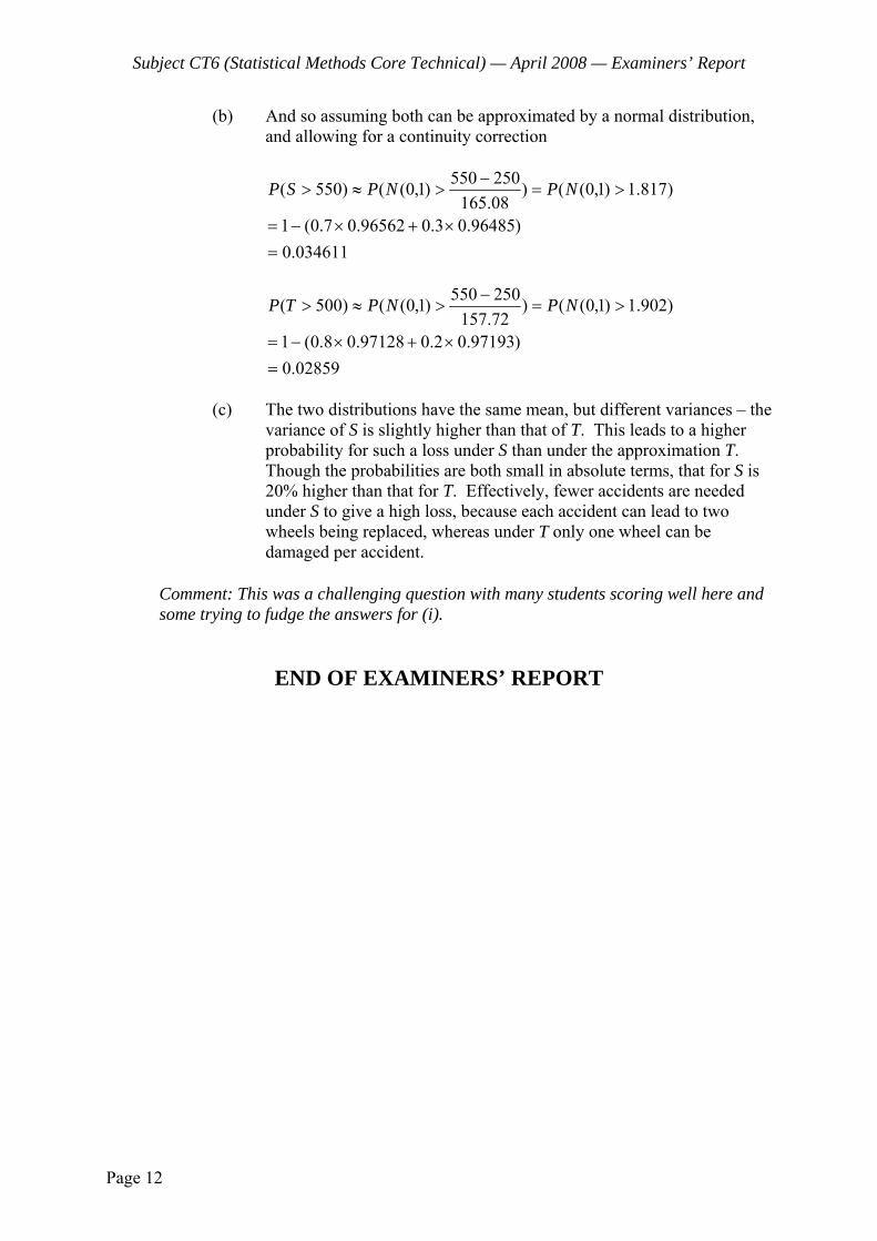
Subject CT6 (Statistical Methods Core Technical) — April 2008 — Examiners’ Report
Page 12
(b) And so assuming both can be approximated by a normal distribution, and allowing for a continuity correction
034611.0
)96485.03.096562.07.0(1
)817.1)1,0(()08.165250550)1,0(()550(
=×+×−=
>=−
>≈> NPNPSP
02859.0
)97193.02.097128.08.0(1
)902.1)1,0(()72.157250550)1,0(()500(
=×+×−=
>=−
>≈> NPNPTP
(c) The two distributions have the same mean, but different variances – the
variance of S is slightly higher than that of T. This leads to a higher probability for such a loss under S than under the approximation T. Though the probabilities are both small in absolute terms, that for S is 20% higher than that for T. Effectively, fewer accidents are needed under S to give a high loss, because each accident can lead to two wheels being replaced, whereas under T only one wheel can be damaged per accident.
Comment: This was a challenging question with many students scoring well here and some trying to fudge the answers for (i).
END OF EXAMINERS’ REPORT

Faculty of Actuaries Institute of Actuaries
EXAMINATION
16 September 2008 (am)
Subject CT6 — Statistical Methods Core Technical
Time allowed: Three hours
INSTRUCTIONS TO THE CANDIDATE
1. Enter all the candidate and examination details as requested on the front of your answer booklet.
2. You must not start writing your answers in the booklet until instructed to do so by the
supervisor. 3. Mark allocations are shown in brackets. 4. Attempt all 11 questions, beginning your answer to each question on a separate sheet. 5. Candidates should show calculations where this is appropriate.
Graph paper is not required for this paper.
AT THE END OF THE EXAMINATION
Hand in BOTH your answer booklet, with any additional sheets firmly attached, and this question paper.
In addition to this paper you should have available the 2002 edition of the Formulae and Tables and your own electronic calculator from the approved list.
© Faculty of Actuaries CT6 S2008 © Institute of Actuaries
CT6 S2008—2
1 Claim amounts on a portfolio of insurance policies have an unknown mean μ. Prior beliefs about μ are described by a distribution with mean μ0 and variance 2
0σ . Data are collected from n claims with mean claim amount x and variance s2. A credibility estimate of μ is to be made, of the form
0(1 )Zx Z+ − μ . Suggestions for the choice of Z are:
A 20
2 20
nn s
σ
σ +
B 20
20
nn n
σ
σ +
C 20
20n
σ
+σ
Explain whether each suggestion is an appropriate choice for Z. [4] 2 Write down the general statistical model for the run-off triangle claim data and
explain the terms used. [5] 3 An insurer is considering whether to outsource its advertising. If it decides not to
outsource, it expects to spend £1,400,000 next year on its advertising, and believes that this would result in a portfolio of 100,000 policies. It has received quotations from two different companies for outsourcing its advertising.
Company A would cost £2,100,000 per year, and believes that this would result in the
business expanding to 125,000 policies. Company B would cost £3,000,000 per year, and believes that this would expand the
business to 140,000 policies. At present, each policy returns a profit to the company of £30 per year; but this is not
guaranteed in the future. The company has assessed that it will stay at this level with probability 0.6, but could reduce to £20 per year with probability 0.25, or increase to £40 per year with probability 0.15.
(i) Explain which of the three options can be immediately discarded. [1] (ii) Determine the Bayes solution to the problem of maximising the profit to the
company over the coming year. [5] [Total 6]
CT6 S2008—3 PLEASE TURN OVER
4 An insurance company provides warranties for a certain electrical gadget. At the start of 2006 there were 4,500 gadgets under warranty, each of which has a probability q of suffering complete failure in 2006 (independently between gadgets). The prior distribution of q is beta with mean 0.015 and standard deviation 0.005. Given that 58 gadgets suffer a complete failure in 2006, determine the posterior distribution of q. [6]
5 The table below shows the cumulative values (in units of £1,000) of incurred claims
on a portfolio of an insurance company: Development year
Underwriting year 1 2 3 2005 3,541 7,111 9,501 2006 2,949 6,850 2007 3,894
The estimated loss ratio for 2006 and 2007 is 87% and the respective premium
income (also in units of £1,000) is: Premium income
2005 11,041 2006 11,314 2007 12,549
Given that the total of claims paid to date is £20,103,000, calculate the reserve for this
portfolio using the Bornhuetter-Ferguson method. [7] 6 Consider the ARCH(1) process
Xt = μ + et2
0 1 1( )tX −α +α −μ where et are independent normal random variables with variance 1 and mean 0. Show that, for s = 1, 2, … , t-1, Xt and Xt-s are: (i) uncorrelated. [5] (ii) not independent. [3] [Total 8]

CT6 S2008—4
7 (i) Let U1, U2, …, Un be independent random numbers generated from a U(0,1) distribution. Write down the Monte Carlo estimator, θ , for the integral
θ = 1
0( 1) .xe dx−∫ [1]
(ii) Determine the variance of the estimator θ in (i). [4] (iii) Calculate the smallest value of n for which the estimator θ has absolute error
less than 0.1 with probability 90%. [4] [Total 9] 8 An insurer has issued two five-year term assurance policies to two individuals
involved in a dangerous sport. Premiums are payable annually in advance, and claims are paid at the end of the year of death.
Individual Annual
Premium Sum Assured Annual
Prob (death) A 100 1,700 0.05 B 50 400 0.1
Assume that the probability of death is constant over each of the five years of the
policy. Suppose that the insurer has an initial surplus of U. (i) Define what is meant by ( )Uψ and ( , )U tψ . [2] (ii) Assuming U = 1,000 (a) Determine the distribution of S(1), the surplus at the end of the
first year, and hence calculate ( ,1)Uψ . (b) Determine the possible values of S(2) and hence calculate ( , 2)Uψ . [8] [Total 10]

CT6 S2008—5 PLEASE TURN OVER
9 A motor insurance company applies a NCD scale policy of discount levels
Level 0 0% Level 1 20% Level 2 50%
Following a claim-free year, the policyholder moves to the next higher level (or
remains at Level 2). If one or more claims are made, the policyholder moves to the next lower level (or remains at Level 0).
The probability of a policyholder not making a claim in a policy year is 1 - p. The annual premium at Level 0 is £600. (i) Derive, in terms of p, the expected proportions of policyholders at each
discount level assuming that the system is in equilibrium . [7] (ii) Calculate the average premium paid in the stable state for the particular values
p = 0.1 and p = 0.3 and comment on the results. [3] [Total 10]

CT6 S2008—6
10 From a sample of 50 consecutive observations from a stationary process, the table below gives values for the sample autocorrelation function (ACF) and the sample partial autocorrelation function (PACF):
Lag ACF PACF
1 0.854 0.854 2 0.820 0.371 3 0.762 0.085
The sample variance of the observations is 1.253. (i) Suggest an appropriate model, based on this information, giving your reasoning. [2] (ii) Consider the AR(1) model Yt = a1Yt-1 + et, where et is a white noise error term with mean zero and variance σ2. Calculate method of moments (Yule-Walker) estimates for the parameters of
a1 and σ2 on the basis of the observed sample. [4] (iii) Consider the AR(2) model Yt = a1Yt-1 + a2Yt-2 + et, where et is a white noise error term with mean zero and variance σ2. Calculate method of moments (Yule-Walker) estimates for the parameters of
a1 , a2 and σ2 on the basis of the observed sample. [7]
(iv) List two statistical tests that you should apply to the residuals after fitting a model to time series data. [2]
[Total 15]

CT6 S2008—7
11 Losses on a portfolio of insurance policies in 2006 are assumed to have an exponential distribution with parameter λ. In 2007 loss amounts have increased by a factor k (so that a loss incurred in 2007 is k times an equivalent loss incurred in 2006).
(i) Show that the distribution of loss amounts in 2007 is also exponential and
determine the parameter of the distribution. [3] Over the calendar years 2006 and 2007 the insurer had in place an individual excess-
of-loss reinsurance arrangement with a retention of M. Claims paid by the insurer were:
2006: 4 amounts of M and 10 claims under M for a total of 13,500. 2007: 6 amounts of M and 12 claims under M for a total of 17,000. (ii) Show that the maximum likelihood estimate of λ is:
22ˆ17,000 613,500 4 MM
k k
λ =+ + +
[7] (iii) The insurer is negotiating a new reinsurance arrangement for 2008. The
retention was set at 1600 when the current arrangement was put in place in 2006. Loss inflation between 2006 and 2007 was 10% (i.e. k = 1.1) and further loss inflation of 5% is expected between 2007 and 2008.
(a) Use this information to calculate λ . (b) The insurer wishes to set the retention M ′ for 2008 such that the
expected (net of re-insurance) payment per claim for 2008 is the same as the expected payment per claim for 2006. Calculate the value of M ′ , using your estimate of λ from (iii)(a). [10]
[Total 20]
END OF PAPER

Faculty of Actuaries Institute of Actuaries
Subject CT6 — Statistical Methods Core Technical
EXAMINERS’ REPORT
September 2008
Introduction The attached subject report has been written by the Principal Examiner with the aim of helping candidates. The questions and comments are based around Core Reading as the interpretation of the syllabus to which the examiners are working. They have however given credit for any alternative approach or interpretation which they consider to be reasonable. R D Muckart Chairman of the Board of Examiners November 2008
© Faculty of Actuaries © Institute of Actuaries
Subject CT6 (Statistical Methods Core Technical) — September 2008 — Examiners’ Report
Page 2
Comments on individual questions Q1 There was a wide variety in the standard of answers to this question – it was
generally well answered by the candidates who passed whilst weaker candidates struggled to relate the possible choices to the desirable characteristics of a credibility estimate.
Q2 This bookwork questions was generally well answered. Q3 Well answered. Q4 Many weaker candidates struggled to calculate α and β . Most were able to derive
the posterior distribution. Q5 Well answered. Q6 Candidates found this (and Q7) the hardest on the paper, with very few able to make
much headway. This was a little disappointing, since although the question was phrased around ARCH models it required only the standard definition on covariance and a little algebra.
Q7 Along with Q6, candidates found this the toughest question on the paper. Very few
were able to write down the required estimator and therefore made no progress at all. Many candidates failed to recognise that the estimator had to be a function of the uniform random variables rather than a fixed number.
Q8 This question was a good differentiator – the candidates who passed were able to take
a systematic approach to what was a fairly straightforward situation. Many weaker candidates failed to give an accurate definition of the probabilities in part (i) and a large number chose to make an approximation to the distribution in part(ii) when an exact calculation was simpler and quicker (and was what the question asked for).
The notation used in this question differed slightly from that used in the core reading,
which was unfortunate. Whilst this caused no problems for the majority of candidates, the examiners made allowance in those cases where the notation caused confusion.
Q9 This question was generally well answered. Q10 This question was well answered by the better candidates. Whilst most well prepared
candidates were able to derive the relevant Yule-Walker equations, only the better candidates were able to move from these to estimates for the parameters.
Q11 Another good differentiator. Most candidates were able to derive the maximum
likelihood estimate. Only the better candidates made much headway with part (iii).

Subject CT6 (Statistical Methods Core Technical) — September 2008 — Examiners’ Report
Page 3
1 A This is an appropriate choice – the larger the value of n, the closer Z is to 1 and the more weight is placed on the data. Furthermore, high values of the variance of the prior (indicating uncertainty in the prior) lead to higher values of Z and so more weight on the sample data. Finally, high variance in the sample reduces the value of Z and places more reliance on the prior.
B This is not appropriate – the value is a constant independent of the size of the
sample, whereas we would expect more weight on the sample the larger the sample.
C This is not appropriate – the greater the value of n, the lower the value of Z
and the less weight is put on the sample. This is the reverse of what we would expect.
2 Cij = Rj Si Xi+j + Eij where Cij is the incremental claims from origin year i to j years ahead. Rj is the development factor for year j independent of origin year i. Si is a parameter varying by origin year i, representing exposure (e.g. total
claims incurred). Xi+j is a parameter varying by calendar year, for example representing
inflation. Eij is the error term. 3 (i) Company B can be discounted immediately because it is dominated by both of
the other two options. (ii) Profit Table (in millions)
£20 £30 £40 E[Profit] Current 0.6 1.6 2.6 1.5 Company A 0.4 1.65 2.9 1.525
The insurer should choose Company A.

Subject CT6 (Statistical Methods Core Technical) — September 2008 — Examiners’ Report
Page 4
4 Suppose that q has a ( , )beta α β distribution as per the tables, and let X denote the number of failures in 2006 so that X has a B(4500,q) distribution. Then
1 1
1 1
( ) ( ) ( )
(1 ) (1 )
(1 )
x n x
x n x
f q X f q f X q
q q q q
q q
α− β− −
α+ − β+ − −
∝ ×
∝ − × −
∝ −
So the posterior distribution of q is beta with parameters xα + and n xβ+ − . In our case, the parameters of the prior distribution are given by
0.015α=
α +β and 2
2 0.005( ) ( 1)
αβ=
α +β α +β+.
0.015( )
0.985 0.0153
197
α = α +βα = β
α = β
And substituting into the second equation gives
22
2
22
3197 0.005
200 2001197 197
3 200 2000.005 1197 197 197
200591 1197
β=
⎛ ⎞ ⎛ ⎞β + β⎜ ⎟ ⎜ ⎟⎝ ⎠ ⎝ ⎠
⎛ ⎞ ⎛ ⎞= × × + β⎜ ⎟ ⎜ ⎟⎝ ⎠ ⎝ ⎠
= + β
197 11623590 581.15200 20
β = × = =
3 11623 8.85197 20
α = × =
So the revised parameters are given by: * 8.85 58 66.85α = + = * 581.15 4500 58 5023.15β = + − =

Subject CT6 (Statistical Methods Core Technical) — September 2008 — Examiners’ Report
Page 5
5 The main calculations are reported in the table:
Year
Initial ultimate. Loss r f 1 - 1/f
Emerging Liability
2006 9843.18 1.336099 1.336099 0.251552 2476.08 2007 10917.63 2.151156 2.874157=1.336099×2.151156 0.652072 7119.08
The second column (IUL) is obtained as 87% of Premium income values. The
third column reports the development factors 7111/9501 = 1.336099 and (7111 + 6850) / (3541 + 2949) = 2.151156. The emerging liability column is the product of IUL vales with those of 1 - 1/f. The total emerged liability is now 2476.08 + 7119.08 = 9595.16 and the total
reported liability is 9501 + 6850 + 3894 = 20245. Therefore the reserve value is 9595.16 + 20245 – 20103 = 9737.2.
6 (i) Since et are independent from Xt, Xt-1, … and E(et) = 0 we have that
20 1 1
20 1 1
20 1 1 1
20 1 1
( ) ( ( ) )
( ( ) )
( ) ( ( ) ) since and are independent
0 ( ( ) )
t t t
t t
t t t t
t
E X E e X
E e X
E e E X e X
E X
−
−
− −
−
= μ + α +α −μ
= μ + α +α −μ
= μ + α +α −μ
= μ + × α +α −μ
= μ
The direct approach to showing that tX and t sX − are uncorrelated is shown below. The crucial steps involve noting that te is independent of 1tX − as above, and that te is independent of
2 20 1 1 0 1 1( ) ( )t s t t se X X− − − −α +α −μ α +α −μ .
The algebra can be simplified by noting that adding a constant doesn’t affect covariance, so the μ ’s can be ignored.

Subject CT6 (Statistical Methods Core Technical) — September 2008 — Examiners’ Report
Page 6
( )2 2 20 1 1 0 1 1
2 2 20 1 1 0 1 1
2 2 20 1 1 0 1 1
2 20 1 1
( , ) ( ) ( ) ( )
( ( ) )( ( ) )
( ( ) ( )
( ) ( ) )
( ) ( ) ( ( ) )
t t s t t s t t s
t t t s t s
t t t s t s
t t s t s t
t t
Cov X X E X X E X E X
E e X e X
E e X e X
e e X X
E E e E X
− − −
− − − −
− − − −
− − − −
−
= −
= μ + α +α −μ μ + α +α −μ −μ
= μ +μ α +α −μ +μ α +α −μ
+ α +α −μ α +α −μ −μ
= μ +μ α +α −μ 20 1 1
2 2 20 1 1 0 1 1
2 2 20 1 1 0 1 1
2 2 20 1 1 0 1 1
( ) ( ( ) )
( ( ) ( ) )
0 ( ( ) ) 0 ( ( ) )
( ) ( ( ) ( ) )
t s t s
t t s t s t
t t s
t t s t s t
E e E X
E e e X X
E X E X
E e E e X X
− − −
− − − −
− − −
− − − −
+μ α +α −μ
+ α +α −μ α +α −μ −μ
= μ +μ× × α +α −μ +μ× × α +α −μ
+ α +α −μ α +α −μ −μ
2 2 2 20 1 1 0 1 1
0 0 0 ( ( ) ( ) )0
t s t s tE e X X− − − −= μ + + + × α +α −μ α +α −μ −μ
= (ii) The conditional variance of 1t tX X − is
1var( )t tX X − = var(et)(α0 + α1(Xt-1 -μ)2) = α0 + α1(Xt-1 - μ)2. So the values of Xt-1 are affecting the variance of Xt. If the same idea is
applied recursively, it can be seen that the variance of Xt will be affected by the value of Xt-s. So Xt and Xt-s are not independent.
7 (i) θ = 1
1 ( 1)tn
U
te
n =
−∑ = 1
1tn U
i
en=
⎛ ⎞−⎜ ⎟⎜ ⎟
⎝ ⎠∑
(ii) We need to find the variance of h(U) = eU -1 where U ~ U(0, 1)
Eh(U) = 1
0( 1)xe dx−∫ = e – 2
Eh(U)2 = 1 20
( 1)xe dx−∫
= 1 20
( 2 1)x xe e dx− +∫
= 2 1 2( 1) 12
e e−− − +
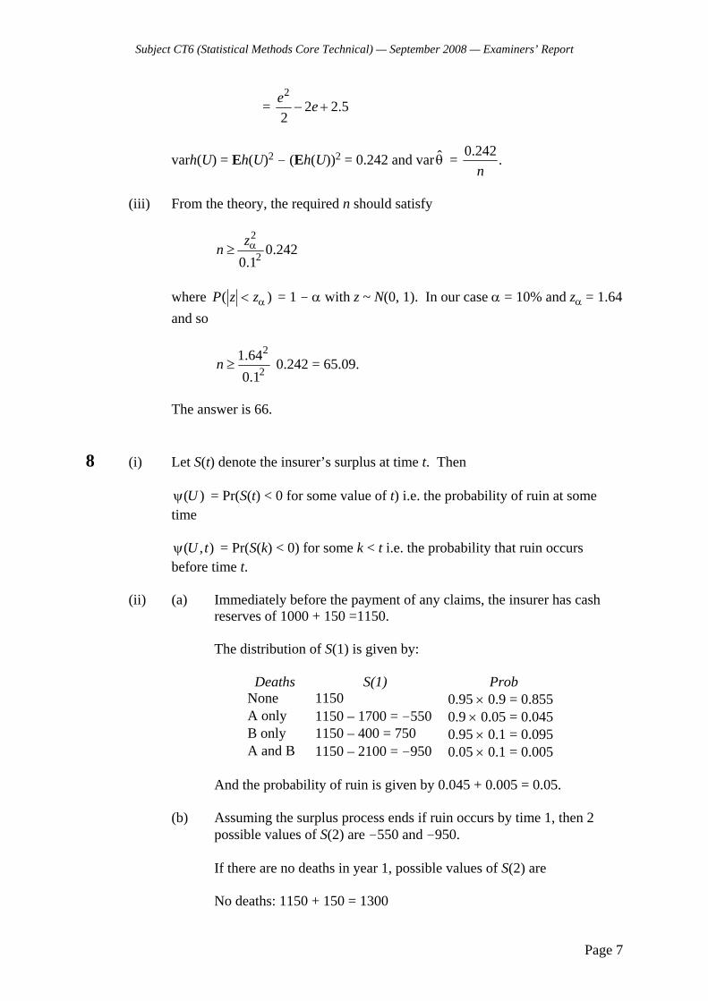
Subject CT6 (Statistical Methods Core Technical) — September 2008 — Examiners’ Report
Page 7
= 2
2 2.52e e− +
varh(U) = Eh(U)2 – (Eh(U))2 = 0.242 and var θ = 0.242 .n
(iii) From the theory, the required n should satisfy
2
2 0.2420.1zn α≥
where ( )P z zα< = 1 - α with z ~ N(0, 1). In our case α = 10% and zα = 1.64
and so
2
21.640.1
n ≥ 0.242 = 65.09.
The answer is 66. 8 (i) Let S(t) denote the insurer’s surplus at time t. Then ( )Uψ = Pr(S(t) < 0 for some value of t) i.e. the probability of ruin at some
time ( , )U tψ = Pr(S(k) < 0) for some k < t i.e. the probability that ruin occurs
before time t. (ii) (a) Immediately before the payment of any claims, the insurer has cash
reserves of 1000 + 150 =1150. The distribution of S(1) is given by:
Deaths S(1) Prob None 1150 0.95 × 0.9 = 0.855 A only 1150 – 1700 = -550 0.9 × 0.05 = 0.045 B only 1150 – 400 = 750 0.95 × 0.1 = 0.095 A and B 1150 – 2100 = -950 0.05 × 0.1 = 0.005
And the probability of ruin is given by 0.045 + 0.005 = 0.05. (b) Assuming the surplus process ends if ruin occurs by time 1, then 2
possible values of S(2) are -550 and -950. If there are no deaths in year 1, possible values of S(2) are No deaths: 1150 + 150 = 1300

Subject CT6 (Statistical Methods Core Technical) — September 2008 — Examiners’ Report
Page 8
A only: 1150 + 150 – 1700 = -400 B only: 1150 + 150 – 400 = 900 A and B: 1150 + 150 – 1700 – 400 = -800 If B dies in year 1, the possible values of S(2) are: A lives: 750 + 100 = 850 A dies: 750 + 100 – 1700 = -850 The probability of ruin within 2 years is given by: 0.05 + 0.855 × (0.05 × 0.9 + 0.05 × 0.1) + 0.095 × 0.05 = 0.0975 Alternatively, note that ruin occurs within 2 years if and only if A dies
during this time, the probability of which is 0.05 + 0.95 × 0.05 = 0.0975.
9 (i) The transition matrix is
1 0
0 10 1
p pp p
p p
−⎛ ⎞⎜ ⎟−⎜ ⎟⎜ ⎟−⎝ ⎠
The equilibrium probabilities ( 0π , 1π , 2π ) satisfy 0π = p 0π + p 1π 1π = 0π (1 - p) + p 2π 2π = 1π (1 - p) + (1 - p) 2π From equations 1 and 3 above we obtain 0π = p/(1 - p) 1π and 2π = (1 - p)/p 1π .
Since 0π + 1π + 2π =1 we get 1π = 2(1 )(1 )
p pp p
−+ −
together with 0π =2
2(1 )p
p p+ −
and 2π =2
2(1 )
(1 )p
p p−
+ −
(ii) The average premium is now
£600(2
2(1 )p
p p+ −+0.8 2
(1 )(1 )
p pp p
−+ −
+0.52
2(1 )
(1 )p
p p−
+ −) and for
p = 0.1 and p = 0.3 this quantity takes values £321.1 and £382 respectively.
Subject CT6 (Statistical Methods Core Technical) — September 2008 — Examiners’ Report
Page 9
The difference in average premiums is small given that the claim probability is three times higher, suggesting the NCD system does not discriminate well.
10 (i) ACF looks to decline exponentially suggesting an AR(p) process. While
PACF becomes almost zero at lag 3 so AR(2) is a likely process here. (ii) For p = 1 the equations are: γ1 = a1γ0 γ0 = a1γ1 + σ2 therefore 1a = 1ρ = 0.854 and 2 2
0 1 1 0 1ˆ ˆ ˆ ˆˆ ˆ (1 ) 0.33917.aσ = γ − γ = γ −ρ = (iii) For p = 2 the equations are: γ2 = a1γ1 + a2γ0 γ1 = a1γ0 + a2γ1 γ0 = a1γ1 + a2γ2 + σ2 Solving the first two equations with respect to ai after dividing both sizes by γ0
we have that
a2 = 2
2 1211
ρ −ρ
−ρ
a1 = ρ1(1 – a2) and with the right substitution for 1 2ˆ ˆ,ρ ρ we get 1 0.5679a = and 2ˆ 0.3350.a = Then the white noise variance can now be estimated as 2
0 1 1 2 2ˆ ˆ ˆˆ ˆ ˆ 0.3011.a aσ = γ − γ − γ = (iv) Any 2 tests can be given, including:
• the turning point’s test • the “portmanteau” Ljung-Box 2χ test • the inspection of the values of the SACF values based on their 95%
confidence intervals under the white noise null hypothesis

Subject CT6 (Statistical Methods Core Technical) — September 2008 — Examiners’ Report
Page 10
11 (i) Suppose X is exponentially distributed with parameter λ. Then we must show that Y = kX is also exponentially distributed.
Now ( ) ( )P Y y P kX y< = < ( / )P X y k= <
/
0
y kze dz−λ= λ∫
0
making the substitution zy x
k dxe x kk
λ−
= λ =∫
0
y xke dx
k
λ−λ
= ∫
Which is the distribution n function of an exponential distribution with
parameter / kλ . So Y is exponentially distributed with parameter / kλ . (ii) First note that the probability that a loss in 2006 is greater than M is given by
Me−λ and likewise the probability that a loss in 2007 is greater than M is given by /M ke−λ .
The likelihood of the data is given by:
/4 6 /( ) ( )i ix y kM M k
i jL C e e e e
k−λ −λ− λ − λ λ
= × × λ × ×∏ ∏
Where the ix represent the claims in 2006 and jy represent the claims in
2007. The log-likelihood is given by
log ' 4 10log 6 / 12log /
' 4 22log 13,500 6 / 17,000 /i jl L C M x M k k y
C M M k k
= = − λ + λ −λ − λ + λ −λ
= − λ + λ − λ − λ − λ∑ ∑
Differentiating gives
22' 4 13,500 6 / 17,000 /l M M k k= − + − − −λ
And equating this to zero gives ˆ4 22 / 13,500 6 / 17,000 / 0M M k k− + λ − − − =
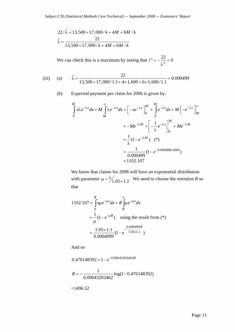
Subject CT6 (Statistical Methods Core Technical) — September 2008 — Examiners’ Report
Page 11
ˆ22 / 13,500 17,000 / 4 6 /k M M kλ = + + +
22ˆ13,500 17,000 / 4 6 /k M M k
λ =+ + +
We can check this is a maximum by noting that 222'' 0l = − <λ
(iii) (a) 22ˆ 0.00049913,500 17,000 /1.1 4 1,600 6 1,600 /1.1
λ = =+ + × + ×
(b) Expected payment per claim for 2006 is given by:
0
0 0
M MMx x x x xM
M
x e dx M e dx xe e dx M e∞ ∞−λ −λ −λ −λ −λ⎡ ⎤ ⎡ ⎤λ + λ = − + + −⎣ ⎦ ⎣ ⎦∫ ∫ ∫
0
1 MM x MMe e Me−λ −λ −λ⎡ ⎤= − + − +⎢ ⎥λ⎣ ⎦
1 (1 ) (*)Me−λ= −λ
0.000499 16001 (1 )0.000499
e− ×= −
1102.107= We know that claims for 2008 will have an exponential distribution
with parameter 1.05 1.1λμ = × . We need to choose the retention R so
that
0
1102.107R
x x
R
x e dx R e dx∞
−μ −μ= μ + μ∫ ∫
1 (1 ) using the result from (*)Re−μ= −μ
0.000499
1.05 1.11.05 1.1 (1 )0.0004999
R
e−
××= −
And so 0.000432034630.476148392 1 Re−= −
1 log(1 0.476148392)0.00043203462
R = − −
=1496.52

Subject CT6 (Statistical Methods Core Technical) — September 2008 — Examiners’ Report
Page 12
END OF EXAMINERS’ REPORT

Faculty of Actuaries Institute of Actuaries
EXAMINATION
28 April 2009 (am)
Subject CT6 — Statistical Methods Core Technical
Time allowed: Three hours
INSTRUCTIONS TO THE CANDIDATE
1. Enter all the candidate and examination details as requested on the front of your answer booklet.
2. You must not start writing your answers in the booklet until instructed to do so by the
supervisor. 3. Mark allocations are shown in brackets. 4. Attempt all 11 questions, beginning your answer to each question on a separate sheet. 5. Candidates should show calculations where this is appropriate.
Graph paper is not required for this paper.
AT THE END OF THE EXAMINATION
Hand in BOTH your answer booklet, with any additional sheets firmly attached, and this question paper.
In addition to this paper you should have available the 2002 edition of the Formulae and Tables and your own electronic calculator from the approved list.
© Faculty of Actuaries CT6 A2009 © Institute of Actuaries
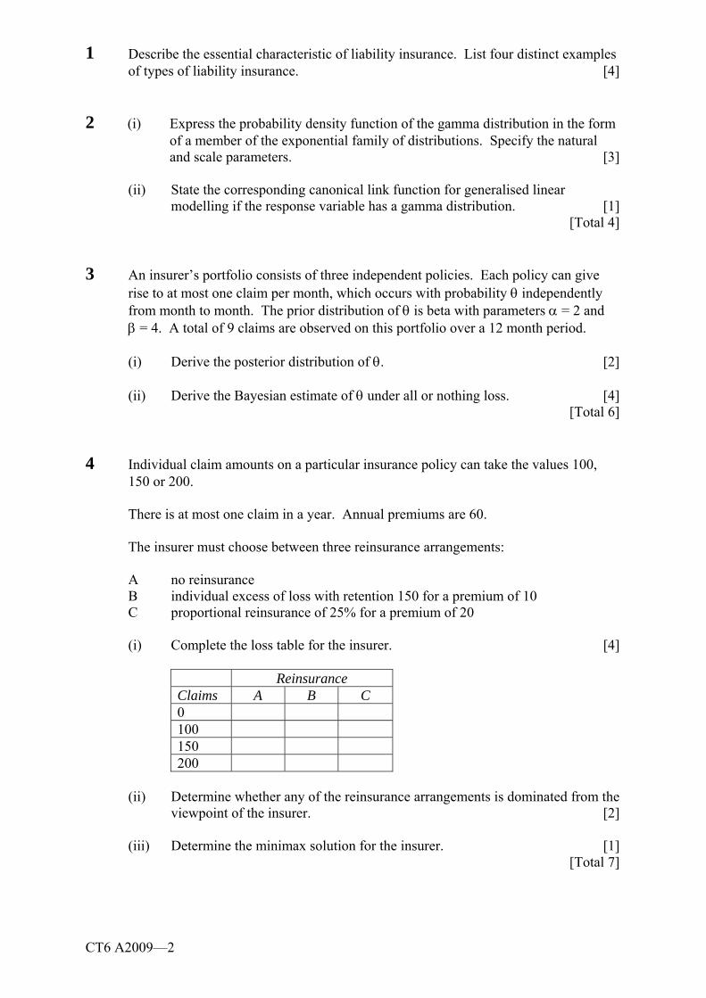
CT6 A2009—2
1 Describe the essential characteristic of liability insurance. List four distinct examples of types of liability insurance. [4]
2 (i) Express the probability density function of the gamma distribution in the form
of a member of the exponential family of distributions. Specify the natural and scale parameters. [3]
(ii) State the corresponding canonical link function for generalised linear
modelling if the response variable has a gamma distribution. [1] [Total 4] 3 An insurer’s portfolio consists of three independent policies. Each policy can give
rise to at most one claim per month, which occurs with probability θ independently from month to month. The prior distribution of θ is beta with parameters α = 2 and β = 4. A total of 9 claims are observed on this portfolio over a 12 month period.
(i) Derive the posterior distribution of θ. [2] (ii) Derive the Bayesian estimate of θ under all or nothing loss. [4] [Total 6] 4 Individual claim amounts on a particular insurance policy can take the values 100,
150 or 200. There is at most one claim in a year. Annual premiums are 60. The insurer must choose between three reinsurance arrangements: A no reinsurance B individual excess of loss with retention 150 for a premium of 10 C proportional reinsurance of 25% for a premium of 20 (i) Complete the loss table for the insurer. [4]
Reinsurance Claims A B C 0 100 150 200
(ii) Determine whether any of the reinsurance arrangements is dominated from the
viewpoint of the insurer. [2] (iii) Determine the minimax solution for the insurer. [1] [Total 7]
CT6 A2009—3 PLEASE TURN OVER
5 An insurance portfolio contains policies for three categories of policyholder: A, B and C. The number of claims in a year, N, on an individual policy follows a Poisson distribution with mean λ. Individual claim sizes are assumed to be exponentially distributed with mean 4 and are independent from claim to claim. The distribution of λ, depending on the category of the policyholder, is
Category Value of λ Proportion of policyholders
A 2 20% B 3 60% C 4 20%
Denote by S the total amount claimed by a policyholder in one year. (i) Prove that ( ) [ ( )]E S E E S= λ . [2] (ii) Show that ( ) 4E S λ = λ and Var( ) 32S λ = λ . [2] (iii) Calculate E(S). [2] (iv) Calculate Var(S). [2] [Total 8] 6 The following information is available for a motor insurance portfolio: The number of claims settled: Development Year
Accident year 0 1 2 2006 442 151 50 2007 623 111 2008 681
The cost of settled claims during each year (in 000’s): Development Year
Accident year 0 1 2 2006 6321 1901 701 2007 7012 2237 2008 7278
Claims are fully run off after year 2. Calculate the outstanding claims reserve using
the average cost per claim method with grossing up factors. Inflation can be ignored. [10]

CT6 A2009—4
7 It is necessary to simulate samples from a distribution with density function ( ) 6 (1 ) 0 1f x x x x= − < < .
(i) Use the acceptance-rejection technique to construct a complete algorithm for
generating samples from f by first generating samples from the distribution with density ( ) 2(1 )h x x= − . [5]
(ii) Calculate how many samples from h would on average be needed to generate
one realisation from f. [1] (iii) Explain whether the acceptance-rejection method in (i) would be more
efficient if the uniform distribution were to be used instead. [4] [Total 10] 8 An insurer has an initial surplus of U. Claims up to time t are denoted by S(t).
Annual premium income is received continuously at a rate of c per unit time. (i) Explain what is meant by the insurer’s surplus process U(t). [2]
(ii) Define carefully each of the following probabilities: (a) ( , )U tψ (b) ( , )h U tψ [2] (iii) Explain, for each of the following pairs of expressions, whether one of each
pair is certainly greater than the other, or whether it is not possible to reach a conclusion.
(a) (10,2)ψ and (20,1)ψ (b) (10,2)ψ and (5,1)ψ (c) 0.5(10,2)ψ and 0.25(10,2)ψ
[6] [Total 10]
CT6 A2009—5 PLEASE TURN OVER
9 Individual claims under a certain type of insurance policy are for either 1 (with probability α) or 2 (with probability 1 − α).
The insurer is considering entering into an excess of loss reinsurance arrangement
with retention 1 + k (where k < 1). Let iX denote the amount paid by the insurer (net of reinsurance) on the ith claim.
(i) Calculate and simplify expressions for the mean and variance of iX . [5] Now assume that 0.2α = . The number of claims in a year follows a Poisson
distribution with mean 500. The insurer wishes to set the retention so that the probability that aggregate claims in a year will exceed 700 is less than 1%.
(ii) Show that setting k = 0.334 gives the desired result for the insurer. [5] [Total 10]
10 Let Yt be a stationary time series with autocovariance function ( )Y sγ . (i) Show that the new series Xt = a + bt +Yt where a and b are fixed non-zero
constants, is not stationary. [2] (ii) Express the autocovariance function of ΔXt = Xt − Xt−1 in terms of ( )Y sγ and
show that this new series is stationary. [7] (iii) Show that if Yt is a moving average process of order 1, then the series ΔXt is
not invertible and has variance larger than that of Yt. [6] [Total 15]

CT6 A2009—6
11 A motor insurance company operates a No Claims Discount scheme with discount levels 0%, 25% and 50% of the annual premium of 1,000. The probability of having an accident during any year is 0.1 (ignore the possibility of more than one accident in a year). The policyholder moves one level up in the discount scheme (or stays at the 50% level) in the event of a claim free year and moves one level down (or stays at the 0% level) if the claim does not involve a criminal offence. If the claim involves a criminal offence then the policyholder automatically moves to the 0% discount level. One in ten accidents involves a criminal offence. The policyholder makes a claim only if the cost of repairs is higher than the aggregate additional premiums payable in the next two claim-free years.
(i) Calculate, for each level of discount, the cost of a repair below which the
policyholder will not claim, distinguishing between claims that involve a criminal offence and claims that do not. [4]
(ii) Calculate the probability of a claim for each level of discount given that an
accident has occurred, given that the repair cost following an accident has an exponential distribution with mean 400. [5]
(iii) Calculate the stationary distribution of the proportion of policyholders at each
discount level. [7] [Total 16]
END OF PAPER

Faculty of Actuaries Institute of Actuaries
Subject CT6 — Statistical Methods Core Technical
EXAMINERS’ REPORT
April 2009
Introduction The attached subject report has been written by the Principal Examiner with the aim of helping candidates. The questions and comments are based around Core Reading as the interpretation of the syllabus to which the examiners are working. They have however given credit for any alternative approach or interpretation which they consider to be reasonable. R D Muckart Chairman of the Board of Examiners June 2009
© Faculty of Actuaries © Institute of Actuaries

Subject CT6 — Statistical Methods Core Technical — April 2009 — Examiners’ Report
Page 2
Comments Comments on solutions presented to individual questions for this April 2009 paper are given below. Q1 This was generally well answered with various examples for liability insurance
mentioned. Q2 This is a standard theoretical question. Many candidates scored full marks here. Q3 Many candidates misspecified the parameters of the Beta distribution in (i) Q4 Some candidates ignored the premium of 60 so all their figures were out by this
amount. This however did not affect the answers in (ii) and (iii). Q5 Part (i) was generally not well answered despite the fact that it is a standard result
about conditional expectations. Alternative correct solutions were also presented. The following parts of the question were straightforward.
Q6 This question was well answered with many candidates scoring full marks. The final
figures could differ from those shown in the model solution due to differences in rounding in the intermediate steps. Full credit was given for these provided a consistent approach was taken to rounding.
Q7 Many candidates were able to give a correct general idea, but very few were able to
specify a complete algorithm so that not many scored full marks. Q8 This was a straightforward question where many candidates scored well. Q9 Many marks were dropped in the last stages of the solution. Q10 This was one of the least well answered questions and many marks were dropped
particularly in parts (ii) and (iii). Q11 Many candidates scored well here despite the lengthy calculations required. Some
however dropped marks at the calculation of P(claim/accident) at the 50% discount level because they did not distinguish between the cases where the accident was due to a criminal offences and those where it was not.

Subject CT6 — Statistical Methods Core Technical — April 2009 — Examiners’ Report
Page 3
1 The essential characteristic of liability insurance is to provide indemnity where the insured, owing to some form of negligence, is legally liable to pay compensation to a third party.
Examples
• Employer’s liability • Motor 3rd party liability • Public liability • Product liability • Professional indemnity
2 (i) We need to express the distribution function of the Gamma distribution in the
form:
( ( ))( ; , ) exp ( , )( )Y
y bf y c ya
⎡ ⎤θ − θθ ϕ = + ϕ⎢ ⎥ϕ⎣ ⎦
Suppose Y has a Gamma distribution with parameters α and λ . Then
1( )
( )y
Yf y y eα
α− −λλ=Γ α
And substituting αλ =
μ we can write the density as
1( ; , )( )
y
Yf y y eαα −
α− μαα
θ ϕ =μ Γ α
( ; , ) exp log ( 1) log log log ( )Yyf y y
⎡ ⎤⎛ ⎞θ ϕ = − − μ α + α − +α α − Γ α⎢ ⎥⎜ ⎟μ⎝ ⎠⎣ ⎦
Which is in the right form with 1θ = −
μ; ϕ = α ; 1( )a ϕ =
ϕ; ( ) log( )b θ = − −θ
and ( , ) ( 1) log log log ( )c y yϕ = ϕ− + ϕ ϕ− Γ ϕ .
Thus the natural parameter is 1μ
, ignoring the minus sign, and the scale
parameter is .α
(ii) The corresponding link function is 1μ
.

Subject CT6 — Statistical Methods Core Technical — April 2009 — Examiners’ Report
Page 4
3 (i) ( )f xθ ( ) ( )f x f∝ θ θ
9 27 1 1(1 ) (1 )α− β−∝ θ −θ θ −θ
9 27 1 3(1 ) (1 )∝ θ −θ θ −θ
10 30(1 )∝ θ −θ
Which is the pdf of a Beta(11,31) distribution. (ii) Under all or nothing loss, the Bayes estimate is the value that maximises the
pdf of the posterior.
( )f θ 10 30(1 )C= ×θ −θ
( )f ′ θ ( )9 30 10 2910 (1 ) 30(1 ) 1C= θ −θ + θ × −θ ×−
( )9 29(1 ) 10(1 ) 30C= θ − θ − θ − θ And ( ) 0f ′ θ = when 10(1 ) 30 0− θ − θ = 40 10θ = 1/ 4θ = We can check this is a maximum by observing that f(0.25) > 0 whilst f(0) = f(1) = 0. Since the maximum on [0,1] must occur either at the end-
points of the interval, or at turning point we can see that we do have a maximum.
4 (i) The loss table is as follows:
Claims Impact of reinsurance Insurer’s Loss A B C A B C 0 0 −10 −20 −60 −50 −40 100 0 −10 5 40 50 35 150 0 −10 17.5 90 100 72.5 200 0 40 30 140 100 110
(ii) If there are no claims, A gives the best result. If claims are 100 C gives the best result. If claims are 200 then B gives the best result. So each strategy can be best under certain circumstances, and so no approach
is dominated.

Subject CT6 — Statistical Methods Core Technical — April 2009 — Examiners’ Report
Page 5
(iii) The maximum losses are: A 140 B 100 C 110 The lowest is for B, so approach B is the minimax solution. 5 (i) Let ( )f s denote the marginal probability density for S and let ( )f s λ denote
the conditional probability density for S λ . Then
[ ( )]E E S λ 3
1 0
( ) ( )ii
p sf s ds∞
=
= λ λ∑ ∫
3
10
( ) ( )ii
s p f s ds∞
=
= λ λ∑∫
But 3
1( ) ( ) ( )i
ip f s f s
=
λ λ =∑ by definition, so
( )0
( ) ( )E E S sf s ds E S∞
⎡ ⎤λ = =⎣ ⎦ ∫
(ii) Using the results for compound distributions, we have: ( ) ( ) ( ) ( ) ( ) 4E S E N E X E N E Xλ = λ λ = λ = λ 2( ) ( ) ( ) ( ) ( )Var S E N Var X Var N E Xλ = λ + λ
216 4= λ× + λ× 32= λ (iii) ( ) [ ( )] (4 ) 4 ( ) 12E S E E S E E= λ = λ = λ =

Subject CT6 — Statistical Methods Core Technical — April 2009 — Examiners’ Report
Page 6
(iv) First note that ( ) 3E λ = and 2 2 2( ) 0.2 2 0.6 3 0.2 4 9 0.4Var λ = × + × + × − = ( ) [ ( )] [ ( )]Var S Var E S E Var S= λ + λ (4 ) (32 )Var E= λ + λ 16 ( ) 32 ( )Var E= × λ + λ 16 0.4 32 3= × + × 102.4= 6 The accumulated claims are:
Development Year Accident year 0 1 2 Ult
2006 442 593 643 643 2007 623 734 796 2008 681 927
The accumulated claim costs are:
Development Year Accident year 0 1 2
2006 6321 8222 8923 2007 7012 9249 2008 7278
The average costs per claim are:
Development Year Accident year 0 1 2 Ult
2006 14.301 13.865 13.877 13.877 2007 11.255 12.601 12.612 2008 10.687 11.115
The grossing-up factors for the claim numbers:
Accident year 0 1 2 2006 0.687 0.922 1 2007 0.783 0.922 2008 0.735

Subject CT6 — Statistical Methods Core Technical — April 2009 — Examiners’ Report
Page 7
The grossing-up factors for the average cost per settled claim:
Accident year 0 1 2 2006 1.031 0.999 1 2007 0.892 0.999 2008 0.961
Projected loss: 643 × 13.877 + 796 × 12.612 + 927 × 11.115 = 29265.67 Claims paid to date: 8923 + 9249 + 7278 = 25450 Outstanding Claims are therefore: 3815.7
The calculations are based on rounding the intermediate calculations to the accuracy shown. Different rounding will give slightly different answers, and is acceptable. Carrying all the calculations through in full accuracy gives a solution of 3808.0.
7 (i) We must find C where
( ) 6 (1 )max max 3 3( ) 2(1 )
f x x xC Max xh x x
−= = = =
−
We need to be able to generate a random variable from the distribution with
density h(x). We can do this as follows. First note that the cdf of h(x) is
2 20
0 0
( ) ( ) 2(1 ) 2 2x x x
H x g t dt t dt t t x x⎡ ⎤= = − = − = −⎣ ⎦∫ ∫
Given a random sample z from U(0,1) we can use the inverse transform
method to sample from h by setting:
2
2
2
2 0
2 4 4 1 12
x x z
x x z
zx z
− =
− + =
± −= = ± −
And we can see that the solution we want is 1 1x z= − − The algorithm to generate a sample y from f is then:
• Sample z from U(0,1) • Generate x from h(x) via 1 1x z= − − • Generate u from U(0,1)
• If ( ) 6 (1 )3 ( ) 6(1 )f x x xu xh x x
−< = =
− then generate y = x otherwise begin again.
Subject CT6 — Statistical Methods Core Technical — April 2009 — Examiners’ Report
Page 8
(ii) On average, we expect to use C = 3 realisations from h to generate one sample from f.
(iii) In this case, we must find the maximum value of f(x). ( ) 6 12f x x′ = − And f ′ (x) = 0 when x = 0.5 Since f(0) = f(1) = 0 and f(0.5) = 6/4 = 1.5 we can see that this is the
maximum. Since C is lower for g(x) = 1, using the constant function would be more
efficient. 8 (i) U(t) represents the insurers surplus at time t. It represents the initial surplus
plus cumulative premiums received less claims incurred: ( ) ( )U t U ct S t= + − Where U is the initial surplus and c is the annual premium income (assumed
payable continuously). (ii) (a) ( , ) ( ( ) 0 for some 0 given that (0) )U t P U s s t U Uψ = < ≤ ≤ = (b) ( , ) ( ( ) 0 for some , , 2 , , , h U t P U s s s h h t h tψ = < = −… given that (0) )U U= (iii) (a) We can say that (10, 2) (10,1) (20,1)ψ > ψ > ψ The first inequality holds because the longer the period considered
when checking, the more likely that ruin will occur. The second inequality holds because a larger initial surplus reduces the probability of ruin (higher claims are required to cause ruin).
(b) We can reach no definite conclusion here. The first term has a longer
term suggesting a higher probability, but a higher initial surplus suggesting a lower probability. We can’t say anything about the size of the two effects, so we can’t reach a definite conclusion.
(c) We can say that 0.5 0.25(10,2) (10,2)ψ ≤ ψ . This is because the second term checks for ruin at the same times as the first
term, as well as at some additional times. So the probability of ruin when checking over the larger set of times must be higher.
Subject CT6 — Statistical Methods Core Technical — April 2009 — Examiners’ Report
Page 9
9 (i) ( )iE X = (1 )(1 )kα + + −α = 1 (1 )k+ −α ( )iVar X = 2 2( ) ( )i iE X E X−
= 2 2(1 ) (1 ) (1 (1 ))k kα+ + −α − + −α
= 2 2 2(1 ) 2 (1 ) (1 ) 1 2 (1 ) (1 )k k k kα+ −α + −α + −α − − −α − −α
= 2(1 )(1 (1 ))k −α − −α
2 (1 )k= α −α (ii) Let Y denote the aggregate claims in a year. Then Y has a compound Poisson
distribution, and using the standard results from the tables: ( ) 500 ( ) 500 500 (1 ) 500 400iE Y E X k k= × = + −α = + =633.60 And ( )Var Y = 2500 ( )iE X×
= ( )2500 (1 ) (1 )kα+ + −α
= ( )2500 (1 ) 2 (1 ) (1 )k kα+ −α + −α + −α
= 2500 (1000 500 )(1 )k k+ + −α
= 2500 800 400k k+ + = 811.82 Using a normal approximation, we find
700 633.6( 700) ( )811.82
P Y P Z −> = >
( 2.33)P Z= > = 0.01 10 (i) Since tY is stationary, we know there is a constant Yμ such that ( )t YE Y = μ
for all values of t. But then ( ) ( )t t YE X E a bt Y a bt= + + = + +μ which depends on t since b is
non-zero. Hence tX is not stationary.

Subject CT6 — Statistical Methods Core Technical — April 2009 — Examiners’ Report
Page 10
(ii) First note that 1( ) ( )t t tE X E X X −Δ = − 1( ) ( )t tE X E X −= − 1( ) ( ( 1) )t tE a bt Y E a b t Y −= + + − + − + ( 1)Y Ya bt a b t= + +μ − − − −μ b= i.e. the mean is a constant independent of t. Secondly, ( , )t t sCov X X −Δ Δ = 1 1( , )t t t s t sCov X X X X− − − −− − 1 1( , )t t t s t sCov b Y Y b Y Y− − − −= + − + − 1 1( , )t t t s t sCov Y Y Y Y− − − −= − − 1 1 1 1( , ) ( , ) ( , ) ( , )t t s t t s t t s t t sCov Y Y Cov Y Y Cov Y Y Cov Y Y− − − − − − − −= − − + ( ) ( 1) ( 1) ( )Y Y Y Ys s s s= γ − γ − − γ + + γ 2 ( ) ( 1) ( 1)Y Y Ys s s= γ − γ − − γ + Since the autocovariance depends only on the lag s, and the mean is constant,
the new series is stationary. (iii) Suppose that 1t t tY e e −= +β where te is a white noise process with variance
2σ . Then 1 1 2( 1)t t t t tX a bt e e a b t e e− − −Δ = + + +β − − − − −β 1 2( 1)t t tb e e e− −= + + β− −β
2(1 ( 1) ) tb B B e= + + β− −β (1 )(1 ) tb B B e= + − +β So the lag polynomial has a unit root, and hence the time series is not
invertible. Now 1( ) ( )t t tVar Y Var e e −= +β
21( ) ( )t tVar e Var e −= +β
2 2(1 )= +β σ So 2 2(0) (1 )Yγ = +β σ

Subject CT6 — Statistical Methods Core Technical — April 2009 — Examiners’ Report
Page 11
Also 21 1 2(1) ( 1) ( , )Y Y t t t tCov e e e e− − −γ = γ − = +β +β = βσ
So using the result from part (ii) ( ) 2 (0) (1) ( 1)t Y Y YVar XΔ = γ − γ − γ −
2 2 22(1 ) 2= +β σ − βσ
2 22(1 )= −β+β σ And finally 2 2 2 2( ) ( ) (2 2 2 ) (1 )t tVar X Var YΔ − = − β+ β σ − +β σ
2 2(1 2 )= − β+β σ
2 2(1 ) 0= −β σ > 11 (i) Premiums at the three levels are £1,000, £750 and £500. 0% level Claims involving criminal offences make no difference here. Claim: 1000 + 750 = 1750 No Claim: 750 + 500 = 1250 No claim if the accident cost is less than 500. 25% level Claims involving criminal offences make no difference here. Claim: 1000 + 750 = 1750 No Claim: 500 + 500 = 1000 No claim if the accident cost is less than 750. 50% level Criminal offence claims make a difference here so we distinguish two
scenarios: No criminal offence Claim: 750 + 500 = 1250 Not claim: 500 + 500 = 1000 No claim if the accident cost is less than 250.

Subject CT6 — Statistical Methods Core Technical — April 2009 — Examiners’ Report
Page 12
Criminal offence Claim: 1000 + 750 = 1750 Not claim: 500 + 500 = 1000 No claim if the accident cost is less than 750.
(ii) Let X be the repair cost for each accident then 1~400
X Exp ⎛ ⎞⎜ ⎟⎝ ⎠
i.e. P(X > x) = 400x
e−
For 0% level: P(claim|accident) = P(X > 500) = 54e
−= 0.2865
For 25% level: P(claim|accident) = P(X > 750) = 7540e
− = 0.1534
For 50% level: P(claim|accident) = P(claim|criminal offence) + P(claim| no criminal offence) = P(X > 750) × 0.1 + P(X > 250) × 0.9
= 75400.1e
−+
25400.9e
−= 0.4971
(iii) Note that P(Accident) = 0.1 and P(criminal offence| accident) = 0.1. Hence at 0% level: P11 = P(current level) = P(make a claim) = P(claim|accident) P(accident) = 0.02865 P12 = P(move to 25% level) = P(not claim) = 1 − 0.02865 = 0.97135 P13 = P(move to 50% level) = 0 At 25% level: P21 = P(move down to 0% level) = P(make a claim) = P(claim|accident) P(accident) = 0.015335 P22 = 0 since it can never remain at this level for more than a year at a time P23 = 1 − P21 = 1 − 0.015335 = 0.984665
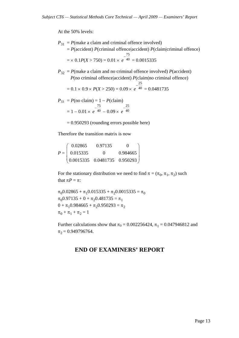
Subject CT6 — Statistical Methods Core Technical — April 2009 — Examiners’ Report
Page 13
At the 50% levels: P31 = P(make a claim and criminal offence involved) = P(accident) P(criminal offence|accident) P(claim|criminal offence)
= × 0.1P(X > 750) = 0.01 × 7540e
− = 0.0015335
P32 = P(make a claim and no criminal offence involved) P(accident) P(no criminal offence|accident) P(claim|no criminal offence)
= 0.1 × 0.9 × P(X > 250) = 0.09 × 2540e
− = 0.0481735
P33 = P(no claim) = 1 − P(claim)
= 1 − 0.01 × 7540e
− − 0.09 ×
2540e
−
= 0.950293 (rounding errors possible here) Therefore the transition matrix is now
P = 0.02865 0.97135 00.015335 0 0.9846650.0015335 0.0481735 0.950293
⎛ ⎞⎜ ⎟⎜ ⎟⎜ ⎟⎝ ⎠
For the stationary distribution we need to find π = (π0, π1, π2) such that πP = π: π00.02865 + π10.015335 + π20.0015335 = π0 π00.97135 + 0 + π20.481735 = π1 0 + π10.984665 + π20.950293 = π2 π0 + π1 + π2 = 1 Further calculations show that π0 = 0.002256424, π1 = 0.047946812 and π2 = 0.949796764.
END OF EXAMINERS’ REPORT

Faculty of Actuaries Institute of Actuaries
EXAMINATION
7 October 2009 (am)
Subject CT6 — Statistical Methods Core Technical
Time allowed: Three hours
INSTRUCTIONS TO THE CANDIDATE
1. Enter all the candidate and examination details as requested on the front of your answer booklet.
2. You must not start writing your answers in the booklet until instructed to do so by the
supervisor. 3. Mark allocations are shown in brackets. 4. Attempt all 10 questions, beginning your answer to each question on a separate sheet. 5. Candidates should show calculations where this is appropriate.
Graph paper is not required for this paper.
AT THE END OF THE EXAMINATION
Hand in BOTH your answer booklet, with any additional sheets firmly attached, and this question paper.
In addition to this paper you should have available the 2002 edition of the Formulae and Tables and your own electronic calculator from the approved list.
© Faculty of Actuaries CT6 S2009 © Institute of Actuaries

CT6 S2009—2
1 Consider the stationary autoregressive process of order 1 given by
12t t tY Y Z−= α + , 0.5α < where Zt denotes white noise with mean zero and variance σ2.
Express Yt in the form 0
t j t jj
Y a Z∞
−=
= ∑ and hence or otherwise find an expression for
the variance of Yt in terms of α and σ. [4] 2 An insurance company has a portfolio of two-year policies. Aggregate annual claims
from the portfolio follow an exponential distribution with mean 10 (independently from year to year). Annual premiums of 15 are payable at the start of each year. The insurer checks for ruin only at the end of each year. The insurer starts with no capital. Calculate the probability that the insurer is not ruined by the end of the second year. [5]
3 The loss function under a decision problem is given by:
1θ 2θ 3θ d1 10 15 5 d2 8 20 15 d3 12 15 10 d4 5 23 8
where d1, d2, d3 and d4 are the possible decisions and 1θ , 2θ and 3θ are the possible states of nature.
(i) State which decision can be discounted immediately. [1] (ii) Determine the minimax solution to the problem. [2] (iii) Determine the Bayes criterion solution to the problem given that 1( ) 0.4P θ = ,
2( ) 0.25P θ = and 3( ) 0.35P θ = . [2] [Total 5]

CT6 S2009—3 PLEASE TURN OVER
4 A portfolio consists of k independent travel insurance policies. Each policy covers the policyholder’s trips over one year. For policy i, the number of claims in the jth month of the covered year, ijY , is assumed to have a distribution given by
( ) (1 ) for 0,1,2,y
ij ij ijP Y y y= = θ −θ = …
where ijθ are unknown constants between 0 and 1. (i) Write down the likelihood function and obtain the maximum likelihood
estimate for the parameters ijθ . [3] (ii) Show that ( )ijP Y y= can be written in exponential family form and suggest its
natural parameter. [2] (iii) Suppose that ijθ depends on the temperature jx recorded in the jth month.
Explain why it is not appropriate to set ij jxθ = α +β . Suggest another
relationship between ijθ and jxα +β that might be used. [3] [Total 8] 5 The following claim amounts are believed to come from a lognormal distribution with
unknown parameters μ and σ2:
50, 87, 103, 119, 126, 154, 183, 203 Estimate the parameters μ and σ2 using: (i) the method of moments; [5] (ii) the method of percentiles, using the upper and lower quartiles. [5] [Total 10]
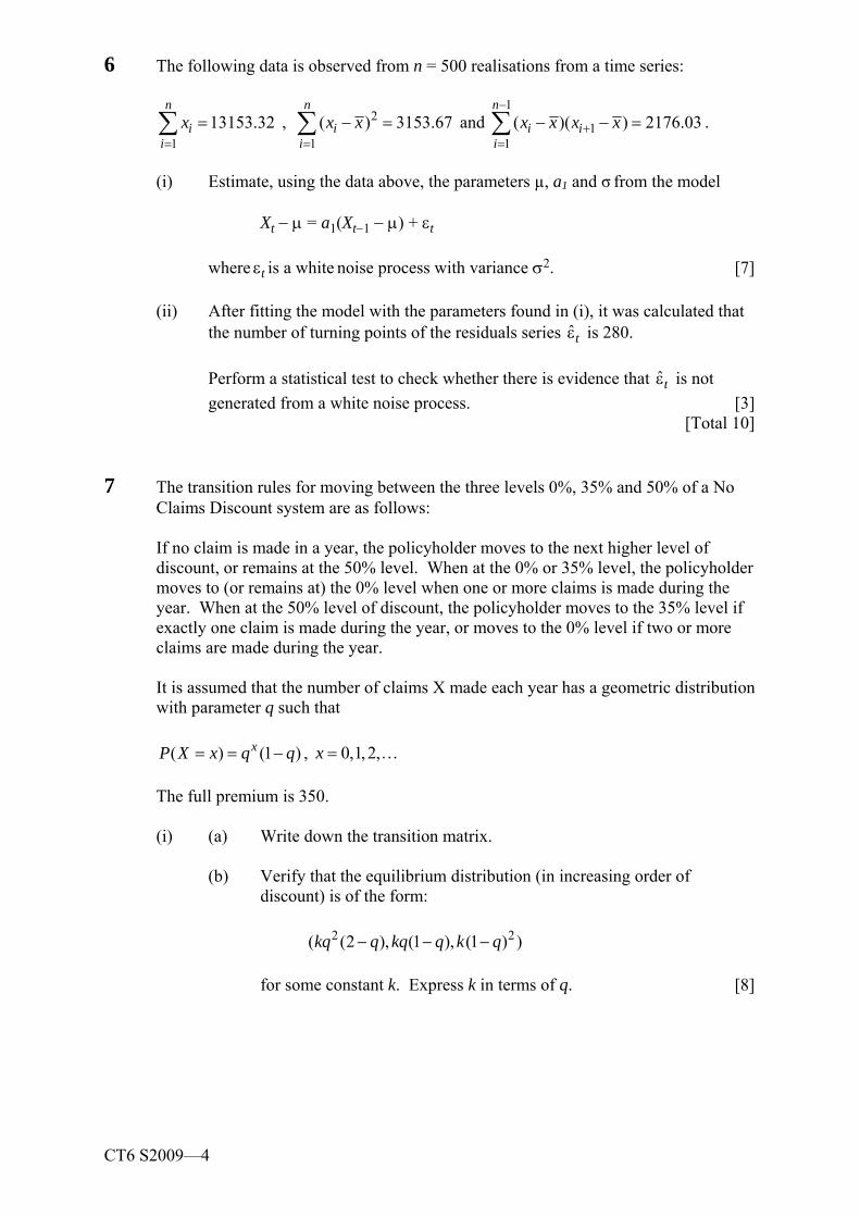
CT6 S2009—4
6 The following data is observed from n = 500 realisations from a time series:
113153.32
n
ii
x=
=∑ , 2
1( ) 3153.67
n
ii
x x=
− =∑ and 1
11
( )( ) 2176.03n
i ii
x x x x−
+=
− − =∑ .
(i) Estimate, using the data above, the parameters µ, a1 and σ from the model Xt − μ = a1(Xt−1 − μ) + εt where εt is a white noise process with variance σ2. [7]
(ii) After fitting the model with the parameters found in (i), it was calculated that the number of turning points of the residuals series ˆtε is 280.
Perform a statistical test to check whether there is evidence that ˆtε is not generated from a white noise process. [3]
[Total 10] 7 The transition rules for moving between the three levels 0%, 35% and 50% of a No
Claims Discount system are as follows: If no claim is made in a year, the policyholder moves to the next higher level of
discount, or remains at the 50% level. When at the 0% or 35% level, the policyholder moves to (or remains at) the 0% level when one or more claims is made during the year. When at the 50% level of discount, the policyholder moves to the 35% level if exactly one claim is made during the year, or moves to the 0% level if two or more claims are made during the year.
It is assumed that the number of claims X made each year has a geometric distribution
with parameter q such that ( ) (1 )xP X x q q= = − , 0,1,2,x = … The full premium is 350. (i) (a) Write down the transition matrix. (b) Verify that the equilibrium distribution (in increasing order of
discount) is of the form: 2 2( (2 ), (1 ), (1 ) )kq q kq q k q− − − for some constant k. Express k in terms of q. [8]

CT6 S2009—5 PLEASE TURN OVER
(ii) The value of the expected premium in the stationary state paid by “low risk” policyholders (with q = 0.05) is 178.51.
(a) Calculate the corresponding figure paid by “high risk” policyholders
(with q = 0.1). (b) Comment on the effectiveness of the No Claims Discount system.
[4] [Total 12] 8 The cumulative incurred claims for an insurance company for the last four accident
years are given in the following table: Development year
Accident year 0 1 2 3 2005 96 136 140 168 2006 100 156 160 2007 120 130 2008 136
It can be assumed that claims are fully run off after three years. The premiums
received for each year from 2005 to 2008 are 175, 181, 190 and 196 respectively. Calculate the reserve at the end of year 2008 using: (a) The basic chain ladder method. (b) The Bornhuetter-Ferguson method. [12]

CT6 S2009—6
9 A certain proportion p of electrical gadgets produced by a factory is defective. Prior beliefs about p are represented by a Beta distribution with parameters α and β. A sample of n gadgets is inspected, and k are found to be defective.
(i) Explain what is meant by a conjugate prior distribution. [1] (ii) Derive the posterior distribution for beliefs about p. [3]
(iii) Show that if X ~ Beta(α, β) with α > 1 then 1 11
EX
α +β−⎛ ⎞ =⎜ ⎟ α −⎝ ⎠. [3]
(iv) It is required to make an estimate d of p. The loss function is given by
2( )( , ) d pL d pp−
= .
Determine the Bayes estimate d* of p. [4] (v) Determine a parameter Z such that d* can be written as
d* 1(1 )kZ Zn
= × + − ×μ
where μ is the prior expectation of 1/p. [2]
(vi) Under quadratic loss, the Bayes estimate would have been kn
α +α +β+
.
Comment on the difference in the two Bayes’ estimates in the specific case where 3α = β = , k = 2 and n = 10. [2]
[Total 15]

CT6 S2009—7
10 The total number of claims N on a portfolio of insurance policies has a Poisson distribution with mean λ. Individual claim amounts are independent of N and each other, and follow a distribution X with mean μ and variance σ2. The total aggregate claims in the year is denoted by S. The random variable S therefore has a compound Poisson distribution.
(i) Derive an expression for the moment generating function of S in terms of the
moment generating function of X. [4] (ii) Derive expressions for the mean and variance of S in terms of λ, μ and σ. [6]
For a particular type of policy, individual losses are exponentially distributed with mean 100. For losses above 200 the insurer incurs an additional expense of 50 per claim.
(iii) Calculate the mean and variance of S for a portfolio of such policies with λ = 500. [9]
[Total 19]
END OF PAPER

Faculty of Actuaries
Institute of Actuaries
Faculty of Actuaries Institute of Actuaries
Subject CT6 — Statistical Methods.
Core Technical
September 2009 examinations
EXAMINERS’ REPORT
Introduction
The attached subject report has been written by the Principal Examiner with the aim of
helping candidates. The questions and comments are based around Core Reading as the
interpretation of the syllabus to which the examiners are working. They have however given
credit for any alternative approach or interpretation which they consider to be reasonable.
R D Muckart
Chairman of the Board of Examiners
December 2009
Comments for individual questions are given with the solutions that follow.

Subject CT6 (Statistical Methods Core Technical) — September 2009 — Examiners’ Report
Page 2
1
tY 12 t tY Z
12t tY Y tZ
(1 2 ) tB Y tZ
tY 1(1 2 ) tB Z
2 3(1 2 (2 ) (2 ) ) tB B B Z
0
(2 ) jt j
j
Z
So Var( )tY
0
Var (2 ) jt j
j
Z
2 2
0
(4 ) j
j
2
2(1 4 )
Other valid approaches to deriving the variance were given full credit.
This is a nice, short question involving time series. It requires a little knowledge about
series expansions, some algebraic manipulation and the formula for a geometric
progression. The question was answered reasonably well, with most candidates
recalling the series expansion for (1-X)-1
. Strong candidates spotted that the condition
|α|<0.5 was needed to use the formula for an infinite geometric series.
2
Let 1X denote aggregate claims in year 1, and let 2X denote aggregate claims in year
2. Then to avoid ruin after the first year, we require 1X <15 and to avoid ruin after 2
years we require 1X + 2X <30.
1 1 2( 15 and 30)P X X X 1
15
2
0
( ) ( 30 )Xf x P X x dx
150.1 0.1(30 )
0
0.1 (1 )x xe e dx
150.1 3
0
0.1 0.1xe e dx

Subject CT6 (Statistical Methods Core Technical) — September 2009 — Examiners’ Report
Page 3
15
0.1 3
00.1xe xe
1.5 31.5 1e e
0.702189
This was a question involving the concept of ruin in discrete time and requiring
candidates to calculate a probability by integrating the pdf of the exponential
distribution. This question was not answered well. Many candidates did not recognise
the condition for ruin at t=2, ie X1+X2<30.
3
(i) Decision 3d is dominated by 1d and can be discounted immediately.
(ii) Maximum losses are:
1d 15
2d 20
4d 23
So the minimax solution is to choose 1d
(iii) Expected losses are given by:
1
2
4
( ( )) 0.4 10 0.25 15 0.35 5 9.5
( ( )) 0.4 8 0.25 20 0.35 15 13.45
( ( )) 0.4 5 0.25 23 0.35 8 10.55
E L d
E L d
E L d
So the Bayes solution is also to choose 1d .
A straightforward question involving outcomes of 3 decision functions and requiring
the candidates to derive the minimax solution and the Bayes criterion solution. This
question was answered very well by most candidates.
4
(i) The likelihood is
12
1 1
(1 ) ij
ky
ij ij
i j
L
Where ijy is the number of claims on the ith policy in the jth month.
Taking the logarithm of L we have
12
)
1 1
log log log(1k
ij ij ij
i j
L y
and so
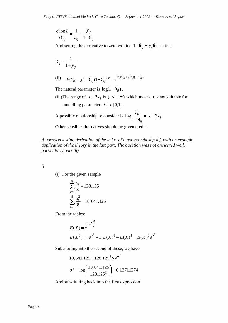
Subject CT6 (Statistical Methods Core Technical) — September 2009 — Examiners’ Report
Page 4
log 1
1
ij
ij ij ij
yL
And setting the derivative to zero we find ˆ ˆ1 ij ij ijy so that
1ˆ1
ijijy
(ii)
The natural parameter is log(1 )ij .
(iii) The range of jx is ( , ) which means it is not suitable for
modelling parameters [0,1]ij .
A possible relationship to consider is log1
ijj
ij
x .
Other sensible alternatives should be given credit.
A question testing derivation of the m.l.e. of a non-standard p.d.f, with an example
application of the theory in the last part. The question was not answered well,
particularly part iii).
5
(i) For the given sample
8
1
8 2
1
128.1258
18,641.1258
i
i
i
i
x
x
From the tables:
2
2 2
2
2 2 2 2
( )
( ) 1 ( ) ( ) ( )
E X e
E X e E X E X E X e
Substituting into the second of these, we have:
2218,641.125 128.125 e
2
2
18,641.125log 0.12711274
128.125
And substituting back into the first expression
log log(1 )( ) (1 ) ij ijyy
ij ij ijP Y y e

Subject CT6 (Statistical Methods Core Technical) — September 2009 — Examiners’ Report
Page 5
2
2128.125 e
2
log128.1252
log128.125 0.5 0.12711274 4.78945
(ii) The lower and upper quartile points in the data set are 95 and 168.5
We need to solve:
0.6745 0.6745168.5 and 95e e
Dividing the first by the second gives:
2 0.6745 1.773684211e
log1.7736842110.424802711
2 0.6745
2 0.180457343
And substituting back into the first equation:
0.6745 168.5e
log168.5 0.6745 0.424802711
4.840406
It is possible to use other definitions of upper and lower quartile. Other sensible
choices were given full credit provided the subsequent calculations followed
through correctly
A numerical question that tested the theory of fitting a distribution using two different
methods to sample data. This question was answered reasonably well, with some
candidates scoring very highly indeed. This question was a good differentiator with
strong candidates showing they had learnt the theory of distribution fitting thoroughly
and accurately calculating the answers. NB Both percentile definitions as per CT3
were given credit.
6
(i) Clearly 13153.32
ˆ 26.30644.500
Using the known expression of the auto covariance function for AR(1)
processes: k = 1 ,ka we see that

Subject CT6 (Statistical Methods Core Technical) — September 2009 — Examiners’ Report
Page 6
499
111 1 500 2
1
( )( ) 2176.03ˆ, 0.6899993
3153.67( )
i ik i
ii
x x x xa
x x
Taking the variance of both sides of
Xt = a1(Xt 1 ) + t
and using the fact that 0 = var(Xt ) = var(Xt 1 )
0 = 2 21 0 .a
Hence 2 2 2
0 1
3153.67ˆˆ (1 ( ) ) (1 0.6899993 ) 3.304416,
500a hat
i.e. ˆ 3.304416 1.817805
(ii) Using the fact that under the white noise assumptions the mean and
variance of the number of change points are
2( 2)
3
N
= 332 and
(16 29)
90
N
= 88.56667
respectively where N = 500. Therefore since the 95% confidence interval is
(332 1.96 88.56667,332 1.96 88.56667) (313.6,350.4)
which does not contain the observed number 280, there is a strong evidence
that the errors are not close to those of a white noise.
This was a slightly more complicated parameter fitting question for a time-series
model, and with a chi-square significance test to finish. The question was answered
poorly, with many candidates finding this one tough. Candidates scoring poorly for
part i) usually did not get ii) out as well.
7
(i)
a. Note first that
2
( 0) 1
( 1) (1 )
( 2) 1 (1 ) (1 )
( 1) 1 (1 )
P X q
P X q q
P X q q q q
P X q q

Subject CT6 (Statistical Methods Core Technical) — September 2009 — Examiners’ Report
Page 7
The transition matrix is
2
1 0
0 1
(1 ) 1
q q
P q q
q q q q
b. 2 21 2 3( (2 ), (1 ), (1 ) ) ( , , )kq q kq q k q P
Where
3 2 2 21
2 2
2 2 2
2
(2 ) (1 ) (1 )
(2 ) (1 ) (1 )
2 1 1 2
(2 )
kq q kq q kq q
kq q q q q
kq q q q q q
kq q
2 22
2
2 2
(2 )(1 ) (1 ) (1 )
(1 ) (2 ) (1 )
(1 )(2 1 2 )
(1 )
kq q q k q q q
kq q q q q
kq q q q q q
kq q
2 33
2
2
(1 ) (1 )
(1 ) ( 1 )
(1 )
kq q k q
k q q q
k q
Since the proportions must sum to 1, we have
2 2 2 3
1 1
(1 ) (1 ) (1 ) 2 1k
q q q q q q q q
(ii)
a. Average premium is:
L2 2
2 3
1350 0.1 1.9 0.65 0.1 0.9 0.5 0.9
2 0.1 0.1 0.1 1
= 183.76
b. Policyholders are twice as likely to claim, but the premium
increases only by 3%! Suggests that the NCD system is not
effective.
A 3x3 NCD problem with generic P(claim) = q, and P(not claim) = 1-q, and then a
numerical application. Despite some fiddly algebra, this question was based on
standard NCD theory and answered very well.
8
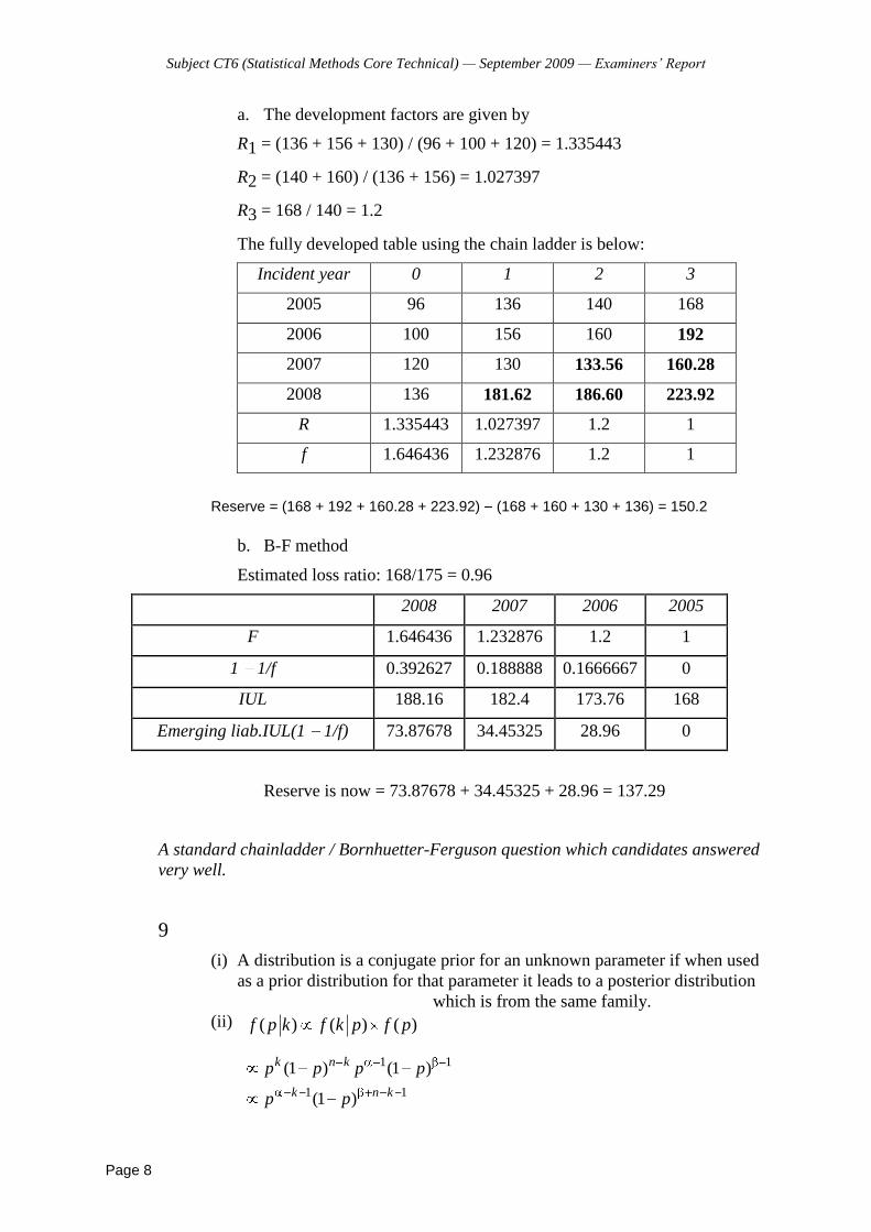
Subject CT6 (Statistical Methods Core Technical) — September 2009 — Examiners’ Report
Page 8
a. The development factors are given by
R1 = (136 + 156 + 130) / (96 + 100 + 120) = 1.335443
R2 = (140 + 160) / (136 + 156) = 1.027397
R3 = 168 / 140 = 1.2
The fully developed table using the chain ladder is below:
Incident year 0 1 2 3
2005 96 136 140 168
2006 100 156 160 192
2007 120 130 133.56 160.28
2008 136 181.62 186.60 223.92
R 1.335443 1.027397 1.2 1
f 1.646436 1.232876 1.2 1
Reserve = (168 + 192 + 160.28 + 223.92) (168 + 160 + 130 + 136) = 150.2
b. B-F method
Estimated loss ratio: 168/175 = 0.96
2008 2007 2006 2005
F 1.646436 1.232876 1.2 1
1 1/f 0.392627 0.188888 0.1666667 0
IUL 188.16 182.4 173.76 168
Emerging liab.IUL(1 1/f) 73.87678 34.45325 28.96 0
Reserve is now = 73.87678 + 34.45325 + 28.96 = 137.29
A standard chainladder / Bornhuetter-Ferguson question which candidates answered
very well.
9
(i) A distribution is a conjugate prior for an unknown parameter if when used
as a prior distribution for that parameter it leads to a posterior distribution
which is from the same family.
(ii)
( ) ( ) ( )f p k f k p f p
1 1
1 1
(1 ) (1 )
(1 )
k n k
k n k
p p p p
p p

Subject CT6 (Statistical Methods Core Technical) — September 2009 — Examiners’ Report
Page 9
Which is the pdf of a Beta( ,k n k ) distribution.
(iii)
Other derivations are acceptable.
(iv) Let
2 (1/ ) 2 ( )d E p d E p
And
When
Using the result from (iii) applied to the posterior distribution for p.
(v)
1 1 1*
1 1 1 1
(1 )
k k nd
n n n n
xZ Z
n
Where 1
nZ
n and is the prior expectation of 1/p.D
(vi) The estimates are:
Using the given loss function the estimate is
1E
X
11 1
0
1 ( )(1 )
( ) ( )x x dx
x
12 1
0
12 1
0
( )(1 )
( ) ( )
( 1) ( ) ( 1)(1 )
( ) ( 1) ( 1) ( )
( 1) ( 1) ( 1)1
( 1) ( 1) ( 1)
x x dx
x x dx
1.
1
( ) ( ( , ))h d E L d p
2 2 2( ) 2( )
d p d dp ph d E E
p p
( ) 2 (1/ ) 2h d dE p
( ) 0h d
2 * (1/ ) 2
1* 1/ (1/ )
1
d E p
kd E p
n
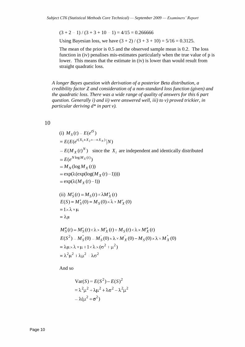
Subject CT6 (Statistical Methods Core Technical) — September 2009 — Examiners’ Report
Page 10
(3 + 2 1) / (3 + 3 + 10 1) = 4/15 = 0.266666
Using Bayesian loss, we have (3 + 2) / (3 + 3 + 10) = 5/16 = 0.3125.
The mean of the prior is 0.5 and the observed sample mean is 0.2. The loss
function in (iv) penalises mis-estimates particularly when the true value of p is
lower. This means that the estimate in (iv) is lower than would result from
straight quadratic loss.
A longer Bayes question with derivation of a posterior Beta distribution, a
credibility factor Z and consideration of a non-standard loss function (given) and
the quadratic loss. There was a wide range of quality of answers for this 6 part
question. Generally i) and ii) were answered well, iii) to v) proved trickier, in
particular deriving d* in part v).
10
(i) ( ) ( )tSSM t E e
1 2( )( ( )Nt X X X
E E e N
( ( ) )NXE M t since the iX are independent and identically distributed
log ( )( )XN M tE e
(log ( ))N XM M t
exp( (exp(log( ( ) 1))))XM t
exp( ( ( ) 1))XM t
(ii) ( ) ( ) ( )S S XM t M t M t
( ) (0) (0) (0)
1
S S XE S M M M
( ) ( ) ( ) ( ) ( )S S X S XM t M t M t M t M t
2 '' ' ' ''( ) (0) (0) (0) (0) (0)S S X S XE S M M M M M
2 2
2 2 2 2
1 ( )
And so
2 2
2 2 2 2 2 2
2 2
Var( ) ( ) ( )
( )
S E S E S

Subject CT6 (Statistical Methods Core Technical) — September 2009 — Examiners’ Report
Page 11
(iii) First, we must calculate the mean and variance of a single claim, say Y.
Let us denote by X the underlying loss. Then
( )E Y
2000.01 0.01
0 200
0.01 ( 50) 0.01x xxe dx x e dx
0.01 0.01
0 200
0.01 50 0.01x xxe dx e dx
( ) 50 ( 200)E X P X
= 200 0.01100 50 e
100 6.76676
106.76676
2002 2 0.01 2 0.01
0 200
( ) 0.01 ( 50) 0.01x xE Y x e dx x e dx
2 0.01 0.01 2 0.01
0 200 200
0.01 50 0.01x x xx e dx xe dx e dx
2 0.01 0.01 2
200200
( ) 100 100 50 ( 200)x xE X xe e d P X
2 2 2 2 0.01 2
200100 100 20,000 100 2,500xe e e
2 2 2
2
20,000 20,000 10,000 2,500
20,000 32,500
24,398.39671
e e e
e
And finally, using the results from part (ii)
( ) 500 ( ) 500 106.76676
53,383.38
E S E X
and
2Var( ) 500 ( ) 500 24,398.39671 12,199,198.36S E X
A long question about deriving mgf of a compound Poisson distribution. Mixture of
bookwork and proof, and a numerical application to finish. This question was
answered reasonably well, in particular part i) and part ii).
END OF EXAMINERS’ REPORT

Faculty of Actuaries Institute of Actuaries
EXAMINATION
20 April 2010 (am)
Subject CT6 — Statistical Methods Core Technical
Time allowed: Three hours
INSTRUCTIONS TO THE CANDIDATE
1. Enter all the candidate and examination details as requested on the front of your answer booklet.
2. You must not start writing your answers in the booklet until instructed to do so by the
supervisor. 3. Mark allocations are shown in brackets. 4. Attempt all 11 questions, beginning your answer to each question on a separate sheet. 5. Candidates should show calculations where this is appropriate.
Graph paper is NOT required for this paper.
AT THE END OF THE EXAMINATION
Hand in BOTH your answer booklet, with any additional sheets firmly attached, and this question paper.
In addition to this paper you should have available the 2002 edition of the Formulae and Tables and your own electronic calculator from the approved list.
© Faculty of Actuaries CT6 A2010 © Institute of Actuaries
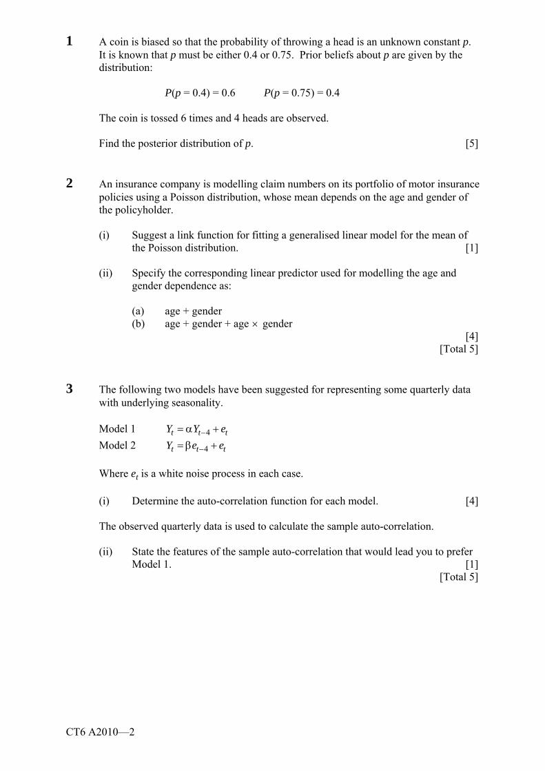
CT6 A2010—2
1 A coin is biased so that the probability of throwing a head is an unknown constant p. It is known that p must be either 0.4 or 0.75. Prior beliefs about p are given by the distribution:
P(p = 0.4) = 0.6 P(p = 0.75) = 0.4
The coin is tossed 6 times and 4 heads are observed.
Find the posterior distribution of p. [5] 2 An insurance company is modelling claim numbers on its portfolio of motor insurance
policies using a Poisson distribution, whose mean depends on the age and gender of the policyholder.
(i) Suggest a link function for fitting a generalised linear model for the mean of
the Poisson distribution. [1] (ii) Specify the corresponding linear predictor used for modelling the age and
gender dependence as: (a) age + gender (b) age + gender + age × gender
[4] [Total 5] 3 The following two models have been suggested for representing some quarterly data
with underlying seasonality.
Model 1 4t t tY Y e−= α + Model 2 4t t tY e e−= β +
Where et is a white noise process in each case.
(i) Determine the auto-correlation function for each model. [4] The observed quarterly data is used to calculate the sample auto-correlation. (ii) State the features of the sample auto-correlation that would lead you to prefer
Model 1. [1] [Total 5]

CT6 A2010—3 PLEASE TURN OVER
4 The number of claims N on a portfolio of insurance policies follows a binomial distribution with parameters n and p. Individual claim amounts follow an exponential distribution with mean 1/λ. The insurer has in place an individual excess of loss reinsurance arrangement with retention M.
(i) Derive an expression, involving M and λ, for the probability that an individual
claim involves the reinsurer. [2] Let Ii be an indicator variable taking the value 1 if the ith claim involves the reinsurer
and 0 otherwise. (ii) Evaluate the moment generating function ( )
iIM t . [1] Let K be the number of claims involving the re-insurer so that 1 NK I I= + + . (iii) (a) Find the moment generating function of K. (b) Deduce that K follows a binomial distribution with parameters that you
should specify. [4]
[Total 7] 5 An insurance company has issued life insurance policies to 1,000 individuals. Each
life has a probability q of dying in the coming year. In a warm year, q = 0.001 and in a cold year q = 0.005. The probability of a warm year is 50% and the probability of a cold year is 50%. Let N be the aggregate number of claims across the portfolio in the coming year.
(i) Calculate the mean and variance of N. [4] (ii) Calculate the alternative values for the mean and variance of N assuming that
q is a constant 0.003. [2] (iii) Comment on the results of (i) and (ii). [2] [Total 8]
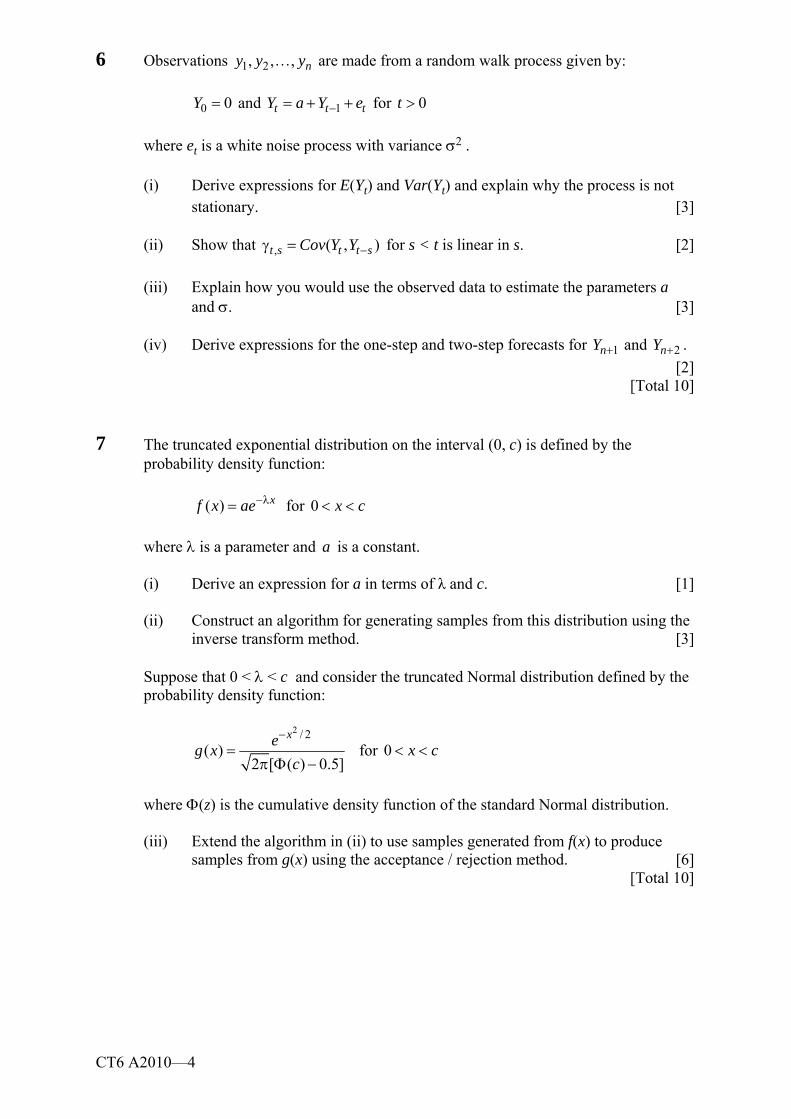
CT6 A2010—4
6 Observations 1 2, , , ny y y… are made from a random walk process given by:
0 0Y = and 1t t tY a Y e−= + + for 0t >
where et is a white noise process with variance σ2 . (i) Derive expressions for E(Yt) and Var(Yt) and explain why the process is not
stationary. [3] (ii) Show that , ( , )t s t t sCov Y Y −γ = for s < t is linear in s. [2] (iii) Explain how you would use the observed data to estimate the parameters a
and σ. [3] (iv) Derive expressions for the one-step and two-step forecasts for 1nY + and 2nY + .
[2] [Total 10] 7 The truncated exponential distribution on the interval (0, c) is defined by the
probability density function:
( ) xf x ae−λ= for 0 x c< <
where λ is a parameter and a is a constant. (i) Derive an expression for a in terms of λ and c. [1] (ii) Construct an algorithm for generating samples from this distribution using the
inverse transform method. [3] Suppose that 0 < λ < c and consider the truncated Normal distribution defined by the
probability density function:
2 / 2( )
2 [ ( ) 0.5]
xeg xc
−=
π Φ − for 0 x c< <
where Φ(z) is the cumulative density function of the standard Normal distribution.
(iii) Extend the algorithm in (ii) to use samples generated from f(x) to produce
samples from g(x) using the acceptance / rejection method. [6] [Total 10]
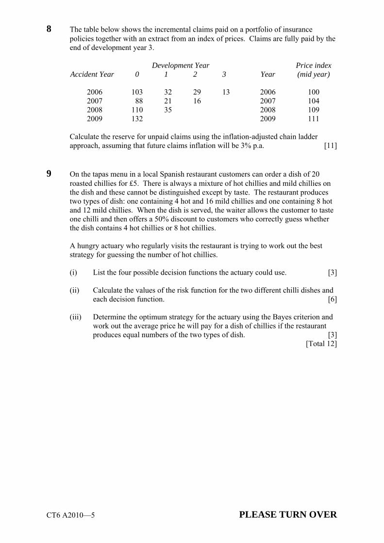
CT6 A2010—5 PLEASE TURN OVER
8 The table below shows the incremental claims paid on a portfolio of insurance policies together with an extract from an index of prices. Claims are fully paid by the end of development year 3.
Development Year Price index Accident Year
0 1 2 3 Year (mid year)
2006 103 32 29 13 2006 100 2007 88 21 16 2007 104 2008 110 35 2008 109 2009 132 2009 111
Calculate the reserve for unpaid claims using the inflation-adjusted chain ladder
approach, assuming that future claims inflation will be 3% p.a. [11] 9 On the tapas menu in a local Spanish restaurant customers can order a dish of 20
roasted chillies for £5. There is always a mixture of hot chillies and mild chillies on the dish and these cannot be distinguished except by taste. The restaurant produces two types of dish: one containing 4 hot and 16 mild chillies and one containing 8 hot and 12 mild chillies. When the dish is served, the waiter allows the customer to taste one chilli and then offers a 50% discount to customers who correctly guess whether the dish contains 4 hot chillies or 8 hot chillies.
A hungry actuary who regularly visits the restaurant is trying to work out the best
strategy for guessing the number of hot chillies. (i) List the four possible decision functions the actuary could use. [3] (ii) Calculate the values of the risk function for the two different chilli dishes and
each decision function. [6] (iii) Determine the optimum strategy for the actuary using the Bayes criterion and
work out the average price he will pay for a dish of chillies if the restaurant produces equal numbers of the two types of dish. [3]
[Total 12]

CT6 A2010—6
10 Claims on a portfolio of insurance policies arrive as a Poisson process with annual rate λ. Individual claims are for a fixed amount of 100 and the insurer uses a premium loading of 15%. The insurer is considering entering a proportional reinsurance agreement with a reinsurer who uses a premium loading of 20%. The insurer will retain a proportion α of each risk.
(i) Write down and simplify the equation defining the adjustment coefficient R
for the insurer. [3] (ii) By considering R as a function of α and differentiating show that
100(120 5) 120 100 100 RdR dRR R ed d
α⎛ ⎞α − + = + α⎜ ⎟α α⎝ ⎠ [3]
(iii) Explain why setting dRdα
= 0 and solving for α may give an optimal value
for α. [3] (iv) Use the method suggested in part (iii) to find an optimal choice for α. [4] [Total 13]

CT6 A2010—7
11 An actuary has, for three years, recorded the volume of unsolicited advertising that he receives. He believes that the number of items that he receives follows a Poisson distribution with a mean which varies according to which quarter of the year it is. He has recorded Yij the number of items received in the ith quarter of the jth year (i = 1, 2, 3, 4 and j = 1, 2, 3). The actuary wishes to estimate the number of items that he will receive in the 1st quarter of year 4. He has recorded the following data:
1iY
2iY 3iY 13i ij
jY Y= ∑ ( )2ij i
jY Y−∑
i = 1 98 117 124 113 362 i = 2 82 102 95 93 206 i = 3 75 83 88 82 86 i = 4 132 152 148 144 224
(i) Estimate Y1,4 the number of items that the actuary expects to receive in the
first quarter of year 4 using the assumptions of EBCT model 1. [5] The actuary believes that, in fact, the volume of items has been increasing at the rate
of 10% per annum. (ii) Suggest how the approach in (i) can be adjusted to produce a revised estimate
taking this growth into account. [2] (iii) Calculate the maximum likelihood estimate of Y1,4 (based on the quarter 1 data
already observed and the 10% p.a. increase described above). [5] (iv) Compare the assumptions underlying the approach in (i) and (ii) with those
underlying the approach in (iii). [2] [Total 14]
END OF PAPER

Faculty of Actuaries Institute of Actuaries
EXAMINERS REPORT
April 2010 examinations
Subject CT6 — Statistical Methods Core Technical
Introduction The attached subject report has been written by the Principal Examiner with the aim of helping candidates. The questions and comments are based around Core Reading as the interpretation of the syllabus to which the examiners are working. They have however given credit for any alternative approach or interpretation which they consider to be reasonable. R D Muckart Chairman of the Board of Examiners July 2010
Comments These are given in italics at the end of each question. © Faculty of Actuaries © Institute of Actuaries

Subject CT6 (Statistical Methods Core Technical) — April 2010 — Examiners’ Report
Page 2
1 (4 0.4) ( 0.4)( 0.4 4 )
(4 )P H p P p
P p HP H= =
= =
But P(4H) = (4 0.4) ( 0.4) (4 0.75) ( 0.75)P H p P p P H p P p= = + = =
= 4 2 4 26 60.4 0.6 0.6 0.75 0.25 0.4
4 4⎛ ⎞ ⎛ ⎞
× + ×⎜ ⎟ ⎜ ⎟⎝ ⎠ ⎝ ⎠
= 0.082944 + 0.11865 = 0.201596
So 0.082944( 0.4 4 ) 0.4114360.201596
P p H= = =
So the posterior distribution of p is given by P(p = 0.4) = 0.411436 and P(p = 0.75) = 0.588564 Comment: This question was intended to be a straightforward application of Bayes’ Theorem. However, the question was generally not well answered, with many candidates unable to find the posterior distribution in this slightly unfamiliar scenario. 2 (i) The link function here is ( ) logg μ = μ . (ii) (a) The linear predictor is i xα +β where the intercept iα for 1, 2i =
depends on gender. (b) The linear predictor is i i xα +β so that both parameters depend on
gender. Comment: This straightforward question was generally well answered. 3 (i) Model 1 In general we have 4k k−γ = αγ Taking covariance with 1 2 3, , ,t t t tY Y Y Y− − − we get: 1 3γ = αγ 2 2γ = αγ 3 1γ = αγ For 0α ≠ these equations imply that 0kρ = unless k is divisible by 4.
Subject CT6 (Statistical Methods Core Technical) — April 2010 — Examiners’ Report
Page 3
So we have 4k
kρ = α and all other autocorrelations are zero. Model 2 Here we have 0kγ = unless k=4 and k=0. In these cases . So 0 1ρ = , and all the other autocorrelations are zero. (ii) Model 1 is preferred in situations where the sample auto-correlation is non-
zero and decays exponentially. Comment: This question was reasonably well attempted, although a number of candidates dropped marks especially in calculating the ACF of Model 1. 4 (i) Let X represent the distribution of individual claims. Let denote the
probability that an individual claim involves the reinsurer. Then
π = ( ) x
M
P X M e dx∞
−λ> = λ∫
= xM
e∞−λ⎡ ⎤−⎣ ⎦
= Me−λ (ii) ( ) ( ) 1i
itI t
IM t E e e= = π + −π (iii) Using the results for the moment generating function of a compound
distribution, we have ( )KM t = (log ( ))
iN IM M t
= ( )( ) 1i
nIpM t p+ −
= ( )( 1 ) 1ntp e pπ + −π + −
= ( )1ntp e p p pπ + − π+ −
Subject CT6 (Statistical Methods Core Technical) — April 2010 — Examiners’ Report
Page 4
= ( )1ntp e pπ + − π
Which is the MGF of a binomial distribution with parameters n and pπ . Hence, by the uniqueness of MGFs K has a binomial distribution with
parameters n and pπ . Comment: This question was well answered. 5 (i) ( )E N = ( )E E N q⎡ ⎤⎣ ⎦ = [ ]1000E q
= ( )1000 0.5 0.001 0.5 0.005× × + × = 1000 0.003 3× = ( )Var N = ( )( )Var E N q E Var N q⎡ ⎤⎡ ⎤ +⎣ ⎦ ⎣ ⎦
= (1000 ) (1000 (1 ))Var q E q q+ − Now ( ) 0.003E q = and 2 2 2( ) 0.5 0.001 0.5 0.005 0.000013E q = × + × = So 2( ) 0.000013 0.003 0.000004Var q = − = ( (1 )) 0.5 0.001 0.999 0.5 0.005 0.995 0.002987E q q− = × × + × × = So 2( ) 1000 0.000004 1000 0.002987 6.987Var N = × + × = (ii) In this case ~ (1000,0.003)N B and so ( ) 1000 0.003 3E N = × = and ( ) 1000 0.003 0.997 2.991Var N = × × = (iii) The simplification in (ii) results in the same mean number of deaths, but a
very significantly lower variance.
Subject CT6 (Statistical Methods Core Technical) — April 2010 — Examiners’ Report
Page 5
This is because in (i) there is a tendency for deaths to occur at the same time, or not at all (as a result of the weather) whereas in (ii) deaths are genuinely independent.
Comment: Many good answers here although some candidates struggled to articulate why the variance in (ii) was lower.
6 (i) We can deduce that 1
t
t ii
Y at e=
= +∑
and so ( )tE Y at= and
2( )tVar Y t= σ . Since these expressions depend on t the process is not stationary. (ii) As s < t we have
2
1 1 1( , ) ( , ) ( ) ( )
t t s t s
t t s i j ji j j
Cov Y Y Cov at e as e Var e t s− −
−= = =
= + + = = − σ∑ ∑ ∑
Which is linear in s as required. (iii) First note that the differenced series: 1t t t tX Y Y a e−= − = + is essentially a white noise process. So estimates of a and 2σ can be found by
constructing the sample differences series 1i i ix y y −= − for 1, 2, ,i n= … and taking the mean and sample variance(or its square for estimating ) respectively.
(iv) In this case ˆ ˆ ˆ(1) 0n n ny a y a y= + + = + And ˆ ˆ ˆ ˆ(2) (1) 0 2n n ny a y a y= + + = + Comment: This was a rather hard question with many candidates confirming the non-stationarity in (i) but not finding the general solution. In part (ii) a good number of answers failed to score full marks. Alternative answers to (i) and (ii) could have been obtained by increasing t iteratively and noticing a pattern developing.

Subject CT6 (Statistical Methods Core Technical) — April 2010 — Examiners’ Report
Page 6
7 (i) ( )00
1 1c c
x x ca aae dx e e−λ −λ −λ⎡ ⎤= = − = −⎢ ⎥λ λ⎣ ⎦∫
So 1 ca
e−λλ
=−
(ii) The distribution function is
( )F x =00
x xy yaae dy e−λ −λ⎡ ⎤= −⎢ ⎥λ⎣ ⎦∫
= ( ) 111
xx
ca ee
e
−λ−λ
−λ−
− =λ −
The required transformation is therefore given by:
( )log 1 (1 )
( ) 1 (1 )c
x cu e
u F x e u e x− λ
−λ −λ− −
= ⇔ − = − ⇔ = −λ
So the algorithm is:
• Generate u from U(0, 1)
• Set ( )log 1 (1 )cu e
x− λ− −
= −λ
(iii) We need to find 2 / 2
0 0
( ) (1 )( ) 2 [ ( ) 0.5]
c x x
x c x c
g x e eMf x cMax Max
− λ − +λ
< < < <
−= =
π Φ − λ
Let
2 /2( ) x xh x e− +λ= then we can simply find the maximum of h(x) since it differs only by a constant.
Then '( ) ( ) ( )h x h x x= × − + λ So '( ) 0h x = when x = λ ''( ) '( )( ) ( )h x h x x h x= λ − − And so ''( ) ( ) 0h hλ = − λ < so we do have a maximum.
Hence 2 / 2(1 )
2 [ ( ) 0.5]
ce eMc
− λ λ−=
π Φ − λ

Subject CT6 (Statistical Methods Core Technical) — April 2010 — Examiners’ Report
Page 7
And so 2 2/2 /2( )
( )x xg x e
Mf x− +λ −λ=
So the algorithm is:
• Generate u from U(0,1)
• Set ( )log 1 (1 )cu e
x− λ− −
= −λ
• Generate v from U(0,1)
• If 2 2/2 /2x xv e− +λ −λ< return x as the random sample, otherwise begin again.
Comment: This was found particularly hard especially part (iii), where some harder calculations are involved. Many candidates just described the general theory of rejection algorithms without being able to apply it explicitly here. 8 (i) Adjusting the incremental data for inflation to mid 2008 prices gives:
Development Year Accident Year
0 1 2 3
2006 114.3 34.2 29.5 13 2007 93.9 21.4 16 2008 112.0 35 2009 132
Cumulating gives
Development Year Accident Year
0 1 2 3
2006 114.3 148.5 178.0 191.0 2007 93.9 115.3 131.3 2008 112.0 147.0 2009 132.0
The development factors are:
Year 0 to year 1 148.5 115.3 147.0 1.2827114.3 93.9 112.0
+ +=
+ +
Year 1 to year 2 178.0 131.3 1.1726148.5 115.3
+=
+
Subject CT6 (Statistical Methods Core Technical) — April 2010 — Examiners’ Report
Page 8
Year 2 to year 3 191.0 1.0730178.0
=
The completed table at mid 2008 prices is:
Development Year Accident Year
0 1 2 3
2006 2007 140.9 2008 172.4 185.0 2009 169.3 198.5 213.0
Differencing gives:
Development Year Accident Year 0 1 2 3
2006 2007 9.6 2008 25.4 12.6 2009 37.3 29.2 14.5
And so the total reserve is 2 3(37.3 25.4 9.6) 1.03 (29.2 12.6) 1.03 14.5 1.03 134.7+ + × + + × + × = Comment: This was a straightforward question with many candidates scoring full marks here. 9 (i) The possibilities are (where H denotes trying a hot chilli and M denotes trying
a mild chilli) 1 1( ) 4 and ( ) 4d H H d M H= = 2 2( ) 4 and ( ) 8d H H d M H= = 3 3( ) 8 and ( ) 4d H H d M H= = 4 4( ) 8 and ( ) 8d H H d M H= = (ii) Under 4H we have ( ) 0.2P H = and ( ) 0.8P M = Under 8H we have ( ) 0.4P H = and ( ) 0.6P M =
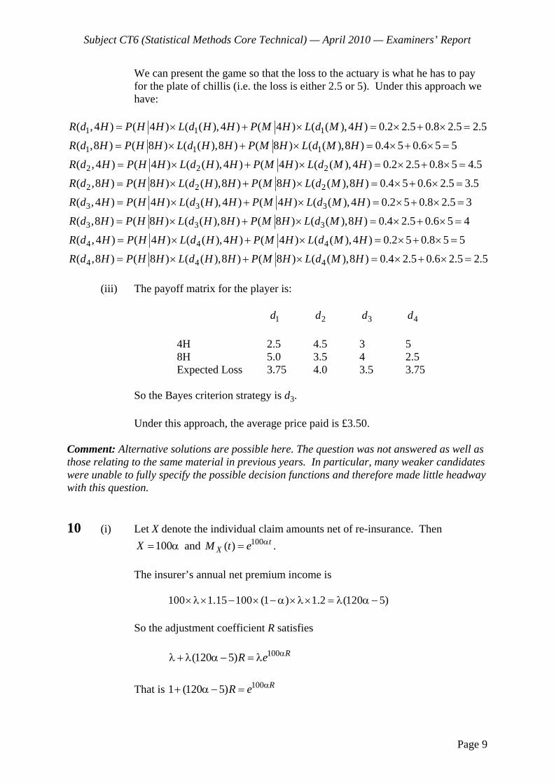
Subject CT6 (Statistical Methods Core Technical) — April 2010 — Examiners’ Report
Page 9
We can present the game so that the loss to the actuary is what he has to pay for the plate of chillis (i.e. the loss is either 2.5 or 5). Under this approach we have:
1 1 1( ,4 ) ( 4 ) ( ( ), 4 ) ( 4 ) ( ( ), 4 ) 0.2 2.5 0.8 2.5 2.5R d H P H H L d H H P M H L d M H= × + × = × + × = 1 1 1( ,8 ) ( 8 ) ( ( ),8 ) ( 8 ) ( ( ),8 ) 0.4 5 0.6 5 5R d H P H H L d H H P M H L d M H= × + × = × + × =
2 2 2( , 4 ) ( 4 ) ( ( ), 4 ) ( 4 ) ( ( ), 4 ) 0.2 2.5 0.8 5 4.5R d H P H H L d H H P M H L d M H= × + × = × + × =
2 2 2( ,8 ) ( 8 ) ( ( ),8 ) ( 8 ) ( ( ),8 ) 0.4 5 0.6 2.5 3.5R d H P H H L d H H P M H L d M H= × + × = × + × =
3 3 3( , 4 ) ( 4 ) ( ( ), 4 ) ( 4 ) ( ( ), 4 ) 0.2 5 0.8 2.5 3R d H P H H L d H H P M H L d M H= × + × = × + × =
3 3 3( ,8 ) ( 8 ) ( ( ),8 ) ( 8 ) ( ( ),8 ) 0.4 2.5 0.6 5 4R d H P H H L d H H P M H L d M H= × + × = × + × =
4 4 4( , 4 ) ( 4 ) ( ( ), 4 ) ( 4 ) ( ( ), 4 ) 0.2 5 0.8 5 5R d H P H H L d H H P M H L d M H= × + × = × + × =
4 4 4( ,8 ) ( 8 ) ( ( ),8 ) ( 8 ) ( ( ),8 ) 0.4 2.5 0.6 2.5 2.5R d H P H H L d H H P M H L d M H= × + × = × + × =
(iii) The payoff matrix for the player is:
1d
2d 3d 4d
4H 2.5 4.5 3 5 8H 5.0 3.5 4 2.5 Expected Loss 3.75 4.0 3.5 3.75
So the Bayes criterion strategy is d3. Under this approach, the average price paid is £3.50. Comment: Alternative solutions are possible here. The question was not answered as well as those relating to the same material in previous years. In particular, many weaker candidates were unable to fully specify the possible decision functions and therefore made little headway with this question. 10 (i) Let X denote the individual claim amounts net of re-insurance. Then
100X = α and 100( ) tXM t e α= .
The insurer’s annual net premium income is 100 1.15 100 (1 ) 1.2 (120 5)×λ× − × −α ×λ× = λ α − So the adjustment coefficient R satisfies 100(120 5) RR e αλ +λ α − = λ That is 1001 (120 5) RR e α+ α− =
Subject CT6 (Statistical Methods Core Technical) — April 2010 — Examiners’ Report
Page 10
(ii) Differentiating this equation with respect to α we get
100120 (120 5) RdR dR ed d
α⎡ ⎤+ α − = ⎣ ⎦α α
and 100 Rd ed
α⎡ ⎤⎣ ⎦α
= [ ]100 100R de Rd
α αα
= 100 100 100R dRe Rd
α ⎛ ⎞+ α⎜ ⎟α⎝ ⎠
So putting these together, we have:
100(120 5) 120 100 100 RdR dRR R ed d
α⎛ ⎞α − + = + α⎜ ⎟α α⎝ ⎠
(iii) Firstly, by Lundberg’s inequality the higher the value of R the lower the upper
bound on the probability of ruin. So we wish to choose α so that R is a maximum.
That is, we need 0dRd
=α
.
(iv) Putting 0dRd
=α
in the equation in (ii) we get
100120 100Re RR α= i.e. 100 1.2Re α =
i.e. log1.2100
R =α
substituting into the equation in (i) gives
log1.21 (120 5) 1.2100
+ α − × =α
i.e. 100 (120 5) log1.2 120α + α − = α 20 120 log1.2 5log1.2− α + α =
So 5log1.2 0.48526120log1.2 20
α = =−
Subject CT6 (Statistical Methods Core Technical) — April 2010 — Examiners’ Report
Page 11
Comment: This question on material new to the syllabus for 2010 was not answered well with many candidates struggling, especially in the last part.
11 (i) The overall mean is given by 113 93 82 144 1084
Y + + += =
( )2( )E s θ = 4 3
2
1 1
1 1 362 206 86 224( ) 109.754 2 8ij i
i jY Y
= =
⎛ ⎞ + + +⎜ ⎟− = =⎜ ⎟⎝ ⎠
∑ ∑
( ( ))Var m θ = ( )24
2
1
1 1 ( ( ))3 3i
iY Y E S
=− − θ∑
= 2 2 2 2(113 108) (93 108) (82 108) (144 108) 109.75
3 3− + − + − + −
−
= 704.083
So the credibility factor is 3 0.950608109.753704.083
Z = =+
And the estimate for next quarter is 0.950608 113 (1 0.950608) 108 112.75× + − × = (ii) The average number of pieces of mail is assumed to be growing each year.
We need to adjust the data to take account of this. Two approaches are:
• Convert the data into “Year 4” values by increasing by 10% p.a. and then applying the methodology above; OR
• Recognise the lower volume of data in earlier years, by applying a risk
volume to each year and using EBCT model 2. If the risk volume for year 4 is 1, then the risk volume for year 3 is 1/1.1 and year 2 is 1/1.21 etc.
(iii) Let the mean number of items in quarter 1 of year 1 be given by λ . Then the
likelihood is given by:
21311 121.1 1.1 2(1.1 ) (1.1 )YY YL e e e−λ − λ − λ∝ λ λ λ
And so the log likelihood is 2
11 12 13log (1 1.1 1.1 ) ( ) logl L C Y Y Y= = −λ + + + + + λ

Subject CT6 (Statistical Methods Core Technical) — April 2010 — Examiners’ Report
Page 12
Differentiating 2 11 12 13(1 1.1 1.1 ) Y Y Yl + +∂= − + + +
∂λ λ
And setting this equal to zero gives:
11 12 132
98 117 124ˆ 102.4173.311 1.1 1.1
Y Y Y+ + + +λ = = =
+ +
So the estimate for Q1 in year 4 is 3 ˆ1.1 1.331 102.417 136.32×λ = × = (iv) The main difference is that the maximum likelihood estimate approach
considers the data for Q1 in isolation, whereas the EBCT approach assumes that data from other quarters come from a related distribution and so can tell us something about Q1.
Specifically, the EBCT approach assumes that the mean volume of unsolicited
mail for each quarter is itself a sample from a common distribution. Hence whilst each quarter has a different mean, they provide some information about the population from which the mean is drawn.
Comment: The same comment as in the previous question is valid here. This question was not very well answered question but with various alternative answers in (ii) and (iv).
END OF EXAMINERS’ REPORT

Faculty of Actuaries Institute of Actuaries
EXAMINATION
30 September 2010 (am)
Subject CT6 — Statistical Methods Core Technical
Time allowed: Three hours
INSTRUCTIONS TO THE CANDIDATE
1. Enter all the candidate and examination details as requested on the front of your answer booklet.
2. You must not start writing your answers in the booklet until instructed to do so by the
supervisor. 3. Mark allocations are shown in brackets. 4. Attempt all 11 questions, beginning your answer to each question on a separate sheet. 5. Candidates should show calculations where this is appropriate.
Graph paper is NOT required for this paper.
AT THE END OF THE EXAMINATION
Hand in BOTH your answer booklet, with any additional sheets firmly attached, and this question paper.
In addition to this paper you should have available the 2002 edition of the Formulae and Tables and your own electronic calculator from the approved list.
© Faculty of Actuaries CT6 S2010 © Institute of Actuaries
CT6 S2010—2
1 An actuary is using a simulation technique to estimate the probability θ that a claim on an insurance policy exceeds a given amount. The actuary has carried out 50 simulations and has produced an estimate that ˆ 0.47θ = . The variance of the simulated values is 0.15.
Calculate the minimum number of simulations that the actuary will have to perform in
order to estimate θ to within 0.01 with 95% confidence. [4] 2 Claims on a portfolio of insurance policies follow a compound Poisson process with
annual claim rate λ. Individual claim amounts are independent and follow an exponential distribution with mean μ. Premiums are received continuously and are set using a premium loading of θ. The insurer’s initial surplus is U.
Derive an expression for the adjustment coefficient, R, for this portfolio in terms of μ
and θ. [4] 3 An underwriter has suggested that losses on a certain class of policies follow a
Weibull distribution. She estimates that the 10th percentile loss is 20 and the 90th percentile loss is 95.
(i) Calculate the parameters of the Weibull distribution that fit these percentiles.
[3] (ii) Calculate the 99.5th percentile loss. [2] [Total 5] 4 An office worker receives a random number of e-mails each day. The number of
emails per day follows a Poisson distribution with unknown mean μ. Prior beliefs about μ are specified by a gamma distribution with mean 50 and standard deviation 15. The worker receives a total of 630 e-mails over a period of ten days.
Calculate the Bayesian estimate of μ under all or nothing loss. [7]
CT6 S2010—3 PLEASE TURN OVER
5 The table below shows aggregate annual claim statistics for three risks over a period of seven years. Annual aggregate claims for risk i in year j are denoted by Xij.
Risk, i
7
1
17i ij
jX X
=
= ∑
( )
272
1
16i ij i
jS X X
=
= −∑
i = 1 127.9 335.1 i = 2 88.9 65.1 i = 3 149.7 33.9
(i) Calculate the credibility premium of each risk under the assumptions of EBCT
Model 1. [6] (ii) Explain why the credibility factor is relatively high in this case. [2] [Total 8] 6 The probability density function of a gamma distribution is given in the following
parameterised form:
1( )( )
x
f x x eαα −
α− μαα
=μ Γ α
for x > 0.
(i) Express this density in the form of a member of the exponential family,
specifying all the parameters. [6] (ii) Hence show that the mean and variance of the distribution are given by μ and
2μα
respectively. [3]
[Total 9] 7 An insurance company has a portfolio of policies under which individual loss
amounts follow an exponential distribution with mean 1/λ. There is an individual excess of loss reinsurance arrangement in place with retention level 100. In one year, the insurer observes:
• 85 claims for amounts below 100 with mean claim amount 42; and • 39 claims for amounts above the retention level.
(i) Calculate the maximum likelihood estimate of λ. [5] (ii) Show that the estimate of λ produced by applying the method of moments to
the distribution of amounts paid by the insurer is 0.011164. [5] [Total 10]
CT6 S2010—4
8 Claims on a portfolio of insurance policies arrive as a Poisson process with rate λ. The claim sizes are independent identically distributed random variables X1, X2, …with:
( )i kP X k p= = for 1, 2, ,k M= … and 1
1M
kk
p=
=∑ .
The premium loading factor is θ. (i) Show that the adjustment coefficient R satisfies:
1
2
21 log(1 ) mRM m
θ+ θ < <
where 1( )i
im E X= for 1, 2i = . [7]
[The inequality 1Rx RMx xe eM M
≤ + − for 0 x M≤ ≤ may be used without
proof.] (ii) (a) Determine upper and lower bounds for R if θ = 0.3 and Xi is equally
likely to be 2 or 3 (and cannot take any other values). (b) Hence derive an upper bound on the probability of ruin when the initial
surplus is U. [3] [Total 10] 9 An actuarial student has been working on some claims projections but some of her
workings have been lost. The cumulative claim amounts and projected ultimate claims are given by the following table:
Accident Development Year Ultimate
Year 0 1 2 3
1 1001 1485 1762 W X 2 1250 Y 1820 1862.3 3 1302 1805 2122.5 4 Z 2278.8
All claims are paid by the end of development year 3. It is known that ultimate claims for accident years 2 and 3 have been estimated using
the Basic Chain Ladder method. (i) Calculate the values of W, X and Y. [5] For accident year 4 the student has used the Bornhuetter-Ferguson method using an
earned premium of 2,500 and an expected loss ratio of 90%.
CT6 S2010—5 PLEASE TURN OVER
(ii) Calculate the value of Z. [4] (iii) Calculate the outstanding claims reserve for all accident years implied by the
completed table. [1] [Total 10] 10 An insurance company has a portfolio of 10,000 policies covering buildings against
the risk of flood damage. (i) State the conditions under which the annual number of claims on the portfolio
can be modelled by a binomial distribution B(n, p) with n = 10,000. [3] These conditions are satisfied and p = 0.03. Individual claim amounts follow a
normal distribution with mean 400 and standard deviation 50. The insurer wishes to take out proportional reinsurance with the retention α set such that the probability of aggregate payments on the portfolio after reinsurance exceeding 120,000 is 1%.
(ii) Calculate α assuming that aggregate annual claims can be approximated by a
normal distribution. [7] This reinsurance arrangement is set up with a reinsurer who uses a premium loading
of 15%. (iii) Calculate the annual premium charged by the reinsurer. [2] As an alternative, the reinsurer has offered an individual excess of loss reinsurance
arrangement with a retention of M for the same annual premium. The reinsurer uses the same 15% loading to calculate premiums for this arrangement.
(iv) Show that the retention M is approximately 358.50. [4] [You may wish to use the following formula which is given on page 18 of the Tables: If f(x) is the PDF of the N(μ, σ2) distribution then
[ ] [ ]( ) ( ') ( ') ( ') ( ')U
Lxf x dx U L U L= μ Φ −Φ −σ ϕ −ϕ∫
where ' LL −μ=
σ and ' UU −μ
=σ
.
Here Φ(z) is the cumulative density function of the N(0, 1) distribution and
2
2( )
2
z
ez−
ϕ =π
.] [Total 16]

CT6 S2010—6
11 A time series model is specified by
21 22t t t tY Y Y e− −= α −α +
where et is a white noise process with variance σ2.
(i) Determine the values of α for which the process is stationary. [2] (ii) Derive the auto-covariances γ0 and γ1 for this process and find a general
recursive expression for γk for k ≥ 2. [10] (iii) Show that the auto-covariance function can be written in the form: k k
k A kBγ = α + α for some values of A, B which you should specify in terms of the constants α
and σ2. [5] [Total 17]
END OF PAPER
INSTITUTE AND FACULTY OF ACTUARIES
EXAMINERS’ REPORT
September 2010 examinations
Subject CT6 — Statistical Methods Core Technical
Introduction The attached subject report has been written by the Principal Examiner with the aim of helping candidates. The questions and comments are based around Core Reading as the interpretation of the syllabus to which the examiners are working. They have however given credit for any alternative approach or interpretation which they consider to be reasonable. T J Birse Chairman of the Board of Examiners December 2010
© Institute and Faculty of Actuaries
Subject CT6 (Statistical Methods Core Technical) — September 2010 — Examiners’ Report
Page 2
1 We know that, approximately, 2ˆ (0, )N nτθ −θ ≈ where 2τ can be approximated by
0.15.
Then ˆ
1.96 1.96 0.950.15
Pn
⎡ ⎤θ −θ⎢ ⎥− ≤ ≤ =⎢ ⎥
⎢ ⎥⎣ ⎦
And we require 0.151.96 0.01n
× ≤
That is 2
21.96 0.15 5762.4
0.01n ×≥ = i.e. n must be at least 5763
This question was generally poorly answered. 2 The adjustment coefficient satisfies the equation:
(1 ) ( )XR M Rλ + λμ + θ = λ
Where X is exponentially distributed with mean μ so that 1/ 1( )1/ 1XM t
t tμ
= =μ − −μ
So we have 11 (1 )1
RR
+μ + θ =−μ
and so 1 (1 )(1 ) 1R R R−μ + μ + θ −μ =
2 2(1 ) 0R R R R−μ +μ +μθ −μ +θ =
Dividing through by Rμ gives
(1 )Rμ + θ = θ
So (1 )
R θ=μ + θ
.
This question was well answered by most candidates.
Subject CT6 (Statistical Methods Core Technical) — September 2010 — Examiners’ Report
Page 3
3 (i) Let the parameters be c and γ as per the tables. Then we have:
201 0.1ceγ− ×− = so 20 0.9ce
γ− × = and so 20 log 0.9c γ× = − (A) And similarly 95 log 0.1c γ× = − (B)
(A) divided by (B) gives 20 log 0.9 0.045757595 log 0.1
γ⎛ ⎞ = =⎜ ⎟⎝ ⎠
So log 0.0457575 1.979533720log95
γ = =⎛ ⎞⎜ ⎟⎝ ⎠
And substituting into (A) we have 1.9795337log 0.9 0.000280056
20c = − =
(ii) The 99.5th percentile loss is given by
1.97953370.002800561 0.995xe−− =
So that 1.97953370.000280056 log 0.005x− =
log 0.005log0.000280056log 4.97486366
1.9795337x
⎛ ⎞⎜ ⎟−⎝ ⎠= =
So 4.97486366 144.73x e= = Most candidates scored well on this question. 4 Let the prior distribution of μ have a Gamma distribution with parameters α and λ
as per the tables.
Then 50α=
λ and 2
2 15α=
λ
Then dividing the first by the second 250 0.22222
15λ = =
And so 50 0.22222 11.111111α = × =

Subject CT6 (Statistical Methods Core Technical) — September 2010 — Examiners’ Report
Page 4
The posterior distribution of μ is then given by ( ) ( ) ( )f x f x fμ ∝ μ μ 10 630 10.11111 0.22222e e− μ − μ∝ ×μ ×μ
640.11111 10.22222e− μ∝ μ Which is the pdf of a Gamma distribution with parameters ' 641.11111α = and
22222.10'=λ Now under all or nothing loss, the Bayesian estimate is given by the mode of the
posterior distribution. So we must find the maximum of 640.11111 10.2222( ) xf x x e−= (we may ignore constants here) Differentiating: ( )10.22222 640.11111 639.11111'( ) 10.2222 640.1111xf x e x x−= − +
639.1111 10.22222 ( 10.2222 640.11111)xx e x−= − + And setting this equal to zero we get
640.111111 62.6210.22222
x = =
Alternatively, credit was given for differentiating the log of the posterior (which is simpler). This question was well answered by most candidates.
5 (i) The overall mean is given by 127.9 88.9 149.7 122.13
X + += = 67
( ) ∑ ∑= =
=++
=⎟⎟⎠
⎞⎜⎜⎝
⎛−=
3
1
7
1
22 7.1443
9.331.651.335)(61
31)(
i jiij XXsE θ
( )
14.9287
7.1442
)1.1227.149()1.1229.88()1.1229.127(
))((71
21))((
222
3
1
22
=
−−+−+−
=
−−= ∑=i
i SEXXmVar θθ
So the credibility factor is 978213.014.928
7.14477
=+
=Z

Subject CT6 (Statistical Methods Core Technical) — September 2010 — Examiners’ Report
Page 5
And the credibility premia for the risks are: For risk 1 : 8.127167.122)978213.01(9.127978213.0 =×−+× For risk 2 : 6.89167.122)978213.01(9.88978213.0 =×−+× For risk 3 : 1.149167.122)978213.01(7.149978213.0 =×−+× (ii) The data show that the variation within risks is relatively low (the 2
iS are low, especially for the 2nd and 3rd risks) but there seems to be quite a high variation between the average claims on the risks.
With the 2
iS being low, this variation cannot be explained just by variability in the claims, and must be due to variability in the underlying parameter.
This means that we can put relatively little weight on the information provided
by the data set as a whole, and must put more on the data from the individual risks, leading to a relatively high credibility factor.
Most candidates scored well on part (i). Only the better candidates were able to give a clear explanation in part (ii). 6 (i) We must write f(x) in the form:
( )( ) exp ( , )( )
x bf x c xa
⎡ ⎤θ− θ= + φ⎢ ⎥φ⎣ ⎦
For some parameters ,θ φ and functions a,b and c.
1( )( )
x
f x x eαα −
α− μαα
=μ Γ α
= exp log ( 1) log log log ( )x x⎡ ⎤⎛ ⎞− − μ α + α − +α α − Γ α⎢ ⎥⎜ ⎟μ⎝ ⎠⎣ ⎦
Which is of the required form with:
1θ = −
μ
φ = α
1( )a φ =φ
Subject CT6 (Statistical Methods Core Technical) — September 2010 — Examiners’ Report
Page 6
( ) log( ) logb θ = − −θ = μ ( , ) ( 1) log log log ( )c x xφ = φ− + φ φ− Γ φ (ii) The mean and variance for members of the exponential family are given by
'( )b θ and ( ) ''( )a bφ θ .
In this case 1'( )b θ = − = μθ
2 2''( )b −θ = θ = μ so the variance is 2 /μ α as required. Generally well answered, though many candidates did not score full marks on part (i) because they failed to specify all the parameters involved. 7 (i) First note that the probability of a claim exceeding 100 is 100e− λ . The likelihood function for the given data is: 85 85 42 100 39( )L C e e− × ×λ − ×λ= ×λ × Where C is some constant. Taking logarithms gives log ' 85log 85 42 100 39l L C= = + λ − × ×λ − × ×λ Differentiating with respect to λ gives
85 85 42 100 39l∂= − × − ×
∂λ λ
Setting this expression equal to zero we get:
85ˆ 0.01137985 42 100 39
λ = =× + ×
And this gives a maximum since 2
2 285 0l∂
= − <∂λ λ

Subject CT6 (Statistical Methods Core Technical) — September 2010 — Examiners’ Report
Page 7
(ii) We must first calculate the mean amount paid by the insurer per claim. This is
100 100100 100
00 0
100 ( 100) 100x x xx e dx P X xe e dx e−λ −λ −λ − λ⎡ ⎤λ + > = − + +⎣ ⎦∫ ∫
100
100 100
0
1100 100xe e e− λ −λ − λ⎡ ⎤= − + − +⎢ ⎥λ⎣ ⎦
( )1001 1 e− λ= −λ
So we must show the given value of λ results in the actual average paid by the
insurer. This is 85 42 39 100 60.2485 39
× + ×=
+
Substituting for λ in the expression derived above, we get
( )100 0.01116541 0.67254351 60.240.011164 0.011164
e− ×− = = as required.
Stronger candidates scored well on this question, whereas the weaker candidates struggled with the calculations required in part (ii). 8 (i) The adjustment coefficient satisfies the equation
11(1 ) ( ) ( )XE X R M Rλ +λ + θ = λ
That is 11
1 (1 ) ( )M
Rjj
jE X R e p
=
+ + θ =∑
Applying the inequality given in the question we have
11
1 (1 ) ( ) ( 1 )M
RMj
j
j jE X R p eM M=
+ + θ ≤ + −∑
So 1 11
1 1
( ) ( )11 (1 ) ( ) 1 1M M RMRM
j jj j
e E X E XeE X R jp jpM M M M= =
+ + θ ≤ + − = + −∑ ∑
So 11
( )(1 ) ( ) ( 1)RME XE X R eM
+ θ ≤ −

Subject CT6 (Statistical Methods Core Technical) — September 2010 — Examiners’ Report
Page 8
and so
2 2 3 3 2 21(1 ) 1 1 12! 3! 2! 3!
R M R M RM R MR RM RM
⎛ ⎞ ⎛ ⎞+ θ ≤ + + + + − = + + +⎜ ⎟ ⎜ ⎟⎜ ⎟ ⎜ ⎟
⎝ ⎠ ⎝ ⎠
2 2
(1 ) 12!
RMR MR R RM R e⎛ ⎞
+ θ < + + + = ×⎜ ⎟⎜ ⎟⎝ ⎠
Taking logs, we have log(1 ) RM+ θ <
And so log(1 )RM+ θ
> as required.
To get the other inequality, we go back to
11
1 (1 ) ( )M
Rjj
jE X R e p
=
+ + θ =∑
And so 2 2 2
21 1
11 (1 ) ( ) (1 ) 1 ( ) ( )
2 2
M
j ij
R j RE X R p Rj RE X E X=
+ + θ > + + = + +∑
So we have 2
21 1(1 )
2R mm R m R+ θ > +
i.e. 21 2
Rmmθ >
i.e. 1
2
2 mRmθ
< as required.
(ii) (a) In this case we have: M = 3 And 1( ) 2.5E X = and 2
1( ) (4 9) / 2 6.5E X = + = So the inequality in the question gives:
1 2 0.3 2.5log1.33 6.5
R × ×< <
That is 0.08745 0.23077R< <
Subject CT6 (Statistical Methods Core Technical) — September 2010 — Examiners’ Report
Page 9
(b) By Lundberg;s inequality 0.08745( ) RU UU e e− −ψ ≤ ≤ . This question was not well answered, with relatively few candidates scoring more than 5 marks. 9 (i) The development ratio for development year 2 to development year 3 is given
by 1862.3/1820 = 1.023242 Therefore W = 1762 × 1.023242 = 1803.0 Because there is no claims development beyond development year 3 X = 1803.0 also. The development factor from development year 1 to ultimate is given by
2122.5/1805 = 1.1759003 So the ratio from development year 1 to development year 2 is given by
1.1759003/1.023242 = 1.149190785 But under the definition of the chain ladder approach, this is calculated as:
1762 1820 35821.1491907851485 1485Y Y+
= =+ +
So 3582 1485 1632.01.149190785
Y = − =
(ii) We require the development ratio from year 0 to year 1; this is given by:
1485 1632 1805 4922 1.3853081001 1250 1302 3553
+ += =
+ +
The development factor to ultimate is therefore 628984285.1023242.1149190785.1385308.1 =××
And so 0.1410628984285.1
119.025008.2278 =⎟⎠⎞
⎜⎝⎛ −××−=Z
(iii) The outstanding claims reserve is 1862.3 2122.5 2278.8 1820 1805 1410 1228.6+ + − − − = This slightly unusual question was nevertheless generally well answered, showing that candidates understood the principles underlying the calculations. Many candidates scored full marks here.

Subject CT6 (Statistical Methods Core Technical) — September 2010 — Examiners’ Report
Page 10
10 (i) We require:
• The risk of flood damage is a constant p for each building. • There can only be one claim per policy per year. • The risk of flood damage is independent from building to building.
(ii) Let the individual claim amounts net of re-insurance be X. Then
( ) ( ) 400E X E Xα = α = α
And 2 2( ) ( ) (50 )Var X Var Xα = α = α
So if Y represents the aggregate annual claims net of re-insurance, then we
have:
( ) 10,000 0.03 400 120,000E Y = × × α = α
and 2 2 2( ) 10,000 0.03 (50 ) 10,000 0.03 0.97 (400 ) 47,310,000Var Y = × × α + × × × α = α
2(6,878.23 )= α
We require α to be chosen so that
( 120,000) 0.01P Y > =
i.e. 120,000 120,000( (0,1) ) 0.016,878.23
P N − α> =
α
120,000 120,000 2.32636,878.23
− α=
α
i.e. sfto 3%2.88;8823476.023.878,63263.2000,120
000,120==
×+= αα
(iii) The mean claim amount for the re-insurer is 20.47400)882.01( =×− The annual premiums for reinsurance are 284,1615.120.4703.0000,10 =×××

Subject CT6 (Statistical Methods Core Technical) — September 2010 — Examiners’ Report
Page 11
(iv) We must show that using a retention of 358.50 to calculate the premium for the individual excess of loss arrangement gives the same result as the proportional reinsurance arrangement in part (ii).
We first calculate the mean claim amount paid by re-insurer. This is equal to
358.50
( 358.50) ( )
358.50 400 358.50 400 358.50 400400 1 ( ) 50 0 ( ) 358.50 150 50 50
x f x dx∞
−
⎛ ⎞− − −⎡ ⎤ ⎡ ⎤ ⎛ ⎞= −Φ − −ϕ − × −Φ⎜ ⎟⎜ ⎟⎢ ⎥ ⎢ ⎥⎣ ⎦ ⎣ ⎦ ⎝ ⎠⎝ ⎠
∫
This gives
[ ]20.83
2
400 1 ( 0.83) 50 ( 0.83) 358.50 (1 ( 0.83))
1400 0.79673 50 358.50 0.796732
47.20
e−
−Φ − + ϕ − − × −Φ −
= × + × − ×π
=
Then the aggregate premium charged will be 10,000 0.03 47.20 1.15× × × =
16,284 which is the same as under the first arrangement as required. Carrying forward more than 3 significant figures from the result in (ii) gives a slightly different value in (iii). To full accuracy, the solution in (iii) becomes 16,236 resulting in a minor discrepancy between the answers in (iii) and (iv). This appears not to have concerned candidates who were generally happy to observe that the results in (iii) and (iv) were approximately equal. The examiners gave credit for either approach. This question was a good differentiator – the better prepared candidates were able to score well whilst weaker candidates struggled. 11 (i) Let B be the backward shift operator. Then the time series has the form:
2 2(1 2 ) t tB B Y e− α +α = 2(1 ) t tB Y e−α = And the roots of the characteristic equation will have modulus greater than 1
ands so the series will be stationary provided that 1α < .
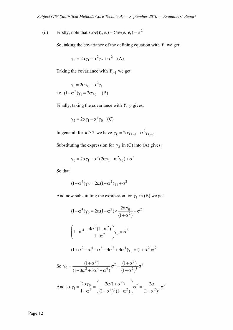
Subject CT6 (Statistical Methods Core Technical) — September 2010 — Examiners’ Report
Page 12
(ii) Firstly, note that 2( , ) ( , )t t t tCov Y e Cov e e= = σ So, taking the covariance of the defining equation with tY we get: 2 2
0 1 22γ = αγ −α γ + σ (A) Taking the covariance with 1tY − we get 2
1 0 12γ = αγ −α γ
i.e. 21 0(1 ) 2+α γ = αγ (B)
Finally, taking the covariance with 2tY − gives: 2
2 1 02γ = αγ −α γ (C) In general, for 2k ≥ we have 2
1 22k k k− −γ = αγ −α γ Substituting the expression for 2γ in (C) into (A) gives: 2 2 2
0 1 1 02 (2 )γ = αγ −α αγ −α γ +σ So that 4 2 2
0 1(1 ) 2 (1 )−α γ = α −α γ +σ And now substituting the expression for 1γ in (B) we get
4 2 200 2
2(1 ) 2 (1 )(1 )αγ
−α γ = α −α × +σ+α
2 2
4 202
4 (1 )11
⎛ ⎞α −α−α − γ = σ⎜ ⎟⎜ ⎟+ α⎝ ⎠
2 4 6 2 4 2 2
0(1 4 4 ) (1 )+α −α −α − α + α γ = +α σ
So 2 2
2 20 2 4 6 2 3
(1 ) (1 )(1 3 3 ) (1 )
+α +αγ = σ = σ
− α + α −α −α
And so 2
2 201 2 2 3 2 2 3
2 2 (1 ) 21 (1 ) (1 ) (1 )
⎛ ⎞αγ α +α αγ = = σ = σ⎜ ⎟⎜ ⎟+ α −α +α −α⎝ ⎠
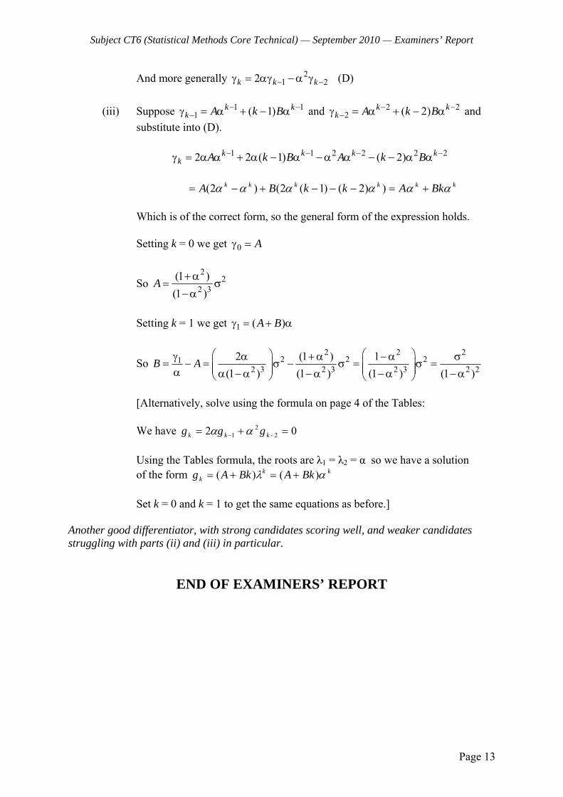
Subject CT6 (Statistical Methods Core Technical) — September 2010 — Examiners’ Report
Page 13
And more generally 21 22k k k− −γ = αγ −α γ (D)
(iii) Suppose 1 1
1 ( 1)k kk A k B− −−γ = α + − α and 2 2
2 ( 2)k kk A k B− −−γ = α + − α and
substitute into (D). 1 1 2 2 2 22 2 ( 1) ( 2)k k k k
k A k B A k B− − − −γ = α α + α − α −α α − − α α kkkkkk BkAkkBA αααααα +=−−−+−= ))2()1(2()2( Which is of the correct form, so the general form of the expression holds. Setting k = 0 we get 0 Aγ =
So 2
22 3
(1 )(1 )
A +α= σ
−α
Setting k = 1 we get 1 ( )A Bγ = + α
So 2 2 2
2 2 212 3 2 3 2 3 2 2
2 (1 ) 1(1 ) (1 ) (1 ) (1 )
B A⎛ ⎞⎛ ⎞γ α + α −α σ
= − = σ − σ = σ =⎜ ⎟⎜ ⎟⎜ ⎟ ⎜ ⎟α α −α −α −α −α⎝ ⎠ ⎝ ⎠
[Alternatively, solve using the formula on page 4 of the Tables: We have 02 2
21 =+= −− kkk ggg αα
Using the Tables formula, the roots are λ1 = λ2 = α so we have a solution of the form kk
k BkABkAg αλ )()( +=+= Set k = 0 and k = 1 to get the same equations as before.] Another good differentiator, with strong candidates scoring well, and weaker candidates struggling with parts (ii) and (iii) in particular.
END OF EXAMINERS’ REPORT


![PC03 – MS Word 2010 · A Microsoft Access 2010 Microsoft InfoPath Designer 2010 [0 2010 Microsoft OneNote 2010 Outlook (i] Pbcrosoftpowerpont2010 Microsoft Publisher 2010 word Ejecutar](https://img.pdfslide.us/doc/110x75/5f6cc4583f95123b051799c8/pc03-a-ms-word-2010-a-microsoft-access-2010-microsoft-infopath-designer-2010-0.jpg)