Embed Size (px)
Citation preview

DOT/FAA/CT-93177 DOT-VNTSC-FAA-93-7
FAA Technical Center Atlantic City International Airport, N.J. 08405
.. ·· ··-~~-
December 1993
Final Report
0 . U.S. Department of Transportation Federal Aviation Administration

rlroek, David J/ Analysis concerning
the inspection threshold for multi-site damage
der the sponsorship of the the interest of information ment assumes no liability for
ts not endorse products or rers' names appear herein :sential to the objective of this

REPORT DOCUMENTATION PAGE Form Ap!?roved OMB No. 704-0188
Public reporting burden for this collection of information is estimated to average 1 hour per response, includirl9 the time for reviewing instructions( searchi~ existi~ data sources, gathering and maintaining the data needed, and CC!q)letil)9 and reviewil)9 the co lection o informa ion. Send cannents regardi!'19 this burden estimate or anv. other as~t of this collection of information, including s~.~ggestions for reducing th1s burden, to Washin~ton Heai;lquarters ~~5X~~!~11,Di~t~~ef8~!o~tion Operat!~R~~ .. ~e~rts, 1215R~~!:~~onp~:y,i~t ":R~~!~{) 1 ~tte"'!;~~a~~~"H~~{)5X~ 1. AGENCY USE ONLY (Leave blank) 2. REPORT DATE 3. REPORT TYPE AND DATES COVERED
December 1993 Final Report April 1991 - June 1991
4. TITLE AND SUBTITLE 5. FUNDING NUMBERS Analysis Concerning the Inspection Threshold for Multi-Site Damage
FA3H3/A3128 6. AUTHOR(S) DTRS57-91-P-80859 David Broek
7. PERFORMING ORGANIZATION NAME(S) AND ADDRESS(ES) 8. PERFORMING ORGANIZATICJI FractureREsearch, Inc. * REPORT NUMBER 9049 Cupstone Drive DOT-VNTSC-FAA-93-7 Galena, OH 43021
9. SPONSORING/MONITORING AGENCY NAME(S) AND ADDRESS(ES) 10. SPONSORING/MONITOIIIIC u.s. Department of Transportation AGENCY REPORT MUMIII Federal Aviation Administration Technical Center
DOT/FAA/CT-93/77 Engineering, Research, and Development Service Atlantic City International Airport, NJ 08405
11. SUPPLEMENTARY NOTES u.s. Department of Transportation * under contract to: Research and Special Programs Administration
Volpe National Transportation Systems Center Cambridge, MA 02142-1093
12a. DISTRIBUTION/AVAILABILITY STATEMENT 12b. DISTRIBUTION caDI
This document is available to the public through the National Technical Information Service, Springfield, VA 22161
13. ABSTRACT (Maximum 200 words)
Periodic inspections, at a prescribed interval, for Multi-Site Damage (MSD) in longitudinal fuselage lap-joints start when the aircraft has accumulated a certain number of flights, the inspection threshold. The work reported here was an attempt to obtain justification for the threshold. It is based upon an analysis of fatigue data for lap-joints (riveted as well as riveted plus bonded) of a configuration closely resembling those in several types of aircraft. Depending upon the definition of threshold, the results show that it will be around 30,000 flights. Graphs are supplied upon the basis of which airworthiness authorities can determine a threshold in accordance with their preferred definition, and for different service conditions.
14. SUBJECT TERMS 15. NUMBER OF PAGES
(MSD), fuselage, lap-joints, threshold 50
Multi-Site Damage 16. PRICE CODE
17. SECURITY CLASSIFICATION 18. SECURITY CLASSIFICATION 19. SECURITY CLASSIFICATION 20. LIMITATION OF ABSTRACT OF REPORT OF THIS PAGE
Unclassified Unclassified
NSN 7540·01-280·5500
OF ABSTRACT Unclassified
Standard Form 298 (Rev. ~.-1!9; Prescribed by ANSI Std. 239-~8 298·102

PREFACE
Periodic inspections, at a prescribed interval, for Multi-Site Damage (MSD) in longitudinal fuselage lap-joints start when the aircraft has accumulated a certain number of flights, the inspection threshold. The work reported here was an attempt to obtain justification for the threshold. It is based upon an analysis of fatigue data for lap-joints (riveted as well as riveted plus bonded) of a configuration closely resembling those in several types of aircraft. Depending upon the definition of threshold, the results show that it will be around 30,000 flights. Graphs are supplied upon the basis of which airworthiness authorities can determine a threshold in accordance with their preferred definition, and for different service conditions.
This report was prepared for the Volpe National Transportation Systems Center in support of the Federal Aviation Administration Technical Center under contract DTRS57-91-P-80859.
iii

METRIC/ENGLISH CONVERSION FACTORS
ENGLISH TO METRIC
LENGTH (APPROXIMATE)
inch (in) • 2.5 centimeters (em)
1 foot (ft) = 30 centimeters (em) 1 yard (yd) = 0.9 meter (m)
1 mile (mi) = 1.6 kilometers (km)
AREA (APPROXIMATE)
square inch (sq in, in2 • 6.5 square centimeters cem2> 1 square foot (sq ft, ft2 = 0.09 square meter (~)
1 square yard (sq yd, ~) = 0.8 square meter cm2> 1 square mile (sq mi, mi2) = 2.6 square kilometers (~) 1 acre = 0.4 hectares (he) = 4,000 square meters (m2>
MASS • WEIGHT (APPROXIMATE)
1 ounce (oz) = 28 grams (gr) 1 pound (lb) = .45 kilogram (kg)
1 short ton= 2,000 pounds (lb) = 0.9 tonne (t)
VOLUME (APPROXIMATE)
teaspoon (tsp) = 5 mHlHiters (ml)
1 tablespoon (tbsp) = 15 milliliters (ml)
1 fluid ounce (fl oz) = 30 milliliters (ml)
1 cup (c) = 0.24 Liter (1)
1 pint (pt) • 0.47 Liter (1)
1 quart (qt) = 0.96 liter (1)
gallon (gal) = 3.8 liters (1)
1 cubic foot (cu ft, ft3) = 0.03 cubic meter cm3> cubic yard (cu yd, vd3> = 0.76 cubic meter cm3)
TEMPERATURE (EXACT)
[(x-32)(5/9)) °F = y 0c
METRIC TO ENGLISH
LENGTH (APPROXIMATE)
1 millimeter (mm) = 0.04 inch (in)
1 centimeter (em) = 0.4 inch (in) 1 meter (m) = 3.3 feet (ft)
1 meter (m) = 1.1 yards (yd)
kilometer (km) • 0.6 mile (mi)
AREA (APPROXIMATE)
1 square centimeter (em2) • 0.16 square inch (sq in, tn2)
1 square meter cm2> = 1.2 square yeards (sq yd, ~) 1 square kilometer (~) = 0.4 square mile (sq mi, mi2)
1 hectare (he) = 10,000 square meters (m2) • 2.5 acres
MASS · WEIGHT (APPROXIMATE)
1 gram (gr) = 0.036 ounce (oz) kHogram (kg) = 2.2 pounds (lb)
1 tonne (t) = 1,000 kilograms (kg) • 1.1 short tons
VOLUME (APPROXIMATE)
1 milliliters (ml) • 0.03 fluid ounce (fl oz)
1 liter (1) = 2.1 pints (pt)
1 liter· (1) • 1.06 quarts (qt)
1 liter (1) = 0.26 gallon (gal)
1 cubic meter (m3) = 36 cubic feet (cu ft, ft3)
1 cubic meter (~) = 1.3 cubic yards (cu yd, vd3>
TEMPERATURE (EXACT)
[(9/5) y + 32) °C = X °F
QUICK INCH-CENTIMETER LENGTH CONVERSION
INCHES 0 2 3 4 5 6 7 8 9 10
CENTIMETERS 0 2 3 4 5 6 7 8 9 10 11 12 13 14 15 16 17 18 19
QUICK FAHRENHEIT-CELSIUS TEMPERATURE CONVERSION
OF ·40° -22° -40 14° 32° 50° 680 860 104° 122° 140° 158° 176° 194° 212° I I
-2b0 I bo I I 3b0 4b0 5b0 Jo I Jo
·I I oc -40° -30° -10° 10° 20° 70° 90° 100° 1
For more exact and or other conversion factors, see NBS Miscellaneous Publication 286, Units oJ Weighfs and Measures. Price S2.50. SO Catalog No. C13 10286.
iv

TABLE OF CONTENTS
Section
1.
2.
3.
4.
5.
6.
INTRODUCTION AND SCOPE • •
AVAILABLE DATA •
2.1 2.2
Description of Database • • • • • • Scatter and Distribution Function •
DISTRIBUTION OF INITIATION LIFE IN PRACTICE
. • 1
• • 2
• • • 2 • • • 3
• • 5
3.1 Estimate of Applicable S-N CUrve •••••• 5 3.2 Calculation of Initiation and Scatter •••••••• 7
CONSIDERATIONS FOR THRESHOLD . . . . . . . . . . . . . . 10
4.1 Definition of Threshold . . . . . . . . 10 4.2 Resulting Flight Numbers Till Threshold . . . . 11 4.3 The Crack Growth Approach . . . . . . . 11
CONCLUSION . . . . . . . . . . . . . . . . . 13
REFERENCES . . . . . . . . . . . . . . . . . . . 14
v

Figure
1o
2o
LIST OF FIGURES
TESTS BY HARTMAN . . . . . . . . . . . . . . . . ALL DATA FOR FAILURES IN ADHESIVE; NOT AT HOLES - ALL CONDITIONS (HARTMAN DATA FOR RIVETED PLUS BONDED LAP-JOINTS) o o
3o ALL DATA FOR FAILURES AT HOLES (HARTMAN DATA FOR RIVETED AND BONDED LAP-JOINTS;
4o
5o
6o
7o
8o
9o
10o
11.
12o
13o
14o
HARTMAN DATA) o o o o o o o o o o o o o o
HARTMAN DATA FOR LAP-JOINTS RIVETED PLUS BONDED AND RIVETED ONLY (CONSOLIDATION OF ALL HARTMAN DATA) o o o o o o o o o o
TESTS ON SPECIMEN WITH SIMULATED TEAR STRAPS [ 6, 7 ] o o o o o o o o o o o o
COMPARISON OF MEAN S-N CURVES o o o o o o
HOLE-FAILURES AT HIGH AND LOW FREQUENCY -ADHESIVE AND NON-AGED (HARTMAN DATA FOR
. . . .
RIVETED PLUS BONDED LAP-JOINTS) o o o o o o o o o
DATA FOR ALL HOLE FAILURES: HIGH AND LOW FREQUENCY - ADHESIVE AGED AND NON-AGED (HARTMAN DATA FOR RIVETED PLUS BONDED) o o o
GROWTH OF LARGEST CRACK IN 10 RUNS
MEASURED CRACK GROWTH CURVES [6,7]
S-N CURVES USED IN ANALYSIS
. . . . . . .
. . . . . . . 0 0
OPTIMISTIC CASE WHERE ALOHA BELONGS TO LOWER 15 PERCENTILE o o o o o o o
CASE IN WHICH ALOHA BELONGS TO LOWER 25 PERCENTILE o o o o o o o o o o o o o o o
CONSERVATIVE CASE WHERE ALOHA IS AVERAGE
15o THREE CASES FOR DIFFERENTIAL PRESSURE OF
16o
. 8 ps.1 • • • • • • • • • • • • • • • • • •
FINAL CRACK SIZES AT ALL LOCATIONS - SAME CASE AS IN FOLLOWING - SOLID LINE: LEFT CRACK; DASH-DOT; RIGHT CRACK o o o o o o
vi
. . . .
15
16
17
18
19
20
21
22
23
24
25
26
27
28
29
30

Figure
17.
18.
19.
20.
21.
22.
23.
LIST OP PIGURES (continued)
CUMULATIVE PROBABILITY OF DETECTION PER LOCATION - SOLID LINE: EDDY CURRENT; DASH-DOT LINE: VISUAL INSPECTION INTERVAL 3000 CYCLES; TYPICAL CASE • • • • • • • • •
MEASURED CRACK SIZES AT FAILURE [6,7] •••
SIZES OF DETECTED MSD IN AIRCRAFT [6,7] ••
SIZE DISTRIBUTION WHEN LARGEST CRACK IS 0.1 INCH • • • • • • • • • • • • • • •
NUMBER OF CRACKS AND SIZE OF LARGEST CRACK - EXAMPLE OF STATICALLY ARBITRARY CASE
SIZE DISTRIBUTION WHEN LARGEST CRACK IS
. . 0.1 INCH . . . . • . . . • . • . . . . . . . . . SUMMARY OF RESULTS - LIFE UNTIL 1 PERCENT CRACKED • • • • • • • • • • • • • • • • •
24. SUMMARY OF RESULTS - LIFE UNTIL 2 PERCENT
25.
26.
27.
28.
CRACKED • • • • • • • • • . . . . . SUMMARY OF RESULTS - LIFE UNTIL 5 PERCENT CRACKED • • • • • • • • • • • • •
SUMMARY OF RESULTS - CASE WHERE ALOHA BELONGS TO LOWER 25 PERCENTILE • • •
CRACK GROWTH; RUN ID: 17685 AT DIFFERENT MAXIMUM PRESSURES STARTING AT 0.005 INCH . . . . LIFE UNTIL 0.12 INCH CRACK AS A FUNCTION OF ASSUMED EQUIVALENT INITIAL FLAW (EIF) SIZE
vii/viii
31
32
33
34
35
36
37
38
39
40
41
42

1. INTRODUCTION AND SCOPE
The cumulative probability of detection of Multi-Site Damage (MSD) in fuselage lap-joints of aging aircraft was assessed in a previous study [1]. It showed that inspection intervals on the order of 3000 to 4000 flights provide cumulative probabilities of detection on the order of 0.98 (98 percent detected) or better if inspections are performed by eddy current. Although quite a few assumptions were necessary, a sensitivety analysis showed the effect of the assumptions to be small.
It is unlikely for MSD to occur very early in life, because disbonding of the adhesive will take some time. Therefore, and because the probability of detection is virtually zero in the early stages of MSD, it is un-economical to adhere to the prescribed inspection interval from time zero. Hence an inspection threshold was instituted by stipulating that inspections for MSD need not start until after the accumulation of a certain number of flights. The present study was undertaken to provide a justification for this threshold.
As the alotted time for this work was very limited, only readily available results of fatigue tests on lap-joints were analyzed. The test data were used primarily to obtain the scatter (i.e. distribution function) for the start of cracking: the scatter determines when the earliest detectable MSD may occur. The only true service experience comes from the Aloha incident. The time to failure for the latter case was used as the anchor point for the estimate of the fatigue-life curves (S-N curves) for service conditions. As this approach needed only a few reasonable assumptions, it is considered to provide a realistic assessment of the threshold.
Another procedure to determine inspection thresholds is based upon crack growth analysis. It is then assumed that a certain crack is already present in the new structure, and the time it takes for this initial crack to grow to a "detectable" size, is used for the inspection threshold, either directly or with a safety factor. This procedure has found some acceptance by the industry and by FAA certification offices. The initial "crack" is not a real crack but rather an Equivalent Initial Flaw (EIF), where the qualifier "equivalent" indicates that if the EIF is used in analysis, it will lead to acceptable results. Unfortunately, the results depend strongly upon the assumed size of the EIF, while the commonly used value of 0.05 inch cannot very well be justified. Nevertheless, this approach was used in the present work as well to obtain a comparison with the analysis based upon fatigue life. The results are of the same order of magnitude as those based upon life analysis.
1

2. AVAILABLE DATA
2.1 DBSCRIPTIOH OP DATA BASB
Readily available fatigue test data for joints were those in References 2 through 8. A diligent search of older reports (19S0-196S) by NACA (NASA), RAE, NLR, FFA, ARL, and so on, is likely to provide a wealth of additional data, but time constraints did not permit such a search and associated data analysis. Of the sources readily available some were for conditions and configurations not immediately relevant to the problem at hand, but the large data base generated by Hartman [2] is very appropriate, as are a few data generated recently [6,7].
It should be noted that in all of the following the stresses are the nominal stresses away from the joint: they represent the hoop stress in a fuselage. This simulated hoop stress is not necessarily equal to that due to presurization, as will be explained later. Furthermore, all data are for a stress ratio, R, of o.os to 0.1, while fuselage loading is essentially at R = o. As a consequence, the assumption had to made that the results are applicable to the slightly different fuselage loading, but this of minor importance because the effect of the associated difference in mean stress is small.
Hartman's data [ 2] are especially useful, because they were obtained from tests on adhesively bonded and riveted lap-joints of a configuration (Figure 1) almost identical to the one used in the fuselage of several types of aircraft. Hartman performed well over 400 tests. The lap-joints specimens were bonded with a cold-curing adhesive, and contained 3 rows of countersunk fasteners. Hartman investigated the effect of many parameters, the most important of which are: (1) Two adhesives, namely AW106 (CIBA) and EC226 (3M); ( 2) two types of surface treatment, namely chromic acid and sulphuric acid anodizing; (3) Three testing temperatures, namely -sse (stratosphere), 20C and soc (aircraft taking of after exposure to summer sun at airport); (4) in one series of tests the adhesive was intentionally maltreated by exposure to 100% RH at70C for 4 weeks; (S) three loading frequencies, namely 6, 240 and 3000 cpm; (6) several different stress levels.
Part of the specimens failed at the adhesive fillet or elsewhere away from the fastener holes. These data, regardless of test parameter, are shown in Figure 2. As MSD occurs at the fastener holes, these data were excluded from the following analysis. Well over 200 of Hartman's specimens failed at the fastener holes. They are shown in Figure 3, again regardless of test parameters. Hartman did a limited number of tests on specimens that were riveted only (as opposed to riveted and bonded). The data of these tests are shown in Figure 4. Also shown in Figure 4 are the data points obtained at low frequency loading (which is the most relevant for longitudinal fuselage joints) for riveted plus bonded joints which failed at the holes.
2

The data obtained by Mayville [6,7] deserve attention. Instead of the basic lap-joints as used by Hartman, Mayville employed the specimen shown in Figure 5. Two short stiffeners were attached to the edges of the specimens to simulate the crack arrester straps (tear straps) found in some types of aircraft experiencing MSD. A finite element analysis [9] had shown the stresses at the lap-slpice to be higher midway between the straps. Strain gage measurements showed that the stress distribution in the test panels with the simulated tear straps was nearly identical to the one obtained from the finite element analysis. This is shown convincingly in Figure 5.
The test data from these panels, although limited, may be more representative of the situation in some aircraft, but it should be noted that the joints were riveted only (not riveted and bonded), and that they were obtained at high frequency loading. A total of 10 data points was available; in 6 of the specimens the fasteners had driven heads of nominally 0. 24 inch diameter, while in the others this dimension was 0.25 inch. The data points for all are shown in Figure 6. Those for the small driven heads fall below Hartman's scatter band; the others fall inside the scatterband. This indicates that the non-uniform stress distribution in the specimens (Figure 5) has but little effect. Figure 6 shows average lives for various conditions investigated by Hartman. In addition a line is shown labeled "Grover" [ 8] • Although Grover [ 8] does not identify his sources, nor the details of the specimen used, at least the curve falls within the scatterband of Hartman's data in the regime of stresses relevant to the problem of longitudinal fuselage lap-joints.
2.2 SCATTER AND DISTRIBUTION FUNCTION
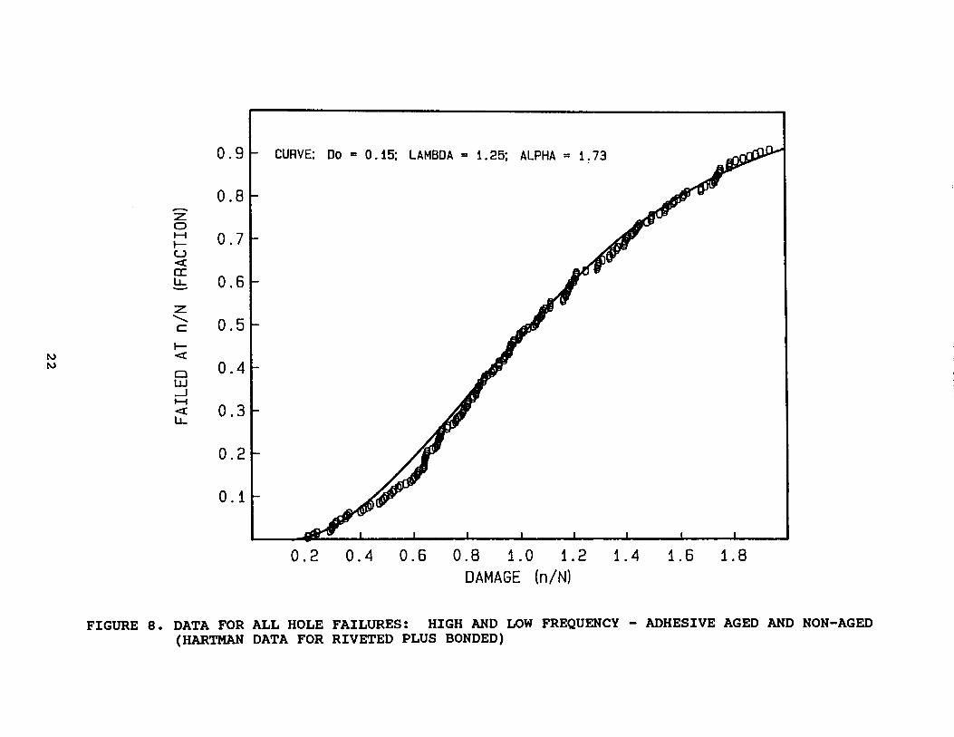
As is normal in the case of fatigue (especially at lower stresses), the scatter in Figures 3 and 4 is large. Admittedly, this scatter is somewhat exaggerated because all data for all conditions are plotted in the same graph; the justification for this will follow. Despite the large number of tests, the number of data points per stress level and per case is still very small and would yield distribution functions containing much uncertainty. This problem was solved by the use of the fatigue damage at failure according to Miner's rule, njN, where n is the actual number of cycles to failure, and N the average life at the same stress level. The advantage of this is that data for all stress levels are consolidated. To obtain the distribution function, only those data were considered that pertain to failure at the rivet holes (Figures 3,4,6), as these are the most relevant to MSD.
This leaves about 200 data points for which the distributions are shown in Figure 7. Scatter for the individual cases is very similar to the total scatter in Figure 8 indicated by the fact that they all go from njN = 0. 2 to 2 (plus) • Besides, the distribution functions are the same, as all data follow the same curve reasonably well. In the case of actual aircraft almost all conditions investigated by Hartman will appear part of the time.
3

Therefore all data were considered to belong to one population covering all service conditions for aircraft. This leads to the distribution function shown in Figure a. Not only is this general distribution function the same as the one for the individual cases in Figure 7, it turns out that the data fit the Weibul distribution very well.
Miner's rule predicts crack inititation if Sum n/N = 1. The data show that due the scatter, failure occurs at values between 0.15 and 2. The Weibul parameters in Figure a were more or less confirmed by other data [3,4,5]. The distribution function is:
Pf = 1 - exp(- (n/N- Do)/(A- Do)A X)
where Pf is the fraction (percentage) failed, or probability of failure, while Do, A, and X are the shape parameters the values of which are shown in Figures 7 and a. The average (Pf = 0.5) is indeed at n/N = 1.
4
3. DISTRIBUTION OF INITIATION LIFE IN PRACTICE
3.1 ESTIMATE OF APPLICABLE S-N CURVE
Although the above provides the distribution of n/N, the actual average life, N, under aircraft service conditions is not known. However, one important actual service data-point is available from the Aloha incident: the failure occured at 89600 flights. Accounting for the fact that the average time for crack growth to failure is 25,000 flights the initiation time is estimated at 64,000 flights.
The average of 25,000 flight cycles for crack propagation follows from previous work [10] in which crack growth was calculated for a variety of statistical parameters (assigned by a Monte-Carlo technique) and for a variety of circumstances. An example of these computations is shown in Figure 9. The number is confirmed by data obtained by Mayville [6,7] shown in Figure 10. Although the crack growth curves in Figure 10 start at different cycle numbers, they are well-nigh parallel. The total growth from initiation to failure covers about 20,000 to 25,000 cycles, if initiation is considered as the appearance of a crack of about o. 02 inch size. From a practical point of view this is a good definition, because at 0.02 inch the crack will just emerge from under the fastener head and become inspectable.
The remaining question is then where the Aloha case falls in the scatter band, i.e. whether the case is an extreme. One might argue that it is, because Aloha operates in adverse conditions (low altitude flights over sea). But MSD was detected in many other aircraft as well, indicating that Aloha was not an extreme. Three cases were considered, namely:
1. Aloha is average (or 50 percentile; conservative). 2 Aloha belongs to the lower 25 percentile • 3. Aloha belongs to lower 15 percentile (optimistic; it is
an extreme) •
For each of these percentiles the value of n/N can be read from Figure 8, from which the average life N can be found. Making the reasonable assumption that all S-N curves have the same slope, the life-to-initiation curves for the above 3 conditions, and for the stress levels encountered in service can be determined to be as shown in Figure 11, and as explained below.
For the relevant stress ranges in the regime of 10 to 20 ksi the sN curve can be represented by a straight line on semi-logarithmic scales, and hence by the equation:
S =A - q ln N
5

which can be inverted to:
N = exp ((A - S) Jq)
where N is the life to crack initiation, S the stress range, and A and q are parameters. That all lines should be parallel (same slope) in the region of interest can be ascertained from Figures 3, 4, and 6; this results in a fixed value for q of 2.74. (Although the data in the previous figures were plotted, in accordance with engineering practice, on 10-log scale, the natural logarithm was used in the equations.) Hence, the difference in the lines shown in Figure 11 is characterized by different values of A.
As flights are of different length the cruising altitude (and hence the differential pressure) varies from flight to flight. This means that the loading is not of constant amplitude. Since the s-N curves were to be "anchored" on the Aloha case, the Aloha experience service experience is detailed below:
Altitude Del ta-p % of flights Pressure relative to highest (ft) (psi)
>18000 7.5 23 1.00 16000 6.7 5 0.89
<14000 6.1 72 0.81
According to the finite element analysis [9] the membrane stress at mid-bay is 14.9 ksi, but this number is for a skin thickness of 0.04 inch and a differential pressure of 8.5 psi. In the actual aircraft the maximum pressure was 7.5 psi (above table), bringing the maximum operating stress to 14.9 * 7.5/8.5 = 13.15 ksi. Due to the lower skin thickness another 10 percent must be added, which provides a maximum stress of 14.5 ksi.
If the Aloha case was the average (50 %) crack inititiation, as defined above, occurred at nJN = 1, at 64,000 cycles as explained. The table shows that the highest stress of 14.5 ksi occurred in 23 percent of the flights, i.e. in 0.23 * 64,000 = 14,720 flights.
The membrane stress in the other flights at differential pressures of 6.7 and 6.1 psi are obtained as 14.5*6.7/7.5 = 13 ksi, and 14.5 * 6.1/7.5 = 11.8 ksi, respectively. The associated cycle numbers are o.os * 64,000 = 3,200, and 0.72 * 64,000 = 46,000, respectively.
With this information a system of 4 equations with 4 unknowns can be solved to obtain A. The result is A = 43, so that the equation for the life becomes:
N = exp((43 - S)/2.74)
6

The membrane stress in the other flights at differential pressures of 6.7 and 6.1 psi are obtained as 14.5*6.7/7.5 = 13 ksi, and 14.5 * 6.1/7.5 = 11.8 ksi, respectively. The associated cycle numbers are 0.05 * 64,000 = 3,200, and 0.72 * 64,000 = 46,000, respectively.
With this information a system of 4 equations with 4 unknowns can be solved to obtain A. The result is A = 43, so that the equation for the life becomes:
N = exp((43 - S)/2.74)
Inverting this procedure permits calculation of sum n/N for this case as follows:
s (ksi) n N (for A = 43) n/N
14.5 14,720 32,900 0.447 13.0 3,200 56,900 0.056 11.8 46,000 88,200 0.522
Sum n/N 1.025
Hence, if Aloha is an average case, the S-N curve with A = 43, shown in Figure 11, is the applicable curve for the average life to initiation. For the other cases defined above a similar procedure leads to the average S-N curve. However, it can be seen immediately what the results will be, because all calculations are based upon proportionality. Figure 6 shows that for a probability of initiation of 25 percent the value of njN = o. 70, while for a probability of 15 percent it is 0.52. Thus it can be deduced immediately that the associated lives for all stresses are higher by a factor of 1/0.70 = 1.43, and 1/0.52 = 1.92 respectively, leading to values for A of 44 and 44.8 respectively; these are represented by the other lines in Figure 11.
Although superfluous, it should be pointed out that for the following computations the lines in Figure 11 should be interpreted as averages. For example, if the line for A = 43 is the average, the Aloha case will be average (as signified by the Aloha case falling on this line); but if the line for A= 44 is the average, the Aloha case falls left of the line, as shown in Figure 11. The curves in Figure 11 pertain to the average life N. To this the scatter (distribution function) of Figure 8 was applied.
3.2. CALCULATION OF INITIATION LIFE AND SCATTER
The S-N curve(s) and distribution function now being known, the life to initiation can be calculated. To this end a small computer program was developed. The program employs the membrane stresses
7

across a bay as calculated by the finite element analysis [9] for a pressure differential of 8.5 psi (Figure 5), as shown below:
l.l. l. ksi (at frame and straps) at l.O% of holes 1.2.6 ksi at 20% of holes 1.3.8 ksi at 20% of holes 1.4.5 ksi at 20% of holes 1.4.8 ksi at 20% of holes 1.4.9 ksi (midbay) at l.O% of holes
The nominal membrane stress was used in the analysis, because all data previously discussed are in terms of this nominal stress. The nominal stress for any pressure differential the can be obtained by multiplying the above stresses by p/8.5.
Many airlines service longer routes than Aloha, so that their maximum pressure (altitude) will be higher. It seems reasonable however, lacking data from other airlines, to assume that the last two columns in the Aloha usage table provide an appropriate estimate of "general" usage relative to maximum pressure differential. Therefore, the calculations were based upon a usage spectrum in accordance with the one shown for Aloha, relative to a maximum operating pressure of l., and Miner's rule for the accumulation of damage at the three stress ranges (differential pressures). The maximum operating pressure differential is then the only variable, because the other pressures are given relative to the maximum. It permits computation of the membrane stresses at the holes according to the conversion rule discussed, and subsequently, assessment of the damage, Sum njN, according to the generalized usage spectrum.
Apart from being directly dependent upon fuselage pressurization, the membrane stress depends upon aerodynamic pressure. The aerodynamic pressure varies from point-to-point due to the fuselage shape, but should be assessed at about 0.5 psi on average (1.2] • This will increase the pressure differential locally, and hence, the membrane stresses will be higher than those following from fuselage pressurization. This may explain why MSD appears to be more prevalent at joints in the fuselage ~rown just behind the flight deck. Another area where this effect is significant is the vicinity of the wing-fuselage connection.
If the pressure differential by fuselage pressurization is for example 8 psi, the actual local pressure differential would be on the order of 8.5 psi, and possibly higher close to the wingfuselage connection. The above was invoked in the small computer program already mentioned.
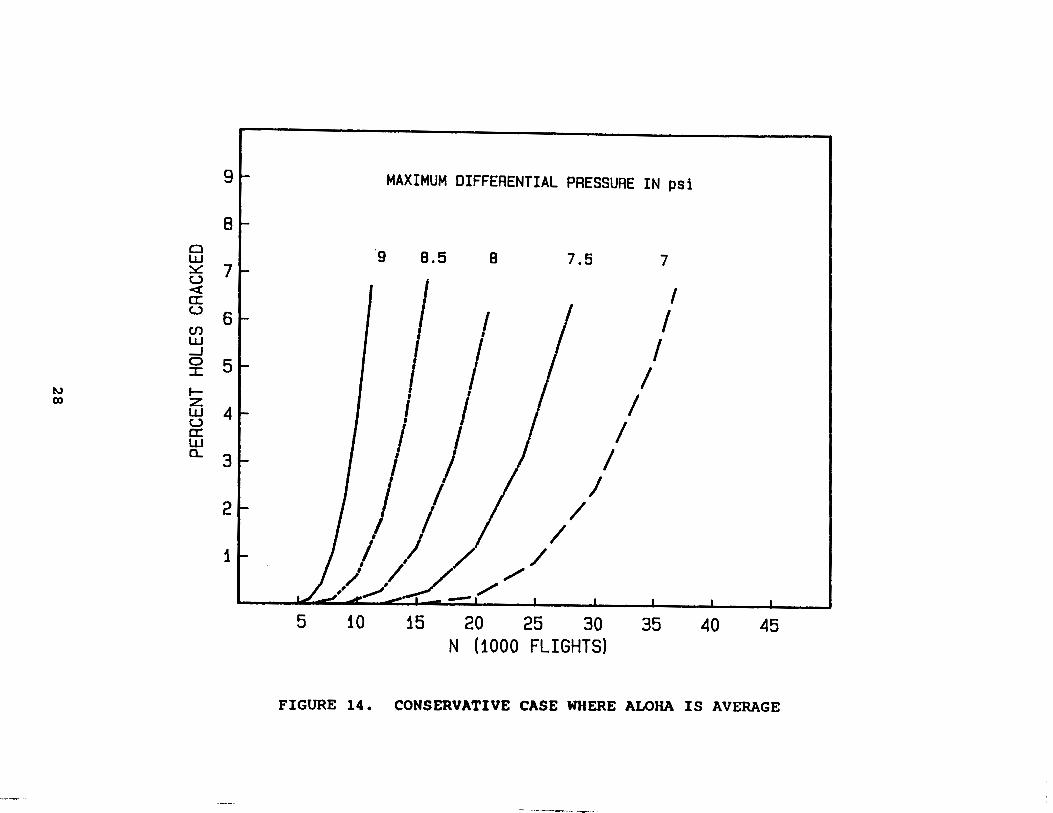
Accounting for all the effects discussed above calculations were made of the per cent failed (holes cracked). The computations were cintinued until l.O percent of the holes were cracked, for the cases discussed and for different pressures. The results of the computations are shown in Figures 1.2 through 1.4 for various pressure differentials (as adjusted for usage spectrum and local
8

aerodynamic pressure), and for cases where the Aloha case is the lower 15, 25 and 50 percentile. For a particular maximum pressure differential of 8 psi (accounting for an aerodynamic differential of 0.5 psi), the results are shown in Figure 15. Similar cross plots can be made for other pressures by using the data in Figures 12 through 14. The results are trivial in a way, because they merely restate the lower end of the distribution function for a particular set of circumstances.
9

4. COHSXDERATXOHS FOR THRESHOLD
4.1. DEPXHXTXOH OP THRESHOLD
A more specific definition of threshold is now needed. In essence the threshold is the time at which inspections must be started. There is no use for inspections as long as the cracks cannot be found, i.e. if they are so small that the probability of detection is virtually zero. From execution of the computer program for crack detection [10], it is known that the largest crack is on the orderr of 0.06 inch when 2 percent of the holes is cracked and 0.12 inch when 5 percent is cracked; all other cracks are smaller. In view of that the probability of detection is virtually zero. Although the results can vary considerably in different computer runs (the code simulates statistical variability by means of a Monte-Carlo technique [ 10]) , the above numbers are considered reasonably conservative.
Since the following arguments will be based upon the results of a computer program developed previously [10], it seems appropriate to demonstrate that the computations provide results in concert with actual observations of MSD. Figure 16 shows an example of computed crack sizes at 100 holes at the time of failure, while Figure 17 shows the computed cumulative probability of detection of these cracks. Figure 16 should be compared with Figures 18 and 19. The latter two figures show the MSD crack sizes as observed by Mayville [6,7] in test panels (Figure 18), and as detected in an aircraft (Figure 19). Apparently, the computations produce a "true-to-life" picture.
The computer program was therefore used to produce the MSD crack sizes for the situation where the largest crack is 0.06 inch, and 0.1 inch respectively. Only two examples will be provided. Figure 20 shows a case where the fraction of holes cracked is 0.09 (9 percent cracked), while Figure 21 shows the growth curve of the largest crack as well as the number of cracks as a function of the number of (flight) cycles. As already mentioned, the results vary considerably from run to run. A rather extreme case in which already 39 percent of the holes are cracked - the largest crack still being 0.1 inch - is shown in Figure 22.
More important than Figures 20 and 22 would be the figures showing the cumulative probability of detection (in the manner shown in Figure 17). However, these figures would exhibit the "scales" only, because the cumulative probability of detection was virtually zero in all cases and, therefore, would not show in the graphs. These calculations were done for an inspection interval of 3000 flights. Had the interval been selected larger than this, the probability of detection would have been less (if less than zero were possible). Naturally, shorter intervals would show higher cumulative probability of detection, but that is of academic interest only, because the interval is not less than 3000 flights.
10

4.2 RESULTING FLIGHT NUMBERS TILL THRESHOLD
The results indicate that the definition of threshold may well be the time at which 5 percent of the holes are cracked, because the cumulative probabilty of detection would still be virtually zero. However, it is not the charter of the author of this report to suggest what the threshold should be. This report merely provides information upon which the authorities can base a decision.
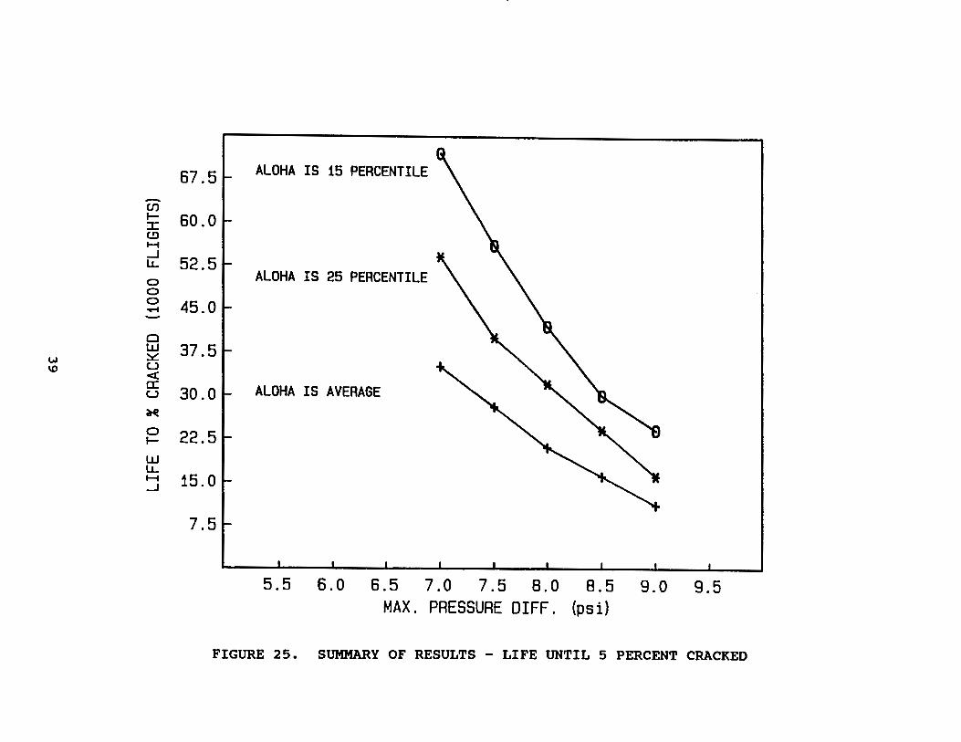
For this reason thresholds defined by 1, 2 and 5 percent cracked were considered. The number of flights for reaching these can be obtained from the basic results provided in Figures 12 through 14. To facilitate interpretation additional cross plots were made for the percentages mentioned above. These are shown in Figures 23 through 26.
The following may serve as an example of how these figures should be interpreted. If one is willing to assume that the Aloha case belongs to the lower 25 percentile, that the maximum operating pressure is 8 psi, and that 5 percent cracked is a good definition of threshold, the resulting threshold would be 34,000 flights (Figures 25 and 26). With very conservative assumptions (Aloha is average, 2 percent cracked, maximum operating pressure of 9 psi), the threshold would be 10,000 flights (Figure 24).
4.3 THB CRACK GROWTH APPROACH
Inspection thresholds are sometimes determined by means of crack growth analysis. In that case a certain initial crack, denoted as the Equivalent Initial Flaw (EIF), is assumed present in the new structure. The time (number of cycles) it takes for this EIF to grow to a detectable size is used as the basis for the inspection threshold. The EIF is often taken as 0.05 inch; this size is based upon a somewhat arbitrary EIF determined by the USAF, as explained below.
The USAF [11,12] examined the cracks that developed during a fullscale fatigue test on an F-4 wing. Of the 2000 holes present a total of 119 had developed cracks. As the load history and stresses in the test were known, calculations could be made of the growth of those 119 cracks. The calculations were adjusted to match the final crack sizes observed at the end of the test. It turned out that, in order for these cracks to have developed to the size at the end of the test, the calculations would have to assume that a certain initial was already present in the new structure. This initial flaw was clearly an equivalent flaw, which would make the computations compatible with the final crack observed. The EIF derived from these computations was on the order of a few mils. Taking the distribution of the calculated sizes of the EIF for the 119 holes cracked (the 1881 uncracked holes which would have provided an EIF of zero were ignored), an estimate was made of the EIF needed for extreme probability of occurrence. While a normal distribution and a Weibul distribution would have yielded a much smaller EIF, a Johnson distribution was assumed, which exaggerates
11

extreme values. On top of that the 1881 that did not develop cracks (EIF = O) were ignored. These assumptions led to an EIF of 0.05 inch, which -in view of the above- is a rather arbitrary size.
subsequently, many fatigue tests were performed [12,13] on specimens with holes to substantiate the 0.05 inch EIF. Invariably, these tests showed that the EIF is on the order of 0.001 to 0.002 inch. Be that as it may, if the USAF achieves safe aircraft by assuming an EIF of 0.05 inch, the assumption cannot be argued with. Unfortunately however, the 0. 05 inch EIF is often considered the final answer, and used in non-military damage tolerance analysis as if it has a sound basis.
Despite the above, a crack growth analysis based upon an EIF was used in the present work to obtain an estimate of the threshold. There is one obvious problem however. As shown in the previous section, the crack size is already 0.05 inch when 2 percent of the holes are cracked. Hence, a crack growth analysis starting with an EIF of 0.05 would yield no life, and would lead to an inspection threshold of zero, if the definition of threshold were 2 percent cracked. This can be easily ascertained from previous figures: growth from a crack size of 0.05 inch to the threshold crack size of 0 .1 inch covers only a few thousand cycles. Therefore the analysis was based upon a smaller EIF (Figure 27), and the results were inverted to show the life for other values of the EIF (Figure 28).
A comparison of Figures 27 and 28 with Figures 9 and 10 shows that the computed cycle numbers are realistic and believable (note that the curves in Figure 10 are for a pressure differential of 8.5 psi, and should be compared with those for a pressure differential of 8 psi in Figures 27 and 28, because the addition of 0.5 psi aerodynamic pressure brings the differential pressure at 8.5 psi).
It is obvious from Figure 28 that the assumption regarding the size of the EIF is crucial for the result. It is not the charter of the author of this report to make recommendations or suggestions. Therefore, the results are presented "as is", so that someone in authority can draw conclusions after having decided upon a suitable EIF size.
12
S. CONCLUS:ION
The threshold for the start of inspections for MSD in longtudinal fuselage lap joints will be on the order of 15, ooo - 30 000 flights, depending upon the definiton of threshold. It was shown that, even if 5 percent of the holes are cracked, the probability of detection of the MSD is virtually zero. Therefore, the definition of threshold may well be the number of flights at which 5 percent of the holes is cracked, in which case the larger of the numbers quoted applies. Provided one makes the appropriate assumption for the size of the equivalent initial flaw present in the new structure, a crack growth analysis leads to approximately the same conclusion.
13

6. REFERENCES
1. Broek, D., "The Inspection Interval for Multi-Site Damage in Fuselage Lap-Joints," FractuREsearch, TR-9002 (1990) (Contract #: DTRS57-9-P-080225).
2. Hartman, A., "Fatigue Tests on 3-Row Lap-Joints in Clad 2024-T3 Manufactured by Riveting and Adhesive Bonding, Nat. Aerospace Lab., NLR, Amsterdam, Report TN M-2170 (1967).
3. Schijve, J. , "The Endurance Under Program Fatigue Testing; in Full-scale Fatigue Testing of Aircraft Structures," Pergamon PP 41-591 ( 1961) •
4. Jarfall, L., "Review of Some Swedish Work on Fatigue of Aircraft Structures During 1975-1977," Institute for Aviation Research, FAA, Stockholm, Report TN HE-1918.
5. Haas, T., "Spectrum Fatigue Tests on Typical Wing Joints," Materialpruefung 2 (1960), 1, pp 1-17.
6. Anon, "Causative Factors Relating to Multi-Site Damage in Aircraft Structures," ADL report 63053 (1990).
7. Mayville, R., "Influence of Joint Design Variables on MSD Formation and Crack Growth, " ADL presentation to Airworthiness Assurance Task Force (1991).
8 • Grover, H. J. , 11 Fatigue of Aircraft Structures, " NAVAIR 01-lA-13 (1966).
9. Patil, s., "Finite Element Analysis of Lap-Joint," Foster Miller Inc. (1990).
10. Broek, D., "The Inspection Interval for MSD," FractuREsearch Inc. Report 9002 (1990).
11. Broek, D., "The Practical Use of Fracture Mechanics, 11 (520 pages), Kluwer Ac. Publ. (1988).
12. Gallagher, J.P. et al., USAF Damage Tolerant [sic] Design Handbook, AFWAL-TR-82-3073 (1982).
13. Rice, R.C. and D. Broek, "Evaluation of Equivalent Initial Flaws for Damage Tolerance Analysis, NADC-77250-30 (1978).
14

.... U1
HARTNAN TESTS (400 PLL/S) FRON 1955
RIVETED AND BONDED (400 TESTS}; RIVETED ONLY
o TWO COLD CURING ADHESIVES o FIVE-SIX STRESS LEVELS o HIGH AND LOW FREQUENCY o AGED (MAL-TREATED) AND NON-AGED ADHESIVE o DIFFERENT TEMPERATURES (ROOM; HOT DAY; STRATOSPHERE) o TWO DIFFERENT SURFACE TREATMENTS
ALL PARAMETERS CONSIDERED
DISTINCTION BETWEEN.FAILURES AT HOLES
AND AT OTHER PLACES (E.G. FILLET)
FIGURE 1. TESTS BY HARTMAN
0 co IC)
Q 2
r =;;t ....... ~-- _..;. ........ "" ---j.:...;f-4 . oooooo oooooooo oooooooo
(60
ROLUNC · OIRE.CTION Of'
!J0~'+-T.3 RLCIJNJ 5H~£T
DIMENSIONS IN ~

.... 0\
45
40 I 35
H U) ~
I - 30 w (.!)
I z <( 25 a: U)
20 I U) w a: I- I U)
15
10
5
0 Ill 0
CD 0 lllldl(l)lml
CD 000 OO!IIilldiO
000 OCIXIII' .. 0
0 liD CD aD ODD CD OCIDD .
2.5 3.0 3.5 4.0 4.5 5.0 5.5 6.0 6.5 LOG (N) (CYCLES)
FIGURE 2. ALL DATA FOR FAILURES IN ADHESIVE; NOT AT HOLES - ALL CONDITIONS (HARTMAN DATA FOR RIVETED PLUS BONDED LAP-JOINTS)

~
"""
45
40 r +
35 -H U)
~ 30 w (.!)
25 z <( a: U) 20 U) w a: t-U) 15
10
5
2.5 3.0 3.5 4.0 4.5 5.0 5.5 6.0 6.5 LOG (N) (CYCLES)
FIGURE 3. ALL DATA FOR FAILURES AT HOLES (HARTMAN DATA FOR RIVETED AND BONDED LAP-JOINTS; HARTMAN DATA)

.... (X)
LOW FREQUENCY AND HOLE-FAILURES 45l- "" L " NON-HOLE FAILURES
'I "'. J 40 l- 0 0 0 0 0 .
' 35l- ~ """ -
30 ~ ~* 0 0 ([]OQ OOD 0
"' 0 LOW FREQUENCY
H
"" (J)
'"'' " * RIVETED ONLY ::::z:::: - ' UJ
~ " (.!) 25 z "' <t ... a:
~ (J) 20 (J) UJ * .. a:
............... ~ 15 (J)
...............
10 I ~~ *
5
2.5 3.0 3.5 4.0 4.5 5.0 5.5 6.0 6.5 LOG (N) (CYCLES)
FIGURE 4. HARTMAN DATA FOR LAP-JOINTS RIVETED PLUS BONDED AND RIVETED ONLY (CONSOLIDATION OF ALL HARTMAN DATA)

1-' \0
.
0 0 0 0 0 0 0 0 0 0 0
0 0 0 0 0 0
1.4 -i a Straingage (panel)
7/3r Universal Rivets in _/, Cold Expanded Holes
.---· •• I ••• !
I : •• ! • • I
I I I
• • I I. •' I I -----------------------0 0 0 0 0 0 0 0 0 0 0 01
0 0 0 0 0 0 o o o o o oj 0 0 0 0 0 0 0 0 0 0 0 Oi
I r:: • .I Variable I • .I Joint Panmcters • .. : : •• i
2in ~
.. 1.2~
.......... FEA (panel) ., r Filler Piece G ----- FEA (Fuselage) .. -en - ii 1.0 c E
~--· 0 . ~
z 0.8 . ' ' I ,r'""'~ #" \ .. ... ,.,. \
.8 .. .. \ -. ..
.~ ., .. \ ·· . G
~ !:: 0.6 \
en ' .. .... G c 0.4 Tear Strap Tear Strap • • .. I .D I and E I G
0.2 I Fuselage :IE I Frame I I
0.0 0 2 4 6 8 10 12
~ 12 inches .....
Distance Across Panel (Inches)
I
0 0 0 0 0 oi o o o o o I
0 0 0 0 0 0
b. STRESS DISTRIBUTION
a. SPECIMEN
FIGURE 5. TESTS ON SPECIMEN WITH SIMULATED TEAR STRAPS [6,7]

45
40
35 -H (f) ~ 30 -lU (.!)
25 z <t a: (f) 20 "' (f) 0 lU a: t-(f) 15
10
5
HARTMAN (HOLE FAILURES)
" ,, HARTMAN ~"
HARTMAN (NON-HOLE FAILURES)
\ \
{RIVETED ONLY) ."'-.' \
GROVER'~
·~~~ ', ' ' .............
', "' .... ' .....................
" "' . .......
................ ""' ............... ,
~"""
2.5 3.0 3.5 4.0 4.5 5.0 5.5 6.0 6.5 LOG (N) (CYCLES)
FIGURE 6. COMPARISON OF MEAN S-N CURVES

N ....
0.9
0.8 -z 0 0.7 H I-u <t a: 0.6 LL -z
0.5 .......... c I-<t 0.4 Cl UJ _J H 0.3 <t LL
0.2
0.1
CURVE: Do= 0.15; LAMBDA= 1.25; o -55C; NOT AGED: HF 0 -55C; AGED : HF X 20C; NOT AGED: HF * 20C; AGED: HF + 50C; NOT AGED: HF D 50C: AGED: HF C 20C; AGED: LF
0'4 + * +c
f
ALPHA= 1.73
0
. + X#
E~ X+*
0 0
0 c * D c . ~ X+ ~+
* 0
0.2 0.4 0.6 0.8 1.0 1.2 1.4 1.6 1.8 DAMAGE (n/N)
FIGURE 7. HOLE-FAILURES AT HIGH AND LOW FREQUENCY -ADHESIVE AND NON-AGED (HARTMAN DATA FOR RIVETED PLUS BONDED LAP-JOINTS)
I/IJ I/IJ
-z 0 H I-u < a: lL -z
............ c I-< D LJJ .....J H < lL
0.9
0.8
0.7
0.6
0.5
0.4
0.3
0.2
0.1
CURVE: Do = 0.15; LAMBDA= 1.25; ALPHA= 1.73
0.2 0.4 0.6 0.8 1.0 1.2 DAMAGE (n/N)
1.4 1.6 1.8
FIGURE 8. DATA FOR ALL HOLE FAILURES: HIGH AND LOW FREQUENCY - ADHESIVE AGED AND NON-AGED (HARTMAN DATA FOR RIVETED PLUS BONDED)

-:r: u z H -UJ N H U)
tiJ w ~ u
<( 0:: u
0.9
0.8
0.7
0.6
0.5
1111e ~ME UNr~ I.MitJ!ST QIMQf' n 1N!W NErT ~.M~ST ltiiT l.lMBI
0.5 1.0 1.5 2.0 2.5 3.0 3.5 4.0 4.5 CYCLES (FLIGHTS)
FIGURE 9. GROWTH OF LARGEST CRACK IN 10 RUNS
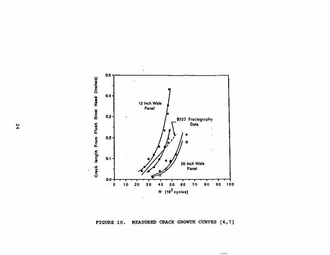
FIGURE 10. MEASURED CRACK GROWTH CURVES [6, 7]

19 t- \\ \ \ \
~ HARTMAN 181- INITIATION ~ ,,, ' FAIUJRE (RIVETED)
\ '
17 1-\ \
15 PERCENTILE . \ H
16 ~ \ U) :::=.::: 25 PERCENTILe \ - \
w 50 PERCENTILE \
(.!) 15 (AVERAGE) \
z \ < a: \
N U) \
U1 U) 14 ' w ALOHA \ a: 1- (ADJUSTED FOR CONSTANT \
U) 13 ' AMPLITUDE) \ \
\
121- \ \ . \ \
' 111- \ \ \ \
'
2.5 3.0 3.5 4.0 4.5 5.0 5.5 6.0 6.5 LOG (N) (CYCLES)
FIGURE 11. S-N CURVES USED IN ANALYSIS

IV 0\
9
8
0 UJ 7 ~ CJ < 5 6 en UJ
c5 5 :::c ~ z 4 UJ CJ a: ~ 3
2
1
10
MAXIMUM DlFFERENTIAL PRESSURE IN psi
9 8.5 8 7.5
I I 1/ i;~~ 1
1
// // ·-.,./
7 I I
I I
I
20 30 40 50 60 70 N (1000 FLIGHTS)
80 90
FIGURE 12. OPTIMISTIC CASE WHERE ALOHA BELONGS TO LOWER 15 PERCENTILE

N -..J
MAXIMUM DIFFERENTIAL PRESSURE IN psi
9
sr 9 8.5 9 7.5 7 Cl w 7 ::.! I u <( a: I u 6 en I w 5 5 I :r: t- I z w 4 I u a:
I w a... 3
I 21- I I I I I
I 11- I I I / /
/ / Kz<: ,cr; se: I ,..::::;:: I
7.5 15.0 22.5 30.0 37.5 45.0 52.5 60.0 67.5 N (1000 FLIGHTS)
FIGURE 13. CASE IN WHICH ALOHA BELONGS TO LOWER 25 PERCENTILE
gr MAXIMUM DIFFERENTIAL PRESSURE IN psi
8 0
7 I 9 8.5 8 7.5 7 lU ~ u <
I I a:
I u
6 I U) ' I lU
I I .....J 0 5 I ::r: I lV ..... ' I I
I ()) z
4 I
I lU
I
I u
I I a: lU
I I a.. 3 I I
I 21- I I I I / 1
/ 1._ I l / / /
5 10 15 20 25 30 35 40 45 N ( 1000 FLIGHTS)
FIGURE 14. CONSERVATIVE CASE WHERE ALOHA IS AVERAGE

g· LOWER PERCENTILE TO WHICH ALOHA BELONGS TO:
8
Cl
~ 7 50 25 15 I c..J
<( a:
I c..J 6 en I LU
c5 5 I :c t.J t-
I I "' ffi 4 I c..J
a: I LU I
a. 3 I I
21- I / I I. 11- ./ / /
/ --./
I d"" r= ....,..-5 10 15 20 25 30 35 40 45
N (1000 FLIGHTS)
FIGURE 15. THREE CASES FOR DIFFERENTIAL PRESSURE OF 8 psi

w 0
0.9
0.8
0.7 -:c u ~ 0.6 -w ~ 0.5 en ~ u 0.4 <( a: u
0.3
0.2
0.1
LINK-UP (FAILURE}
10 20
I
30 40 50 60 70 LOCATION (HOLE NUMBER)
80 90
FIGURE 16. FINAL CRACK SIZES AT ALL LOCATIONS - SAME CASE AS IN FOLLOWING FIGURE - SOLID LINE: LEFT CRACK; DASH-DOT: RIGHT CRACK

w ....
-
0.9 ~
0.8 :-
0.7 -..... gs 0.6 .... .
CD
~ 0.5 ~ a.
-%. 0.4 ~
:-
u
0.3 -
0.2 -
0.1 -I
10 I
20 l I I I I
30 40 50 60 70 LOCATION (HOLE NUMBER)
I I
80 90
FIGURE 17. CUMULATIVE PROBABILITY OF DETECTION PER LOCATION - SOLID LINE: EDDY CURRENT; DASH-DOT LINE: VISUAL INSPECTION INTERVAL 3000 CYCLES; TYPICAL CASE

-rn Q) .c: 0 .5 -.c: -C)
w N
c: Q) ..J ..lll: 0 ~ ()
N = 64,820 cycles 0.5--------------------.,.-___,
0.4
0.3
0.2
0.1
0.0 I I
1
Panel: 12-F-1-2
Tear Strap
2 3 4
• Left Side of Rivet
f1 Right Side of Rivet
5 6 7 8
Rivet Number (Position Along Joint)
9
Tear Strap
10 11 12
FIGURE 18. MEASURED CRACK SIZES AT FAILURE [6,7]

w w
N = 43,400 flights
0.3 .
-(/) Q)
£ 0.2 r::
:.::, .r:: -C) r:: Q) -1 ~
~ 0.1 '-
(.)
Frame Location
• Left Side of Rivet
II Right Side of Rivet
Frame Location
0.0 I W·I-W
1 2 3 4 56 7 8 91011121314151617181920212223242526272829303132333435
Rivet Number (Position Along Joint)
FIGURE 19. SIZES OF DETECTED MSD IN AIRCRAFT [6,7]

w oil-
0. 9 1-
0. 8 1-
0. 7 1-
-:c t.J ~ 0.61--~ 0.51-H en
[5 o.41-<( a: t.J 0.31-
0. 2 1-
0. 1 t-
I I I I I I J I • _j__ I I I I
10 20 30 40 50 60 70 80 90 LOCATION (HOLE NUMBER)
FIGURE 20. SIZE DISTRIBUTION WHEN LARGEST CRACK IS 0.1 INCH

w U1
9
8
s: ~ 7 ~
~
0 6 . 0 -UJ N ~ U)
::::.::: c...J <( a: u
5
4
3
2 4 6 8 10 12 14 16
LARGEST CRACK
NUMBER OF CRACKS
2~------
1
2 4 6 8 10 12 14 16 N ( 1000 CYCLES)
(1000 CYCLES) 18
(# OF CRACKS)
9
8
7
6
5
4
3
2
1
18
FIGURE 21.NUMBER OF CRACKS AND SIZE OF LARGEST CRACK - EXAMPLE OF STATISTICALLY ARBITRARY CASE

w 0\
-::c u z H -UJ N H en :::.=:: u <( a: u
0.9
0.8
0.7
0.6
0.5
0.4
0.3
0.2
0.1
10 20 30 40 50 60 70 LOCATION (HOLE NUMBER)
80 90
FIGURE 22. SIZE DISTRIBtrriON WHEN LARGEST CRACK IS 0.1 INCH

w 0)
45
~) :I: t!l H
ti 35 0 0 0 30 -c-4 -53 25
I ~ u <(
5 20 N
0 15 f-
UJ lL. 10 H ....J
5
ALOHA IS 25 PERCENTILE ~ 6l ALOHA IS 15 PERCENTILE
ALOHA IS AVERAGE
5.5 6.0 6.5 7.0 7.5 8.0 8.5 9.0 9.5 MAX. PRESSURE DIFF. (psi)
FIGURE 24. SUMMARY OF RESULTS - LIFE UNTIL 2 PERCENT CRACKED

-en I-:::r: (.!) H _J l1..
0 0 0 ~ -Cl l.U ~ u w <t
-..I a: u ~
0 I-
l.U l1.. H _J
ALOHA IS 15 PERCENTILE . 45
40
35 I ALOHA IS 25 PERCENTILE
30
25
20
15
10
5
I ALOHA IS AVERAGE
5.5 6.0 6.5 7.0 7.5 8.0 8.5 9.0 9.5 MAX. PRESSURE DIFF. {psi)
FIGURE 23. SUMMARY OF RESULTS - LIFE UNTIL 1 PERCENT CRACKED
-en 1--::c (!) H .....J l1...
0 0 0 ~ ........
CJ UJ
w ~ \0 u
<t a: u N
0 1--
UJ l1... H .....J
67.5 L
60.0
52.51
45.0
37.5
30.0 1-
22.5
15.0
7.5
ALOHA IS 15 PERCENTILE
ALOHA IS 25 PERCENTILE
ALOHA IS AVERAGE
5.5 6.0 6.5 7.0 7.5 8.0 8.5 9.0 9.5 MAX. PRESSURE DIFF. (psi)
FIGURE 25. SUMMARY OF RESULTS - LIFE UNTIL 5 PERCENT CRACKED

~ 0
45
-U) f- 40 :c (!) H _J 35 lL..
0 0 0 30 ~ -Cl 25 UJ ~ u <t c: 20 u ~
0 15 f-
UJ lL.. 10 H _J
5
I
I
2 PER CENT CRACKED it.. 5 PER CENT CRACKED
1 PER CENT CRACKED
5.5 6.0 6.5 7.0 7.5 8.0 8.5 9.0 9.5 MAX. PRESSURE DIFF. ~si)
FIGURE 26. SUMMARY OF RESULTS - CASE WHERE ALOHA BELONGS TO LOWER 25 PERCENTILE

,. ....
135 r MAXIMUM DIFFERENTIAL PRESSURE (psi)
9 8.5 8 7.5 7 120 1- I
- I 5 105 z I H
~ 90 I 0 0
I . - 75 I UJ N H
I en 60 ~ I u <( c: 45 u
30
15
10 20 30 40 50 60 70 80 90 LIFE {1000 FLIGHTS)
FIGURE 27. CRACK GROWTH; RUN ID: 17685 AT DIFFERENT MAXIMUM PRESSURES STARTING AT 0.005 INCH

90 -~ t-::J: 80 (.!) H ....J
~DIFFERENTIAL PRESSURE FROM TOP TO BOTTOM: LL
0 70 0 7; 7.5; 8; 8.5; AND 9 psi 0 ....... ..__
60 ~ u <(
50 a: \ u ,e. z ,,, "'
H 40 C\J ~" .......
~' .
0 30 ',, 0 \ ·,"'-.. ,, t-
'~,, UJ 20 ' .. , .... ~ LL .......... ........... ............. H .......... , ............................ ....J __ .............. .....:::.. ..........
10 ---...........:: .. ~ .... ---.....;;: .. ~.... ----::::::...-.;.........::::-~
-=-~iii
15 30 45 60 75 90 105 120 135 ASSUMED EIF (0.001 INCH)
FIGURE 28. LIFE UNTIL 0.12 INCH CRACK AS A FUNCTION OF ASSUMED EQUIVALENT INITIAL FLAW (EIF) SIZE