Byungjin Cho

A Simulation study on Interference inCSMA/CA Ad-Hoc Networks using PointProcess

Faculty of Electronics, Communications and Automation

Thesis submitted for examination for the degree of Master of

Science in Technology.

Espoo 31.12.2010

Thesis supervisor:

Prof. Riku Jäntti

Thesis instructor:

PhD. June Hwang

A’’ Aalto UniversitySchool of Scienceand Technology

aalto university

school of science and technology

abstract of the

master’s thesis

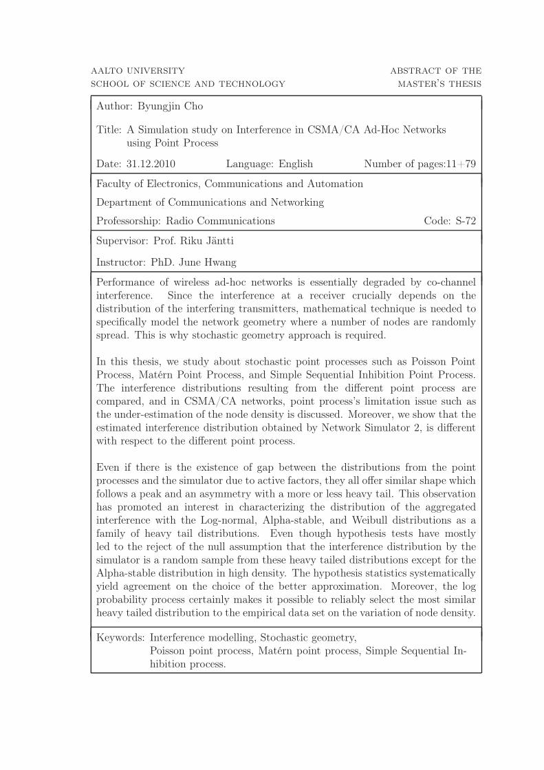
Author: Byungjin Cho

Title: A Simulation study on Interference in CSMA/CA Ad-Hoc Networksusing Point Process

Date: 31.12.2010 Language: English Number of pages:11+79

Faculty of Electronics, Communications and Automation

Department of Communications and Networking

Professorship: Radio Communications Code: S-72

Supervisor: Prof. Riku Jäntti

Instructor: PhD. June Hwang

Performance of wireless ad-hoc networks is essentially degraded by co-channelinterference. Since the interference at a receiver crucially depends on thedistribution of the interfering transmitters, mathematical technique is needed tospecifically model the network geometry where a number of nodes are randomlyspread. This is why stochastic geometry approach is required.

In this thesis, we study about stochastic point processes such as Poisson PointProcess, Matérn Point Process, and Simple Sequential Inhibition Point Process.The interference distributions resulting from the different point process arecompared, and in CSMA/CA networks, point process’s limitation issue such asthe under-estimation of the node density is discussed. Moreover, we show that theestimated interference distribution obtained by Network Simulator 2, is differentwith respect to the different point process.

Even if there is the existence of gap between the distributions from the pointprocesses and the simulator due to active factors, they all offer similar shape whichfollows a peak and an asymmetry with a more or less heavy tail. This observationhas promoted an interest in characterizing the distribution of the aggregatedinterference with the Log-normal, Alpha-stable, and Weibull distributions as afamily of heavy tail distributions. Even though hypothesis tests have mostlyled to the reject of the null assumption that the interference distribution by thesimulator is a random sample from these heavy tailed distributions except for theAlpha-stable distribution in high density. The hypothesis statistics systematicallyyield agreement on the choice of the better approximation. Moreover, the logprobability process certainly makes it possible to reliably select the most similarheavy tailed distribution to the empirical data set on the variation of node density.

Keywords: Interference modelling, Stochastic geometry,Poisson point process, Matérn point process, Simple Sequential In-hibition process.

Acknowledgements

This thesis is based on the work that was carried out in the Communications Lab-oratory, Aalto university, from June 2010 to December 2010.

First, I wish to express my sincere gratitude to my thesis supervisor ProfessorRiku Jäntti and instructor Ph.D June Hwang for giving me this opportunity to carryout this work. I would like to thank Professor Riku Jäntti for his continuous encour-agement, professional advices, and constant support during the course of this thesis.I would like to thank my thesis advisor Ph.D June Hwang for his guidance through-out my work for this thesis. His wide knowledge and his logical way of thinkinghave been of great value for me. This work would not have been possible withouthis insightful comments and thoughts. His constant encouragement and his strivefor excellence make working with him a rewarding experience. The discussion i hadwith Professor Riku Jäntti and Ph.D June Hwang, their comments and suggestionshave greatly contributed to the quality of the thesis.

I wish to express my appreciation to my colleagues and friends, Cho’s family,Sungin Cho, Kyunghyun Cho, and Eunah Cho for their help during the work. Theirincredible support carried me through the roughest times and have helped to keepme sane with a diversity of liquor supply. I also would like to thank all my friendsin Finland and in South Korea, for their genuine friendship.

Finally, the deepest gratitude goes to my family for their love and support. Ihaven’t got enough words for thanking my parents for their encouragement duringmy whole life.

Otaniemi, 31.12.2010 Byungjin Cho

iii

Contents

Acknowledgements iii

Contents iv

List of Abbreviations vi

List of Symbols vii

List of Figures x

List of Tables xi

1 Introduction 1

1.1 Motivation and Related Work . . . . . . . . . . . . . . . . . . . . . . 11.2 Scope . . . . . . . . . . . . . . . . . . . . . . . . . . . . . . . . . . . 21.3 Contribution and Organization . . . . . . . . . . . . . . . . . . . . . 2

2 Preliminaries 4

2.1 Spatial Point Process . . . . . . . . . . . . . . . . . . . . . . . . . . . 42.1.1 Poisson Point Process . . . . . . . . . . . . . . . . . . . . . . 5

2.2 Shot Noise . . . . . . . . . . . . . . . . . . . . . . . . . . . . . . . . . 52.3 Heavy tailed distribution . . . . . . . . . . . . . . . . . . . . . . . . . 7

2.3.1 Alpha-stable distribution . . . . . . . . . . . . . . . . . . . . . 72.3.2 Log-normal and Weibull distributions . . . . . . . . . . . . . . 9

3 SYSTEM MODEL 12

3.1 Propagation Channel Model . . . . . . . . . . . . . . . . . . . . . . . 123.2 Medium Access Control . . . . . . . . . . . . . . . . . . . . . . . . . 133.3 Interference Models for PPP spatial node distribution . . . . . . . . . 143.4 Interference Models for Exclusively Deployed Nodes . . . . . . . . . . 16

3.4.1 Poisson Point Process with modified density . . . . . . . . . . 163.4.2 Matérn Point Process . . . . . . . . . . . . . . . . . . . . . . . 173.4.3 Simple Sequential Inhibition . . . . . . . . . . . . . . . . . . . 18

3.5 Challenge of Point Processes . . . . . . . . . . . . . . . . . . . . . . . 19

iv

v

4 Simulation Results and Analysis 21

4.1 NS-2 Simulation Set-up . . . . . . . . . . . . . . . . . . . . . . . . . . 214.2 Theoretical and Experimental values of Interference distribution . . . 254.3 Process Comparisons . . . . . . . . . . . . . . . . . . . . . . . . . . . 264.4 Difference with NS-2 results . . . . . . . . . . . . . . . . . . . . . . . 284.5 Statistical Significance Test . . . . . . . . . . . . . . . . . . . . . . . 32

4.5.1 Hypothesis Checking Technique . . . . . . . . . . . . . . . . . 324.5.2 process comparison with NS2 result . . . . . . . . . . . . . . . 324.5.3 Extrapolation Analysis . . . . . . . . . . . . . . . . . . . . . . 36

5 Conclusions and Future Work 41

5.1 Conclusions . . . . . . . . . . . . . . . . . . . . . . . . . . . . . . . . 415.2 Possible Future Work . . . . . . . . . . . . . . . . . . . . . . . . . . . 42

Bibliography 44

APPENDICES 47

A Matlab Codes 47

A.1 Main.m . . . . . . . . . . . . . . . . . . . . . . . . . . . . . . . . . . 47A.2 Extrapolation2.m . . . . . . . . . . . . . . . . . . . . . . . . . . . . . 55

B NS2 Scripts 64

B.1 Main.tcl . . . . . . . . . . . . . . . . . . . . . . . . . . . . . . . . . . 64B.2 Scenario.tcl . . . . . . . . . . . . . . . . . . . . . . . . . . . . . . . . 68B.3 Traffic.tcl . . . . . . . . . . . . . . . . . . . . . . . . . . . . . . . . . 70B.4 Trace.awk . . . . . . . . . . . . . . . . . . . . . . . . . . . . . . . . . 73B.5 Poisson.c . . . . . . . . . . . . . . . . . . . . . . . . . . . . . . . . . . 77

List of Abbreviations

NS Network SimulatorPP Point ProcessPPP Poisson Point ProcessPPPmd Poisson Point Process with modified densityMPP Matern Point ProcessSSI Simple Sequential InhibitionCSMA Carrier Sensing Multiple AccessCA Collision AvoidanceMAC Medium Access ControlCCA Clear Channel AssessmentRTS Request-To-SendCTS Clear-To-SendPDF Probability Density FunctionCDF Cumulative Distribution Functioniff if and only ifi.i.d Independent and Identically DistributedCS Carrier SenseDCF Distributed Coordination Functionchi2gof Chi-square goodness-of-fitkstest Kolmogorov-Smirnov TestSINR Signal to Interference and Noise RatioCLT Central Limit TheoremAs Alpha-stable distributionLn Log-normal distributionWb Weibull distributionPLCP Physical Layer Convergence Procedure

vi

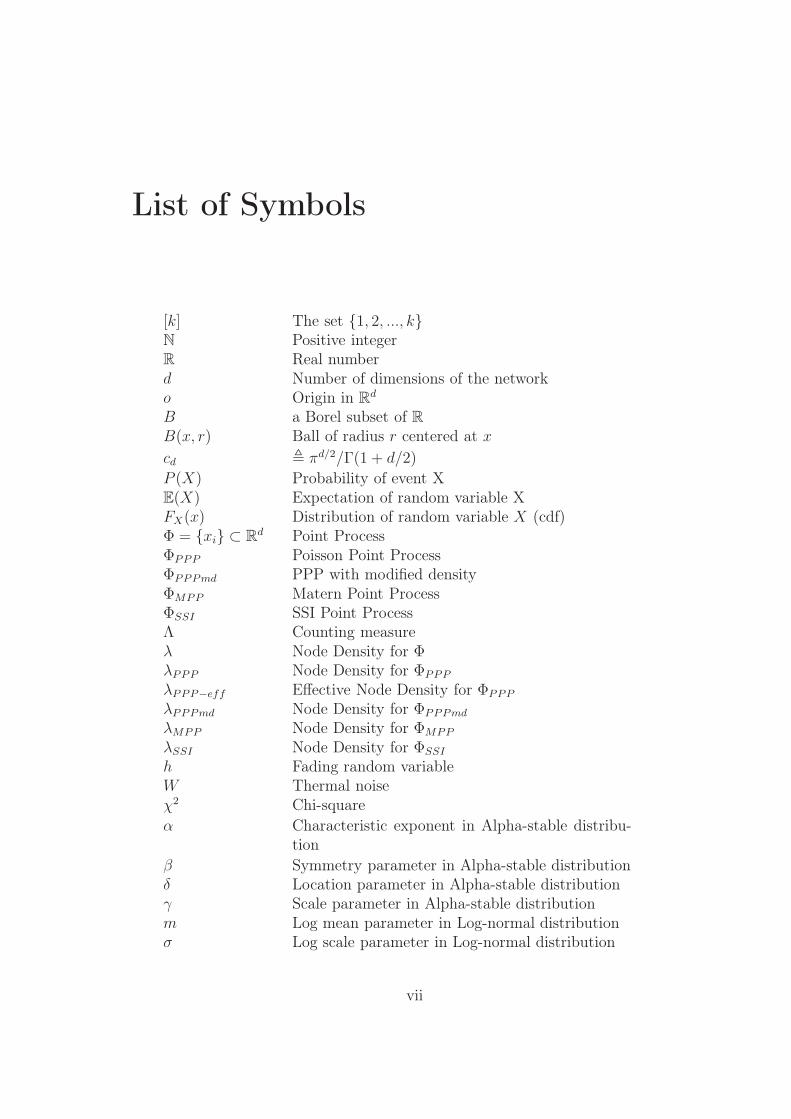
List of Symbols

[k] The set {1, 2, ..., k}N Positive integerR Real numberd Number of dimensions of the networko Origin in R

d

B a Borel subset of RB(x, r) Ball of radius r centered at x

cd , πd/2/Γ(1 + d/2)

P (X) Probability of event XE(X) Expectation of random variable XFX(x) Distribution of random variable X (cdf)Φ = {xi} ⊂ R

d Point ProcessΦPPP Poisson Point ProcessΦPPPmd PPP with modified densityΦMPP Matern Point ProcessΦSSI SSI Point ProcessΛ Counting measureλ Node Density for ΦλPPP Node Density for ΦPPP

λPPP−eff Effective Node Density for ΦPPP

λPPPmd Node Density for ΦPPPmd

λMPP Node Density for ΦMPP

λSSI Node Density for ΦSSI

h Fading random variableW Thermal noiseχ2 Chi-square

α Characteristic exponent in Alpha-stable distribu-tion

β Symmetry parameter in Alpha-stable distributionδ Location parameter in Alpha-stable distributionγ Scale parameter in Alpha-stable distributionm Log mean parameter in Log-normal distributionσ Log scale parameter in Log-normal distribution

vii

viii

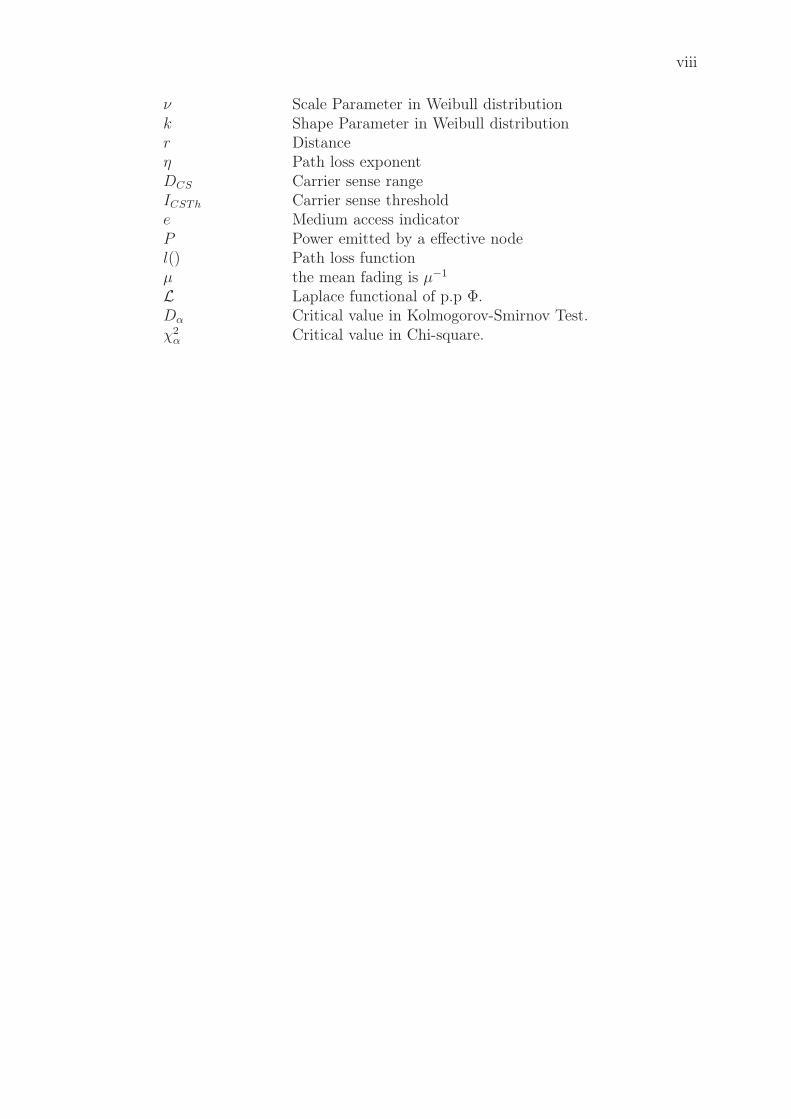
ν Scale Parameter in Weibull distributionk Shape Parameter in Weibull distributionr Distanceη Path loss exponentDCS Carrier sense rangeICSTh Carrier sense thresholde Medium access indicatorP Power emitted by a effective nodel() Path loss functionµ the mean fading is µ−1

L Laplace functional of p.p Φ.Dα Critical value in Kolmogorov-Smirnov Test.χ2α Critical value in Chi-square.

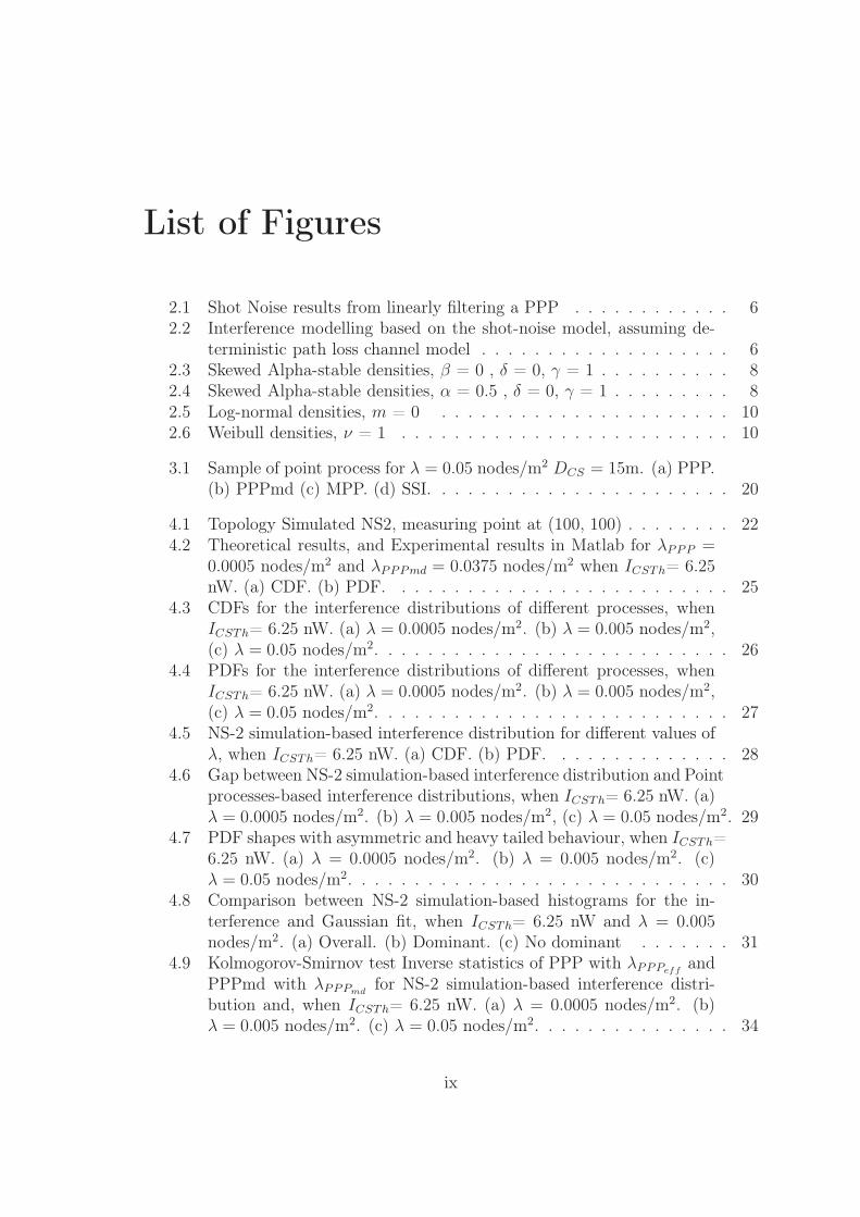
List of Figures

2.1 Shot Noise results from linearly filtering a PPP . . . . . . . . . . . . 62.2 Interference modelling based on the shot-noise model, assuming de-

terministic path loss channel model . . . . . . . . . . . . . . . . . . . 62.3 Skewed Alpha-stable densities, β = 0 , δ = 0, γ = 1 . . . . . . . . . . 82.4 Skewed Alpha-stable densities, α = 0.5 , δ = 0, γ = 1 . . . . . . . . . 82.5 Log-normal densities, m = 0 . . . . . . . . . . . . . . . . . . . . . . 102.6 Weibull densities, ν = 1 . . . . . . . . . . . . . . . . . . . . . . . . . 10

3.1 Sample of point process for λ = 0.05 nodes/m2 DCS = 15m. (a) PPP.(b) PPPmd (c) MPP. (d) SSI. . . . . . . . . . . . . . . . . . . . . . . 20

4.1 Topology Simulated NS2, measuring point at (100, 100) . . . . . . . . 224.2 Theoretical results, and Experimental results in Matlab for λPPP =

0.0005 nodes/m2 and λPPPmd = 0.0375 nodes/m2 when ICSTh= 6.25nW. (a) CDF. (b) PDF. . . . . . . . . . . . . . . . . . . . . . . . . . 25

4.3 CDFs for the interference distributions of different processes, whenICSTh= 6.25 nW. (a) λ = 0.0005 nodes/m2. (b) λ = 0.005 nodes/m2,(c) λ = 0.05 nodes/m2. . . . . . . . . . . . . . . . . . . . . . . . . . . 26

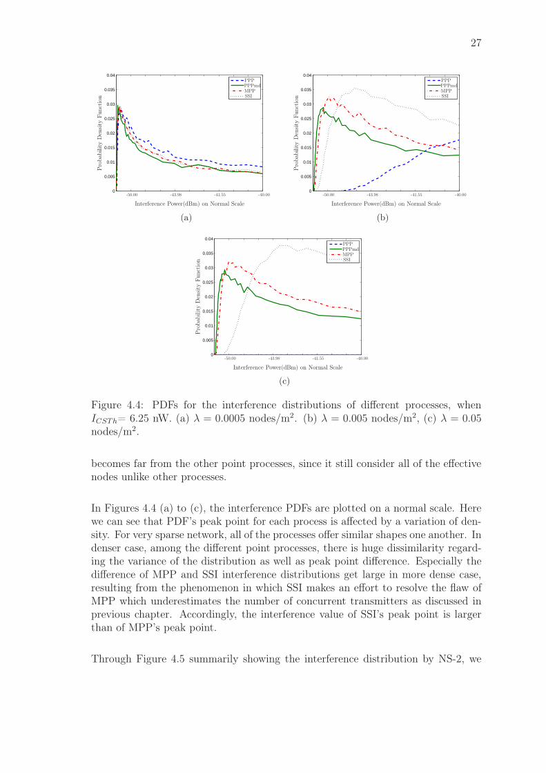
4.4 PDFs for the interference distributions of different processes, whenICSTh= 6.25 nW. (a) λ = 0.0005 nodes/m2. (b) λ = 0.005 nodes/m2,(c) λ = 0.05 nodes/m2. . . . . . . . . . . . . . . . . . . . . . . . . . . 27

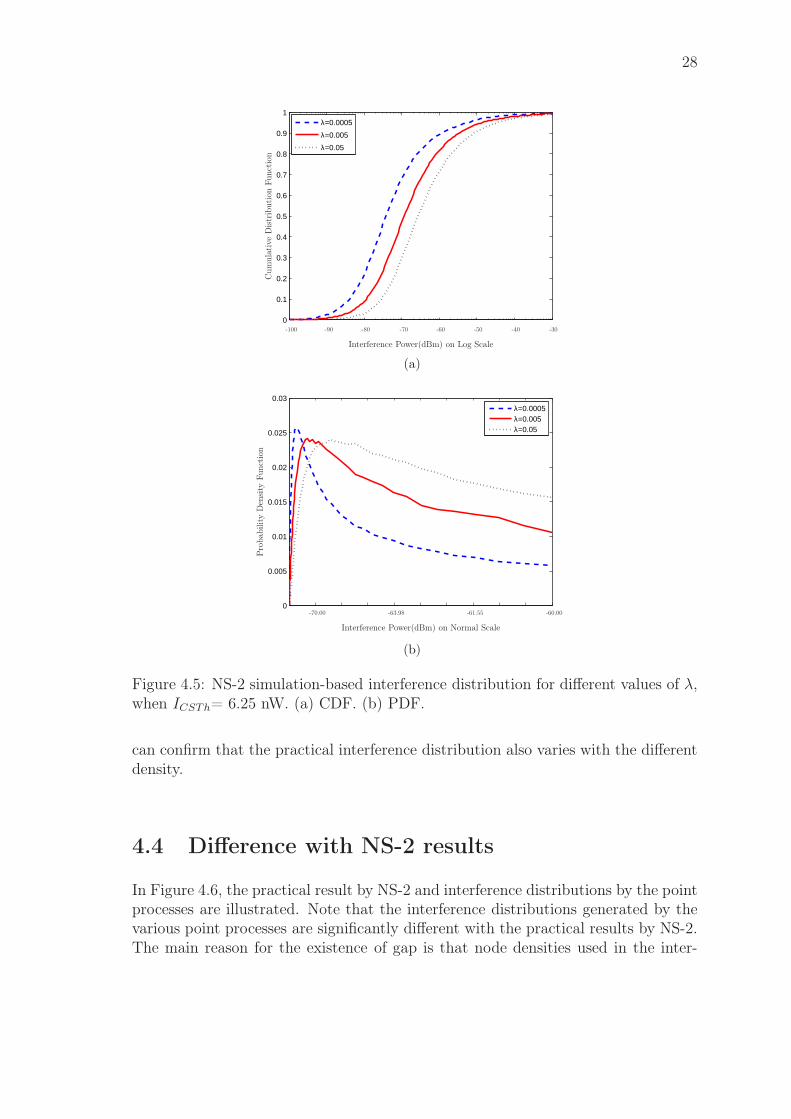
4.5 NS-2 simulation-based interference distribution for different values ofλ, when ICSTh= 6.25 nW. (a) CDF. (b) PDF. . . . . . . . . . . . . . 28

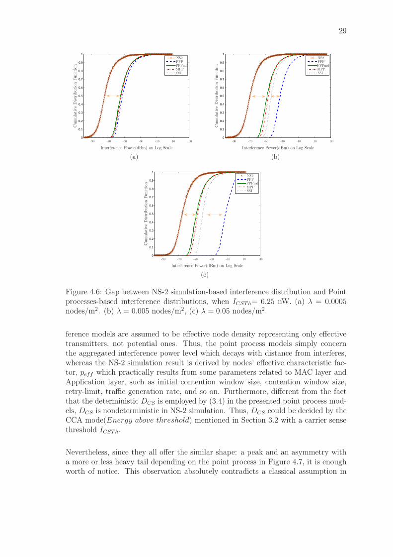
4.6 Gap between NS-2 simulation-based interference distribution and Pointprocesses-based interference distributions, when ICSTh= 6.25 nW. (a)λ = 0.0005 nodes/m2. (b) λ = 0.005 nodes/m2, (c) λ = 0.05 nodes/m2. 29

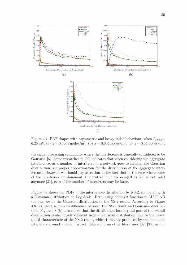
4.7 PDF shapes with asymmetric and heavy tailed behaviour, when ICSTh=6.25 nW. (a) λ = 0.0005 nodes/m2. (b) λ = 0.005 nodes/m2. (c)λ = 0.05 nodes/m2. . . . . . . . . . . . . . . . . . . . . . . . . . . . . 30

4.8 Comparison between NS-2 simulation-based histograms for the in-terference and Gaussian fit, when ICSTh= 6.25 nW and λ = 0.005nodes/m2. (a) Overall. (b) Dominant. (c) No dominant . . . . . . . 31

4.9 Kolmogorov-Smirnov test Inverse statistics of PPP with λPPPeffand

PPPmd with λPPPmdfor NS-2 simulation-based interference distri-

bution and, when ICSTh= 6.25 nW. (a) λ = 0.0005 nodes/m2. (b)λ = 0.005 nodes/m2. (c) λ = 0.05 nodes/m2. . . . . . . . . . . . . . . 34

ix

x

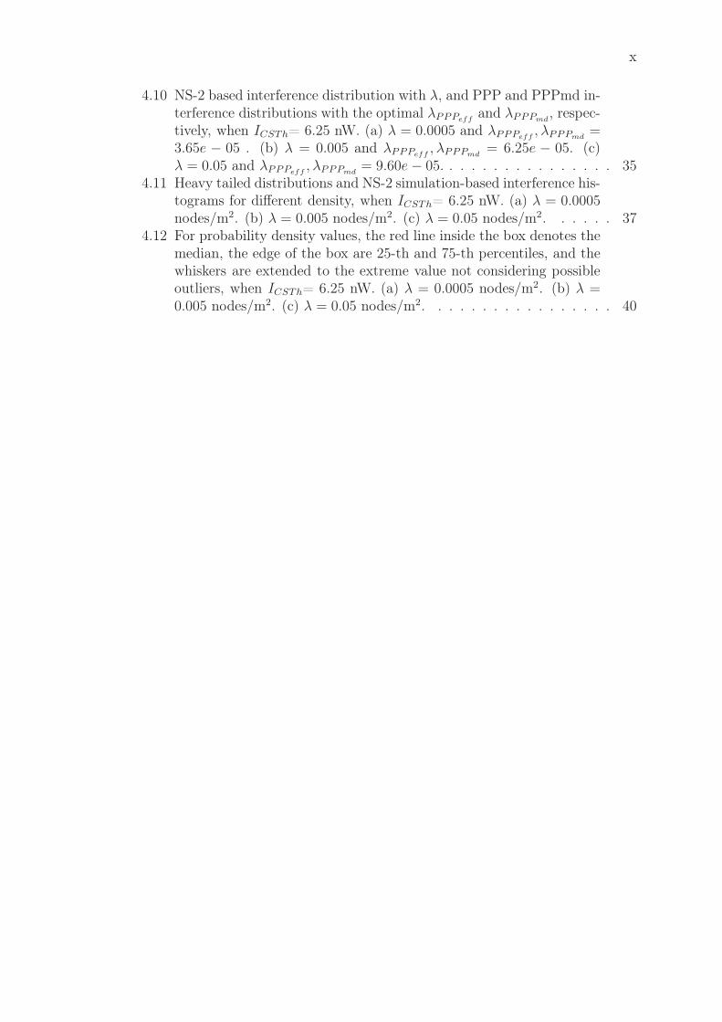
4.10 NS-2 based interference distribution with λ, and PPP and PPPmd in-terference distributions with the optimal λPPPeff

and λPPPmd, respec-

tively, when ICSTh= 6.25 nW. (a) λ = 0.0005 and λPPPeff, λPPPmd

=3.65e − 05 . (b) λ = 0.005 and λPPPeff

, λPPPmd= 6.25e − 05. (c)

λ = 0.05 and λPPPeff, λPPPmd

= 9.60e− 05. . . . . . . . . . . . . . . . 354.11 Heavy tailed distributions and NS-2 simulation-based interference his-

tograms for different density, when ICSTh= 6.25 nW. (a) λ = 0.0005nodes/m2. (b) λ = 0.005 nodes/m2. (c) λ = 0.05 nodes/m2. . . . . . 37

4.12 For probability density values, the red line inside the box denotes themedian, the edge of the box are 25-th and 75-th percentiles, and thewhiskers are extended to the extreme value not considering possibleoutliers, when ICSTh= 6.25 nW. (a) λ = 0.0005 nodes/m2. (b) λ =0.005 nodes/m2. (c) λ = 0.05 nodes/m2. . . . . . . . . . . . . . . . . 40

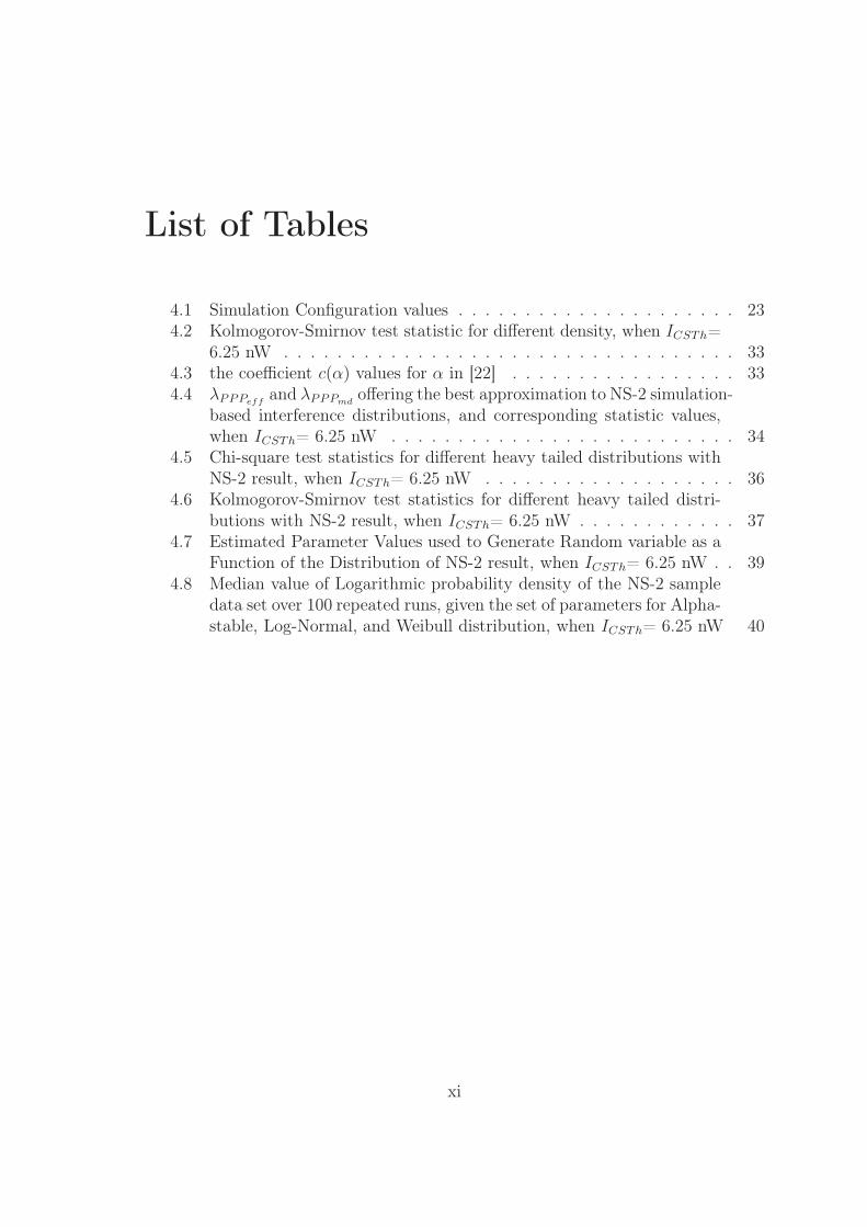
List of Tables

4.1 Simulation Configuration values . . . . . . . . . . . . . . . . . . . . . 234.2 Kolmogorov-Smirnov test statistic for different density, when ICSTh=

6.25 nW . . . . . . . . . . . . . . . . . . . . . . . . . . . . . . . . . . 334.3 the coefficient c(α) values for α in [22] . . . . . . . . . . . . . . . . . 334.4 λPPPeff

and λPPPmdoffering the best approximation to NS-2 simulation-

based interference distributions, and corresponding statistic values,when ICSTh= 6.25 nW . . . . . . . . . . . . . . . . . . . . . . . . . . 34

4.5 Chi-square test statistics for different heavy tailed distributions withNS-2 result, when ICSTh= 6.25 nW . . . . . . . . . . . . . . . . . . . 36

4.6 Kolmogorov-Smirnov test statistics for different heavy tailed distri-butions with NS-2 result, when ICSTh= 6.25 nW . . . . . . . . . . . . 37

4.7 Estimated Parameter Values used to Generate Random variable as aFunction of the Distribution of NS-2 result, when ICSTh= 6.25 nW . . 39

4.8 Median value of Logarithmic probability density of the NS-2 sampledata set over 100 repeated runs, given the set of parameters for Alpha-stable, Log-Normal, and Weibull distribution, when ICSTh= 6.25 nW 40

xi

Chapter 1

Introduction

1.1 Motivation and Related Work

Spectral Resource reuse technique has been studied over the last decade to improvethroughput capacity of wireless systems such as adhoc and sensor networks andcellular networks. While spectral resource reuse leads to capacity improvement, itcauses co-channel interference, one of the key factors degrading overall performancein wireless communications. Therefore, a better understanding of the effects of in-terference on the performance of wireless communication system demanding a moreaggressive utilization of spectral resources, for instance the newly emerged CognitiveRadio system, has become an important critical issue, motivating the developmentof more accurate interference models.

An interference model can be regarded as a mixture of different sub-models such aspropagation model, interferers spatial distribution model, network operation model,and traffic model, each of which could be employed as a deterministic or randomprocess, depending on the scenario considered. Since the accumulative interferencegenerated by concurrent transmitting nodes overwhelmingly depends on nodes’ lo-cation and the geometry information plays an important role in the interferencemodelling process, this thesis focuses on effective(active) interferers spatial distri-bution model, while the other components are taken into consideration under someassumptions which will be presented later.

Significantly unequal to infrastructure based wireless systems, there is high level ofuncertainty in adhoc network which is formed by a number of nodes randomly spreadover a large area. The position of the nodes are usually unknown, and hence theinterference situation cannot be controlled by careful network planning. Therefore,a stochastic approach is required to properly describe the interference distribution.

In fact, a myriad of the spatial distribution models of the nodes have been suggested

1

2

with using stochastic geometry tool which enable to make on average all realizationsof the network whose nodes are placed according to some distribution, such as Pois-son Point Process [1] which is analytically convenient and leads to some insightfulresults with its independence property.

However, in practice, this process is not accurate anymore for a CSMA/CA protocolin which a spatial correlation between nodes is introduced by medium access policyto avoid collisions. In recent works [2] [3], some researchers already made objectionto this issue by modifying the initial Poisson process, so called hardcore models [4]where a minimum node separation is properly applied.

Nevertheless, they are still in their infancy due to some flaws [20] such as the spatialanomaly and thus an underestimation of the interference level. In [5], the use of analternate model, referred to as the Simple Sequential Inhibition (SSI) point processwas proposed. However, they do not provide the practical results by simulator.

1.2 Scope

In this thesis, we first introduce different point processes, and then compare theinterference distributions resulting from these different ones. Moreover, we pointout how different they are with practical simulation results induced by NS-2, andcheck whether the simulated interference could be extrapolated by considered dis-tributions such as a log-normal or an alpha-stable distribution, thereby giving abenefit to engineers and researchers looking for appropriately approximated one topractical interference distribution as well as interference models in some particularscenario.

1.3 Contribution and Organization

This thesis is organized as follows.

Chapter 2 contains a description of the concepts that are essential for understandingthe analysis that is to follow in the remaining of this thesis. The concepts of Pointprocess and shot noise are introduced and a short introduction to heavy taileddistributions is presented.

In Chapter 3, the system model is introduced. Channel and MAC models usedfor this thesis are described. With results on Laplace functional of Poisson shotnoise processes, some interference models for CSMA/CA network are introduced,and limitations for these models are discussed in detail.

3

Chapter 4 provides the results that are obtained by simulation tool, NS2. Based onthe practical results, analysis for the interference models is discussed, and we testan extrapolation with the distribution resulting from NS-2.

Finally, conclusions and possible future research directions are discussed in Chapter5.

Chapter 2

Preliminaries

In this chapter, we give a thorough background description on the concepts thatare essential for understanding the analysis that follows in the remaining of thisthesis. We begin in Section 2.1 with Point process and shot noise concept whichare needed for stochastic geometry. Furthermore, in Section 2.2, we provide a shortintroduction to Alpha-stable, Log-normal, and Weibull distributions, which we willencounter in analysis of simulation result.

2.1 Spatial Point Process

In a case that every node has a single antenna and only a single channel is consid-ered, interference is referred to as co-channel interference. In the statistical analysisof interference in wireless networks, the aggregate interference is the incoherent sumof individual interfering signals. The statistical characteristics of interference ob-viously depend on the statistics of the individual interfering signals. One of themain factors invoking the randomness of the individual interfering signals could bethe distances between the location at which interference is received and interferingnodes. Since the distances influence on the mean power levels of interfering sig-nals, these distances play an important role in the modelling process. Therefore,a stochastic model for the node locations (i.e., a spatial point process) is needed.Spatial point processes are the generalization of point processes indexed by timeto higher dimensions, such as 2-D space. Stochastic geometry provides the toolsto analyse important quantities such as interference distributions and link outages,and thus permits statistical statements about network performance [2, 3]. It shallallow us to focus on interference distributions in this thesis.

Formally, a point process Φ is viewed as a set of random points with a certain prob-ability in a space E, where it is the Euclidean space R

d of dimension d ≧ 1. Theintensity measure Λ of a point process Φ is equal to the average number of pointsin a set B ⊂ R

d, and could be defined as:

4

5

Λ(B) = E(Φ(B)) for Borel B. (2.1)

Here are a few basic definition concerning point processes on some Euclidean spaceR

d:

• Stationary: xi and xi + x have same distribution.

• Isotropy: the same holds for all rotations about the origin.

• Motion-invariance: Stationary plus isotropy.

2.1.1 Poisson Point Process

Due to its analytical tractability and practical appeal in situations where transmit-ters and/or receivers are located or move around randomly over a large area, thePoisson point process (PPP) has been by far the most popular spatial model. LetΛ be a locally finite measure on some metric space E, the Euclidean space R

d. Apoint processes Φ is Poisson on E if

• For all disjoint subsets {A1, ..., An} ⊂ Rd, the random variable Φ(A1), ...,Φ(An)

are independent.

• For all sets A ⊂ Rd, the random variables Φ(A) are Poisson.

The density of nodes in a unit area is λ, and so the average number of nodes in anarea A is Λ(A) = λA.

2.2 Shot Noise

Stochastic geometry combines the shot noise process with stochastic point processeswhich are drawn from a statistical distribution, most commonly the PPP as justdiscussed. We begin this section by reviewing some basic concepts on shot noisetheory, considering the one dimensional case at first and the higher dimensional onefor the interference modelling.

Let us consider a memoryless linear filter with stochastic impulse response functionf(h, t), where h is a random variable, and assume this filter is excited by a train ofimpulses at instants tj derived from a one-dimensional Poisson Point process withintensity(density) λ.

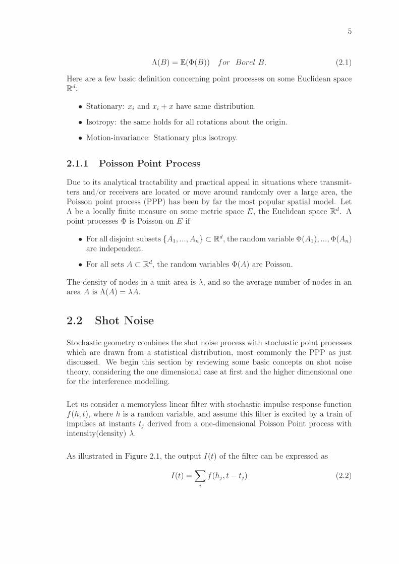
As illustrated in Figure 2.1, the output I(t) of the filter can be expressed as

I(t) =∑

i

f(hj , t− tj) (2.2)

6

S o noise

Linear Fil er ( , )

PPP

t

t

t

tt

t

h

h

f

Figure 2.1: Shot Noise results from linearly filtering a PPP

where {hj} is independent of tj and a random sequence, whose elements are drawnfrom a common distribution. The output I(t) is said to be the shot noise associatedwith the Poisson Point process with intensity λ.

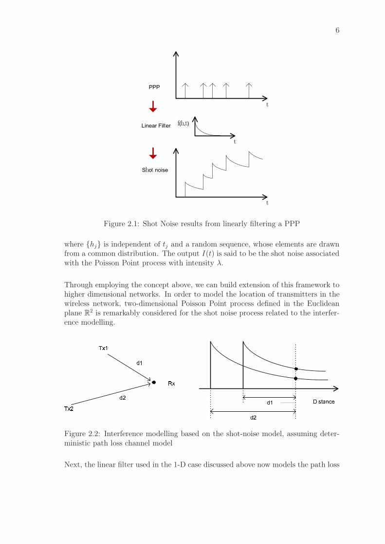
Through employing the concept above, we can build extension of this framework tohigher dimensional networks. In order to model the location of transmitters in thewireless network, two-dimensional Poisson Point process defined in the Euclideanplane R

2 is remarkably considered for the shot noise process related to the interfer-ence modelling.

Figure 2.2: Interference modelling based on the shot-noise model, assuming deter-ministic path loss channel model

Next, the linear filter used in the 1-D case discussed above now models the path loss

7

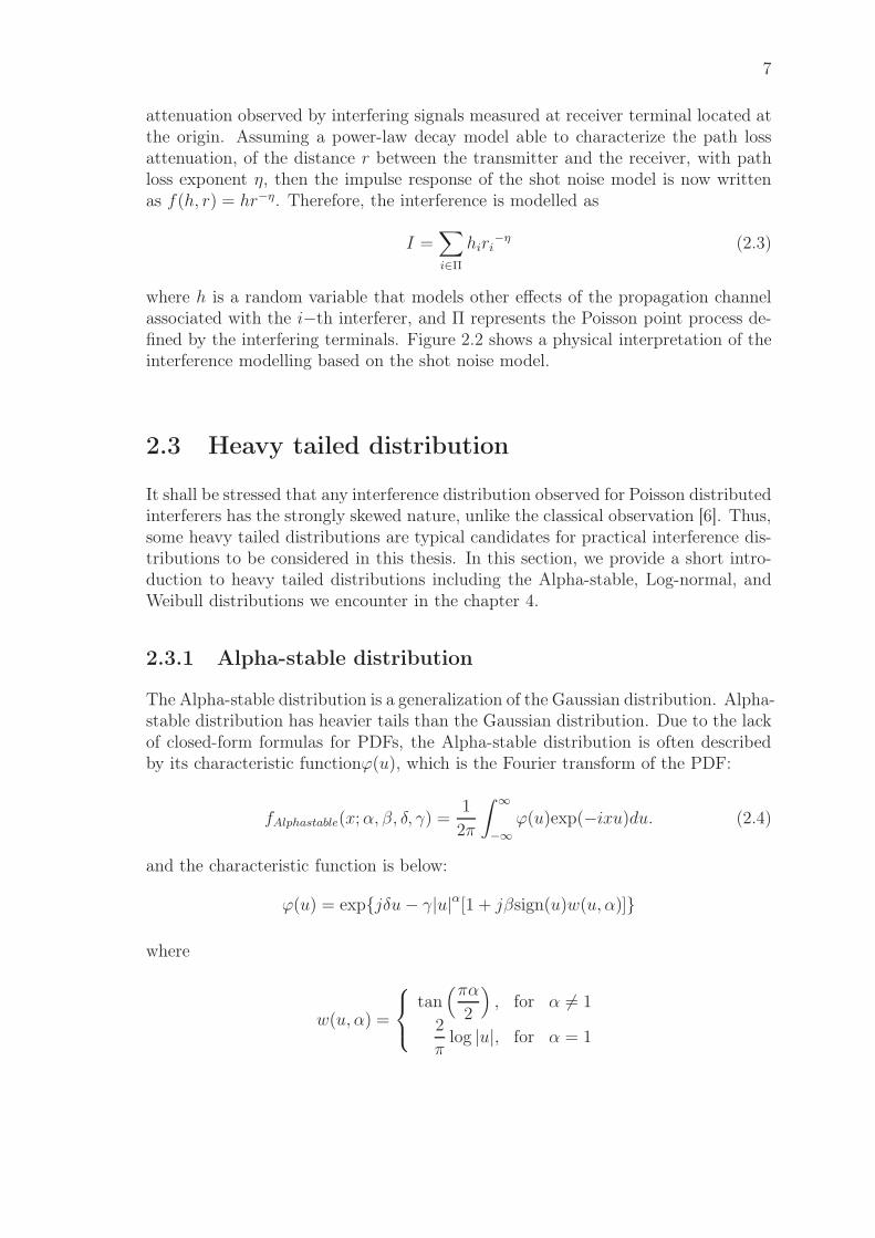
attenuation observed by interfering signals measured at receiver terminal located atthe origin. Assuming a power-law decay model able to characterize the path lossattenuation, of the distance r between the transmitter and the receiver, with pathloss exponent η, then the impulse response of the shot noise model is now writtenas f(h, r) = hr−η. Therefore, the interference is modelled as

I =∑

i∈Π

hiri−η (2.3)

where h is a random variable that models other effects of the propagation channelassociated with the i−th interferer, and Π represents the Poisson point process de-fined by the interfering terminals. Figure 2.2 shows a physical interpretation of theinterference modelling based on the shot noise model.

2.3 Heavy tailed distribution

It shall be stressed that any interference distribution observed for Poisson distributedinterferers has the strongly skewed nature, unlike the classical observation [6]. Thus,some heavy tailed distributions are typical candidates for practical interference dis-tributions to be considered in this thesis. In this section, we provide a short intro-duction to heavy tailed distributions including the Alpha-stable, Log-normal, andWeibull distributions we encounter in the chapter 4.

2.3.1 Alpha-stable distribution

The Alpha-stable distribution is a generalization of the Gaussian distribution. Alpha-stable distribution has heavier tails than the Gaussian distribution. Due to the lackof closed-form formulas for PDFs, the Alpha-stable distribution is often describedby its characteristic functionϕ(u), which is the Fourier transform of the PDF:

fAlphastable(x;α, β, δ, γ) =1

2π

∫

∞

−∞

ϕ(u)exp(−ixu)du. (2.4)

and the characteristic function is below:

ϕ(u) = exp{jδu− γ|u|α[1 + jβsign(u)w(u, α)]}

where

w(u, α) =

tan(πα

2

)

, for α 6= 1

2

πlog |u|, for α = 1

8

sign(u) =

1, for u > 00, for u = 0

−1, for u < 0

with the following definition for four parameters:

−5 0 50

0.1

0.2

0.3

0.4

0.5

0.6

= 0.5 = 0.75 = 1.0 = 1.25 = 1.5α

αααα

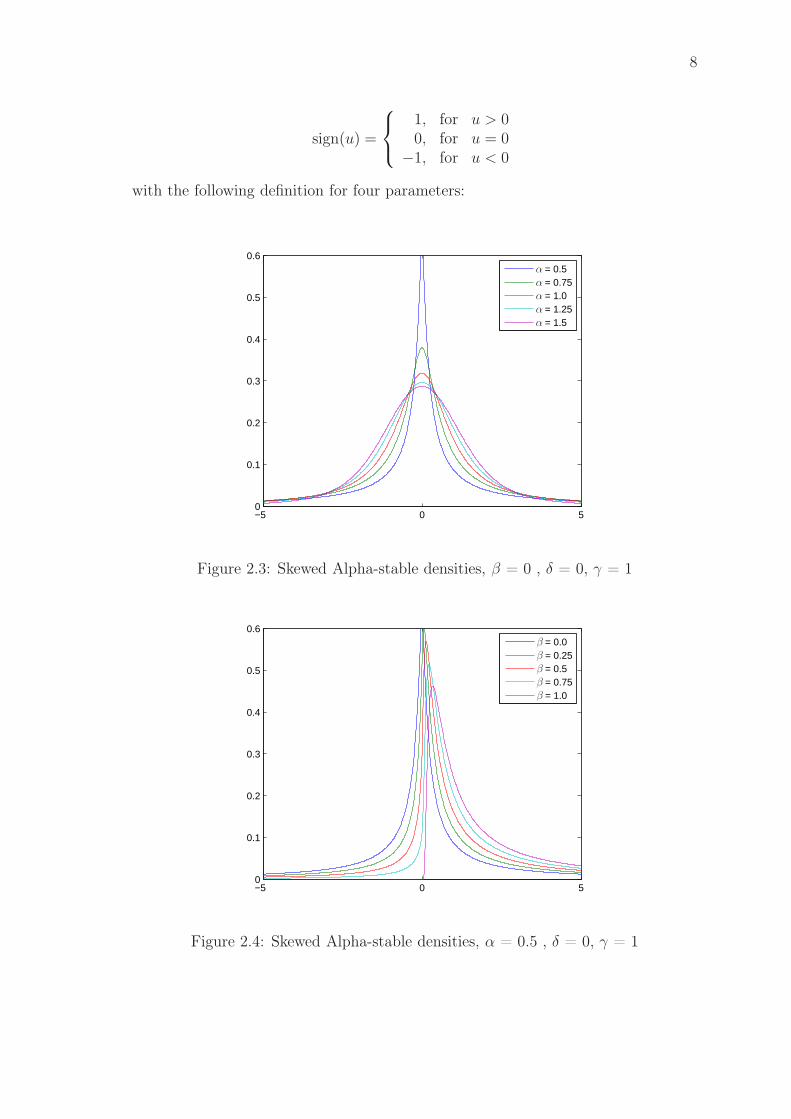
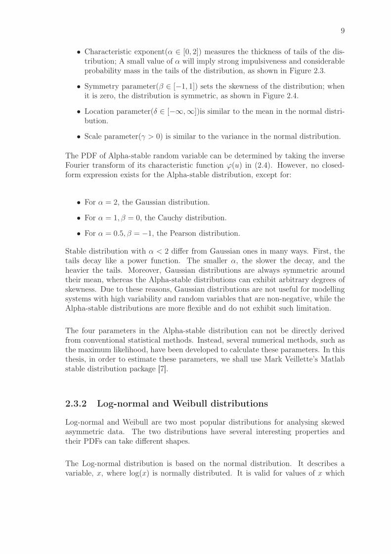
Figure 2.3: Skewed Alpha-stable densities, β = 0 , δ = 0, γ = 1

−5 0 50

0.1

0.2

0.3

0.4

0.5

0.6

= 0.0 = 0.25 = 0.5 = 0.75 = 1.0β

ββββ

Figure 2.4: Skewed Alpha-stable densities, α = 0.5 , δ = 0, γ = 1

9

• Characteristic exponent(α ∈ [0, 2]) measures the thickness of tails of the dis-tribution; A small value of α will imply strong impulsiveness and considerableprobability mass in the tails of the distribution, as shown in Figure 2.3.

• Symmetry parameter(β ∈ [−1, 1]) sets the skewness of the distribution; whenit is zero, the distribution is symmetric, as shown in Figure 2.4.

• Location parameter(δ ∈ [−∞,∞])is similar to the mean in the normal distri-bution.

• Scale parameter(γ > 0) is similar to the variance in the normal distribution.

The PDF of Alpha-stable random variable can be determined by taking the inverseFourier transform of its characteristic function ϕ(u) in (2.4). However, no closed-form expression exists for the Alpha-stable distribution, except for:

• For α = 2, the Gaussian distribution.

• For α = 1, β = 0, the Cauchy distribution.

• For α = 0.5, β = −1, the Pearson distribution.

Stable distribution with α < 2 differ from Gaussian ones in many ways. First, thetails decay like a power function. The smaller α, the slower the decay, and theheavier the tails. Moreover, Gaussian distributions are always symmetric aroundtheir mean, whereas the Alpha-stable distributions can exhibit arbitrary degrees ofskewness. Due to these reasons, Gaussian distributions are not useful for modellingsystems with high variability and random variables that are non-negative, while theAlpha-stable distributions are more flexible and do not exhibit such limitation.

The four parameters in the Alpha-stable distribution can not be directly derivedfrom conventional statistical methods. Instead, several numerical methods, such asthe maximum likelihood, have been developed to calculate these parameters. In thisthesis, in order to estimate these parameters, we shall use Mark Veillette’s Matlabstable distribution package [7].

2.3.2 Log-normal and Weibull distributions

Log-normal and Weibull are two most popular distributions for analysing skewedasymmetric data. The two distributions have several interesting properties andtheir PDFs can take different shapes.

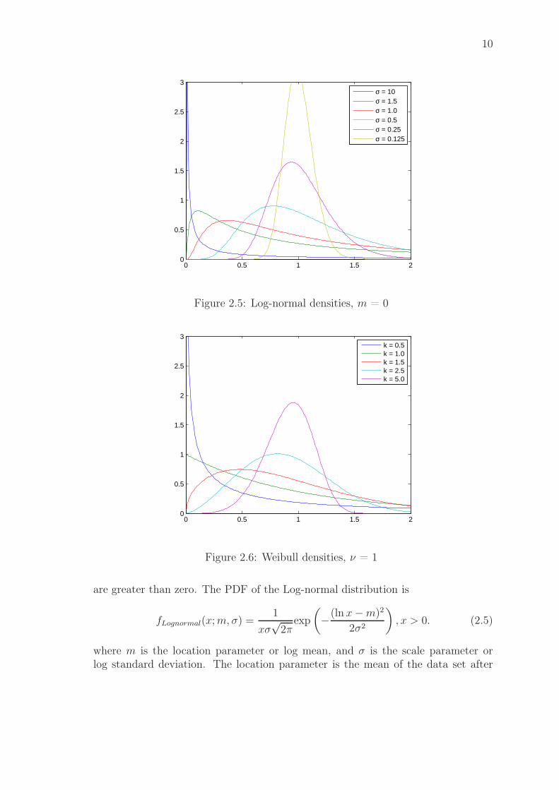
The Log-normal distribution is based on the normal distribution. It describes avariable, x, where log(x) is normally distributed. It is valid for values of x which

10

0 0.5 1 1.5 20

0.5

1

1.5

2

2.5

3

σ = 10σ = 1.5σ = 1.0σ = 0.5σ = 0.25σ = 0.125

Figure 2.5: Log-normal densities, m = 0

0 0.5 1 1.5 20

0.5

1

1.5

2

2.5

3

k = 0.5k = 1.0k = 1.5k = 2.5k = 5.0

Figure 2.6: Weibull densities, ν = 1

are greater than zero. The PDF of the Log-normal distribution is

fLognormal(x;m, σ) =1

xσ√2π

exp

(

−(ln x−m)2

2σ2

)

, x > 0. (2.5)

where m is the location parameter or log mean, and σ is the scale parameter orlog standard deviation. The location parameter is the mean of the data set after

11

transformation by taking the logarithm, and the scale parameter is the standarddeviation of the data set after transformation. The Log-normal distribution takeson several shapes depending on the value of the shape parameter. The Log-normaldistribution is skewed right, and the skewness increases as the value of σ increases.Similarly, the density function of a Weibull distribution, with scale parameter ν>0and shape parameter k>0 is

fWeibull(x; ν, k) = kν−kx(k−1)exp(

−x

ν

)k

, x > 0. (2.6)

In chapter 4, lognfit and wblfit functions included in Matlab Statistical Toolboxare used to estimate the parameters for the Log-normal and Weibull distributions.

Chapter 3

SYSTEM MODEL

In this chapter, we present the system model, and apply some of the techniques in-troduced in the previous section to study the interference in ad hoc networks. Thischapter is organized as follows: We begin with channel model and MAC model inSection 3.1 and 3.2 respectively. For interference model, Section 3.3 presents someresults on Laplace functional of Poisson shot noise processes. Some Interferencemodels for CSMA/CA network, that is, exclusively deployed nodes, are introducedand discussed in Section 3.4.

3.1 Propagation Channel Model

The two main propagation effects considered in this thesis are: (1) deterministicpath loss and (2) small scale fading. These effects are described in the following.

Deterministic path loss models the attenuation suffered by a signal while travelingfrom the transmitter to the receiver. At a given location x, the power of a signalreceived from node y is given by P l(x; y). P is the transmission power of node y,and a function l(x; y) gives the attenuation (path loss) from y to x in R

2. For thedeterministic path loss function, the following singular model will be our defaultassumption in this thesis. We will take for η > 2:

l(r) = l(x; y) = l(|x− y|) = 1

|x− y|η = r−η (3.1)

where η is the path loss exponent.

Propagation occurs through multiple paths between transmitter and receiver in atypical wireless communication environment, and several replicas of the transmittedsignal reaching the receive antenna can be considered as a spatially non correlatedand time variant process. These replicas combine with each other in a constructive ordestructive way, resulting in a received signal with rapid envelope fluctuation. Sev-

12

13

eral classical statistical distributions are commonly used to describe the envelope (orpower) of the received signal. In this thesis, the amplitude fading is assumed to bethe Rayleigh distribution. The functional form of the Rayleigh fading distribution is

Pr(a) =a

σ2exp

(−a2

2σ2

)

(3.2)

where a is the envelope amplitude of the received signal, and σ2 is the pre-detectionmean power of the multipath signal. When dealing with received signal powers, thepower fading variable is used by denoting P = a2, exploiting that the probabilitydensity function for the power is

Pr(P ) =1

P̄exp

(

−P

P̄

)

(3.3)

where P stands for power and P̄ is the mean of P , that is, the received signal powerby path loss which is exponentially distributed with unit mean.

3.2 Medium Access Control

IEEE 802.11 DCF is considered for the CSMA/CA protocols [25]. The mediumaccess control (MAC) protocol defines the rules for assessing the radio medium.The mechanism to determine whether or not the medium is busy is called CCA(Clear Channel Assessment). In this thesis, CCA is performed according to thefollowing mode:

• Energy above threshold. CCA shall report a busy medium upon detectionof accumulative signal power above a threshold called carrier sense threshold,ICSTh. In this case, it could be expressed as

∑

i Pil(ri) ≤ ICSTh where ri is thedistance from the effective node i to the sensing node, and the random partsof noise is not considered.

Given a carrier sense threshold, ICSth, the corresponding carrier sense range, DCS,is defined as the minimum distance allowed between two concurrent transmitters.In practical simulation by NS-2 which shall be introduced in next Chapter, CCAEnergy above threshold Mode above is performed so that aggregate interferencepower value is evaluated with a given ICSTh. In fact, DCS is a non-deterministicparameter that can significantly affect the MAC performance in ad hoc networks. Itbalances the trade-off between the amount of spatial frequency reuse and the likeli-hood of packet collision. Therefore, it should be carefully chosen, based on networkparameters such as network topology, traffic pattern, and transceiver power.

14

However, the deterministic carrier sense range is used e.g. in [9] [11] by exploitingthe one-to-one mapping between a ICSTh, and a DCS. There is a further attemptto find the optimum carrier sensing range to maximize the throughput in [10]. Forsimplicity, point processes which shall be introduced in this Chapter employ thedeterministic DCS which can be expressed as:

Dcs =

(

P0

ICSTh

)1/η

(3.4)

where P0 is transmission power and DCS is carrier sense range.

3.3 Interference Models for PPP spatial node dis-

tribution

Nodes are deployed randomly at positions specified by a Poisson distribution. Forthe space R

2, the probability that the area A in a PPP has n number of nodes is

Pr(N = n) =(λA)n

n!exp(−λA) (3.5)

where N is the number of points and λ is the intensity(also called density) measurefor the infinite planar. Then, we obtain the interference from nodes deployed by thePPP with node density λPPP which are the number of the potential and effectivetransmitters on the plane R

2. Node geometry for PPP with λPPP−eff follows:

ΦPPP = {(XiPPP , (ei

PPP , PiPPP ))}, (3.6)

where we have the following.

• {i} denotes a node’s index.

• {Xi} denotes the location of the node i.

• {ei} denotes the medium access indicator of the node i; ei=0 means that thenode is a potential receiver. ei=1 means that the node is a effective transmitter.The random variable ei are independent, with Pr(ei = 1) = peff . The effectivefactor peff is the probability that a node has a packet to be transmitted atsome time instant. Then we can express that λPPP−eff = λPPPpeff .

• {Pi} denotes the powers emitted by the station whose ei is 1; The randomvariable {Pi} are assumed to be independently and identically distributed withexponentially distributed powers with mean 1/µ.

15

Suppose that interference sensed at a node located at y ∈ R2 follows process ΦPPP .Through using the concept of shot noise process introduced in Chapter 2 and theattenuation function shown in Subsection 3.1, the shot noise process of ΦPPP canbe represented as

IΦPPP(y) =

∑

Xi∈ΦPPP

Pil(|y −Xi|). (3.7)

Except for the path loss η = 4 case, the closed form of the shot noise distributionis not known for the other values of the path loss. In [8], the mean total receivedpower is known as :

E[IΦPPP] = E[1/µ]λPPP−eff

∫

R2

l(|y|)dy =2πλPPP−eff

µ

∫

∞

0

rl(r)dr (3.8)

and the Laplace transform is also known as:

LIΦPPP(s) = exp

{

−2πλPPP−eff

∫

∞

0

r

1 + µ/(sl(r))dr

}

= exp

{

−λPPP−eff

(

s

µ

)(2/η)

K(η)

}

, (3.9)

where K(η) =2π2

η sin(2π/η)=

2πΓ(2/η)Γ(1− 2/η)

ηand Γ(z) =

∫

∞

0tz−1e−tdt is the

Gamma function.

For η = 4 case, the PDF and CDF exists. From Lf(s) = s · LF (s), CDF [28] [8] is:

FIΦPPP(t) = Pr(IΦPPP

≤ t)

= L−1

exp

{

−λPPP−eff

(

s

µ

)(1/2)

K(4)

}

s

= efrc

λPPP−effK(4)√µ

2√t

= efrc

(

λPPP−effπ2

4õt

)

(3.10)

by using the fact that inverse Laplace transform ofexp(−a

√s)

s, a ≥0, is erfc

(

a

2√t

)

,

where erfc(x) =2√π

∫

∞

xe−t2dt is a complementary error function. Accordingly, PDF

16

is:

fIΦPPP(t) =

d

dtFIΦPPP

(t)

=

exp

(

π4λPPP−eff2

16µt

)

π3/2µλPPP−eff

4(µt)3/2(3.11)

3.4 Interference Models for Exclusively Deployed

Nodes

According to CSMA/CA, only one can get a chance to access the channel amongmultiple nodes within overlapped carrier sensing region. Each node should be sur-vived or discarded according to whether the distance between the nearest effectivenodes is greater than the carrier sense range. In this thesis, only effective nodes areconsidered for interference models.

3.4.1 Poisson Point Process with modified density

In order to model the carrier sense range, the hard-core point process, in whichthe constituent points are forbidden to lie closer together than a certain minimumdistance, one of thinning functioned process of initial point process is used in [4].Thinning function means to discard certain existed points according to a given pol-icy. since the determination of surviving points depends on the relative distance toother points already determined to survive, this thinning has a dependent charac-teristic.

In this model, the eventual node geometry which we consider here follows:

ΦPPPmd = {(XiPPPmd, (ei

PPPmd, PiPPPmd))} (3.12)

with modified node density measure given as follows:

λPPPmd =1− exp(−λPPP−effπDCS

2)

πDCS2 (3.13)

where PPPmd denotes PPP with modified density. DCS is the carrier sensing range.Elements of this process are ei

PPPmd = 1 and PiPPPmd = Pi as in (3.6) respectively.

For CDF [28] [8] of the new shot noise interference in η = 4 case, we replace

17

λPPP−eff of (3.11) with this new node density, λPPPmd:

FIΦPPPmd(t) = erfc

(

λPPPmdπ2

4õt

)

(3.14)

Accordingly, PDF is

fIΦPPPmd(t) =

d

dtFIΦPPPmd

(t) =

exp

(−π4λPPPmd2

16µt

)

π3/2µλPPPmd

4(µt)3/2(3.15)

3.4.2 Matérn Point Process

An alternate temporal sequence version of the Matérn point process could be ad-vocated [1] [2] to model interference in CSMA/CA network. A process where asubset of transmitters has been already chosen, is needed for the measure of the in-terference at a given point. So, a temporal scheduling between the points is requred.

A temporal Matérn point process is defined as an iterative procedure that sequen-tially tries to place n non-overlapping discs of radius DCS in the plane. Denote thisprocess ΦMPP where MPP means Matérn Point Process. In this subsection, westart with this point process built as follows:

ΦMPP = {(XiMPP , (ei

MPP , PiMPP ))} (3.16)

Elements of this process are eiMPP = 1 and Pi

MPP = Pi as in (3.6) respectively.Then, ΦMPP is developed as follows:

• Let N be a positive integer.

• Let Xi, where i = 1, ..., N , be a sequence of random variables independentlyand uniformly distributed in finite observation, B(O,R), the ball of radius Rcentered at O.

• Let ΦMPP (i) be the set of points selected after i steps.

• At the ith step, the point Xi is distributed and selected in ΦMPP (i) if and onlyif none of the i − 1 previous points, even the inactive ones, lies in the finiteplane BXi

, the ball centered at Xi with radius DCS.

• After all of the N points are processed with discrete Poisson distribution, theprocedure finally ends.

• The point X1 is distributed first and systematically selected in ΦMPP (1).

18

• The Matérn point process ΦMPP (N) is built for i ∈ [2, N ] according to:

X(i) ∈ ΦMPP (i), iif |Xi −Xj| > DCS ∀j ∈ [1, i− 1] (3.17)

At each step, a new node attempts to access the channel medium. If its distanceto all other points is greater than the carrier sensing range, it succeeds. Otherwise,the node is kept inactive. However, this inactive node is involved in the selectionprocess of the following points. Note that the selection of a new point as activenode depends on all previous points, even the inactive ones. This illustrates a spa-tial anomaly of the Matérn process related to the fact that inactive nodes give animpact on the selection process. In the end, the fact that unselected nodes playa role in the selection process limits the node coverage to a portion of the plane.The consequence is an underestimation of the effective transmitters density in thenetwork and so far an underestimation of the interference.

3.4.3 Simple Sequential Inhibition

In order to complement the flaws of the alternate temporal sequence version of theMatérn point process presented in previous subsection, we discuss another point pro-cess, the Simple Sequential Inhibition(SSI) point process, which is first introducedby Palasti [12] and seems to be more appropriate model for CSMA/CA networks.

In this subsection, we start with the point process built as follows:

ΦSSI = {(XiSSI , (ei

SSI , PiSSI))} (3.18)

Elements of this process are eiSSI = 1 and Pi

SSI = Pi as in (3.6) respectively. Then,ΦSSI is developed as follows:

• Let N be a positive integer.

• Let Xi, where i = 1, ..., N , be a sequence of random variables independentlyand uniformly distributed in finite observation, B(O,R).

• Let ΦSSI(i) be the set of points selected after i steps.

• At the ith step, the point Xi is distributed and selected in ΦSSI(i) if and onlyif none of the i−1 previous points, only the active ones, lies in the finite planeBXi

, the ball centered at Xi with radius DCS.

• After all of the N points are processed with discrete Poisson distribution, theprocedure finally ends.

• The point X1 is distributed first and systematically selected in ΦSSI(1).

19

• The SSI point process ΦSSI(N) is built for i ∈ [2, N ] according to:

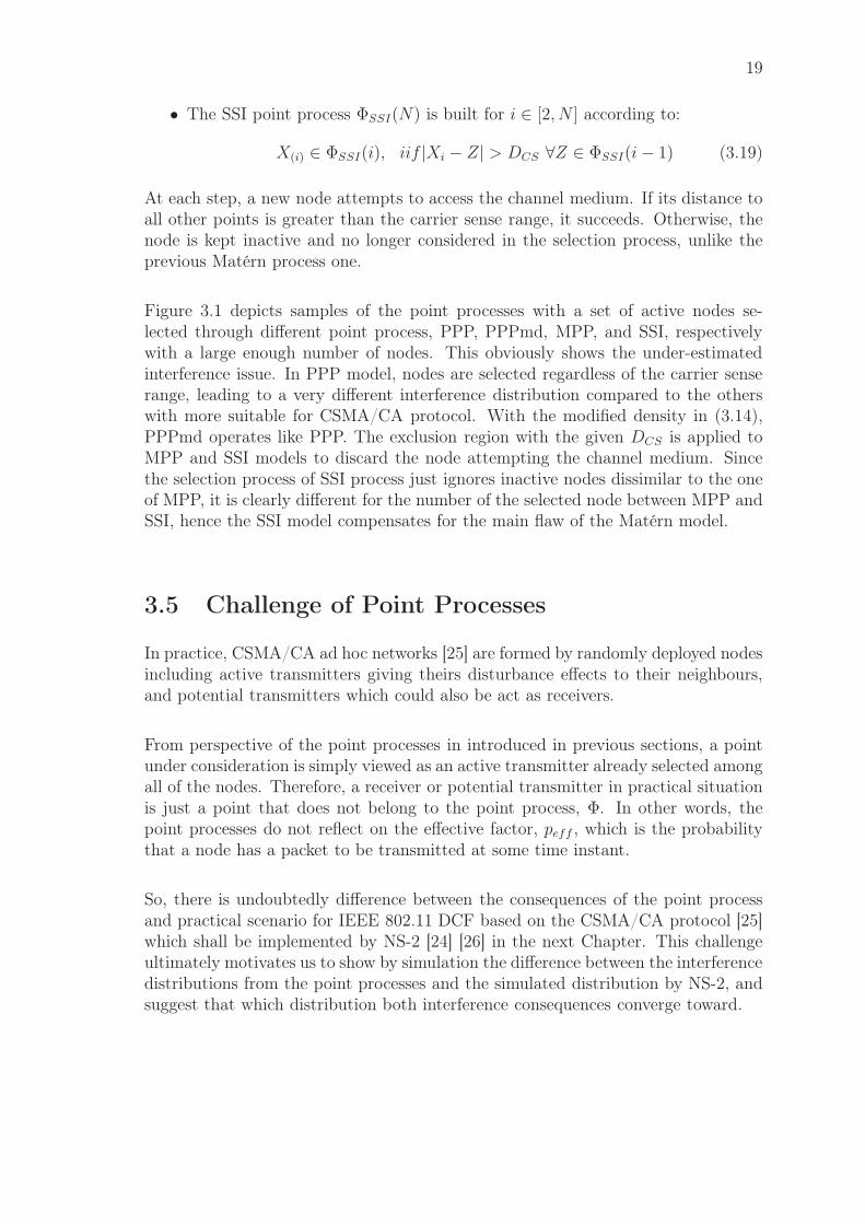
X(i) ∈ ΦSSI(i), iif |Xi − Z| > DCS ∀Z ∈ ΦSSI(i− 1) (3.19)

At each step, a new node attempts to access the channel medium. If its distance toall other points is greater than the carrier sense range, it succeeds. Otherwise, thenode is kept inactive and no longer considered in the selection process, unlike theprevious Matérn process one.

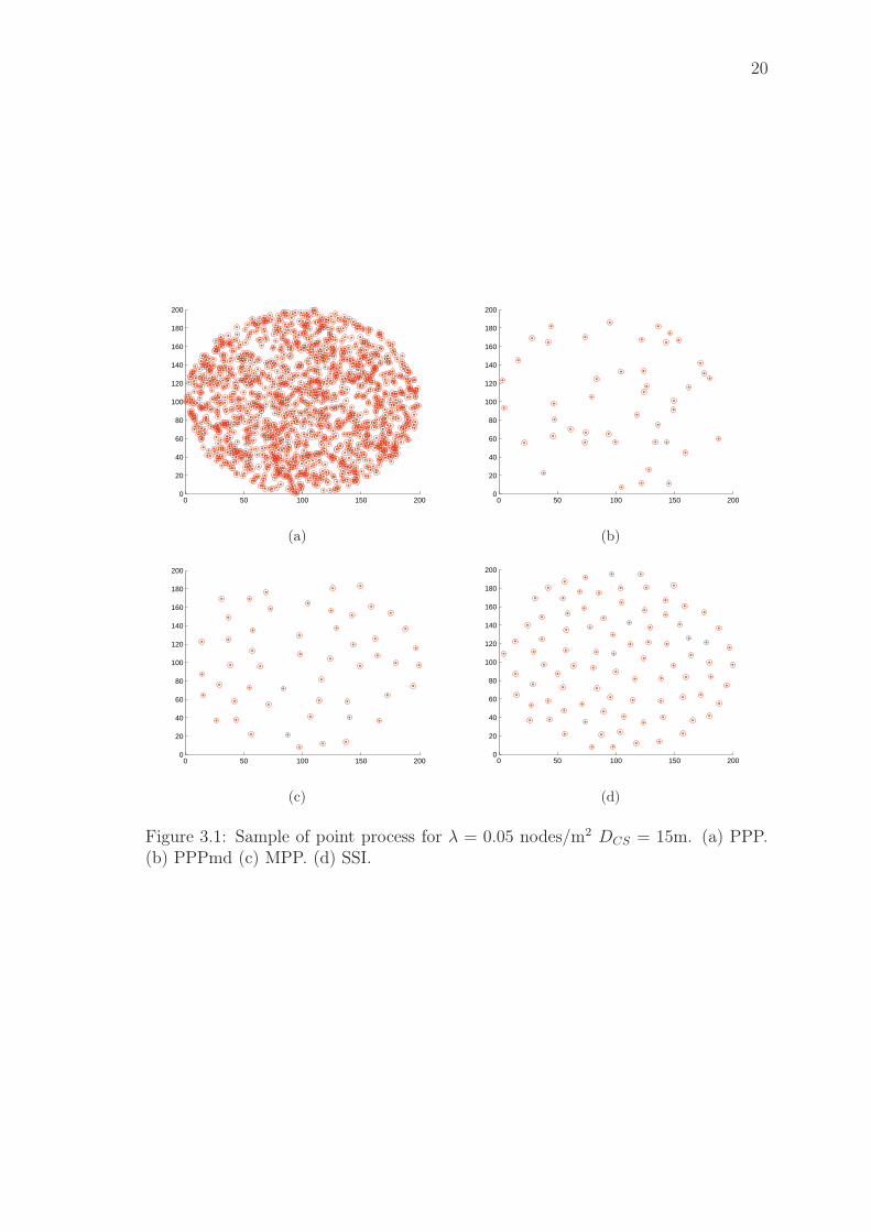
Figure 3.1 depicts samples of the point processes with a set of active nodes se-lected through different point process, PPP, PPPmd, MPP, and SSI, respectivelywith a large enough number of nodes. This obviously shows the under-estimatedinterference issue. In PPP model, nodes are selected regardless of the carrier senserange, leading to a very different interference distribution compared to the otherswith more suitable for CSMA/CA protocol. With the modified density in (3.14),PPPmd operates like PPP. The exclusion region with the given DCS is applied toMPP and SSI models to discard the node attempting the channel medium. Sincethe selection process of SSI process just ignores inactive nodes dissimilar to the oneof MPP, it is clearly different for the number of the selected node between MPP andSSI, hence the SSI model compensates for the main flaw of the Matérn model.

3.5 Challenge of Point Processes

In practice, CSMA/CA ad hoc networks [25] are formed by randomly deployed nodesincluding active transmitters giving theirs disturbance effects to their neighbours,and potential transmitters which could also be act as receivers.

From perspective of the point processes in introduced in previous sections, a pointunder consideration is simply viewed as an active transmitter already selected amongall of the nodes. Therefore, a receiver or potential transmitter in practical situationis just a point that does not belong to the point process, Φ. In other words, thepoint processes do not reflect on the effective factor, peff , which is the probabilitythat a node has a packet to be transmitted at some time instant.

So, there is undoubtedly difference between the consequences of the point processand practical scenario for IEEE 802.11 DCF based on the CSMA/CA protocol [25]which shall be implemented by NS-2 [24] [26] in the next Chapter. This challengeultimately motivates us to show by simulation the difference between the interferencedistributions from the point processes and the simulated distribution by NS-2, andsuggest that which distribution both interference consequences converge toward.

20

0 50 100 150 2000

20

40

60

80

100

120

140

160

180

200

(a)

0 50 100 150 2000

20

40

60

80

100

120

140

160

180

200

(b)

0 50 100 150 2000

20

40

60

80

100

120

140

160

180

200

(c)

0 50 100 150 2000

20

40

60

80

100

120

140

160

180

200

(d)

Figure 3.1: Sample of point process for λ = 0.05 nodes/m2 DCS = 15m. (a) PPP.(b) PPPmd (c) MPP. (d) SSI.

Chapter 4

Simulation Results and Analysis

The aim of this section is to validate how the practical results generated by NS-2simulator match the different point processes introduced in previous Chapter. Wethen perform hypothesis test to check whether the empirical interference distribu-tion could be extrapolated by some considered distribution. In Section 4.1, we firstbriefly show comparisons between the Matlab simulation results and the theoreticalclosed forms derived from PPP and PPP with modified density. On the basis ofthis certainty, we can extend our validation with NS-2 simulator. Simulation pa-rameters and scenario used in NS-2 are introduced in Section 4.2. We carry out thecomparison among the point processes in Section 4.3, and the existing gap betweeninterferences from different processes and NS-2 is discussed in Section 4.4. Hypoth-esis test is executed in Section 4.5.

4.1 NS-2 Simulation Set-up

The simulations have been performed using NS-2 [24]. It is discrete event simulatorand more common among researchers’ community since it is an open- source simu-lator. The NS-2.34 version, the latest version [24] [26], is used for our experiments.Since cumulative SINR computation is offered by continuously tracking the sum ofall reception power values of all frames arriving in parallel and of the noise floor,such significant information makes it possible to obtain the aggregate interferencepower level.

In simulator, PowerMonitorthreshold is used to reduce the number of entriesrecorded in the interference list. For example, if a signal power from a transmitteris less than the value of this PowerMonitorthreshold at a receiver, the receiverdoes not consider the transmitter as an interferer giving an effect on the aggre-gate interference power. In our simulation, we use a small enough value of thePowerMonitorthreshold value so that all of nodes in a grid can be monitored and

21

22

considered as interferers.

Preamblecapture feature is used in this simulation. While the receiver node is re-ceiving the preamble and PLCP(Physical Layer Convergence Procedure) header ofan earlier frame, if a new frame arrives at the receiver and it has sufficiently higherpower which is PreambleCaptureThreshold value above the earlier one, the newframe can be picked. Likewise, while the receiver node is receiving the data of anearlier frame, if a new frame arrives at the receiver and it has sufficiently higherpower which is DataCaptureThreshold value above the earlier one, then it immedi-ately abandons the previous frame and attempts to decode the preamble and PLCPheader of the new frame.

MAC header is transmitted with defined BPSK modulation(6Mbps), while the MACdata can be coded in a much higher modulation scheme, but in our simulation, it isalso coded with BPSK modulation.

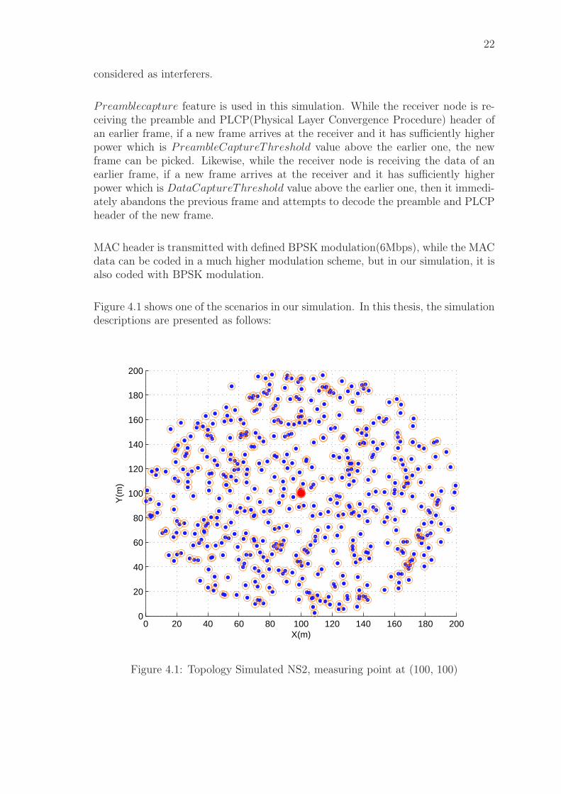
Figure 4.1 shows one of the scenarios in our simulation. In this thesis, the simulationdescriptions are presented as follows:

0 20 40 60 80 100 120 140 160 180 2000

20

40

60

80

100

120

140

160

180

200

X(m)

Y(m

)

Figure 4.1: Topology Simulated NS2, measuring point at (100, 100)

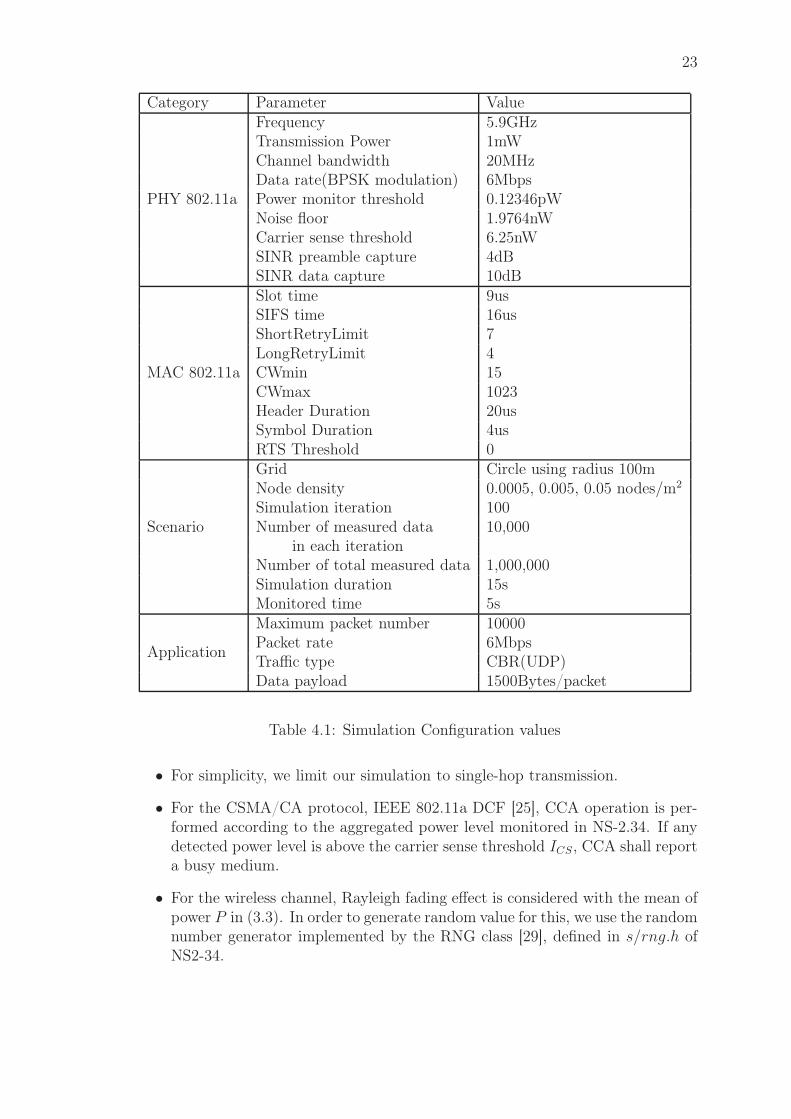
23

Category Parameter Value

PHY 802.11a

Frequency 5.9GHzTransmission Power 1mWChannel bandwidth 20MHzData rate(BPSK modulation) 6MbpsPower monitor threshold 0.12346pWNoise floor 1.9764nWCarrier sense threshold 6.25nWSINR preamble capture 4dBSINR data capture 10dB

MAC 802.11a

Slot time 9usSIFS time 16usShortRetryLimit 7LongRetryLimit 4CWmin 15CWmax 1023Header Duration 20usSymbol Duration 4usRTS Threshold 0

Scenario

Grid Circle using radius 100mNode density 0.0005, 0.005, 0.05 nodes/m2

Simulation iteration 100Number of measured data 10,000

in each iterationNumber of total measured data 1,000,000Simulation duration 15sMonitored time 5s

Application

Maximum packet number 10000Packet rate 6MbpsTraffic type CBR(UDP)Data payload 1500Bytes/packet

Table 4.1: Simulation Configuration values

• For simplicity, we limit our simulation to single-hop transmission.

• For the CSMA/CA protocol, IEEE 802.11a DCF [25], CCA operation is per-formed according to the aggregated power level monitored in NS-2.34. If anydetected power level is above the carrier sense threshold ICS, CCA shall reporta busy medium.

• For the wireless channel, Rayleigh fading effect is considered with the mean ofpower P in (3.3). In order to generate random value for this, we use the randomnumber generator implemented by the RNG class [29], defined in s/rng.h ofNS2-34.

24

• By putting 0 into the value of RTS threshold, the RTS/CTS handshake isautomatically operated regardless of packet size which is 1500 Bytes withCBR in this thesis. The sending channel rate of the source node and packetrate are 6 Mbps, thereby making the traffic saturated.

• Wireless nodes are uniformly distributed in area of circle with radius R 100m."Uniformly distributed" means that all regions of the shape are equally likelyto be selected by the random number generator. More formally, the probabilityof a number falling in a particular region is proportional only to the area ofthe region. For this, let a node on a circle with R centered at origin be definedby (r cos(θ), r sin(θ)) where r is the distance [0, R] from the origin and θ is theangle [0, 2π]. The values of r and θ are generated by uniform function in theRNG class [29]. This implementation is illustrated in Appendix B.

• Transmission procedures are operated amongst themselves according to ran-domly generated traffic scenario which is presented in Appendix B. All of thegenerated nodes are assigned to start transmission to each destination at arandom time between 0 and 1 second until the maximum number 10000 ofpackets is transmitted or the simulation time 15 second is ended.

• The monitoring node (Red point in Figure 4.1) is additionally fixed at (100,100)to simply measure the aggregate power level of concurrent signals resultingfrom other nodes’ transmissions. The measuring operations occur at "Drop"event [26]. In perspective of this monitoring node, all of the concurrentlytransmitting packets are seen as interference signals, since no node transmitsa packet to the monitoring node as the transmitter’s destination in our simu-lation.

• The whole simulation runs 100 times, but for each iteration, we extract theinterference power level information within the specific time duration in orderto ensure the case all of the nodes start to participate into the transmission.

• For satisfying node distribution with a given node density, λ, at each iteration,the number of nodes in the area of a circle with radius R is generated as arandom variable with poisson distribution (3.5) with parameter λπR2 at eachiteration. The implemented code is shown in Appendix B.

• We sample 100,000 data from the measured total data, 1,000,000, from NS-2simulation,. Half of this sampled data is used for plotting the PDF or CDFdistributions of NS-2 result, and the other half is used for estimating theparameters of a considered distribution which shall encounter later as a fittingprocess.

Parameters used in our simulation are summarized in Table 4.1 with scenario de-scriptions. All the simulations presented later follow these parameters.

25

4.2 Theoretical and Experimental values of Inter-

ference distribution

As discussed in previous Chapter, the exact closed forms of the shot noise distribu-tion for PPP and PPPmd can be only obtained, when the path loss η is 4. Usingthe inverse Laplace transform technique, we can derive the CDFs and PDFs from(3.11), (3.12), (3.15), and (3.16). In this Section, we compare the values from thetheoretical closed form distribution with experimental results generated by Matlab,thereby providing the reliable foundation to compare with the practical ones basedon NS-2 in the following Section.

0

0.1

0.2

0.3

0.4

0.5

0.6

0.7

0.8

0.9

1

PPP(theo)

PPP(sim)

PPPmd(theo)

PPPmd(sim ceil)

PPPmd(sim floor)

Interference Power(dBm) on Log Scale

Cum

ula

tive

Dis

trib

uti

onFunct

ion

-80 -70 -60 -50 -40 -30 -20

(a)

0

0.005

0.01

0.015

0.02

0.025

0.03

PPP(theo)PPP(sim)PPPmd(theo)PPPmd(sim ceil)PPPmd(sim floor)

Interference Power(dBm) on Normal Scale

Pro

bab

ility

Den

sity

Funct

ion

-56.99 -52.22 -50.00 -48.54 -47.45

(b)

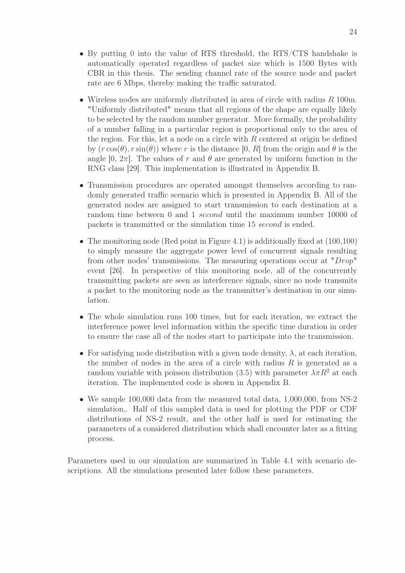
Figure 4.2: Theoretical results, and Experimental results in Matlab for λPPP =0.0005 nodes/m2 and λPPPmd = 0.0375 nodes/m2 when ICSTh= 6.25 nW. (a) CDF.(b) PDF.

In Figure 4.2, we have plotted the PDFs and CDFs of the interference. For simplic-ity, theo denotes the results from the closed forms, and sim denotes the simulationresults from Matlab.

When it comes to PPPmd, we consider the modified node density measure givenin (3.14) with the carrier sense range, DCS. In order to obtain the real integervalue from the modified node density, the number of nodes which is used in Matlabsimulation, we use the ceiling(⌈⌉) and floor(⌊⌋) functions. We note that the theoret-ical result for PPPmd is very close to the experimental results using the respectivenumber of nodes obtained by the ceiling and floor functions. Theoretical result andexperimental one for PPP are also seen to be same. Since the obtained densityby ceiling fucntion offers slightly more accurate result with theoretical one, we usethe result from node density using ceiling function for PPPmd from the next Section.

26

4.3 Process Comparisons

In this Section, we compare PDFs and CDFs of interferences of the 4 point processmodels, PPP, PPPmd, MPP and SSI, and NS-2 simulation. The interference distri-butions for different node densities are shown as well.

0

0.1

0.2

0.3

0.4

0.5

0.6

0.7

0.8

0.9

1

Cum

ula

tive

Dis

trib

uti

onFunct

ion

Interference Power(dBm) on Log Scale

PPPPPPmdMPPSSI

-70 -50 -30 -10 10

(a)

0

0.1

0.2

0.3

0.4

0.5

0.6

0.7

0.8

0.9

1

Cum

ula

tive

Dis

trib

uti

onFunct

ion

Interference Power(dBm) on Log Scale

PPPPPPmdMPPSSI

-70 -50 -30 -10 10

(b)

0

0.1

0.2

0.3

0.4

0.5

0.6

0.7

0.8

0.9

1

Cum

ula

tive

Dis

trib

uti

onFunct

ion

Interference Power(dBm) on Log Scale

PPPPPPmdMPPSSI

-70 -50 -30 -10 10

(c)

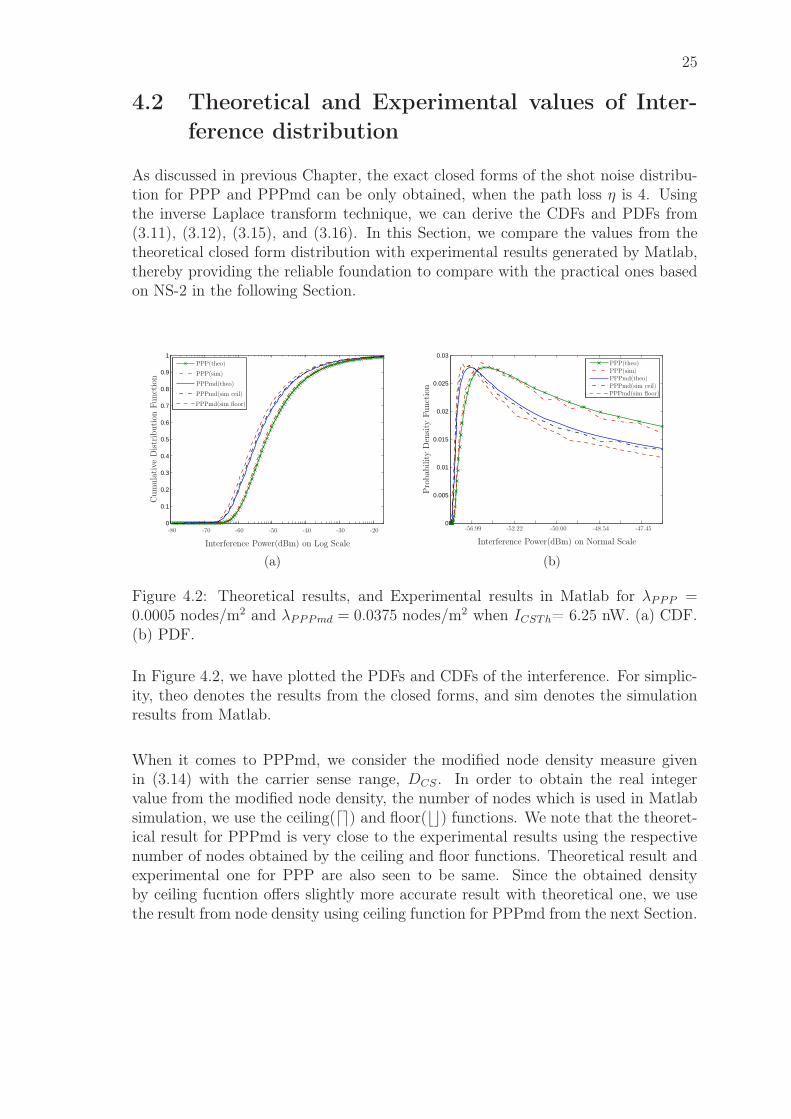
Figure 4.3: CDFs for the interference distributions of different processes, whenICSTh= 6.25 nW. (a) λ = 0.0005 nodes/m2. (b) λ = 0.005 nodes/m2, (c) λ = 0.05nodes/m2.

In Figures 4.3 (a) to (c), we compare the interference CDFs along with densityvariation for the point processes. For low λ, all of the point processes offer sim-ilar interference distributions one another. More precisely and analytically, theyall tend to follow the distribution of poisson point process. Since the possibilitythat some nodes reside within the radius, DCS of one node is relatively very low,thereby making CSMA/CA scheme considering any dependency between the differ-ent transmission location appears to operate independently like Aloha scheme. Asnode density gets larger, interference distributions among different point processesstart to differ more and more. For highest λ, the interference distribution by PPP

27

0

0.005

0.01

0.015

0.02

0.025

0.03

0.035

0.04

Pro

bab

ility

Den

sity

Funct

ion

Interference Power(dBm) on Normal Scale

PPPPPPmdMPPSSI

-50.00 -43.98 -41.55 -40.00

(a)

0

0.005

0.01

0.015

0.02

0.025

0.03

0.035

0.04

Pro

bab

ility

Den

sity

Funct

ion

Interference Power(dBm) on Normal Scale

PPPPPPmdMPPSSI

-50.00 -43.98 -41.55 -40.00

(b)

0

0.005

0.01

0.015

0.02

0.025

0.03

0.035

0.04

Pro

bab

ility

Den

sity

Funct

ion

Interference Power(dBm) on Normal Scale

PPPPPPmdMPPSSI

-50.00 -43.98 -41.55 -40.00

(c)

Figure 4.4: PDFs for the interference distributions of different processes, whenICSTh= 6.25 nW. (a) λ = 0.0005 nodes/m2. (b) λ = 0.005 nodes/m2, (c) λ = 0.05nodes/m2.

becomes far from the other point processes, since it still consider all of the effectivenodes unlike other processes.

In Figures 4.4 (a) to (c), the interference PDFs are plotted on a normal scale. Herewe can see that PDF’s peak point for each process is affected by a variation of den-sity. For very sparse network, all of the processes offer similar shapes one another. Indenser case, among the different point processes, there is huge dissimilarity regard-ing the variance of the distribution as well as peak point difference. Especially thedifference of MPP and SSI interference distributions get large in more dense case,resulting from the phenomenon in which SSI makes an effort to resolve the flaw ofMPP which underestimates the number of concurrent transmitters as discussed inprevious chapter. Accordingly, the interference value of SSI’s peak point is largerthan of MPP’s peak point.

Through Figure 4.5 summarily showing the interference distribution by NS-2, we

28

0

0.1

0.2

0.3

0.4

0.5

0.6

0.7

0.8

0.9

1

λ=0.0005

λ=0.005

λ=0.05

Cum

ula

tive

Dis

trib

uti

onFunct

ion

Interference Power(dBm) on Log Scale

-100 -90 -80 -70 -60 -50 -40 -30

(a)

0

0.005

0.01

0.015

0.02

0.025

0.03

λ=0.0005λ=0.005λ=0.05

Pro

bab

ility

Den

sity

Funct

ion

Interference Power(dBm) on Normal Scale

-70.00 -63.98 -61.55 -60.00

(b)

Figure 4.5: NS-2 simulation-based interference distribution for different values of λ,when ICSTh= 6.25 nW. (a) CDF. (b) PDF.

can confirm that the practical interference distribution also varies with the differentdensity.

4.4 Difference with NS-2 results

In Figure 4.6, the practical result by NS-2 and interference distributions by the pointprocesses are illustrated. Note that the interference distributions generated by thevarious point processes are significantly different with the practical results by NS-2.The main reason for the existence of gap is that node densities used in the inter-

29

0

0.1

0.2

0.3

0.4

0.5

0.6

0.7

0.8

0.9

1

Cum

ula

tive

Dis

trib

uti

onFunct

ion

Interference Power(dBm) on Log Scale

NS2PPPPPPmdMPPSSI

-90 -70 -50 -30 -10 10 30

(a)

0

0.1

0.2

0.3

0.4

0.5

0.6

0.7

0.8

0.9

1

Cum

ula

tive

Dis

trib

uti

onFunct

ion

Interference Power(dBm) on Log Scale

NS2PPPPPPmdMPPSSI

-90 -70 -50 -30 -10 10 30

(b)

0

0.1

0.2

0.3

0.4

0.5

0.6

0.7

0.8

0.9

1

Cum

ula

tive

Dis

trib

uti

onFunct

ion

Interference Power(dBm) on Log Scale

NS2PPPPPPmdMPPSSI

-90 -70 -50 -30 -10 10 30

(c)

Figure 4.6: Gap between NS-2 simulation-based interference distribution and Pointprocesses-based interference distributions, when ICSTh= 6.25 nW. (a) λ = 0.0005nodes/m2. (b) λ = 0.005 nodes/m2, (c) λ = 0.05 nodes/m2.

ference models are assumed to be effective node density representing only effectivetransmitters, not potential ones. Thus, the point process models simply concernthe aggregated interference power level which decays with distance from interferes,whereas the NS-2 simulation result is derived by nodes’ effective characteristic fac-tor, peff which practically results from some parameters related to MAC layer andApplication layer, such as initial contention window size, contention window size,retry-limit, traffic generation rate, and so on. Furthermore, different from the factthat the deterministic DCS is employed by (3.4) in the presented point process mod-els, DCS is nondeterministic in NS-2 simulation. Thus, DCS could be decided by theCCA mode(Energy above threshold) mentioned in Section 3.2 with a carrier sensethreshold ICSTh.

Nevertheless, since they all offer the similar shape: a peak and an asymmetry witha more or less heavy tail depending on the point process in Figure 4.7, it is enoughworth of notice. This observation absolutely contradicts a classical assumption in

30

0

0.005

0.01

0.015

0.02

0.025

0.03

0.035

0.04

Pro

bab

ility

Den

sity

Funct

ion

Interference Power(dBm) on Normal Scale

NS2PPPPPPmdMPPSSI

-50.00 -43.98 -41.55 -40.00

(a)

0

0.005

0.01

0.015

0.02

0.025

0.03

0.035

0.04

Pro

bab

ility

Den

sity

Funct

ion

Interference Power(dBm) on Normal Scale

NS2PPPPPPmdMPPSSI

-40.00 -33.98 -31.55 -30.00

(b)

0

0.005

0.01

0.015

0.02

0.025

0.03

0.035

0.04

Pro

bab

ility

Den

sity

Funct

ion

Interference Power(dBm) on Normal Scale

NS2PPPPPPmdMPPSSI

-40.00 -33.98 -31.55 -30.00

(c)

Figure 4.7: PDF shapes with asymmetric and heavy tailed behaviour, when ICSTh=6.25 nW. (a) λ = 0.0005 nodes/m2. (b) λ = 0.005 nodes/m2. (c) λ = 0.05 nodes/m2.

the signal processing community where the interference is generally considered to beGaussian [6]. Some researcher in [30] indicates that when considering the aggregateinterference, as a number of interferers in a network goes to infinity, the Gaussiandistribution is a proper approximation for the distribution of the aggregate inter-ference. However, we should pay attention to the fact that in the case where someof the interferers are dominant, the central limit theorem(CLT) [23] is not validanymore [31], even if the number of interferers may be large.

Figure 4.8 shows the PDFs of the interference distribution by NS-2, compared witha Gaussian distribution on Log Scale. Here, using normfit function in MATLABtoolbox, we fit the Gaussian distribution to the NS-2 result. According to Figure4.8 (a), there is obvious difference between the NS-2 result and Gaussian distribu-tion. Figure 4.8 (b) also shows that the distribution forming tail part of the overalldistribution is also hugely different from a Gaussian distribution, due to the heavytailed characteristic of the NS-2 result, which is mainly produced by the dominantinterferers around a node. In fact, different from other literatures [32] [33], in our

31

0

0.005

0.01

0.015

0.02

0.025

0.03

Gaussian

Pro

bab

ility

Den

sity

Funct

ion

Interference Power(dBm) on Log Scale

NS2

-70 -50 -30 -10

(a)

0

0.01

0.02

0.03

0.04

0.05

0.06

Gaussian

Pro

bab

ility

Den

sity

Funct

ion

Interference Power(dBm) on Log Scale

NS2

-50 -30 -10

(b)

0

0.01

0.02

0.03

0.04

0.05

0.06

Gaussian

Pro

bab

ility

Den

sity

Funct

ion

Interference Power(dBm) on Log Scale

NS2

-120 -110 -100 -90 -80 -70

(c)

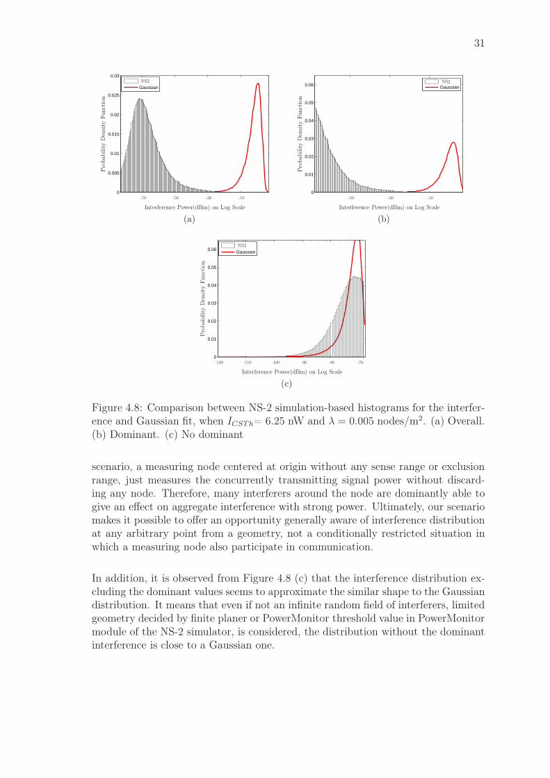
Figure 4.8: Comparison between NS-2 simulation-based histograms for the interfer-ence and Gaussian fit, when ICSTh= 6.25 nW and λ = 0.005 nodes/m2. (a) Overall.(b) Dominant. (c) No dominant

scenario, a measuring node centered at origin without any sense range or exclusionrange, just measures the concurrently transmitting signal power without discard-ing any node. Therefore, many interferers around the node are dominantly able togive an effect on aggregate interference with strong power. Ultimately, our scenariomakes it possible to offer an opportunity generally aware of interference distributionat any arbitrary point from a geometry, not a conditionally restricted situation inwhich a measuring node also participate in communication.

In addition, it is observed from Figure 4.8 (c) that the interference distribution ex-cluding the dominant values seems to approximate the similar shape to the Gaussiandistribution. It means that even if not an infinite random field of interferers, limitedgeometry decided by finite planer or PowerMonitor threshold value in PowerMonitormodule of the NS-2 simulator, is considered, the distribution without the dominantinterference is close to a Gaussian one.

32

4.5 Statistical Significance Test

In this section, the difference between point process models and NS-2 result is ob-jectively proven by value of statistics which simply offer the trend in variation ofnode density. We test several hypotheses that the interference by NS-2 conforms log-normal, Weibull or Alpha-stable distribution, and further obtain log-probabilities tofind the most similar distribution to the empirical one.

4.5.1 Hypothesis Checking Technique

We use the Matlab numeric computing environment and its Statistics Toolbox, acollection of tools supporting general statistical functions to curve fitting. Thetechniques of hypothesis checking consist of two basic procedures. First, values ofdistribution parameters are to be estimated by analysing experimental sample. Sec-ond, the null hypothesis that experimental data have a particular distribution withcertain parameters should be checked. To perform hypothesis checking itself, thekstest2 and chi2gof functions are used in the subsection 4.5.2 and 4.5.3, respec-tively or both.

4.5.2 process comparison with NS2 result

In this subsection, the kstest2 function, h = kstest2(x1,x2), performs a two-sampleKolmogorov-Smirnov test to compare the distributions of the values in the two datavectors, x1 and x2 which are interference results by NS-2 and one of the pointprocesses. The null hypothesis is that two vectors are from the same continuousdistribution. The alternative hypothesis is that they are from different continuousdistributions. Result h is equal to "1" if the hypothesis can be rejected, or "0" ifwe cannot reject that hypothesis. The function also returns the p-value which isthe probability that the null hypothesis can not be contradicted. The test statisticvalue is used to decide whether or not the null hypothesis should be rejected. In ourwork, we reject the hypothesis if the test is significant at the 5% level(p-value lessthan 0.05).

Let the first sample be the NS2 results with CDF F (x1) and squentially put oneof the different point processes into the second sample group with CDF Gi(x2), inorder to compare NS2 result with one of the processes.

H0 : F = Gi vs. H1 : F 6= Gi, ∀ i ∈ PointProcesses.

The statistic, shown in Table 4.2, is used to compare the fitness of NS-2 with eachprocess. For large sample size, the approximate critical value Dα is 0.0086 withα = 0.05 and n= 50000, according to this equation:

33

λ (nodes/m2) 0.0005 0.005 0.05

Critical Value (Dα) 8.601395e-03 8.601395e-03 8.601395e-03G1 PPPmd 7.981769e-01 8.225285e-01 7.368599e-01G2 MPP 8.105696e-01 8.605087e-01 7.908243e-01G3 SSI 8.124147e-01 9.110835e-01 9.021974e-01G4 PPP 8.391473e-01 9.640765e-01 9.931161e-01

Table 4.2: Kolmogorov-Smirnov test statistic for different density, when ICSTh= 6.25nW

Dα = c(α)

√

n1 + n2

n1n2

where n1 and n2 are the sample sizes of x1 and x2, respectively, and the coefficientc(α) is given by the table below.

α 0.10 0.05 0.025 0.01 0.005 0.001c(α) 1.22 1.36 1.48 1.63 1.73 1.95

Table 4.3: the coefficient c(α) values for α in [22]

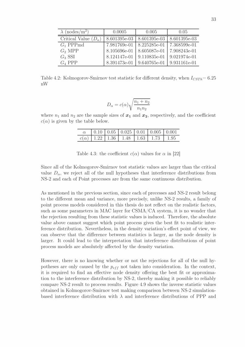
Since all of the Kolmogorov-Smirnov test statistic values are larger than the criticalvalue Dα, we reject all of the null hypotheses that interference distributions fromNS-2 and each of Point processes are from the same continuous distribution.

As mentioned in the previous section, since each of precesses and NS-2 result belongto the different mean and variance, more precisely, unlike NS-2 results, a family ofpoint process models considered in this thesis do not reflect on the realistic factors,such as some parameters in MAC layer for CSMA/CA system, it is no wonder thatthe rejection resulting from these statistic values is induced. Therefore, the absolutevalue above cannot suggest which point process gives the best fit to realistic inter-ference distribution. Nevertheless, in the density variation’s effect point of view, wecan observe that the difference between statistics is larger, as the node density islarger. It could lead to the interpretation that interference distributions of pointprocess models are absolutely affected by the density variation.

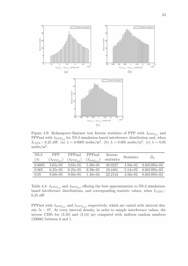
However, there is no knowing whether or not the rejections for all of the null hy-potheses are only caused by the peff not taken into consideration. In the context,it is required to find an effective node density offering the best fit or approxima-tion to the interference distribution by NS-2, thereby making it possible to reliablycompare NS-2 result to process results. Figure 4.9 shows the inverse statistic valuesobtained in Kolmogorov-Smirnov test making comparison between NS-2 simulation-based interference distribution with λ and interference distributions of PPP and

34

2 2.5 3 3.5 4 4.5 5

x 10−5

0

5

10

15

20

25

Inverse statistic

Inve

rse

stat

isti

c

λPPPeff, λPPPmd

nodes/m2

(a)

0.8 0.85 0.9 0.95 1 1.05 1.1 1.15 1.2

x 10−4

0

5

10

15

20

25

Inverse statistic

Inve

rse

stat

isti

c

λPPPeff, λPPPmd

nodes/m2

(b)

0.8 0.85 0.9 0.95 1 1.05 1.1 1.15 1.2

x 10−4

0

5

10

15

20

25

Inverse statistic

Inve

rse

stat

isti

c

λPPPeff, λPPPmd

nodes/m2

(c)

Figure 4.9: Kolmogorov-Smirnov test Inverse statistics of PPP with λPPPeffand

PPPmd with λPPPmdfor NS-2 simulation-based interference distribution and, when

ICSTh= 6.25 nW. (a) λ = 0.0005 nodes/m2. (b) λ = 0.005 nodes/m2. (c) λ = 0.05nodes/m2.

NS-2 PPP PPPmd PPPmd InverseStatistics Dα(λ) (λPPPeff

) (λPPPmd) (λ′

PPPeff) -statistics

0.0005 3.65e-05 3.65e-05 5.39e-05 20.0227 4.94e-02 8.601395e-030.005 6.25e-05 6.25e-05 9.39e-05 19.4401 5.14e-02 8.601395e-030.05 9.60e-05 9.60e-05 1.48e-04 22.2124 4.50e-02 8.601395e-03

Table 4.4: λPPPeffand λPPPmd

offering the best approximation to NS-2 simulation-based interference distributions, and corresponding statistic values, when ICSTh=6.25 nW

PPPmd with λPPPeffand λPPPmd

, respectively, which are varied with interval den-sity 5e − 07. At every interval density, in order to sample interference values, theinverse CDFs for (3.10) and (3.14) are computed with uniform random numbers(50000) between 0 and 1.

35

0

0.1

0.2

0.3

0.4

0.5

0.6

0.7

0.8

0.9

1

Cum

ula

tive

Dis

trib

uti

onFunct

ion

Interference Power(dBm) on Log Scale

NS2(λ)PPP(λPPPeff

),PPPmd(λPPPmd)

-110 -90 -70 -50 -30 -10

(a)

0

0.1

0.2

0.3

0.4

0.5

0.6

0.7

0.8

0.9

1

Cum

ula

tive

Dis

trib

uti

onFunct

ion

Interference Power(dBm) on Log Scale

NS2(λ)PPP(λPPPeff

),PPPmd(λPPPmd)

-110 -90 -70 -50 -30 -10

(b)

0

0.1

0.2

0.3

0.4

0.5

0.6

0.7

0.8

0.9

1

Cum

ula

tive

Dis

trib

uti

onFunct

ion

Interference Power(dBm) on Log Scale

NS2(λ)PPP(λPPPeff

),PPPmd(λPPPmd)

-110 -90 -70 -50 -30 -10

(c)

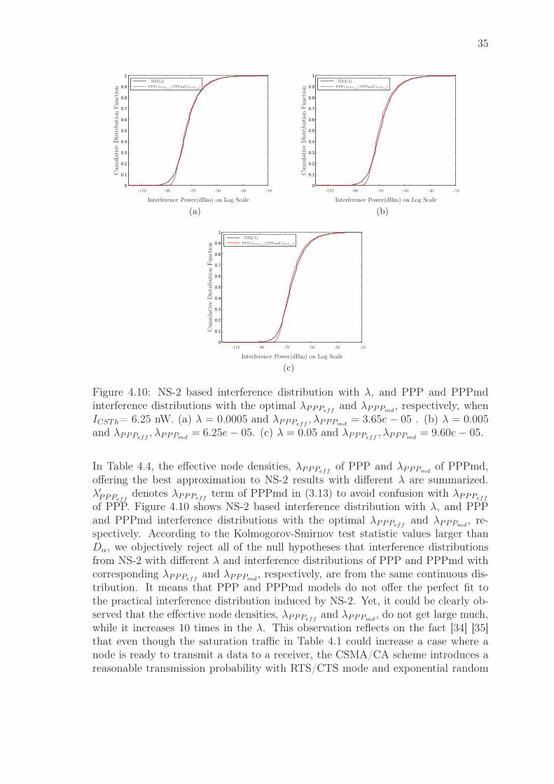
Figure 4.10: NS-2 based interference distribution with λ, and PPP and PPPmdinterference distributions with the optimal λPPPeff

and λPPPmd, respectively, when

ICSTh= 6.25 nW. (a) λ = 0.0005 and λPPPeff, λPPPmd

= 3.65e− 05 . (b) λ = 0.005and λPPPeff

, λPPPmd= 6.25e− 05. (c) λ = 0.05 and λPPPeff

, λPPPmd= 9.60e− 05.

In Table 4.4, the effective node densities, λPPPeffof PPP and λPPPmd

of PPPmd,offering the best approximation to NS-2 results with different λ are summarized.λ′

PPPeffdenotes λPPPeff

term of PPPmd in (3.13) to avoid confusion with λPPPeff

of PPP. Figure 4.10 shows NS-2 based interference distribution with λ, and PPPand PPPmd interference distributions with the optimal λPPPeff

and λPPPmd, re-

spectively. According to the Kolmogorov-Smirnov test statistic values larger thanDα, we objectively reject all of the null hypotheses that interference distributionsfrom NS-2 with different λ and interference distributions of PPP and PPPmd withcorresponding λPPPeff

and λPPPmd, respectively, are from the same continuous dis-

tribution. It means that PPP and PPPmd models do not offer the perfect fit tothe practical interference distribution induced by NS-2. Yet, it could be clearly ob-served that the effective node densities, λPPPeff

and λPPPmd, do not get large much,

while it increases 10 times in the λ. This observation reflects on the fact [34] [35]that even though the saturation traffic in Table 4.1 could increase a case where anode is ready to transmit a data to a receiver, the CSMA/CA scheme introduces areasonable transmission probability with RTS/CTS mode and exponential random

36

backoff scheme used in NS-2 simulation, making an effect on effective node geometry.

4.5.3 Extrapolation Analysis

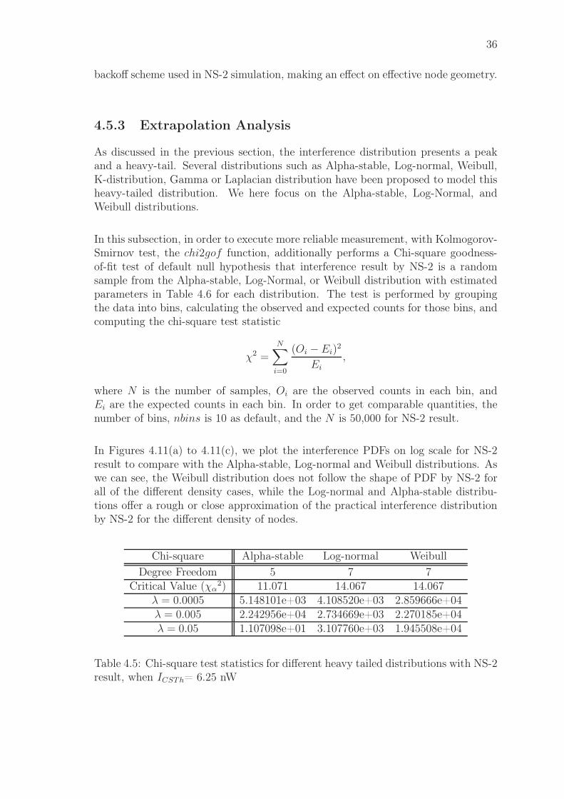
As discussed in the previous section, the interference distribution presents a peakand a heavy-tail. Several distributions such as Alpha-stable, Log-normal, Weibull,K-distribution, Gamma or Laplacian distribution have been proposed to model thisheavy-tailed distribution. We here focus on the Alpha-stable, Log-Normal, andWeibull distributions.

In this subsection, in order to execute more reliable measurement, with Kolmogorov-Smirnov test, the chi2gof function, additionally performs a Chi-square goodness-of-fit test of default null hypothesis that interference result by NS-2 is a randomsample from the Alpha-stable, Log-Normal, or Weibull distribution with estimatedparameters in Table 4.6 for each distribution. The test is performed by groupingthe data into bins, calculating the observed and expected counts for those bins, andcomputing the chi-square test statistic

χ2 =

N∑

i=0

(Oi −Ei)2

Ei,

where N is the number of samples, Oi are the observed counts in each bin, andEi are the expected counts in each bin. In order to get comparable quantities, thenumber of bins, nbins is 10 as default, and the N is 50,000 for NS-2 result.

In Figures 4.11(a) to 4.11(c), we plot the interference PDFs on log scale for NS-2result to compare with the Alpha-stable, Log-normal and Weibull distributions. Aswe can see, the Weibull distribution does not follow the shape of PDF by NS-2 forall of the different density cases, while the Log-normal and Alpha-stable distribu-tions offer a rough or close approximation of the practical interference distributionby NS-2 for the different density of nodes.

Chi-square Alpha-stable Log-normal Weibull

Degree Freedom 5 7 7Critical Value (χα

2) 11.071 14.067 14.067λ = 0.0005 5.148101e+03 4.108520e+03 2.859666e+04λ = 0.005 2.242956e+04 2.734669e+03 2.270185e+04λ = 0.05 1.107098e+01 3.107760e+03 1.945508e+04

Table 4.5: Chi-square test statistics for different heavy tailed distributions with NS-2result, when ICSTh= 6.25 nW

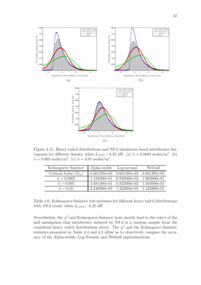
37

0

0.005

0.01

0.015

0.02

0.025

0.03

0.035

replacemen

Pro

bab

ility

Den

sity

Funct

ion

Interference Power(dBm) on Log Scale

alpha-stablelog-normalweibullNS2

-90 -70 -50 -30

(a)

0

0.005

0.01

0.015

0.02

0.025

0.03

0.035

Pro

bab

ility

Den

sity

Funct

ion

Interference Power(dBm) on Log Scale

alpha-stablelog-normalweibullNS2

-90 -70 -50 -30

(b)

0

0.005

0.01

0.015

0.02

0.025

0.03

0.035

Pro

bab

ility

Den

sity

Funct

ion

Interference Power(dBm) on Log Scale

alpha-stablelog-normalweibullNS2

-90 -70 -50 -30

(c)

Figure 4.11: Heavy tailed distributions and NS-2 simulation-based interference his-tograms for different density, when ICSTh= 6.25 nW. (a) λ = 0.0005 nodes/m2. (b)λ = 0.005 nodes/m2. (c) λ = 0.05 nodes/m2.

Kolmogorov-Smirnov Alpha-stable Log-normal Weibull

Critical Value (Dα) 8.601395e-03 8.601395e-03 8.601395e-03λ = 0.0005 1.182000e-01 8.932000e-02 1.860800e-01λ = 0.005 1.681400e-01 6.822000e-02 1.564000e-01λ = 0.05 8.240000e-03 7.222000e-02 1.442800e-01

Table 4.6: Kolmogorov-Smirnov test statistics for different heavy tailed distributionswith NS-2 result, when ICSTh= 6.25 nW

Nevertheless, the χ2 and Kolmogorov-Smirnov tests mostly lead to the reject of thenull assumption that interference induced by NS-2 is a random sample from theconsidered heavy tailed distributions above. The χ2 and the Kolmogorov-Smirnovstatistics presented in Table 4.4 and 4.5 allow us to objectively compare the accu-racy of the Alpha-stable, Log-Normal, and Weibull approximations.

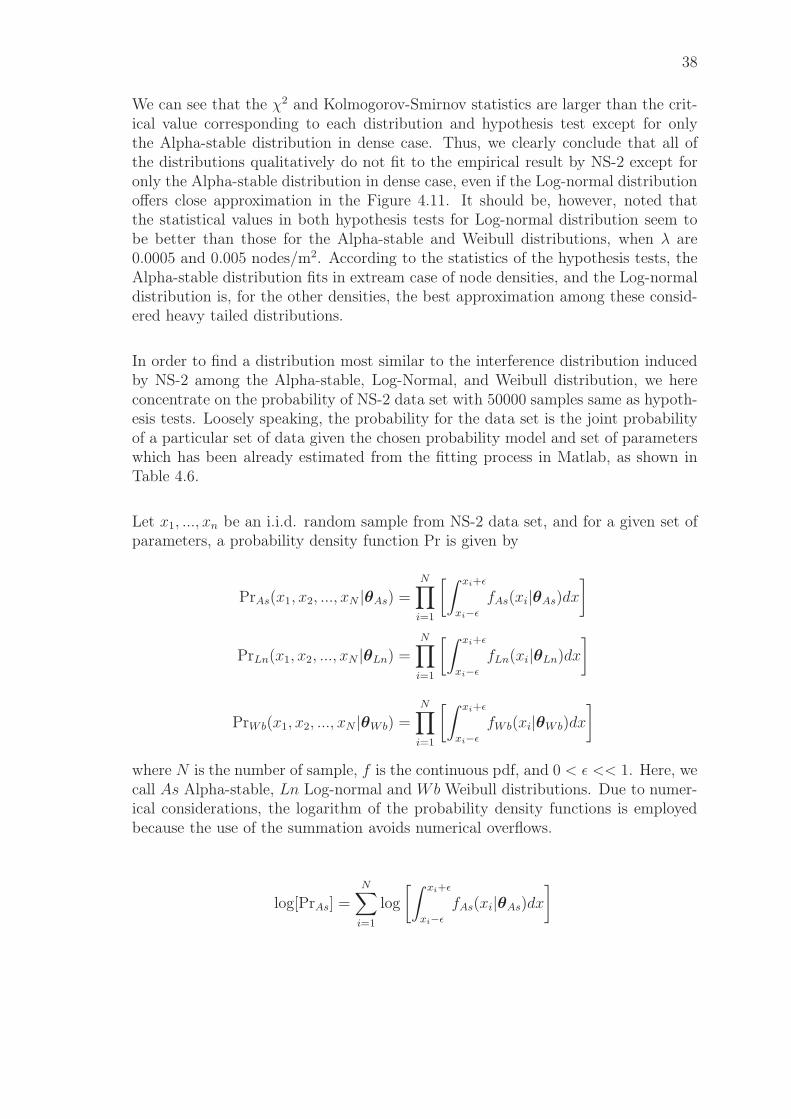
38

We can see that the χ2 and Kolmogorov-Smirnov statistics are larger than the crit-ical value corresponding to each distribution and hypothesis test except for onlythe Alpha-stable distribution in dense case. Thus, we clearly conclude that all ofthe distributions qualitatively do not fit to the empirical result by NS-2 except foronly the Alpha-stable distribution in dense case, even if the Log-normal distributionoffers close approximation in the Figure 4.11. It should be, however, noted thatthe statistical values in both hypothesis tests for Log-normal distribution seem tobe better than those for the Alpha-stable and Weibull distributions, when λ are0.0005 and 0.005 nodes/m2. According to the statistics of the hypothesis tests, theAlpha-stable distribution fits in extream case of node densities, and the Log-normaldistribution is, for the other densities, the best approximation among these consid-ered heavy tailed distributions.

In order to find a distribution most similar to the interference distribution inducedby NS-2 among the Alpha-stable, Log-Normal, and Weibull distribution, we hereconcentrate on the probability of NS-2 data set with 50000 samples same as hypoth-esis tests. Loosely speaking, the probability for the data set is the joint probabilityof a particular set of data given the chosen probability model and set of parameterswhich has been already estimated from the fitting process in Matlab, as shown inTable 4.6.

Let x1, ..., xn be an i.i.d. random sample from NS-2 data set, and for a given set ofparameters, a probability density function Pr is given by

PrAs(x1, x2, ..., xN |θAs) =

N∏

i=1

[∫ xi+ǫ

xi−ǫ

fAs(xi|θAs)dx

]

PrLn(x1, x2, ..., xN |θLn) =N∏

i=1

[∫ xi+ǫ

xi−ǫ

fLn(xi|θLn)dx

]

PrWb(x1, x2, ..., xN |θWb) =

N∏

i=1

[∫ xi+ǫ

xi−ǫ

fWb(xi|θWb)dx

]

where N is the number of sample, f is the continuous pdf, and 0 < ǫ << 1. Here, wecall As Alpha-stable, Ln Log-normal and Wb Weibull distributions. Due to numer-ical considerations, the logarithm of the probability density functions is employedbecause the use of the summation avoids numerical overflows.

log[PrAs] =N∑

i=1

log

[∫ xi+ǫ

xi−ǫ

fAs(xi|θAs)dx

]

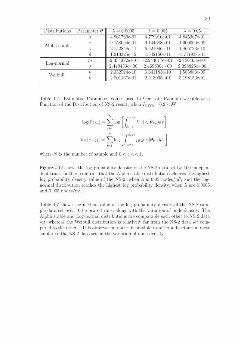
39

Distributions Parameter θ λ = 0.0005 λ = 0.005 λ = 0.05

Alpha-stable

α 4.961760e-01 4.779910e-01 4.845367e-01β 9.158094e-01 9.144688e-01 1.000000e-00γ 2.152848e-11 6.521046e-11 1.466723e-10δ 1.213325e-12 1.542156e-11 -1.711938e-11

Log-normalm -2.354072e+01 -2.243617e+01 -2.156463e+01σ 2.449433e+00 2.469530e+00 2.398825e+00

Weibullν 2.352524e-10 6.641183e-10 1.585883e-09k 2.801167e-01 2.913005e-01 3.198153e-01

Table 4.7: Estimated Parameter Values used to Generate Random variable as aFunction of the Distribution of NS-2 result, when ICSTh= 6.25 nW

log[PrLn] =

N∑

i=1

log

[∫ xi+ǫ

xi−ǫ

fLn(xi|θLn)dx

]

log[PrWb] =

N∑

i=1

log

[∫ xi+ǫ

xi−ǫ

fWb(xi|θWb)dx

]

where N is the number of sample and 0 < ǫ << 1.

Figure 4.12 shows the log probability density of the NS-2 data set by 100 indepen-dent trials, further, confirms that the Alpha-stable distribution achieves the highestlog probability density value of the NS-2, when λ is 0.05 nodes/m2, and the log-normal distribution reaches the highest log probability density, when λ are 0.0005and 0.005 nodes/m2.

Table 4.7 shows the median value of the log probability density of the NS-2 sam-ple data set over 100 repeated runs, along with the variation of node density. TheAlpha stable and Log-normal distributions are comparable each other to NS-2 dataset, whereas the Weibull distribution is relatively far from the NS-2 data set com-pared to the others. This observation makes it possible to select a distribution mostsimilar to the NS-2 data set on the variation of node density.

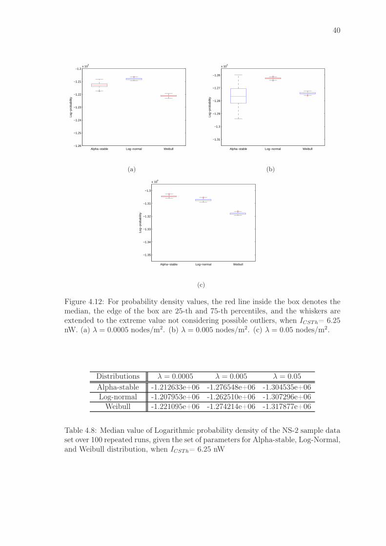
40

−1.26

−1.25

−1.24

−1.23

−1.22

−1.21

−1.2x 10

6

Alpha−stable Log−normal Weibull

Log−

prob

abili

ty

(a)

−1.31

−1.3

−1.29

−1.28

−1.27

−1.26

x 106

Alpha−stable Log−normal Weibull

Log−

prob

abili

ty

(b)

−1.35

−1.34

−1.33

−1.32

−1.31

−1.3

x 106

Alpha−stable Log−normal Weibull

Log−

prob

abili

ty

(c)

Figure 4.12: For probability density values, the red line inside the box denotes themedian, the edge of the box are 25-th and 75-th percentiles, and the whiskers areextended to the extreme value not considering possible outliers, when ICSTh= 6.25nW. (a) λ = 0.0005 nodes/m2. (b) λ = 0.005 nodes/m2. (c) λ = 0.05 nodes/m2.

Distributions λ = 0.0005 λ = 0.005 λ = 0.05

Alpha-stable -1.212633e+06 -1.276548e+06 -1.304535e+06Log-normal -1.207953e+06 -1.262510e+06 -1.307296e+06

Weibull -1.221095e+06 -1.274214e+06 -1.317877e+06

Table 4.8: Median value of Logarithmic probability density of the NS-2 sample dataset over 100 repeated runs, given the set of parameters for Alpha-stable, Log-Normal,and Weibull distribution, when ICSTh= 6.25 nW

Chapter 5

Conclusions and Future Work

In this chapter we are going to conclude the main results achieved in this thesis.Most importantly, some possible future research directions based on this thesis arediscussed as well.

5.1 Conclusions

As interference results from the summation of signals issued by concurrent trans-mitters, it directly depends on the nodes location. Thus, the point process used tomodel concurrent nodes location is fundamental in any multi-hop wireless networkresearch. Assuming the active transmitters are distributed according to a hardcoreprocess, the PPP with modified density, MPP, and SSI are discussed for CSMA/CAnetworks where a busy medium detection depends on the aggregated power from allconcurrent signals.

For very sparse networks, the PPP with modified density, MPP, and SSI, tend tobe similar to the result of PPP, since the PPP does not consider any dependencybetween the transmitter location. For denser case, various point processes lead todifferent interference distributions. Noticeably, the difference between MPP and SSIgets large, due to the under-estimated density issue. In the practical interferencedistribution itself induced by NS-2, node density variation lead to shift of peak point.

We point out, however, that the interference distributions generated by the var-ious point processes are significantly different with the practical results by NS-2.The existence of large gap is mainly due to the assumption that all of the pointprocess models only consider multiple concurrently active node, whereas in NS-2,the active node, the probability of medium access of a typical node is not givena priori and it has to be determined by the CSMA/CA DCF policy. In addition,Kolmogorov-Smirnov test executed to ensure objective comparison with statistic

41

42

values, result in the rejection of the assumption that interference distributions fromNS-2 and each of point processes are from the same continuous distribution. Evenunder consideration of the effective node densities offering the best approximationto the interference distribution by NS-2, the hypothesis test leads to the rejectionagain. However, the statistics of the hypothesis test allow us to confirm that theCSMA/CA scheme introduces a reasonable transmission probability with RTS/CTSmode and exponential random backoff scheme, making an effect on effective nodegeometry.

Nevertheless, we have observed that all of the interference distributions by NS-2 andProcesses all offer the similar shape which follows a peak and an asymmetry witha more or less heavy tail depending on each mean and variance. This observationabsolutely contradicts a classical assumption in which the interference is generallyconsidered to be Gaussian. We show that in the case where some of the interferersare dominant, the central limit theorem(CLT) is not valid any more, even if thenumber of interferers may be large. We further confirm that in a case which gets ridof dominant interference, the distribution has a tendency similar to the Gaussianshape.

Besides, this observation has promoted an interest in characterizing the distribu-tion of the aggregated interference with the Log-normal, Alpha-stable, and Weibulldistributions as a family of heavy tail distributions. Through the fitting plot, theempirical interference distributions by NS-2 are approximated by the Alpha stableand Log-normal distribution for the different densities of nodes. However, the χ2

and Kolmogorov-Smirnov tests have mostly led to the reject of the null assumptionthat the interference result by NS-2 is a random sample from the Alpha-stable, Log-Normal, or Weibull distribution with estimated parameters except for the Alpha-stable distribution in high node density. The hypothesis statistics from these testssystematically yield agreement on the choice of the better approximation. Addition-ally, the log probability process with several iterations certainly makes it possible tomore reliably select a distribution among the considered 3 kind of the heavy taileddistributions most similar to the NS-2 data set on the variation of node density.This approximation provides the opportunity to analytically study and characterizevalues such as SINR which is used to specify and ultimately compute the connec-tivity/coverage and the capacity/throughput.

5.2 Possible Future Work

Interesting research topics about spatial model based on stochastic geometry forinterference are below

• to build a more realistic modelling to consider the concurrently transmitting

43

node density without pre-assumption which most of point processes shouldemploy. In order to make it possible, we are able to begin with transmissionprobability Biancchi introduced for MAC performance measurement.

• to derive new distribution closest to practical interference or find some trend ofparameters representing for theoretical distribution along with various factorssuch as density, CS range, RTS/CTS usage, or channel parameters.

• to apply this spatial model for interference to different type of wireless networkssuch as Cognitive radio and Femtocells as well as Ad hoc networks. When itcomes to Cognitive Radio, a primary consideration of a cognitive radio is thelikelihood of interfering with a primary. The probability of this occurring mustbe held small, and it clearly depends on the spatial density and the typicallyunknown locations of the primary receivers. Stochastic geometry provides anessential toolkit for understanding femtocell deployments. A natural modelfor two-tier networks consisting of tier 1 base stations and tier 2 femtocells isto model the femtocell locations as a point process of density lf overlaying aregular grid of base stations.

Bibliography

[1] F. Baccelli, B. Blaszczyszyn, and P. Muhlethaler, "An Aloha protocol for multi-hop mobile wireless networks," IEEE Trans. Information Theory, vol.52, no.2,pp. 421- 436, Feburary 2006

[2] Y.-C. Cheng and T.G. Robertazzi, "A new spatial point process for multi-hop radio network modeling," Proc. 1990 IEEE International Conf. Comm.,pp.1241-1245

[3] A. Busson and G. Chelius, "Point processes for interference modeling in CS-MA/CA ad-hoc networks," In Proceedings of the 6th ACM symposium on Per-formance evaluation of wireless ad hoc, sensor, and ubiquitous networks (PE-WASUN ’09). ACM, New York, NY, USA, 33-40. 2009

[4] D. Stoyan, W. Kendall, and J. Mecke, Stochastic Geometry and Its Applications,2nd Edition. John Wiley ans Sons Ltd, Chichester, UK, 1996

[5] A. Busson, "An overview of results on ad hoc network performances usingspatial model" IEEE Symposium, Computers and Communications, vol., no.,pp.36-41, 5-8 July 2009 doi: 10.1109/ISCC.2009.5202409

[6] D. Tse and P. Viswanath, Fundamentals of wireless communication. CambridgeUniversity Press, 2005

[7] M. Veillette. Stable distribution Matlab package. Boston university. Availableon http://math.bu.edu/people/mveillet/

[8] F. Baccelli and B. Bartek, "Stochastic Geometry and Wireless Networks Volume1: Theory," Foundations and Trends in Networking, vol. 3, no. 3-4, pp. 249-449,2009

[9] E.S. Sousa and J.A. Silvester, "Optimum transmission ranges in a direct-sequence spread spectrum multihop packet radio network", IEEE Journal onSelected Areas in Commun., Vol. 8, No. 5, pp. 762-771, 1990

[10] X. Yang and N. Vaidya, "On physical carrier sensing in wireless ad hoc net-works", in IEEE Proc. Computer Commun., 2005

44

45

[11] T.S. Kim, H. Lim, and J.C. Hou.; , "Improving spatial reuse through tuningtransmit power, carrier sense threshold, and data rate in multihop wirelessnetworks", In Proceedings of the 12th annual international conference on Mobilecomputing and networking ACM, New York, NY, USA, 366-377. 2006

[12] I. Palasti, "On some random space filling problem". Mathematical Institute ofHungarian Academy of Sciences, 5(1):353.359, 1960

[13] F. Baccelli and B. Blaszczyszyn; "On a coverage process ranging from theboolean model to the poisson voronoi tessellation, with applications to wirelesscommunications." Advances in Applied Probability, 33:293-323, 2001

[14] F. Baccelli, B. Blaszczyszyn, and F. Tournois; , "Spatial averages of coveragecharacteristics in large cdma networks". Wireless Networks, 8(6):569-586, 2002

[15] O. Dousse, F. Baccelli, and P. Thiran, "Impact of interferences on connectivityin ad hoc networks," IEEE/ACM Trans. Networking, vol.13, no.2, pp. 425- 436,April 2005

[16] J. Ilow and D. Hatzinakos, "Analytic alpha-stable noise modeling in a Poissonfield of interferers or scatterers," IEEE Trans. Signal Processing, vol.46, no.6,pp.1601-1611, June 1998

[17] X. Yang and A.P. Petropulu, "Co-channel interference modeling and analysis ina Poisson field of interferers in wireless communications," IEEE Trans. SignalProcessing, vol.51, no.1, pp. 64- 76, January 2003

[18] P. Cardieri, "Modeling Interference in Wireless Ad Hoc Networks," IEEE Com-munications Surveys & Tutorials, vol.12, no.4, pp.551-572, Fourth Quarter 2010

[19] J. Venkataraman, M. Haenggi, and O. Collins, "Shot Noise Models for Outageand Throughput Analyses in Wireless Ad Hoc Networks," MILCOM, pp. 1-7,2006

[20] A. Busson, G. Chelius, and J.-M. Gorce, "Interference modeling in CSMAmulti-hop wireless networks," INRIA, Research Report 6624.

[21] M. Haenggi, J.G. Andrews, F. Baccelli, O. Dousse, and M. Franceschetti,"Stochastic geometry and random graphs for the analysis and design of wirelessnetworks". IEEE J.Sel. A. Commun. 27, 1029-1046, September 2009

[22] A.O. Allen, Probability, Statistics, And Queueing Theory with Computer Sci-ence Applications. Academic Press, 1978

[23] L. Le Cam, "The central limit theorem around 1935," Stat. Sci., vol.1, no.1,pp. 78-91, February 1986

[24] "Network Simulator ns-2," http://www.isi.edu/nsnam/ns/.

46

[25] "IEEE Std. 802.11-2007, Part 11: Wireless LAN Medium Access Control(MAC) and Physical Layer (PHY) specifications," IEEE Std. 802.11, 2007

[26] Q. Chen, F. Schmidt-Eisenlohr, D.Jiang, M. Torrent-Moreno, L. Delgrossi, andH. Hartenstein, "Overhaul of ieee 802.11 modeling and simulation in ns-2",Proceedings of the 10th ACM Symposium on Modeling, analysis, and simulationof wireless and mobile systems, Chania, Crete Island, Greece, October 22-26,2007

[27] J. Hwang and S.L. Kim, "Cross-Layer Optimization and Network Codingin CSMA/CA-Based Wireless Multihop Networks," Trans. on Netw., [On-line]http://ieeexplore.ieee.org/stamp/stamp.jsp?tp=&arnumber=5675760,DOI 10.1109/TNET.2010.2096430

[28] F. Baccelli and B. Bartek, "Stochastic Geometry and Wireless Networks Volume2: Applications," Foundations and Trends in Networking, vol. 4, no. 1-2, pp.1-312, 2009

[29] Kevin Fall and Kannan Varadhan, "The ns Manual (formerly ns Notes andDocumentation)", March 2007

[30] J. S. Evans and D. Everitt, "On the teletraffic capacity of CDMA cellularnetworks," IEEE Trans. Veh. Technol., vol. 48, no. 1, pp. 153-165, January1999

[31] M. Z. Win, P. C. Pinto, and L. A. Shepp; , "A mathematical theory of net-work interference and its applications," Proc. IEEE, vol. 97, no. 2, pp. 205-230,February 2009

[32] A. Ghasemi and E. S. Sousa, "Interference aggregation in spectrum-sensingcognitive wireless networks," IEEE J. Sel. Topics Signal Process., vol. 2, no. 1,pp. 41-56, February 2008

[33] M. Aljuaid and H. Yanikomeroglu, "Investigating the Gaussian Convergence ofthe Distribution of the Aggregate Interference Power in Large Wireless Net-works," Vehicular Technology, IEEE Transactions on , vol.59, no.9, pp.4418-4424, November 2010

[34] G. Bianchi, "Performance analysis of the ieee 802.11 distributed coordinationfunction," IEEE Journal, Selected Areas in Communications, vol. 18, no. 3, pp.535-547, 2000

[35] H. Wu, Y. Peng, K. Long, and J. Ma; , "Performance of Reliable TransportProtocol over IEEE 802.11 Wireless LAN: Analysis and Enhancement," in Pro-ceeding of the IEEE Conference on Computer Communications (INFOCOM),New York, NY, June 2002

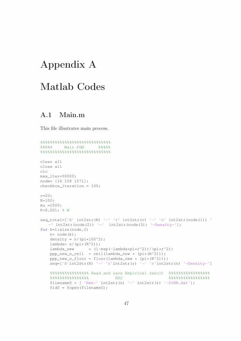
Appendix A

Matlab Codes

A.1 Main.m

This file illustrates main process.

%%%%%%%%%%%%%%%%%%%%%%%%%%%%%%%%%% Main PGM %%%%%%%%%%%%%%%%%%%%%%%%%%%%%%%%%%

clear allclose allclcmax_iter=50000;node= [16 158 1571];checkbox_iteration = 100;

r=20;R=100;mu =1000;P=0.001; % W

seq_total=[ 'R' int2str(R) '-' 'r' int2str(r) '-' 'n' int2str(node(1)) '-' int2str(node(2)) '-' int2str(node(3)) '-Density-' ];

for k=1:size(node,2)n= node(k);density = n/(pi * 100^2);lambda= n/(pi * (R^2));lambda_new = (1-exp(-lambda * pi * r^2))/(pi * r^2);ppp_new_n_ceil = ceil(lambda_new * (pi * (R^2)));ppp_new_n_floor = floor(lambda_new * (pi * (R^2)));seq=[ 'R' int2str(R) '-' 'r' int2str(r) '-' 'n' int2str(n) '-Density-' ]

%%%%%%%%%%%%%%%% Read and save Empirical result %%%%%%%%%%%%%%%%%%%%%%%%%%%%%%%%% NS2 %%%%%%%%%%%%%%%%%filename0 = [ 'Den-' int2str(n) '-' int2str(r) '-SINR.dat' ];fid0 = fopen(filename0);

47

48

Total_interference_data = textscan(fid0, '%f' );fclose(fid0);Total_interference = Total_interference_data{1};sort_inf=sort(Total_interference, 'ascend' );index = find(sort_inf ≤0.000);interf= (sort_inf(size(index)+1: end ) * (10^(-12)));min_x = log10(min(interf));max_x = log10(max(interf));interval = min_x:0.05:max_x;x= 10.^interval;

%%%%%%%%%%%%%%%%%%% Theoretical closed form %%%%%%%%%%%%%%%%%%%%%%%%%%%%%%%%%% PPP & Modified_PPP %%%%%%%%%%%%%%%% PPPppp_theo=erfc((lambda * pi^2) ./ (4 * sqrt(mu * ppp_theo_x)));ppp_theo_cdf_hist_percent = ppp_theo;ppp_theo(2: end) = ppp_theo(2: end) - ppp_theo(1: end -1);ppp_theo_pdf_hist_percent = ppp_theo;% PPPmdppp_modified_theo=erfc((lambda_new * pi^2) ./ ...

(4 * sqrt(mu * ppp_theo_x)));ppp_modified_theo_cdf_hist_percent = ppp_modified_the o;ppp_modified_theo(2: end ) = ppp_modified_theo(2: end ) - ...

ppp_modified_theo(1: end-1);ppp_modified_theo_pdf_hist_percent = ppp_modified_the o;

%%%%%%%%%%%%%%%%%%% Simulation %%%%%%%%%%%%%%%%%%%%%%%%%% PPP & PPPmd & Matern & SSI %%%%%%%ppp_interf = [];ppp_new_interf_ceil = [];ppp_new_interf_floor = [];matern_interf = [];ssi_interf = [];for a=1:max_iter

%%%%%%%%%%%%%%%%%% Node distribution %%%%%%%%%%%%%%%%%%% PPPppp_theta=rand(1,n) * 2* pi;ppp_dist=R * sqrt(rand(1,n));ppp_mother_node=[ppp_theta;ppp_dist];% PPPmd_ceilppp_new_theta_ceil=rand(1,ppp_new_n_ceil) * 2* pi;ppp_new_dist_ceil=R * sqrt(rand(1,ppp_new_n_ceil));ppp_new_mother_node_ceil= ...

[ppp_new_theta_ceil;ppp_new_dist_ceil];% PPPmd_floorppp_new_theta_floor=rand(1,ppp_new_n_floor) * 2* pi;ppp_new_dist_floor=R * sqrt(rand(1,ppp_new_n_floor));ppp_new_mother_node_floor= ...

[ppp_new_theta_floor;ppp_new_dist_floor];% Materntheta=rand(1,n) * 2* pi;

49

dist=R * sqrt(rand(1,n));mother_node=[theta;dist];matern_selec=mother_node(:,1);matern_counter_node=mother_node(:,1);for i=2:n

matern_fail=sum(sqrt(dist(i)^2+ ...matern_counter_node(2,:).^2- ...

2* dist(i). * matern_counter_node(2,:). * ...cos(theta(i)-matern_counter_node(1,:)))<r);

if matern_fail==0;matern_selec=[matern_selec,mother_node(:,i)];

endmatern_counter_node= ...

[matern_counter_node,mother_node(:,i)];end%SSIssi_selec=mother_node(:,1);for i=2:1:n

ssi_fail=sum(sqrt(dist(i)^2+ssi_selec(2,:).^2- ...2* dist(i). * ssi_selec(2,:). * ...cos(theta(i)-ssi_selec(1,:)))<r);

if ssi_fail==0;ssi_selec=[ssi_selec,mother_node(:,i)];

endend

%%%%%%%%%%%%%%%%%% Channel model %%%%%%%%%%%%%%%%%%% PPPppp_X=-log(1-rand(1,size(ppp_mother_node,2)));ppp_l=P * ppp_X. * min(1,ppp_mother_node(2,:).^(-4));ppp_interf = [ppp_interf sum(ppp_l)];% PPPmd_ceilppp_new_X_ceil= ...-log(1-rand(1,size(ppp_new_mother_node_ceil,2)));ppp_new_l_ceil= ...P* ppp_new_X_ceil. * min(1,ppp_new_mother_node_ceil(2,:).^(-4));ppp_new_interf_ceil = ...[ppp_new_interf_ceil sum(ppp_new_l_ceil)];% PPPmd_floorppp_new_X_floor= ...-log(1-rand(1,size(ppp_new_mother_node_floor,2)));ppp_new_l_floor= P * ppp_new_X_floor. * min(1,

ppp_new_mother_node_floor(2,:).^(-4));ppp_new_interf_floor = [ppp_new_interf_floor sum(

ppp_new_l_floor)];% Maternmatern_X=-log(1-rand(1,size(matern_selec,2)));matern_l=P * matern_X. * min(1,matern_selec(2,:).^(-4));matern_interf = [matern_interf sum(matern_l)];% SSIssi_X=-log(1-rand(1,size(ssi_selec,2)));ssi_l=P * ssi_X. * min(1,ssi_selec(2,:).^(-4));ssi_interf = [ssi_interf sum(ssi_l)];

50

%%%%%%%%%%%%%%%%%% Erase memory %%%%%%%%%%%%%%%%%%clear ppp_theta ppp_dist ppp_mother_node;clear ppp_new_theta ppp_new_dist;clear ppp_new_mother_node ppp_new_theta_floor;clear ppp_new_dist_floor;clear ppp_new_mother_node_floor ppp_X ppp_l;clear ppp_new_X ppp_new_l;clear ppp_new_X_floor ppp_new_l_floor;clear theta dist mother_node i;clear matern_selec clear matern_fail;clear matern_X matern_l;clear ssi_selec ssi_fail ssi_X ssi_l;

end

%%%%%%%%%%%%%%%%%%% PDF and CDF %%%%%%%%%%%%%%%%%%%%%%% NS2 & PPP & PPPmd & Matern & SSI %%%%% NS2pdf_hist = histc(interf,x);pdf_hist_sum = max(cumsum(pdf_hist));pdf_hist_percent = pdf_hist / pdf_hist_sum;cdf_hist_percent = (cumsum(pdf_hist)/ pdf_hist_sum);ppp_theo_interval = interval;ppp_theo_x= x;extrapolation( 'ns2' ,interf, R, r, n,max_iter );% PPPppp_pdf_hist = histc(ppp_interf,x);ppp_pdf_hist_cumsum = cumsum(ppp_pdf_hist);ppp_pdf_hist_sum = max(ppp_pdf_hist_cumsum);ppp_pdf_hist_percent = ppp_pdf_hist/ppp_pdf_hist_sum;ppp_cdf_hist = cumsum(ppp_pdf_hist);ppp_cdf_hist_max = max(ppp_cdf_hist);ppp_cdf_hist_percent = (ppp_cdf_hist/ppp_cdf_hist_max );% PPPmd_ceilppp_new_pdf_hist_ceil = histc(ppp_new_interf_ceil,x);ppp_new_pdf_hist_cumsum_ceil = cumsum(ppp_new_pdf_his t_ceil);ppp_new_pdf_hist_sum_ceil = max(ppp_new_pdf_hist_cums um_ceil);ppp_new_pdf_hist_percent_ceil = ppp_new_pdf_hist_ceil /

ppp_new_pdf_hist_sum_ceil;ppp_new_cdf_hist_ceil = cumsum(ppp_new_pdf_hist_ceil) ;ppp_new_cdf_hist_max_ceil = max(ppp_new_cdf_hist_ceil );ppp_new_cdf_hist_percent_ceil = (ppp_new_cdf_hist_cei l/

ppp_new_cdf_hist_max_ceil);% PPPmd_floorppp_new_pdf_hist_floor = histc(ppp_new_interf_floor,x );ppp_new_pdf_hist_cumsum_floor = cumsum(ppp_new_pdf_hi st_floor);ppp_new_pdf_hist_sum_floor = max(ppp_new_pdf_hist_cum sum_floor);ppp_new_pdf_hist_percent_floor = ppp_new_pdf_hist_flo or/

ppp_new_pdf_hist_sum_floor;ppp_new_cdf_hist_floor = cumsum(ppp_new_pdf_hist_floo r);ppp_new_cdf_hist_max_floor = max(ppp_new_cdf_hist_flo or);ppp_new_cdf_hist_percent_floor = ppp_new_cdf_hist_flo or/

ppp_new_cdf_hist_max_floor;% matern

51

matern_pdf_hist = histc(matern_interf,x);matern_pdf_hist_cumsum = cumsum(matern_pdf_hist);matern_pdf_hist_sum = max(matern_pdf_hist_cumsum);matern_pdf_hist_percent = matern_pdf_hist/matern_pdf_ hist_sum;matern_cdf_hist = cumsum(matern_pdf_hist);matern_cdf_hist_max = max(matern_cdf_hist);matern_cdf_hist_percent = (matern_cdf_hist/matern_cdf _hist_max);% ssissi_pdf_hist = histc(ssi_interf,x);ssi_pdf_hist_cumsum = cumsum(ssi_pdf_hist);ssi_pdf_hist_sum = max(ssi_pdf_hist_cumsum);ssi_pdf_hist_percent = ssi_pdf_hist/ssi_pdf_hist_sum;ssi_cdf_hist = cumsum(ssi_pdf_hist);ssi_cdf_hist_max = max(ssi_cdf_hist);ssi_cdf_hist_percent = (ssi_cdf_hist/ssi_cdf_hist_max );

%%%%%%%%%%%%%%% Kolmogorov-Smirnov Test %%%%%%%%%%%%%%%%%%%% NS2 vs (PPP || PPPmd || Matern || SSI) %%%%%[h1,p1,k1]=kstest2(interf, ppp_interf);[h2,p2,k2]=kstest2(interf, ppp_new_interf_ceil);[h3,p3,k3]=kstest2(interf, matern_interf);[h4,p4,k4]=kstest2(interf, ssi_interf);PP = [ 'R' int2str(R) '-r' int2str(r) '-n' int2str(n) '-Static-

kstest' ];filename0=[ PP '-ns2-process.txt' ];fid = fopen(filename0, 'wt' );fprintf(fid, filename0);fprintf(fid, '\nns2 vs ppp h= %d\n' , h1);fprintf(fid, 'ns2 vs ppp p= %d\n' , p1);fprintf(fid, 'ns2 vs ppp k= %d\n' , k1);fprintf(fid, 'ns2 vs cm h= %d\n' , h2);fprintf(fid, 'ns2 vs cm p= %d\n' , p2);fprintf(fid, 'ns2 vs cm k= %d\n' , k2);fprintf(fid, 'ns2 vs tm h= %d\n' , h3);fprintf(fid, 'ns2 vs tm p= %d\n' , p3);fprintf(fid, 'ns2 vs tm k= %d\n' , k3);fprintf(fid, 'ns2 vs ssi h= %d\n' , h4);fprintf(fid, 'ns2 vs ssi p= %d\n' , p4);fprintf(fid, 'ns2 vs ssi k= %d\n' , k4);fclose(fid);

%%%%%%%%%%%%%%% Extrapolation process %%%%%%%%%%%%%%%%%%%% NS2 vs heavy tailed distribution %%%%%extrapolation(checkbox_iteration, interf,max_iter,R, r, n);

%%%%%%%%%%%%%%% Figure generation %%%%%%%%%%%%%%%%%%%% PDF & CDF %%%%%% Set filename to save figures into * .fig filesfilename1=[ seq 'PDF-Normscale-Process' ];filename2=[ seq 'CDF-Logscale-Process' ];filename3=[ seq 'PDF-Normscale-Process-ns2' ];

52

filename4=[ seq 'CDF-Logscale-Process-ns2' ];filename5=[ seq_total 'PDF-Normscale' ];filename6=[ seq_total 'CDF-Logscale' ];fignumber1= (n)+1;fignumber2= (n)+2;fignumber3= (n)+3;fignumber4= (n)+4;

% PDF-Normscale for Comparison among Processes)fig1=figure(fignumber1);plot(x,ppp_pdf_hist_percent, '--' , 'Color' ,[0 0 1], 'LineWidth' ,2);hold on;plot(x,ppp_new_pdf_hist_percent_ceil, '-' , 'Color' ,[0 .5 0], '

LineWidth' ,2);hold on;plot(x,matern_pdf_hist_percent, '-.' , 'Color' ,[1 0 0], 'LineWidth' ,2);hold on;plot(x,ssi_pdf_hist_percent, ':' , 'Color' ,[0 0 0] , 'LineWidth' ,2);legend( 'PPP' , 'PPPmd' , 'MPP' , 'SSI' , 'Location' , 'NorthEast' );grid off;xlim([min(x) (1 * 10^(-8))]);xlabel( 'Power(W) on Normal Scale' );ylabel( 'Probability Density Function' );saveas(fig1,filename1, 'fig' );

% CDF-Logscale for Comparison among Processes)fig2=figure(fignumber2);semilogx(x,ppp_cdf_hist_percent , '--' , 'Color' ,[0 0 1], 'LineWidth'

,2);hold on;semilogx(x,ppp_new_cdf_hist_percent_ceil, '-' , 'Color' ,[0 .5 0], '

LineWidth' ,2);hold on;semilogx(x,matern_cdf_hist_percent, '-.' , 'Color' ,[1 0 0], 'LineWidth'

,2);hold on;semilogx(x,ssi_cdf_hist_percent, ':' , 'Color' ,[0 0 0] , 'LineWidth'

,2);legend( 'PPP' , 'PPPmd' , 'MPP' , 'SSI' , 'Location' , 'NorthWest' );xlim([10^(-11) 10^(-4)]);xlabel( 'Power(W) on Log Scale' );ylabel( 'Cummulative Distribution Function' );grid off;saveas(fig2,filename2, 'fig' );

% PDF-Normscale for Comparison among NS2 and Processesfig3=figure(fignumber3);plot(x,pdf_hist_percent , 'o' , 'Color' ,[0 0 0], 'LineWidth' ,2);hold on;plot(x,ppp_pdf_hist_percent, '--' , 'Color' ,[0 0 1], 'LineWidth' ,2);hold on;plot(x,ppp_new_pdf_hist_percent_ceil, '-' , 'Color' ,[0 .5 0], '

LineWidth' ,2);hold on;

53

plot(x,matern_pdf_hist_percent, '-.' , 'Color' ,[1 0 0], 'LineWidth' ,2);hold on;plot(x,ssi_pdf_hist_percent, ':' , 'Color' ,[0 0 0] , 'LineWidth' ,2);legend( 'NS2' , 'PPP' , 'PPPmd' , 'MPP' , 'SSI' , 'Location' , 'NorthEast' );grid off;xlim([min(x) (1 * 10^(-8))]);xlabel( 'Power(W) on Normal Scale' );ylabel( 'Probability Density Function' );saveas(fig3,filename3, 'fig' );

% CDF-Logscale for Comparison among NS2 and Processesfig4=figure(fignumber4);semilogx(x,cdf_hist_percent, 'o' , 'Color' ,[0 0 0], 'LineWidth' ,2);hold on;semilogx(x,ppp_cdf_hist_percent, '--' , 'Color' ,[0 0 1], 'LineWidth'

,2);hold on;semilogx(x,ppp_new_cdf_hist_percent_ceil, '-' , 'Color' ,[0 .5 0], '

LineWidth' ,2);hold on;semilogx(x,matern_cdf_hist_percent, '-.' , 'Color' ,[1 0 0], 'LineWidth'

,2);hold on;semilogx(x,ssi_cdf_hist_percent, ':' , 'Color' ,[0 0 0] , 'LineWidth'

,2);legend( 'NS2' , 'PPP' , 'PPPmd' , 'MPP' , 'SSI' , 'Location' , 'NorthEast' );xlim([10^(-11) 10^(-4)]);xlabel( 'Power(W) on Log Scale' );ylabel( 'Cummulative Distribution Function' );grid off;saveas(fig4,filename4, 'fig' );

% PDF-Normcale for Different densitiesfig5=figure(5);if k==1

plot(x,pdf_hist_percent, '--' , 'Color' ,[0 0 1], 'LineWidth' ,2);hold on;

elseif k==2plot(x,pdf_hist_percent, '-' , 'Color' ,[1 0 0], 'LineWidth' ,2);hold on;

elseplot(x,pdf_hist_percent, ':' , 'Color' ,[0 0 0], 'LineWidth' ,2);hold on;

endlegend( '\lambda=0.0005' , '\lambda=0.005' , '\lambda=0.05' );xlim([min(x) (1 * 10^(-9))]);xlabel( 'Power(W) on Normal Scale' );ylabel( 'Probability Density Function' );grid off;saveas(fig5,filename5, 'fig' );

% CDF-Normcale for Different densitiesfig6=figure(6);if k==1

54

semilogx(x,cdf_hist_percent, '--' , 'Color' ,[0 0 1], 'LineWidth',2);

hold on;elseif k==2

semilogx(x,cdf_hist_percent, '-' , 'Color' ,[1 0 0], 'LineWidth' ,2);

hold on;else

semilogx(x,cdf_hist_percent, ':' , 'Color' ,[0 0 0], 'LineWidth' ,2);

hold on;endxlim([10^(-13) 10^(-4)]);legend( '\lambda=0.0005' , '\lambda=0.005' , '\lambda=0.05' );xlabel( 'Power(W) on Log Scale' );ylabel( 'Cummulative Distribution Function' );grid off;saveas(fig6,filename6, 'fig' );

end % End for k=1:size(node,2)

55

A.2 Extrapolation2.m

This file illustrates extrapolation process.

%%%%%%%%%%%%%%%%%%%%%%%%%%%%%%%%%%%%%%%%%%%%%%% Extrapolation Process %%%%%%%%%%%%%%%%%%%%%%%%%%%%%%%%%%%%%%%%%%%%%%%function extrapolation(checkbox_iteration, long_interf, max_it er,R, r,

n)

epsilon = 1e-20;

%%%%%%%%%%%%%%%%%%% Check box generation %%%%%%%%%%%%%%%%%%%%%%% heavy tailed distribution %%%%%%for j=1 : checkbox_iteration

% Sampling 50000 * 2sampling_index = randsample(length(long_interf), max_i ter * 2);interf = long_interf(sampling_index(1:max_iter));interf_fitting = long_interf(sampling_index(max_iter+ 1: end));

% Estimate parameters for each distribution with raw datawbl(j,:) =wblfit(interf_fitting);p(j,:) = stblfit(interf_fitting, 'ecf' ,statset( 'Display' , 'iter'

))';parmhat(j,:)= lognfit(interf_fitting);[muhat,sigmahat] = normfit(interf_fitting);

% PDF for Alpha-stable fitalpha_x1 = stblcdf(interf + epsilon, p(j,1),p(j,2),p(j,3 ),p(j,4)

);alpha_x2 = stblcdf(interf - epsilon, p(j,1),p(j,2),p(j,3 ),p(j,4)

);probs_alpha = max(alpha_x1 - alpha_x2, 0);

% PDF for Log-normal fitlogn_x1 = logncdf(interf+ epsilon ,parmhat(j,1),parmhat (j,2));logn_x2 = logncdf(interf- epsilon ,parmhat(j,1),parmhat (j,2));probs_logn = max(logn_x1-logn_x2, 0);

% PDF for Weibull fitwbl_x1 = wblcdf(interf+ epsilon, wbl(j,1),wbl(j,2));wbl_x2 = wblcdf(interf- epsilon, wbl(j,1),wbl(j,2));probs_wbl = max(wbl_x1- wbl_x2, 0);probs_alpha( probs_alpha == 0) = 1e-20;probs_logn( probs_logn == 0) = 1e-20;probs_wbl( probs_wbl == 0) = 1e-20;

% Summation to avoid numerical overflowsProb_ML_alpha(j,1) =(sum(log(probs_alpha)));Prob_ML_logn(j,1) =(sum(log(probs_logn)));Prob_ML_wbl(j,1) =(sum(log(probs_wbl)));

56

% Save the variablessavevars.wbl(j,:) = wbl(j,:);savevars.p(j,:) = p(j,:);savevars.parmhat(j,:) = parmhat(j,:);savevars.Prob_alpha(j) = Prob_ML_alpha(j);savevars.Prob_logn(j) = Prob_ML_logn(j);savevars.Prob_wbl(j) = Prob_ML_wbl(j);

end

%%%%%%%%%%%%%%%%%%% Chi-square2 %%%%%%%%%%%%%%%%%%%%%%% heavy tailed distribution %%%%%%

% Set for Chi-square goodness of fit testX = sort(interf, 'descend' );n_samples = size(X,1);max_bins = 10;Alpha_min_bin_items = max_iter/max_bins;Log_min_bin_items = max_iter/max_bins;Wbl_min_bin_items = max_iter/max_bins;

% Alpha-stableAlpha_cdf_func = {@stblcdf, p(j,1),p(j,2),p(j,3),p(j,4 )};Alpha_adj_edges = [];Alpha_curr_items = [];Alpha_bin_sz = [];Alpha_cdf_bin_sz = [];for i=1:n_samples

Alpha_curr_items = [Alpha_curr_items X(i)];if (length(Alpha_curr_items) ≥ Alpha_min_bin_items)

Alpha_cdf_item_count = n_samples * ...Alpha_cdf_func{1}(Alpha_curr_items(1), Alpha_cdf_fun c{2: end}) -

...Alpha_cdf_func{1}(Alpha_curr_items( end), Alpha_cdf_func{2: end}))

;if (Alpha_cdf_item_count > 5)

Alpha_adj_edges = [(Alpha_curr_items( end ) - 1e-50)Alpha_adj_edges ];

Alpha_bin_sz = [length(Alpha_curr_items) Alpha_bin_sz] ;Alpha_cdf_bin_sz = [Alpha_cdf_item_count Alpha_cdf_bin _sz];Alpha_curr_items = [];if (length(Alpha_adj_edges) ≥ max_bins - 1)

break ;end

endendif (mod(i, 50000) == 0)

fprintf(2, '%d\n' , i);end

endAlpha_adj_edges1 = [min(X) Alpha_adj_edges max(X)];[h1,p1,st1]=chi2gof(interf, 'cdf' ,Alpha_cdf_func, 'edges' ,

Alpha_adj_edges1);

% Log-normal

57

Log_cdf_func = {@logncdf, parmhat(j,1), parmhat(j,2)};Log_adj_edges = [];Log_curr_items = [];Log_bin_sz = [];Log_cdf_bin_sz = [];for i=1:n_samples

Log_curr_items = [Log_curr_items X(i)];if (length(Log_curr_items) ≥ Log_min_bin_items)

Log_cdf_item_count = n_samples * ...(Log_cdf_func{1}(Log_curr_items(1), Log_cdf_func{2: end }) -

...Log_cdf_func{1}(Log_curr_items( end), Log_cdf_func{2: end}))

;if (Log_cdf_item_count > 5)

Log_adj_edges = [(Log_curr_items( end) - 1e-50) Log_adj_edges];

Log_bin_sz = [length(Log_curr_items) Log_bin_sz];Log_cdf_bin_sz = [Log_cdf_item_count Log_cdf_bin_sz];Log_curr_items = [];

if (length(Log_adj_edges) ≥ max_bins - 1)break ;

endend

endif (mod(i, 50000) == 0)

fprintf(2, '%d\n' , i);end

endLog_adj_edges1 = [min(X) Log_adj_edges max(X)];[h2,p2,st2]=chi2gof(interf, 'cdf' ,Log_cdf_func, 'edges' , Log_adj_edges1)

;

% WeibullWbl_cdf_func = {@wblcdf, wbl(j,1),wbl(j,2)};Wbl_adj_edges = [];Wbl_curr_items = [];Wbl_bin_sz = [];Wbl_cdf_bin_sz = [];for i=1:n_samples

Wbl_curr_items = [Wbl_curr_items X(i)];if (length(Wbl_curr_items) ≥ Wbl_min_bin_items)

Wbl_cdf_item_count = n_samples * ...(Wbl_cdf_func{1}(Wbl_curr_items(1), Wbl_cdf_func{2: end }) -

...Wbl_cdf_func{1}(Wbl_curr_items( end), Wbl_cdf_func{2: end}))

;if (Wbl_cdf_item_count > 5)

Wbl_adj_edges = [(Wbl_curr_items( end) - 1e-50) Wbl_adj_edges];

Wbl_bin_sz = [length(Wbl_curr_items) Wbl_bin_sz];Wbl_cdf_bin_sz = [Wbl_cdf_item_count Wbl_cdf_bin_sz];Wbl_curr_items = [];

58

if (length(Wbl_adj_edges) ≥ max_bins - 1)break ;

endend

endif (mod(i, 50000) == 0)

fprintf(2, '%d\n' , i);end

endWbl_adj_edges1 = [min(X) Wbl_adj_edges max(X)];[h3,p3,st3]=chi2gof(interf, 'cdf' ,Wbl_cdf_func, 'edges' , Wbl_adj_edges1)

;

%%%%%%%%%%%%%%%%% Kolmogorov-Smirnov Test %%%%%%%%%%%%%%%%%%%%%%% heavy tailed distribution %%%%%%

min_x = log10(min(X));max_x = log10(max(X));interval = min_x:0.1:max_x;x= 10.^interval;

% NS2pdf_hist = histc(interf,x);pdf_hist_cumsum = cumsum(pdf_hist);pdf_hist_sum = max(pdf_hist_cumsum);pdf_hist_percent = pdf_hist/pdf_hist_sum;cdf_hist = cumsum(pdf_hist);cdf_hist_max = max(cdf_hist);cdf_hist_percent = cdf_hist/cdf_hist_max;

% Alpha Stablealphacdf_x=stblcdf(x,p(j,1),p(j,2),p(j,3),p(j,4));alphapdf_x=zeros(1,size(x,2));alphapdf_x(2: end ) = alphacdf_x(2: end) - alphacdf_x(1: end-1);uniform_alpha_inverse = alphacdf_x(1) + ...

(alphacdf_x( end ) - alphacdf_x(1)). * rand(max_iter,1);

sample_alpha_cdf = sort(uniform_alpha_inverse, 'ascend' );sample_alpha = stblinv(sample_alpha_cdf,p(j,1),p(j,2) ,p(j,3),p(j,4));[h22,p22,k22]=kstest2(interf, sample_alpha);

% Lognormallogncdf_x = logncdf(x,parmhat(j,1),(parmhat(j,2)));lognpdf_x = zeros(1,size(x,2));lognpdf_x(2: end) = logncdf_x(2: end) - logncdf_x(1: end -1);uniform_logn_inverse = logncdf_x(1) + ...

(logncdf_x( end ) - logncdf_x(1)). * rand(max_iter,1);

sample_logn_cdf = sort(uniform_logn_inverse, 'ascend' );sample_logn = logninv(sample_logn_cdf,parmhat(j,1),(p armhat(j,2)));[h33,p33,k33]=kstest2(interf, sample_logn);

% Weibullweicdf_x = wblcdf(x,wbl(j,1),wbl(j,2));

59

weipdf_x = zeros(1,size(x,2));weipdf_x(2: end) = weicdf_x(2: end ) - weicdf_x(1: end-1);uniform_wei_inverse = weicdf_x(1) + ...

(weicdf_x( end) - weicdf_x(1)). * rand(max_iter,1);

sample_wei_cdf = sort(uniform_wei_inverse, 'ascend' );sample_wei = wblinv(sample_wei_cdf,wbl(j,1),wbl(j,2)) ;[h44,p44,k44]=kstest2(interf, sample_wei);

%%%%%%%%%%%%%%% Figure generation %%%%%%%%%%%%%%%%%%%%% Box plot and histogram %%%%%%

% Box Plot GenerationPP3 = [ 'R' int2str(R) '-' 'r' int2str(r) '-' 'n' int2str(n) ];filename3=[ PP3 '-logarithmic-Boxplot' ];fig1=figure(1);boxplot([Prob_ML_alpha Prob_ML_logn Prob_ML_wbl], 'labels' , ...

{ 'Alpha-stable' , 'Log-normal' , 'Weibull' });

ylabel( 'Log-probability' );saveas(fig1,filename3, 'fig' );

% NS2 raw data bar plotX = interf_fitting;min_x = log10(min(X));max_x = log10(max(X));interval = min_x:0.05:max_x;x= 10.^interval;x2 = zeros(1,size(x,2) * 4-1);x2(1) = x(1);x3 = x(1);for l=2:size(x,2)

x2(4 * (l-1)) = (x(l) + x(l-1))/2;x2(4 * (l-1)+1) = (x(l) + x(l-1))/2;x2(4 * (l-1)+2) = x(l);x2(4 * (l-1)+3) = x(l);x3 = [x3 x(l)];

endx3( end ) = [];x3(1) = [];pdf_hist = histc(X,x);pdf_hist_cumsum = cumsum(pdf_hist);pdf_hist_sum = max(pdf_hist_cumsum);pdf_hist_percent = pdf_hist/pdf_hist_sum;cdf_hist = cumsum(pdf_hist);cdf_hist_max = max(cdf_hist);cdf_hist_percent = cdf_hist/cdf_hist_max;pdf_hist2 = zeros(size(pdf_hist_percent,1) * 4-1,1);pdf_hist3 = [];for l=1:size(pdf_hist_percent,1)-1

pdf_hist2(4 * (l-1)+1) = pdf_hist_percent(l);pdf_hist2(4 * (l-1)+2) = pdf_hist_percent(l);pdf_hist2(4 * (l-1)+3) = pdf_hist_percent(l+1);

60

pdf_hist2(4 * (l-1)+4) = pdf_hist_percent(l+1);pdf_hist3 = [pdf_hist3 pdf_hist_percent(l)];

endpdf_hist3(1) =[];

% Alpha stable fitalphacdf_x=stblcdf(x,p(j,1),p(j,2),p(j,3),p(j,4));alphapdf_x=zeros(1,size(x,2));alphapdf_x(2: end ) = alphacdf_x(2: end) - alphacdf_x(1: end-1);% Lognormal fitlogncdf_x = logncdf(x,parmhat(j,1),parmhat(j,2));lognpdf_x = zeros(1,size(x,2));lognpdf_x(2: end) = logncdf_x(2: end) - logncdf_x(1: end -1);% Weibull fitweicdf_x = wblcdf(x,wbl(j,1),wbl(j,2));weipdf_x = zeros(1,size(x,2));weipdf_x(2: end) = weicdf_x(2: end ) - weicdf_x(1: end-1);

% Plot Generationfilename10 = [ PP3 '-plot-Norm-ns2-alpha-logn-weibull' ];filename20 = [ PP3 '-plot-Log-ns2-alpha-logn-weibull' ];fignumber=20+n;fig20=figure(fignumber);l1=semilogx(x,alphapdf_x , '-+' , 'Color' ,[0 0 1], 'LineWidth' ,1);

hold on;l2=semilogx(x,lognpdf_x , '- * ' , 'Color' ,[1 0 0], 'LineWidth' ,1);

hold on;l3=semilogx(x,weipdf_x , '-x' , 'Color' ,[0 1 0], 'LineWidth' ,1);

hold on;l4=semilogx(x2,pdf_hist2, 'k-' );hold on;l4=bar(x3,pdf_hist3,0);hold on;set(l4, 'FaceColor' ,[1 1 1]);legend([l1 l2 l3 l4], { 'alpha-stable' , 'log-normal' , 'weibull' , 'ns2' });xlim([min(X)+1e-13 max(X)-1e-13]);xlabel( 'Interference Power(W) on Log Scale' );ylabel( 'Probability Density Function' );grid off;saveas(fig20,filename20, 'fig' );hold off;

%%%%%%%%%%%%%%% data file generation %%%%%%%%%%%%%%%%%%%%% chi2test and kstest2 %%%%%%PP2 = [ 'R' int2str(R) '-' 'r' int2str(r) '-' 'n' int2str(n) '-Chi2+

KStest-' ];filename1=[ PP2 'NS2-Alpha+Logn+Wbl.txt' ];fid = fopen(filename1, 'wt' );fprintf(fid, filename1);

fprintf(fid, '\n

*************************************************** ***** ' );fprintf(fid, '\n

*************************************************** ***** ' );fprintf(fid, '\n

*************************************************** ***** ' );

61

fprintf(fid, '\n ********** NS2 and Distributions chi2test

************* ' );fprintf(fid, '\n\n *** NS2 and Alpha chi2test *** \n' );fprintf(fid, 'sample size %d\n' , max_iter);fprintf(fid, 'result %d\n' , h1);fprintf(fid, 'p-value %d\n' , p1);fprintf(fid, 'chi2statistic %d\n' , st1.chi2stat);fprintf(fid, 'degreefreedom %d' , st1.df);fprintf(fid, '\nedges ' );fprintf(fid, '%d ' , st1.edges);fprintf(fid, '\nalpha observe ' );fprintf(fid, '%d ' , st1.O);fprintf(fid, '\nalpha estimation ' );fprintf(fid, '%d ' , st1.E);fprintf(fid, '\nalpha-stable parameters_1: %d ' , p(:,1));fprintf(fid, '\nalpha-stable parameters_2: %d ' , p(:,2));fprintf(fid, '\nalpha-stable parameters_3: %d ' , p(:,3));fprintf(fid, '\nalpha-stable parameters_4: %d ' , p(:,4));

fprintf(fid, '\n\n *** NS2 and Logn chi2test *** \n' );fprintf(fid, 'sample size %d\n' , max_iter);fprintf(fid, 'result %d\n' , h2);fprintf(fid, 'p-value %d\n' , p2);fprintf(fid, 'chi2statistic %d\n' , st2.chi2stat);fprintf(fid, 'degreefreedom %d' , st2.df);fprintf(fid, '\nedges ' );fprintf(fid, '%d ' , st2.edges);fprintf(fid, '\nLogNormal observe ' );fprintf(fid, '%d ' , st2.O);fprintf(fid, '\nLogNormal estimation ' );fprintf(fid, '%d ' , st2.E);fprintf(fid, '\nLog-normal parameters_1: %d ' , parmhat(:,1));fprintf(fid, '\nLog-normal parameters_2: %d ' , parmhat(:,2));

fprintf(fid, '\n\n *** NS2 and Wbl chi2test *** \n' );fprintf(fid, 'sample size %d\n' , max_iter);fprintf(fid, 'result %d\n' , h3);fprintf(fid, 'p-value %d\n' , p3);fprintf(fid, 'chi2statistic %d\n' , st3.chi2stat);fprintf(fid, 'degreefreedom %d' , st3.df);fprintf(fid, '\nedges ' );fprintf(fid, '%d ' , st3.edges);fprintf(fid, '\nWeibull observe ' );fprintf(fid, '%d ' , st3.O);fprintf(fid, '\nWeibull estimation ' );fprintf(fid, '%d ' , st3.E);fprintf(fid, '\nWeibull parameters: %d %d ' , wbl(1),wbl(2));fprintf(fid, '\nWeibull parameters_1: %d ' , wbl(:,1));fprintf(fid, '\nWeibull parameters_2: %d ' , wbl(:,2));

fprintf(fid, '\n

*************************************************** ***** ' );fprintf(fid, '\n

*************************************************** ***** ' );

62

fprintf(fid, '\n

*************************************************** ***** ' );fprintf(fid, '\n ********** NS2 and Distributions kstest2

************** ' );fprintf(fid, '\n\n *** NS2 and Alpha kstest2 *** \n' );fprintf(fid, 'sample size %d\n' , max_iter);fprintf(fid, 'result %d\n' , h22);fprintf(fid, 'p-value %d\n' , p22);fprintf(fid, 'chi2statistic %d\n' , k22);fprintf(fid, '\n *** NS2 and Logn kstest2 *** \n' );fprintf(fid, 'sample size %d\n' , max_iter);fprintf(fid, 'result %d\n' , h33);fprintf(fid, 'p-value %d\n' , p33);fprintf(fid, 'chi2statistic %d\n' , k33);fprintf(fid, '\n *** NS2 and Wbl kstest2 *** \n' );fprintf(fid, 'sample size %d\n' , max_iter);fprintf(fid, 'result %d\n' , h44);fprintf(fid, 'p-value %d\n' , p44);fprintf(fid, 'chi2statistic %d\n' , k44);cv = 1.36 * sqrt( (n_samples+n_samples) / (n_samples * n_samples) );fprintf(fid, '\n\nCritical value %d\n' , cv);

fprintf(fid, '\n

*************************************************** ***** ' );fprintf(fid, '\n

*************************************************** ***** ' );fprintf(fid, '\n

*************************************************** ***** ' );fprintf(fid, '\n ******** Distribution parameters in Table

************** ' );fprintf(fid, '\nalpha-stable parameters_1(ALPHA): %d ' , p(:,1));fprintf(fid, '\n' );fprintf(fid, '\nalpha-stable parameters_2(BETA): %d ' , p(:,2));fprintf(fid, '\n' );fprintf(fid, '\nalpha-stable parameters_3(GAM): %d ' , p(:,3));fprintf(fid, '\n' );fprintf(fid, '\nalpha-stable parameters_4(DELTA): %d ' , p(:,4));fprintf(fid, '\n' );fprintf(fid, '\n ********************** ' )fprintf(fid, '\nLog-normal parameters_1: %d ' , parmhat(:,1));fprintf(fid, '\n' );fprintf(fid, '\nLog-normal parameters_2: %d ' , parmhat(:,2));fprintf(fid, '\n ********************** ' )fprintf(fid, '\nWeibull parameters_1: %d ' , wbl(:,1));fprintf(fid, '\n' );fprintf(fid, '\nWeibull parameters_2: %d ' , wbl(:,2));fprintf(fid, '\n ********************** ' )fprintf(fid, '\nProb_ML_alpha= %d ' , Prob_ML_alpha);fprintf(fid, '\n' );fprintf(fid, '\nProb_ML_logn= %d ' , Prob_ML_logn);fprintf(fid, '\n' );fprintf(fid, '\nProb_ML_wbl = %d ' , Prob_ML_wbl);fprintf(fid, '\n' );fprintf(fid, '\nMed_Prob_ML_alpha= %d\n' , median(Prob_ML_alpha));

63

fprintf(fid, 'Med_Prob_ML_logn= %d\n' , median(Prob_ML_logn));fprintf(fid, 'Med_Prob_ML_wbl = %d\n' , median(Prob_ML_wbl));fprintf(fid, '\n' )fprintf(fid, '\n' )fprintf(fid, '\n' )fclose(fid);

Appendix B

NS2 Scripts

B.1 Main.tcl

This file illustrates main process.

# Main.tcl# By Byungjin Cho

#================# MAC Layer Setup#================set val(power) 0.001set val(seq) [ lindex $argv 0];set val(nn) [ lindex $argv 1];set val(CSrange) [ lindex $argv 2];set val(Grid) [ lindex $argv 3];set val(Scen) [ lindex $argv 4];set val(Noise) [ expr ( ( $val(power)/($val(CSrange) * $val(CSrange)

* $val(CSrange) * $val(CSrange))) /3.1623 ) ]set val(nf) [ expr ( ( $val(Noise) * 1e12 ) ) ]set val(PMrange) [ expr ( ( $val(Grid) * 1.5 ) ) ];set val(NFrange) [ expr ( sqrt ( sqrt ($val(power)/$val(Noise))))]puts "CSrange=$val(CSrange)"puts "NFrange=$val(NFrange)"Mac/802_11Ext set CWMin_ 15Mac/802_11Ext set CWMax_ 1023Mac/802_11Ext set SlotTime_ 0.000009Mac/802_11Ext set SIFS_ 0.000016Mac/802_11Ext set ShortRetryLimit_ 7Mac/802_11Ext set LongRetryLimit_ 4Mac/802_11Ext set HeaderDuration_ 0.000020Mac/802_11Ext set SymbolDuration_ 0.000004Mac/802_11Ext set BasicModulationScheme_ 0Mac/802_11Ext set use_802_11a_flag_ trueMac/802_11Ext set RTSThreshold_ 0Mac/802_11Ext set MAC_DBG 0

64

65

Phy/WirelessPhyExt set HeaderDuration_ 0.000020Phy/WirelessPhyExt set Pt_ $val(power)Phy/WirelessPhyExt set freq_ 5.18e+9Phy/WirelessPhyExt set BasicModulationScheme_ 0Phy/WirelessPhyExt set trace_dist_ 1e6Phy/WirelessPhyExt set PHY_DBG_ 0Phy/WirelessPhyExt set PreambleCaptureSwitch_ 1Phy/WirelessPhyExt set SINR_PreambleCapture_ 2.5118Phy/WirelessPhyExt set DataCaptureSwitch_ 1Phy/WirelessPhyExt set SINR_DataCapture_ 100.0Phy/WirelessPhyExt set L_ 1.0Phy/WirelessPhyExt set CSThresh_ [ expr ($val(power)/($val(

CSrange) * $val(CSrange) * $val(CSrange) * $val(CSrange))) ];Phy/WirelessPhyExt set PowerMonitorThresh_ [ expr ($val(power)/($val(

PMrange) * $val(PMrange) * $val(PMrange) * $val(PMrange))) ];Phy/WirelessPhyExt set noise_floor_ $val(Noise)

#============================# Simulation Parameters Setup#============================set val(chan) Channel/WirelessChannelset val(prop) Propagation/TwoRayGroundset val(netif) Phy/WirelessPhyExtset val(mac) Mac/802_11Extset val(ifq) Queue/DropTail/PriQueue ;# interface queue typeset val(ll) LL ;# link layer typeset val(ant) Antenna/OmniAntenna ;# antenna modelset val(ifqlen) 50 ; # max packet in ifqset val(rp) DumbAgent ;# routing protocolset val(stop) 15.0 ;set val(x) $val(Grid) ;set val(y) $val(Grid) ;set val(maxpkt) 10000 ;#[lindex $argv 3];set val(pktsize) 1500 ;#[lindex $argv 4];set val(rate) 6000kb ;#[lindex $argv 6];set val(rseed) [ clock seconds];set filename Den- trace -$val(seq)-[ lindex $argv 1]; #$val(nn)

#===============# Initialization#===============# Create a ns simulatorset ns_ [new Simulator]# Create a ns simulatorset topo [new Topography]$topo load_flatgrid $val(x) $val(y)set god_ [create-god [ expr $val(nn)]]set tracefd [ open $filename.tr w]$ns_ trace -all $tracefd$ns_ use-newtraceset chan [new $val(chan)]

#============================# Mobile Node Parameter Setup

66

#============================$ns_ node-config -adhocRouting $val(rp) \-llType $val(ll) \-macType $val(mac) \-ifqType $val(ifq) \-ifqLen $val(ifqlen) \-antType $val(ant) \-propType $val(prop) \-phyType $val(netif) \-channel $chan \-topoInstance $topo \-agentTrace OFF \-routerTrace OFF \-macTrace OFF \-movementTrace OFF \-phyTrace OFF

#=================# Nodes Definition#=================# Create nodesfor { set i 0} {$i < $val(nn) } { incr i} {

if { $i == 0 } {$ns_ node-config -agentTrace OFF -routerTrace OFF -macTra ce ON -

movementTrace OFF -phyTrace ON} else {

$ns_ node-config -agentTrace OFF -routerTrace OFF -macTra ce OFF-movementTrace OFF -phyTrace OFF

}set ID_($i) $iset node_($i) [$ns_ node]$node_($i) set id_ $ID_($i)$node_($i) set address_ $ID_($i)$node_($i) nodeid $ID_($i)

}

set val(sc) "./Den-scenario$val(Scen)"source $val(sc)set val(cb) "./Den-cbrtraffic$val(Scen)"source $val(cb)

#=======================# Simulation Termination#=======================proc finish { nf seq } {global ns_ tracefd filename$ns_ flush - traceclose $tracefdexec awk -v nf=$nf -v SEQ=$seq -f Trace.awk $filename.tr &exit 0}for { set i 0} {$i < $val(nn)} { incr i} {$ns_ at $val(stop) "\$node_($i) reset"

67

}$ns_ at $val(stop) "finish $val(nf) $val(seq)"$ns_ at $val(stop) "puts \" done\ " ; $ns_ halt"$ns_ run

68

B.2 Scenario.tcl

This file illustrates Node grid.

# Scenario.tcl# Program to make nodes randomly distributed in Grid# By Byungjin Cho

#=================# Set random seed#=================set opt(seed) [ clock seconds] ;#clicks -milliseconds];

#==================================# Procedure for optional parameters#==================================proc usage {} {

global argv0puts "\nusage: $argv0 \[-nn nodes\] \[-seed seed\] \[-grid grid \]\

n"}

#=====================================# Procedure to get optional parameters#=====================================proc getopt {argc argv} {

global optlappend optlist nn seed gridfor { set i 0} {$i < $argc} { incr i} {

set arg [ lindex $argv $i]if {[ string range $arg 0 0] != "-" } continue

set name [ string range $arg 1 end]set opt($name) [ lindex $argv [ expr $i+1]]

}}

#======================================# Procedure to generate random location#======================================proc create-cbr-connection { a b } {

global rng opt# bcho modified 21/11/2010set angle [$rng uniform 0.0 1.0]set radius [$rng uniform 0.0 1.0]set randX [ expr ($b/2)+ $b/2 * sqrt($radius) * cos($angle * 2* 3.14159)]set randY [ expr ($b/2)+ $b/2 * sqrt($radius) * sin($angle * 2* 3.14159)]puts "\$node_($a) set X_ $randX"puts "\$node_($a) set Y_ $randY"

}

#======================# Set random parameters

69

#======================getopt $argc $argvset rng [new RNG]$rng seed $opt(seed)

#==============# Main Program#==============for { set i 0} {$i < [ expr $opt(nn) ] } { incr i} {

if {$i == 0 } {puts "\$node_(0) set X_ [expr $opt(grid)/2]"puts "\$node_(0) set Y_ [expr $opt(grid)/2]"

} else {create-cbr-connection $i $opt(grid)

}}

70

B.3 Traffic.tcl

This file illustrates traffic generation.

# Traffic.tcl# Programe to generate random traffic# Modified by Byungjin Cho from CMU's Mobile code

# =================================# Procedure for optional parameters# =================================proc usage {} {

global argv0

puts "\nusage: $argv0 \[-type cbr|tcp\] \[-nn nodes\] \[-seed s eed\] \[-mc connections\] \[-rate rate\]\n"

}

# ====================================# Procedure to get optional parameters# ====================================proc getopt {argc argv} {

global optlappend optlist nn seed mc rate type

for { set i 0} {$i < $argc} { incr i} {set arg [ lindex $argv $i]if {[ string range $arg 0 0] != "-" } continue

set name [ string range $arg 1 end]set opt($name) [ lindex $argv [ expr $i+1]]

}}# ############## CBR Procedure# #############proc create-cbr-connection { src dst } {

global rng cbr_cnt opt

set stime [$rng uniform 0.0 0.35] ;# 180.0puts "#\n# $src connecting to $dst at time $stime\n#"

if {$src == 0 } {set src [ expr $opt(nn)-2]

}if {$dst == 0 } {

set dst [ expr $opt(nn)-2]}puts "set udp_($cbr_cnt) \[new Agent/UDP\]"

puts "\$ns_ attach-agent \$node_($src) \$udp_($cbr_cnt)"puts "set null_($cbr_cnt) \[new Agent/Null\]"puts "\$ns_ attach-agent \$node_($dst) \$null_($cbr_cnt)"puts "set cbr_($cbr_cnt) \[new Application/Traffic/CBR\]"puts "\$cbr_($cbr_cnt) set packetSize_ $opt(pktsize)"

71

puts "\$cbr_($cbr_cnt) set rate_ $opt(rate)"puts "\$cbr_($cbr_cnt) set random_ 1"puts "\$cbr_($cbr_cnt) set maxpkts_ $opt(maxpkt)"puts "\$cbr_($cbr_cnt) attach-agent \$udp_($cbr_cnt)"puts "\$ns_ at $stime \" \$cbr_($cbr_cnt) start\ ""puts "\$udp_($cbr_cnt) set packetSize_ 3000"puts "\$ns_ connect \$udp_($cbr_cnt) \$null_($cbr_cnt)"incr cbr_cnt

}

# ############## TCP Procedure# #############proc create-tcp-connection { src dst } {

global rng cbr_cnt optset stime [$rng uniform 0.0 10.0]puts "#\n# $src connecting to $dst at time $stime\n#"puts "set tcp_($cbr_cnt) \[\$ns_ create-connection \

TCP \$node_($src) TCPSink \$node_($dst) 0\]" ;puts "\$tcp_($cbr_cnt) set window_ 32"puts "\$tcp_($cbr_cnt) set packetSize_ $opt(pktsize)"puts "set ftp_($cbr_cnt) \[\$tcp_($cbr_cnt) attach-source FT P\]"puts "\$ns_ at $stime \" \$ftp_($cbr_cnt) start\ ""incr cbr_cnt

}

# ############# Main Program# ############getopt $argc $argvif { $opt( type ) == "" } {

usageexit

} elseif { $opt( type ) == "cbr" } {if { $opt(nn) == 0 || $opt(seed) == 0.0 || $opt(mc) == 0 || $opt(

rate) == 0 } {usageexit}if { $opt(interval) ≤ 0.0 } {puts "\ninvalid sending rate $opt(rate)\n"exit}

}puts "#\n# nodes: $opt(nn), max conn: $opt(mc), send rate: $opt(

interval), seed: $opt(seed)\n#"set rng [new RNG]$rng seed $opt(seed)set u [new RandomVariable/Uniform]$u set min_ 0$u set max_ 100$u use-rng $rngset cbr_cnt 1set src_cnt 0

72

for { set i 1} {$i < [ expr $opt(nn) ] } { incr i} {set x [$u value]if {$x < 50} { continue ;}incr src_cntset dst [ expr ($i+1) % [ expr $opt(nn) ] ]if { $opt( type ) == "cbr" } {

create-cbr-connection $i $dst} else {

create-tcp-connection $i $dst}if { $cbr_cnt == $opt(mc) } {

break}if {$x < 75} { continue ;}set dst [ expr ($i+2) % [ expr $opt(nn) ] ]if { $opt( type ) == "cbr" } {

create-cbr-connection $i $dst} else {

create-tcp-connection $i $dst}if { $cbr_cnt == $opt(mc) } {

break}

}

73

B.4 Trace.awk

This file illustrates how interference information is extracted from Trace file.

# Trace.awk# Extract interference power information in Trace file# Modified by Byungjin Cho

#! /usr/bin/awk -f## Parse a ns2 wireless trace file and generate the following s tats:# - number of flows (senders)# - time of simulation run# - number of packets sent (at the Application)# - number of packets received (at the Application)# - number of packets dropped (at the Application)# - number of collisions (802.11)# - average delay# - average throughput# - average traffic rate (measured)## Author: ? - I don't remember where I found the first version o f

this script :-(# Modified by Julian Monteiro <jm@ime.usp.br>##-------------------------------------------------- ----function average (array) {

sum = 0;items = 0;for (i in array) {sum += array[i];items++;}if (sum == 0 || items == 0)return 0;elsereturn sum / items;}

function average2 (array, substract) {sum = 0;items = 0;for (i in array) {

sum += array[i];items++;

}if (sum == 0 || items == 0)

return 0;else

return sum / (items-substract);}#-------------------------------------------------- ----

74

function max( array ) {begin=1;for (i in array) {

if (begin || array[i] > largest){largest = array[i];begin = 0;

}}return largest;

}#-------------------------------------------------- ----function min(array) {

begin=1;for (i in array){

if (begin || array[i] < smallest) {smallest = array[i];begin = 0;

}}return smallest;

}#-------------------------------------------------- ----function std_deviation(array, avg) {

total = 0;items = 0;for (i in array) {

∆ = array[i] - avg;total += ∆* ∆;items++;

}if (total == 0 || items == 0)

return 0;else

return sqrt (total/(items-1));}##================================================= ====BEGIN {

if (!NEWTRACE) NEWTRACE="true" ;if (!PKTSIZE) PKTSIZE = 1500;if (!NODE_INITIAL_ENERGY) NODE_INITIAL_ENERGY = 100.0;sinr_count=0;total_packets_sent = 0;total_packets_received = 0;total_packets_dropped = 0;first_packet_sent = 0;last_packet_sent = 0;last_packet_received = 0;CTS_drop = 0;count=0;

}# ================================================== ===={

if (NEWTRACE =="true" ) {event = $1;

75

time = $3;node = $5;nodesrc = $7;nodeid = $9;type = $19;reason = $21;packetid = $43;packettype = $37;src = $33;dst = $35;cbr_packetid = $49;numhops = $51;opt_numhops = $53;energy = $17;mac_type = $29;mac_src = $27;mac_dst = $25;rtsid = $31;

# strip trailing .0 or :0 from src and dstsub (/\.0$/, "" , src);sub (/\.1$/, "" , src);sub (/\.2$/, "" , src);sub (/\.3$/, "" , src);sub (/\.0$/, "" , dst);sub (/\.1$/, "" , dst);sub (/\.2$/, "" , dst);sub (/\.3$/, "" , dst);

} else {event = $1;

time = $2;node = $3;type = $4;reason = $5;packetid = $6;packettype = $7;src = $14;dst = $15;cbr_packetid = $6; #ESTA ERRADO! :-(numhops = $19;opt_numhops = $20;sub (/^_ * /, "" , node);sub (/_ * $/, "" , node);sub (/^\[/, "" , src);sub (/\:0$/, "" , src);sub (/\:0$/, "" , dst);

}if ( time < simulation_start || simulation_start == 0 )

simulation_start = time;if ( time > simulation_end )

simulation_end = time;#-------------#--- DROP#------------

76

if ( ((time ≥ 9)&&(time < 14.0)) && (nodeid == 0 )&& ( event == "r" || event == "d" )

) {count++;srcdst = mac_src "-" mac_dst;sinr_count = srcdst " " rtsid "" count;rts_sinr[sinr_count] = energy;

}} # begin

END {

number_flows = 0;sum_pkt = 0;avg_collision = 0;sum_rts = 0;sum_rts_flow = 0;avg_rts_collision = 0;substract=0;sum_sinr = 0;count_sinr = 0;file_sinr = sprintf ( "%s-SINR.dat" , SEQ);for (count in rts_sinr) {

rts_interf[count] = rts_sinr[count]-nf;if ((rts_interf[count] > 0.0000) && (count_sinr < 10000)) {

printf ( "%f\n" ,rts_interf[count])>>file_sinr;sum_sinr = sum_sinr + rts_interf[count];count_sinr++;

}

}}

77

B.5 Poisson.c

This file illustrates Poisson distribution. It is compiled by the following command [gcc -g -o Poisson -lm Poisson.c ].

// Poisson.c// Program for Poisson distribution// By Byungjin Cho

#include <stdio.h>#include <stdlib.h>#include <limits.h>#include <time.h>#include <sys/time.h>

int lambda = 0;static double _fact( int n);static double _pmf( int n);static double _cdf( int n);static int _icdf( double p);

int main( int argc, char * argv[]){

double p = 0;int n;struct timeval tv;if (argc < 2){

fprintf (stderr, "invalid parameter\n" );return -1;

}lambda = atoi(argv[1]);gettimeofday(&tv, NULL);srand(( unsigned int )tv.tv_usec * tv.tv_sec);p = (( double )rand()/RAND_MAX);n = _icdf(p);fprintf(stdout, "%d" , n);return n;

}

static double _pmf( int n){

double ret = 0.0;if (n < 0){

ret = 0.0;}else if (n == 0){

ret = exp(( double )lambda * (-1));}else

78

{double ret1 = ( double )n * log(( double )lambda);double ret2 = -1 * ( double )lambda;double ret3 = 0;

int k = 0;

for (k = 1; k ≤ n; k++)ret3 = ret3 - log(( double )k);

ret = exp(ret1 + ret2 + ret3);}

return ret;}

static double _cdf( int n){

double ret = 0.0;int x;

if (n < 0){

ret = 0.0;}else{

for (x = 0; x ≤ n; x++){

ret += _pmf(x);}

}

return ret;}

static int _icdf( double p){

int x;double p0;

if (p < 0.0 || p > 1.0 || isnan(p)){

return INT_MIN;}

if (p == 0.0){

return -1;}

if (p == 1.0){

return INT_MAX;

79

}

x = lambda;p0 = _cdf(x);while (p0 ≤ p && x < INT_MAX){

p0 = _cdf(++x);}while (p0 > p && x ≥ 0){

p0 = _cdf(--x);}

return x + 1;}