CSE 489-02 & CSE589-02 Multimedia Processing Lecture 7. Image Compression Spring 2009

CSE 489-02 & CSE589-02 Multimedia Processing

Lecture 7. Image Compression

Spring 2009

Relative Data Redundancy Let b and b’ denote the number of bits in two

representations of the same information, the relative data redundancy R is

R = 1-1/C

C is called the compression ratio, defined as

C = b/b’

e.g., C = 10, the corresponding relative data redundancy of the larger representation is 0.9, indicating that 90% of its data is redundant

04/19/23 2

Why do we need compression?

Data storage

Data transmission

04/19/23 3

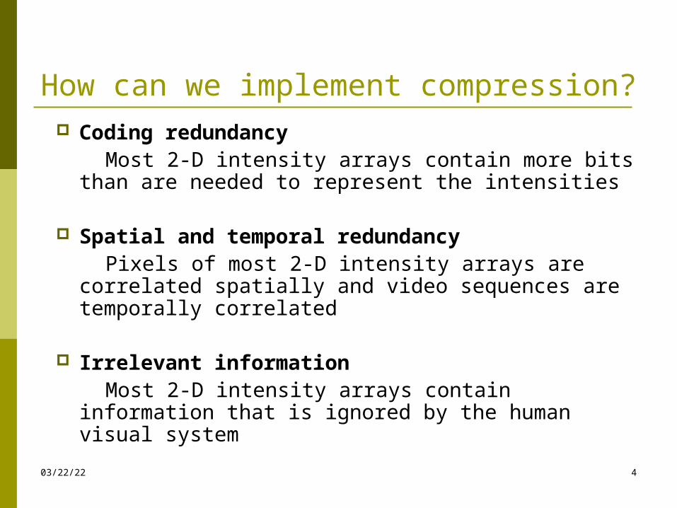
How can we implement compression? Coding redundancy Most 2-D intensity arrays contain more bits than

are needed to represent the intensities

Spatial and temporal redundancy Pixels of most 2-D intensity arrays are correlated

spatially and video sequences are temporally correlated

Irrelevant information Most 2-D intensity arrays contain information

that is ignored by the human visual system04/19/23 4

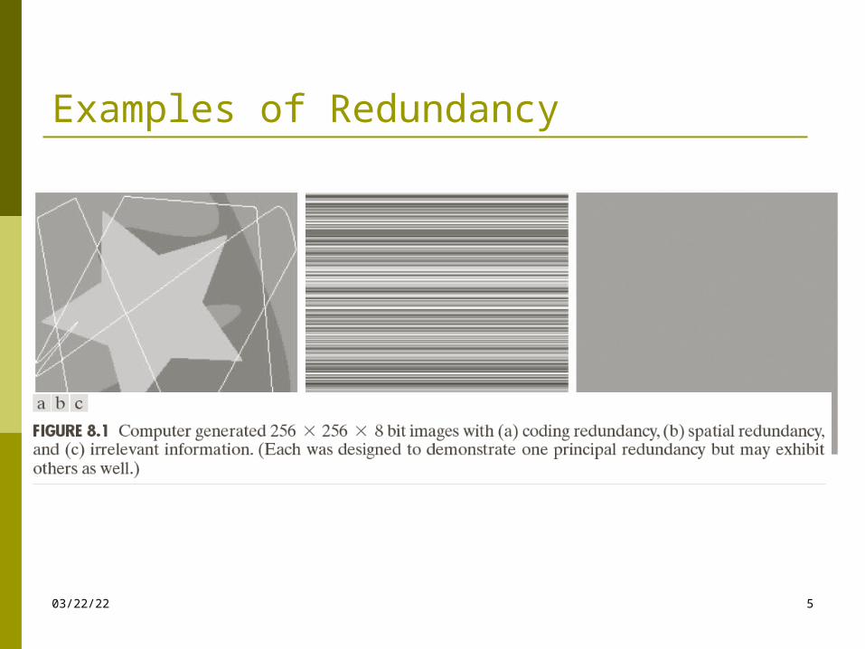
Examples of Redundancy

04/19/23 5

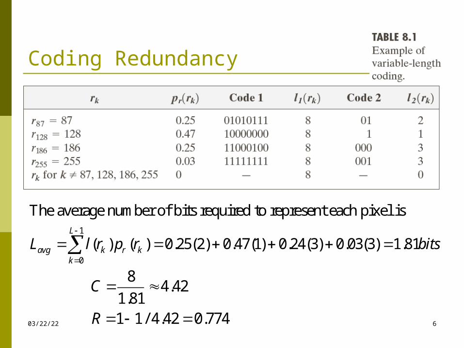
Coding Redundancy

04/19/23 6

1

0

The average number of bits required to represent each pixel is

( ) ( ) 0.25(2) 0.47(1) 0.24(3) 0.03(3) 1.81L

avg k r kk

L l r p r bits

8

4.421.811 1/ 4.42 0.774

C

R

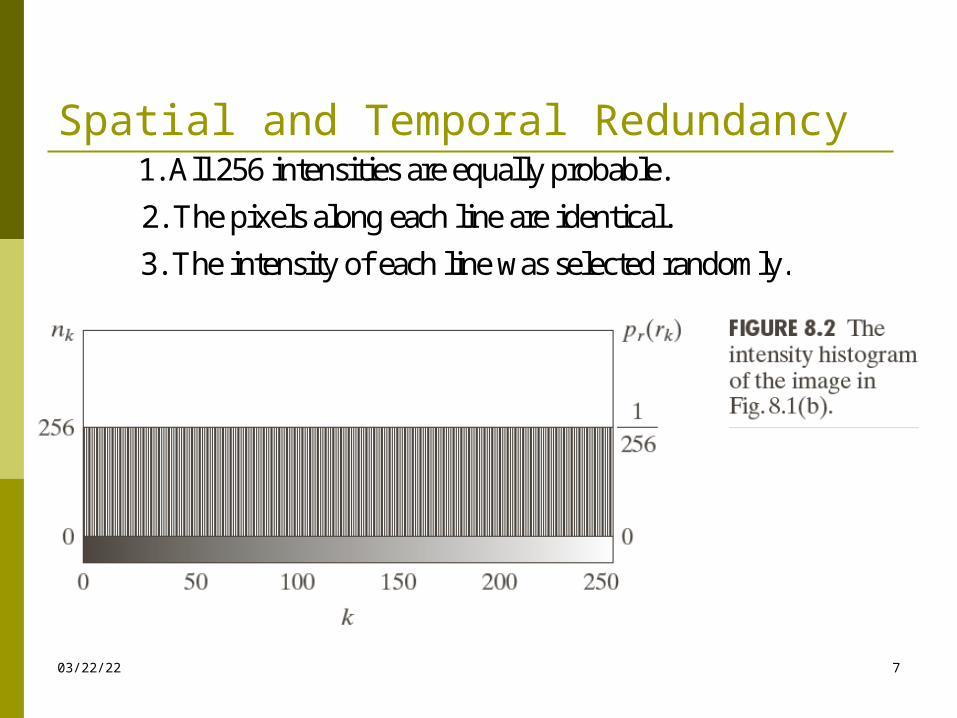
Spatial and Temporal Redundancy

04/19/23 7

1. All 256 intensities are equally probable.

2. The pixels along each line are identical.

3. The intensity of each line was selected randomly.

Spatial and Temporal Redundancy

04/19/23 8

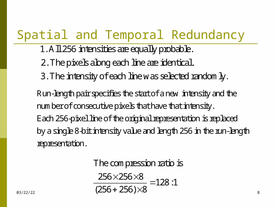
1. All 256 intensities are equally probable.

2. The pixels along each line are identical.

3. The intensity of each line was selected randomly.

Run-length pair specifies the start of a new intensity and the

number of consecutive pixels that have that intensity.

Each 256-pixel line of the original representation is replaced

by a single 8-bit intensity value and length 256 in the run-length

representation.

The compression ratio is

256 256 8128 :1

(256 256) 8

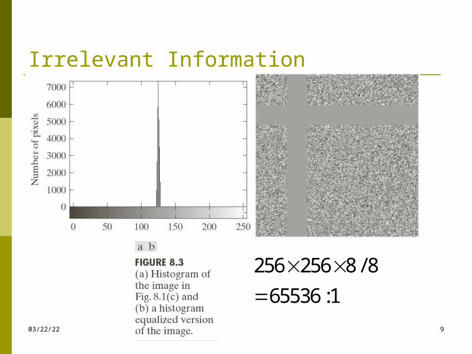
Irrelevant Information

04/19/23 9

256 256 8 / 8

65536 :1

Measuring Image Information

04/19/23 10

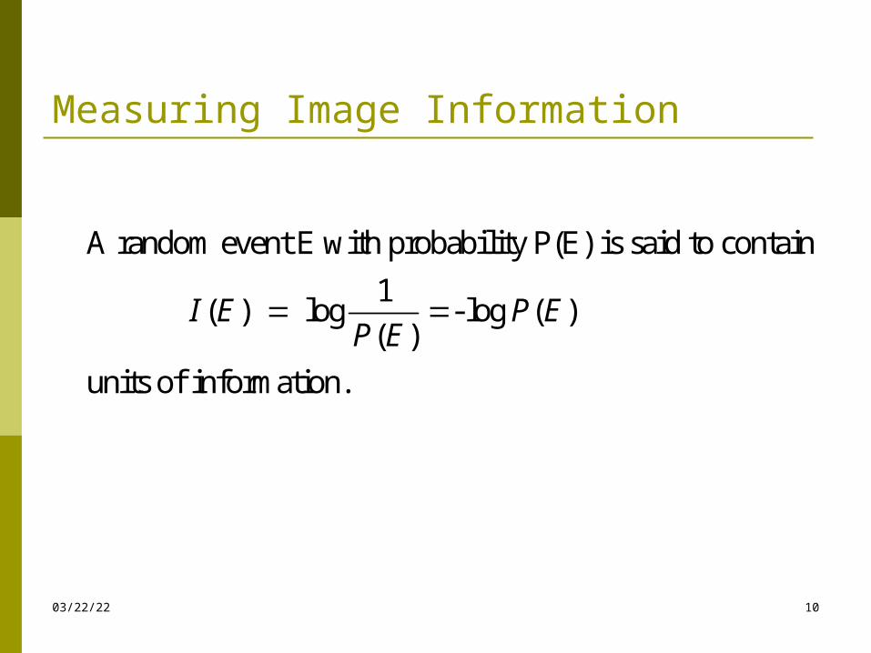
A random event E with probability P(E) is said to contain

1 ( ) log - log ( )

( )

units of information.

I E P EP E


1 2

1 2

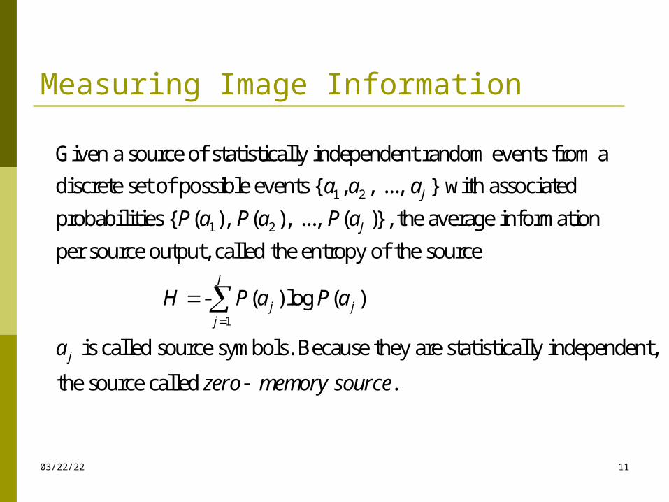
Given a source of statistically independent random events from a

discrete set of possible events { , , ..., } with associated

probabilities { ( ), ( ), ..., ( )}, the average information

per s

J

J

a a a

P a P a P a

1

ource output, called the entropy of the source

- ( ) log ( )

is called source symbols. Because they are statistically independent,

the source called .

J

j jj

j

H P a P a

a

zero memory source

04/19/23 11


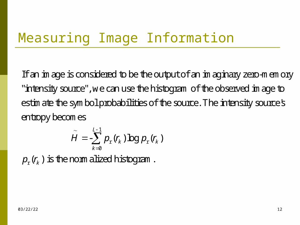
If an image is considered to be the output of an imaginary zero-memory

"intensity source", we can use the histogram of the observed image to

estimate the symbol probabilities of the source. The intensit

1

r r0

r

y source's

entropy becomes

- ( ) log ( )

( ) is the normalized histogram.

L

k kk

k

H p r p r

p r

04/19/23 12


2 2 2 2

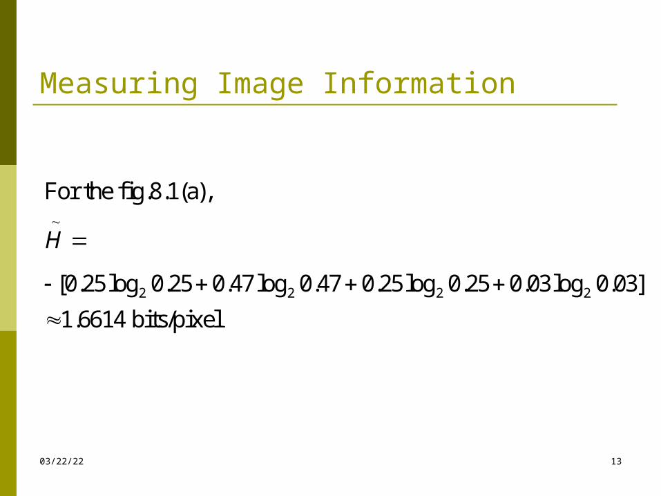
For the fig.8.1(a),

[0.25log 0.25 0.47 log 0.47 0.25log 0.25 0.03log 0.03]

1.6614 bits/pixel

H

04/19/23 13

Fidelity Criteria

1/221 1

0 0

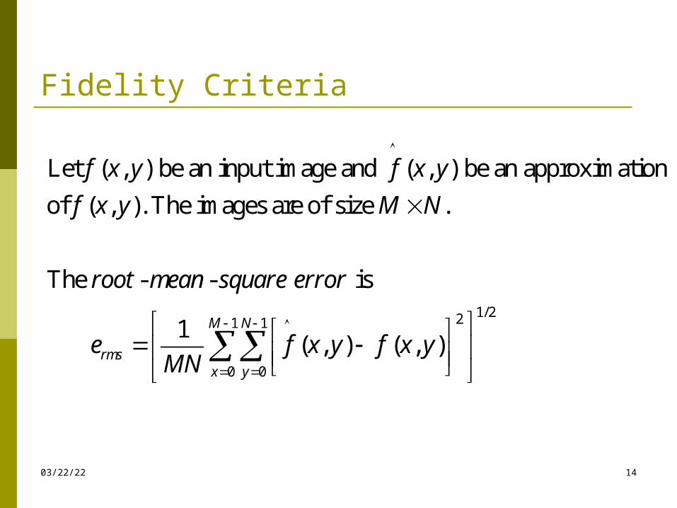
Let ( , ) be an input image and ( , ) be an approximation

of ( , ). The images are of size .

The - - is

1 ( , ) ( , )

M N

rmsx y

f x y f x y

f x y M N

root mean square error

e f x y f x yMN

04/19/23 14

Fidelity Criteria

ms

21 1

0 0ms 21 1

0 0

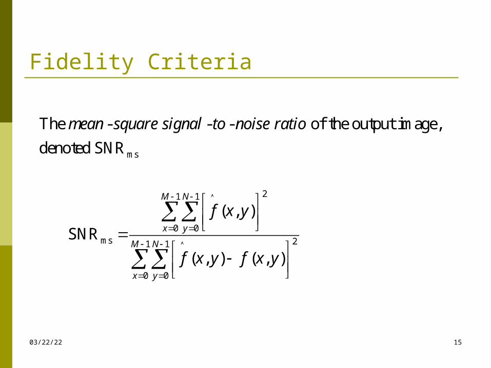
The - - - of the output image,

denoted SNR

( , )

SNR

( , ) ( , )

M N

x y

M N

x y

mean square signal to noise ratio

f x y

f x y f x y

04/19/23 15

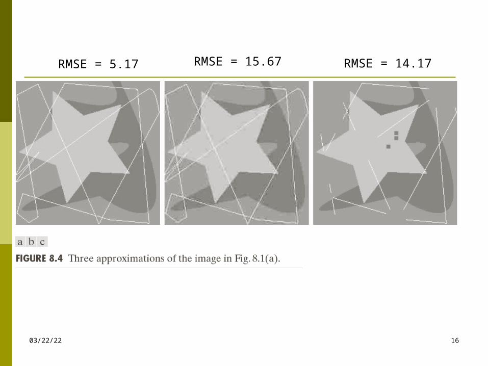
04/19/23 16

RMSE = 5.17 RMSE = 15.67 RMSE = 14.17

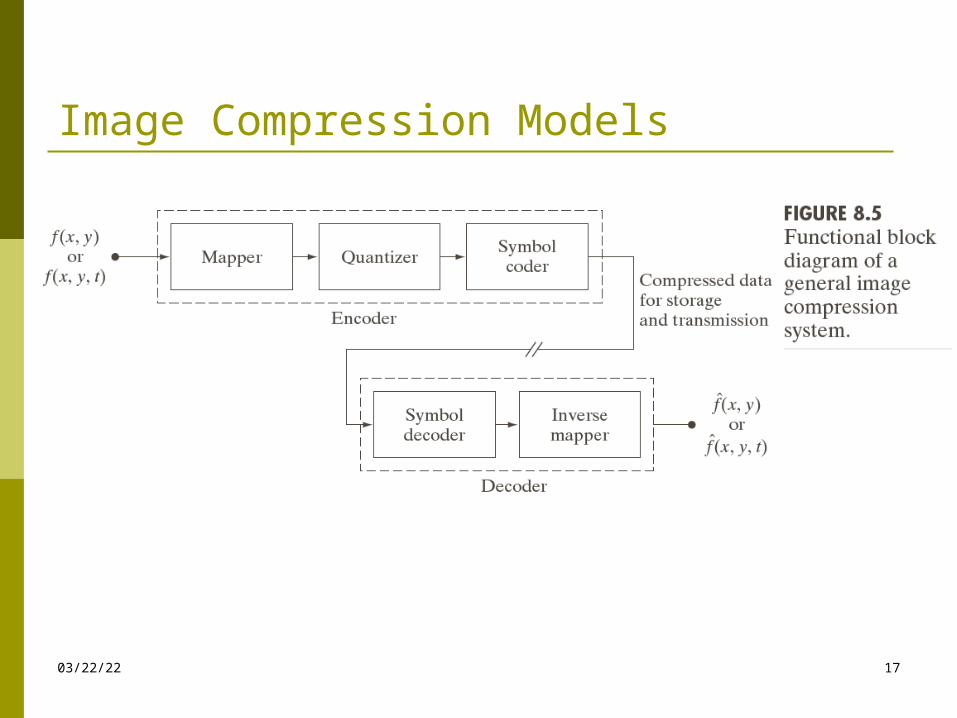
Image Compression Models

04/19/23 17

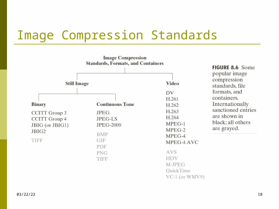
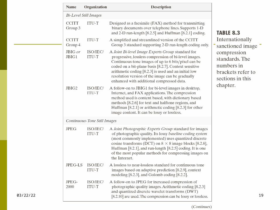
Image Compression Standards

04/19/23 18

04/19/23 19

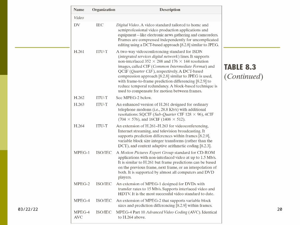
04/19/23 20

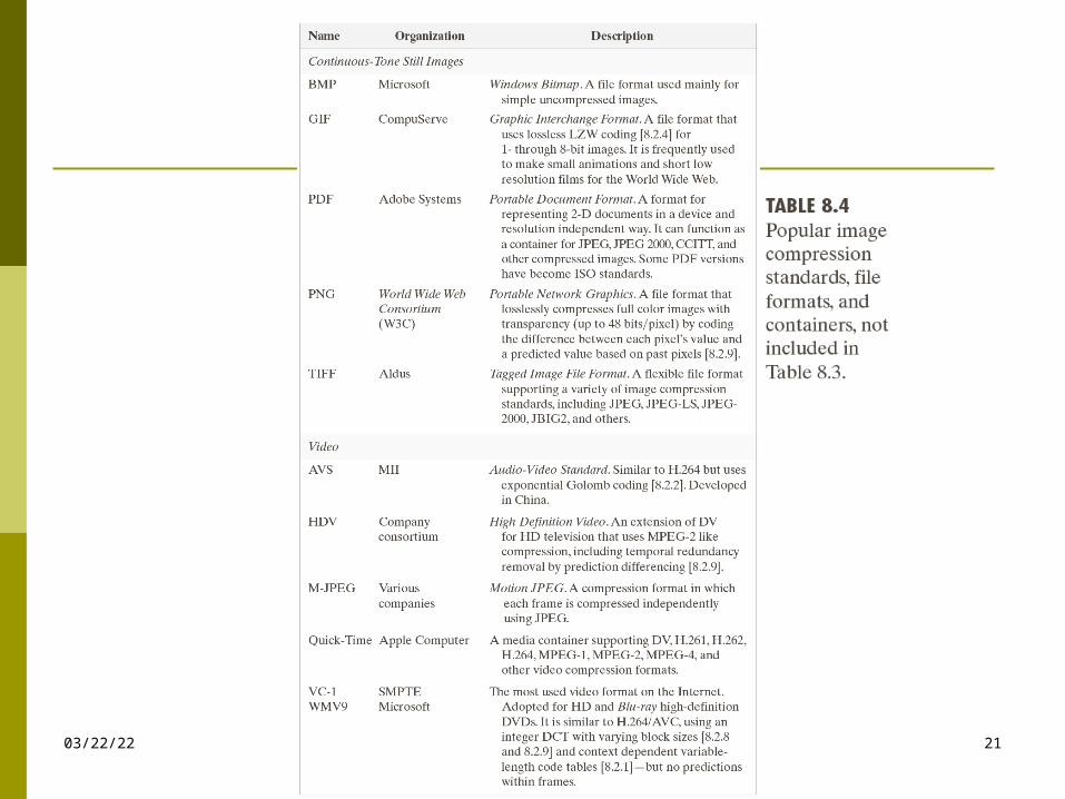
04/19/23 21

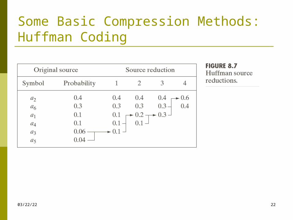
Some Basic Compression Methods:Huffman Coding

04/19/23 22

Some Basic Compression Methods:Huffman Coding

04/19/23 23

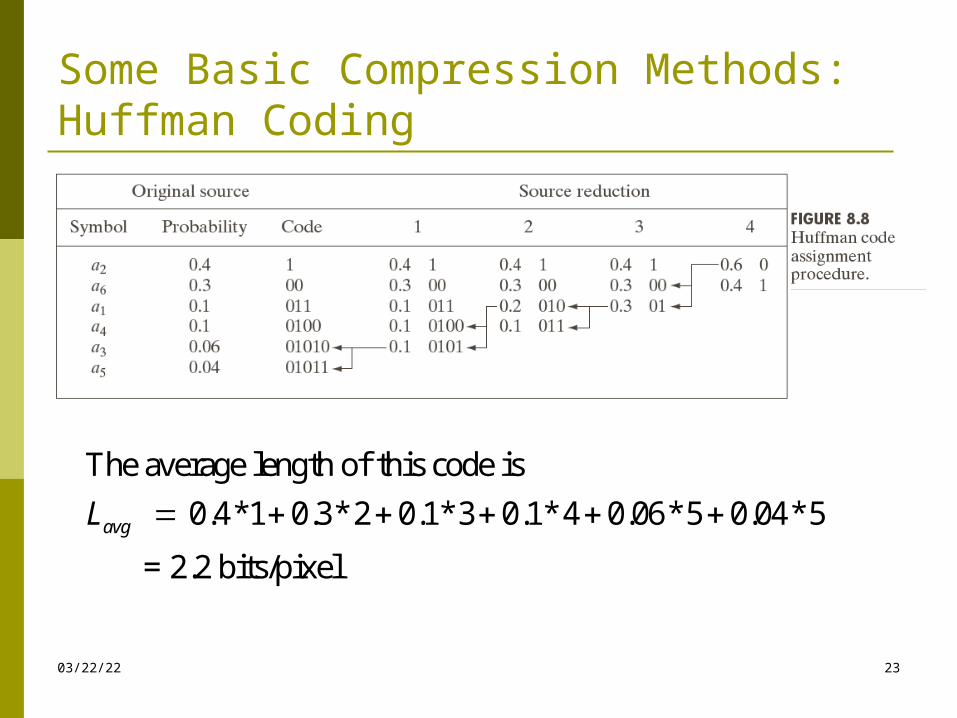
The average length of this code is

0.4*1 0.3*2 0.1*3 0.1*4 0.06*5 0.04*5

= 2.2 bits/pixel

avgL

Some Basic Compression Methods:Golomb Coding

04/19/23 24

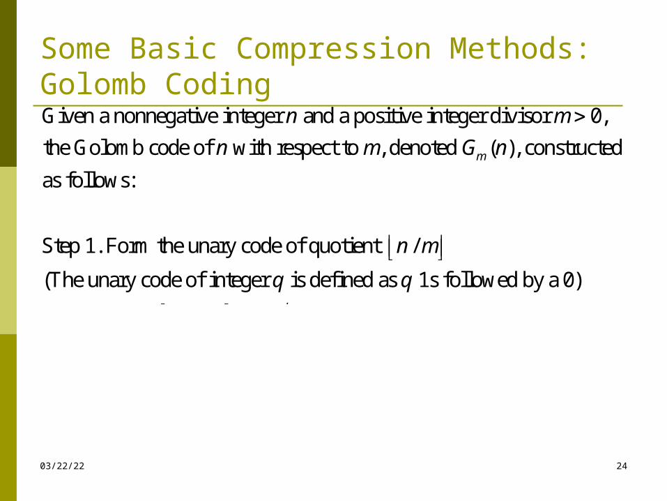
Given a nonnegative integer and a positive integer divisor 0,

the Golomb code of with respect to , denoted ( ), constructed

as follows:

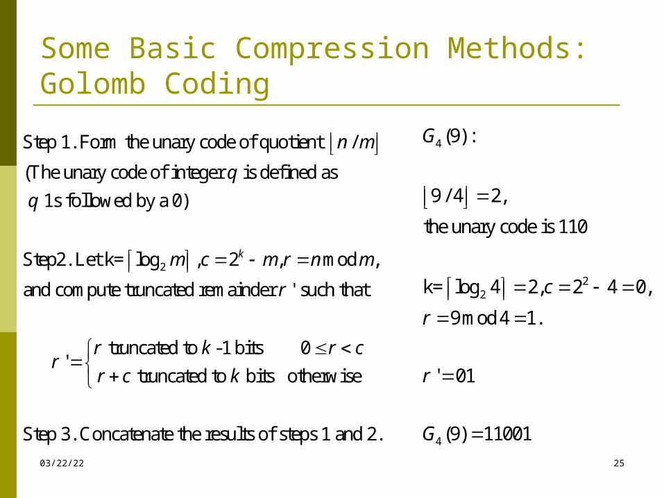
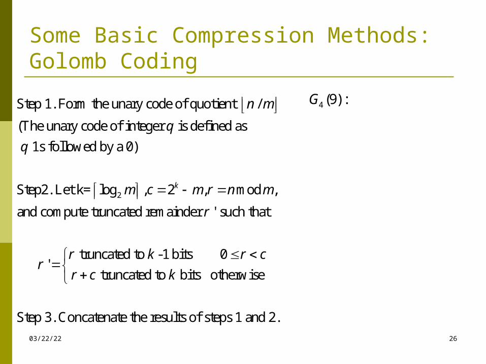
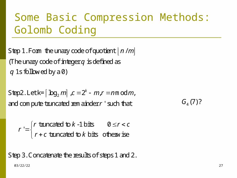
Step 1. Form the unary code of quotient /

(The unary

m

n m

n m G n

n m

2

code of integer is defined as 1s followed by a 0)

Step2. Let k= log , 2 , mod ,and compute truncated

remainder ' such that

truncated to -1 bits 0 '

trunca

k

q q

m c m r n m

r

r k r cr

r c

ted to bits otherwise

Step 3. Concatenate the results of steps 1 and 2.

k


04/19/23 25

2


(The unary code of integer is defined as

1s followed by a 0)

Step2. Let k= log , 2 , mod ,

and compute truncated remainder ' such that

k

n m

q

q

m c m r n m

r

r

truncated to -1 bits 0'

truncated to bits otherwise


r k r c

r c k

4

22

4

(9) :

9 / 4 2,

the unary code is 110

k= log 4 2, 2 4 0,

9mod 4 1.

' 01

(9) 11001

G

c

r

r

G


04/19/23 26

2



1s followed by a 0)



k

n m

q

q

m c m r n m

r

r




r k r c

r c k

4

22

4

(9) :

9 / 4 2,

the unary code is 110

k= log 4 2, 2 4 0,

9mod 4 1.

' 01

(9) 11001

G

c

r

r

G


04/19/23 27

2



1s followed by a 0)



k

n m

q

q

m c m r n m

r

r




r k r c

r c k

4 (7)?G

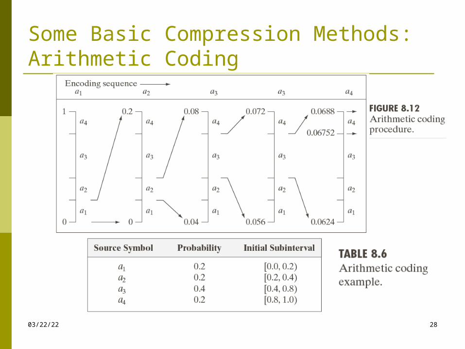
Some Basic Compression Methods:Arithmetic Coding

04/19/23 28

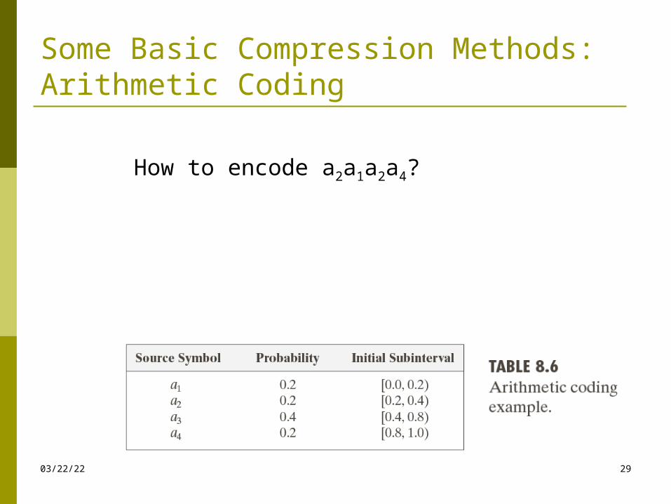
Some Basic Compression Methods:Arithmetic Coding

04/19/23 29

How to encode a2a1a2a4?

04/19/23 30

1.0

0.8

0.4

0.2

0.8

0.72

0.56

0.48

0.40.0

0.72

0.688

0.624

0.592

0.592

0.5856

0.5728

0.5664

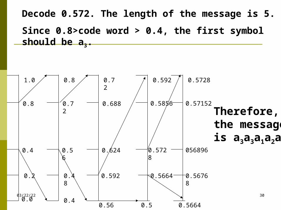
Therefore, the message is a3a3a1a2a4

0.5728

0.57152

056896

0.56768

Decode 0.572. The length of the message is 5.

Since 0.8>code word > 0.4, the first symbol should be a3.

0.56 0.56 0.5664

04/19/23 31

LZW (Dictionary coding)LZW (Dictionary coding)LZW (Dictionary coding)LZW (Dictionary coding)

LZW (Lempel-Ziv-Welch) coding, assigns fixed-length code words to variable length sequences of source symbols, but requires no a priori knowledge of the probability of the source symbols.

LZW is used in:

•Tagged Image file format (TIFF)

•Graphic interchange format (GIF)

•Portable document format (PDF)

LZW was formulated in 1984

04/19/23 32

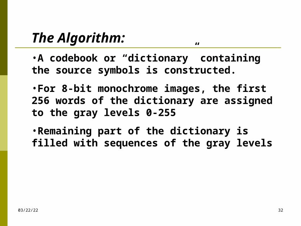
The Algorithm:•A codebook or “dictionary” containing the source symbols is constructed.

•For 8-bit monochrome images, the first 256 words of the dictionary are assigned to the gray levels 0-255

•Remaining part of the dictionary is filled with sequences of the gray levels

04/19/23 33

Important features of LZWImportant features of LZW

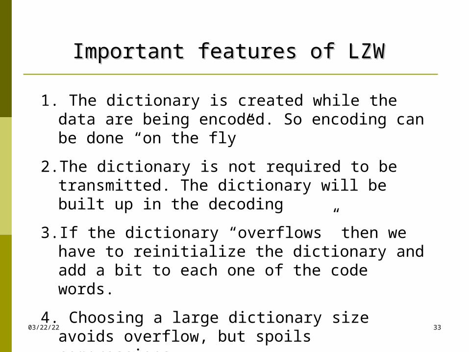
1. The dictionary is created while the data are being encoded. So encoding can be done “on the fly”

2. The dictionary is not required to be transmitted. The dictionary will be built up in the decoding

3. If the dictionary “overflows” then we have to reinitialize the dictionary and add a bit to each one of the code words.

4. Choosing a large dictionary size avoids overflow, but spoils compressions

04/19/23 34

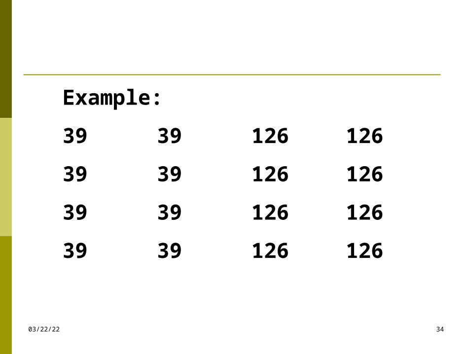
Example:

39 39 126 126

39 39 126 126

39 39 126 126

39 39 126 126

04/19/23 35

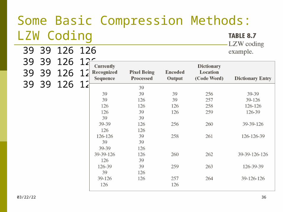
Some Basic Compression Methods:LZW Coding

04/19/23 36

39 39 126 12639 39 126 12639 39 126 12639 39 126 126

04/19/23 37

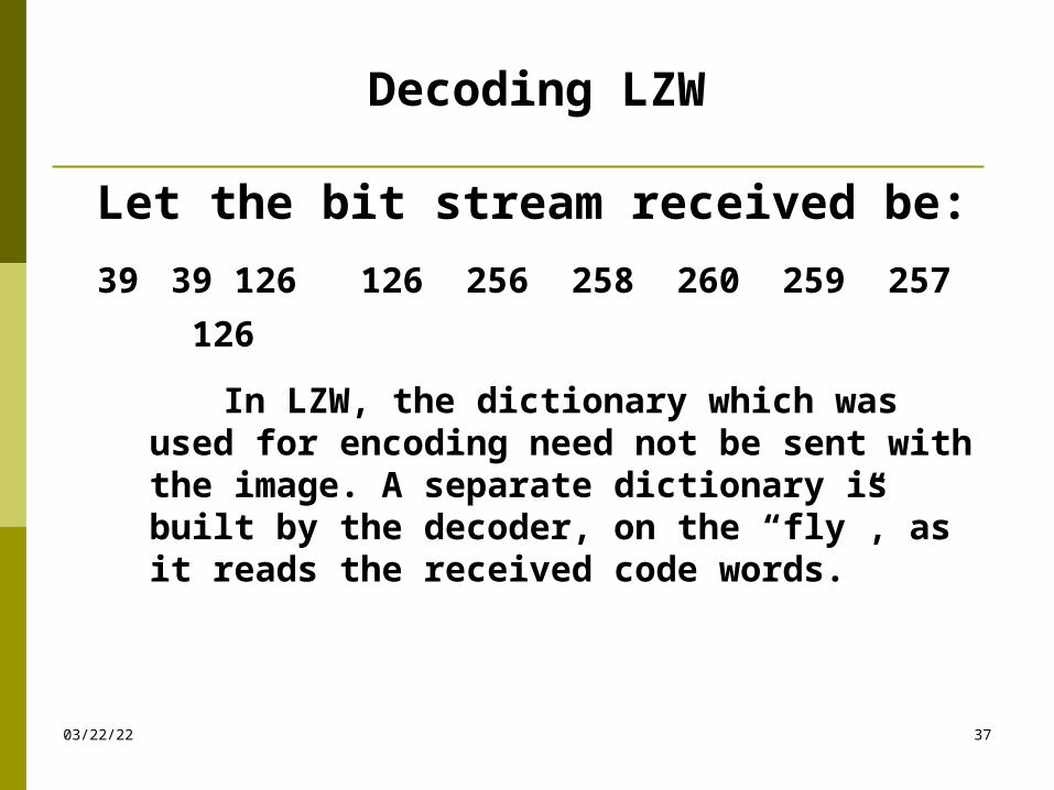
Let the bit stream received be:

39 39 126 126 256 258 260 259 257

126

In LZW, the dictionary which was used for encoding need not be sent with the image. A separate dictionary is built by the decoder, on the “fly”, as it reads the received code words.

Decoding LZW

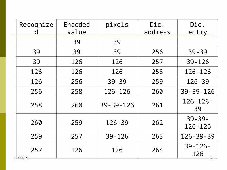
04/19/23 38

Recognized

Encoded value

pixels Dic. address

Dic. entry

39 39

39 39 39 256 39-39

39 126 126 257 39-126

126 126 126 258 126-126

126 256 39-39 259 126-39

256 258 126-126 260 39-39-126

258 260 39-39-126 261126-126-

39

260 259 126-39 26239-39-126-

126

259 257 39-126 263 126-39-39

257 126 126 26439-126-

126

Some Basic Compression Methods:Run-Length Coding

04/19/23 39

1. Run-length Encoding, or RLE is a technique used to reduce the size of a repeating string of characters.

2. This repeating string is called a run, typically RLE encodes a run of symbols into two bytes , a count and a symbol.

3. RLE can compress any type of data

4. RLE cannot achieve high compression ratios compared to other compression methods


04/19/23 40

5. It is easy to implement and is quick to execute.

6. Run-length encoding is supported by most bitmap file formats such as TIFF, BMP and PCX


04/19/23 41

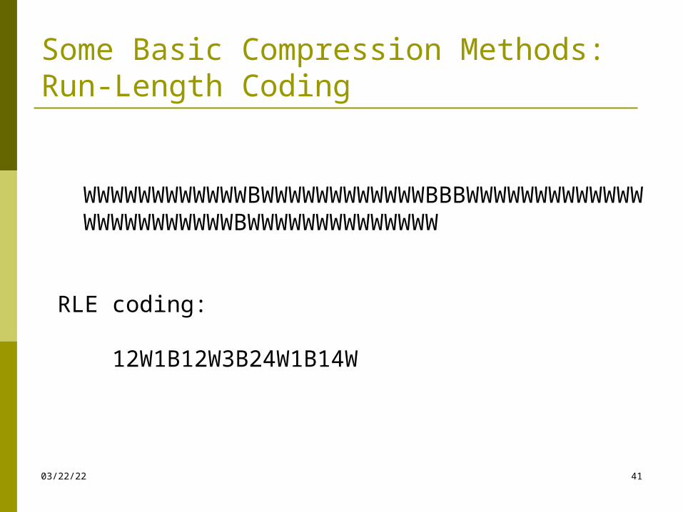
WWWWWWWWWWWWBWWWWWWWWWWWWBBBWWWWWWWWWWWWWWWWWWWWWWWWBWWWWWWWWWWWWWW

RLE coding:

12W1B12W3B24W1B14W

Some Basic Compression Methods:Symbol-Based Coding

04/19/23 42

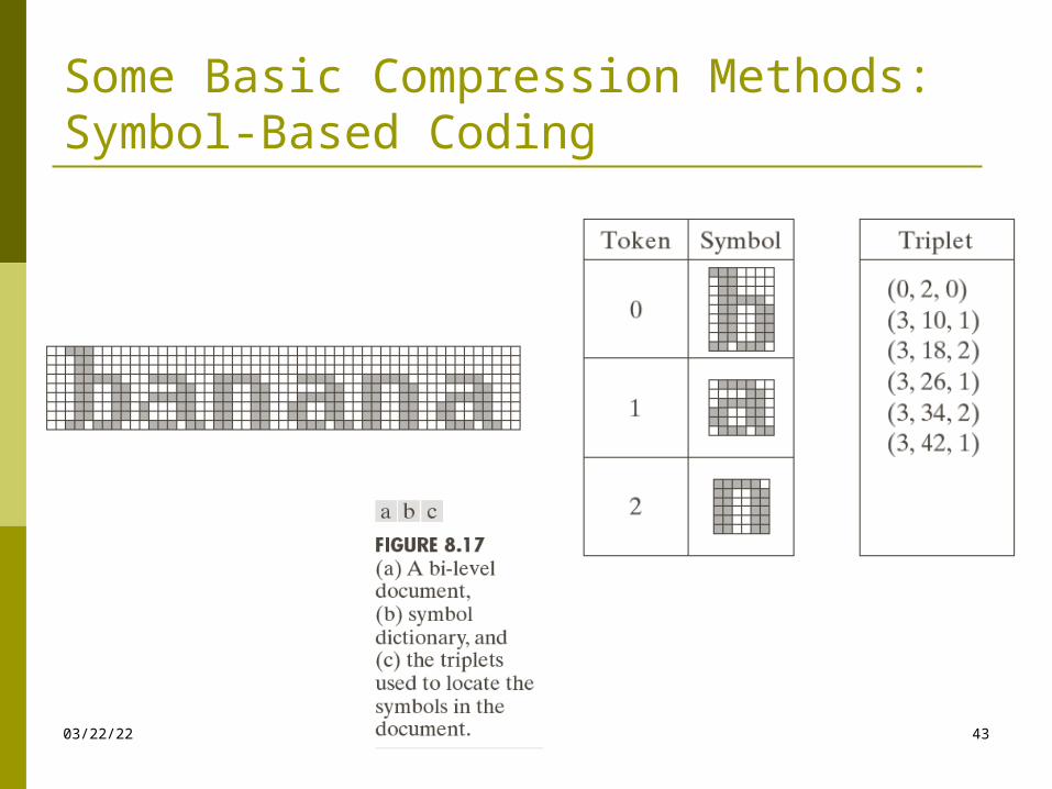
In symbol- or token-based coding, an image is represented as a collection of frequently occurring

sub-images, called symbols.

Each symbol is stored in a symbol dictionary

Image is coded as a set of triplets

{(x1,y1,t1), (x2, y2, t2), …}

Some Basic Compression Methods:Symbol-Based Coding

04/19/23 43

Some Basic Compression Methods:Bit-Plane Coding

04/19/23 44

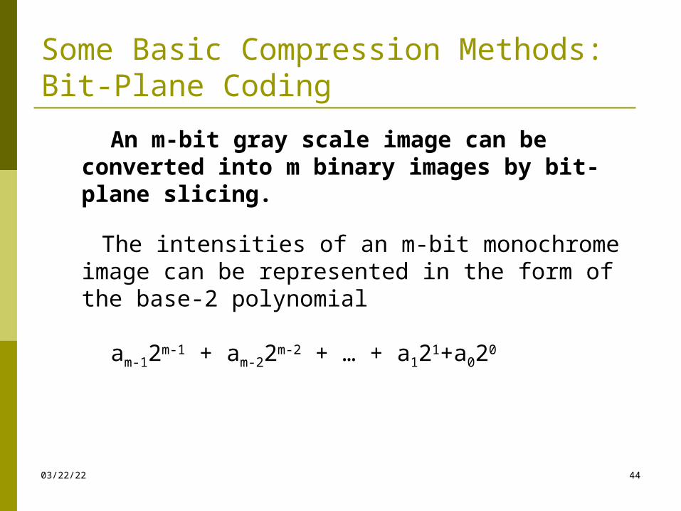
An m-bit gray scale image can be converted into m binary images by bit-plane slicing.

The intensities of an m-bit monochrome image can be represented in the form of the base-2 polynomial

am-12m-1 + am-22m-2 + … + a121+a020


04/19/23 45

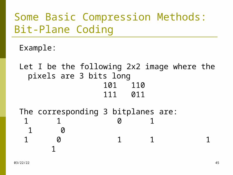
Example:

Let I be the following 2x2 image where the pixels are 3 bits long

101 110 111 011

The corresponding 3 bitplanes are: 1 1 0 1 1 0 1 0 1 1 1 1


04/19/23 46

An m-bit gray scale image can be converted into m binary images by bit-plane slicing.

These individual images are then encoded using run-length coding.

― Code the bit-planes separately, using RLE (flatten each plane row-wise into a 1D array), Golomb coding, or any other lossless compression technique.

04/19/23 47

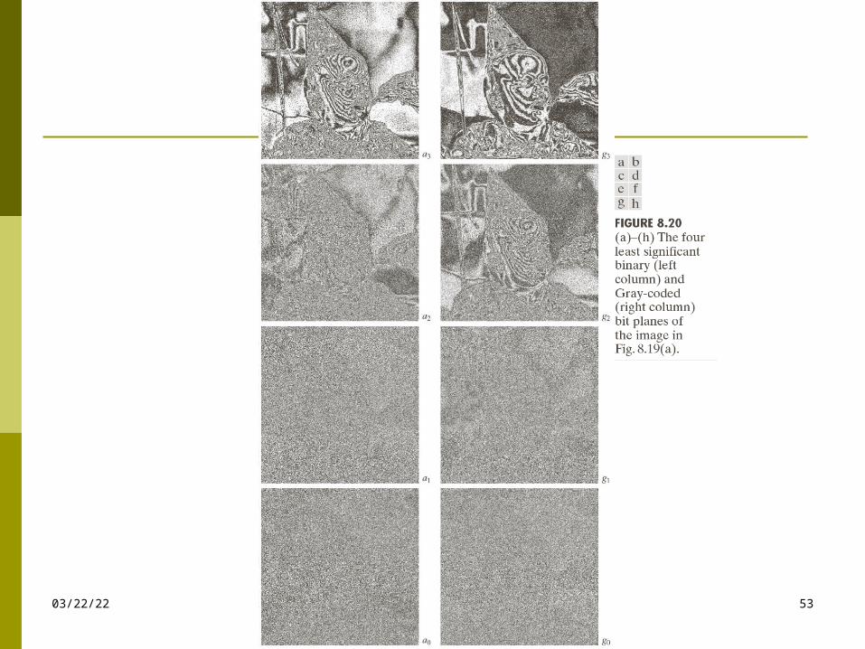
However, a small difference in the gray level of adjacent pixels can cause a disruption of the run of zeroes or ones.

Eg: Let us say one pixel has a gray level of 127 and the next pixel has a gray level of 128.

In binary:

127 = 01111111 & 128 = 10000000

Therefore a small change in gray level has decreased the run-lengths in all the bit-planes!

A Problem in Bit-Plane Slicing

04/19/23 48

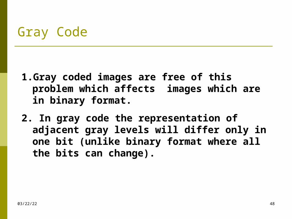
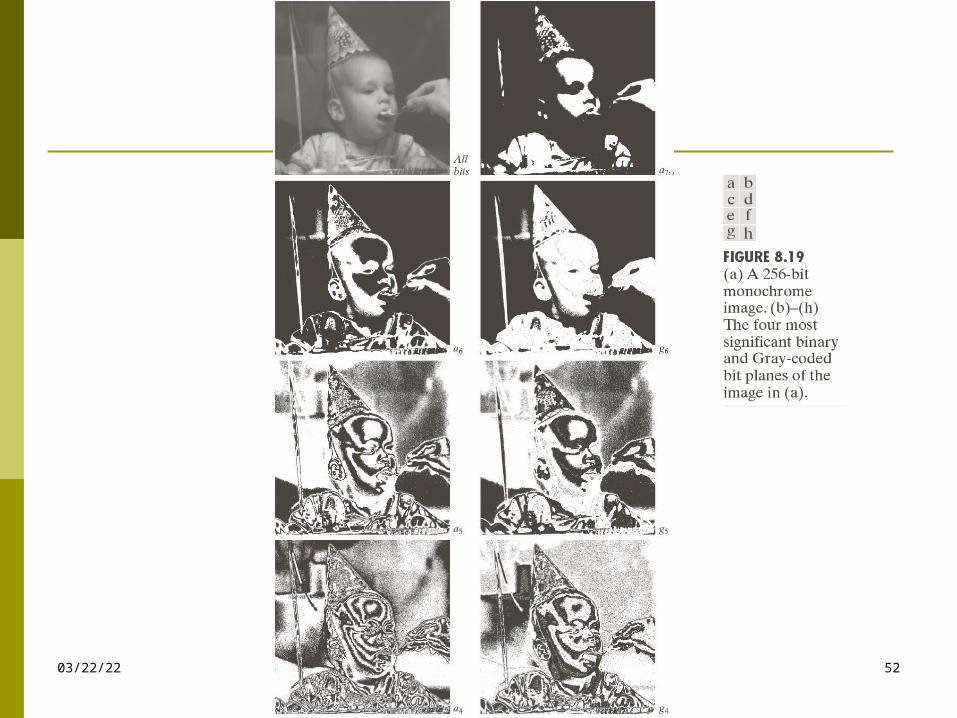
1. Gray coded images are free of this problem which affects images which are in binary format.

2. In gray code the representation of adjacent gray levels will differ only in one bit (unlike binary format where all the bits can change).

Gray Code

04/19/23 49

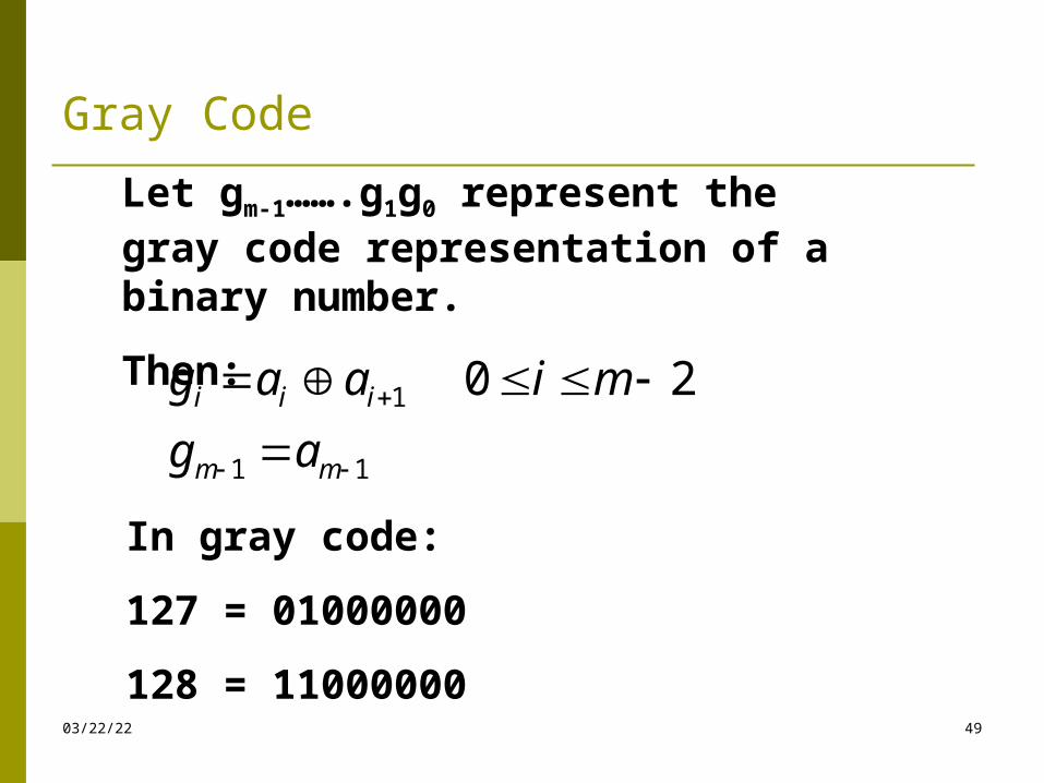
Let gm-1…….g1g0 represent the gray code representation of a binary number.

Then:

11

1 20

mm

iii

ag

miaag

In gray code:

127 = 01000000

128 = 11000000

Gray Code

Gray Coding

04/19/23 50

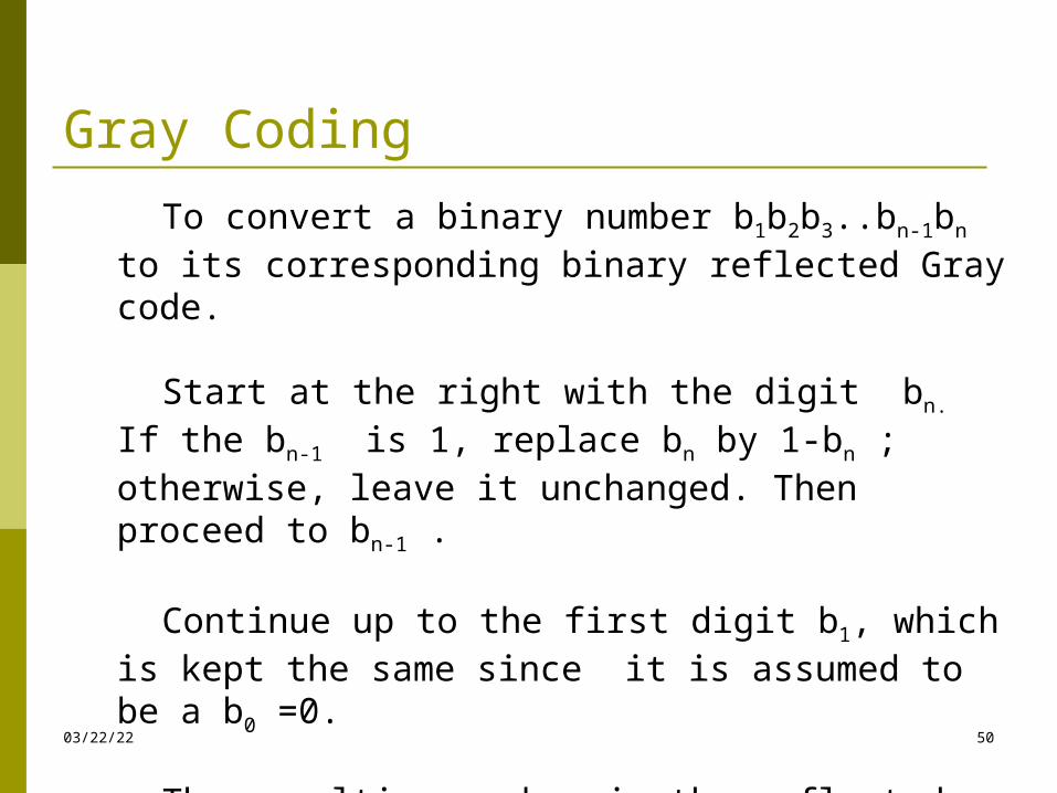
To convert a binary number b1b2b3..bn-1bn to its corresponding binary reflected Gray code.

Start at the right with the digit bn. If the bn-1 is 1, replace bn by 1-bn ; otherwise, leave it unchanged. Then proceed to bn-1 .

Continue up to the first digit b1, which is kept the same since it is assumed to be a b0 =0.

The resulting number is the reflected binary Gray code.

Examples: Gray Coding

04/19/23 51

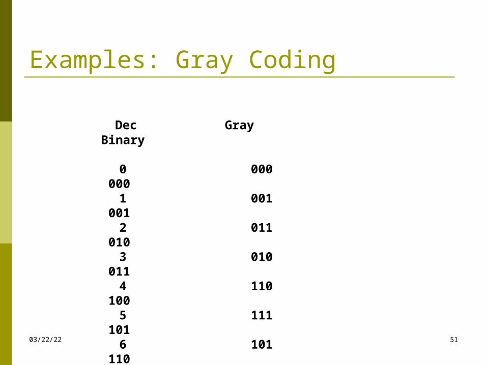
Dec Gray Binary 0 000 000 1 001 001 2 011 010 3 010 011 4 110 100 5 111 101 6 101 110 7 100 111

04/19/23 52

04/19/23 53

04/19/23 54

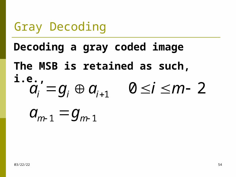
Decoding a gray coded image

The MSB is retained as such, i.e.,

11

1 20

mm

iii

ga

miaga

Gray Decoding

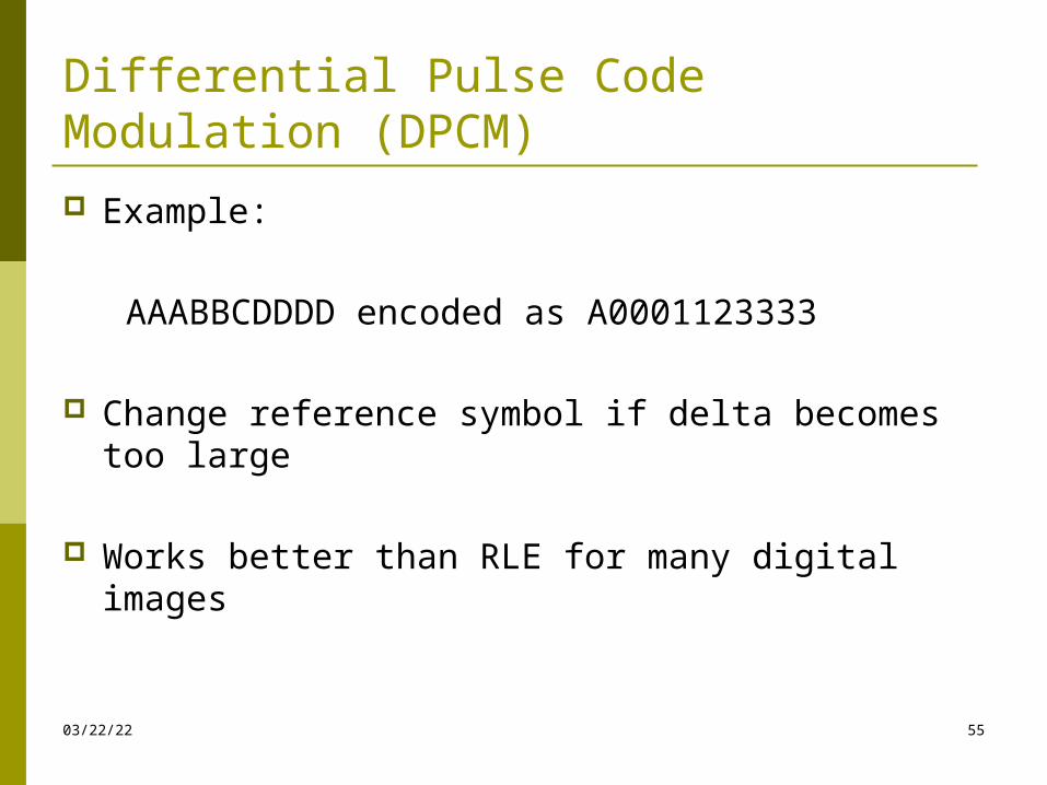
Differential Pulse Code Modulation (DPCM)

Example:

AAABBCDDDD encoded as A0001123333

Change reference symbol if delta becomes too large

Works better than RLE for many digital images

04/19/23 55

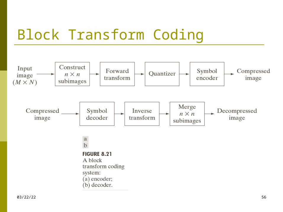
Block Transform Coding

04/19/23 56


04/19/23 57

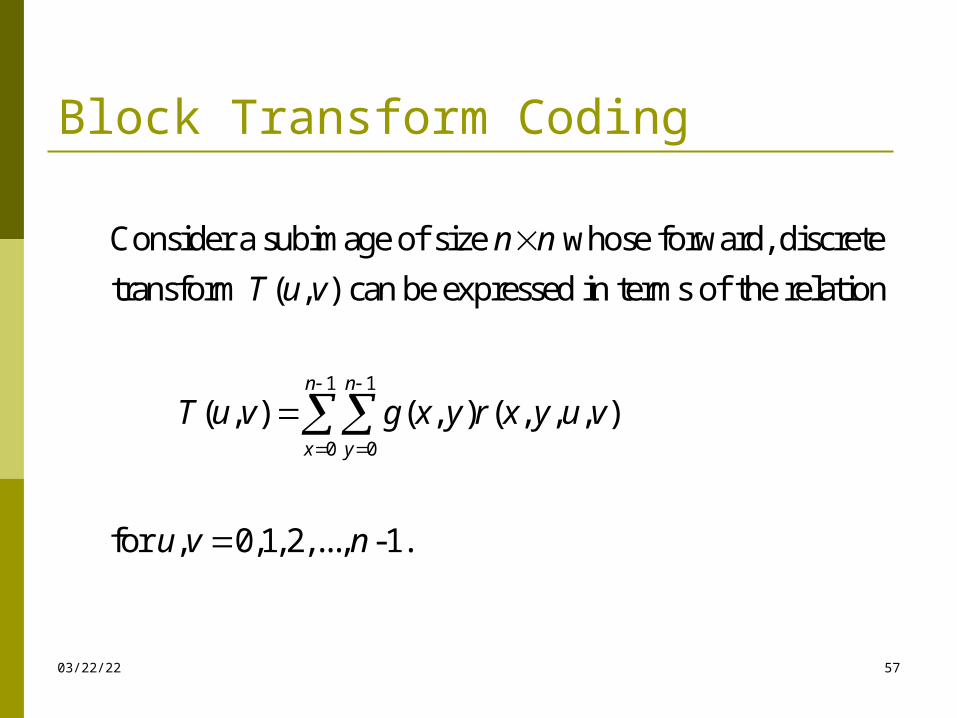
1 1

0 0

Consider a subimage of size whose forward, discrete

transform ( , ) can be expressed in terms of the relation

( , ) ( , ) ( , , , )

for , 0,1, 2,..., -1.

n n

x y

n n

T u v

T u v g x y r x y u v

u v n


04/19/23 58

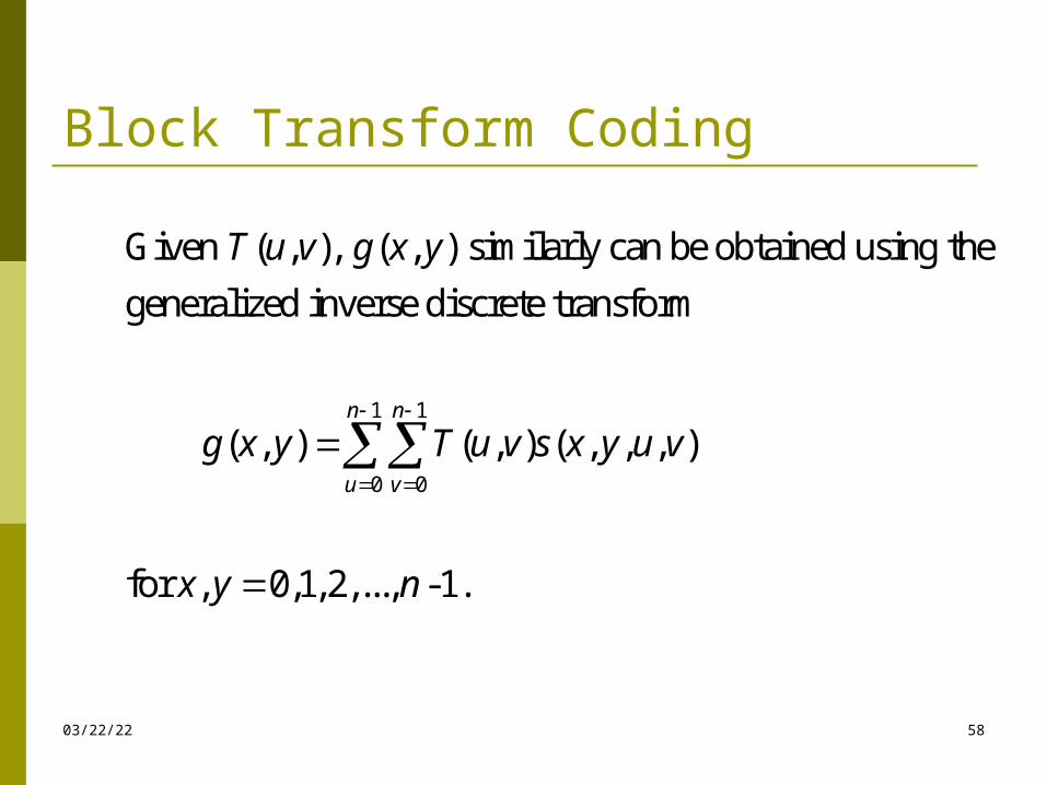
1 1

0 0

Given ( , ), ( , ) similarly can be obtained using the

generalized inverse discrete transform

( , ) ( , ) ( , , , )

for , 0,1, 2,..., -1.

n n

u v

T u v g x y

g x y T u v s x y u v

x y n

04/19/23 59

Image transform Two main types:

-Orthogonal transform:

e.g. Walsh-Hadamard transform, DCT

-Subband transform:

e.g. Wavelet transform

04/19/23 60

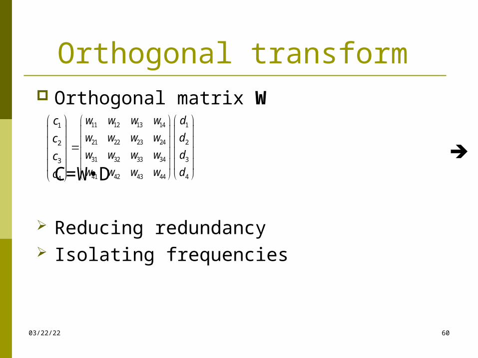
Orthogonal transform Orthogonal matrix W

C=W•D

Reducing redundancy Isolating frequencies

11 12 13 14

21 22 23 24

31 32 33 34

41 42 43 44

w w w w

w w w w

w w w w

w w w w

1

2

3

4

c

c

c

c

1

2

3

4

d

d

d

d

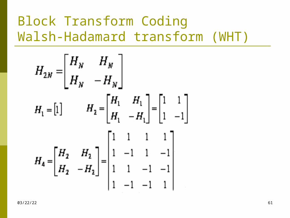
Block Transform CodingWalsh-Hadamard transform (WHT)

04/19/23 61

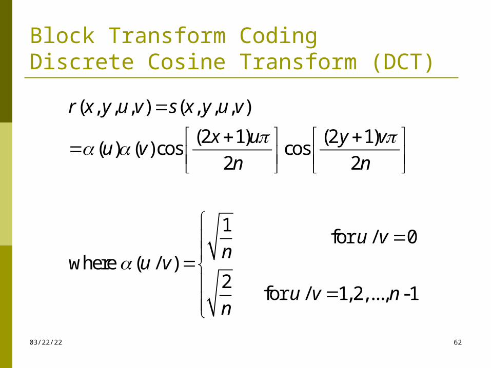
Block Transform CodingDiscrete Cosine Transform (DCT)

04/19/23 62

( , , , ) ( , , , )

(2 1) (2 1)( ) ( ) cos cos

2 2

1 for / 0

where ( / )2

for / 1, 2,..., -1

r x y u v s x y u v

x u y vu v

n n

u vn

u v

u v nn

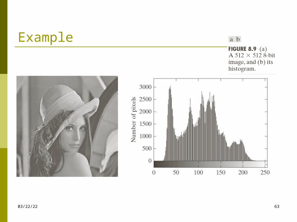
Example

04/19/23 63

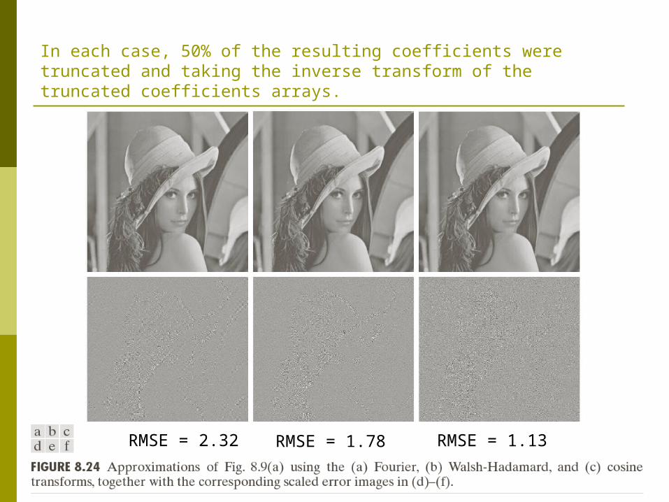
In each case, 50% of the resulting coefficients were truncated and taking the inverse transform of the truncated coefficients arrays.

04/19/23 64

RMSE = 2.32 RMSE = 1.78 RMSE = 1.13

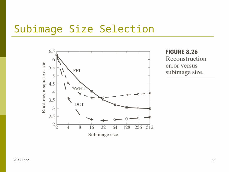
Subimage Size Selection

04/19/23 65

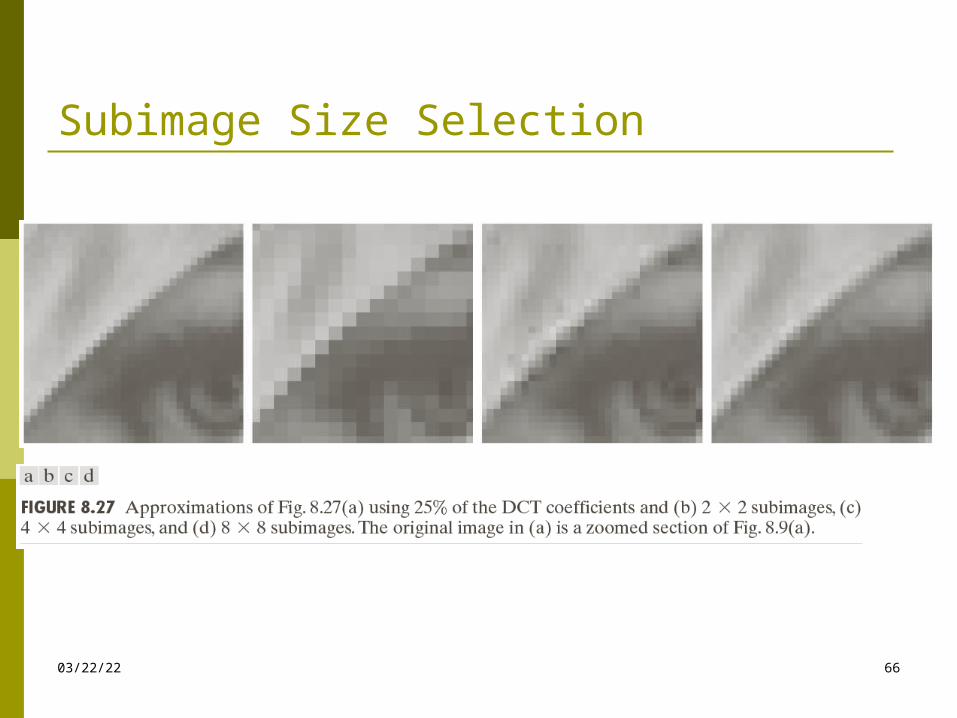
Subimage Size Selection

04/19/23 66

Bit Allocation

04/19/23 67

The overall process of truncating, quantizing, and coding the coefficients of a transformed subimage is commonly called bit allocation

Zonal coding The retained coefficients are selected on the basis of

maximum variance

Threshold coding The retained coefficients are selected on the basis of

maximum magnitude

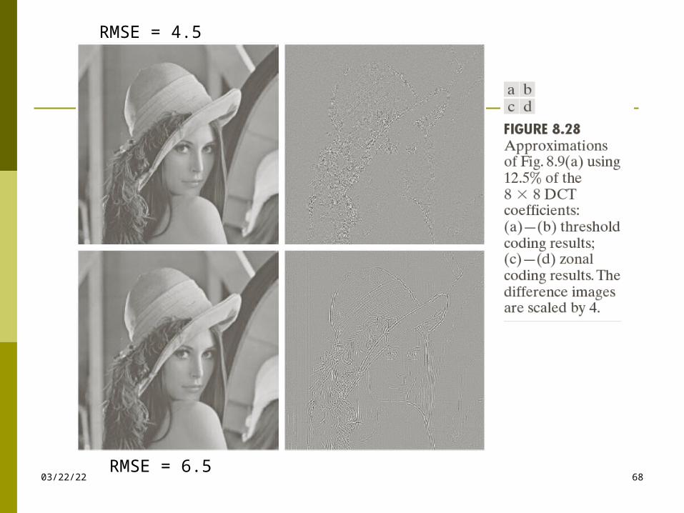
04/19/23 68RMSE = 6.5

RMSE = 4.5

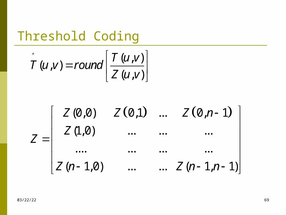
Threshold Coding

04/19/23 69

( , )( , )

( , )

(0,0) 0,1 ... 0, 1

(1,0) ... ... ...

.... ... ... ...

( 1,0) ... ... ( 1, 1)

T u vT u v round

Z u v

Z Z Z n

ZZ

Z n Z n n

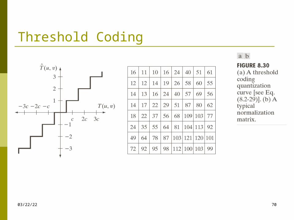
Threshold Coding

04/19/23 70

Threshold Coding

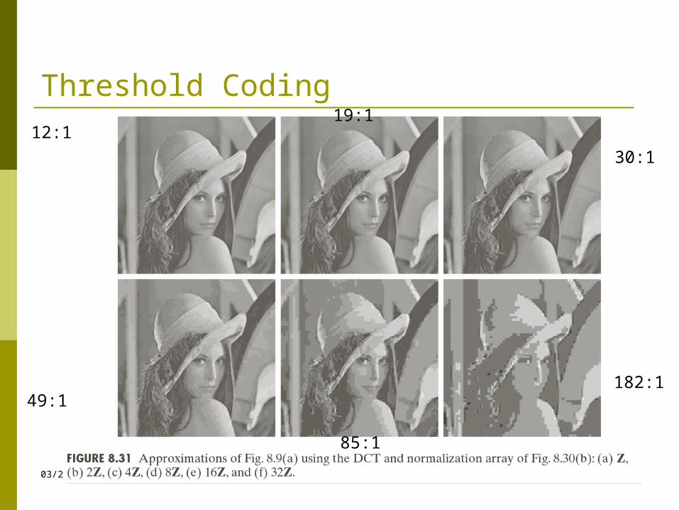
04/19/23 71

12:1

30:1

19:1

85:1

49:1182:1

Fact about JPEG Compression

JPEG stands for Joint Photographic Experts Group

Used on 24-bit color files.

Works well on photographic images.

Although it is a lossy compression technique, it yields an excellent quality image with high compression rates.

04/19/23 72

Fact about JPEG Compression

It defines three different coding systems:

1. a lossy baseline coding system, adequate for most compression applications

2. an extended coding system for greater compression, higher precision, or progressive reconstruction applications

3. A lossless independent coding system for reversible compression

04/19/23 73

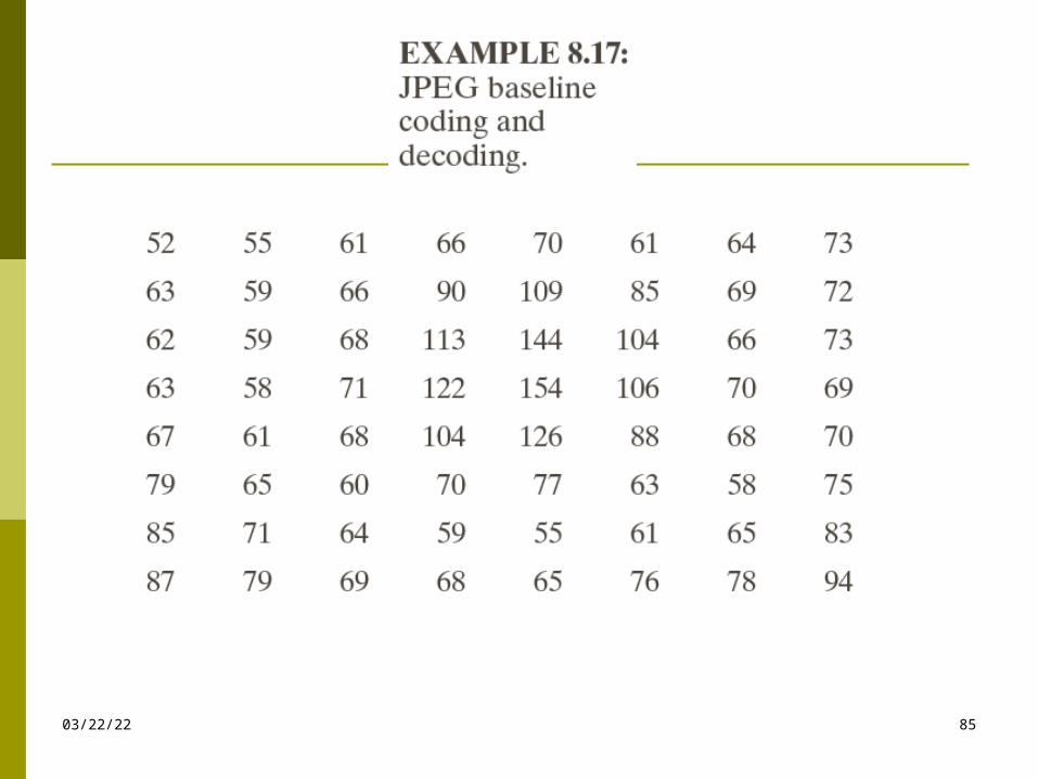
Steps in JPEG Compression

1. (Optionally) If the color is represented in RGB mode, translate it to YUV.

2. Divide the file into 8 X 8 blocks.

3. Transform the pixel information from the spatial domain to the frequency domain with the Discrete Cosine Transform.

4. Quantize the resulting values by dividing each coefficient by an integer value and rounding off to the nearest integer.

5. Look at the resulting coefficients in a zigzag order. Do a run-length encoding of the coefficients ordered in this manner, followed by Huffman coding.

04/19/23 74

Step 1a: Converting RGB to YUV

YUV color mode stores color in terms of its luminance (brightness) and chrominance (hue).

The human eye is less sensitive to chrominance than luminance.

YUV is not required for JPEG compression, but it gives a better compression rate.

04/19/23 75

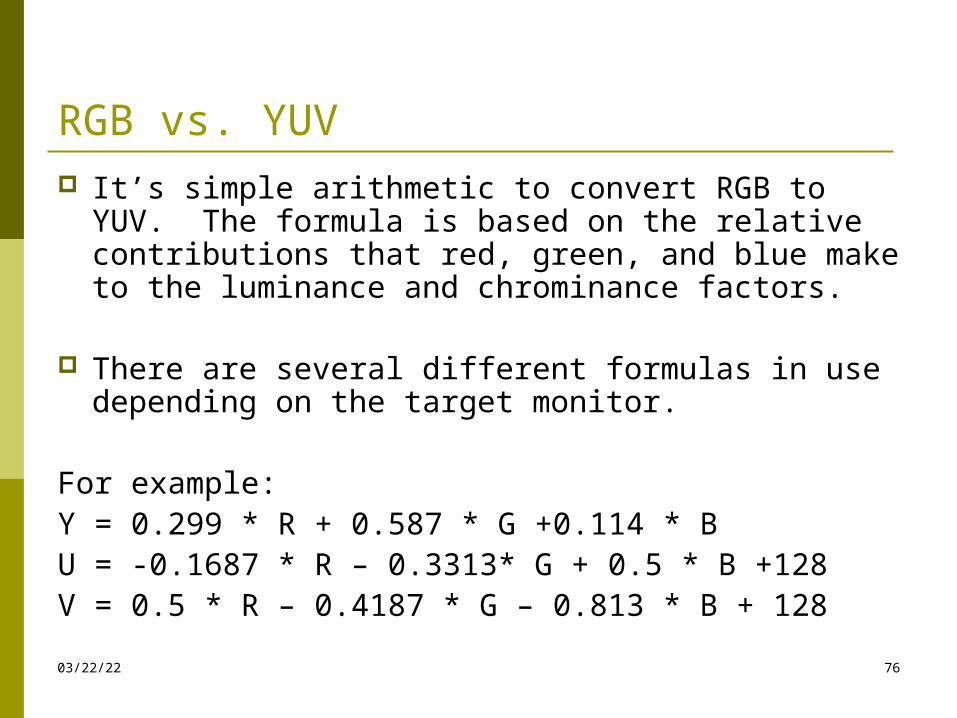
RGB vs. YUV It’s simple arithmetic to convert RGB to YUV. The

formula is based on the relative contributions that red, green, and blue make to the luminance and chrominance factors.

There are several different formulas in use depending on the target monitor.

For example:Y = 0.299 * R + 0.587 * G +0.114 * BU = -0.1687 * R – 0.3313* G + 0.5 * B +128V = 0.5 * R – 0.4187 * G – 0.813 * B + 12804/19/23 76

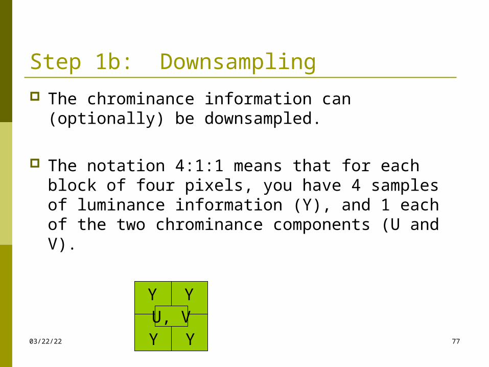
Step 1b: Downsampling

The chrominance information can (optionally) be downsampled.

The notation 4:1:1 means that for each block of four pixels, you have 4 samples of luminance information (Y), and 1 each of the two chrominance components (U and V).

04/19/23 77

Y Y

Y YU, V

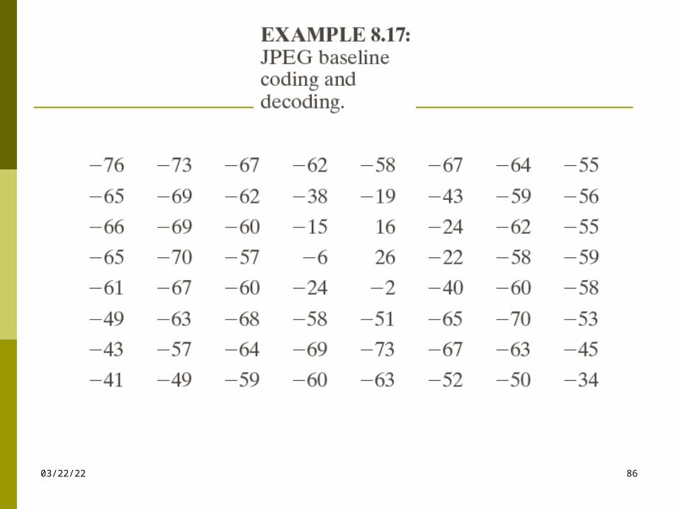
Step 2: Divide into 8 X 8 blocks If the file doesn’t divide evenly into 8 X 8 blocks,

extra pixels are added to the end and discarded after the compression.

The values are shifted “left” by subtracting 128.

04/19/23 78

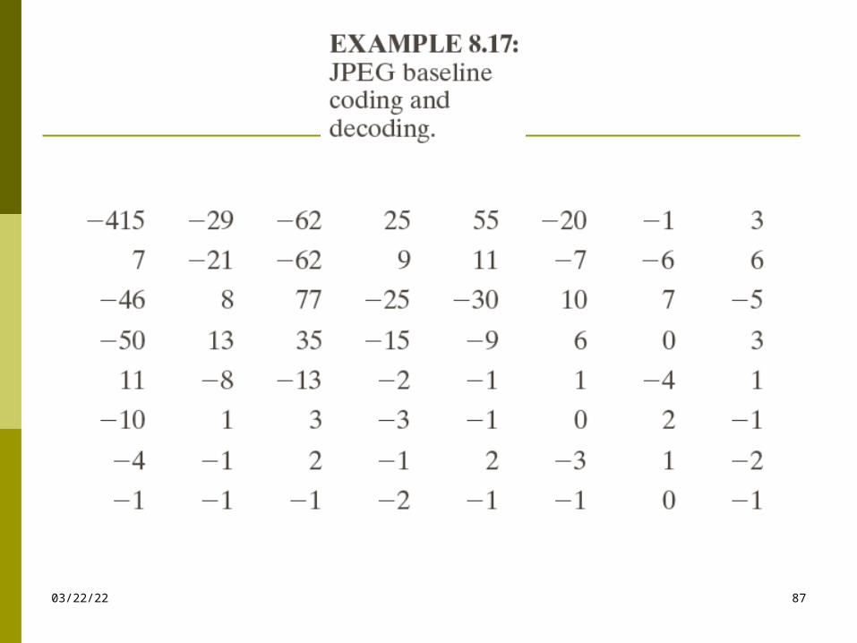
Discrete Cosine Transform

The DCT transforms the data from the spatial domain to the frequency domain.

The spatial domain shows the amplitude of the color as you move through space

The frequency domain shows how quickly the amplitude of the color is changing from one pixel to the next in an image file.

04/19/23 79

Step 3: DCT The frequency domain is a better representation

for the data because it makes it possible for you to separate out – and throw away – information that isn’t very important to human perception.

The human eye is not very sensitive to high frequency changes – especially in photographic images, so the high frequency data can, to some extent, be discarded.

04/19/23 80

Step 3: DCT

The color amplitude information can be thought of as a wave (in two dimensions).

You’re decomposing the wave into its component frequencies.

For the 8 X 8 matrix of color data, you’re getting an 8 X 8 matrix of coefficients for the frequency components.

04/19/23 81

Step 4: Quantize the CoefficientsComputed by the DCT

The DCT is lossless in that the reverse DCT will give you back exactly your initial information (ignoring the rounding error that results from using floating point numbers.)

The values from the DCT are initially floating-point.

They are changed to integers by quantization.

04/19/23 82

Step 4: Quantization

Quantization involves dividing each coefficient by an integer between 1 and 255 and rounding off.

The quantization table is chosen to reduce the precision of each coefficient.

The quantization table is carried along with the compressed file.

04/19/23 83

Step 5: Arrange in “zigzag” order This is done so that the coefficients are in order of

increasing frequency.

The higher frequency coefficients are more likely to be 0 after quantization.

This improves the compression of run-length encoding.

Do run-length encoding and Huffman coding.

04/19/23 84

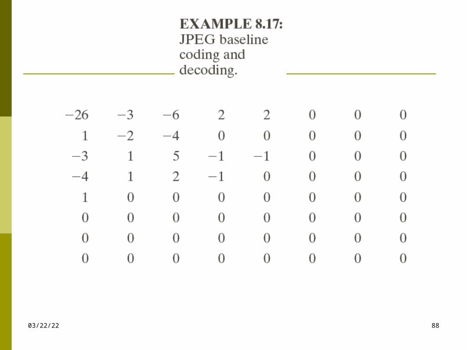
04/19/23 85

04/19/23 86

04/19/23 87

04/19/23 88

04/19/23 89

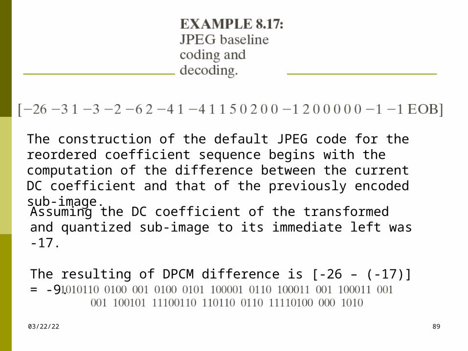
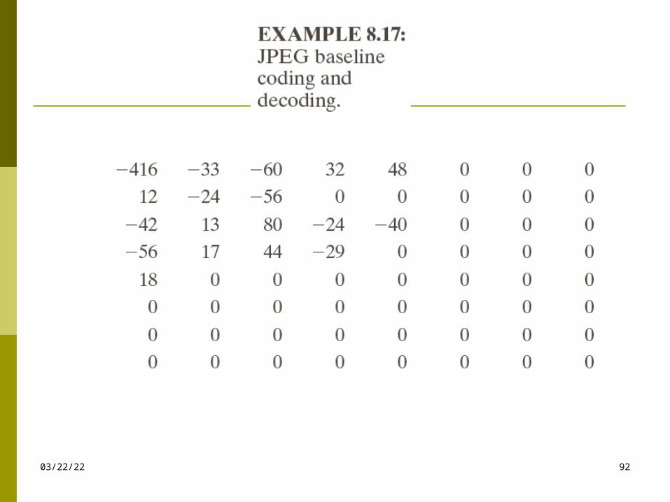
The construction of the default JPEG code for the reordered coefficient sequence begins with the computation of the difference between the current DC coefficient and that of the previously encoded sub-image.

Assuming the DC coefficient of the transformed and quantized sub-image to its immediate left was -17.

The resulting of DPCM difference is [-26 – (-17)] = -9.

04/19/23 90

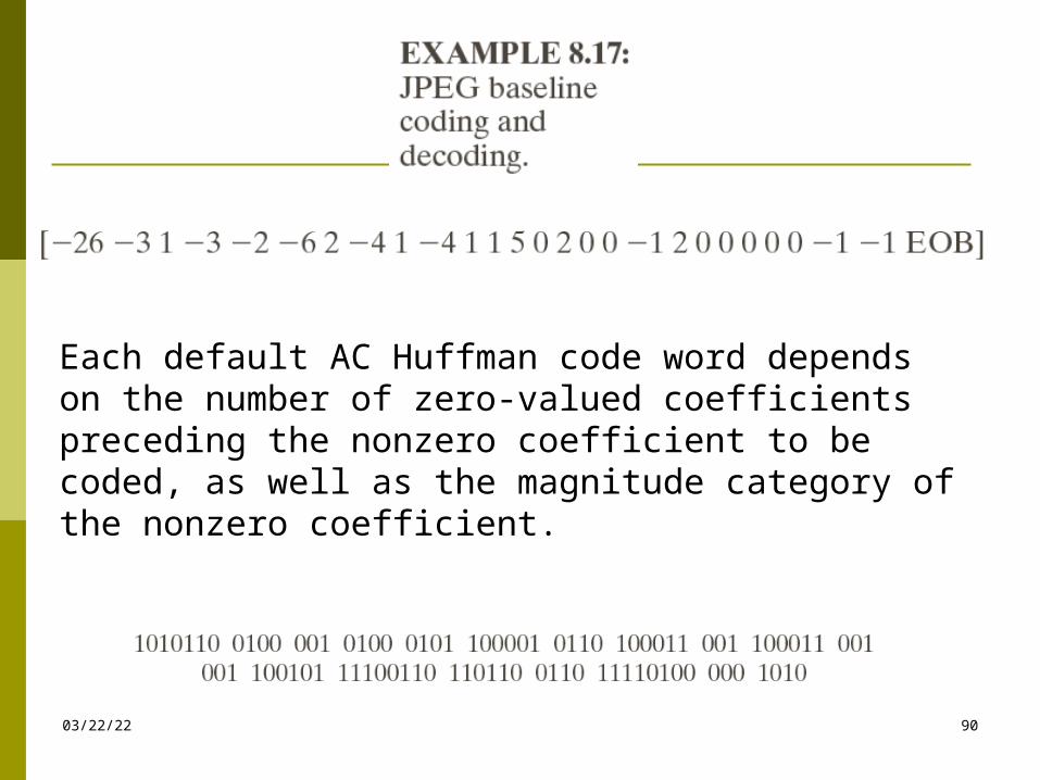
Each default AC Huffman code word depends on the number of zero-valued coefficients preceding the nonzero coefficient to be coded, as well as the magnitude category of the nonzero coefficient.

04/19/23 91

04/19/23 92

04/19/23 93

04/19/23 94

04/19/23 95

04/19/23 96

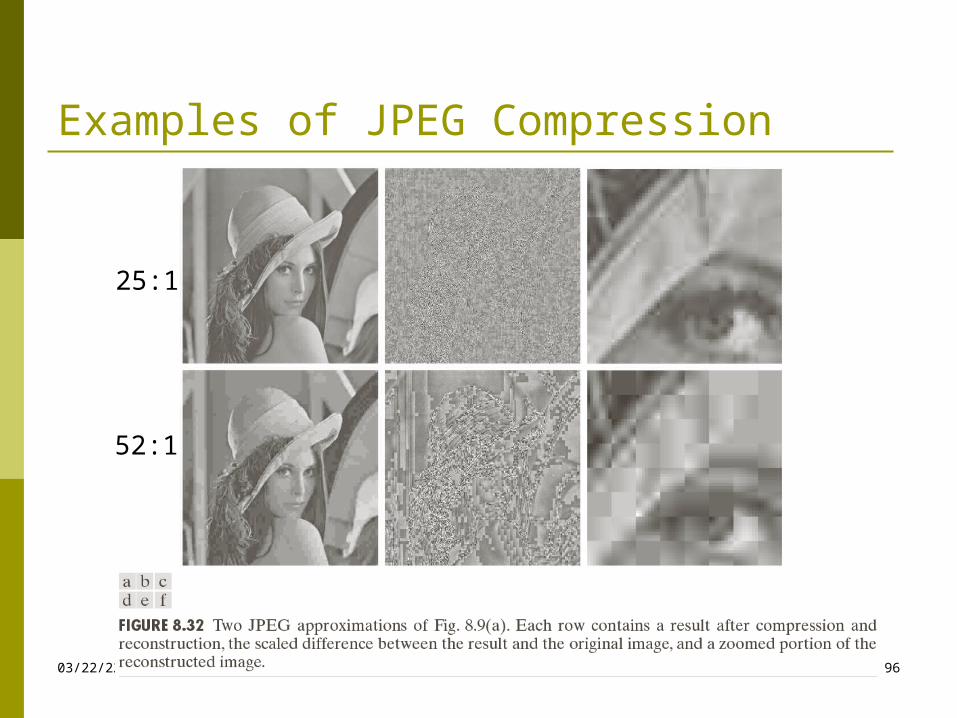
Examples of JPEG Compression

25:1

52:1

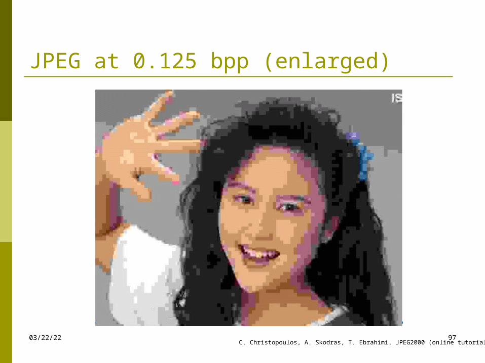
JPEG at 0.125 bpp (enlarged)

04/19/23 97C. Christopoulos, A. Skodras, T. Ebrahimi, JPEG2000 (online tutorial)

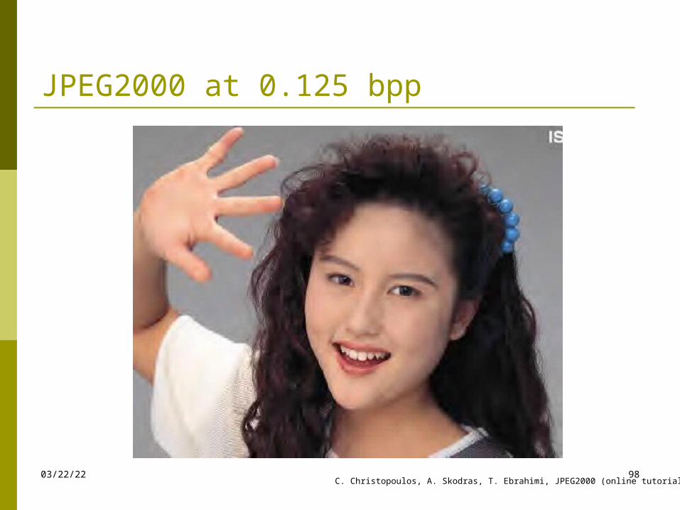
JPEG2000 at 0.125 bpp

04/19/23 98C. Christopoulos, A. Skodras, T. Ebrahimi, JPEG2000 (online tutorial)

Documents

CSE 489-02 & CSE589-02 Multimedia Processing Lecture 7. Image Compression Spring 2009