CSE 460Linear Programming"

Today we will look at"

• Classes of Optimization Problems"

• Linear Programming"

• The Simplex Algorithm"

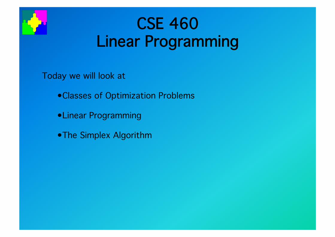
Classes of Optimization Problems"

maxv x

f (v x ) subject to C(v x )

Optimization"

unconstrained" constrained"

linear" non-linear"

quadratic" ..."integer"real-valued"

..."

..."

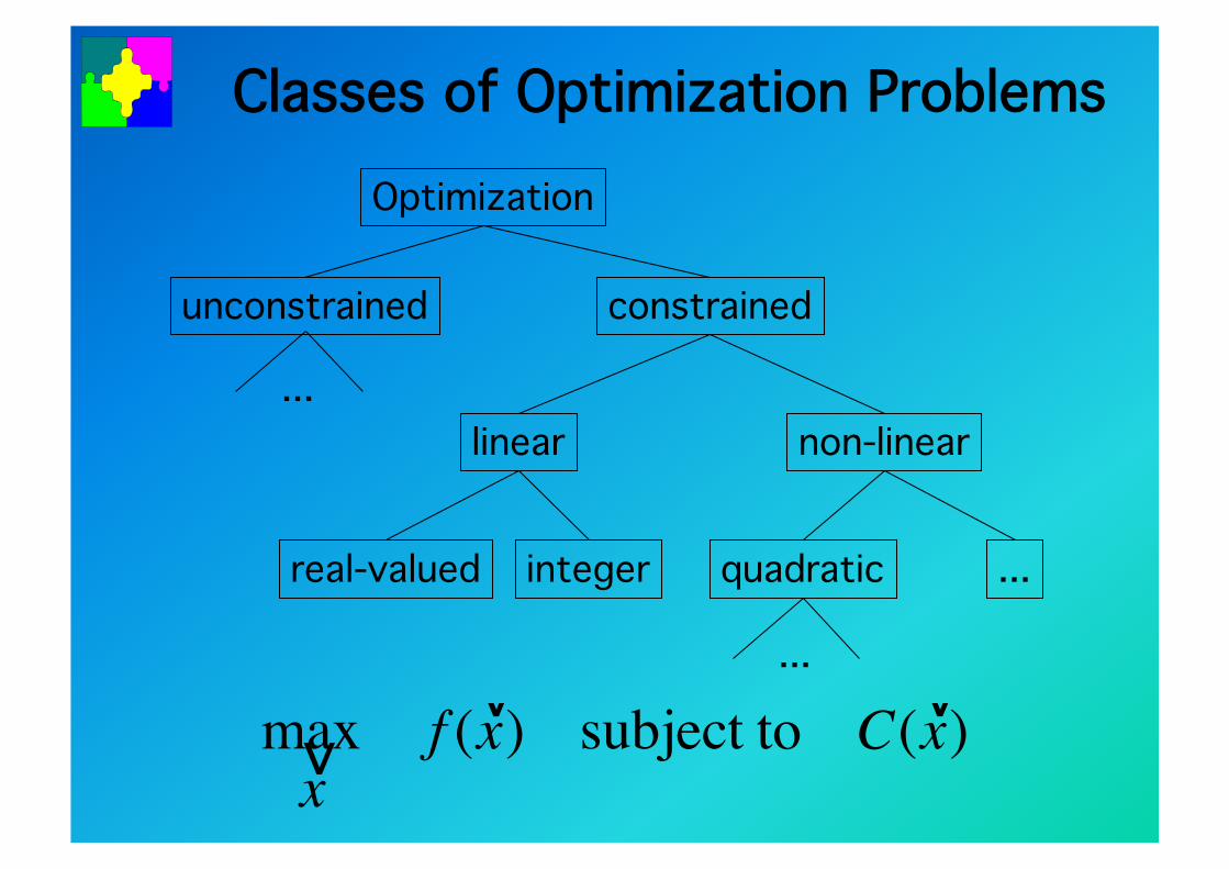
Solution Spaces"A solution space or feasible region is the union of all points"in the domain that satisfy the problem constraints. "The most important distinction is between convex and "non-convex solution spaces:"

Convexity means that any interpolation between "feasible points only yields feasible points."

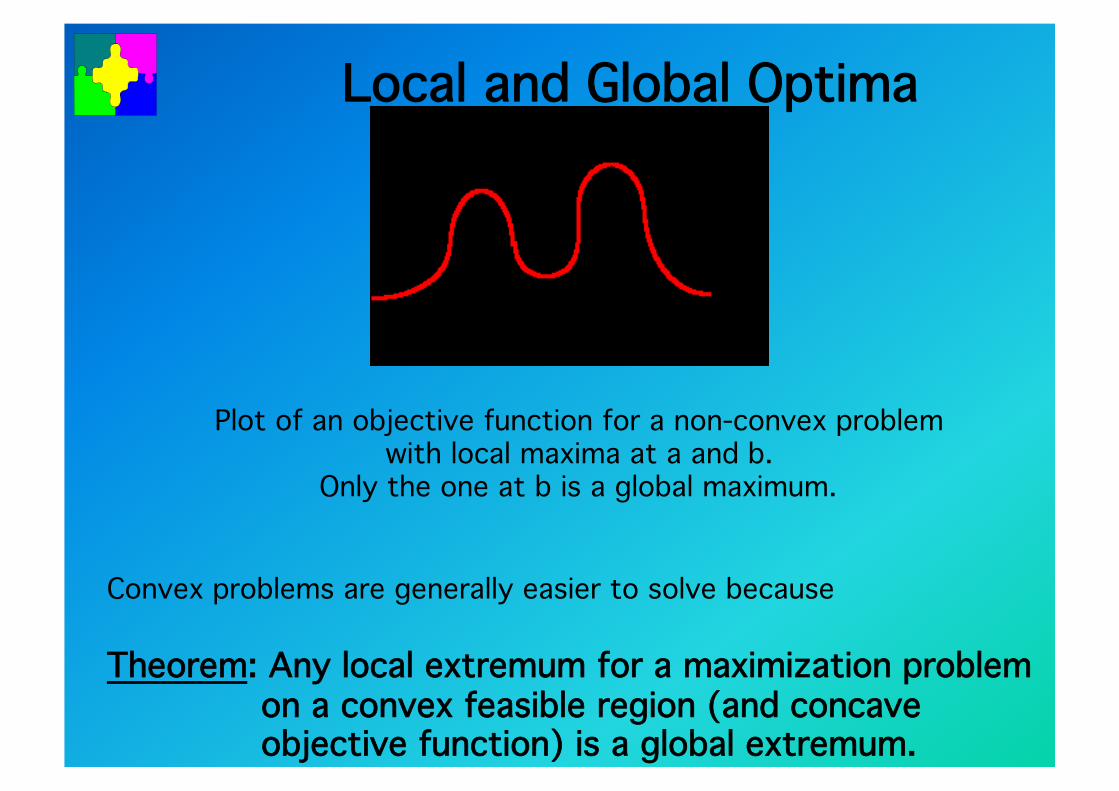
Local and Global Optima"

Convex problems are generally easier to solve because"

Theorem: Any local extremum for a maximization problem"" on a convex feasible region (and concave "" objective function) is a global extremum."

Plot of an objective function for a non-convex problem"with local maxima at a and b. "

Only the one at b is a global maximum. "

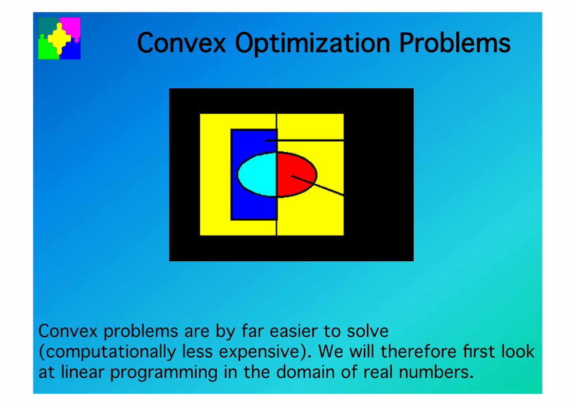
Convex Optimization Problems"

Convex problems are by far easier to solve "(computationally less expensive). We will therefore first look "at linear programming in the domain of real numbers."

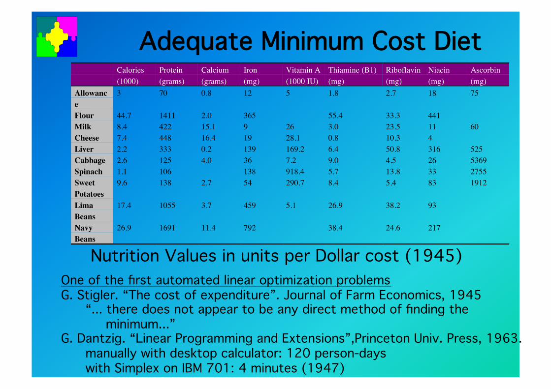
Adequate Minimum Cost Diet"Calories(1000)

Protein(grams)

Calcium(grams)

Iron(mg)

Vitamin A(1000 IU)

Thiamine (B1)(mg)

Riboflavin(mg)

Niacin(mg)

Ascorbin(mg)

Allowance

3 70 0.8 12 5 1.8 2.7 18 75

Flour 44.7 1411 2.0 365 55.4 33.3 441Milk 8.4 422 15.1 9 26 3.0 23.5 11 60Cheese 7.4 448 16.4 19 28.1 0.8 10.3 4Liver 2.2 333 0.2 139 169.2 6.4 50.8 316 525Cabbage 2.6 125 4.0 36 7.2 9.0 4.5 26 5369Spinach 1.1 106 138 918.4 5.7 13.8 33 2755SweetPotatoes

9.6 138 2.7 54 290.7 8.4 5.4 83 1912

LimaBeans

17.4 1055 3.7 459 5.1 26.9 38.2 93

NavyBeans

26.9 1691 11.4 792 38.4 24.6 217

Nutrition Values in units per Dollar cost (1945)"One of the first automated linear optimization problems"G. Stigler. “The cost of expenditure”. Journal of Farm Economics, 1945"

“... there does not appear to be any direct method of finding the " minimum...”"

G. Dantzig. “Linear Programming and Extensions”,Princeton Univ. Press, 1963."manually with desktop calculator: 120 person-days"with Simplex on IBM 701: 4 minutes (1947)"

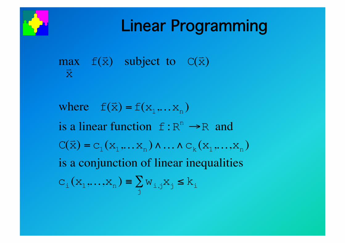
Linear Programming"

€

maxv x

f(v x ) subject to C(v x )

where f(v x ) =f(x1,Kxn )is a linear function f :Rn →R and C(v x ) =c1(x1,Kxn)∧K∧ck (x1,K,xn)is a conjunction of linear inequalitiesci(x1,K,xn ) ≡ wi,jxj ≤ki

j∑

Gauss-Jordan Elimination"

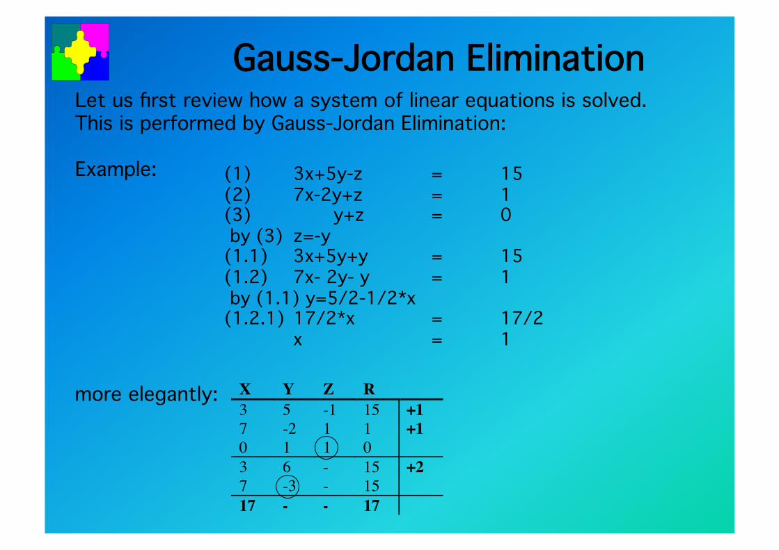
(1) "3x+5y-z "= "15"(2) "7x-2y+z "= "1"(3) " y+z "= "0" by (3) "z=-y"(1.1) "3x+5y+y "= "15"(1.2) "7x- 2y- y "= "1" by (1.1) y=5/2-1/2*x"(1.2.1) "17/2*x" "= "17/2"

"x " "= "1"

Let us first review how a system of linear equations is solved."This is performed by Gauss-Jordan Elimination:"

Example:"

more elegantly:" X Y Z R3 5 -1 15 +17 -2 1 1 +10 1 1 03 6 - 15 +27 -3 - 1517 - - 17

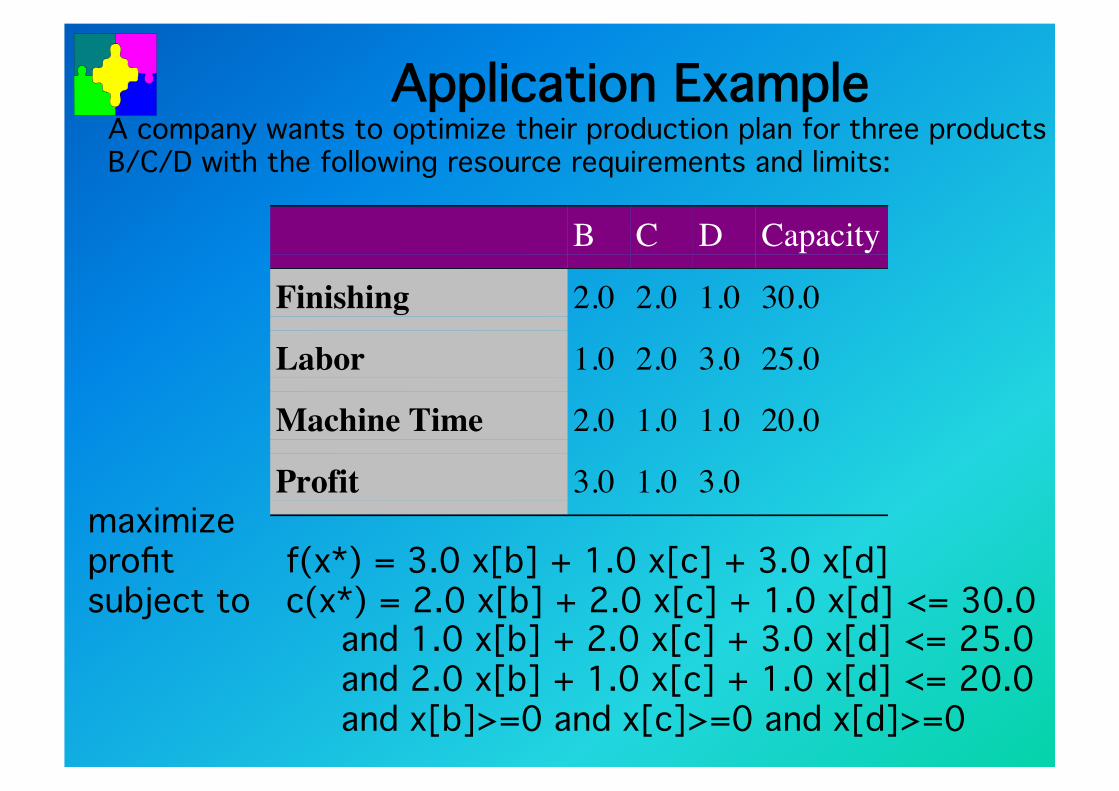
Application Example"

B C D Capacity

Finishing 2.0 2.0 1.0 30.0

Labor 1.0 2.0 3.0 25.0

Machine Time 2.0 1.0 1.0 20.0

Profit 3.0 1.0 3.0maximize"profit "f(x*) = 3.0 x[b] + 1.0 x[c] + 3.0 x[d]"subject to "c(x*) = 2.0 x[b] + 2.0 x[c] + 1.0 x[d] <= 30.0"

" " and 1.0 x[b] + 2.0 x[c] + 3.0 x[d] <= 25.0"" " and 2.0 x[b] + 1.0 x[c] + 1.0 x[d] <= 20.0"" " and x[b]>=0 and x[c]>=0 and x[d]>=0 "

A company wants to optimize their production plan for three products"B/C/D with the following resource requirements and limits:"

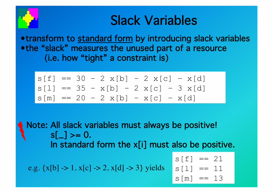
Slack Variables"• transform to standard form by introducing slack variables"• the “slack” measures the unused part of a resource

"(i.e. how “tight” a constraint is)"

Note: All slack variables must always be positive! " s[_] >= 0. "

"In standard form the x[i] must also be positive."

e.g. {x[b] -> 1, x[c] -> 2, x[d] -> 3} yields

s[f] == 30 – 2 x[b] – 2 x[c] – x[d] s[l] == 35 – x[b] – 2 x[c] – 3 x[d] s[m] == 20 – 2 x[b] – x[c] – x[d]

s[f] == 21 s[l] == 11 s[m] == 13

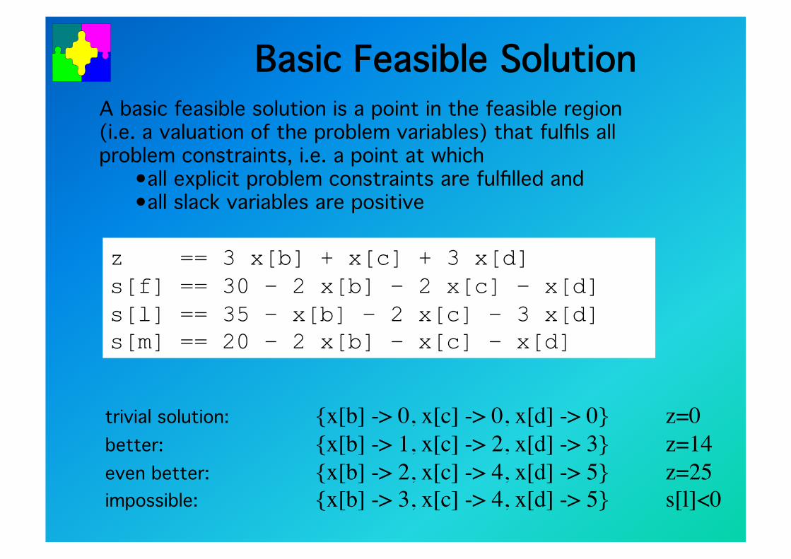
Basic Feasible Solution"A basic feasible solution is a point in the feasible region"(i.e. a valuation of the problem variables) that fulfils all "problem constraints, i.e. a point at which "

• all explicit problem constraints are fulfilled and"• all slack variables are positive"

trivial solution: " "{x[b] -> 0, x[c] -> 0, x[d] -> 0} z=0"better: " " "{x[b] -> 1, x[c] -> 2, x[d] -> 3} z=14"even better: " "{x[b] -> 2, x[c] -> 4, x[d] -> 5} z=25"impossible: " "{x[b] -> 3, x[c] -> 4, x[d] -> 5} s[l]<0

z == 3 x[b] + x[c] + 3 x[d] s[f] == 30 – 2 x[b] – 2 x[c] – x[d] s[l] == 35 – x[b] – 2 x[c] – 3 x[d] s[m] == 20 – 2 x[b] – x[c] – x[d]

Simplex Algorithm: Idea"

The solution to a linear programming problem can be found"by iterative improvement:"

(1) take any feasible solution"(2) check whether any resources are left"(3) check whether exchanging some “activity” (product)" improves the solution"(4) if so, exchange & repeat from step (2)" otherwise the optimum is reached."

Simplex: Geometric Interpretation"

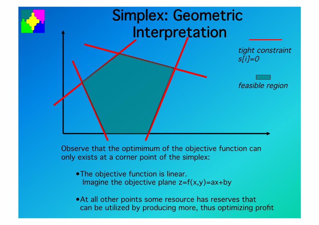
Observe that the optimimum of the objective function can"only exists at a corner point of the simplex:"

• The objective function is linear. " Imagine the objective plane z=f(x,y)=ax+by"

• At all other points some resource has reserves that can be utilized by producing more, thus optimizing profit"

feasible region!

tight constraint!s[i]=0"

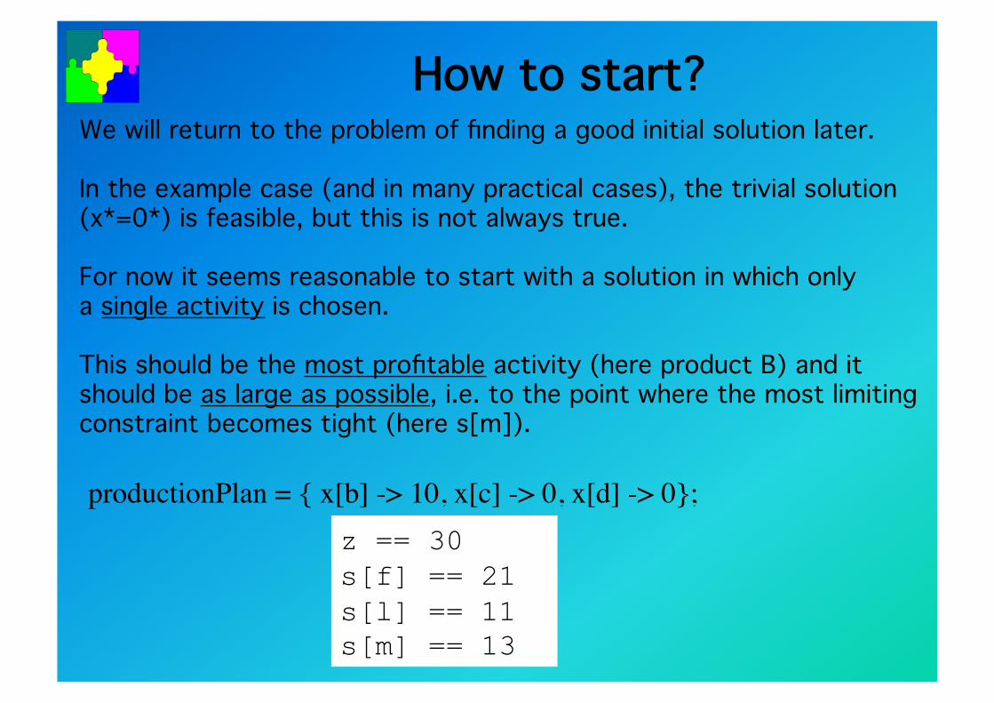
How to start?"We will return to the problem of finding a good initial solution later. "

In the example case (and in many practical cases), the trivial solution "(x*=0*) is feasible, but this is not always true."

For now it seems reasonable to start with a solution in which only "a single activity is chosen. "

This should be the most profitable activity (here product B) and it "should be as large as possible, i.e. to the point where the most limiting "constraint becomes tight (here s[m]). "

productionPlan = { x[b] -> 10, x[c] -> 0, x[d] -> 0}; z == 30 s[f] == 21 s[l] == 11 s[m] == 13

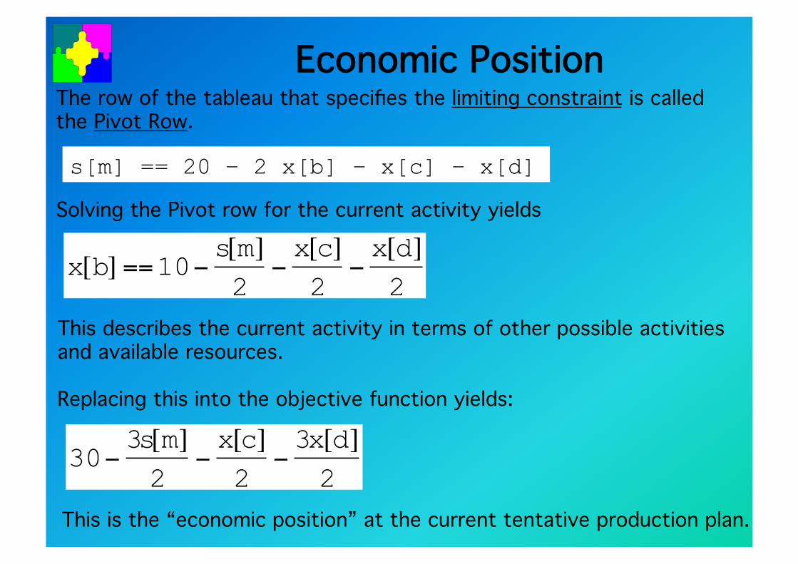
Economic Position"The row of the tableau that specifies the limiting constraint is called"the Pivot Row."

Solving the Pivot row for the current activity yields"

This is the “economic position” at the current tentative production plan."

This describes the current activity in terms of other possible activities"and available resources."

Replacing this into the objective function yields:"

s[m] == 20 – 2 x[b] – x[c] – x[d]

€

x[b] ==10−s[m]2

−x[c]2

−x[d]2

€

30−3s[m]2

−x[c]2

−3x[d]2

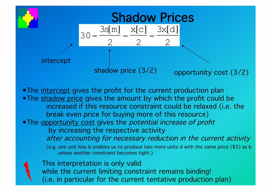
Shadow Prices"

intercept"shadow price (3/2)" opportunity cost (3/2)"

This interpretation is only valid"while the current limiting constraint remains binding!"(i.e. in particular for the current tentative production plan)"

• The intercept gives the profit for the current production plan"• The shadow price gives the amount by which the profit could be

"increased if this resource constraint could be relaxed (i.e. the "break even price for buying more of this resource)"

• The opportunity cost gives the potential increase of profit " by increasing the respective activity "after accounting for necessary reduction in the current activity!(e.g. one unit less b enables us to produce two more units d with the same price ($3) as b

unless another constraint becomes tight.)"

€

30−3s[m]2

−x[c]2

−3x[d]2

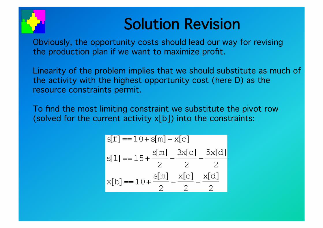
Solution Revision"Obviously, the opportunity costs should lead our way for revising"the production plan if we want to maximize profit."

Linearity of the problem implies that we should substitute as much of"the activity with the highest opportunity cost (here D) as the "resource constraints permit."

To find the most limiting constraint we substitute the pivot row "(solved for the current activity x[b]) into the constraints:"

€

s[f] ==10+s[m] −x[c]

s[l] ==15+s[m]2

−3x[c]2

−5x[d]2

x[b] ==10+s[m]2

−x[c]2

−x[d]2

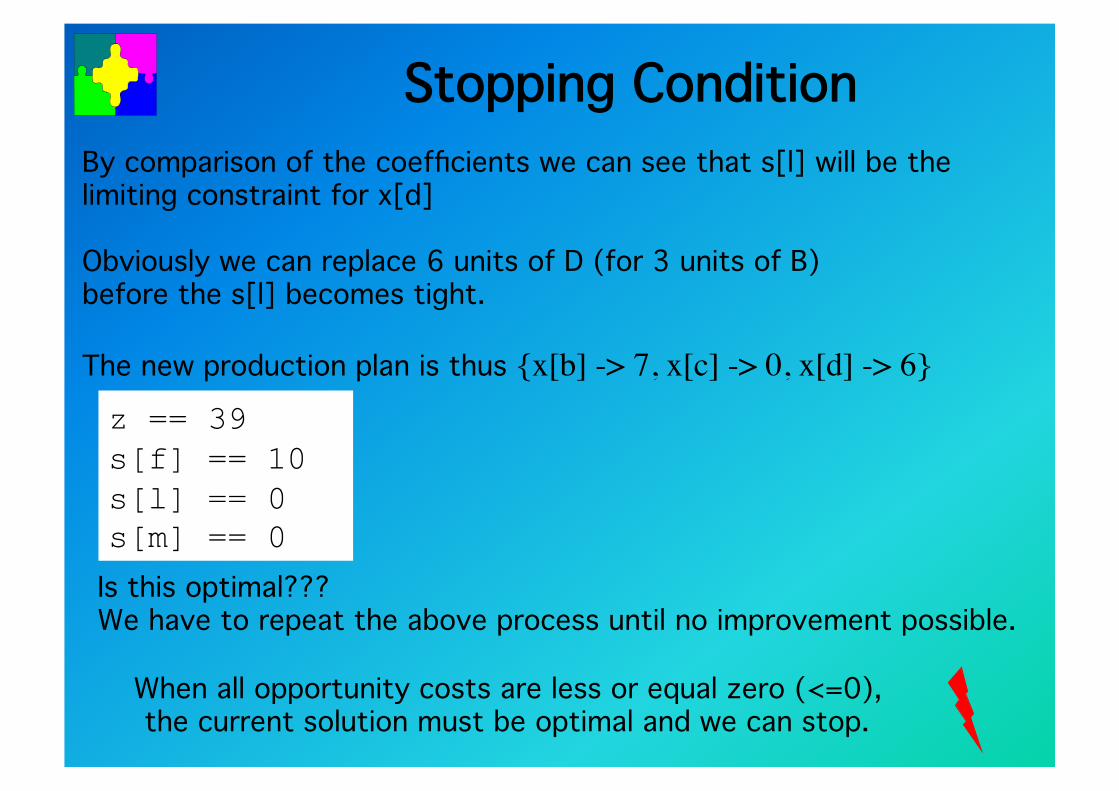
Stopping Condition"By comparison of the coefficients we can see that s[l] will be the "limiting constraint for x[d] "

Obviously we can replace 6 units of D (for 3 units of B)"before the s[l] becomes tight."

The new production plan is thus {x[b] -> 7, x[c] -> 0, x[d] -> 6}

Is this optimal???"We have to repeat the above process until no improvement possible."

What is a reasonable stopping condition?"When all opportunity costs are less or equal zero (<=0),"the current solution must be optimal and we can stop."

z == 39 s[f] == 10 s[l] == 0 s[m] == 0

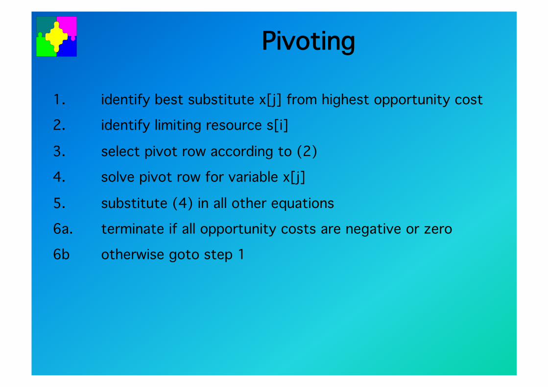
Pivoting"1. "identify best substitute x[j] from highest opportunity cost"

2. "identify limiting resource s[i]"

3. "select pivot row according to (2)"

4. "solve pivot row for variable x[j]"

5. "substitute (4) in all other equations"

6a. "terminate if all opportunity costs are negative or zero"

6b "otherwise goto step 1"

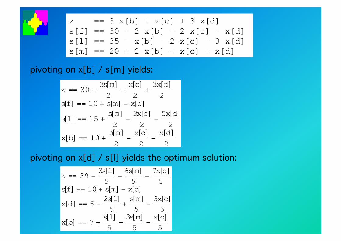
pivoting on x[b] / s[m] yields:"

pivoting on x[d] / s[l] yields the optimum solution:"

€

z == 3 x[b] + x[c] + 3 x[d] s[f] == 30 – 2 x[b] – 2 x[c] – x[d] s[l] == 35 – x[b] – 2 x[c] – 3 x[d] s[m] == 20 – 2 x[b] – x[c] – x[d]

€

z == 30 −3s[m]2

−x[c]2

+3x[d]2

s[f] == 10 + s[m] − x[c]

s[l] == 15 +s[m]2

−3x[c]2

−5x[d]2

x[b] == 10 +s[m]2

−x[c]2

−x[d]2

€

z == 39 −3s[l]5

−6s[m]5

−7x[c]5

s[f] == 10 + s[m] − x[c]

x[d] == 6 −2s[l]5

+s[m]5

−3x[c]5

x[b] == 7 +s[l]5

−3s[m]5

−x[c]5

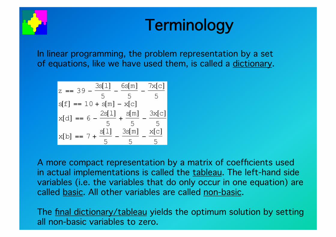
Terminology"In linear programming, the problem representation by a set"of equations, like we have used them, is called a dictionary."

A more compact representation by a matrix of coefficients used"in actual implementations is called the tableau. The left-hand side"variables (i.e. the variables that do only occur in one equation) are "called basic. All other variables are called non-basic."

The final dictionary/tableau yields the optimum solution by setting "all non-basic variables to zero."

€

z == 39 −3s[l]5

−6s[m]5

−7x[c]5

s[f] == 10 + s[m] − x[c]

x[d] == 6 −2s[l]5

+s[m]5

−3x[c]5

x[b] == 7 +s[l]5

−3s[m]5

−x[c]5

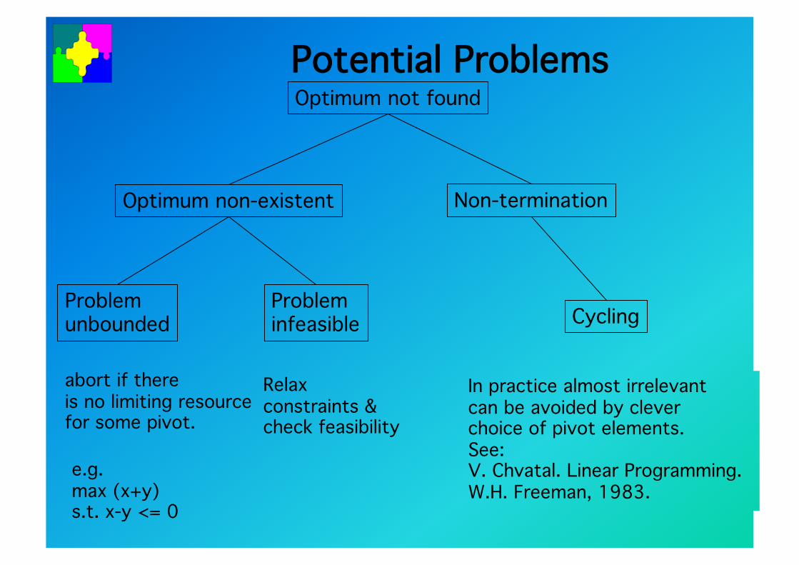
Potential Problems"

Optimum non-existent" Non-termination"

Problem"unbounded"

Problem"infeasible" Cycling"

Optimum not found"

?" ?" ?"In practice almost irrelevant"can be avoided by clever"choice of pivot elements."See: "V. Chvatal. Linear Programming."W.H. Freeman, 1983."

Relax "constraints &"check feasibility"

abort if there"is no limiting resource"for some pivot."

e.g."max (x+y)"s.t. x-y <= 0"

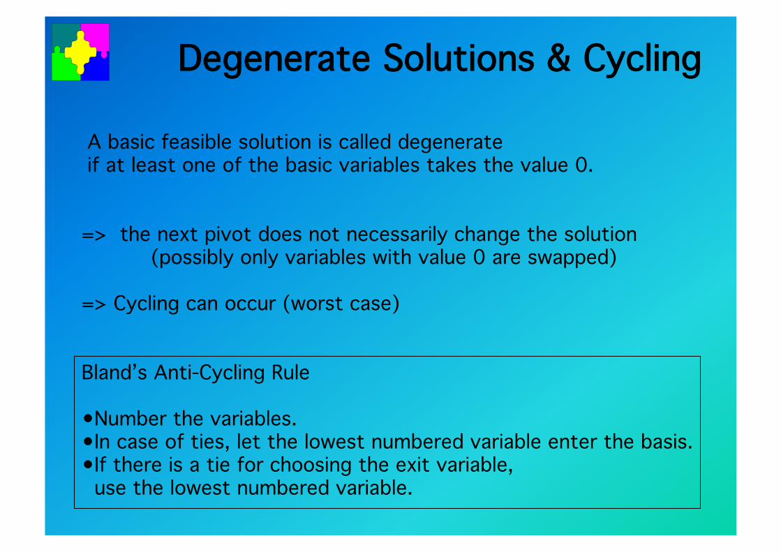
Degenerate Solutions & Cycling"A basic feasible solution is called degenerate"if at least one of the basic variables takes the value 0."

=> the next pivot does not necessarily change the solution""(possibly only variables with value 0 are swapped)"

=> Cycling can occur (worst case)"

Bland’s Anti-Cycling Rule"

• Number the variables."• In case of ties, let the lowest numbered variable enter the basis."• If there is a tie for choosing the exit variable, use the lowest numbered variable."

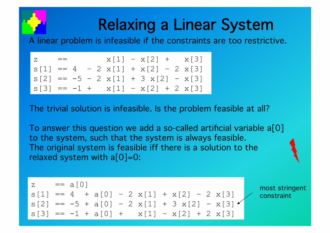
Relaxing a Linear System"A linear problem is infeasible if the constraints are too restrictive."

The trivial solution is infeasible. Is the problem feasible at all?"

To answer this question we add a so-called artificial variable a[0]"to the system, such that the system is always feasible."The original system is feasible iff there is a solution to the"relaxed system with a[0]=0:"

most stringent"constraint"

z == x[1] – x[2] + x[3] s[1] == 4 – 2 x[1] + x[2] – 2 x[3] s[2] == -5 – 2 x[1] + 3 x[2] – x[3] s[3] == -1 + x[1] – x[2] + 2 x[3]

z == a[0] s[1] == 4 + a[0] – 2 x[1] + x[2] – 2 x[3] s[2] == -5 + a[0] – 2 x[1] + 3 x[2] – x[3] s[3] == -1 + a[0] + x[1] – x[2] + 2 x[3]

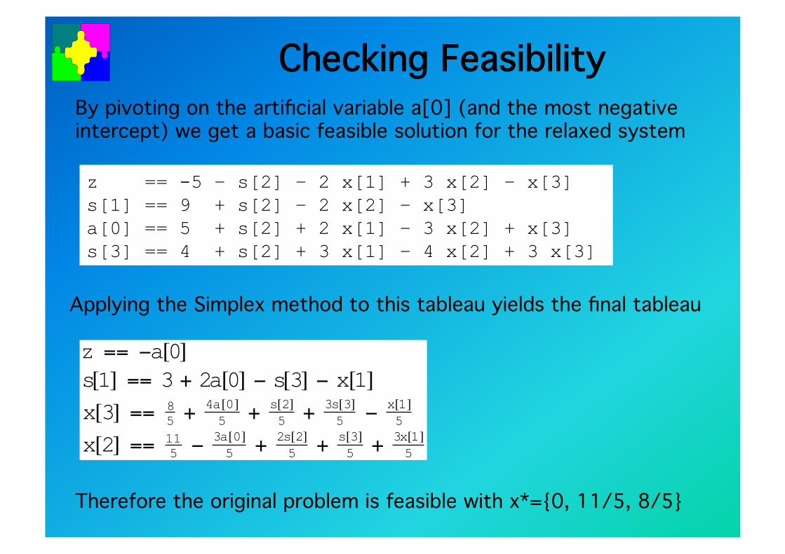
Checking Feasibility"By pivoting on the artificial variable a[0] (and the most negative"intercept) we get a basic feasible solution for the relaxed system"

Applying the Simplex method to this tableau yields the final tableau"

Therefore the original problem is feasible with x*={0, 11/5, 8/5} "

z == -5 – s[2] – 2 x[1] + 3 x[2] – x[3] s[1] == 9 + s[2] – 2 x[2] – x[3] a[0] == 5 + s[2] + 2 x[1] – 3 x[2] + x[3] s[3] == 4 + s[2] + 3 x[1] – 4 x[2] + 3 x[3]

€

z == −a[0]s[1] == 3 + 2a[0] − s[3] − x[1]x[3] == 8

5 + 4a[0]5 + s[2]

5 + 3s[3]5 − x[1]

5

x[2] == 115 − 3a[0]

5 + 2s[2]5 + s[3]

5 + 3x[1]5

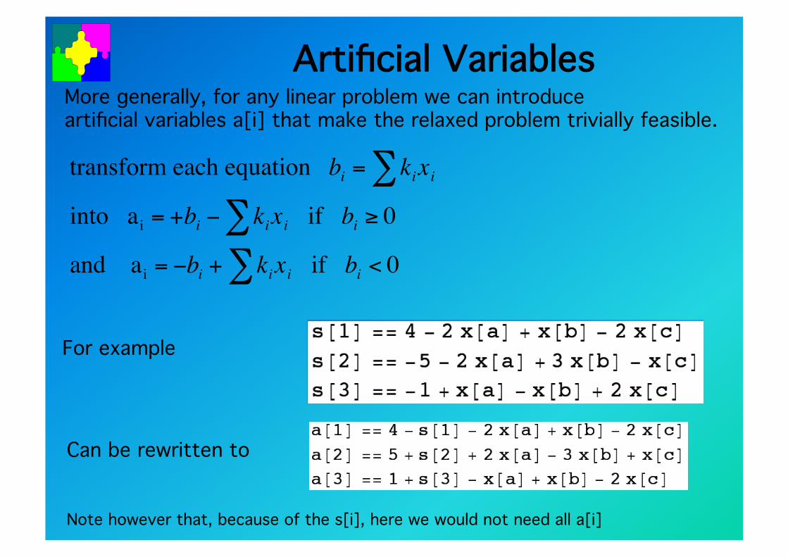
Artificial Variables"More generally, for any linear problem we can introduce "artificial variables a[i] that make the relaxed problem trivially feasible."

€

transform each equation bi = kixi∑into ai = +bi − kixi if bi ≥ 0∑and ai = −bi + kixi if bi < 0∑

For example"

Note however that, because of the s[i], here we would not need all a[i]"

Can be rewritten to"

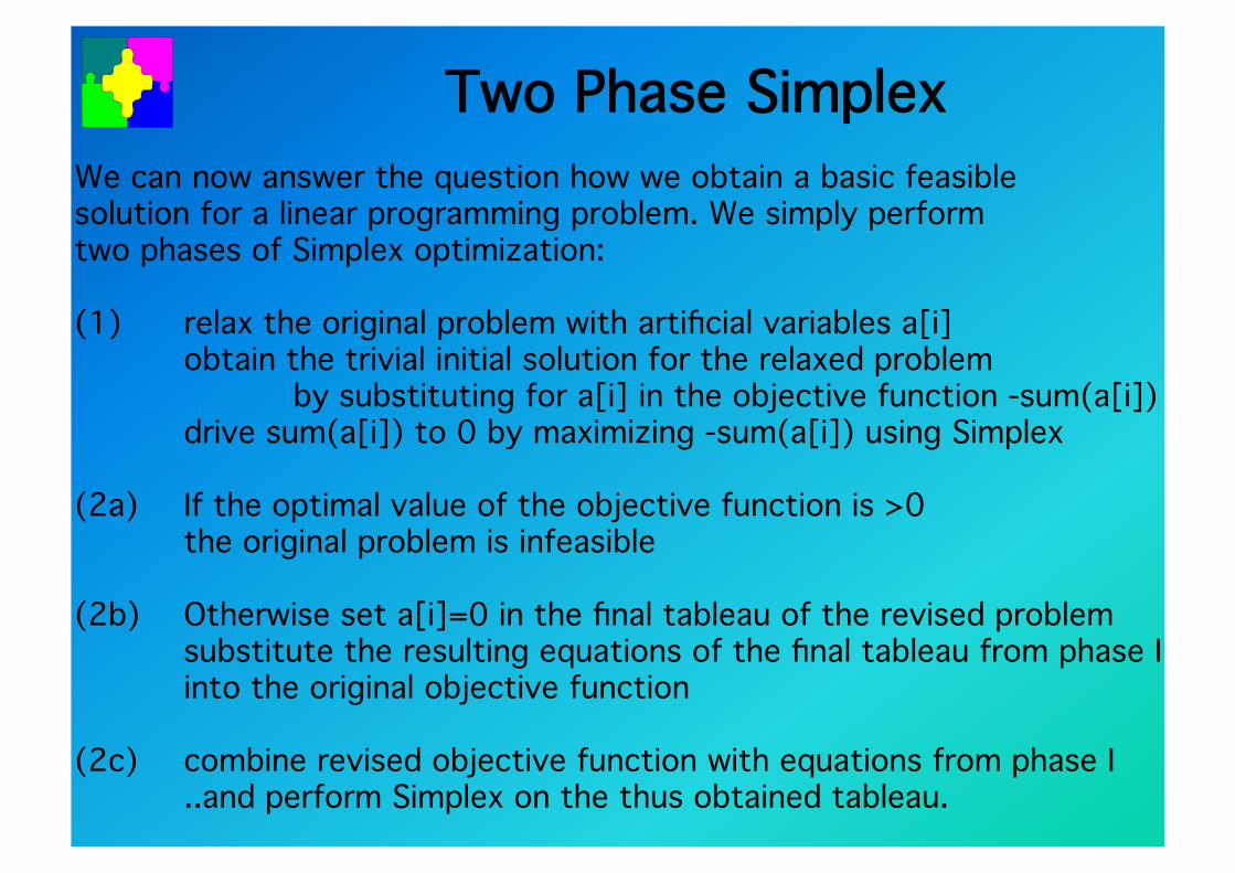
Two Phase Simplex"We can now answer the question how we obtain a basic feasible "solution for a linear programming problem. We simply perform "two phases of Simplex optimization:"

(1) "relax the original problem with artificial variables a[i]""obtain the trivial initial solution for the relaxed problem "" "by substituting for a[i] in the objective function -sum(a[i])""drive sum(a[i]) to 0 by maximizing -sum(a[i]) using Simplex"

(2a) "If the optimal value of the objective function is >0""the original problem is infeasible"

(2b) "Otherwise set a[i]=0 in the final tableau of the revised problem""substitute the resulting equations of the final tableau from phase I""into the original objective function"

(2c) "combine revised objective function with equations from phase I""..and perform Simplex on the thus obtained tableau."

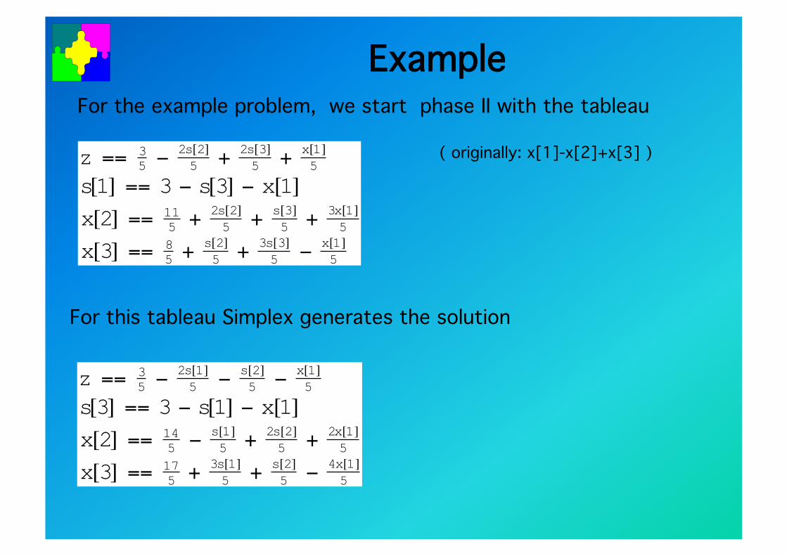
Example "For the example problem, we start phase II with the tableau"

For this tableau Simplex generates the solution"

( originally: x[1]-x[2]+x[3] )"

€

z == 35 −

2s[2]5 + 2s[3]

5 + x[1]5

s[1] == 3 − s[3] − x[1]x[2] == 11

5 + 2s[2]5 + s[3]

5 + 3x[1]5

x[3] == 85 + s[2]

5 + 3s[3]5 − x[1]

5

€

z == 35 −

2s[1]5 − s[2]

5 − x[1]5

s[3] == 3 − s[1] − x[1]x[2] == 14

5 − s[1]5 + 2s[2]

5 + 2x[1]5

x[3] == 175 + 3s[1]

5 + s[2]5 − 4x[1]

5

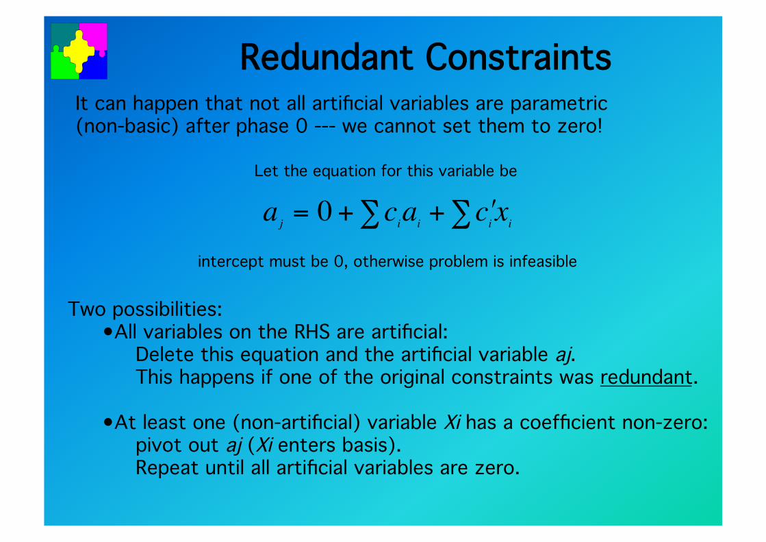
Redundant Constraints "It can happen that not all artificial variables are parametric"(non-basic) after phase 0 --- we cannot set them to zero!"

Two possibilities:"• All variables on the RHS are artificial:"

Delete this equation and the artificial variable aj."This happens if one of the original constraints was redundant.

• At least one (non-artificial) variable Xi has a coefficient non-zero:"pivot out aj (Xi enters basis)."Repeat until all artificial variables are zero."

Let the equation for this variable be"

aj = 0 + ciai∑ + ʹ′ c i xi∑

intercept must be 0, otherwise problem is infeasible"

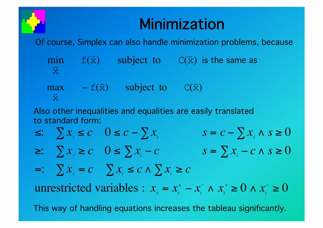
Minimization"Of course, Simplex can also handle minimization problems, because"

Also other inequalities and equalities are easily translated"to standard form:"

€

minv x

f(v x ) subject to C(v x ) is the same as"

€

maxv x

− f(v x ) subject to C(v x )

≤: xi ≤ c∑ 0 ≤ c − xi∑ s = c − xi ∧ s ≥ 0∑

≥: x∑ i ≥ c 0 ≤ xi − c∑ s = xi − c∧ s ≥ 0∑

=: xi = c∑ xi ≤ c∑ ∧ xi ≥ c∑

unrestricted variables : xi = xi+ − xi− ∧ xi+ ≥ 0 ∧ xi− ≥ 0This way of handling equations increases the tableau significantly. "

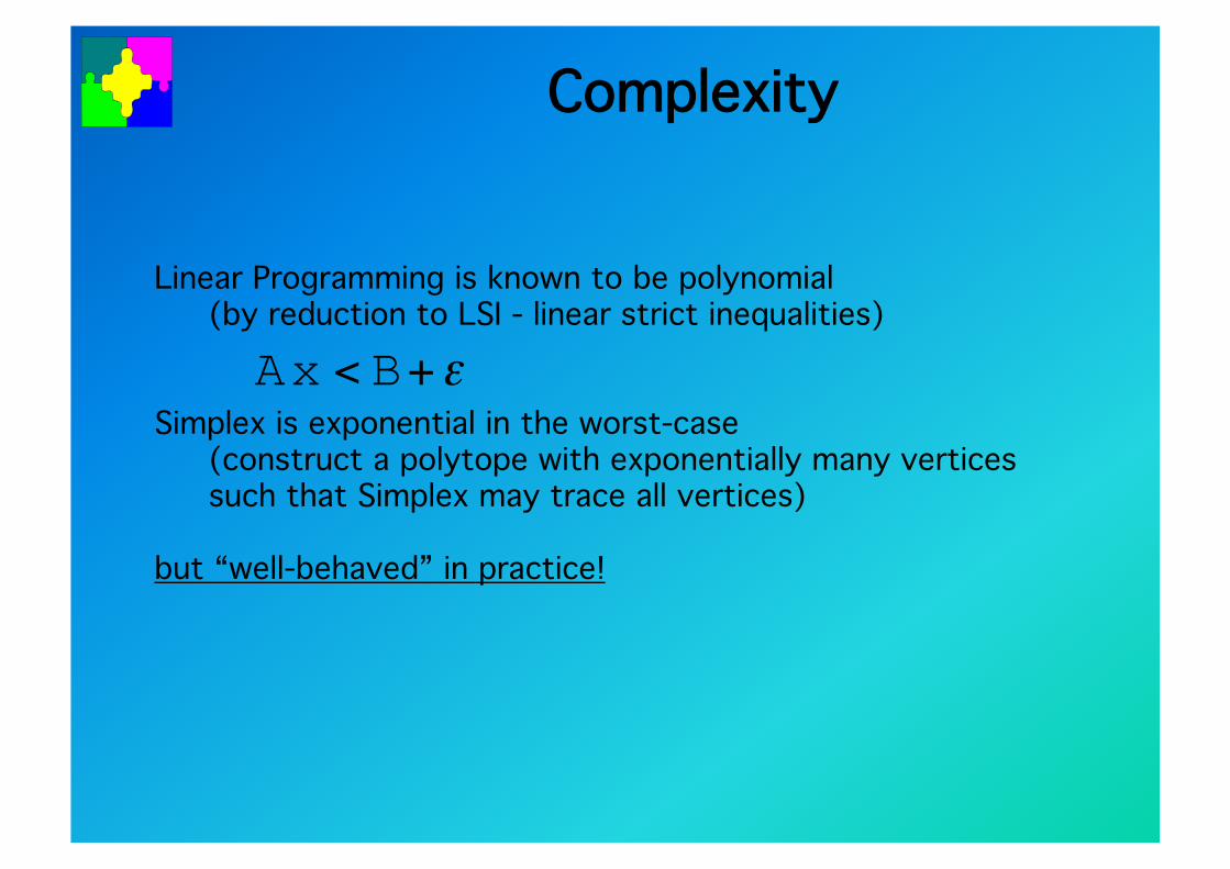
Complexity"

Linear Programming is known to be polynomial"(by reduction to LSI - linear strict inequalities)"

Simplex is exponential in the worst-case"(construct a polytope with exponentially many vertices"such that Simplex may trace all vertices)"

but “well-behaved” in practice!"

€

Ax < B+ε

Summary"Today we have looked at"

• Classes of Optimization Problems"

• Linear Programming"

• The Simplex Algorithm"

Homework"

• Execute Simplex manually on a small problem"

• Read Simplex in Winston and/or Marriott & Stuckey"