Embed Size (px)
Citation preview
CSC 126 2017/2018 1 [email protected]
CSC 126 PHYSICS FOR COMPUTING SYSTEMS
Course Instructor: Dr. Justus Simiyu
Department of Physics, UoN
Course Objective
This is a Physics course for beginners in Bachelor of Science in Computer Science course for the
University of Nairobi. The main objective of the course is to introduce the learner to the basic
principles of Physics applied in computing, specifically electricity, magnetism and semiconductor
Physics. The course is divided into two main parts one being Basic Physics and the second
Semiconductor Physics. In the first section, the learner is introduced to the relationship of Physics
with Computer Science touching on the Physics principles behind the operation of computers at
both hardware and software domain. In the second section, the learner is introduced to
Semiconductor Physics as the building block to basic computing platform of operation such as the
ALU, communication as well as interfacing among others. Upon successful completion of this
course, the learner is expected to be equipped with the knowledge about the physics of these
devices, how they work and how they are integrated in the whole system. This will also equip the
learner with knowledge and ability to implement routines, carry out maintenance and more
importantly have proper judgment on the action to be taken in case of failure or malfunction of
the systems.
Specific Objectives
The specific objectives are as per the topics covered in the entire syllabus.
Introduction
This section introduces the learner to the conception of the devices to be studied later in the
course. The learner is expected to understand the accepted model describing the atomic structure
and atomic interaction that brings about bonding to form a whole system of semiconductor
materials.
Semiconductor p-n junction devices (diodes)
This section introduces the learner to the band model that is used to describe conductivity and
classify materials in terms of conductivity. The section narrows down to semiconductors where
the learner is expected to distinguish between metals, semiconductors and insulators. Since
almost all the active devices used in computers are based on the basic diode characteristics, this
section deals in detail with these characteristics and the various applications according to the
characteristics.
Transistors
After having studied p-n junctions in the previous section, this chapter goes a step further where
several diodes are put together to form transistor devices. In this section, the learner is expected to
know the type of transistors (Bipolar and Field effect transistors), their characteristics and the
configuration models (i.e. common base, common emitter and common collector for the case of
bipolar junction transistors). The learner is also expected to gain knowledge on where and for
what requirements the transistor modes are used. Various biasing circuits are also dealt with in
detail in this section. This addresses the issue of determining practically bias points of the
transistors and can be ascertained as labelled by transistor manufactures and how they are
integrated in the systems.
CSC 126 2017/2018 2 [email protected]
Logic circuit applications
This section utilizes the knowledge acquired on transistors to apply in computer logic operations.
Since logic is the backbone of system operations of computers’ integrated circuitry, it is
important that the learner gets informed about the various logic items that are used. The logic
items dealt with in this section are AND, OR, NAND, NOR, INVERTER, EXCLUSIVE OR and
INHIBIT (ENABLE) operations and highlights the areas they are applied in the integrated
circuitry.
COURSE OUTLINE
PART ONE: BASIC PHYSICS
1. Electricity
Electrostatics: charge force, electrics fields, Coulomb’s law, Gauss’s law, electrics
potential, electric energy, capacitance
2. DC circuits
Current, Ohms law, resistance, DC circuits, Kirchhoff’s laws, voltage sources, circuit
analysis
3. Magnetism
Magnetics properties of matter, magnetic fileds, Biot-savart law, force law, applications
4. Electromagnetism
Faradays law, Lenz’s law, induced emf, inductance, applications
5. Waves
Wave equation, elastic waves in solids, progressive waves, interference, and reflection of
waves.
6. Optics
Reflection and refraction at planar and a planar surfaces, fibre optics, optical instruments.
PART TWO: SEMICONDUCTOR ELECTRONICS
A. INTRODUCTION
The atomic structure, Atomic and molecular bonds. Ionic bonding. Covalent bonding.
Metallic bonds. Insulators and semiconductors.
B. PHYSICS OF SEMICONDUCTOR MATERIALS
Band model.
Intrinsic semiconductors. Conduction by electrons and holes. Carrier concentration.
Extrinsic semiconductors.
Photoconduction and photovoltaic effects.
The p-n junction. I-V characteristics.
Diodes: resistance; Zener, tunnel, photo and light emitting diodes. Diode circuits.
Transistors: bipolar junction transistor. Common base, common emitter and common
collector: configuration and their characteristics. Transistor circuits. The transistor as a
switch. Logic circuit applications. Field effect transistor.
Pre-requisites: High School Physics
Delivery
Lectures, tutorials, supervised laboratories.
CSC 126 2017/2018 3 [email protected]
Reference books
1. Physics for Scientist and Engineers, by Serway
2. University Physics by Pierce
3. Principles of Physics by Ohanian
4. Physics by Halliday and Resnick
5. Advanced Level Physics by Nelkon and Parker
6. Elementary semiconductor Physics by Writ, HC. Cho. QC 11 .w93
7. Handbook of semiconductor electronics by Hunter, L.P 3rd Ed. TK 7872 .S4H8 1970
8. Introduction to physics of semiconductor devices by Roulston D. Cho Qc 611 .R86
9. Physics of semiconductor devices by SM Sze. TK 7871 85 .S988 1981
10. Integrated electronics by Millman and Halkias
© First prepared 2004, reprinted 2005, 2006, 2010, revised 2011, 2012, 2016, 2017, 2018
CSC 126 2017/2018 4 [email protected]
PART ONE: BASIC PHYSICS
I Electrostatics
1 Properties of Electric Charges
Simple experiments used to demonstrate the existence of electric forces and charges are for
example:
Running a comb through hair on dry day, the comb starts to attract bits of papers.
Inflated balloon is rubbed with wool. The balloon adheres to the wall or the ceiling of a
room
When materials behave like this, they are said to be electrified or to have become electrically
charged
During wet day, excessive amount of moisture can lead to a leakage of charge from the
electrified body to the earth by various conducting path
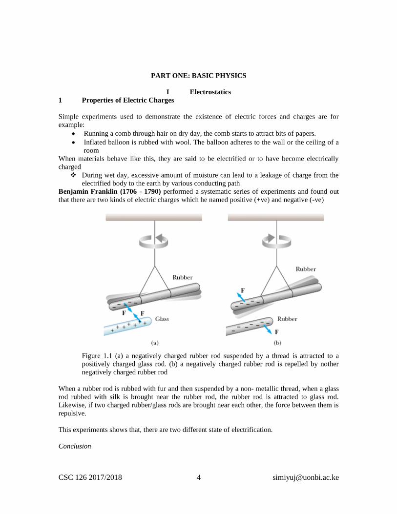
Benjamin Franklin (1706 - 1790) performed a systematic series of experiments and found out
that there are two kinds of electric charges which he named positive (+ve) and negative (-ve)
Figure 1.1 (a) a negatively charged rubber rod suspended by a thread is attracted to a
positively charged glass rod. (b) a negatively charged rubber rod is repelled by nother
negatively charged rubber rod
When a rubber rod is rubbed with fur and then suspended by a non- metallic thread, when a glass
rod rubbed with silk is brought near the rubber rod, the rubber rod is attracted to glass rod.
Likewise, if two charged rubber/glass rods are brought near each other, the force between them is
repulsive.
This experiments shows that, there are two different state of electrification.
Conclusion
CSC 126 2017/2018 5 [email protected]
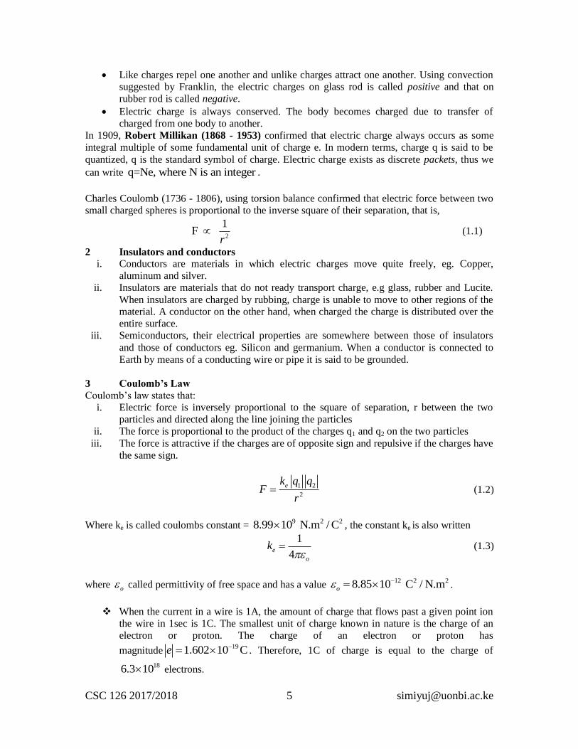
Like charges repel one another and unlike charges attract one another. Using convection
suggested by Franklin, the electric charges on glass rod is called positive and that on
rubber rod is called negative.
Electric charge is always conserved. The body becomes charged due to transfer of
charged from one body to another.
In 1909, Robert Millikan (1868 - 1953) confirmed that electric charge always occurs as some
integral multiple of some fundamental unit of charge e. In modern terms, charge q is said to be
quantized, q is the standard symbol of charge. Electric charge exists as discrete packets, thus we
can write q=Ne, where N is an integer .
Charles Coulomb (1736 - 1806), using torsion balance confirmed that electric force between two
small charged spheres is proportional to the inverse square of their separation, that is,
2
1F
r (1.1)
2 Insulators and conductors
i. Conductors are materials in which electric charges move quite freely, eg. Copper,
aluminum and silver.
ii. Insulators are materials that do not ready transport charge, e.g glass, rubber and Lucite.
When insulators are charged by rubbing, charge is unable to move to other regions of the
material. A conductor on the other hand, when charged the charge is distributed over the
entire surface.
iii. Semiconductors, their electrical properties are somewhere between those of insulators
and those of conductors eg. Silicon and germanium. When a conductor is connected to
Earth by means of a conducting wire or pipe it is said to be grounded.
3 Coulomb’s Law
Coulomb’s law states that:
i. Electric force is inversely proportional to the square of separation, r between the two
particles and directed along the line joining the particles
ii. The force is proportional to the product of the charges q1 and q2 on the two particles
iii. The force is attractive if the charges are of opposite sign and repulsive if the charges have
the same sign.
1 2
2
ek q qF
r (1.2)
Where ke is called coulombs constant = 9 2 28.99 10 N.m / C , the constant ke is also written
1
4e
o
k
(1.3)
where o called permittivity of free space and has a value 12 2 28.85 10 C / N.mo .
When the current in a wire is 1A, the amount of charge that flows past a given point ion
the wire in 1sec is 1C. The smallest unit of charge known in nature is the charge of an
electron or proton. The charge of an electron or proton has
magnitude191.602 10 Ce . Therefore, 1C of charge is equal to the charge of
186.3 10 electrons.
CSC 126 2017/2018 6 [email protected]
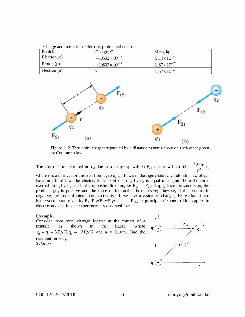
Charge and mass of the electron, proton and neutron
Particle Charge, C Mass, kg
Electron (e) 191.602 10 319.11 10
Proton (p) 191.602 10 271.67 10
Neutron (n) 0 271.67 10
Figure 1. 2. Two point charges separated by a distance r exert a force on each other given
by Coulomb's law.
The electric force exerted on q2 due to a charge q1 written F21 can be written 1 221 2
ek q qF
r r,
where r is a unit vector directed from q1 to q2 as shown in the figure above. Coulomb’s law obeys
Newton’s third law; the electric force exerted on q1 by q2 is equal in magnitude to the force
exerted on q2 by q1 and in the opposite direction, i.e F12 = -F21. If q1q2 have the same sign, the
product q1q2 is positive and the force of interaction is repulsive; likewise, if the product is
negative, the force of interaction is attractive. If we have a system of charges, the resultant force
is the vector sum given by F1=F12+F13+F14+………..F1N, ie, principle of superposition applies in
electrostatic and it is an experimentally observed fact.
Example.
Consider three point charges located at the corners of a
triangle, as shown in the figure, where
1 3 25.0 , 2.0q q C q C and a = 0.10m. Find the
resultant force q3.
Solution
CSC 126 2017/2018 7 [email protected]
The force exerted on q3 by q2 is F32. The resultant force F3 exerted on q3 is the vector sum
F31+F32. The magnitude 3 2
32 2
ek q qF
a =
9 2 2 6 6
2
8.99 10 / (5.0 10 ) (2.0 10 )
(0.10 )
Nm C C C
m
=9.0N
Note that since q3 and q2 have opposite signs, F32 is to the left as shown in figure. The magnitude
of the force exerted on q3 by q1 is 3 1
31 2( 2 )
ek q qF
a
=
9 2 2 6 6
2
8.99 10 / (5.0 10 ) (5.0 10 )
2(0.10)
Nm C C C = 11N. Force F31 is repulsive and makes
an angle of 45o with the x axis, therefore the x and y component of F31 are equal with magnitude
given by 31 cos45oF =7.9N. The force F32 is in the negative x direction. Hence, the x and y
component of the resultant force on q3 are Fx = F31x+F32 = 7.9N – 9.0N = -1.1N. Fy = F31y = 7.9N
which can be expressed as vectors as F3 = (-1.1i+7.9j)N.
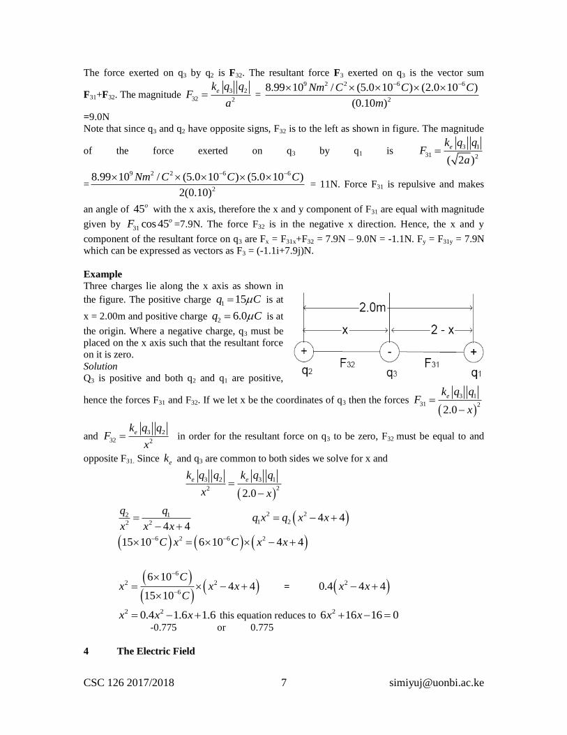
Example
Three charges lie along the x axis as shown in
the figure. The positive charge 1 15q C is at
x = 2.00m and positive charge 2 6.0q C is at
the origin. Where a negative charge, q3 must be
placed on the x axis such that the resultant force
on it is zero.
Solution
Q3 is positive and both q2 and q1 are positive,
hence the forces F31 and F32. If we let x be the coordinates of q3 then the forces
3 1
31 22.0
ek q qF
x
and 3 2
32 2
ek q qF
x in order for the resultant force on q3 to be zero, F32 must be equal to and
opposite F31. Since ek and q3 are common to both sides we solve for x and
3 2 3 1
222.0
e ek q q k q q
x x
2 1
2 2 4 4
q q
x x x
2 2
1 2 4 4q x q x x
6 2 6 215 10 6 10 4 4C x C x x
6
2 2
6
6 104 4
15 10
Cx x x
C
= 20.4 4 4x x
2 20.4 1.6 1.6x x x this equation reduces to
26 16 16 0x x
-0.775 or 0.775
4 The Electric Field
CSC 126 2017/2018 8 [email protected]
The electric field vector E at a point in space is defined as the electric force F acting on a positive
test charge placed at that point divided by the magnitude of the test charge qo.
oq
FE (1.4)
E is the field produced by some charge external to the test charge and not the field
produced by the test charge, E has unit N/C
Since the electric field at the position of the test charge is defined by
oq
FE we find that, at the
position of qo the electric charge by q is
2
ek q
rE r (1.4)
r is a unit vector directed from q towards qo
The total electric field due to a group of charges equals the vector sum of the electric
fields of all the charges e.g to calculate the electric field at point P due to a group of point
charges, first calculate electric field vectors at P individually using equation 1.5 then add
them vectorially.
Thus, the electric field of a group of charges (excluding the test charge qo) can be expressed as
2
ie
i i
qk
r E r (1.5)
ri is the distance from the ith charge to the point P (the location of the test charge) and ri is a unit
vector directed from qi towards P.
Example
Find the electric force on a proton placed in an electric field of 42.0 10 N/C directed along the positive x axis.
Solution
Charge of proton 191.6 10 Ce , the electric force on it is
F eE
19 4 151.6 10 2.0 10 / 3.2 10F C N C N
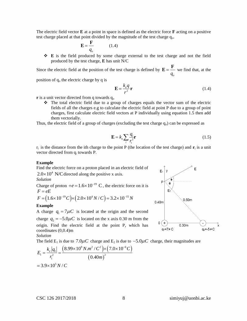
Example
A charge 1 7q C is located at the origin and the second
charge 2 5.0q C is located on the x axis 0.30 m from the
origin. Find the electric field at the point P, which has
coordinates (0,0.4)m
Solution
The field E1 is due to 7.0 C charge and E2 is due to 5.0 C charge, their magnitudes are
9 2 2 6
1
1 22
1
5
8.99 10 . / 7.0 10
0.40
3.9 10 /
eN m C Ck q
Er m
N C
CSC 126 2017/2018 9 [email protected]
2
9 2 2 6
2
2 2
2
5
8.99 10 . / 5.0 10
0.5
1.8 10 /
eN m C Ck q
Er m
N C
The vector E1 has only y component. The vector E2 has an x component given by
2 2
3cos
5 E E and negative y component given by
2
4sin sin
5 E . Hence the vectors
can be expressed as 5
1 3.9 10 /E jN C 5 5
2 1.1 10 1.4 10 /E i j N C . The resultant
field E at P is the superposition of E1 and E2, E = E1 + E2
5 51.1 10 2.46 10 /i j N C
E
E has the magnitude 2 2 51.1 2.46 2.69 10 /E N C and makes an angle of 66o
with positive x axis.
Electric Field Lines
The electric lines for a point charge
i. For a positive point charge, the lines are radially outward
ii. For a negative point charge, the lines are radially inwards
Rules for drawing electric field lines for any charge distribution
i. The lines must begin on positive charges and terminate on negative charges, although if the
net charge is not zero, the lines may begin or terminate at infinity
ii. The number of lines drawn leaving a positive charge or approaching a negative charge is
proportional to the magnitude of the charge
iii. No two field lines can cross or touch
5 Motion of Charged Particles in a Uniform Electric Field
When a particle of charge q and mass m is placed in an electric field E, the electric force exerted
on the charge is qE. If this is the only force exerted on the charge, then Newton’s second law
applied to the charge gives q ma F E , acceleration of the particle is therefore
qE
am
(1.6)
If E is uniform (that is constant in magnitude and direction) the acceleration is a constant of the
motion. If the charge is positive, the acceleration is in the direction of the electric field. If the
charge is negative the acceleration is in the direction opposite the electric field.
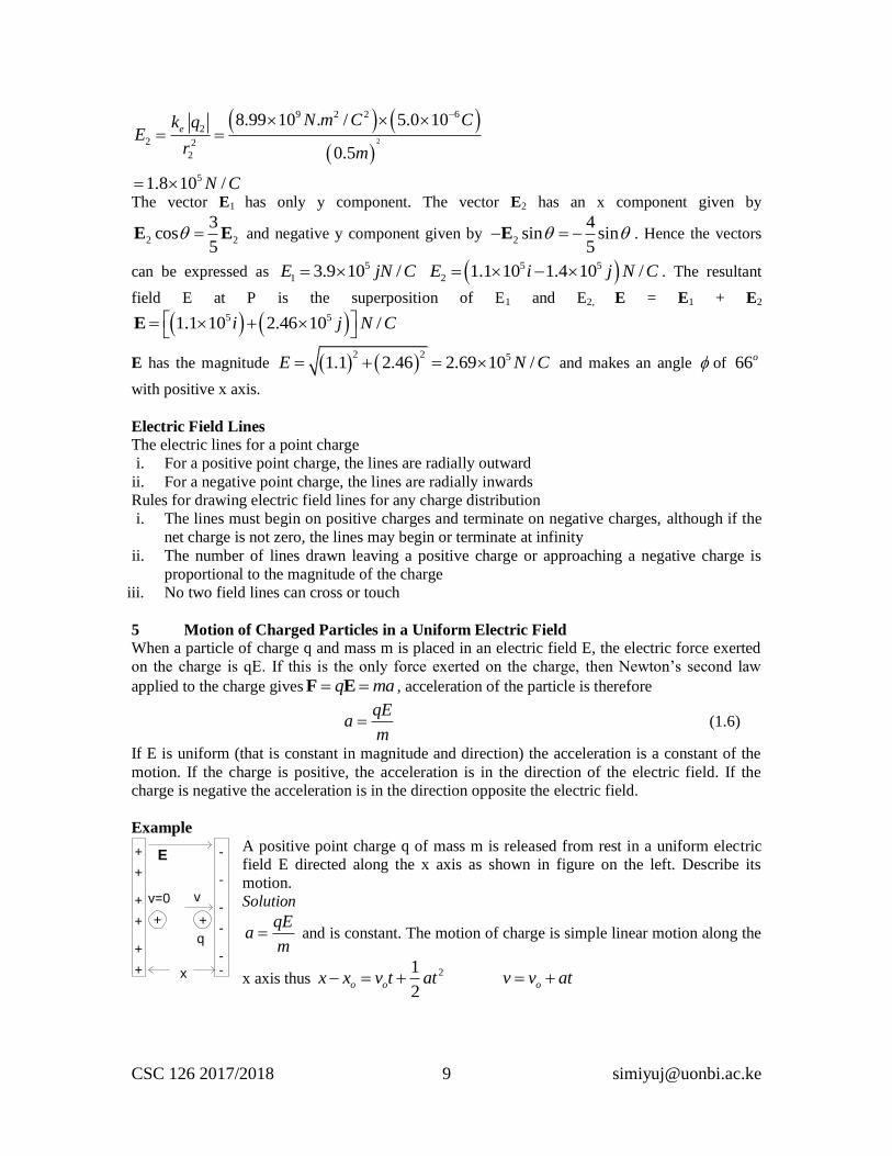
Example
A positive point charge q of mass m is released from rest in a uniform electric
field E directed along the x axis as shown in figure on the left. Describe its
motion.
Solution
qEa
m and is constant. The motion of charge is simple linear motion along the
x axis thus 21
2o o ox x v t at v v at
+
+
+
+
+
+
-
-
-
-
--x
vv=0
+ +
q
E
CSC 126 2017/2018 10 [email protected]
2 2 2 ( )o ov v a x x taking 0 and 0ox v gives 2 21
2 2
qEx at t
m but v at therefore
qE
v at tm
and 2 2
2qE
v ax xm
. The kinetic energy of the charge after it has
moved a distance x is 21 1 2
2 2
qEk mv m x qEx
m
.
6 Gauss Law
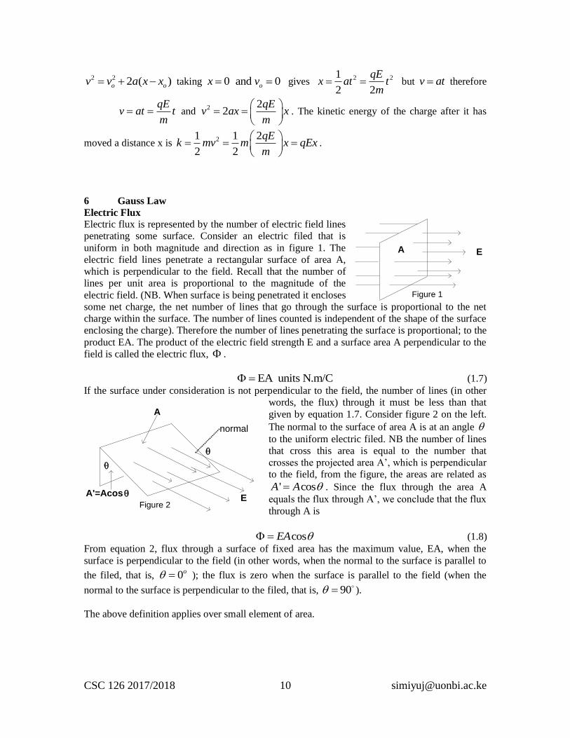
Electric Flux
Electric flux is represented by the number of electric field lines
penetrating some surface. Consider an electric filed that is
uniform in both magnitude and direction as in figure 1. The
electric field lines penetrate a rectangular surface of area A,
which is perpendicular to the field. Recall that the number of
lines per unit area is proportional to the magnitude of the
electric field. (NB. When surface is being penetrated it encloses
some net charge, the net number of lines that go through the surface is proportional to the net
charge within the surface. The number of lines counted is independent of the shape of the surface
enclosing the charge). Therefore the number of lines penetrating the surface is proportional; to the
product EA. The product of the electric field strength E and a surface area A perpendicular to the
field is called the electric flux, .
EA units N.m/C (1.7)
If the surface under consideration is not perpendicular to the field, the number of lines (in other
words, the flux) through it must be less than that
given by equation 1.7. Consider figure 2 on the left.
The normal to the surface of area A is at an angle
to the uniform electric filed. NB the number of lines
that cross this area is equal to the number that
crosses the projected area A’, which is perpendicular
to the field, from the figure, the areas are related as
' cosA A . Since the flux through the area A
equals the flux through A’, we conclude that the flux
through A is
cosEA (1.8)
From equation 2, flux through a surface of fixed area has the maximum value, EA, when the
surface is perpendicular to the field (in other words, when the normal to the surface is parallel to
the filed, that is, 0o ); the flux is zero when the surface is parallel to the field (when the
normal to the surface is perpendicular to the filed, that is, 90 ).
The above definition applies over small element of area.
EA
Figure 1
normal
E
A
A'=Acos
Figure 2
CSC 126 2017/2018 11 [email protected]
II Current and Resistance
1. Electric Current
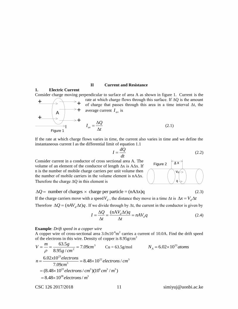
Consider charge moving perpendicular to surface of area A as shown in figure 1. Current is the
rate at which charge flows through this surface. If ΔQ is the amount
of charge that passes through this area in a time interval Δt, the
average current avI is
av
QI
t
(2.1)
If the rate at which charge flows varies in time, the current also varies in time and we define the
instantaneous current I as the differential limit of equation 1.1
dQ
Idt
(2.2)
Consider current in a conductor of cross sectional area A. The
volume of an element of the conductor of length Δx is AΔx. If
n is the number of mobile charge carriers per unit volume then
the number of mobile carriers in the volume element is nAΔx.
Therefore the charge ΔQ in this element is
number of charges charge per particle = (nA x)qQ (2.3)
If the charge carriers move with a speed dV , the distance they move in a time Δt is tVx d
Therefore qtnAVQ d )( . If we divide through by Δt, the current in the conductor is given by
(nA )d
d
V t qQI nAV q
t t
(2.4)
Example: Drift speed in a copper wire
A copper wire of cross-sectional area 3.0x10⁻⁶
m2 carries a current of 10.0A. Find the drift speed
of the electrons in this wire. Density of copper is 8.95g/cm2
3
209.7
/95.8
5.63cm
cmg
gmV
Cu = 63.5g/mol
236.02 10AN atoms
2322 3
3
6.02 108.48 10 /
7.09
x electronsn electrons cm
cm
22 3 6 3 3(8.48 10 / )(10 / )electrons cm cm m
28 38.48 10 /electrons m
+
+
++
+
A
IFigure 1
q
vd
xFigure 2
CSC 126 2017/2018 12 [email protected]
28 3 19 6 2
10.0 /
(8.48 10 ) (1.6 10 ) (3.0 10 )d
I C sV
nqA x m x C x m
42.46 10 /m s
2. Resistance and Ohm’s Law
Consider a conductor of cross sectional area A carrying current I. The current density J in the
conductor is defined to be the current per unit area. Since the current AnqVI d , the current
density is
2 units A/md
IJ nqV
A (2.5)
A current density J and an electric field E are established in a conductor when potential
difference is maintained across the conductor. If the potential difference is constant, the current is
also constant. Very often, the current density is proportional to the electric field and we express
J E (2.6)
Materials that obey equation 2.6 are said to follow Ohm’s law named after George Simon Ohm
(1787-1854). More specifically, Ohm’s law states that: the ratio of the current density to the
electric field is a constant, , that is independent of the electric field producing the current.
Materials that obey Ohm’s law and hence demonstrate this linear behavior between E and J are
said to be Ohmic. Potential difference is related to the electric field through the relationship
V lE where l is the distance of separation where electric field E is acting. Therefore
V
l J E (2.7)
Since J = I/A, the potential difference can be expressed as
l l
V IA
J (2.8)
The quantity l
Ais called the resistance R of the conductor, hence
units V/A=l V
RA I
(2.9)
The inverse of conductivity is resistivity
I
(2.10)
Hence
l
RA
(2.11)
Example: The resistance of a conductor
Calculate the resistance of an aluminum cylinder that is 10.0 cm long and has a cross sectional
area of 2.00x10⁻⁴
m2. Repeat the calculation for a glass cylinder of resistivity 3.0x10
10 m.
Solution
R 8 5
4 2
0.100(2.82 10 ) 1.41 10
2.00 10
l mm
A m
10 13
4 2
0.100(3.0 10 ) 1.5 10
2.00 10
l mR m
A m
CSC 126 2017/2018 13 [email protected]
Resistance varies with temperature if a wire has a resistance Ro at a temperature To then its
resistance R at a temperature T is
)( oooo TTRRR where α is the temperature coefficient of resistance of the
material of the wire and it varies with temperature and so its application is over short ranges.
Units K-1
or -1Co
A similar relation applies for resistivity
oT - To o
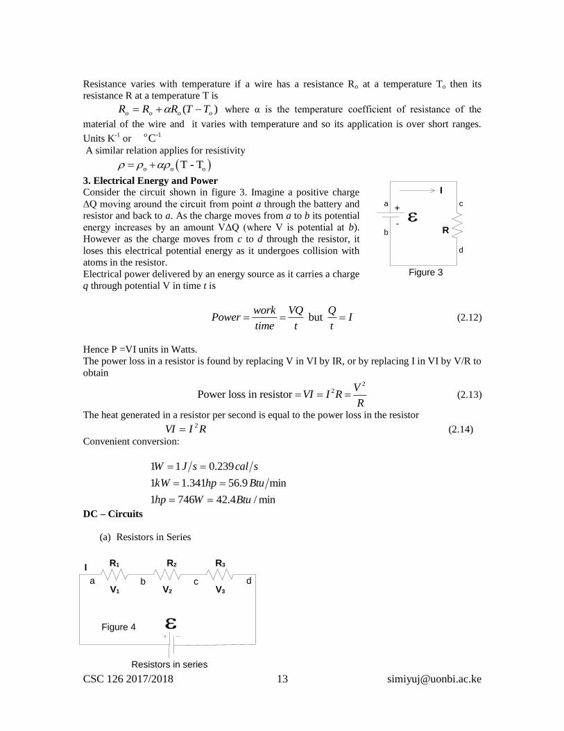
3. Electrical Energy and Power
Consider the circuit shown in figure 3. Imagine a positive charge
ΔQ moving around the circuit from point a through the battery and
resistor and back to a. As the charge moves from a to b its potential
energy increases by an amount VΔQ (where V is potential at b).
However as the charge moves from c to d through the resistor, it
loses this electrical potential energy as it undergoes collision with
atoms in the resistor.
Electrical power delivered by an energy source as it carries a charge
q through potential V in time t is
but work VQ Q
Power Itime t t
(2.12)
Hence P =VI units in Watts.
The power loss in a resistor is found by replacing V in VI by IR, or by replacing I in VI by V/R to
obtain
22Power loss in resistor
VVI I R
R (2.13)
The heat generated in a resistor per second is equal to the power loss in the resistor
RIVI 2 (2.14)
Convenient conversion:
min/4.427461
min9.56341.11
239.011
BtuWhp
BtuhpkW
scalsJW
DC – Circuits
(a) Resistors in Series
R
a
b
c
d
+
-
I
Figure 3
R1 R2 R3
V1 V2 V3
I
a b c d
Resistors in series
Figure 4
CSC 126 2017/2018 14 [email protected]
For resistors in series
1 2 3..........eq nR R R R R
ad ab bc cdV V V V
ab bc cdI I I I
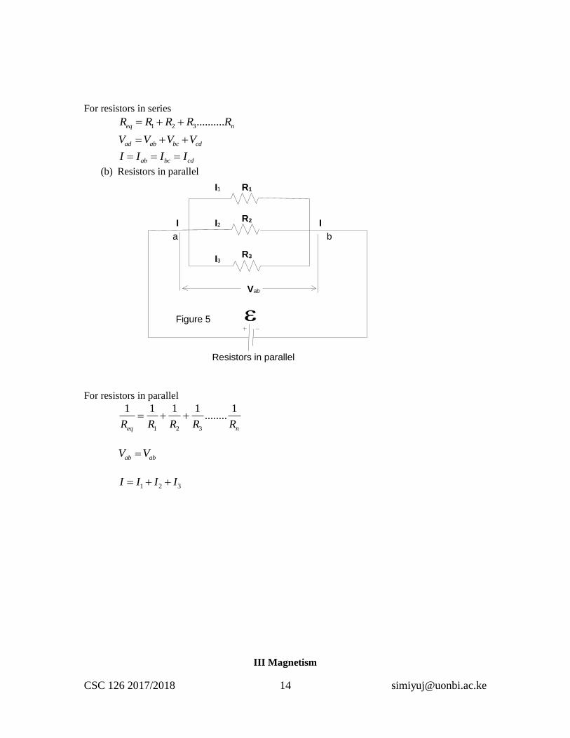
(b) Resistors in parallel
For resistors in parallel
1 2 3
1 1 1 1 1........
eq nR R R R R
ab abV V
1 2 3I I I I
III Magnetism
R1
R2
R3
I
a b
Resistors in parallel
Figure 5
I
Vab
I2
I1
I3
CSC 126 2017/2018 15 [email protected]
Metallic materials that attract ion filings have a property of magnetism and the materials are
called magnets. Magnetic materials have the following properties
1. Have two poles (north and south)
2. Like poles repel each other while unlike poles attract each other.
3. Magnetic material will rest freely in the north south orientation
Magnetism is used in storage media for computers.
1. Magnetic Fields
When a charged particle is moving through a magnetic field, a magnetic force acts on it. It is
found experimentally that the strength of the magnetic force F on the particle is proportional to
the magnitude of the charge q, the magnitude of the velocity v, the strength of the external
magnetic field B, and the sine of the angle θ between the direction of v and the direction of B. The
force is given by
(3.1)
This force has its maximum value when the charge moves in a direction perpendicular to the
magnetic field lines, decreases in value at other angles, and becomes zero when the particle
moves along the field lines. Further, the electric force is directed parallel to the electric field
while the magnetic force on a moving charge is directed perpendicular to the magnetic field.
If F is in newtons, q in coulombs, and v in meters per second, then the SI unit of magnetic field is
the tesla (T), also called the weber (Wb) per square meter (1 T = 1 Wb/m2. From the equation
above, it can be seen that the force on a charged particle moving in a magnetic field has its
maximum value when the particle’s motion is perpendicular to the magnetic field, corresponding
to θ = 90°, so that sin θ = 1. The magnitude of this maximum force has the value
Fmax = qvB (3.2)
Also F is zero when is parallel to (corresponding to θ = 0° or 180°), so no magnetic force is
exerted on a charged particle when it moves in the direction of the magnetic field or opposite the
field.
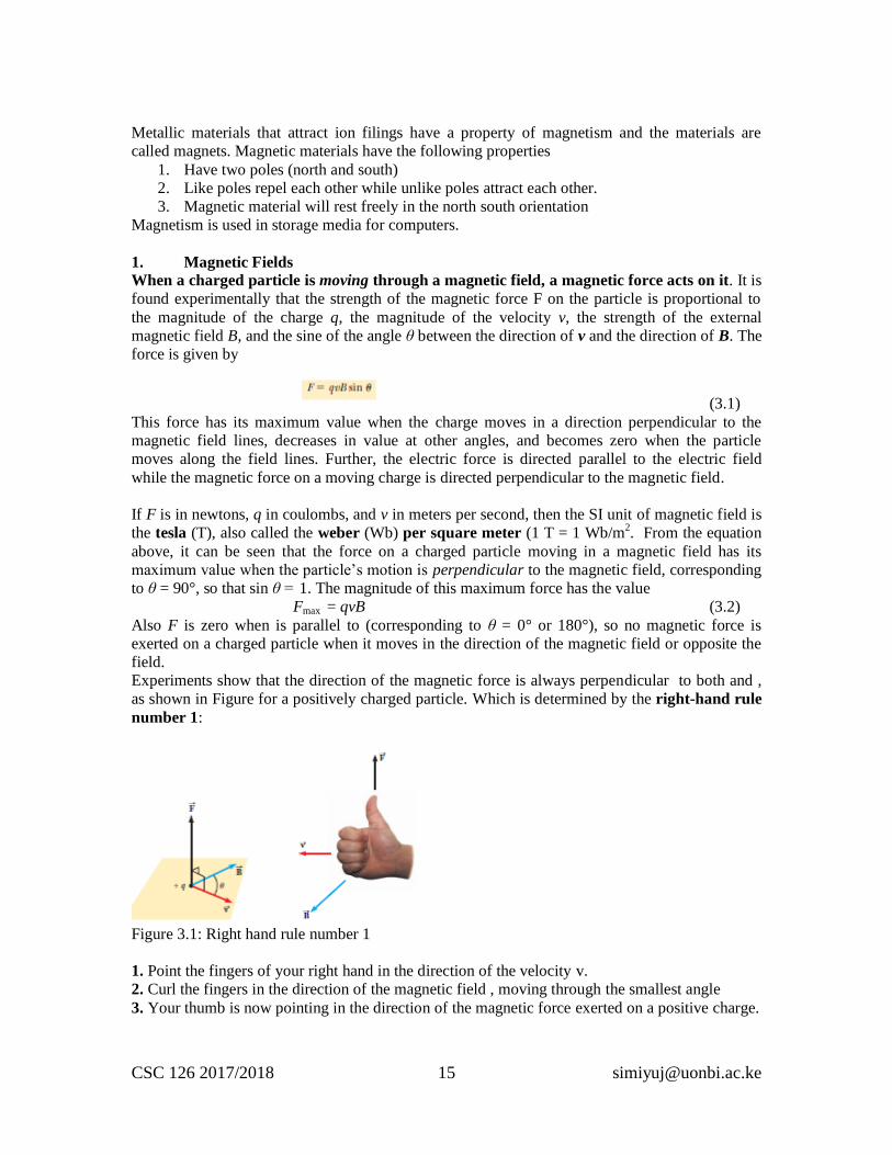
Experiments show that the direction of the magnetic force is always perpendicular to both and ,
as shown in Figure for a positively charged particle. Which is determined by the right-hand rule
number 1:
Figure 3.1: Right hand rule number 1
1. Point the fingers of your right hand in the direction of the velocity v.
2. Curl the fingers in the direction of the magnetic field , moving through the smallest angle
3. Your thumb is now pointing in the direction of the magnetic force exerted on a positive charge.
CSC 126 2017/2018 16 [email protected]
2. Magnetic Force on a Current-Carrying Conductor
If a magnetic field exerts a force on a single charged particle when it moves through a magnetic
field, it should be no surprise that magnetic forces are exerted on a current-carrying wire, as well.
This follows from the fact that the current is a collection of many charged particles in motion;
hence, the resultant force on the wire is due to the sum of the individual forces on the charged
particles. The force on the particles is transmitted to the ―bulk‖ of the wire through collisions with
the atoms making up the wire. Some explanation is in order concerning notation in many of the
figures.
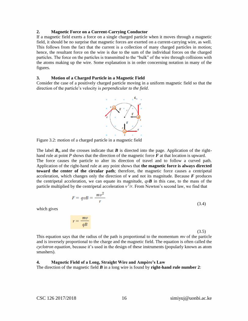
3. Motion of a Charged Particle in a Magnetic Field
Consider the case of a positively charged particle moving in a uniform magnetic field so that the
direction of the particle’s velocity is perpendicular to the field.
Figure 3.2: motion of a charged particle in a magnetic field
The label Bin and the crosses indicate that B is directed into the page. Application of the right-
hand rule at point P shows that the direction of the magnetic force F at that location is upward.
The force causes the particle to alter its direction of travel and to follow a curved path.
Application of the right-hand rule at any point shows that the magnetic force is always directed
toward the center of the circular path; therefore, the magnetic force causes a centripetal
acceleration, which changes only the direction of v and not its magnitude. Because F produces
the centripetal acceleration, we can equate its magnitude, qvB in this case, to the mass of the
particle multiplied by the centripetal acceleration v 2/r. From Newton’s second law, we find that
(3.4)
which gives
(3.5)
This equation says that the radius of the path is proportional to the momentum mv of the particle
and is inversely proportional to the charge and the magnetic field. The equation is often called the
cyclotron equation, because it’s used in the design of these instruments (popularly known as atom
smashers).
4. Magnetic Field of a Long, Straight Wire and Ampère’s Law
The direction of the magnetic field B in a long wire is found by right-hand rule number 2:
CSC 126 2017/2018 17 [email protected]
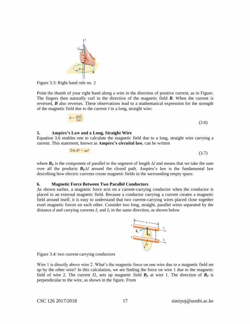
Figure 3.3: Right hand rule no. 2
Point the thumb of your right hand along a wire in the direction of positive current, as in Figure.
The fingers then naturally curl in the direction of the magnetic field B. When the current is
reversed, B also reverses. These observations lead to a mathematical expression for the strength
of the magnetic field due to the current I in a long, straight wire:
(3.6)
5. Ampère’s Law and a Long, Straight Wire
Equation 3.6 enables one to calculate the magnetic field due to a long, straight wire carrying a
current. This statement, known as Ampère’s circuital law, can be written
(3.7)
where BE is the component of parallel to the segment of length ∆l and means that we take the sum
over all the products BE∆l around the closed path. Ampère’s law is the fundamental law
describing how electric currents create magnetic fields in the surrounding empty space.
6. Magnetic Force Between Two Parallel Conductors
As shown earlier, a magnetic force acts on a current-carrying conductor when the conductor is
placed in an external magnetic field. Because a conductor carrying a current creates a magnetic
field around itself, it is easy to understand that two current-carrying wires placed close together
exert magnetic forces on each other. Consider two long, straight, parallel wires separated by the
distance d and carrying currents I1 and I2 in the same direction, as shown below
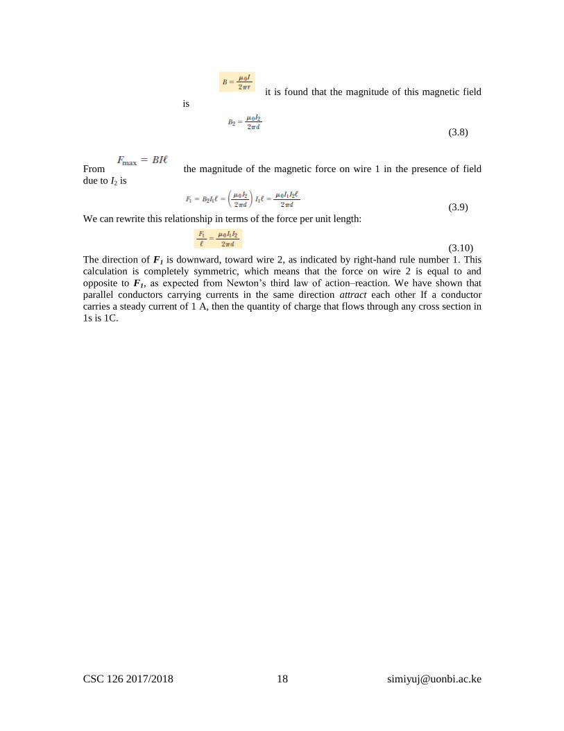
Figure 3.4: two current carrying conductors
Wire 1 is directly above wire 2. What’s the magnetic force on one wire due to a magnetic field set
up by the other wire? In this calculation, we are finding the force on wire 1 due to the magnetic
field of wire 2. The current I2, sets up magnetic field B2 at wire 1. The direction of B2 is
perpendicular to the wire, as shown in the figure. From
CSC 126 2017/2018 18 [email protected]
it is found that the magnitude of this magnetic field
is
(3.8)
From the magnitude of the magnetic force on wire 1 in the presence of field
due to I2 is
(3.9)
We can rewrite this relationship in terms of the force per unit length:
(3.10)
The direction of F1 is downward, toward wire 2, as indicated by right-hand rule number 1. This
calculation is completely symmetric, which means that the force on wire 2 is equal to and
opposite to F1, as expected from Newton’s third law of action–reaction. We have shown that
parallel conductors carrying currents in the same direction attract each other If a conductor
carries a steady current of 1 A, then the quantity of charge that flows through any cross section in
1s is 1C.
CSC 126 2017/2018 19 [email protected]
IV Alternating Current Circuits and Electromagnetic Waves
Introduction
Every time we turn on a television set, a stereo system, a pc or laptop or any of a multitude of
other electric appliances, we call on alternating currents (AC) to provide the power to operate
them. These equipments mentioned above have circuits that comprise among other items,
resistors, capacitors and inductors (these are known as the basic circuit devices). When these
devices encounter and ac supply, they behave differently under different conditions. We begin
our study of AC circuits by examining the characteristics of a circuit containing a source of power
and one other circuit element: a resistor, a capacitor, or an inductor. Then we examine what
happens when these elements are connected in combination with each other. The discussion is
limited to simple series configurations of the three kinds of elements. The section ends with a
discussion of electromagnetic waves, which are composed of fluctuating electric and magnetic
fields. Electromagnetic waves in the form of visible light enable us to view the world around us;
infrared waves warm our environment; radio-frequency waves carry our television and radio
programs, as well as information about processes in the core of our galaxy. X-rays allow us to
perceive structures hidden inside our bodies, and study properties of distant, collapsed stars.
1. Resistor Circuit
An AC circuit consists of combinations of circuit elements and an AC generator or an AC source,
which provides the alternating current. We have seen that the output of an AC generator is
sinusoidal and varies with time according to
(4.1)
where ∆v is the instantaneous voltage, ∆Vmax is the maximum voltage of the AC generator, and f
is the frequency at which the voltage changes, measured in hertz (Hz). Consider a simple circuit
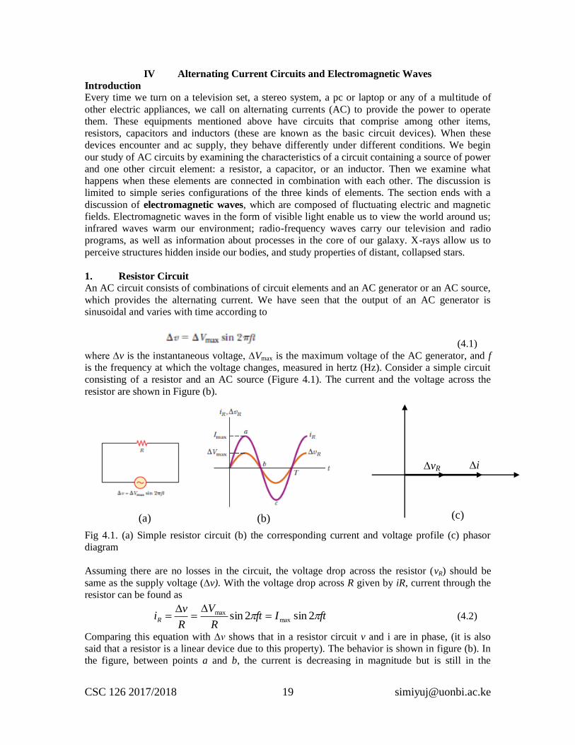
consisting of a resistor and an AC source (Figure 4.1). The current and the voltage across the
resistor are shown in Figure (b).
Fig 4.1. (a) Simple resistor circuit (b) the corresponding current and voltage profile (c) phasor
diagram
Assuming there are no losses in the circuit, the voltage drop across the resistor (vR) should be
same as the supply voltage (∆v). With the voltage drop across R given by iR, current through the
resistor can be found as
ftIftR
V
R
viR 2sin2sin max
max
(4.2)
Comparing this equation with ∆v shows that in a resistor circuit v and i are in phase, (it is also
said that a resistor is a linear device due to this property). The behavior is shown in figure (b). In
the figure, between points a and b, the current is decreasing in magnitude but is still in the
∆i
R
∆vR
(a) (b) (c)
CSC 126 2017/2018 20 [email protected]
positive direction. At point b, the current is momentarily zero; it then begins to increase in the
opposite (negative) direction between points b and c. At point c, the current has reached its
maximum value in the negative direction. The current and voltage are in step with each other
because they vary identically with time. Because the current and the voltage reach their
maximum values at the same time, they are said to be in phase.
2. Capacitor Circuit
Still the input voltage varies as
(4.3)
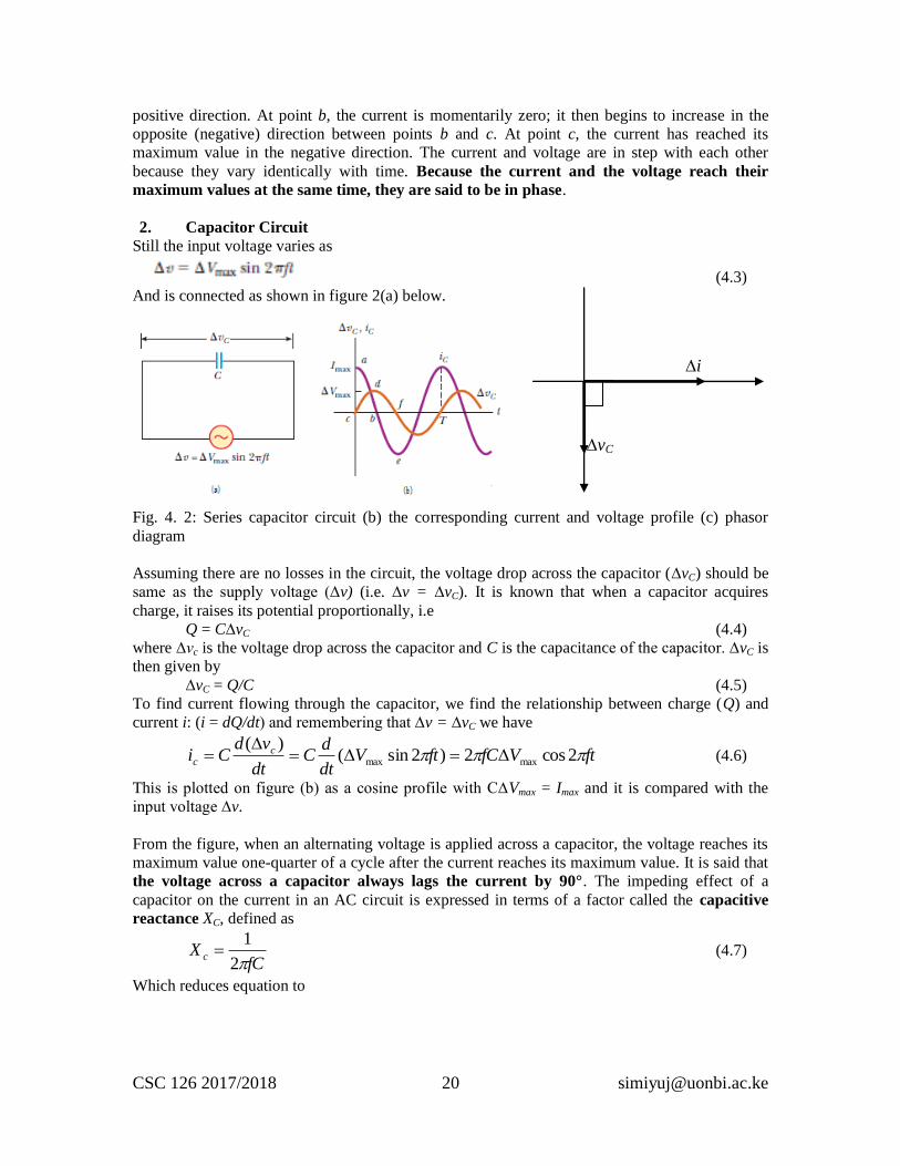
And is connected as shown in figure 2(a) below.
Fig. 4. 2: Series capacitor circuit (b) the corresponding current and voltage profile (c) phasor
diagram
Assuming there are no losses in the circuit, the voltage drop across the capacitor (∆vC) should be
same as the supply voltage (∆v) (i.e. ∆v = ∆vC). It is known that when a capacitor acquires
charge, it raises its potential proportionally, i.e
Q = C∆vC (4.4)
where ∆vc is the voltage drop across the capacitor and C is the capacitance of the capacitor. ∆vC is
then given by
∆vC = Q/C (4.5)
To find current flowing through the capacitor, we find the relationship between charge (Q) and
current i: (i = dQ/dt) and remembering that ∆v = ∆vC we have
ftVfCftVdt
dC
dt
vdCi c
c 2cos2)2sin()(
maxmax
(4.6)
This is plotted on figure (b) as a cosine profile with C∆Vmax = Imax and it is compared with the
input voltage ∆v.
From the figure, when an alternating voltage is applied across a capacitor, the voltage reaches its
maximum value one-quarter of a cycle after the current reaches its maximum value. It is said that
the voltage across a capacitor always lags the current by 90°. The impeding effect of a
capacitor on the current in an AC circuit is expressed in terms of a factor called the capacitive
reactance XC, defined as
fCX c
2
1 (4.7)
Which reduces equation to
∆i
C
∆vC
CSC 126 2017/2018 21 [email protected]
ftIftX
Vi
c
c 2cos2cos maxmax
(4.8)
This is similar to Ohm’s law for a resistor with a difference being the capacitative reactance being
equivalent to resistance in the resistor circuit.
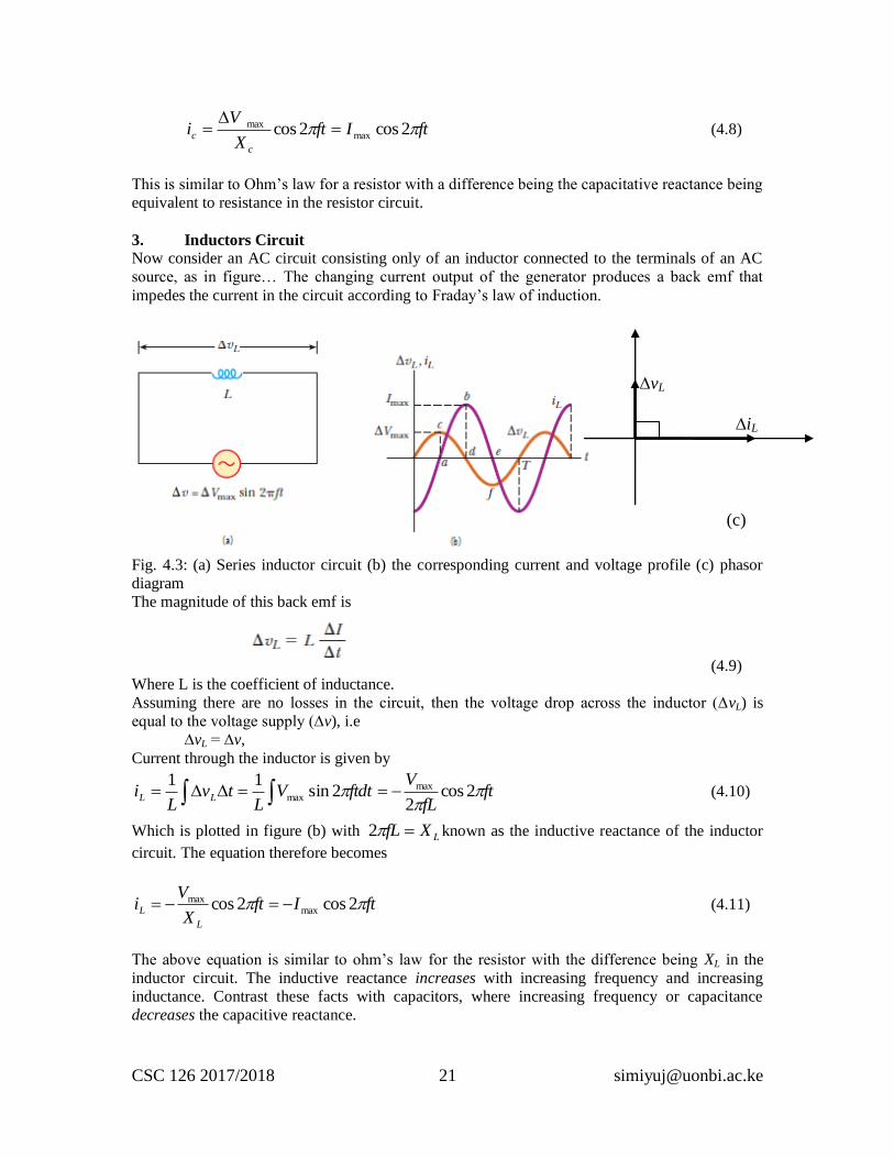
3. Inductors Circuit
Now consider an AC circuit consisting only of an inductor connected to the terminals of an AC
source, as in figure… The changing current output of the generator produces a back emf that
impedes the current in the circuit according to Fraday’s law of induction.
Fig. 4.3: (a) Series inductor circuit (b) the corresponding current and voltage profile (c) phasor
diagram
The magnitude of this back emf is
(4.9)
Where L is the coefficient of inductance.
Assuming there are no losses in the circuit, then the voltage drop across the inductor (∆vL) is
equal to the voltage supply (∆v), i.e
∆vL = ∆v,
Current through the inductor is given by
ftfL
VftdtV
Ltv
Li LL
2cos
22sin
11 maxmax (4.10)
Which is plotted in figure (b) with LXfL 2 known as the inductive reactance of the inductor
circuit. The equation therefore becomes
ftIftX
Vi
L
L 2cos2cos maxmax (4.11)
The above equation is similar to ohm’s law for the resistor with the difference being XL in the
inductor circuit. The inductive reactance increases with increasing frequency and increasing
inductance. Contrast these facts with capacitors, where increasing frequency or capacitance
decreases the capacitive reactance.
∆iL
∆vL
(c)
CSC 126 2017/2018 22 [email protected]
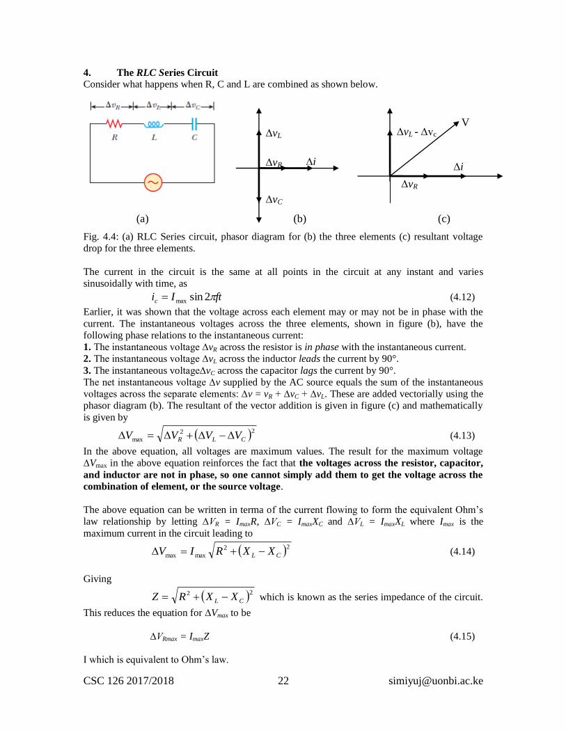
4. The RLC Series Circuit
Consider what happens when R, C and L are combined as shown below.
Fig. 4.4: (a) RLC Series circuit, phasor diagram for (b) the three elements (c) resultant voltage
drop for the three elements.
The current in the circuit is the same at all points in the circuit at any instant and varies
sinusoidally with time, as
ftIic 2sinmax (4.12)
Earlier, it was shown that the voltage across each element may or may not be in phase with the
current. The instantaneous voltages across the three elements, shown in figure (b), have the
following phase relations to the instantaneous current:
1. The instantaneous voltage ∆vR across the resistor is in phase with the instantaneous current.
2. The instantaneous voltage ∆vL across the inductor leads the current by 90°.
3. The instantaneous voltage∆vC across the capacitor lags the current by 90°.
The net instantaneous voltage ∆v supplied by the AC source equals the sum of the instantaneous
voltages across the separate elements: ∆v = vR + ∆vC + ∆vL. These are added vectorially using the
phasor diagram (b). The resultant of the vector addition is given in figure (c) and mathematically
is given by
22
max CLR VVVV (4.13)
In the above equation, all voltages are maximum values. The result for the maximum voltage
∆Vmax in the above equation reinforces the fact that the voltages across the resistor, capacitor,
and inductor are not in phase, so one cannot simply add them to get the voltage across the
combination of element, or the source voltage.
The above equation can be written in terma of the current flowing to form the equivalent Ohm’s
law relationship by letting ∆VR = ImaxR, ∆VC = ImaxXC and ∆VL = ImaxXL where Imax is the
maximum current in the circuit leading to
22
maxmax CL XXRIV (4.14)
Giving
22
CL XXRZ which is known as the series impedance of the circuit.
This reduces the equation for ∆Vmax to be
∆VRmax = ImaxZ (4.15)
I which is equivalent to Ohm’s law.
V
∆vR
∆vL - ∆vc
∆i ∆vR
∆vL
∆vC
∆i
(a) (b) (c)
CSC 126 2017/2018 23 [email protected]
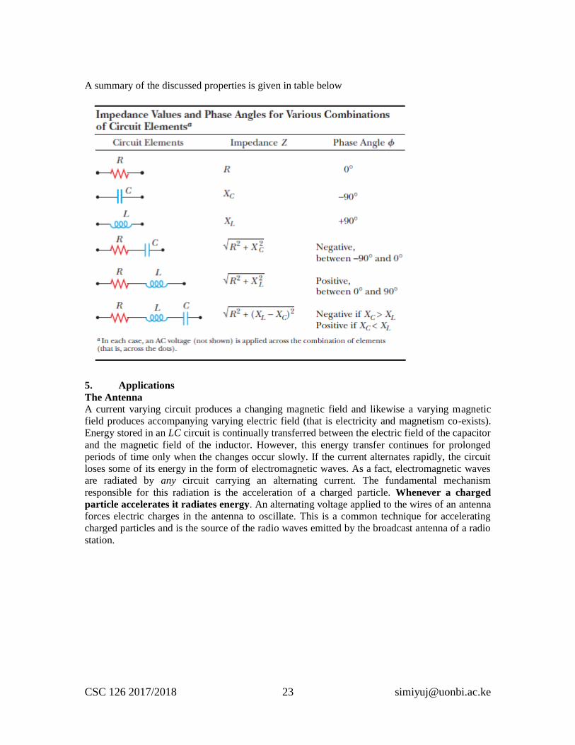
A summary of the discussed properties is given in table below
5. Applications
The Antenna
A current varying circuit produces a changing magnetic field and likewise a varying magnetic
field produces accompanying varying electric field (that is electricity and magnetism co-exists).
Energy stored in an LC circuit is continually transferred between the electric field of the capacitor
and the magnetic field of the inductor. However, this energy transfer continues for prolonged
periods of time only when the changes occur slowly. If the current alternates rapidly, the circuit
loses some of its energy in the form of electromagnetic waves. As a fact, electromagnetic waves
are radiated by any circuit carrying an alternating current. The fundamental mechanism
responsible for this radiation is the acceleration of a charged particle. Whenever a charged
particle accelerates it radiates energy. An alternating voltage applied to the wires of an antenna
forces electric charges in the antenna to oscillate. This is a common technique for accelerating
charged particles and is the source of the radio waves emitted by the broadcast antenna of a radio
station.
CSC 126 2017/2018 24 [email protected]
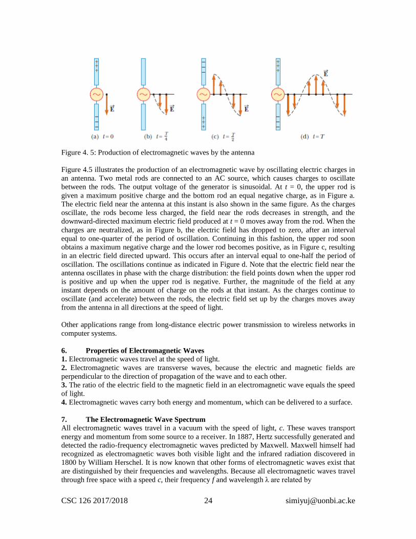
Figure 4. 5: Production of electromagnetic waves by the antenna
Figure 4.5 illustrates the production of an electromagnetic wave by oscillating electric charges in
an antenna. Two metal rods are connected to an AC source, which causes charges to oscillate
between the rods. The output voltage of the generator is sinusoidal. At t = 0, the upper rod is
given a maximum positive charge and the bottom rod an equal negative charge, as in Figure a.
The electric field near the antenna at this instant is also shown in the same figure. As the charges
oscillate, the rods become less charged, the field near the rods decreases in strength, and the
downward-directed maximum electric field produced at t = 0 moves away from the rod. When the
charges are neutralized, as in Figure b, the electric field has dropped to zero, after an interval
equal to one-quarter of the period of oscillation. Continuing in this fashion, the upper rod soon
obtains a maximum negative charge and the lower rod becomes positive, as in Figure c, resulting
in an electric field directed upward. This occurs after an interval equal to one-half the period of
oscillation. The oscillations continue as indicated in Figure d. Note that the electric field near the
antenna oscillates in phase with the charge distribution: the field points down when the upper rod
is positive and up when the upper rod is negative. Further, the magnitude of the field at any
instant depends on the amount of charge on the rods at that instant. As the charges continue to
oscillate (and accelerate) between the rods, the electric field set up by the charges moves away
from the antenna in all directions at the speed of light.
Other applications range from long-distance electric power transmission to wireless networks in
computer systems.
6. Properties of Electromagnetic Waves
1. Electromagnetic waves travel at the speed of light.
2. Electromagnetic waves are transverse waves, because the electric and magnetic fields are
perpendicular to the direction of propagation of the wave and to each other.
3. The ratio of the electric field to the magnetic field in an electromagnetic wave equals the speed
of light.
4. Electromagnetic waves carry both energy and momentum, which can be delivered to a surface.
7. The Electromagnetic Wave Spectrum
All electromagnetic waves travel in a vacuum with the speed of light, c. These waves transport
energy and momentum from some source to a receiver. In 1887, Hertz successfully generated and
detected the radio-frequency electromagnetic waves predicted by Maxwell. Maxwell himself had
recognized as electromagnetic waves both visible light and the infrared radiation discovered in
1800 by William Herschel. It is now known that other forms of electromagnetic waves exist that
are distinguished by their frequencies and wavelengths. Because all electromagnetic waves travel
through free space with a speed c, their frequency f and wavelength λ are related by
CSC 126 2017/2018 25 [email protected]
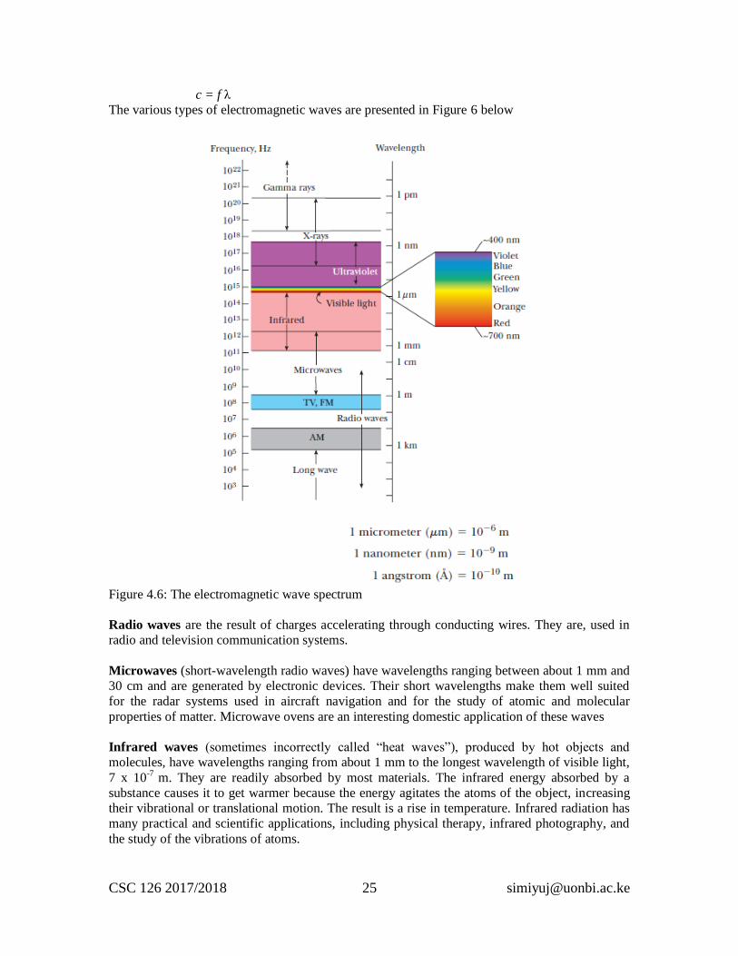
c = f λ
The various types of electromagnetic waves are presented in Figure 6 below
Figure 4.6: The electromagnetic wave spectrum
Radio waves are the result of charges accelerating through conducting wires. They are, used in
radio and television communication systems.
Microwaves (short-wavelength radio waves) have wavelengths ranging between about 1 mm and
30 cm and are generated by electronic devices. Their short wavelengths make them well suited
for the radar systems used in aircraft navigation and for the study of atomic and molecular
properties of matter. Microwave ovens are an interesting domestic application of these waves
Infrared waves (sometimes incorrectly called ―heat waves‖), produced by hot objects and
molecules, have wavelengths ranging from about 1 mm to the longest wavelength of visible light,
7 x 10⁻⁷
m. They are readily absorbed by most materials. The infrared energy absorbed by a
substance causes it to get warmer because the energy agitates the atoms of the object, increasing
their vibrational or translational motion. The result is a rise in temperature. Infrared radiation has
many practical and scientific applications, including physical therapy, infrared photography, and
the study of the vibrations of atoms.
CSC 126 2017/2018 26 [email protected]
Visible light, the most familiar form of electromagnetic waves, may be defined as the part of the
spectrum that is detected by the human eye. Light is produced by the rearrangement of electrons
in atoms and molecules. The wavelengths of visible light are classified as colors ranging from
violet λ ~ 4 x 10⁻⁷
m) to red (λ ~ 7 x 10⁻⁷
m). The eye’s sensitivity is a function of wavelength and
is greatest at a wavelength of about 5 .6 x 10-7
m (yellow green).
Ultraviolet (UV) light covers wavelengths ranging from about 4 x 10⁻⁷
m (400 nm) down to 6 x
10-10
m (0.6 nm). The Sun is an important source of ultraviolet light (which is the main cause of
suntans).
X-rays are electromagnetic waves with wavelengths from about 10-8
m (10 nm) down to 10-13
m
(10-4
nm). The most common source of x-rays is the acceleration of high-energy electrons
bombarding a metal target. X-rays are used as a diagnostic tool in medicine and as a treatment for
certain forms of cancer.
Gamma rays—electromagnetic waves emitted by radioactive nuclei—have wavelengths ranging
from about 10-10
m to less than 10-14
m. They are highly penetrating and cause serious damage
when absorbed by living tissues. Accordingly, those working near such radiation must be
protected by garments containing heavily absorbing materials, such as layers of lead. When
astronomers observe the same celestial object using detectors sensitive to different regions of the
electromagnetic spectrum, striking variations in the object’s features can be seen.
8. The Doppler Effect in Electromagnetic Waves
Doppler Effect is a phenomenon of apparent frequency of a wave observed when there is a
relative motion between the source of the wave and the observer. It is a phenomena that occurs
commonly in sound waves but it is also observed in electromagnetic waves. In Doppler effect, the
observed frequency of the wave is larger or smaller than the frequency emitted by the source of
the wave. Doppler Effect occurring in electromagnetic waves differs from that for sound waves in
two ways. First, in the case for sound waves, motion relative to the medium is most important,
because sound waves require a medium in which to propagate. In contrast, the medium of
propagation plays no role in the case for electromagnetic waves, because the waves require no
medium in which to propagate. Second, the speed of sound that appears in the equation for the
Doppler effect for sound depends on the reference frame in which it is measured. In contrast, the
speed of electromagnetic waves has the same value in all coordinate systems that are either at rest
or moving at constant velocity with respect to one another.
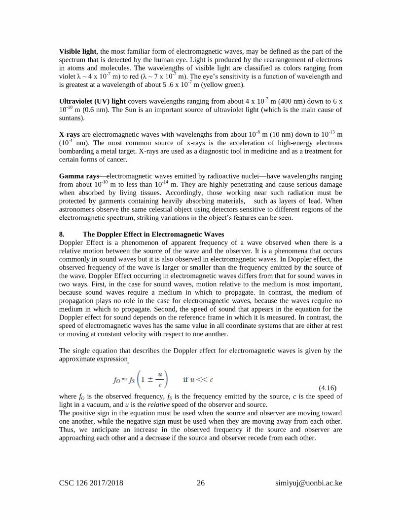
The single equation that describes the Doppler effect for electromagnetic waves is given by the
approximate expression
(4.16)
where fO is the observed frequency, fS is the frequency emitted by the source, c is the speed of
light in a vacuum, and u is the relative speed of the observer and source.
The positive sign in the equation must be used when the source and observer are moving toward
one another, while the negative sign must be used when they are moving away from each other.
Thus, we anticipate an increase in the observed frequency if the source and observer are
approaching each other and a decrease if the source and observer recede from each other.
CSC 126 2017/2018 27 [email protected]
V Wave Theory
Introduction
Wave motion is a form of disturbance that travels through the medium due to the repeated
periodic motion of particles of the medium about their mean positions. This disturbance is
transferred from one particle to the next, e.g water waves, sound. This also involves the transfer
of energy from one point to the other.
Characteristics of a wave
1. It’s a disturbance produced in the medium by repeated periodic motion of the particles of
the medium.
2. The wave travels forward while particles of the medium vibrate about their mean
positions
3. there is a regular phase change between various particles of the medium
4. Velocity of the wave is different from the velocity with which the particles of the
medium are vibrating about their mean positions.
Types of wave motion
1. Transverse wave: particles of the medium vibrate about their mean positions in the
direction perpendicular to the direction of propagation, e.g. light waves, water waves
etc
2. Longitudinal: particles of the medium vibrate about their mean position in the
direction of the wave, e.g sound wave
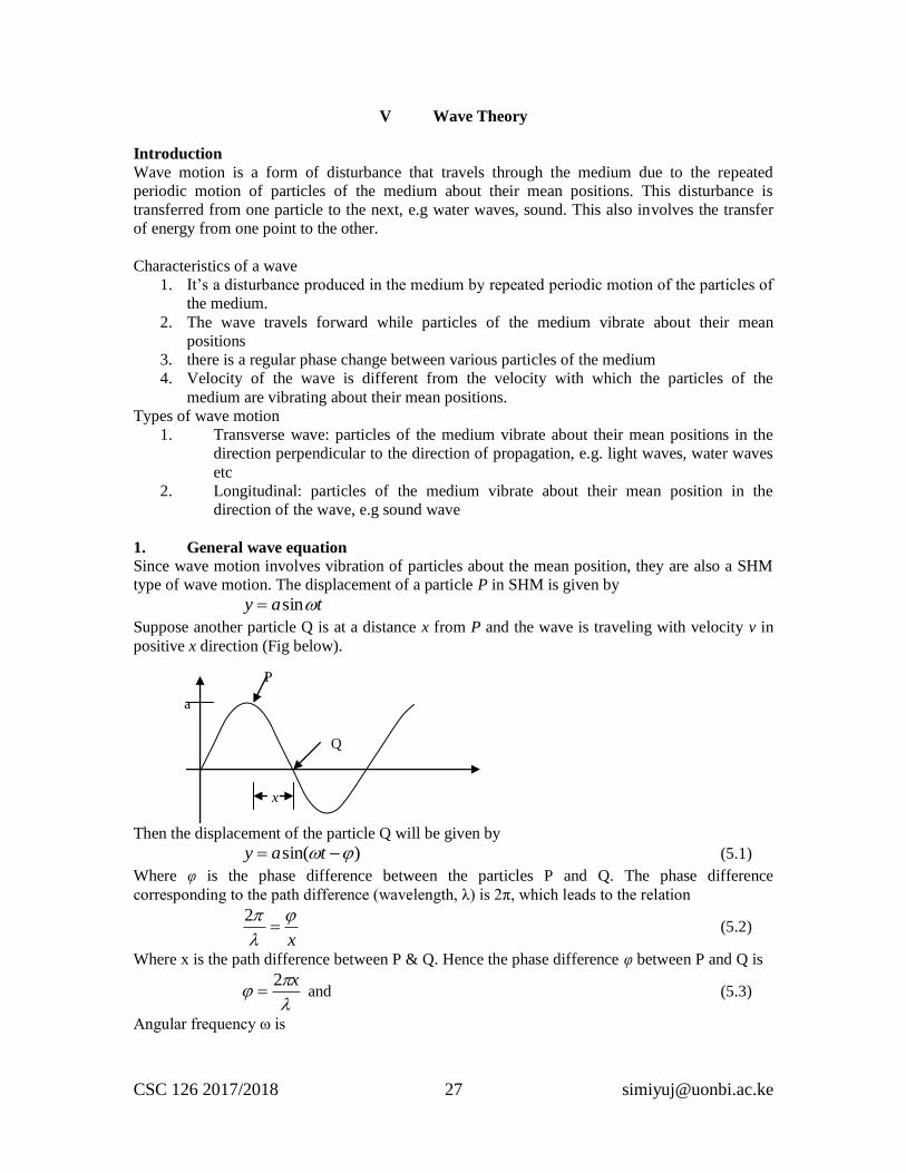
1. General wave equation
Since wave motion involves vibration of particles about the mean position, they are also a SHM
type of wave motion. The displacement of a particle P in SHM is given by
tay sin
Suppose another particle Q is at a distance x from P and the wave is traveling with velocity v in
positive x direction (Fig below).
Then the displacement of the particle Q will be given by
)sin( tay (5.1)
Where φ is the phase difference between the particles P and Q. The phase difference
corresponding to the path difference (wavelength, λ) is 2π, which leads to the relation
x
2 (5.2)
Where x is the path difference between P & Q. Hence the phase difference φ between P and Q is
x2 and (5.3)
Angular frequency ω is
P
Q
x
a
CSC 126 2017/2018 28 [email protected]
v
Tf
222 (5.4)
Hence equation (5.1) becomes
)22
sin(
xt
vay (5.5)
Or
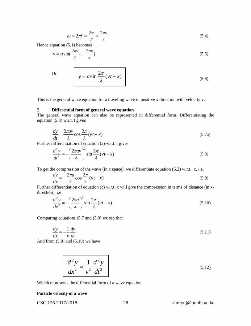
(5.6)
This is the general wave equation for a traveling wave in positive x direction with velocity v.
2. Differential form of general wave equation
The general wave equation can also be represented in differential form. Differentiating the
equation (5.3) w.r.t. t gives
)(2
cos2
xvtav
dt
dy
(5.7a)
Further differentiation of equation (a) w.r.t. t gives
)(2
sin2
2
2
2
xvtav
dt
yd
(5.8)
To get the compression of the wave (in x space), we differentiate equation (5.2) w.r.t. x, i.e.
)(2
cos2
xvta
dx
dy
(5.9)
Further differentiation of equation (c) w.r.t. x will give the compression in terms of distance (in x-
direction), i.e
)(2
sin2
2
2
2
xvta
dx
yd
(5.10)
Comparing equations (5.7 and (5.9) we see that
dt
dy
vdx
dy 1 (5.11)
And from (5.8) and (5.10) we have
(5.12)
Which represents the differential form of a wave equation.
Particle velocity of a wave
)(2
sin xvtay
2
2
22
2 1
dt
yd
vdx
yd
CSC 126 2017/2018 29 [email protected]
If the velocity of a particle is denoted by u then
)(2
cos2
xvtav
dt
dyu
(5.13)
And va
u
2max , which implies that
Maximum particle velocity is 2πa/λ times the wave velocity (v).
Likewise maximum particle acceleration is given by
av
f
2
max
2
(Show this)
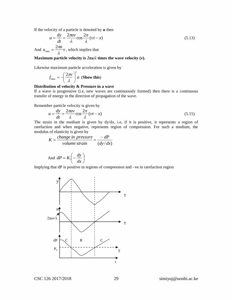
Distribution of velocity & Pressure in a wave
If a wave is progressive (i.e, new waves are continuously formed) then there is a continuous
transfer of energy in the direction of propagation of the wave.
Remember particle velocity is given by
)(2
cos2
xvtav
dt
dyu
(5.15)
The strain in the medium is given by dy/dx, i.e, if it is positive, it represents a region of
rarefaction and when negative, represents region of compression. For such a medium, the
modulus of elasticity is given by
)/( dxdy
dP
strainvolume
pressureinchangeK
And
dx
dyKdP .
Implying that dP is positive in regions of compression and –ve in rarefaction region
y
T
T
T
u
dP
t
Po
C R C
2πav/λ
CSC 126 2017/2018 30 [email protected]
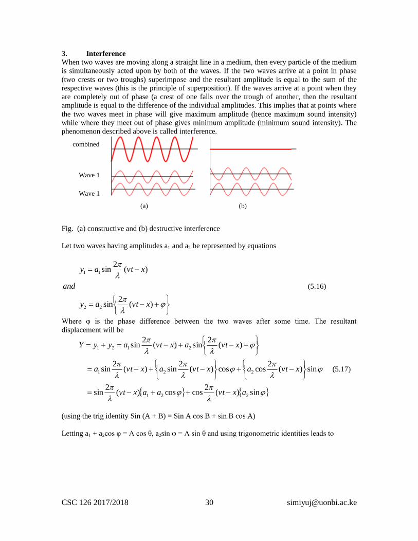
3. Interference
When two waves are moving along a straight line in a medium, then every particle of the medium
is simultaneously acted upon by both of the waves. If the two waves arrive at a point in phase
(two crests or two troughs) superimpose and the resultant amplitude is equal to the sum of the
respective waves (this is the principle of superposition). If the waves arrive at a point when they
are completely out of phase (a crest of one falls over the trough of another, then the resultant
amplitude is equal to the difference of the individual amplitudes. This implies that at points where
the two waves meet in phase will give maximum amplitude (hence maximum sound intensity)
while where they meet out of phase gives minimum amplitude (minimum sound intensity). The
phenomenon described above is called interference.
Fig. (a) constructive and (b) destructive interference
Let two waves having amplitudes a1 and a2 be represented by equations
)(2
sin
)(2
sin
22
11
xvtay
and
xvtay
(5.16)
Where φ is the phase difference between the two waves after some time. The resultant
displacement will be
sin)(2
coscos)(2
sin
sin)(2
coscos)(2
sin)(2
sin
)(2
sin)(2
sin
221
221
2121
axvtaaxvt
xvtaxvtaxvta
xvtaxvtayyY
(5.17)
(using the trig identity Sin (A + B) = Sin A cos B + sin B cos A)
Letting a1 + a2cos φ = A cos θ, a2sin φ = A sin θ and using trigonometric identities leads to
combined
Wave 1
Wave 1
(a) (b)
CSC 126 2017/2018 31 [email protected]
)(2
sin
)(2
cossin)(2
sincos
xvtAY
xvtAxvtAY
(5.18)
This shows that the resultant wave has the same frequency but a different amplitude and phase
from the component wave trains.
Special cases:
1. when φ = 0, A = a1 + a2 and hence tan θ = 0 showing that the resultant is in phase
with the component
2. when φ = 180o, A = a1 – a2
From 1 and 2 above, it implies that when the phase difference between two waves is zero the
two waves reinforce each other. This also implies that the resultant has the same period and
its amplitude is the sum of the amplitudes of the component waves. However, if the two
waves have a phase difference of 180o, they destroy each other and the resultant amplitude is
the difference between the amplitudes of the component waves.
Conditions for interference of waves
1. the two wave trains must move in the same direction.
2. The two sources must give waves of same frequency and amplitude so that the positions
of maxima and minima are distinct
3. the two sources must be in phase, i.e must be coherent source
CSC 126 2017/2018 32 [email protected]
VI Nature of Light
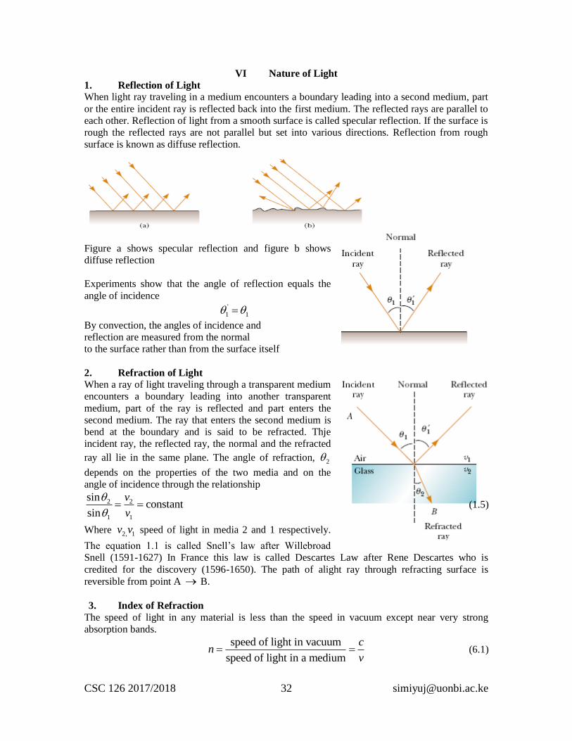
1. Reflection of Light
When light ray traveling in a medium encounters a boundary leading into a second medium, part
or the entire incident ray is reflected back into the first medium. The reflected rays are parallel to
each other. Reflection of light from a smooth surface is called specular reflection. If the surface is
rough the reflected rays are not parallel but set into various directions. Reflection from rough
surface is known as diffuse reflection.
Figure a shows specular reflection and figure b shows
diffuse reflection
Experiments show that the angle of reflection equals the
angle of incidence
'
1 1
By convection, the angles of incidence and
reflection are measured from the normal
to the surface rather than from the surface itself
2. Refraction of Light
When a ray of light traveling through a transparent medium
encounters a boundary leading into another transparent
medium, part of the ray is reflected and part enters the
second medium. The ray that enters the second medium is
bend at the boundary and is said to be refracted. Thje
incident ray, the reflected ray, the normal and the refracted
ray all lie in the same plane. The angle of refraction, 2
depends on the properties of the two media and on the
angle of incidence through the relationship
2 2
1 1
sinconstant
sin
v
v
(1.5)
Where 2, 1v v speed of light in media 2 and 1 respectively.
The equation 1.1 is called Snell’s law after Willebroad
Snell (1591-1627) In France this law is called Descartes Law after Rene Descartes who is
credited for the discovery (1596-1650). The path of alight ray through refracting surface is
reversible from point A B.
3. Index of Refraction
The speed of light in any material is less than the speed in vacuum except near very strong
absorption bands.
speed of light in vacuum
speed of light in a medium
cn
v (6.1)
CSC 126 2017/2018 33 [email protected]
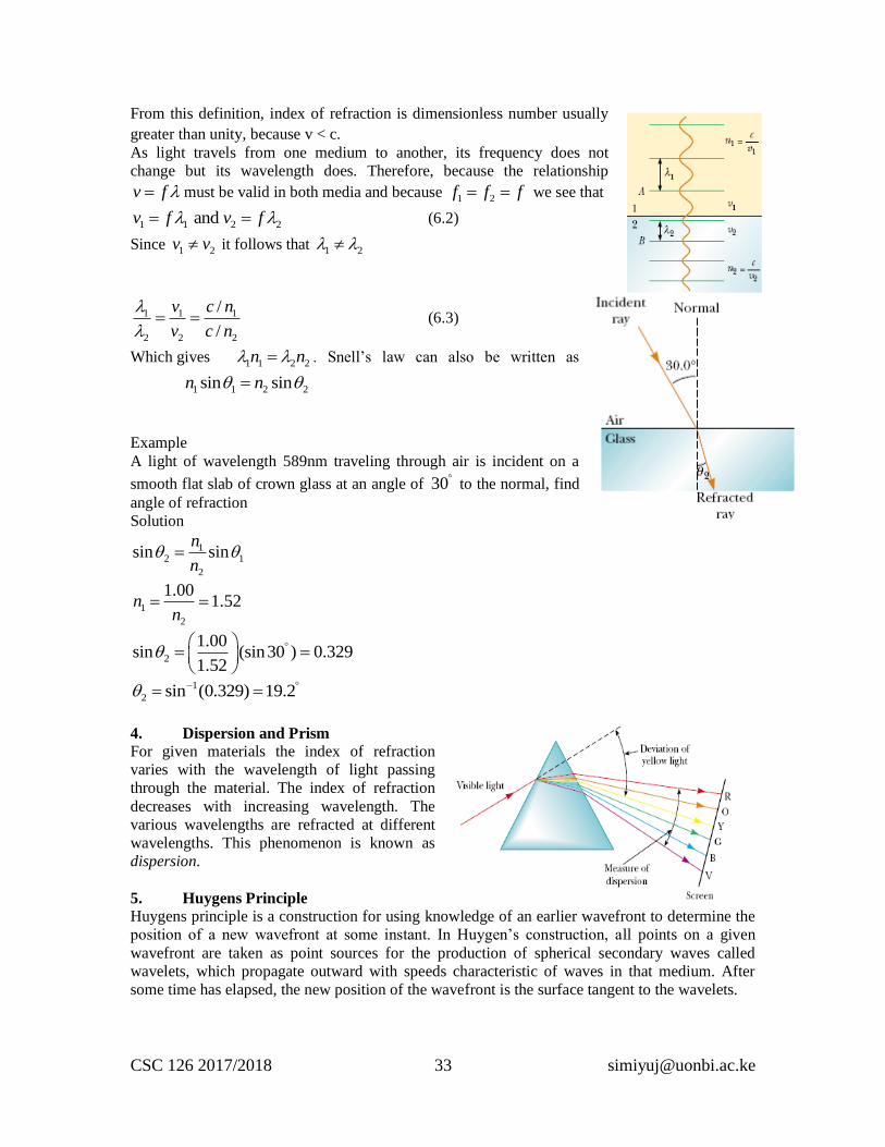
From this definition, index of refraction is dimensionless number usually
greater than unity, because v < c.
As light travels from one medium to another, its frequency does not
change but its wavelength does. Therefore, because the relationship
v f must be valid in both media and because 1 2f f f we see that
1 1 2 2 and v f v f (6.2)
Since 1 2v v it follows that 1 2
1 1 1
2 2 2
/
/
v c n
v c n
(6.3)
Which gives 1 1 2 2n n . Snell’s law can also be written as
1 1 2 2sin sinn n
Example
A light of wavelength 589nm traveling through air is incident on a
smooth flat slab of crown glass at an angle of 30 to the normal, find
angle of refraction
Solution
12 1
2
sin sinn
n
1
2
1.001.52n
n
2
1.00sin (sin30 ) 0.329
1.52
1
2 sin (0.329) 19.2
4. Dispersion and Prism
For given materials the index of refraction
varies with the wavelength of light passing
through the material. The index of refraction
decreases with increasing wavelength. The
various wavelengths are refracted at different
wavelengths. This phenomenon is known as
dispersion.
5. Huygens Principle
Huygens principle is a construction for using knowledge of an earlier wavefront to determine the
position of a new wavefront at some instant. In Huygen’s construction, all points on a given
wavefront are taken as point sources for the production of spherical secondary waves called
wavelets, which propagate outward with speeds characteristic of waves in that medium. After
some time has elapsed, the new position of the wavefront is the surface tangent to the wavelets.
CSC 126 2017/2018 34 [email protected]
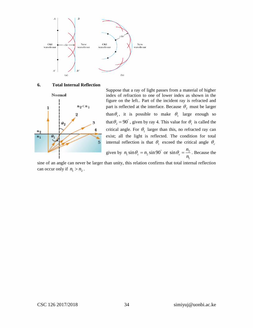
6. Total Internal Reflection
Suppose that a ray of light passes from a material of higher
index of refraction to one of lower index as shown in the
figure on the left.. Part of the incident ray is refracted and
part is reflected at the interface. Because 2 must be larger
than 1 , it is possible to make 1 large enough so
that 2 90 , given by ray 4. This value for 1 is called the
critical angle. For 1 larger than this, no refracted ray can
exist; all the light is reflected. The condition for total
internal reflection is that 1 exceed the critical angle c
given by 21 2
1
sin sin90 or sinc c
nn n
n . Because the
sine of an angle can never be larger than unity, this relation confirms that total internal reflection
can occur only if 1 2n n .