Recurrent Neural Networks

Instructor: Yoav Artzi

CS5740: Natural Language ProcessingSpring 2017

Adapted from Yoav Goldberg’s Book and slides by Sasha Rush

Overview• Finite state models• Recurrent neural networks (RNNs)• Training RNNs• RNN Models• Long short-term memory (LSTM)

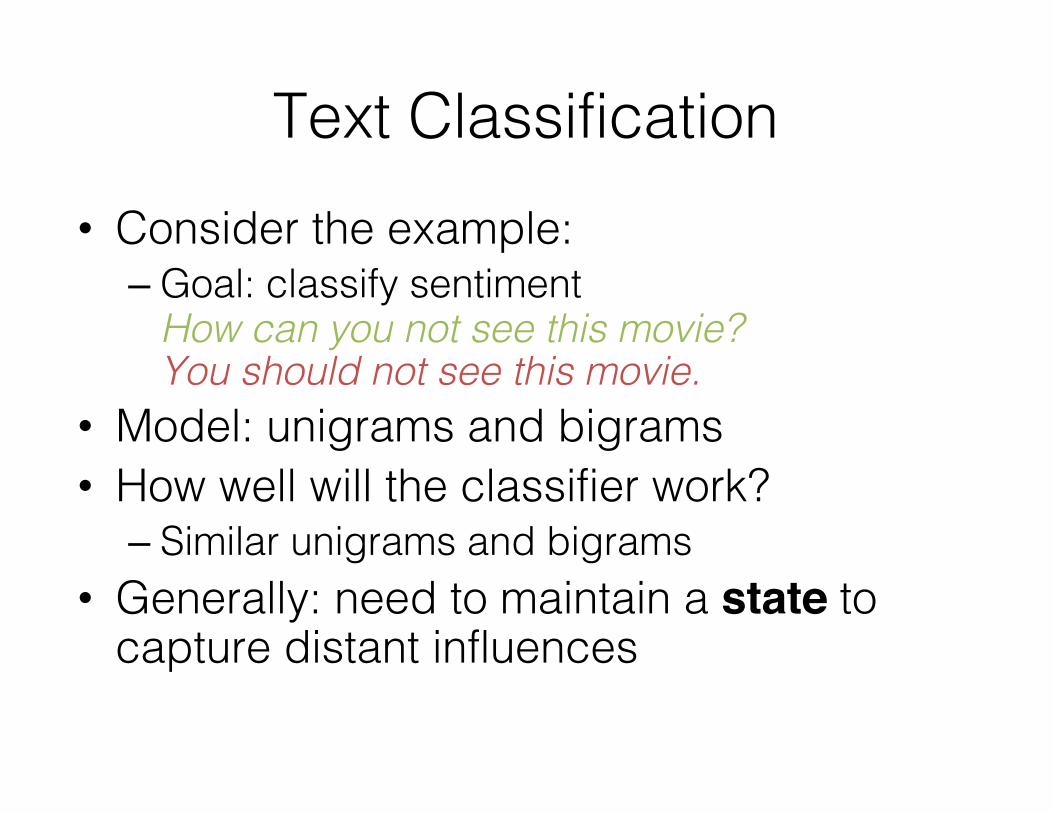
Text Classification• Consider the example:

– Goal: classify sentimentHow can you not see this movie?You should not see this movie.

• Model: unigrams and bigrams• How well will the classifier work?

– Similar unigrams and bigrams• Generally: need to maintain a state to

capture distant influences

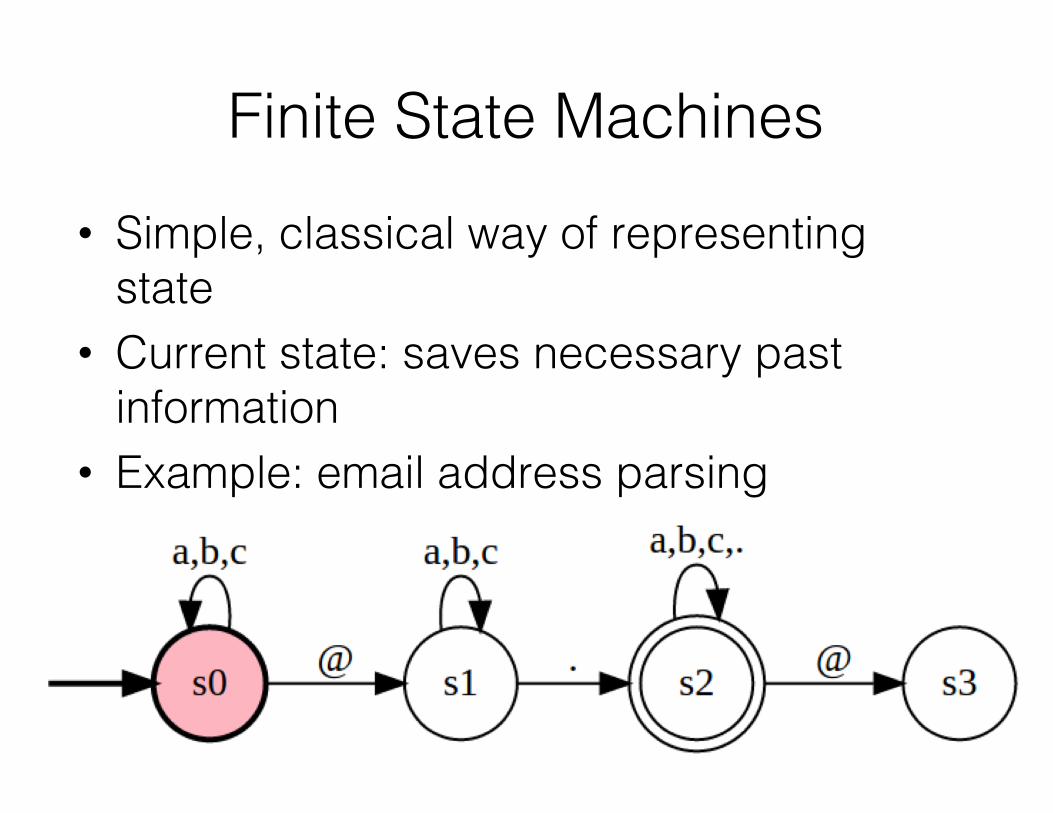
Finite State Machines• Simple, classical way of representing

state• Current state: saves necessary past

information• Example: email address parsing

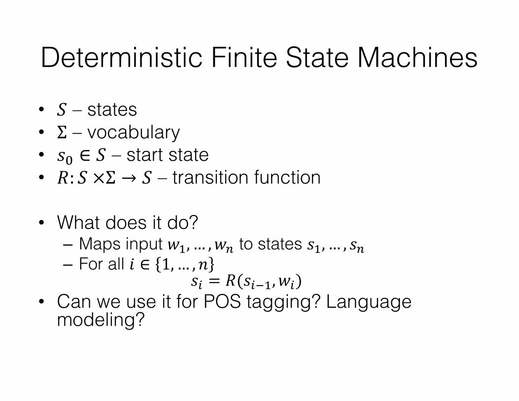
Deterministic Finite State Machines• 𝑆 – states• Σ – vocabulary • 𝑠$ ∈ 𝑆 – start state • 𝑅: 𝑆×Σ → 𝑆 – transition function

• What does it do?– Maps input 𝑤,,… ,𝑤/ to states 𝑠,, … , 𝑠/– For all 𝑖 ∈ 1,… , 𝑛

𝑠3 = 𝑅(𝑠36,, 𝑤3)• Can we use it for POS tagging? Language

modeling?

Types of State Machines• Acceptor

– Compute final state 𝑠/ and make a decision based on it: 𝑦 = 𝑂(𝑠/)

• Transducers– Apply function 𝑦3 = 𝑂(𝑠3) to produce output

for each intermediate state• Encoders

– Compute final state 𝑠/, and use it in another model

Recurrent Neural Networks• Motivation:

– Neural network model, but with state– How can we borrow ideas from FSMs?

• RNNs are FSMs …– … with a twist– No longer finite in the same sense

RNN

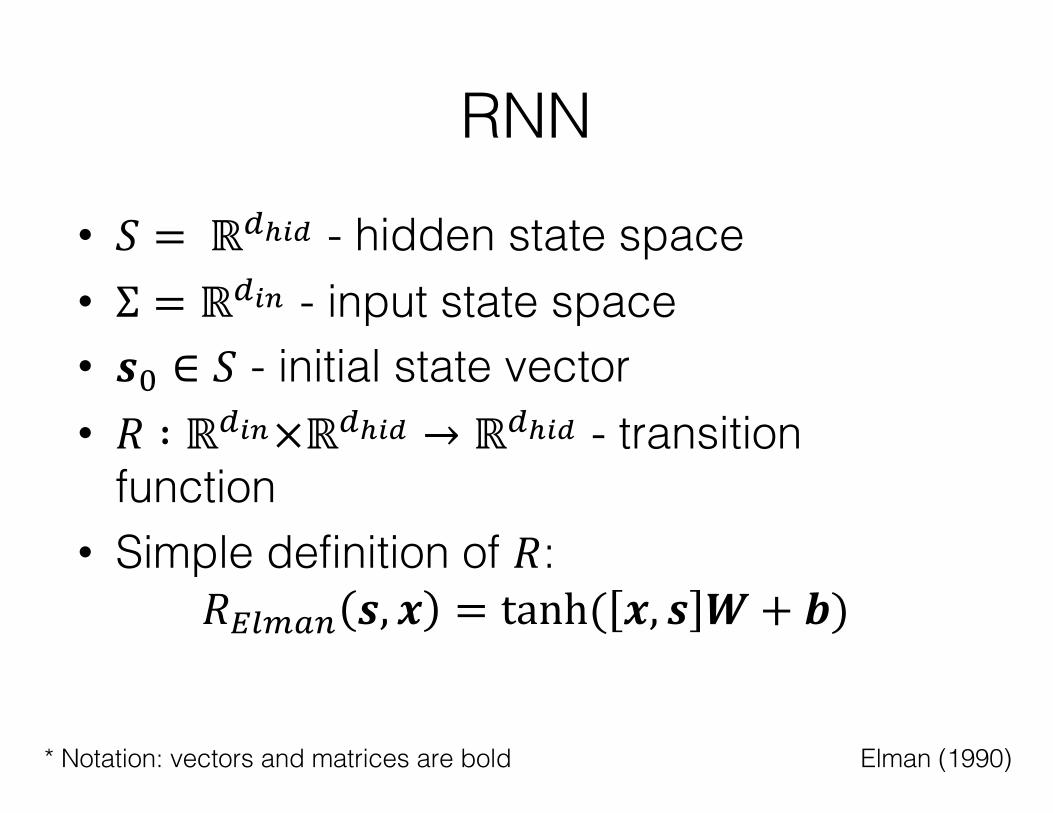
• 𝑆 = ℝ;<=> - hidden state space• Σ = ℝ;=? - input state space• 𝒔$ ∈ 𝑆 - initial state vector• 𝑅 ∶ ℝ;=?×ℝ;<=> → ℝ;<=> - transition

function• Simple definition of 𝑅:

𝑅BCDE/ 𝒔, 𝒙 = tanh( 𝒙, 𝒔 𝑾 + 𝒃)

Elman (1990)* Notation: vectors and matrices are bold

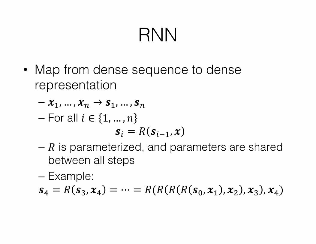
RNN• Map from dense sequence to dense

representation– 𝒙,, … , 𝒙/ → 𝒔,, … , 𝒔/– For all 𝑖 ∈ 1, … , 𝑛

𝒔3 = 𝑅 𝒔36,, 𝒙– 𝑅 is parameterized, and parameters are shared

between all steps– Example:𝒔N = 𝑅 𝒔O, 𝒙N = ⋯ = 𝑅(𝑅 𝑅 𝑅 𝒔$, 𝒙, , 𝒙Q , 𝒙O , 𝒙N)

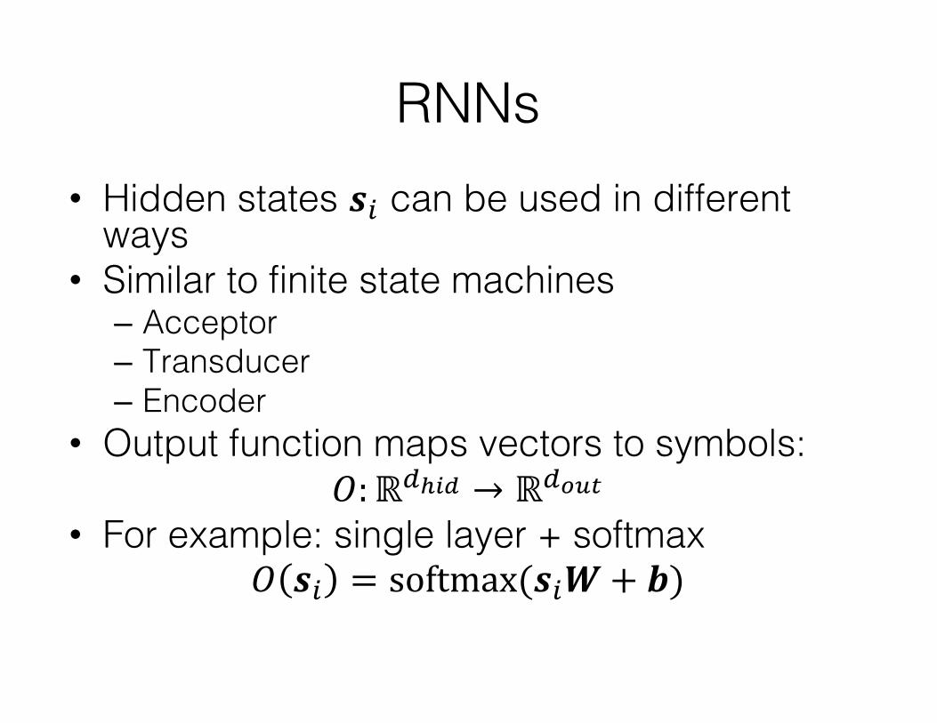
RNNs• Hidden states 𝒔3 can be used in different

ways• Similar to finite state machines

– Acceptor– Transducer– Encoder

• Output function maps vectors to symbols: 𝑂:ℝ;<=> → ℝ;RST

• For example: single layer + softmax𝑂 𝒔3 = softmax(𝒔3𝑾 + 𝒃)

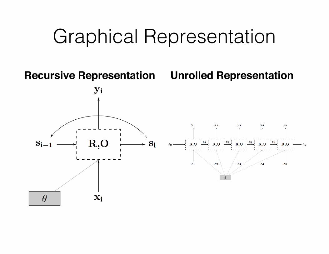
Graphical Representation

Recursive Representation Unrolled Representation

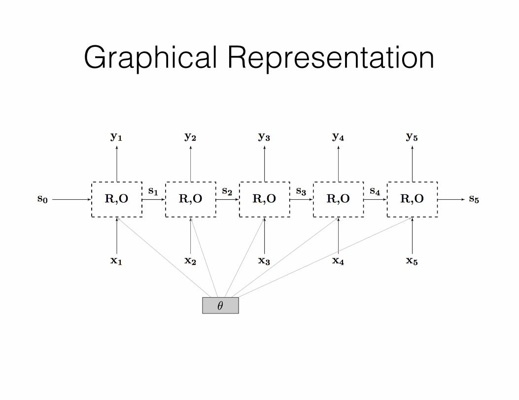
Graphical Representation

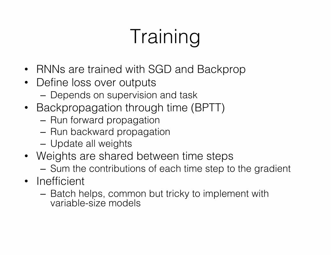
Training• RNNs are trained with SGD and Backprop• Define loss over outputs

– Depends on supervision and task• Backpropagation through time (BPTT)

– Run forward propagation– Run backward propagation– Update all weights

• Weights are shared between time steps– Sum the contributions of each time step to the gradient

• Inefficient– Batch helps, common but tricky to implement with

variable-size models

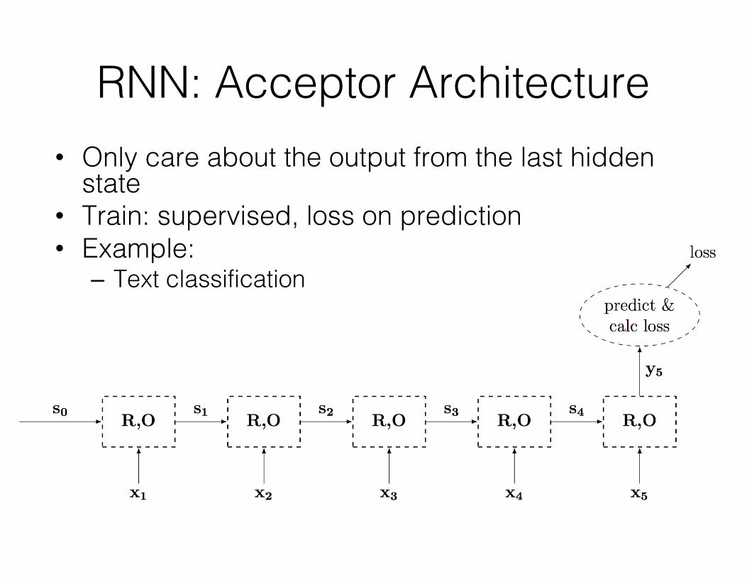
RNN: Acceptor Architecture• Only care about the output from the last hidden

state• Train: supervised, loss on prediction• Example:

– Text classification

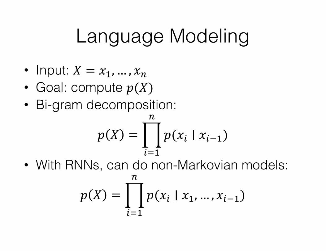
Language Modeling• Input: 𝑋 = 𝑥,,… , 𝑥/• Goal: compute 𝑝(𝑋)• Bi-gram decomposition:

𝑝 𝑋 =]𝑝(𝑥3 ∣ 𝑥36,)/

3_,• With RNNs, can do non-Markovian models:

𝑝 𝑋 =]𝑝(𝑥3 ∣ 𝑥,, … , 𝑥36,)/

3_,

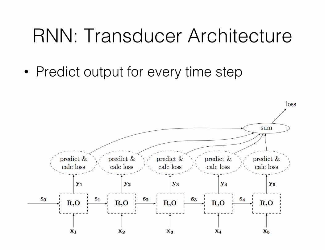
RNN: Transducer Architecture• Predict output for every time step

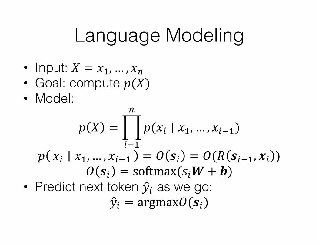
Language Modeling• Input: 𝑋 = 𝑥,,… , 𝑥/• Goal: compute 𝑝(𝑋)• Model:

𝑝 𝑋 =]𝑝(𝑥3 ∣ 𝑥,, … , 𝑥36,)/

3_,𝑝 𝑥3 𝑥,, … , 𝑥36, = 𝑂 𝒔3 = 𝑂(𝑅 𝒔36,, 𝒙3 )

𝑂 𝒔3 = softmax(𝑠3𝑾 + 𝒃)• Predict next token �̀�3 as we go:

�̀�3 = argmax𝑂(𝒔3)

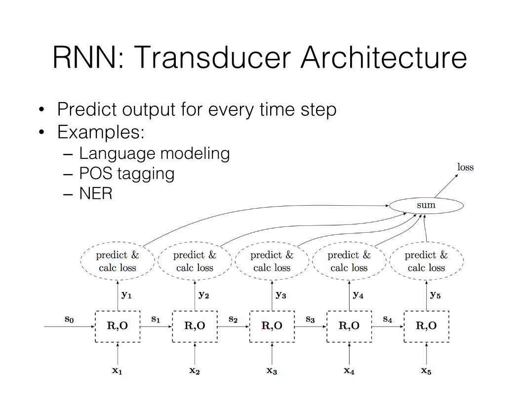
RNN: Transducer Architecture• Predict output for every time step• Examples:

– Language modeling– POS tagging– NER

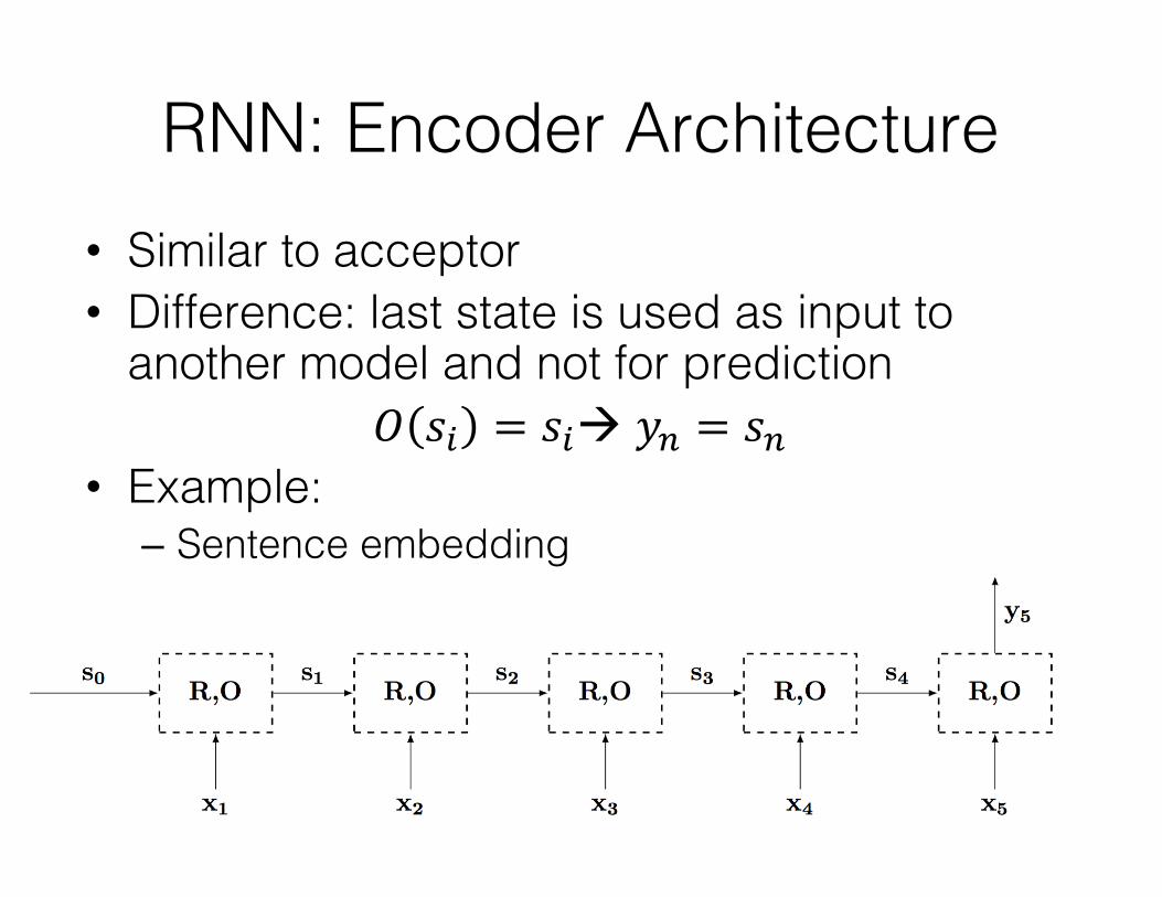
RNN: Encoder Architecture• Similar to acceptor• Difference: last state is used as input to

another model and not for prediction𝑂 𝑠3 = 𝑠3à 𝑦/ = 𝑠/

• Example:– Sentence embedding

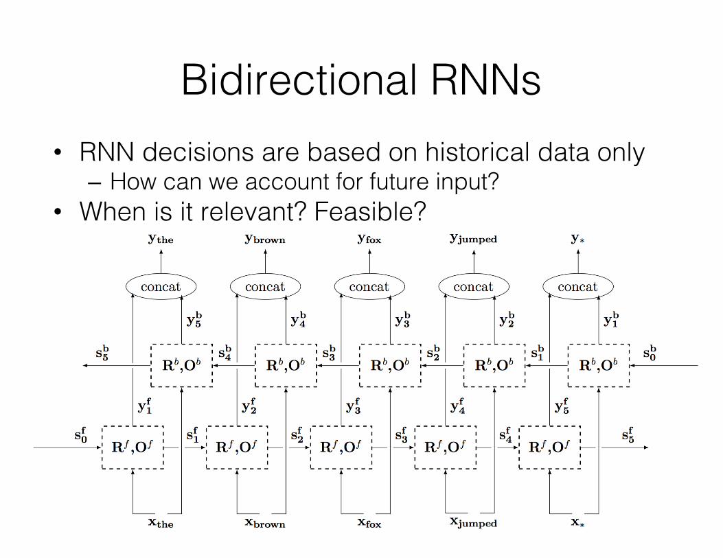
Bidirectional RNNs• RNN decisions are based on historical data only

– How can we account for future input?• When is it relevant? Feasible?

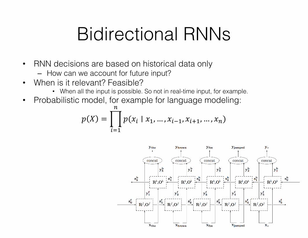
Bidirectional RNNs• RNN decisions are based on historical data only

– How can we account for future input?• When is it relevant? Feasible?

• When all the input is possible. So not in real-time input, for example.• Probabilistic model, for example for language modeling:

𝑝 𝑋 =]𝑝(𝑥3 ∣ 𝑥,, … , 𝑥36,, 𝑥3c,, … , 𝑥/)/

3_,

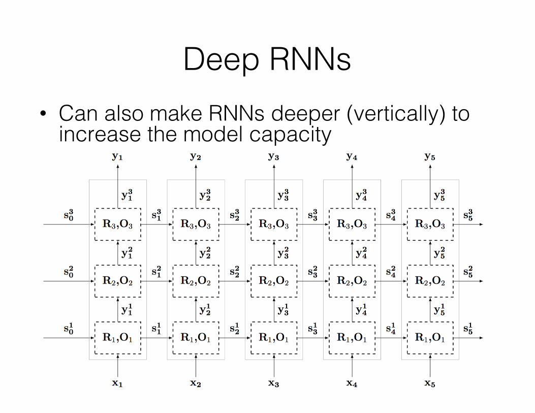
Deep RNNs• Can also make RNNs deeper (vertically) to

increase the model capacity

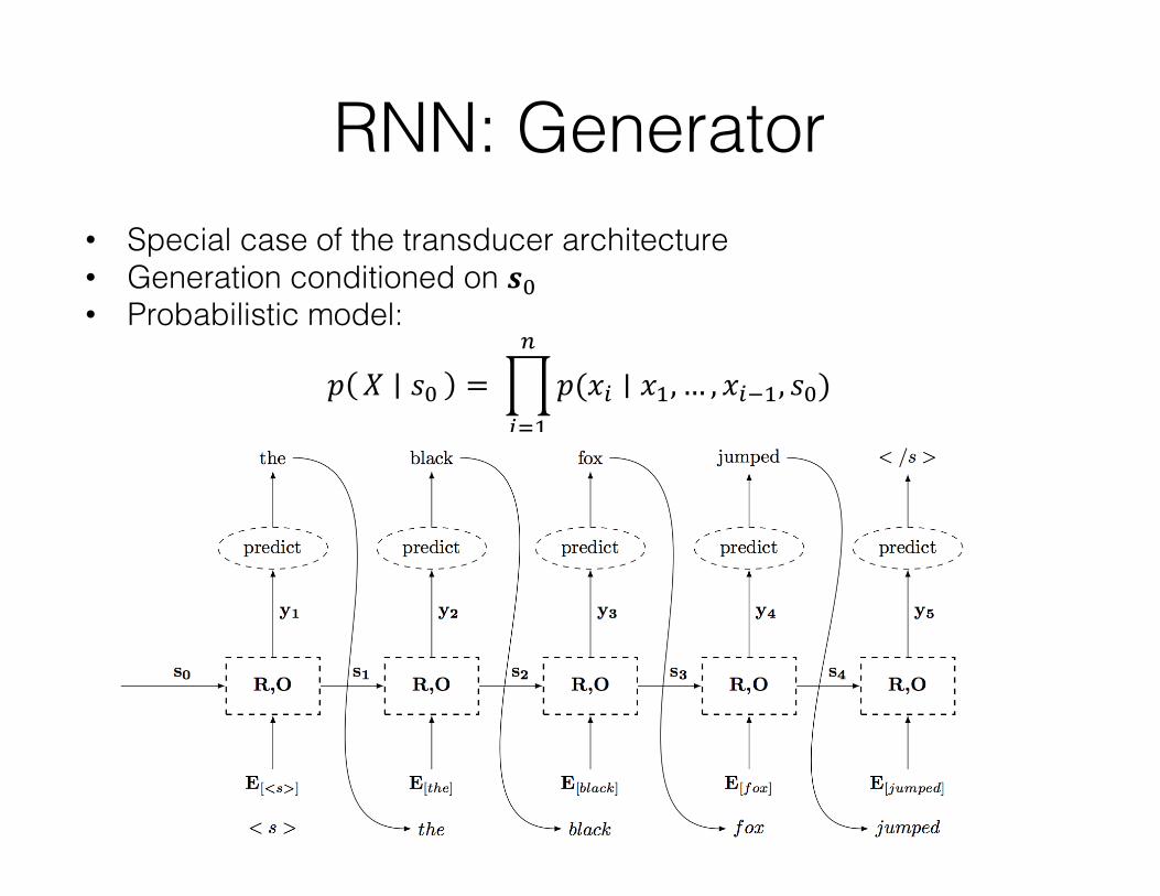
RNN: Generator• Special case of the transducer architecture• Generation conditioned on 𝒔$• Probabilistic model:

𝑝 𝑋 𝑠$ = ]𝑝(𝑥3 ∣ 𝑥,, … , 𝑥36,, 𝑠$)/

3_,

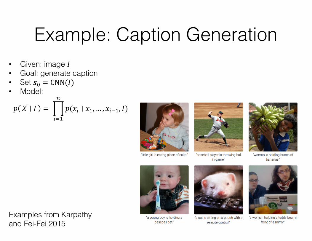
Example: Caption Generation• Given: image 𝐼• Goal: generate caption• Set 𝒔$ = CNN(𝐼)• Model:

𝑝 𝑋 𝐼 = ]𝑝(𝑥3 ∣ 𝑥,, … , 𝑥36,, 𝐼)/

3_,

Examples from Karpathyand Fei-Fei 2015

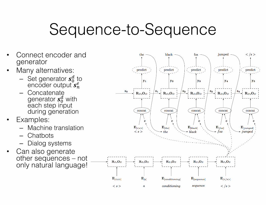
Sequence-to-Sequence• Connect encoder and

generator• Many alternatives:

– Set generator 𝒔$; to encoder output 𝒔/g

– Concatenate generator 𝒔$; with each step input during generation

• Examples:– Machine translation– Chatbots– Dialog systems

• Can also generate other sequences – not only natural language!

Long-range Interactions• Promise: Learn long-range interactions of

language from data• Example:

How can you not see this movie?You should not see this movie.

• Sometimes: requires ”remembering” early state– Key signal here is at 𝑠,, but gradient is at 𝑠/

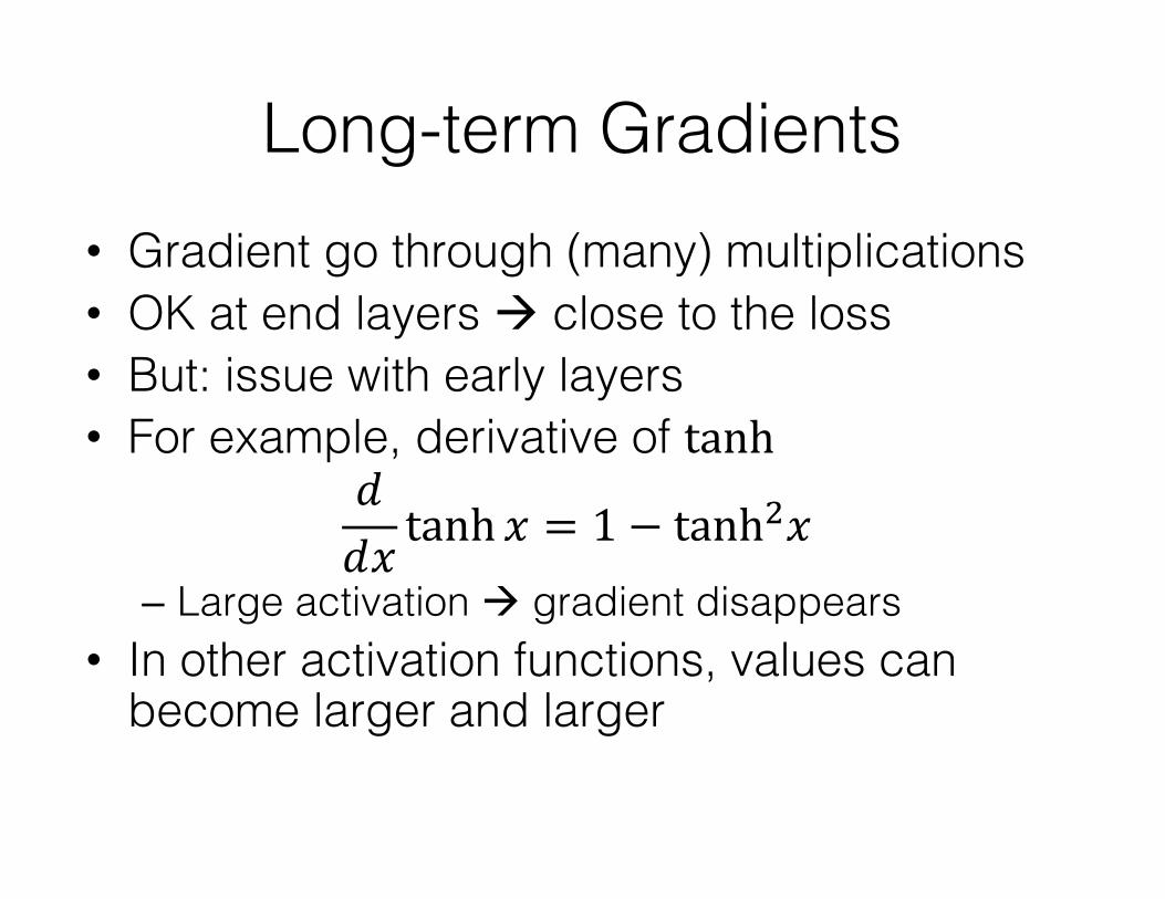
Long-term Gradients• Gradient go through (many) multiplications• OK at end layers à close to the loss• But: issue with early layers• For example, derivative of tanh

𝑑𝑑𝑥 tanh 𝑥 = 1 − tanhQ𝑥

– Large activation à gradient disappears• In other activation functions, values can

become larger and larger

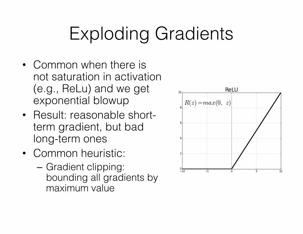
Exploding Gradients• Common when there is

not saturation in activation (e.g., ReLu) and we get exponential blowup

• Result: reasonable short-term gradient, but bad long-term ones

• Common heuristic:– Gradient clipping:

bounding all gradients by maximum value

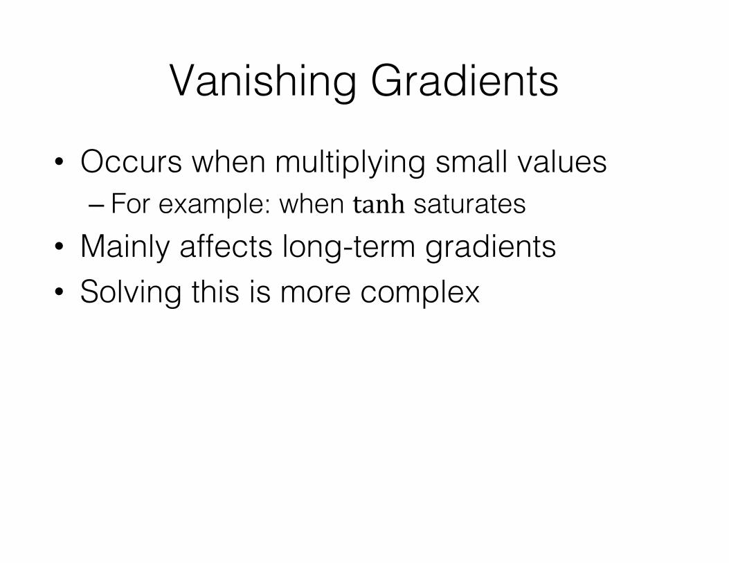
Vanishing Gradients• Occurs when multiplying small values

– For example: when tanh saturates• Mainly affects long-term gradients• Solving this is more complex

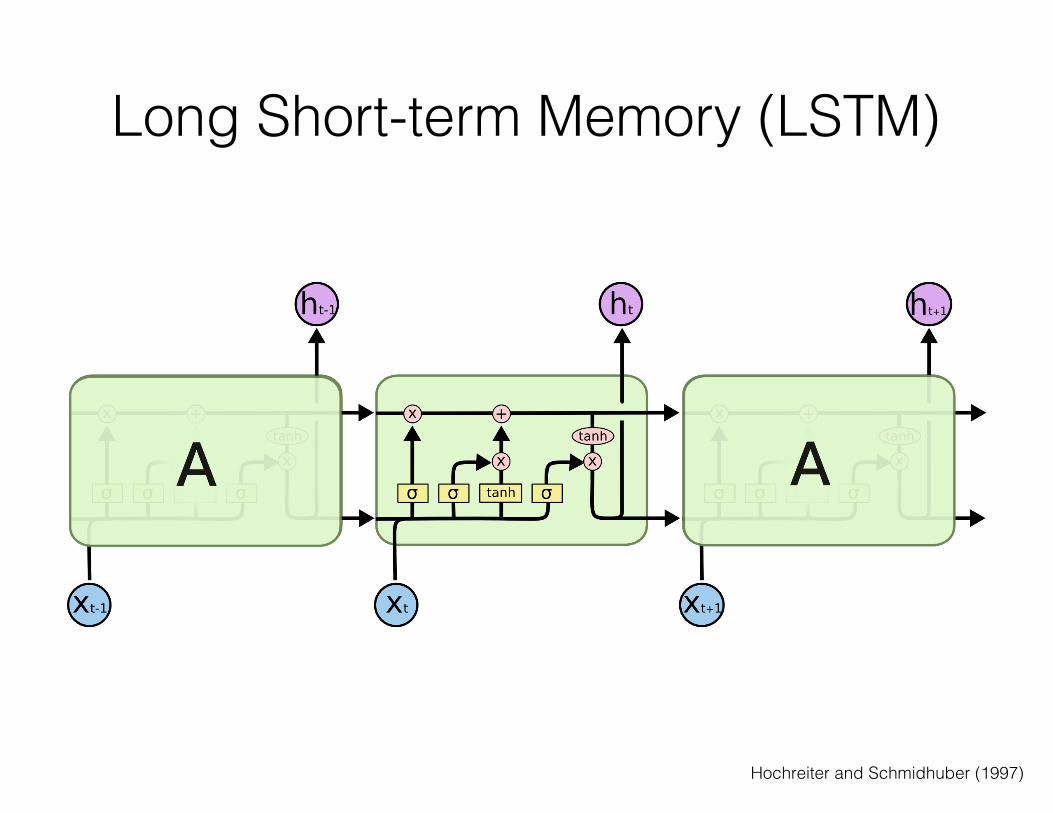
Long Short-term Memory (LSTM)

Hochreiter and Schmidhuber (1997)

LSTM vs. Elman RNN

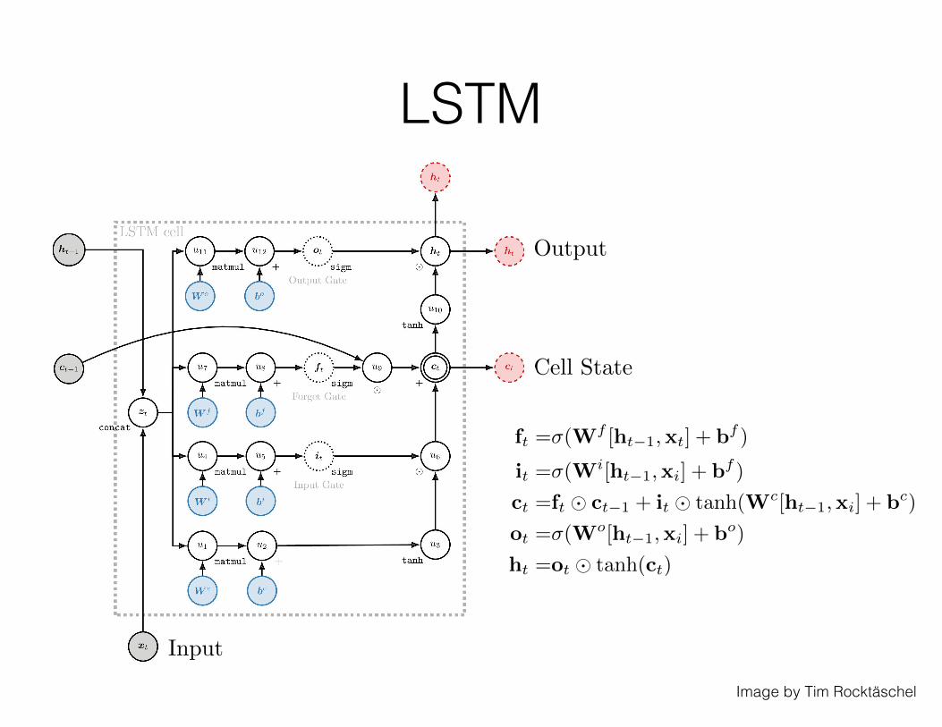
LSTM

Image by Tim Rocktäschel

f

t

=�(Wf [ht�1,xt

] + b

f )

i

t

=�(Wi[ht�1,xi

] + b

f )

c

t

=f

t

� c

t�1 + i

t

� tanh(Wc[ht�1,xi

] + b

c)

o

t

=�(Wo[ht�1,xi

] + b

o)

h

t

=o

t

� tanh(ct

)

Cell State

Output

Input