CS498-EACS498-EAReasoning in AIReasoning in AILecture #10Lecture #10

Instructor: Eyal AmirInstructor: Eyal Amir

Fall Semester 2009Fall Semester 2009

Some slides in this set were adopted from Eran Segal

Known Structure, Complete Data• Goal: Parameter estimation• Data does not contain missing values

P(Y|X1,X2)

X1 X2 y0 y1

x10 x2

0 1 0

x10 x2

1 0.2 0.8

x11 x2

0 0.1 0.9

x11 x2

1 0.02 0.98

X1

Y

X2

InducerInducerInducerInducer

X1 X2 Y

x10 x2

1 y0

x11 x2

0 y0

x10 x2

1 y1

x10 x2

0 y0

x11 x2

1 y1

x10 x2

1 y1

x11 x2

0 y0

InputData

X1

Y

X2Initial

network

Maximum Likelihood Estimator• General case

– Observations: MH heads and MT tails

– Find maximizing likelihood– Equivalent to maximizing log-likelihood

– Differentiating the log-likelihood and solving for we get that the maximum likelihood parameter is:

TH MMTH MML )1():,(

)1log(log):,( THTH MMMMl

TH

H

MM

M

Sufficient Statistics for Multinomial• A sufficient statistics for a dataset D over a variable Y

with k values is the tuple of counts <M1,...Mk> such that Mi is the number of times that the Y=yi in D

• Sufficient statistic– Define s(x[i]) as a tuple of dimension k– s(x[i])=(0,...0,1,0,...,0)

–

(1,...,i-1) (i+1,...,k)

k

i

Dsi

iDL1

)():(

Properties of ML Estimator

• Unbiased– M number of

occurences of H– N total no.experiments = Pr(H)

• Variance

N

ii

N

ii

XN

HeadXNN

ME

1

1

...1

)Pr(1

)(

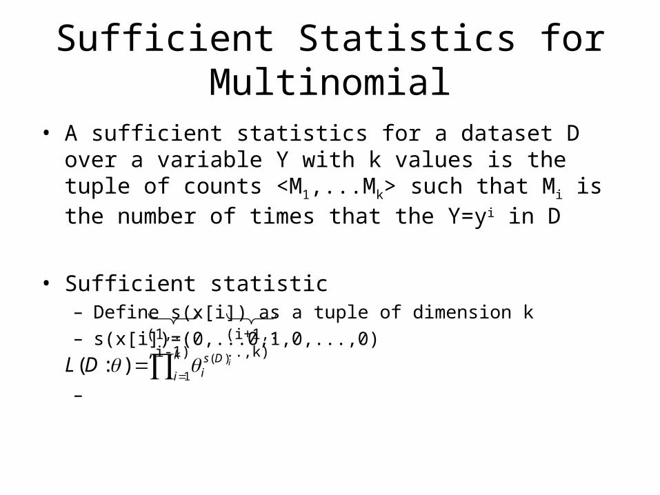
Sufficient Statistic for Gaussian

• Gaussian distribution:

• Rewrite as

sufficient statistics for Gaussian: s(x[i])=<1,x,x2>

2

2

12

2

1)(),(~)(

x

eXpNXP if

2

2

222

2

1exp

2

1)(

xxXp

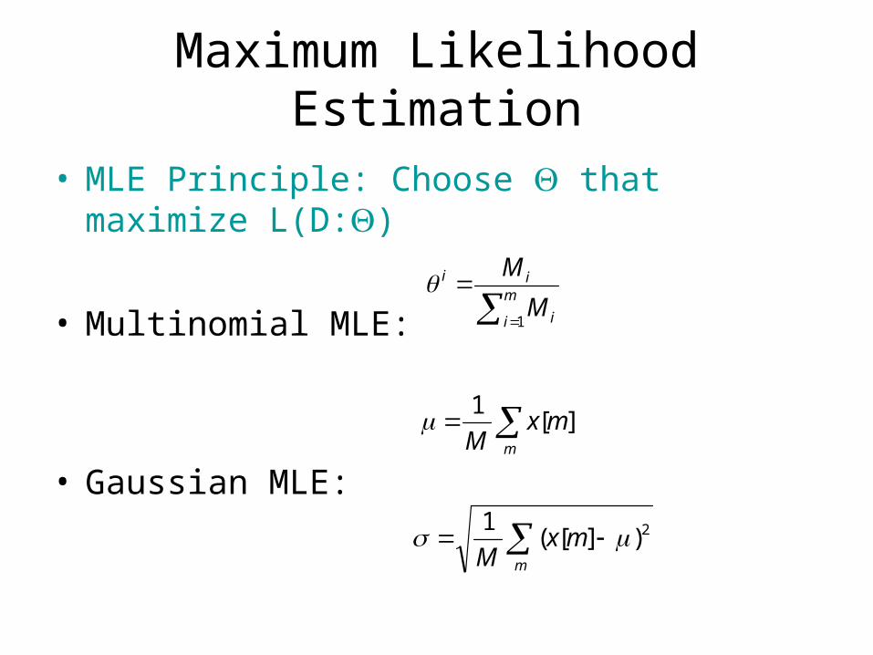
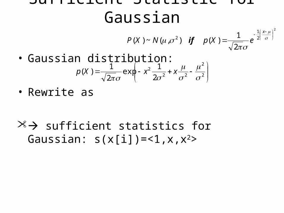
Maximum Likelihood Estimation• MLE Principle: Choose that maximize L(D:)

• Multinomial MLE:

• Gaussian MLE: m

mxM

][1

m

i i

ii

M

M

1

m

mxM

2)][(1

MLE for Bayesian Networks• Parameters

x0, x1

y0|x0, y1|x0, y0|x1, y1|x1

• Data instance tuple: <x[m],y[m]>• Likelihood

X

Y

Y

X y0 y1

x0 0.95

0.05

x1 0.2 0.8

X

x0 x1

0.7 0.3

):][|][():][(

):][|][():][(

):][],[():(

11

1

1

M

m

M

m

M

m

M

m

mxmyPmxP

mxmyPmxP

mymxPDL

Likelihood decomposes into two separate terms, one for each variable

MLE for Bayesian Networks• Terms further decompose by CPDs:

• By sufficient statistics

where M[x0,y0] is the number of data instances in which X takes the value x0 and Y takes the value y0

• MLE

0 1

10

0 1

][: ][:||

][: ][:||

1

):][|][():][|][(

):][|][():][|][():][|][(

xmxm xmxmxYxY

xmxm xmxmXYXY

M

m

mxmyPmxmyP

mxmyPmxmyPmxmyP

1

11

1

01

11

][:

],[

|

],[

||):][|][(

xmxm

yxM

xY

yxM

xYxYmxmyP

][

],[

],[],[

],[1

01

1101

01

| 10

xM

yxM

yxMyxM

yxMxy

MLE for Bayesian Networks• Likelihood for Bayesian network

if Xi|Pa(Xi) are disjoint then MLE can be computed by

maximizing each local likelihood separately

ii

i miii

m iiii

m

DL

mPamxP

mPamxP

mxPDL

):(

):][|][(

):][|][(

):][():(

MLE for Table CPD BayesNets• Multinomial CPD

• For each value xX we get an independent multinomial problem where the MLE is

)( )(

],[|

][|][| ):(

Xx

xx

XX

Val YValy

yMy

mmmyYY DL

][

],[| x

xx M

yM i

y i

MLE for Tree CPDs• Assume tree CPD with known tree structure

y0 y1

z1z0

Z

Y

x0|y0,x1|y0

x0|y1,z1,x1|y1,z1x0|y1,z1,x1|y1,z1

Y

X

Z

],,[

,|

],,[

,|

],[

|

],,[

,|

],,[

,|

],,[],,[

|

],,[

,|

],,[

,|

],,[

|

],,[

|

],,[,|

11

11

01

01

0

0

11

11

01

01

1000

0

11

11

01

01

10

0

00

0

),,|(

xzyM

zyx

xzyM

zyx

xyM

yx

xzyM

zyx

xzyM

zyx

xzyMxzyM

yx

xzyM

zyx

xzyM

zyx

xzyM

yx

xzyM

yx

y z x

xzyMZYXzyxP

):( ,| ZYXDL

Terms for <y0,z0> and <y0,z1> can be combined

Optimization can be done by leaves

MLE for Tree CPD BayesNets• Tree CPD T, leaves l

• For each value lLeaves(T) we get an independent multinomial problem where the MLE is

)( )(

],[|

])[(|][

|| ):][|][():(

TLeavesl YValy

ycMly

mmlmy

mYYY

l

mmyPDL

x

XX x

][

],[|

l

il

ly cM

ycMi

ll

il yMcM

)(:

],[][xx

x

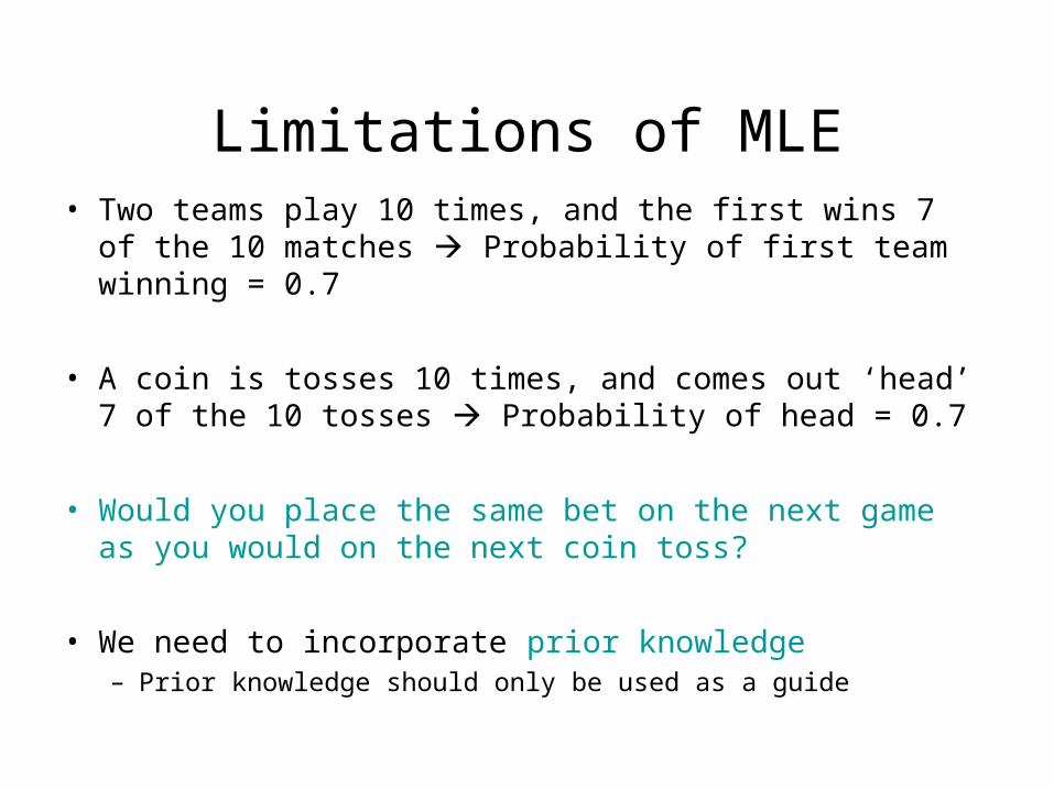
Limitations of MLE• Two teams play 10 times, and the first wins 7 of the 10

matches Probability of first team winning = 0.7

• A coin is tosses 10 times, and comes out ‘head’ 7 of the 10 tosses Probability of head = 0.7

• Would you place the same bet on the next game as you would on the next coin toss?

• We need to incorporate prior knowledge – Prior knowledge should only be used as a guide

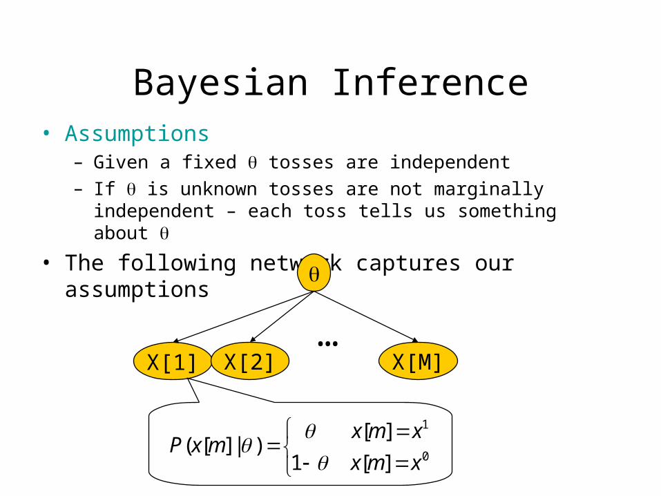
Bayesian Inference• Assumptions

– Given a fixed tosses are independent– If is unknown tosses are not marginally independent – each

toss tells us something about

• The following network captures our assumptions

X[1] X[M]X[2]…

0

1

][1

][)|][(

xmx

xmxmxP

Bayesian Inference• Joint probabilistic model

• Posterior probability over

TH MM

M

i

P

ixPP

PMxxPMxxP

)1()(

)|][()(

)()|][],...,1[()],[],...,1[(

1

X[1] X[M]X[2] …

])[],...,1[(

)()|][],...,1[(])[],...,1[|(

MxxP

PMxxPMxxP

Likelihood

Prior

Normalizing factor

For a uniform prior, posterior is the

normalized likelihood

Bayesian Prediction• Predict the data instance from the previous ones

• Solve for uniform prior P()=1 and binomial variable

dMxxPMxP

dMxxPMxxMxP

dMxxMxP

MxxMxP

])[],...,1[|()|]1[(

])[],...,1[|()],[],...,1[|]1[(

])[],...,1[|],1[(

])[],...,1[|]1[(

2

1

)1(])[],...,1[(

1)],[],...,1[|]1[( 1

TH

H

MM

MM

MMxxP

MxxxMxP TH

Example: Binomial Data

• Prior: uniform for in [0,1]– P() = 1

P( |D) is proportional to the likelihood L(D:)

• MLE for P(X=H) is 4/5 = 0.8

• Bayesian prediction is 5/7

)|][],1[(])[],1[|( MxxPMxxP

7142.07

5)|()|]1[( dDPDHMxP

0 0.2 0.4 0.6 0.8 1

(MH,MT ) = (4,1)

Dirichlet Priors• A Dirichlet prior is specified by a set of (non-

negative) hyperparameters 1,...k so that

~ Dirichlet(1,...k) if

– where and

– Intuitively, hyperparameters correspond to the number of imaginary examples we saw before starting the experiment

k

kk

ZP 11

)( )(

)(

1

1

k

i i

k

i iZ

0

1)( dtetx tx

Dirichlet Priors – Example

0

0.5

1

1.5

2

2.5

3

3.5

4

4.5

5

0 0.2 0.4 0.6 0.8 1

Dirichlet(1,1)Dirichlet(2,2)

Dirichlet(0.5,0.5)Dirichlet(5,5)

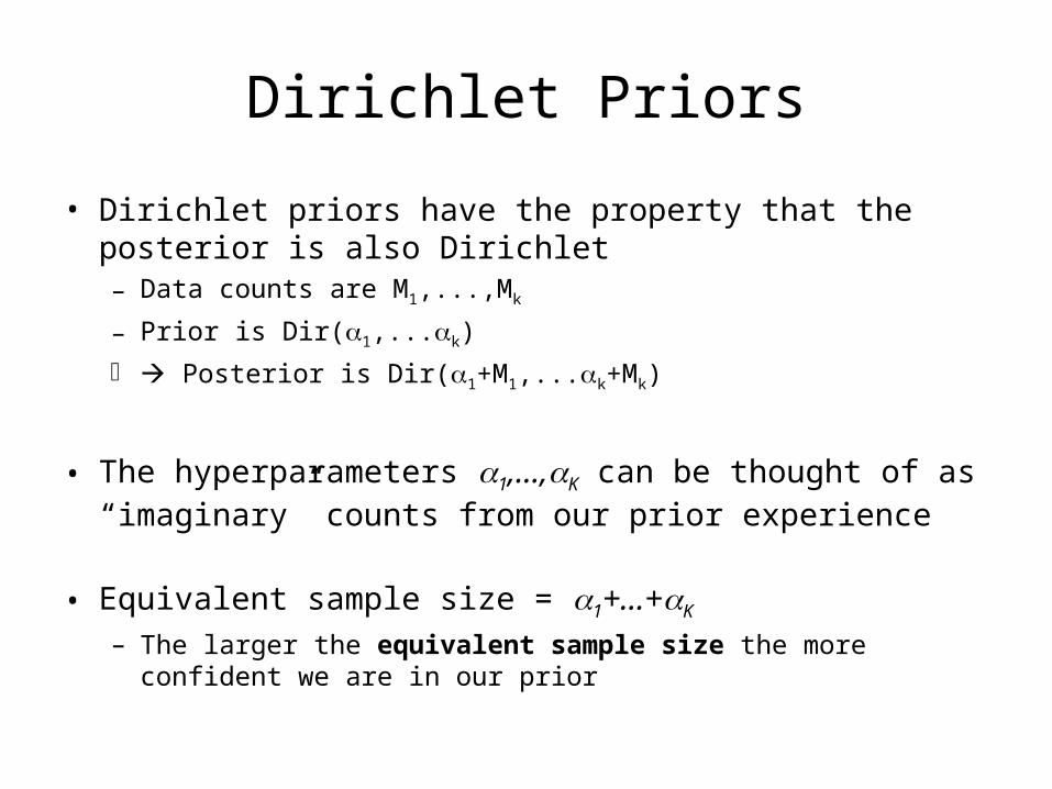
Dirichlet Priors

• Dirichlet priors have the property that the posterior is also Dirichlet– Data counts are M1,...,Mk

– Prior is Dir(1,...k)

Posterior is Dir(1+M1,...k+Mk)

• The hyperparameters 1,…,K can be thought of as “imaginary” counts from our prior experience

• Equivalent sample size = 1+…+K – The larger the equivalent sample size the more confident we are

in our prior

Effect of Priors

0.15

0.2

0.25

0.3

0.35

0.4

0.45

0.5

0.55

0 20 40 60 80 1000

0.1

0.2

0.3

0.4

0.5

0.6

0 20 40 60 80 100

Different strength H + T Fixed ratio H / T

Fixed strength H + T

Different ratio H / T

• Prediction of P(X=H) after seeing data with MH=1/4MT as a function of the sample size

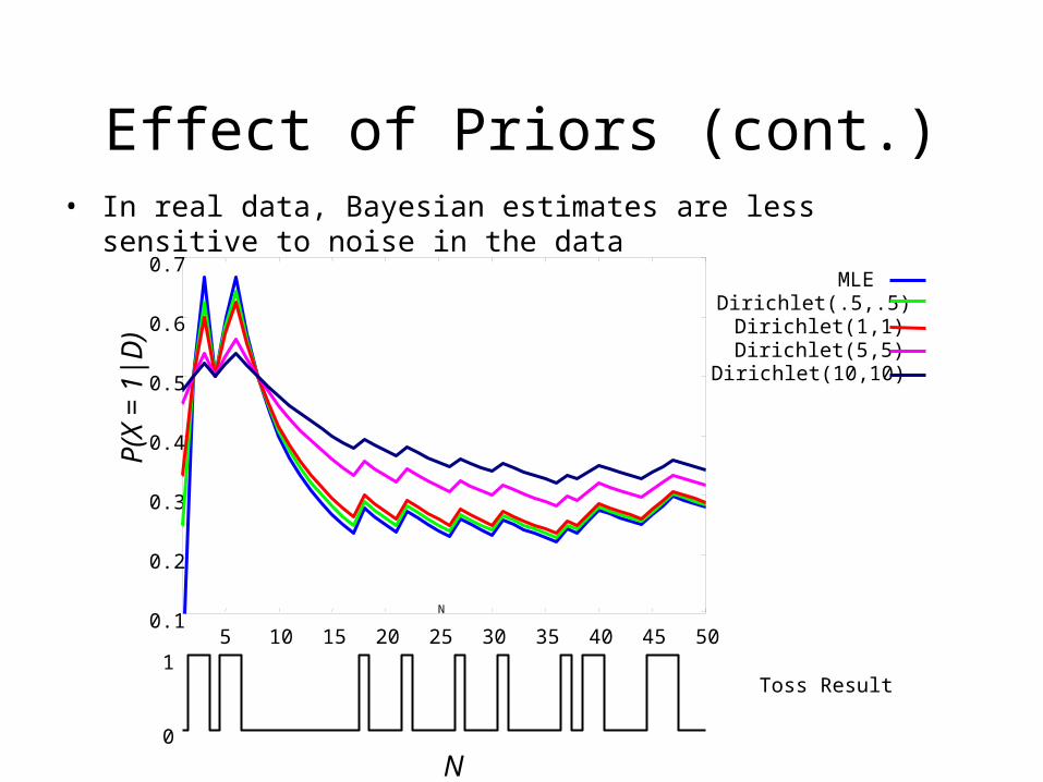
Effect of Priors (cont.)

0.1

0.2

0.3

0.4

0.5

0.6

0.7

5 10 15 20 25 30 35 40 45 50

P(X

= 1

|D)

N

MLEDirichlet(.5,.5)

Dirichlet(1,1)Dirichlet(5,5)

Dirichlet(10,10)

N

0

1Toss Result

• In real data, Bayesian estimates are less sensitive to noise in the data

General Formulation• Joint distribution over D,

• Posterior distribution over parameters

• P(D) is the marginal likelihood of the data

• As we saw, likelihood can be described compactly using sufficient statistics

• We want conditions in which posterior is also compact

)()|(),( PDPDP

)(

)()|()|(

DP

PDPDP

dPDPDP )()|()(

Conjugate Families• A family of priors P(:) is conjugate to a model P(|) if for any

possible dataset D of i.i.d samples from P(|) and choice of hyperparameters for the prior over , there are hyperparameters ’ that describe the posterior, i.e.,P(:’) P(D|)P(:)– Posterior has the same parametric form as the prior

– Dirichlet prior is a conjugate family for the multinomial likelihood

• Conjugate families are useful since:– Many distributions can be represented with hyperparameters

– They allow for sequential update within the same representation

– In many cases we have closed-form solutions for prediction

Bayesian Estimation in BayesNets

• Instances are independent given the parameters– (x[m’],y[m’]) are d-separated from (x[m],y[m]) given

• Priors for individual variables are a priori independent– Global independence of parameters

X

X[1] X[M]X[2] …X

Y

Bayesian network

Bayesian network for parameter estimation

Y[1] Y[M]Y[2] …

Y|X

i

XPaX iiPP )()( )(|

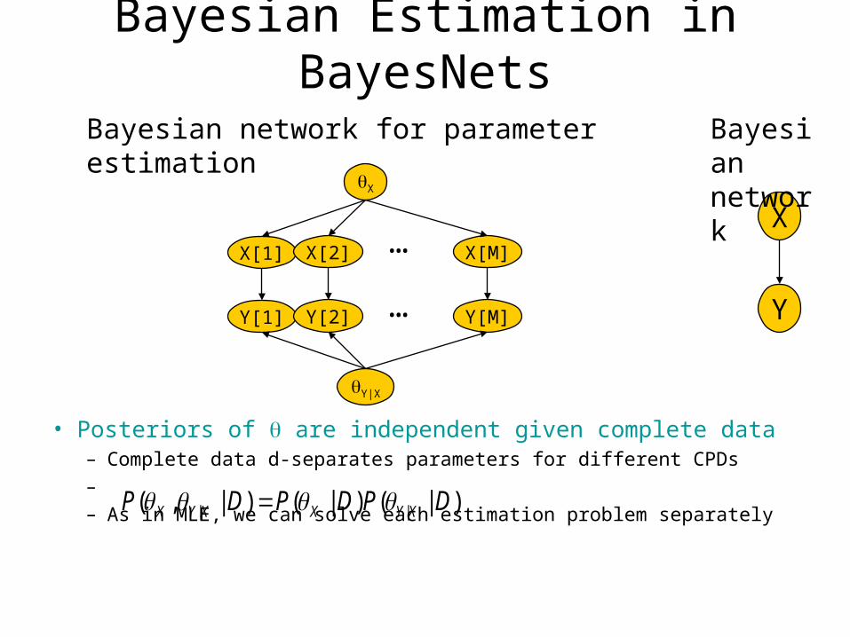
Bayesian Estimation in BayesNets

• Posteriors of are independent given complete data– Complete data d-separates parameters for different CPDs– – As in MLE, we can solve each estimation problem separately

X

X[1] X[M]X[2] …X

Y

Bayesian network

Bayesian network for parameter estimation

Y[1] Y[M]Y[2] …

Y|X

)|()|()|,( || DPDPDP XYXXYX

Bayesian Estimation in BayesNets

• Posteriors of are independent given complete data– Also holds for parameters within families

– Note context specific independence between Y|X=0 and Y|

X=1 when given both X and Y

X

X[1] X[M]X[2] …X

Y

Bayesian network

Bayesian network for parameter estimation

Y[1] Y[M]Y[2] …

Y|X=0 Y|X=1

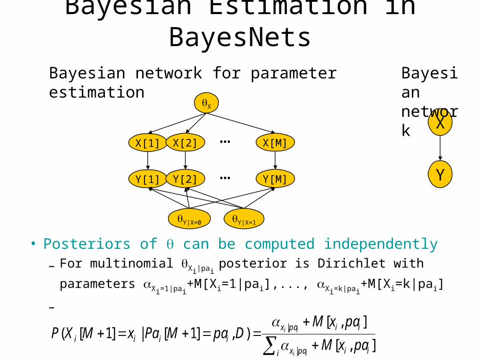
Bayesian Estimation in BayesNets

• Posteriors of can be computed independently

– For multinomial Xi|pai posterior is Dirichlet with parameters Xi=1|

pai+M[Xi=1|pai],..., Xi=k|pai

+M[Xi=k|pai]

–

X

X[1] X[M]X[2] …X

Y

Bayesian network

Bayesian network for parameter estimation

Y[1] Y[M]Y[2] …

Y|X=0 Y|X=1

i iipax

iipaxiiii paxM

paxMDpaMPaxMXP

ii

ii

],[

],[),]1[|]1[(

|

|

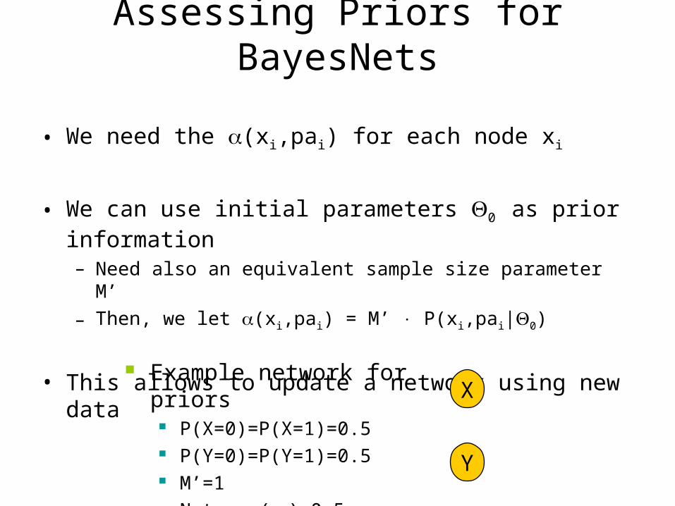
Assessing Priors for BayesNets

• We need the (xi,pai) for each node xi

• We can use initial parameters 0 as prior information– Need also an equivalent sample size parameter M’

– Then, we let (xi,pai) = M’ P(xi,pai|0)

• This allows to update a network using new data

X

Y

Example network for priors P(X=0)=P(X=1)=0.5 P(Y=0)=P(Y=1)=0.5 M’=1 Note: (x0)=0.5

(x0,y0)=0.25

Case Study: ICU Alarm Network

• The “Alarm” network– 37 variables

• Experiment– Sample instances– Learn parameters

• MLE• Bayesian

PCWP CO

HRBP

HREKG HRSAT

ERRCAUTERHRHISTORY

CATECHOL

SAO2 EXPCO2

ARTCO2

VENTALV

VENTLUNG VENITUBE

DISCONNECT

MINVOLSET

VENTMACHKINKEDTUBEINTUBATIONPULMEMBOLUS

PAP SHUNT

ANAPHYLAXIS

MINOVL

PVSAT

FIO2

PRESS

INSUFFANESTHTPR

LVFAILURE

ERRBLOWOUTPUTSTROEVOLUMELVEDVOLUME

HYPOVOLEMIA

CVP

BP

Case Study: ICU Alarm Network

0

0.2

0.4

0.6

0.8

1

1.2

1.4

0 500 1000 1500 2000 2500 3000 3500 4000 4500 5000

KL

Div

erg

en

ce

M

MLEBayes w/ Uniform Prior, M'=5

Bayes w/ Uniform Prior, M'=10Bayes w/ Uniform Prior, M'=20Bayes w/ Uniform Prior, M'=50

• MLE performs worst• Prior M’=5 provides best smoothing

Parameter Estimation Summary

• Estimation relies on sufficient statistics– For multinomials these are of the form M[xi,pai]

– Parameter estimation

• Bayesian methods also require choice of priors• MLE and Bayesian are asymptotically equivalent• Both can be implemented in an online manner by

accumulating sufficient statistics

][

],[),|( ,

ipa

iipaxii paM

paxMDpaxP

i

ii

][

],[ˆ|

i

iipax paM

paxMii

MLE Bayesian (Dirichlet)

THE END

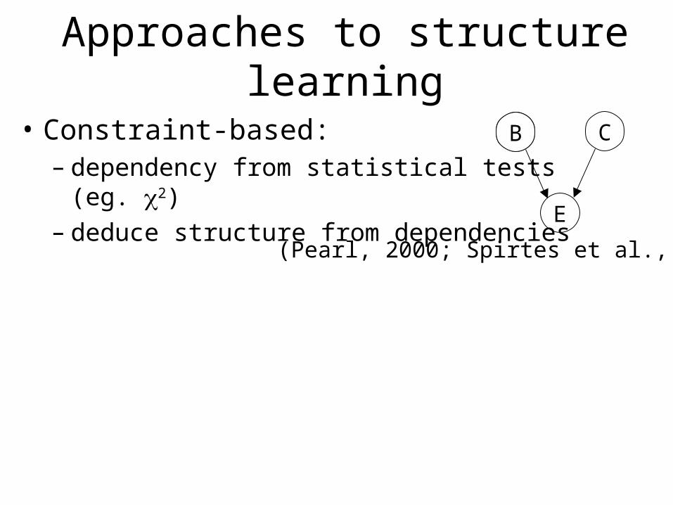
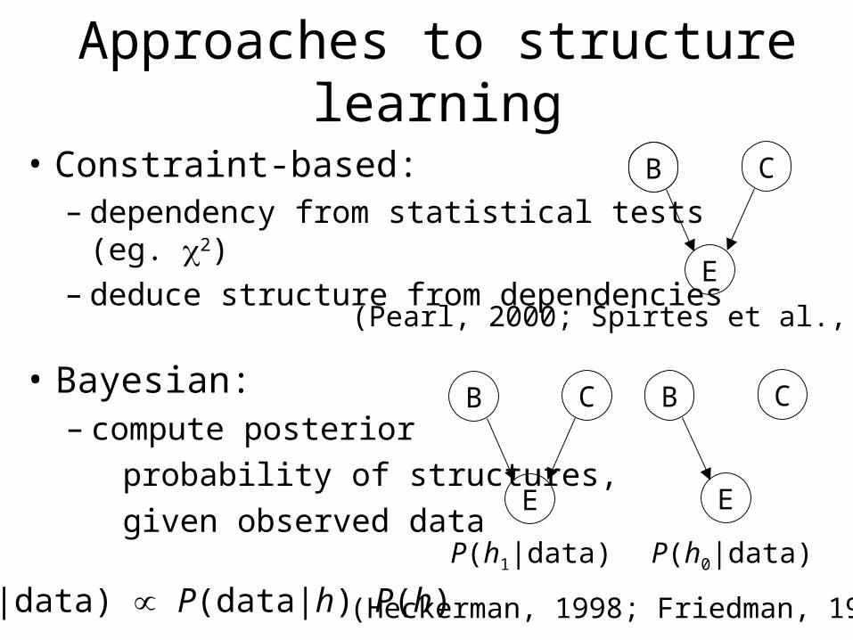
Approaches to structure learning

• Constraint-based:– dependency from statistical tests (eg. 2)– deduce structure from dependencies E

B CB

(Pearl, 2000; Spirtes et al., 1993)

Approaches to structure learning

E

B CB• Constraint-based:– dependency from statistical tests (eg. 2)– deduce structure from dependencies

(Pearl, 2000; Spirtes et al., 1993)

Approaches to structure learning

E

B CB• Constraint-based:– dependency from statistical tests (eg. 2)– deduce structure from dependencies

(Pearl, 2000; Spirtes et al., 1993)

Approaches to structure learning

E

B CB

Attempts to reduce inductive problem to deductive problem

• Constraint-based:– dependency from statistical tests (eg. 2)– deduce structure from dependencies

(Pearl, 2000; Spirtes et al., 1993)

Approaches to structure learning

E

B CB

• Bayesian:– compute posterior

probability of structures,

given observed dataE

B C

E

B C

P(h|data) P(data|h) P(h)

P(h1|data) P(h0|data)

• Constraint-based:– dependency from statistical tests (eg. 2)– deduce structure from dependencies

(Pearl, 2000; Spirtes et al., 1993)

(Heckerman, 1998; Friedman, 1999)

Bayesian Occam’s Razor

All possible data sets d

P(d

| h

)

h0 (no relationship)

h1 (relationship)

P(d

d | h) 1For any model h,

Unknown Structure, Complete Data• Goal: Structure learning & parameter estimation• Data does not contain missing values

P(Y|X1,X2)

X1 X2 y0 y1

x10 x2

0 1 0

x10 x2

1 0.2 0.8

x11 x2

0 0.1 0.9

x11 x2

1 0.02 0.98

X1

Y

X2

InducerInducerInducerInducer

X1 X2 Y

x10 x2

1 y0

x11 x2

0 y0

x10 x2

1 y1

x10 x2

0 y0

x11 x2

1 y1

x10 x2

1 y1

x11 x2

0 y0

InputData

X1

Y

X2Initial

network

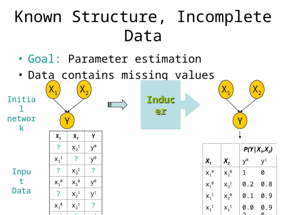
Known Structure, Incomplete Data• Goal: Parameter estimation• Data contains missing values

P(Y|X1,X2)

X1 X2 y0 y1

x10 x2

0 1 0

x10 x2

1 0.2 0.8

x11 x2

0 0.1 0.9

x11 x2

1 0.02 0.98

X1

Y

X2

InducerInducerInducerInducer

X1 X2 Y

? x21 y0

x11 ? y0

? x21 ?

x10 x2

0 y0

? x21 y1

x10 x2

1 ?

x11 ? y0

InputData

Initial network

X1

Y

X2

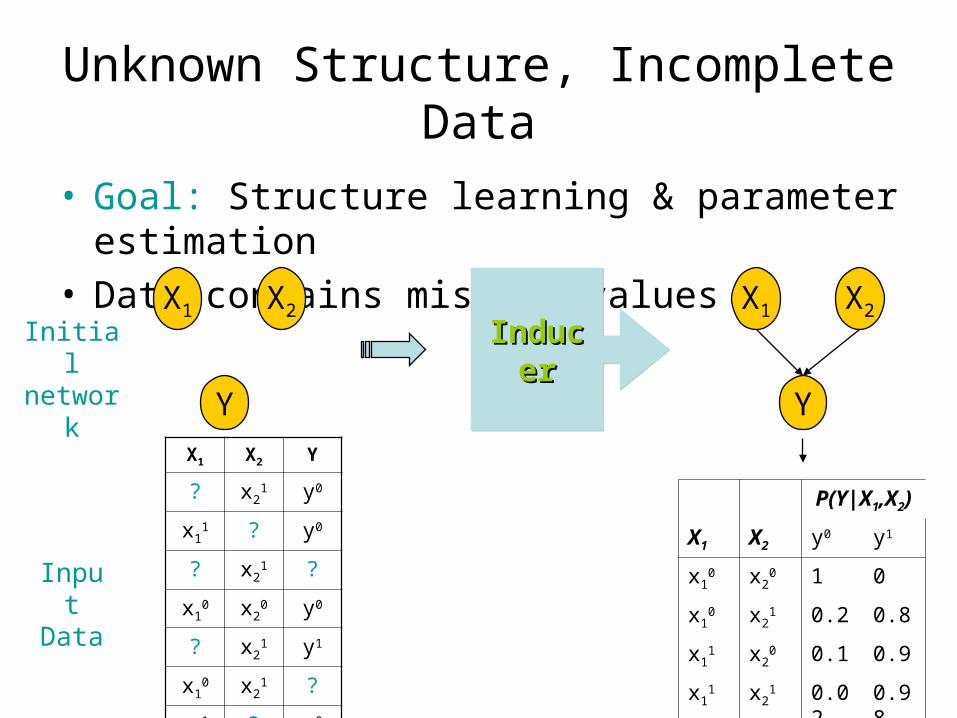
Unknown Structure, Incomplete Data

• Goal: Structure learning & parameter estimation• Data contains missing values

P(Y|X1,X2)

X1 X2 y0 y1

x10 x2

0 1 0

x10 x2

1 0.2 0.8

x11 x2

0 0.1 0.9

x11 x2

1 0.02 0.98

X1

Y

X2

InducerInducerInducerInducer

X1 X2 Y

? x21 y0

x11 ? y0

? x21 ?

x10 x2

0 y0

? x21 y1

x10 x2

1 ?

x11 ? y0

InputData

Initial network

X1

Y

X2