Embed Size (px)
Citation preview
1 1
Colorado State UniversityYashwant K Malaiya
Spring 2019 Lecture 9 Scheduling
CS370 Operating Systems
Slides based on • Text by Silberschatz, Galvin, Gagne• Various sources
2
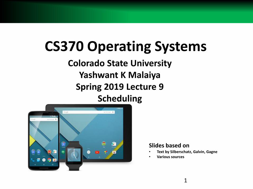
Questions from last time
• Prediction of next burst– Based on actual recent duration and predicted value (which is based on
past actual values)
– More recent data points get more weight (based on alpha).
– Why predict if you know the exact value?
– Computation time needed for prediction? vs typical burst time
• Does average wait time maters if the throughput is the same?
• Shortest Job First (SJF) vs Preemptive SJF– SJF is not preemptive
– Preemptive SJF (also termed Shortest remaining time first)
– A new process that will take shorter time will preempt a process with longer remaining time.
– Thus processes with a shorter remaining time have a higher priority.
• What system is responsible for preventing CPU from overheating?
3
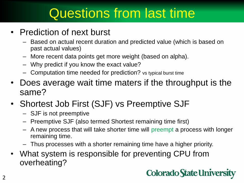
Scheduling Criteria
• CPU utilization – keep the CPU as busy as possible: Maximize
• Throughput – # of processes that complete their execution per time unit: Maximize
• Turnaround time –time to execute a process from submission to completion: Minimize
• Waiting time – amount of time a process has been waiting in the ready queue: Minimize
• Response time –time it takes from when a request was submitted until the first response is produced, not output (for time-sharing environment): Minimize
4
First- Come, First-Served (FCFS) Scheduling
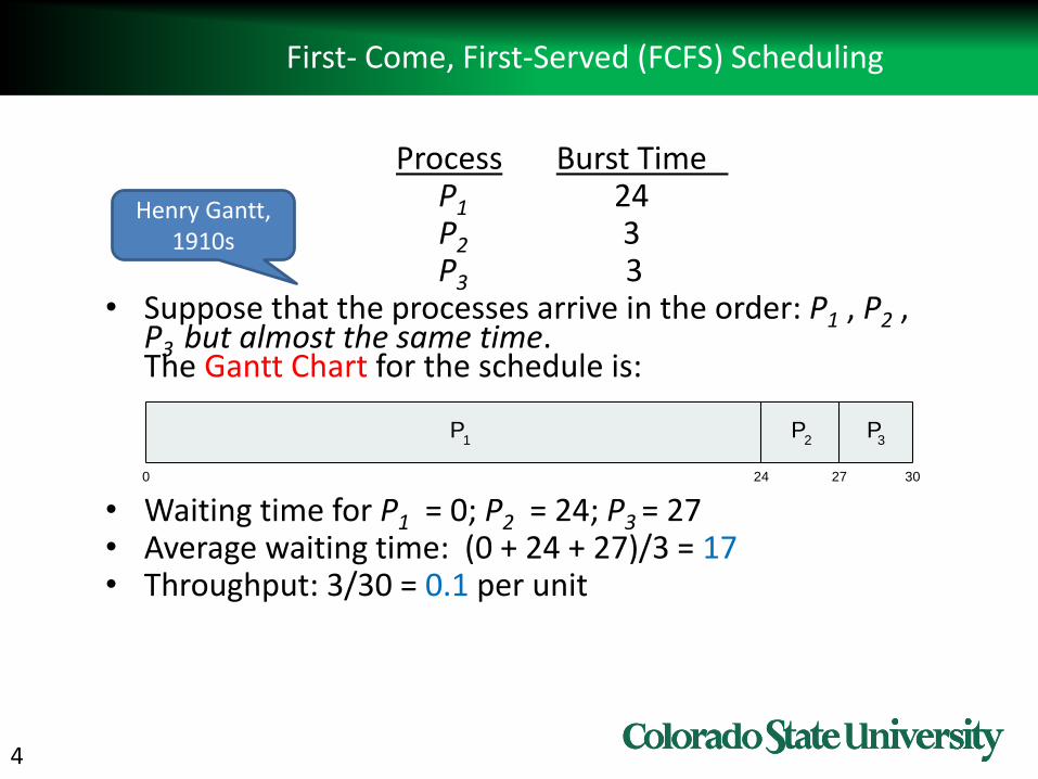
Process Burst TimeP1 24P2 3P3 3
• Suppose that the processes arrive in the order: P1 , P2 , P3 but almost the same time.The Gantt Chart for the schedule is:
• Waiting time for P1 = 0; P2 = 24; P3 = 27• Average waiting time: (0 + 24 + 27)/3 = 17• Throughput: 3/30 = 0.1 per unit
P P P1 2 3
0 24 3027
Henry Gantt, 1910s
5
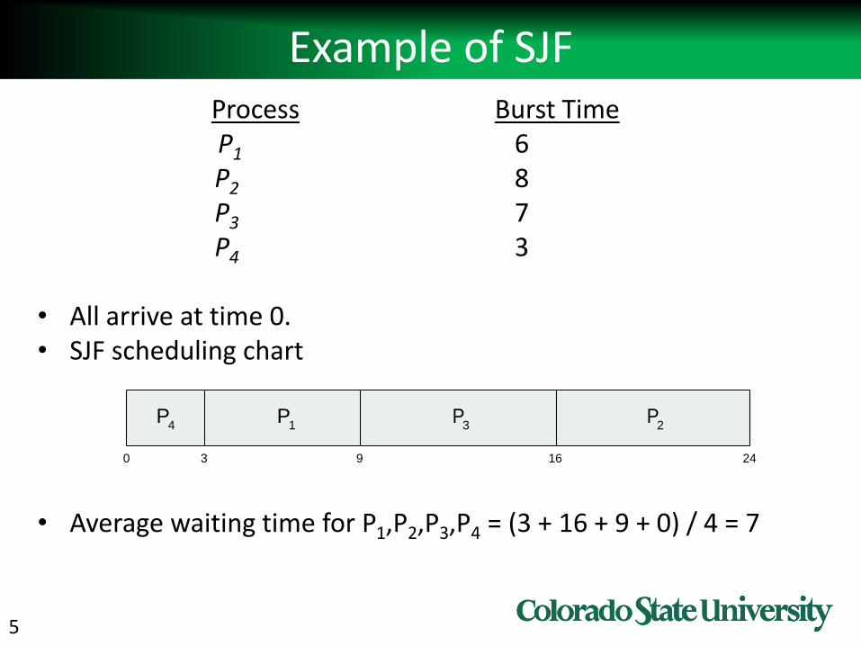
Example of SJFProcessArriva l TimeBurst TimeP1 0.0 6P2 2.0 8P3 4.0 7P4 5.0 3
• All arrive at time 0.• SJF scheduling chart
• Average waiting time for P1,P2,P3,P4 = (3 + 16 + 9 + 0) / 4 = 7
P3
0 3 24
P4
P1
169
P2
6
Determining Length of Next CPU Burst
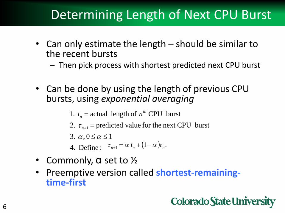
• Can only estimate the length – should be similar to the recent bursts– Then pick process with shortest predicted next CPU burst
• Can be done by using the length of previous CPU bursts, using exponential averaging
• Commonly, α set to ½• Preemptive version called shortest-remaining-
time-first
: Define4.
10 , 3.
burst CPUnext for the valuepredicted 2.
burst CPU of length actual 1.
1
n
th
n nt
.1 1 nnn t
7
Prediction of the Length of the Next CPU Burst
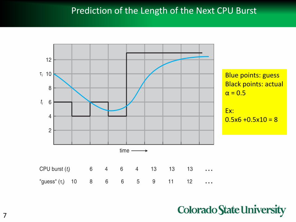
Blue points: guessBlack points: actualα = 0.5
Ex:0.5x6 +0.5x10 = 8
8
Shortest-remaining-time-first (preemptive SJF)
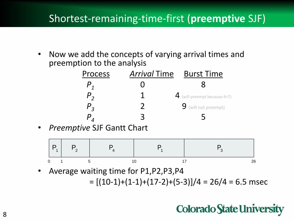
• Now we add the concepts of varying arrival times and preemption to the analysis
ProcessAarri Arrival TimeT Burst TimeP1 0 8P2 1 4 (will preempt because 4<7)
P3 2 9 (will not preempt)
P4 3 5• Preemptive SJF Gantt Chart
• Average waiting time for P1,P2,P3,P4= [(10-1)+(1-1)+(17-2)+(5-3)]/4 = 26/4 = 6.5 msec
P4
0 1 26
P1
P2
10
P3
P1
5 17
9
Priority Scheduling• A priority number (integer) is associated with each
process
• The CPU is allocated to the process with the highest priority (smallest integer highest priority)– Can be Preemptive (evict low priority process)
– Or Nonpreemptive
• SJF is priority scheduling where priority is the inverse of predicted next CPU burst time
• Problem Starvation – low priority processes may never execute
– Solution Aging – as time progresses increase the priority of the process
MIT had a low priority job waiting from 1967 to 1973 on IBM 7094!
10
Example of Priority Scheduling
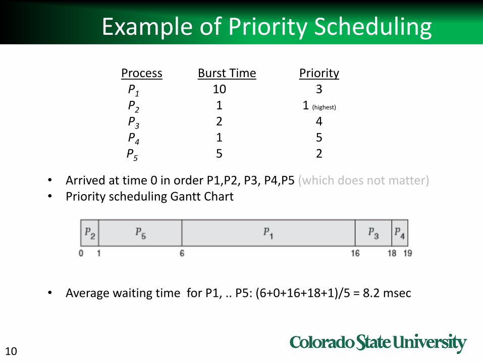
ProcessA arri Burst TimeT PriorityP1 10 3P2 1 1 (highest)
P3 2 4P4 1 5P5 5 2
• Arrived at time 0 in order P1,P2, P3, P4,P5 (which does not matter)• Priority scheduling Gantt Chart
• Average waiting time for P1, .. P5: (6+0+16+18+1)/5 = 8.2 msec
11
Round Robin (RR) with time quantum
• Each process gets a small unit of CPU time (time quantumq), usually 1-10 milliseconds. After this, the process is preempted, added to the end of the ready queue.
• If there are n processes in the ready queue and the time quantum is q, then each process gets 1/n of the CPU time in chunks of at most q time units at once. No process waits more than (n-1)q time units.
• Timer interrupts every quantum to schedule next process• Performance
– q large FIFO– q small q must be large with respect to context switch,
otherwise overhead is too high (overhead typically in 0.5% range)
12
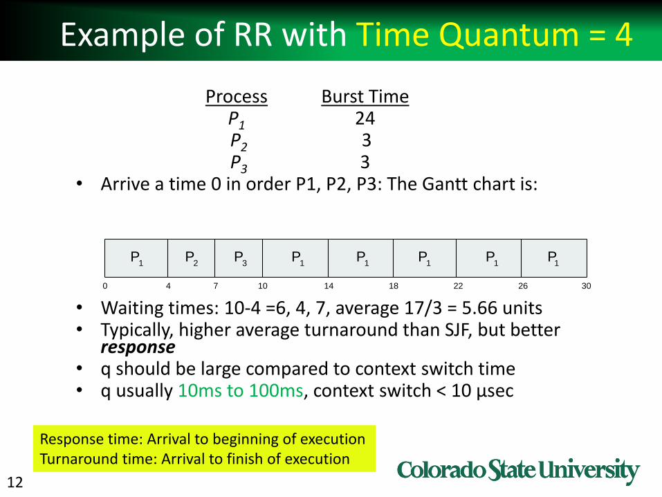
Example of RR with Time Quantum = 4
Process Burst TimeP1 24P2 3P3 3
• Arrive a time 0 in order P1, P2, P3: The Gantt chart is:
• Waiting times: 10-4 =6, 4, 7, average 17/3 = 5.66 units• Typically, higher average turnaround than SJF, but better
response• q should be large compared to context switch time• q usually 10ms to 100ms, context switch < 10 µsec
P P P1 1 1
0 18 3026144 7 10 22
P2
P3
P1
P1
P1
Response time: Arrival to beginning of executionTurnaround time: Arrival to finish of execution
13
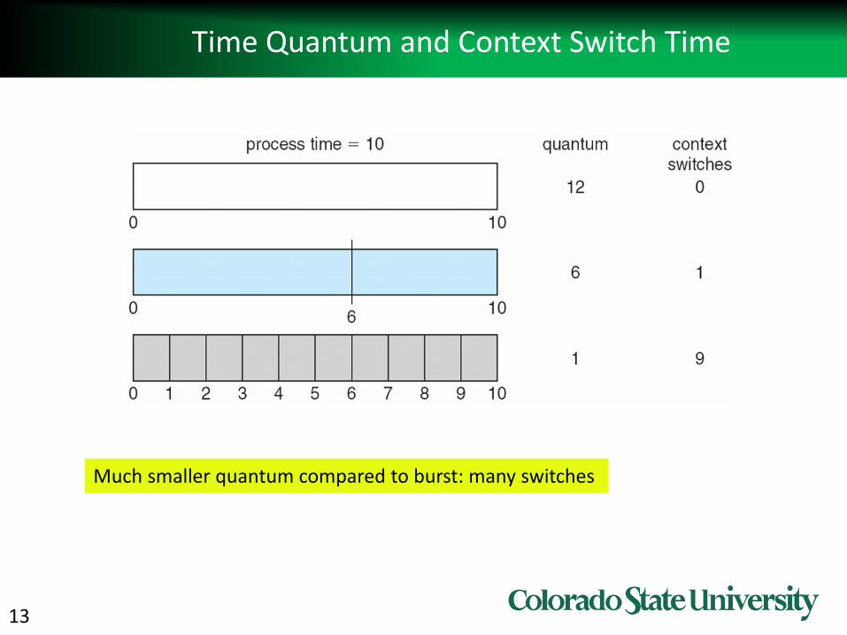
Time Quantum and Context Switch Time
Much smaller quantum compared to burst: many switches
14
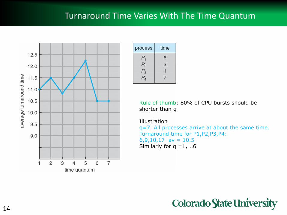
Turnaround Time Varies With The Time Quantum
Rule of thumb: 80% of CPU bursts should be shorter than q
Illustrationq=7. All processes arrive at about the same time.Turnaround time for P1,P2,P3,P4: 6,9,10,17 av = 10.5Similarly for q =1, ..6
15
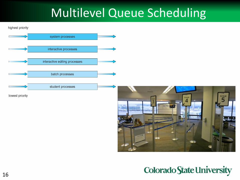
Multilevel Queue
• Ready queue is partitioned into separate queues, e.g.:– foreground (interactive)– background (batch)
• Process permanently in a given queue• Each queue has its own scheduling algorithm, e.g.:
– foreground – RR– background – FCFS
• Scheduling must be done between the queues:– Fixed priority scheduling; (i.e., serve all from foreground
then from background). Possibility of starvation. Or– Time slice – each queue gets a certain amount of CPU
time which it can schedule amongst its processes; i.e., 80% to foreground in RR, 20% to background in FCFS
16
Multilevel Queue Scheduling
17
Multilevel Feedback Queue
• A process can move between the various queues; aging can be implemented this way
• Multilevel-feedback-queue scheduler defined by the following parameters:
– number of queues
– scheduling algorithms for each queue
– method used to determine when to upgrade a process
– method used to determine when to demote a process
– method used to determine which queue a process will enter when that process needs service
Inventor Corbato won the Touring award!
18
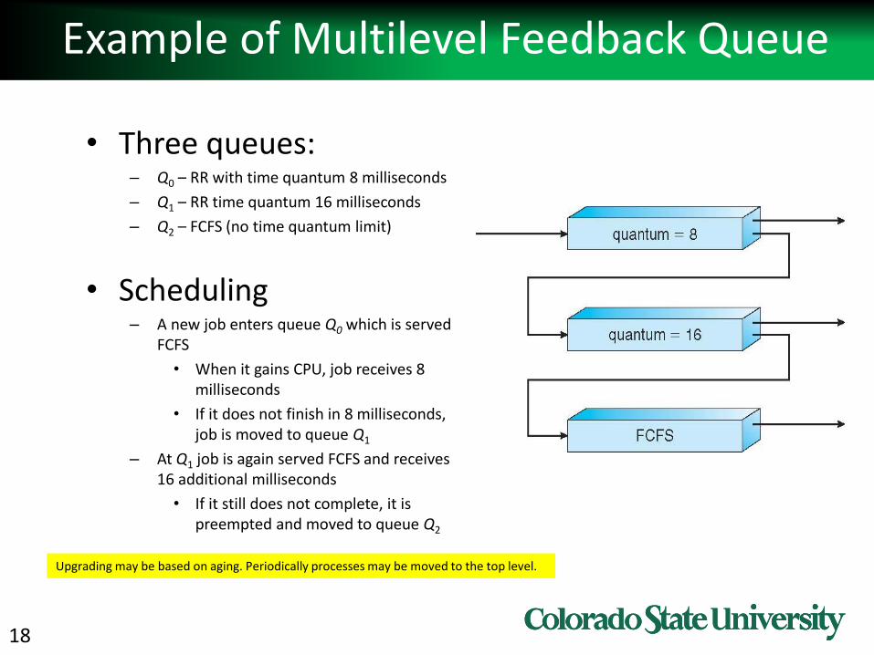
Example of Multilevel Feedback Queue
• Three queues: – Q0 – RR with time quantum 8 milliseconds
– Q1 – RR time quantum 16 milliseconds
– Q2 – FCFS (no time quantum limit)
• Scheduling– A new job enters queue Q0 which is served
FCFS
• When it gains CPU, job receives 8 milliseconds
• If it does not finish in 8 milliseconds, job is moved to queue Q1
– At Q1 job is again served FCFS and receives 16 additional milliseconds
• If it still does not complete, it is preempted and moved to queue Q2
Upgrading may be based on aging. Periodically processes may be moved to the top level.
19
Thread Scheduling
• Thread scheduling is similar• Distinction between user-level and kernel-level threads• When threads supported, threads scheduled, not processes
Scheduling competition• Many-to-one and many-to-many models, thread library schedules
user-level threads to run on LWP– Known as process-contention scope (PCS) since scheduling competition is
within the process– Typically done via priority set by programmer
• Kernel thread scheduled onto available CPU is system-contention scope (SCS) – competition among all threads in system
• Pthread API allows both, but Linux and Mac OSX allows only SCS.
LWP layer between kernel threads and user threads in some older OSs
20
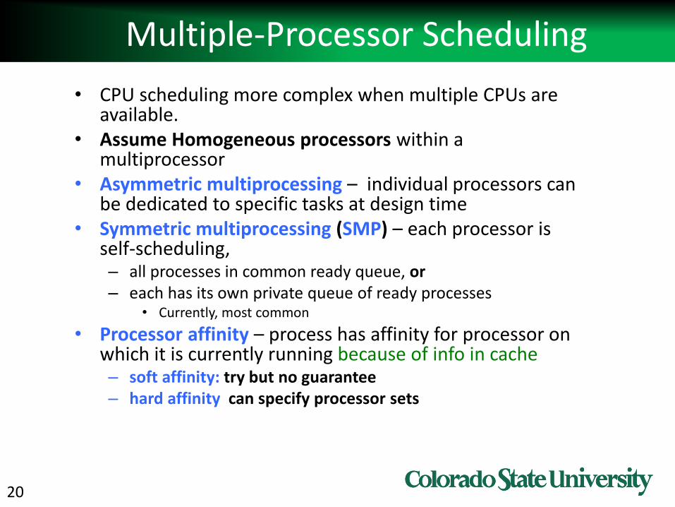
Multiple-Processor Scheduling
• CPU scheduling more complex when multiple CPUs are available.
• Assume Homogeneous processors within a multiprocessor
• Asymmetric multiprocessing – individual processors can be dedicated to specific tasks at design time
• Symmetric multiprocessing (SMP) – each processor is self-scheduling, – all processes in common ready queue, or– each has its own private queue of ready processes
• Currently, most common
• Processor affinity – process has affinity for processor on which it is currently running because of info in cache– soft affinity: try but no guarantee– hard affinity can specify processor sets
21
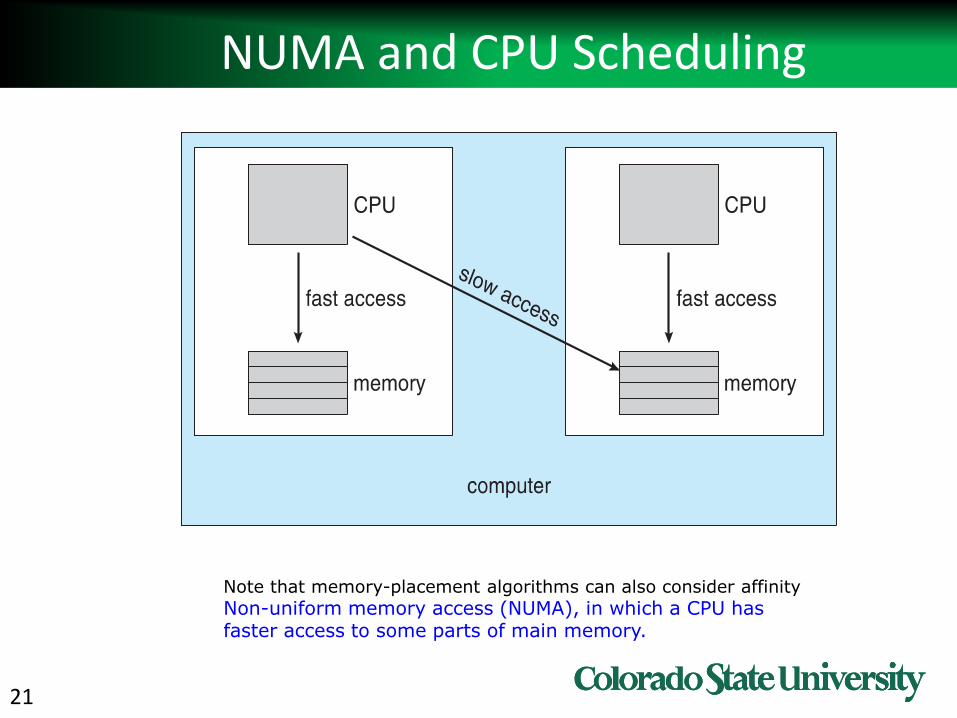
NUMA and CPU Scheduling
Note that memory-placement algorithms can also consider affinity
Non-uniform memory access (NUMA), in which a CPU has faster access to some parts of main memory.
22
Multiple-Processor Scheduling – Load Balancing
• If SMP, need to keep all CPUs loaded for efficiency
• Load balancing attempts to keep workload evenly distributed
– Push migration – periodic task checks load on each processor, and if found pushes task from overloaded CPU to other CPUs
– Pull migration – idle processors pulls waiting task from busy processor
– Combination of push/pull may be used.
23
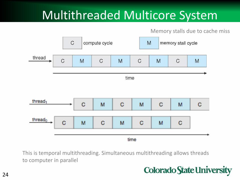
Multicore Processors
• Recent trend to place multiple processor cores on same physical chip
• Faster and consumes less power
• Multiple threads per core
– Takes advantage of memory stall to make progress on another thread while memory retrieve happens
– See next
24
Multithreaded Multicore System
This is temporal multithreading. Simultaneous multithreading allows threads to computer in parallel
Memory stalls due to cache miss
25
Real-Time CPU Scheduling
• Can present obvious challenges– Soft real-time systems – no guarantee as to when critical
real-time process will be scheduled– Hard real-time systems – task must be serviced by its
deadline
• For real-time scheduling, scheduler must support preemptive, priority-based scheduling– But only guarantees soft real-time
• For hard real-time must also provide ability to meet deadlines– periodic ones require CPU at constant intervals
26
Virtualization and Scheduling
• Virtualization software schedules multiple guests onto CPU(s)
• Each guest doing its own scheduling
– Not knowing it doesn’t own the CPUs
– Can effect time-of-day clocks in guests
• VMM has its own scheduler
• Various approaches have been used
– Workload aware, Guest OS cooperation, etc.
27
Operating System Examples
• Solaris scheduling: 6 classes, Inverse relationship between priorities and time quantum
• Windows XP scheduling: 32 priority levels (real-time, not real-time levels)
• Linux scheduling schemes have continued to evolve.
• Linux Completely fair scheduler (CFS, 2007): – Variable time-slice based on number and priority of the tasks in the
queue.
– Maximum execution time based on waiting processes (Q/n).
– Processes ready kept in a red-black binary tree with scheduling complexity of O(log N)
– Process with lowest weighted spent execution (virtual run time) time is picked next. VRN weighted by priority (“niceness”).
29
Algorithm Evaluation
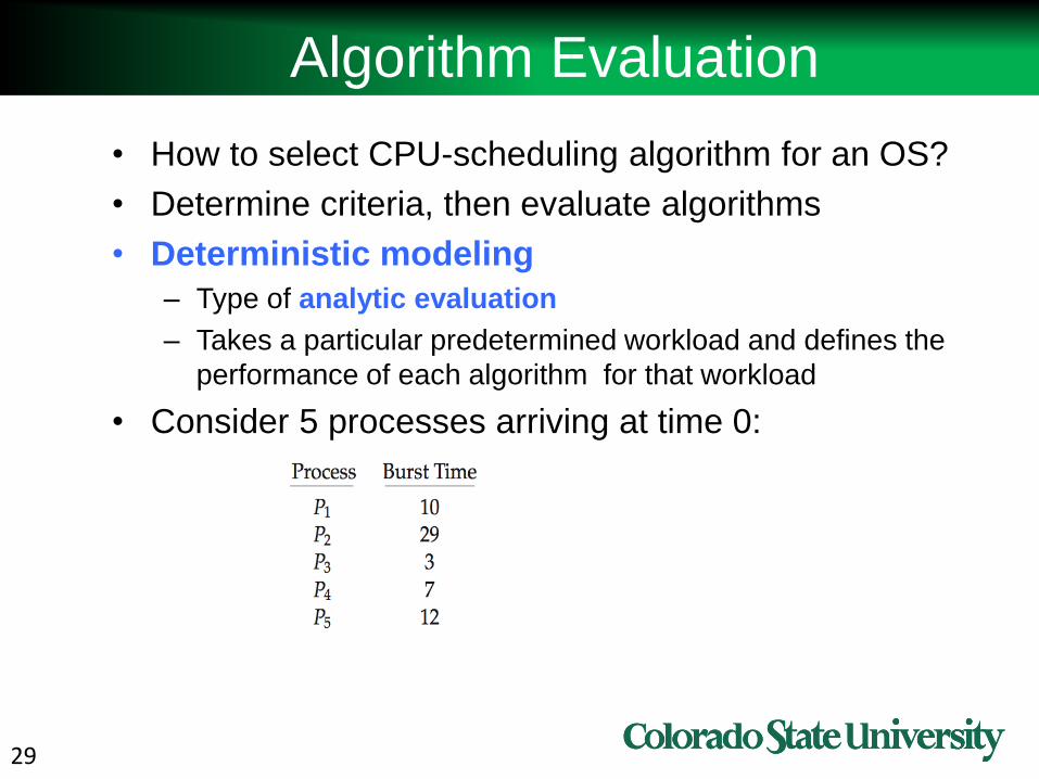
• How to select CPU-scheduling algorithm for an OS?
• Determine criteria, then evaluate algorithms
• Deterministic modeling
– Type of analytic evaluation
– Takes a particular predetermined workload and defines the
performance of each algorithm for that workload
• Consider 5 processes arriving at time 0:
30
Deterministic Evaluation
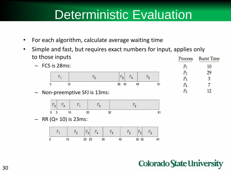
• For each algorithm, calculate average waiting time
• Simple and fast, but requires exact numbers for input, applies only to those inputs
– FCS is 28ms:
– Non-preemptive SFJ is 13ms:
– RR (Q= 10) is 23ms:
31
Probabilitistic Models
• Assume that the arrival of processes, and CPU
and I/O bursts are random
– Repeat deterministic evaluation for many random
cases and then average
• Approaches:
– Analytical: Queuing models
– Simulation: simulate using realistic assumptions
32
Queueing Models
• Describes the arrival of processes, and CPU
and I/O bursts probabilistically
– Commonly exponential, and described by mean
– Computes average throughput, utilization, waiting
time, etc
• Computer system described as network of
servers, each with queue of waiting
processes
– Knowing arrival rates and service rates
– Computes utilization, average queue length,
average wait time, etc
33
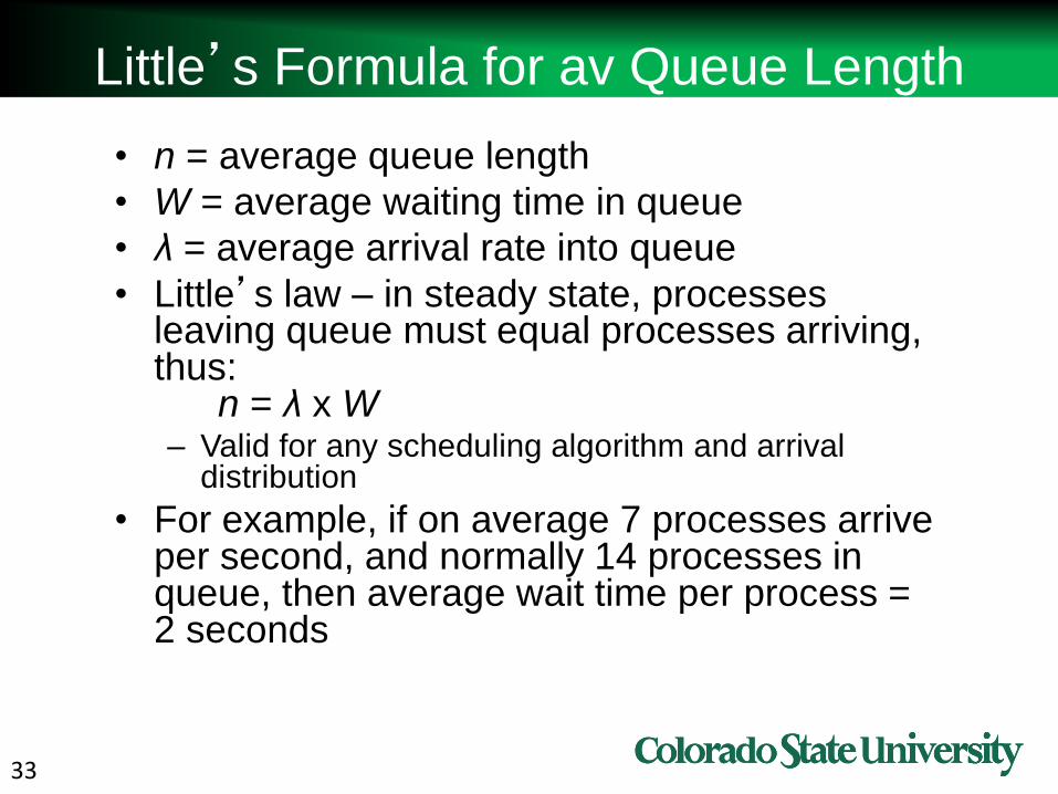
Little’s Formula for av Queue Length
• n = average queue length
• W = average waiting time in queue
• λ = average arrival rate into queue
• Little’s law – in steady state, processes leaving queue must equal processes arriving, thus:
n = λ x W– Valid for any scheduling algorithm and arrival
distribution
• For example, if on average 7 processes arrive per second, and normally 14 processes in queue, then average wait time per process = 2 seconds
34
Simulations
• Queueing models limited
• Simulations more accurate
– Programmed model of computer system
– Clock is a variable
– Gather statistics indicating algorithm performance
– Data to drive simulation gathered via
• Random number generator according to probabilities
• Distributions defined mathematically or empirically
• Trace tapes record sequences of real events in real systems

35
Evaluation of CPU Schedulers by Simulation
36
Implementation
Even simulations have limited accuracy
Just implement new scheduler and test in real systems
High cost, high risk
Environments vary
Most flexible schedulers can be modified per-site or per-system
Or APIs to modify priorities
But again environments vary
37 37
Colorado State UniversityYashwant K Malaiya
Spring 1018 Synchronization
CS370 Operating Systems
Slides based on • Text by Silberschatz, Galvin, Gagne• Various sources
38 38
Process Synchronization: Objectives
Concept of process synchronization.
The critical-section problem, whose solutions
can be used to ensure the consistency of shared
data
Software and hardware solutions of the critical-
section problem
Classical process-synchronization problems
Tools that are used to solve process
synchronization problems
39
Process Synchronization
EW Dijkstra Go To Statement Considered Harmful
40
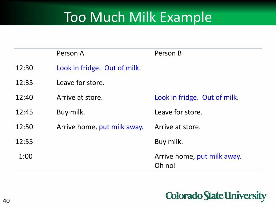
Too Much Milk Example
Person A Person B
12:30 Look in fridge. Out of milk.
12:35 Leave for store.
12:40 Arrive at store. Look in fridge. Out of milk.
12:45 Buy milk. Leave for store.
12:50 Arrive home, put milk away. Arrive at store.
12:55 Buy milk.
1:00 Arrive home, put milk away.Oh no!
41
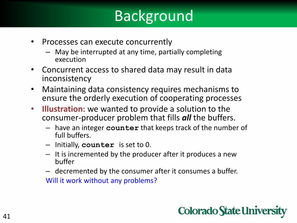
Background
• Processes can execute concurrently– May be interrupted at any time, partially completing
execution
• Concurrent access to shared data may result in data inconsistency
• Maintaining data consistency requires mechanisms to ensure the orderly execution of cooperating processes
• Illustration: we wanted to provide a solution to the consumer-producer problem that fills all the buffers. – have an integer counter that keeps track of the number of
full buffers. – Initially, counter is set to 0. – It is incremented by the producer after it produces a new
buffer – decremented by the consumer after it consumes a buffer.Will it work without any problems?
42
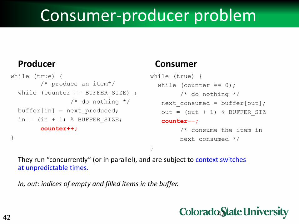
Consumer-producer problem
Producerwhile (true) {
/* produce an item*/
while (counter == BUFFER_SIZE) ;
/* do nothing */
buffer[in] = next_produced;
in = (in + 1) % BUFFER_SIZE;
counter++;
}
Consumerwhile (true) {
while (counter == 0);
/* do nothing */
next_consumed = buffer[out];
out = (out + 1) % BUFFER_SIZ
counter--;
/* consume the item in
next consumed */
}
42
They run “concurrently” (or in parallel), and are subject to context switches at unpredictable times.
In, out: indices of empty and filled items in the buffer.
43
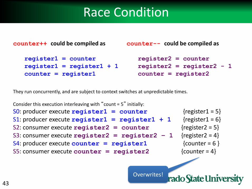
Race Condition
They run concurrently, and are subject to context switches at unpredictable times.
Consider this execution interleaving with “count = 5” initially:
S0: producer execute register1 = counter {register1 = 5}S1: producer execute register1 = register1 + 1 {register1 = 6}S2: consumer execute register2 = counter {register2 = 5} S3: consumer execute register2 = register2 – 1 {register2 = 4} S4: producer execute counter = register1 {counter = 6 } S5: consumer execute counter = register2 {counter = 4}
counter++ could be compiled as
register1 = counter
register1 = register1 + 1
counter = register1
counter-- could be compiled as
register2 = counter
register2 = register2 - 1
counter = register2
Overwrites!
44
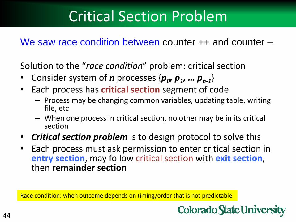
Critical Section Problem
We saw race condition between counter ++ and counter –
Solution to the “race condition” problem: critical section• Consider system of n processes {p0, p1, … pn-1}• Each process has critical section segment of code
– Process may be changing common variables, updating table, writing file, etc
– When one process in critical section, no other may be in its critical section
• Critical section problem is to design protocol to solve this• Each process must ask permission to enter critical section in
entry section, may follow critical section with exit section, then remainder section
Race condition: when outcome depends on timing/order that is not predictable