CS234 Notes - Lecture 2

Making Good Decisions Given a Model of the World

Rahul Sarkar, Emma Brunskill

March 20, 2018

3 Acting in a Markov decision process

We begin this lecture by recalling the de�nitions of a model, policy and value function for anagent. Let the agent's state and action spaces be denoted by S and A respectively. We then have thefollowing de�nitions:

• Model : A model is the mathematical description of the dynamics and rewards of the agent'senvironment, which includes the transition probabilities P (s′|s, a) of being in a successor states′ ∈ S when starting from a state s ∈ S and taking an action a ∈ A, and the rewards R(s, a)(either deterministic or stochastic) obtained by taking an action a ∈ A when in a state s ∈ S.

• Policy : A policy is a function π : S → A that maps the agent's states to actions. Policies canbe stochastic or deterministic.

• Value function : The value function V π corresponding to a particular policy π and for a states ∈ S, is the cumulative sum of future (discounted) rewards obtained by the agent, by startingfrom the state s and following the policy.

We also recall the notion of Markov property from the last lecture. Consider a stochastic process(s0, s1, s2, . . . ) evolving according to some transition dynamics. We say that the stochastic process hasthe Markov property if and only if P (si|s0, . . . , si−1) = P (si|si−1), ∀ i = 1, 2, . . . , i.e. the transitionprobability of the next state conditioned on the history including the current state is equal to thetransition probability of the next state conditioned only on the current state. In such a scenario, thecurrent state is a su�cient statistic of history of the stochastic process, and we say that �the future isindependent of the past given present.�

In this lecture, we will build on these de�nitions and proceed in order by �rst de�ning a Markovprocess (MP), followed by the de�nition of a Markov reward process (MRP) and �nally buildon both of them to de�ne a Markov decision process (MDP). We will �nish this lecture bydiscussing some algorithms which enable us to make good decisions when a MDP is completely known.

3.1 Markov process

In its most generality, a Markov process is a stochastic process that satis�es the Markov property,because of which we say that a Markov process is �memoryless�. For the purpose of this lecture, wewill make two additional assumptions that are very common in the reinforcement learning setting:

1

• Finite state space : The state space of the Markov process is �nite. This means that for theMarkov process (s0, s1, s2, . . . ), there is a state space S with |S| <∞, such that for all realizationsof the Markov process, we have si ∈ S for all i = 1, 2, . . . .

• Stationary transition probabilities : The transition probabilities are time independent. Mathe-matically, this means the following:

P (si = s′|si−1 = s) = P (sj = s′|sj−1 = s) , ∀ s, s′ ∈ S , ∀ i, j = 1, 2, . . . . (1)

Unless otherwise speci�ed, we will always assume that these two properties hold for any Markov processthat we will encounter in this lecture, including for any Markov reward process and any Markov decisionprocess to be de�ned later by adding progressively extra structure to the Markov process. Note that aMarkov process satisfying these assumptions is also sometimes called a �Markov chain�, although theprecise de�nition of a Markov chain varies.

For the Markov process, these assumptions lead to a nice characterization of the transition dynamicsin terms of a transition probability matrix P of size |S|×|S|, whose (i, j) entry is given by Pij = P (j|i),with i, j referring to the states of S ordered arbitrarily. It should be noted that the matrix P is anon-negative row-stochastic matrix, i.e. the sum of each row equals 1.

Henceforth, we will thus de�ne a Markov process by the tuple (S,P), which consists of the following:

• S : A �nite state space.

• P : A transition probability model that speci�es P (s′|s).

Exercise 3.1. (a) Prove that P is a row-stochastic matrix. (b) Show that 1 is an eigenvalue ofany row-stochastic matrix, and �nd a corresponding eigenvector. (c) Show that any eigenvalue of arow-stochastic matrix has maximum absolute value 1.

Exercise 3.2. The max-norm or in�nity-norm of a vector x ∈ Rn is denoted by ||x||∞, and de�nedas ||x||∞ = maxi |xi|, i.e. it is the component of x with the maximum absolute value. For any matrixA ∈ Rm×n, de�ne the following quantity

||A||∞ = supx∈Rn

x 6=0

||Ax||∞||x||∞

. (2)

(a) Prove that ||A||∞ satis�es all the properties of a norm. The quantity so de�ned is called the�induced in�nity norm� of a matrix.

(b) Prove that

||A||∞ = maxi=1,...,m

n∑j=1

|Aij |

. (3)

(c) Conclude that if A is row-stochastic, then ||A||∞ = 1.

(d) Prove that for every x ∈ Rn, ||Ax||∞ ≤ ||A||∞||x||∞.

3.1.1 Example of a Markov process : Mars Rover

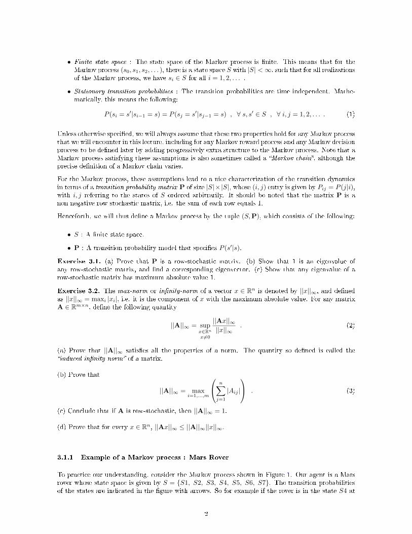
To practice our understanding, consider the Markov process shown in Figure 1. Our agent is a Marsrover whose state space is given by S = {S1, S2, S3, S4, S5, S6, S7}. The transition probabilitiesof the states are indicated in the �gure with arrows. So for example if the rover is in the state S4 at

2

Figure 1: Mars Rover Markov process.

the current time step, in the next time step it can go to the states S3, S4, S5 with probabilities givenby 0.4, 0.2, 0.4 respectively.

Assuming that the rover starts out in state S4, some possible episodes of the Markov process couldlook as follows:

� S4, S5, S6, S7, S7, S7, . . .

� S4, S4, S5, S4, S5, S6, . . .

� S4, S3, S2, S1, . . .

Exercise 3.3. Consider the example of a Markov process given in Figure 1. (a) Write down thetransition probability matrix for the Markov process.

3.2 Markov reward process

A Markov reward process is a Markov process, together with the speci�cation of a reward functionand a discount factor. It is formally represented using the tuple (S,P, R, γ) which are listed below:

• S : A �nite state space.

• P : A transition probability model that speci�es P (s′|s).

• R : A reward function that maps states to rewards (real numbers), i.e R : S → R.

• γ: Discount factor between 0 and 1.

We have already explained the roles played by S and P in the context of a Markov process. We willnext explain the concept of the reward function R and the discount factor γ, which are speci�c tothe Markov reward process. Additionally, we will also de�ne and explain a few quantities which areimportant in this context, such as the horizon, return and state value function of a Markov rewardprocess.

3.2.1 Reward function

In a Markov reward process, whenever a transition happens from a current state s to a successor states′, a reward is obtained depending on the current state s. Thus for the Markov process (s0, s1, s2, . . . ),each transition si → si+1 is accompanied by a reward ri for all i = 0, 1, . . . , and so a particular episode

3

of the Markov reward process is represented as (s0, r0, s1, r1, s2, r2, . . . ). We should note that theserewards can be either deterministic or stochastic. For a state s ∈ S, we de�ne the expected rewardR(s) by:

R(s) = E[r0|s0 = s], (4)

that is R(s) is the expected reward obtained during the �rst transition, when the Markov processstarts in state s. Just like the assumption of stationary transition probabilities, going forward we willalso assume the following:

• Stationary rewards : The rewards in a Markov reward process are stationary which means thatthey are time independent. In the deterministic case, mathematically this means that for allrealizations of the process we must have that:

ri = rj , whenever si = sj ∀ i, j = 0, 1, . . . , (5)

while in the case of stochastic rewards we require that the cumulative distribution functions(cdf) of the rewards conditioned on the current state be time independent. This is writtenmathematically as:

F (ri|si = s) = F (rj |sj = s) , ∀ s ∈ S , ∀ i, j = 0, 1, . . . , (6)

where F (ri|si = s) denotes the cdf of ri conditioned on the state si = s. Notice that as aconsequence of (5) and (6), we furthermore have the following result about the expected rewards:

R(s) = E[ri|si = s] , ∀ i = 0, 1, . . . . (7)

We will see that as long as the �stationary rewards� assumption is true about a Markov reward process,only the expected reward R matters in the things that we will be interested in, and we can deposeof the quantities ri entirely. Hence going forward, the word �reward� will be used interchangeably tomean both R and ri, and should be easily understood from context. Finally notice that R can berepresented as a vector of dimension |S|, in the case of a �nite state space S.

Exercise 3.4. (a) Under the assumptions of stationary transition probabilities and rewards, proveequation (7).

3.2.2 Horizon, Return and Value function

We next de�ne the notions of the horizon, return and value function for a Markov reward process.

• Horizon : The horizon H of a Markov reward process is de�ned as the number of time steps ineach episode (realization) of the process. The horizon can be �nite or in�nite. If the horizon is�nite, then the process is also called a �nite Markov reward process.

• Return : The return Gt of a Markov reward process is de�ned as the discounted sum of rewardsstarting at time t up to the horizon H, and is given by the following mathematical formula:

Gt =

H−1∑i=t

γi−tri , ∀ 0 ≤ t ≤ H − 1. (8)

• State value function : The state value function Vt(s) for a Markov reward process and a states ∈ S is de�ned as the expected return starting from state s at time t, and is given by thefollowing expression:

Vt(s) = E[Gt|st = s]. (9)

Notice that when the horizon H is in�nite, this de�nition (9) together with the stationaryassumptions of the rewards and transition probabilities imply that Vi(s) = Vj(s) for all i, j =0, 1, . . . , and thus in this case we will de�ne:

V (s) = V0(s) . (10)

4

Exercise 3.5. (a) If the assumptions of stationary transition probabilities and stationary rewardshold, and if the horizon H is in�nite, then using the de�nitions in (8) and (9) prove that Vi(s) = Vj(s)for all i, j = 0, 1, . . . .

3.2.3 Discount factor

Notice that in the de�nition of return Gt in (8), if the horizon is in�nite and γ = 1, then the returncan become in�nite even if the rewards are all bounded. If this happens, then the value functionV (s) can also become in�nite. Such problems cannot then be solved using a computer. To avoidsuch mathematical di�culties and make the problems computationally tractable we set γ < 1, whichexponentially weighs down the contribution of rewards at future times, in the calculation of the returnin (8). This quantity γ is called the discount factor. Other than for purely computational reasons,it should be noted that humans behave in much the same way - we tend to put more importance inimmediate rewards over rewards obtained at a later time. The interpretation of γ is that when γ = 0,we only care about the immediate reward, while when γ = 1, we put as much importance on futurerewards as compared the present. Finally, notice that if the horizon of the Markov reward process is�nite, i.e. H <∞, then we can set γ = 1, as the returns and value functions are always �nite.

Exercise 3.6. Consider a �nite horizon Markov reward process, with bounded rewards. Speci�callyassume that ∃M ∈ (0,∞) such that |ri| ≤M ∀ i and across all episodes (realizations). (a) Show thatthe return for any episode Gt as de�ned in (8) is bounded. (b) Can you suggest a bound? Speci�callycan you �nd C(M,γ, t,H) such that |Gt| ≤ C for any episode?

Exercise 3.7. Consider an in�nite horizon Markov reward process, with bounded rewards and γ < 1.(a) Prove that the return for any episode Gt as de�ned in (8) converges to a �nite limit. Hint: Consider

the partial sums SN =∑Ni=t γ

i−tri for N ≥ t. Show that {SN}N≥t is a Cauchy sequence.

3.2.4 Example of a Markov reward process : Mars Rover

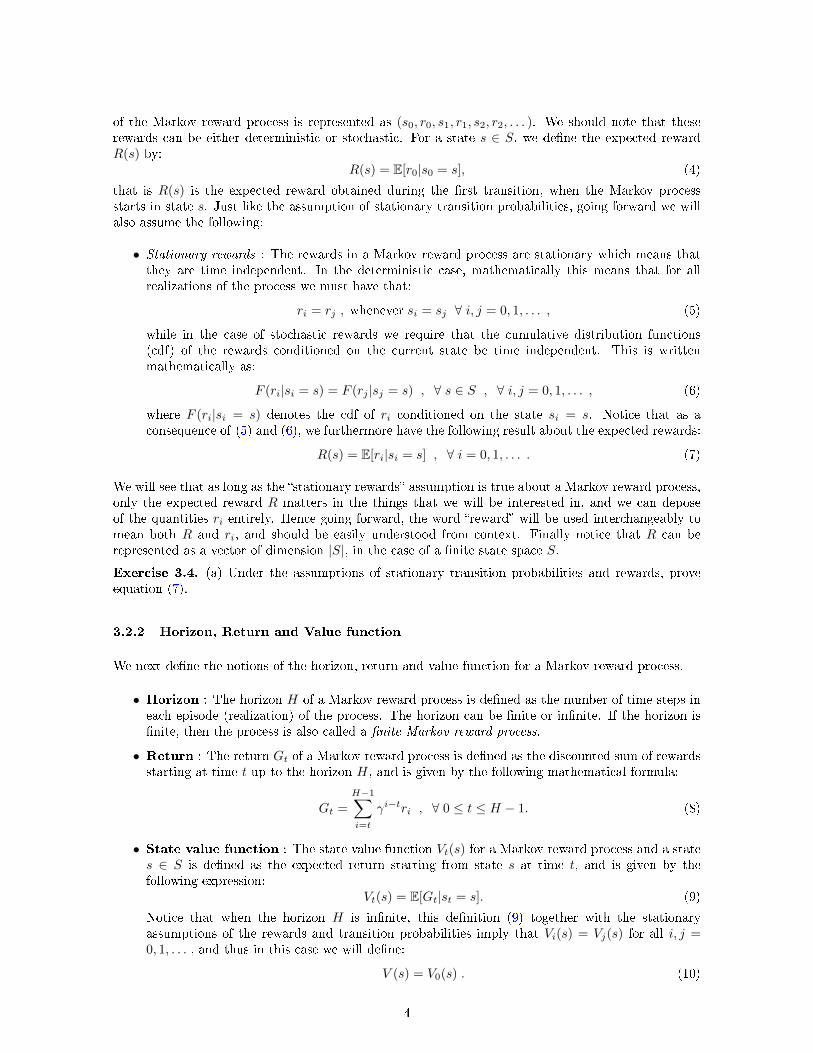
As an example, consider the Markov reward process in Figure 2. The states and the transition proba-bilities of this process are exactly the same as in the Mars rover Markov process example of Exercise3.3. The rewards obtained by executing an action from any of the states {S2, S3, S4, S5, S6} is 0,while any moves from states S1, S7 yield rewards 1, 10 respectively. The rewards are stationary anddeterministic. Assume γ = 0.5 in this example.

For illustration, let us again assume that the rover is initially in state S4. Consider the case when thehorizon is �nite : H = 4. A few possible episodes in this case with the return G0 in each case are givenbelow:

� S4, S5, S6, S7, S7 : G0 = 0 + 0.5 ∗ 0 + 0.52 ∗ 0 + 0.53 ∗ 10 = 1.25

� S4, S4, S5, S4, S5 : G0 = 0 + 0.5 ∗ 0 + 0.52 ∗ 0 + 0.53 ∗ 0 = 0

� S4, S3, S2, S1, S2 : G0 = 0 + 0.5 ∗ 0 + 0.52 ∗ 0 + 0.53 ∗ 1 = 0.125

3.3 Computing the value function of a Markov reward process

In this section we give three di�erent ways to compute the value function of a Markov reward process:

• Simulation

• Analytic solution

• Iterative solution

5

Figure 2: Mars Rover Markov reward process.

3.3.1 Monte Carlo simulation

The �rst method involves generating a large number of episodes using the transition probability modeland rewards of the Markov reward process. For each episode, the returns can be calculated whichcan then be averaged to give the average returns. Concentration inequalities bound how quickly theaverages concentrate to the mean value. For a Markov reward process M = (S,P, R, γ), state s, timet, and the number of simulation episodes N , the pseudo-code of the simulation algorithm is given inAlgorithm 1.

Algorithm 1 Monte Carlo simulation to calculate MRP value function

1: procedure Monte Carlo Evaluation(M, s, t,N)2: i← 03: Gt ← 04: while i 6= N do5: Generate an episode, starting from state s and time t6: Using the generated episode, calculate return g ←

∑H−1i=t γi−tri

7: Gt ← Gt + g8: i← i+ 1

9: Vt(s)← Gt/N10: return Vt(s)

3.3.2 Analytic solution

This method works only for an in�nite horizon Markov reward processes with γ < 1. Using (9), thefact that the horizon is inifnite, and using the stationary Markov property we have for any state s ∈ S:

V (s)(a)= V0(s) = E[G0|s0 = s] = E

[ ∞∑i=0

γiri

∣∣∣∣s0 = s

]= E[r0|s0 = s] +

∞∑i=1

γiE[ri|s0 = s]

(b)= E[r0|s0 = s] +

∞∑i=1

γi

(∑s′∈S

P (s1 = s′|s0 = s)E[ri|s0 = s, s1 = s′]

)(c)= E[r0|s0 = s] + γ

∑s′∈S

P (s′|s)E

[ ∞∑i=0

γiri

∣∣∣∣s0 = s′

](d)= R(s) + γ

∑s′∈S

P (s′|s)V (s′) ,

(11)

6

where (a) follows from (8), (9), and (10), (b) follows by the law of total expectation, (c) follows fromthe Markov property and due to stationarity, and (d) follows from (4). There is a nice interpretationof the �nal result of (11), namely that the �rst term R(s) is the immediate reward while the secondterm γ

∑s′∈S P (s′|s)V (s′) is the discounted sum of future rewards. The value function V (s) is the

sum of these two quantities. As |S| <∞, it is possible to write this equation in matrix form as:

V = R+ γPV , (12)

where P is the transition probability matrix introduced earlier, and R and V are column vectors ofdimension |S| formed by stacking all the values R(s) and V (s) respectively, for all s ∈ S. Equation(12) can be rearranged to give (I − γP)V = R, which has an analytical solution V = (I − γP)−1R.Notice that as γ < 1 and P is row-stochastic, (I − γP) is non-singular and hence can be inverted.Thus (12) always has a solution and the solution is unique. However, the computational cost of theanalytical method is O(|S|3), as it involves a matrix inverse and hence it is completely unsuitable forcases where the state space is very large.

Exercise 3.8. Consider the matrix (I− γP). (a) Show that 1− γ is an eigenvalue of this matrix, and�nd a corresponding eigenvector. (b) For 0 < γ < 1, use the result of Exercise 3.1 to conclude that(I− γP) is non-singular, and thus invertible.

Exercise 3.9. Consider the Markov reward process introduced in the example in section 3.2.4. (a) Ifthe horizon H is in�nite, calculate the value function for all the states.

3.3.3 Iterative solution

We now give an iterative solution to evaluate the value function in the in�nite horizon case (withγ < 1) and a dynamic programming based solution for the �nite horizon case. The surprising thingis that both the algorithms look surprisingly similar, to the point that it is hard to tell the di�erence.We �rst consider the �nite horizon case. It is easy to prove (by following almost exactly the sameproof of (11)) that the analog of equation (11) in the �nite horizon case is given by:

Vt(s) = R(s) + γ∑s′∈S

P (s′|s)Vt+1(s′) , ∀ t = 0, . . . ,H − 1,

VH(s) = 0 .

(13)

Exercise 3.10. Prove equations (13) for a �nite horizon Markov reward process.

These equations immediately lend themselves to a dynamic programming solution whose pseudo-codeis outlined in Algorithm 2. The algorithm takes as input a �nite horizon Markov reward processM = (S,P, R, γ), and computes the value function for all states and at all times.

Algorithm 2 Dynamic programming algorithm to calculate �nite MRP value function

1: procedure Dynamic Programming Value Function Evaluation(M)2: For all states s ∈ S, VH(s)← 03: t← H − 14: while t ≥ 0 do5: For all states s ∈ S, Vt(s) = R(s) + γ

∑s′∈S P (s′|s)Vt+1(s′)

6: t← t− 1

7: return Vt(s) for all s ∈ S and t = 0, . . . ,H

Let us now look at the iterative algorithm for the in�nite horizon case with γ < 1. The pseudo-codefor this algorithm is presented in Algorithm 3. The algorithm takes as input a Markov reward processM = (S,P, R, γ), and a tolerance ε, and computes the value function for all states.

7

Algorithm 3 Iterative algorithm to calculate MRP value function

1: procedure Iterative Value Function Evaluation(M, ε)2: For all states s ∈ S, V ′(s)← 0, V (s)←∞3: while ||V − V ′||∞ > ε do4: V ← V ′

5: For all states s ∈ S, V ′(s) = R(s) + γ∑s′∈S P (s′|s)V (s′)

6: return V ′(s) for all s ∈ S

For both these algorithms 2 and 3, the computational cost of each loop is O(|S|2). This is an improve-ment over the O(|S|3) cost of the analytical method in the ini�nite horizon case, however one mayneed quite a few iterations to converge depending on the tolerance level ε.

While the proof of correctness of algorithm 2 in the �nite horizon case is obvious, for the in�nitehorizon case it is not so clear if algorithm 3 always converges, and if it does whether it converges tothe correct solution (I− γP)−1R. The answers to both these questions are a�rmative as is shown bythe following theorem.

Theorem 3.1. Algorithm 3 always terminates. Moreover, if the output of the algorithm is V ′ and wedenote the true solution as V = (I− γP)−1R, then we have the error estimate ||V ′ − V ||∞ ≤ εγ

1−γ .

Proof. We consider the vector space R|S| equipped with the || · ||∞ norm (see Exercise 3.2), and recallthat R|S| so constructed is a Banach space (see Section A for a discussion on normed vector spaces).We start by noticing that both V and all the iterates of algorithm 3 are elements of R|S|.

De�ne the operator B : R|S| → R|S| (also known as the �Bellman backup� operator) that acts on anelement U ∈ R|S| as follows

(BU)(s) = R(s) + γ∑s′∈S

P (s′|s)U(s′) , ∀ s ∈ S, (14)

which can be written in compact matrix-vector notation as

BU = R+ γPU . (15)

We �rst prove that the operator B is a strict contraction (de�ned in De�nition A.3). For everyU1, U2 ∈ R|S|, using (15) we have

||BU1 −BU2||∞ = γ||PU1 −PU2||∞ = γ||P(U1 − U2)||∞≤ γ||P||∞||U1 − U2||∞ = γ||U1 − U2||∞ ,

(16)

where the second step follows by Exercise 3.2, and thus as 0 < γ < 1, we conclude that B is a strictcontraction on R|S|. Thus by the contraction mapping theorem (Theorem A.5), we conclude that Bhas a unique �xed point. From (15) and (12) it also follows that BV = R + γPV = V , and hence Vis a �xed point of B, and hence by uniqueness it must also be the only �xed point.

We next consider the iterates produced by algorithm 3 (if it is not allowed to terminate) and denotethem by {Vk}k≥1. Notice that these iterates satisfy the following relations

Vk =

{0 if k = 1,

BVk−1 if k > 1. (17)

By Theorem A.5, we further conclude that {Vk}k≥1 is a Cauchy sequence, and hence by De�nitionA.1 we conclude that ∃ N ≥ 1, such that ||Vm − Vn||∞ < ε for all m,n > N . This completes theproof that algorithm 3 terminates. Notice that the contraction mapping theorem (Theorem A.5) alsoimplies that Vk → V (see De�nition A.2 for exact notion of convergence).

8

To prove the error bound when the algorithm terminates, let the algorithm terminate after k iterations,and so the last iterate is Vk+1. We then have ||Vk+1 − Vk||∞ ≤ ε. Then using the triangle inequalityand the fact that Vk+1 = BVk we get,

||Vk − V ||∞ ≤ ||Vk − Vk+1||∞ + ||Vk+1 − V ||∞ = ||Vk − Vk+1||∞ + ||BVk −BV ||∞≤ ||Vk − Vk+1||∞ + γ||Vk − V ||∞ = ε+ γ||Vk − V ||∞ ,

(18)

and so ||Vk − V ||∞ ≤ ε1−γ . This �nally allows us to conclude that

||Vk+1 − V ||∞ = ||BVk −BV ||∞ ≤ γ||Vk − V ||∞ ≤εγ

1− γ. (19)

Exercise 3.11. Suppose that in algorithm 3, the initialization step is changed so V ′ is set randomly(all entries �nite), instead of V ′ ← 0. (a) Will the algorithm still converge? (b) Does the algorithmstill retain the same error estimate of Theorem 3.1 ?

Exercise 3.12. Suppose the assumptions of Theorem 3.1 hold. Using the same notations as in thetheorem prove the following:(a) For all k ≥ 1, ||Vk − V ||∞ ≤ γk−1||V ||∞ .(b) ||V2||∞ ≤ (1 + γ)||V ||∞ .(c) For all m,n ≥ 1, ||Vm − Vn||∞ ≤ (γm−1 + γn−1)||V ||∞ .

3.4 Markov decision process

We are now in a position to de�ne a Markov decision process (MDP). A MDP inherits the basic struc-ture of a Markov reward process with some important key di�erences, together with the speci�cationof a set of actions that an agent can take from each state. It is formally represented using the tuple(S,A, P,R, γ) which are listed below:

• S : A �nite state space.

• A : A �nite set of actions which are available from each state s.

• P : A transition probability model that speci�es P (s′|s, a).

• R : A reward function that maps a state-action pair to rewards (real numbers), i.e. R : S×A→ R.

• γ: Discount factor γ ∈ [0, 1].

Some of these quantities have been explained in the context of a Markov reward process. However inthe context of a MDP, there are important di�erences that we need to mention. The basic model ofthe dynamics is that there is a state space S, and an action space A, both of which we will considerto be �nite. The agent starts from a state si at time i, chooses an action ai from the action space,obtains a reward ri and then reaches a successor state si+1. An episode of a MDP is thus representedas (s0, a0, r0, s1, a1, r1, s2, a2, r2, . . . ).

Unlike in the case of a Markov process or a Markov reward process where the transition probabilitywas only a function of the successor state and the current state, in the case of a MDP the transitionprobabilities at time i are a function of the successor state si+1 along with both the current statesi and the action ai, written as P (si+1|si, ai). We still assume the principle of stationary transitionprobabilities which in the context of a MDP is written mathematically as

P (si = s′|si−1 = s, ai−1 = a) = P (sj = s′|sj−1 = s, aj−1 = a), (20)

9

for all s, s′ ∈ S, for all a ∈ A, and for all i, j = 1, 2, . . . .

The reward ri at time i depends on both si and ai in the case of a MDP, in contrast to a Markov rewardprocess where it depended only on the current state. These rewards can be stochastic or deterministic,but just like in the case of a Markov reward process, we will assume that the rewards are stationaryand the only relevant quantity will be the expected reward which we will denote by R(s, a) for a �xedstate s and action a, and de�ned below:

R(s, a) = E[ri|si = s, ai = a] , ∀ i = 0, 1, . . . . (21)

The notions of the discount factor γ, horizon H and return Gt for a MDP are exactly equivalentto those in the case of a Markov reward process. However the notion of a state value function isslightly modi�ed for a MDP as explained next.

3.4.1 MDP policies and policy evaluation

Given a MDP, a policy for the MDP speci�es what action to take in each state. A policy can eitherbe deterministic or stochastic. To cover both these cases, we will consider a policy to be a probabilitydistribution over actions given the current state. It is important to note that the policy may be varyingwith time, which is especially true in the case of �nite horizon MDPs. We will denote a generic policyby the boldface symbol π, de�ned as the in�nite dimensional tuple π = (π0, π1, . . . ), where πt refers tothe policy at time t. We will call policies that do not vary with time �stationary policies�, and indicatethem as π, i.e. in this case π = (π, π, . . . ). For a stationary policy π, if at time t the agent is in states, it will choose an action a with probability given by π(a|s) and this probability does not depend ont, while for a non-stationary policy the probability will depend on time t and we will be denoted byπt(a|s).

Given a policy π one can de�ne two quantities : the state value function and the state-action valuefunction for the MDP corresponding to the policy π, as shown below:

• State value function : The state value function V πt (s) for a state s ∈ S is de�ned as the

expected return starting from the state st = s at time t and following policy π, and is givenby the expression V π

t (s) = Eπ[Gt|st = s], where Eπ denotes that the expectation is taken withrespect to the policy π. Frequently we will drop the subscript π in the expectation to simplifynotation going forward. Thus E will mean expectation with respect to the policy unless speci�edotherwise, and so we can write

V πt (s) = E[Gt|st = s] . (22)

Notice that when the horizon H is in�nite, this de�nition (22) together with the stationaryassumptions of the rewards, transition probabilities and policy imply that for all s ∈ S, V π

i (s) =V πj (s) for all i, j = 0, 1, . . . , and thus in this case we will de�ne in a manner analogous to the

case of a Markov reward process:V π(s) = V π

0 (s) . (23)

• State-action value function : The state-action value function Qπt (s, a) for a state s and action

a is de�ned as the expected return starting from the state st = s at time t and taking the actionat = a, and then subsequently following the policy π. It is written mathematically as

Qπt (s, a) = E[Gt|st = s, at = a] . (24)

In the in�nite horizon case, similar to the state value function, the stationary assumptions aboutthe rewards, transition probabilities and policy imply that for all s ∈ S and a ∈ A, Qπ

i (s, a) =Qπj (s, a) for all i, j = 0, 1, . . . , which motivates the following de�nition

Qπ(s, a) = Qπ0 (s, a) . (25)

10

Exercise 3.13. Consider a stationary policy π = (π, π, . . . ). If the assumptions of stationary transi-tion probabilities and stationary rewards hold, and if the horizonH is in�nite, then using the de�nitionsin (22) and (24) prove that for all s ∈ S and a ∈ A, (a) V π

i (s) = V πj (s), and (b) Qπ

i (s, a) = Qπj (s, a)

for all i, j = 0, 1, . . . .

In the in�nite horizon case, the assumptions about stationary transition probabilities and rewardslead to the following important identity connecting the state value function and the state-action valuefunction for a stationary policy π :

Qπ(s, a)(a)= Qπ0 (s, a) = E[G0|s0 = s, a0 = a] = E

[ ∞∑i=0

γiri

∣∣∣∣s0 = s, a0 = a

]

= E[r0|s0 = s, a0 = a] +

∞∑i=1

γiE[ri|s0 = s, a0 = a]

(b)= R(s, a) +

∞∑i=1

γi

(∑s′∈S

P (s1 = s′|s0 = s, a0 = a)E[ri|s0 = s, a0 = a, s1 = s′]

)(c)= R(s, a) + γ

∑s′∈S

P (s′|s, a)

( ∞∑i=1

γi−1E[ri|s1 = s′]

)(d)= R(s, a) + γ

∑s′∈S

P (s′|s, a)V π(s′) ,

(26)

for all s ∈ S, a ∈ A, where (a) follows from (24) and (25), (b) is due to the law of total expectation,(c) follows from the Markov property, and (d) follows from Exercise 3.13 and linearity of expectation.

Exercise 3.14. Consider a policy π, not necessarily stationary. (a) Prove that in this case the analogof equation (26) is given by Qπ

t (s, a) = R(s, a) + γ∑s′∈S P (s′|s, a)V π

t+1(s′), for all s ∈ S, a ∈ A andfor all t = 0, 1, . . . .

An interesting aspect of specifying a stationary policy π on a MDP is that evaluating the value functionfor the policy is equivalent to evaluating the value function on an equivalent Markov reward process.Speci�cally we de�ne the Markov reward process M ′(S,Pπ, Rπ, γ), where Pπ and Rπ are given by:

Rπ(s) =∑a∈A

π(a|s)R(s, a) ,

Pπ(s′|s) =∑a∈A

π(a|s)P (s′|s, a) .(27)

Exercise 3.15. Consider a stationary policy π for a MDP. (a) Prove that the value function of thepolicy V π satis�es the identity V π(s) = Rπ(s) + γ

∑s′∈S P

π(s′|s)V π(s′) for all states s ∈ S, with Rπand Pπ de�ned by (27).

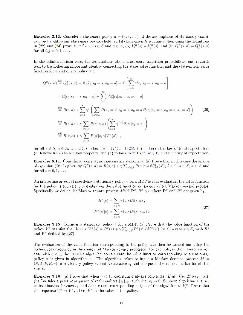
The evaluation of the value function corresponding to the policy can then be carried out using thetechniques introduced in the context of Markov reward processes. For example, in the in�nite horizoncase with γ < 1, the iterative algorithm to calculate the value function corresponding to a stationarypolicy π is given in algorithm 4. The algorithm takes as input a Markov decision process M =(S,A, P,R, γ), a stationary policy π, and a tolerance ε, and computes the value function for all thestates.

Exercise 3.16. (a) Prove that when γ < 1, algorithm 4 always converges. Hint: Use Theorem 3.1.(b) Consider a positive sequence of real numbers {εi}i≥1 such that εi → 0. Suppose algorithm 4 is runto termination for each εi, and denote each corresponding output of the algorithm as V πi . Prove thatthe sequence V πi → V π, where V π is the value of the policy.

11

Algorithm 4 Iterative algorithm to calculate MDP value function for a stationary policy π

1: procedure Policy Evaluation(M,π, ε)2: For all states s ∈ S, de�ne Rπ(s) =

∑a∈A π(a|s)R(s, a)

3: For all states s, s′ ∈ S, de�ne Pπ(s′|s) =∑a∈A π(a|s)P (s′|s, a)

4: For all states s ∈ S, V ′(s)← 0, V (s)←∞5: while ||V − V ′||∞ > ε do6: V ← V ′

7: For all states s ∈ S, V ′(s) = Rπ(s) + γ∑s′∈S P

π(s′|s)V (s′)

8: return V ′(s) for all s ∈ S

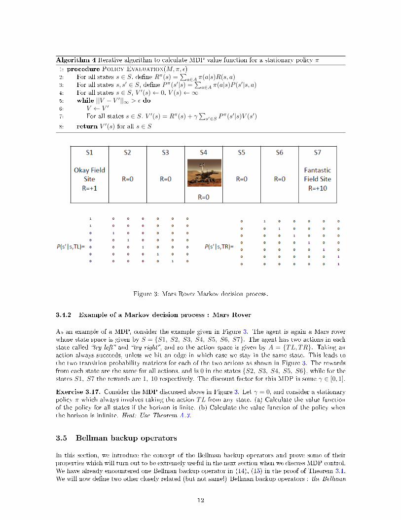
Figure 3: Mars Rover Markov decision process.

3.4.2 Example of a Markov decision process : Mars Rover

As an example of a MDP, consider the example given in Figure 3. The agent is again a Mars roverwhose state space is given by S = {S1, S2, S3, S4, S5, S6, S7}. The agent has two actions in eachstate called �try left� and �try right�, and so the action space is given by A = {TL, TR}. Taking anaction always succeeds, unless we hit an edge in which case we stay in the same state. This leads tothe two transition probability matrices for each of the two actions as shown in Figure 3. The rewardsfrom each state are the same for all actions, and is 0 in the states {S2, S3, S4, S5, S6}, while for thestates S1, S7 the rewards are 1, 10 respectively. The discount factor for this MDP is some γ ∈ [0, 1].

Exercise 3.17. Consider the MDP discussed above in Figure 3. Let γ = 0, and consider a stationarypolicy π which always involves taking the action TL from any state. (a) Calculate the value functionof the policy for all states if the horizon is �nite. (b) Calculate the value function of the policy whenthe horizon is in�nite. Hint: Use Theorem A.3.

3.5 Bellman backup operators

In this section, we introduce the concept of the Bellman backup operators and prove some of theirproperties which will turn out to be extremely useful in the next section when we discuss MDP control.We have already encountered one Bellman backup operator in (14), (15) in the proof of Theorem 3.1.We will now de�ne two other closely related (but not same!) Bellman backup operators : the Bellman

12

expectation backup operator and the Bellman optimality backup operator.

3.5.1 Bellman expectation backup operator

Suppose we are given a MDP M = (S,A, P,R, γ), and a stationary policy π which can be deter-ministic or stochastic. We have already seen in section 3.4.1 that this is equivalent to a MRPM ′ = (S, Pπ, Rπ, γ), where Pπ and Rπ are de�ned in (27). The value function of policy π evalu-ated on M , and denoted by V π, is the same as the value function evaluated on M ′, where we haveused the corresponding de�nitions of the value function for a MDP and MRP respectively. Note thatV π lives in the �nite dimensional Banach space R|S|, which we will equip with the in�nity norm || · ||∞introduced in Exercise 3.2.

Then for element U ∈ R|S| the Bellman expectation backup operator Bπ for the policy π is de�ned as

(BπU)(s) = Rπ(s) + γ∑s′∈S

Pπ(s′|s)U(s′) , ∀ s ∈ S . (28)

We should note that we have already seen this operator appear once before in algorithm 4. We nowprove some properties of this operator.

Theorem 3.2. The operator Bπ de�ned in (28) is a contraction map. If γ < 1 then it is a strictcontraction and has a unique �xed point.

Proof. Consider U1, U2 ∈ R|S|. Then for a state s ∈ S, we have from (28) and triangle inequality

|(BπU1)(s)− (BπU2)(s)| = γ

∣∣∣∣∣∑s′∈S

Pπ(s′|s)(U1(s′)− U2(s′))

∣∣∣∣∣ ≤ γ∑s′∈S

Pπ(s′|s)|U1(s′)− U2(s′)|

≤ γ∑s′∈S

Pπ(s′|s) maxs′′∈S

|U1(s′′)− U2(s′′)| = γ∑s′∈S

Pπ(s′|s) ||U1 − U2||∞

= γ ||U1 − U2||∞ .

(29)

As (29) is true for every s ∈ S we conclude that ||BπU1 − BπU2||∞ ≤ γ ||U1 − U2||∞, and hence Bπ

is a contraction map as γ ∈ [0, 1].

Considering γ < 1 in (29), we conclude that in this case Bπ is a strict contraction, and hence byapplying Theorem A.5 it has a unique �xed point.

Corollary 3.2.1. Let γ < 1. Then for any U ∈ R|S| the sequence {(Bπ)kU}k≥0 is a Cauchy sequenceand converges to the �xed point of Bπ.

Proof. The proof follows directly by applying Theorem 3.2, followed by Theorem A.4 and the contrac-tion mapping theorem (TheoremA.5).

This also implies that for a stationary policy π, the value function of the policy V π is a �xed point ofBπ, as shown by the following corollary.

Corollary 3.2.2. Let π be a policy for an in�nite horizon MDP with γ < 1. Then the value functionof the policy V π is a �xed point of Bπ.

Proof. The fact that (BπV π)(s) = V π(s) for all states s ∈ S, follows from the de�nition (28) of Bπ

and Exercise 3.15.

13

The next theorem proves the �monotonicity� property of the Bellman expectation backup operator.

Theorem 3.3. Suppose we have U1, U2 ∈ R|S| such that for all s ∈ S, U1(s) ≥ U2(s). Then for everystationary policy π, we have (BπU1)(s) ≥ (BπU2)(s) for all s ∈ S. If instead the inequality is strict,i.e. U1(s) > U2(s) for all s ∈ S, then we have (BπU1)(s) > (BπU2)(s) for all s ∈ S.

Proof. When U1(s) ≥ U2(s) for all s ∈ S, using de�nition (28) of Bπ we obtain,

(BπU1)(s)− (BπU2)(s) =∑s′∈S

Pπ(s′|s)(U1(s′)− U2(s′)) ≥ 0 , (30)

ans when U1(s) > U2(s) for all s ∈ S, the same steps give (BπU1)(s) − (BπU2)(s) > 0, for all statess ∈ S.

3.5.2 Bellman optimality backup operator

Suppose we are now given a MDP M = (S,A, P,R, γ). We again consider the �nite dimensionalBanach space R|S| equipped with the in�nity norm || · ||∞. Then for every element U ∈ R|S| theBellman optimality backup operator B∗ is de�ned as

(B∗U)(s) = maxa∈A

[R(s, a) + γ

∑s′∈S

P (s′|s, a)U(s′)

], ∀ s ∈ S . (31)

We next prove analogous properties for this operator which are similar to the ones for the Bellmanexpectation backup operator.

Theorem 3.4. For every U1, U2 ∈ R|S|, and for all states s ∈ S the following inequalities are true:

(a)

(B∗U1)(s)− (B∗U2)(s) ≤ γ maxa∈A

[∑s′∈S

P (s′|s, a) (U1(s′)− U2(s′))

]

≤ γ maxa∈A

[∑s′∈S

P (s′|s, a) |U1(s′)− U2(s′)|

],

(32)

(b)

|(B∗U1)(s)− (B∗U2)(s)| ≤ γ maxa∈A

[∑s′∈S

P (s′|s, a) |U1(s′)− U2(s′)|

]≤ γ ||U1 − U2||∞ . (33)

Proof. We �rst prove part (a). Fix a state s ∈ S. Using (31) and as the action space A is �nite, weconclude that there exists a1, a2 ∈ A, not necessarily di�erent, such that the following holds:

(B∗U1)(s) = R(s, a1) + γ∑s′∈S

P (s′|s, a1)U1(s′) ,

(B∗U2)(s) = R(s, a2) + γ∑s′∈S

P (s′|s, a2)U2(s′) .(34)

Then by the de�nition of maximum in (31), we also have for the action a1 that

(B∗U2)(s) ≥ R(s, a1) + γ∑s′∈S

P (s′|s, a1)U2(s′) . (35)

14

Thus from (34) and (35) we deduce the following

(B∗U1)(s)− (B∗U2)(s) ≤ γ∑s′∈S

P (s′|s, a1) (U1(s′)− U2(s′))

≤ γ maxa∈A

[∑s′∈S

P (s′|s, a) (U1(s′)− U2(s′))

],

(36)

which proves the �rst inequality of (a). For the second inequality notice that we have for all statess′ ∈ S, U1(s′) − U2(s′) ≤ |U1(s′) − U2(s′)|, and so multiplying each of these inequalities by positivenumbers P (s′|s, a) for some a ∈ A, and summing over all s′ gives∑

s′∈SP (s′|s, a) (U1(s′)− U2(s′)) ≤

∑s′∈S

P (s′|s, a) |(U1(s′)− U2(s′))| . (37)

The result is proved by taking the max over all a ∈ A, by using monotonicity of the max function.

To prove part (b), notice that by interchanging the roles of U1, U2, we have from part (a)

(B∗U2)(s)− (B∗U1)(s) ≤ γ maxa∈A

[∑s′∈S

P (s′|s, a) |U1(s′)− U2(s′)|

], (38)

and thus combining (38) and (32) we obtain

|(B∗U1)(s)− (B∗U2)(s)| ≤ γ maxa∈A

[∑s′∈S

P (s′|s, a) |U1(s′)− U2(s′)|

]

≤ γ maxa∈A

[∑s′∈S

P (s′|s, a) maxs′′∈S

|U1(s′′)− U2(s′′)|

]

= γ maxa∈A

[∑s′∈S

P (s′|s, a) ||U1 − U2||∞

]= γ max

a∈A||U1 − U2||∞ = γ ||U1 − U2||∞ ,

(39)

which proves (b).

Theorem 3.5. The operator B∗ de�ned in (31) is a contraction map. If γ < 1 then it is a strictcontraction and has a unique �xed point.

Proof. The fact that B∗ is a contraction follows from Theorem 3.4 by observing that (32) is true for alls ∈ S, and so must be true in particular for arg max

s∈S|(B∗U1)(s)− (B∗U2)(s)|, for every U1, U2 ∈ R|S|.

Thus ||B∗U1 −B∗U2||∞ ≤ γ ||U1 − U2||∞, proving that B∗ is a contraction map as γ ∈ [0, 1]. Settingγ < 1 in this inequality proves that B∗ is a strict contraction for γ ∈ [0, 1) and thus has a unique �xedpoint by Theorem A.5.

Corollary 3.5.1. Let γ < 1. Then for any U ∈ R|S| the sequence {(B∗)kU}k≥0 is a Cauchy sequenceand converges to the �xed point of B∗.

Proof. The proof follows directly by applying Theorem 3.5, followed by Theorem A.4 and the contrac-tion mapping theorem (TheoremA.5).

The next theorem compares the result of the application of Bπ versus B∗ to some U ∈ R|S|.

Theorem 3.6. For every stationary policy π, for every U ∈ R|S| and for all s ∈ S, (B∗U)(s) ≥(BπU)(s).

15

Proof. Fix a stationary policy π, and let Bπ be the corresponding Bellman expectation backup oper-ator. Fix some U ∈ R|S|. Let us also �x some s ∈ S. Then from de�nition (31) of B∗ we have

(B∗U)(s) = maxa∈A

[R(s, a) + γ

∑s′∈S

P (s′|s, a)U(s′)

]≥ R(s, a) +γ

∑s′∈S

P (s′|s, a)U(s′) , ∀ a ∈ A . (40)

Multiplying (40) by π(a|s) and summing over all a ∈ A gives

(B∗U)(s) =∑a∈A

π(a|s)(B∗U)(s) ≥∑a∈A

π(a|s)

[R(s, a) + γ

∑s′∈S

P (s′|s, a)U(s′)

]

=∑a∈A

π(a|s)R(s, a) + γ∑s′∈S

(∑a∈A

π(a|s)P (s′|s, a)

)U(s′)

= Rπ(s) + γ∑s′∈S

Pπ(s′|s)U(s′) = (BπU)(s) ,

(41)

where the last equality follows from de�nitions (27) and (28) of Rπ, Pπ and Bπ, thus proving thetheorem.

3.6 MDP control in the in�nite horizon setting

We now have all the background necessary to discuss the problem of �MDP control�, where we seekto �nd the best policy (often a policy), that achieves the greatest value function among the set of allpossible policies. In the context of reinforcement learning, this is precisely the objective of the agent.We are going to �rst discuss the in�nite horizon case in this section, and the �nite horizon case will bementioned in the next section. We do it this way because the in�nite horizon case is a much harderproblem, that presents quite a few mathematical challenges which will need to be resolved.

To get started, we need to address the question �what do we exactly mean by �nding an optimal policy?�. Precisely we want to know whether a policy always exists, which we will denote by π∗, whosevalue function is at least as good as the value function of any other policy. In other words, we need toensure that the supremum of the value function is actually attained for some policy ! To appreciate thesubtlety of this point, consider the example of maximizing the function f : R→ R on (0, 1) de�ned asf(x) = x, and note that this problem does not have a solution. But sup f(x) = 1, although @ x ∈ (0, 1)for which this is attained.

We �rst de�ne precisely what it means for a policy, not necessarily stationary, to be an optimalpolicy.

De�nition 3.1. A policy π∗ is an optimal policy i� for every policy π, for all t = 0, 1, . . . , and for allstates s ∈ S, V π∗

t (s) ≥ V πt (s).

The next result that we leave for the reader to prove states that for an in�nite horizon MDP, existenceof an optimal policy also implies the existence of a stationary optimal policy. This result is intuitivelyobvious, and is a very important result as it signi�cantly reduces the universe of policies to considerwhen searching for an optimal policy, if it exists. In particular, it states that we need only considerpolicies that are stationary.

Exercise 3.18. (a) Consider an in�nite horizon MDP. Let π∗ be an optimal policy for the MDP.Prove that there exists a stationary policy π, that is π = (π, π, . . . ), which is also optimal.

The next two theorems improve on the conclusion of Exercise 3.18 and show us that we may restrictthe search to a �nite set of deterministic stationary policies.

16

Theorem 3.7. The number of deterministic stationary policies is �nite, and equals |A||S|.

Proof. Since the policies are stationary and deterministic, each policy can be represented as a functionπ : S → A. The number of such distinct functions is given by |A||S|. This also proves that the set ofdeterministic stationary policies is �nite.

Theorem 3.8. If π is a stationary policy for an in�nite horizon MDP with γ < 1, then there existsa deterministic stationary policy π̂ such that V π̂(s) ≥ V π(s) for all states s ∈ S. One such policy isgiven by the stationary policy

π̂(s) = arg maxa∈A

[R(s, a) + γ

∑s′∈S

P (s′|s, a)V π(s′)

], ∀ s ∈ S , (42)

which satis�es the equality (Bπ̂V π)(s) = (B∗V π)(s) ≥ V π(s) for all s. Moreover V π̂(s) = V π(s) forall s, i� (B∗V π)(s) = V π(s) for all s.

Proof. We �rst notice that the policy π̂ de�ned in (42) is a stationary policy (by de�nition), and isalso deterministic for every s ∈ S, by the de�nition of arg max with ties broken randomly.

As π̂ is deterministic, we can conclude using (27) that Rπ̂(s) = R(s, π̂(s)) and P π̂(s′|s) = P (s′|s, π̂(s))for all s ∈ S and a ∈ A, and thus we have

(Bπ̂V π)(s) = R(s, π̂(s)) + γ∑s′∈S

P (s′|s, π̂(s))V π(s) = (B∗V π)(s) , (43)

for all states s ∈ S using (42), and the de�nitions of the Bellman backup operators in (28) and (31).Next, by Corollary 3.2.2 we have BπV π = V π, and by Theorem 3.6 we have B∗V π ≥ BπV π, and socombining these with (43) we obtain

(Bπ̂V π)(s) = (B∗V π)(s) ≥ V π(s) , ∀ s ∈ S . (44)

Next using Theorem 3.3, the monotonicity property of Bπ̂ allows us to conclude by repeatedly applyingBπ̂ to both sides of (44) that ((Bπ̂)kV π)(s) ≥ V π(s) for all k ≥ 1, and for all states s ∈ S. Then usingCorollary 3.2.1, and noticing that V π̂ is the unique �xed point of Bπ̂ we obtain by taking limits

V π̂(s) = (Bπ̂V π̂)(s) = limk→∞

((Bπ̂)kV π)(s) ≥ V π(s) , ∀ s ∈ S . (45)

To prove the second part of the theorem, �rst assume that B∗V π = V π. Then by (44) we haveBπ̂V π = B∗V π = V π, and so by uniqueness of the �xed point of Bπ̂ we get V π̂ = Bπ̂V π̂ = V π. Nextassume that V π̂ = V π. Then again by (44) we have V π = V π̂ = Bπ̂V π̂ = Bπ̂V π = B∗V π ≥ V π,implying that B∗V π = V π, thus completing the proof.

Corollary 3.8.1. In the notation of Theorem 3.8, if ∃ s ∈ S such that (B∗V π)(s) > V π(s), thenV π̂(s) > V π(s). In this case, we say that π̂ is �strictly better� than π as a policy.

Proof. The proof follows immediately by noting that the inequality in (44) becomes a strict inequality,and then applying Theorem 3.3.

The consequences of Theorems 3.7 and 3.8 is spectacular, because now the search for an optimal policyhas been reduced to the set of only the deterministic stationary policies which is a �nite set, if such apolicy exists. The reader is to prove that this is actually the case in the following exercise.

Exercise 3.19. Consider an in�nite horizon MDP with γ < 1. Denote Π to be the set of all deter-ministic stationary policies. (a) Prove that ∃ π∗ ∈ Π, such that for all π ∈ Π, and for all states s ∈ S,V π∗(s) ≥ V π(s). (b) Conclude that π∗ = (π∗, π∗, . . . ) is an optimal policy. Hint : See Theorem 3.10.

17

We have thus established the existence of an optimal policy and moreover concluded that a determin-istic stationary policy su�ces. This then allows us to make the following de�nition:

De�nition 3.2. The optimal value function for an in�nite horizon MDP is de�ned as

V ∗(s) = maxπ∈Π

V π(s) , (46)

and there exists a stationary deterministic policy π∗ ∈ Π, which is an optimal policy, such thatV ∗(s) = V π

∗(s) for all states s ∈ S, where Π is the set of all stationary deterministic policies.

We next look at a few algorithms to compute the optimal value function and an optimal policy.

3.6.1 Policy search

De�nition 3.2 immediately renders itself to a brute force algorithm called policy search to �nd theoptimal value function V ∗ and an optimal policy π∗, as described in pseudo-code in algorithm 5. Thealgorithm takes as input an in�nite horizon MDP M = (S,A, P,R, γ) and a tolerance ε for accuracyof policy evaluation, and returns the optimal value function and an optimal policy.

Algorithm 5 Policy search algorithm to calculate optimal value function and �nd an optimal policy

1: procedure Policy Search(M, ε)2: Π← All stationary deterministic policies of M3: π∗ ← Randomly choose a policy π ∈ Π4: V ∗ ← POLICY EVALUATION (M,π∗, ε)5: for π ∈ Π do6: V π ← POLICY EVALUATION (M,π, ε)7: if V π(s) ≥ V ∗(s) for all s ∈ S, then8: V ∗ ← V π

9: π∗ ← π10: return V ∗(s), π∗(s) for all s ∈ S

It is clear that algorithm 5 always terminates as it checks all |A||S| deterministic stationary policies.Thus the run-time complexity of this algorithm is O(|A||S|). It is possible to prove correctness of thealgorithm when ε = 0, i.e. when in each iteration the policy evaluation is done exactly. In practice εis set to a small number such as 10−9 to 10−12.

Theorem 3.9. Algorithm 5 returns the optimal value function and an optimal policy when ε = 0.

Proof. Let π∗ be an optimal policy, and thus V π∗(s) = V ∗(s) for all states s ∈ S. Since the algorithm

checks every policy in Π, it means that π∗ must get selected at some iteration of the algorithm.Thus for the policies considered in future iterations the value function can no longer strictly increase.Future iterations may select a di�erent policy with the same optimal value function, thus completingthe proof.

Exercise 3.20. Consider the MDP discussed in section 3.4.2, shown in Figure 3. Consider the horizonto be in�nite. (a) How many deterministic stationary policies does the agent have ? (b) If γ < 1, isthe optimal policy unique ? (c) If γ = 1, is the optimal policy unique ?

3.6.2 Policy iteration

We now discuss a more e�cient algorithm than policy search called policy iteration. The algorithmis a straightforward application of Theorem 3.8, which states that given any stationary policy π, wecan �nd a deterministic stationary policy that is no worse than the existing policy. In particular the

18

Algorithm 6 Policy improvement algorithm to improve an input policy

1: procedure Policy Improvement(M,V π)2: π̂(s)← arg max

a∈A

[R(s, a) + γ

∑s′∈S P (s′|s, a)V π(s′)

], ∀ s ∈ S

3: return π̂(s) for all s ∈ S

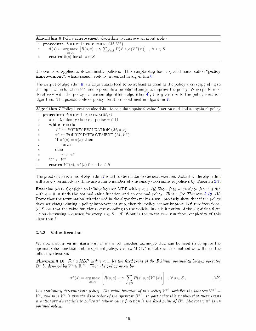
theorem also applies to deterministic policies. This simple step has a special name called �policyimprovement� , whose pseudo-code is presented in algorithm 6.

The output of algorithm 6 is always guaranteed to be at least as good as the policy π corresponding tothe input value function V π, and represents a �greedy� attempt to improve the policy. When performediteratively with the policy evaluation algorithm (algorithm 4), this gives rise to the policy iterationalgorithm. The pseudo-code of policy iteration is outlined in algorithm 7.

Algorithm 7 Policy iteration algorithm to calculate optimal value function and �nd an optimal policy

1: procedure Policy Iteration(M, ε)2: π ← Randomly choose a policy π ∈ Π3: while true do4: V π ← POLICY EVALUATION (M,π, ε)5: π∗ ← POLICY IMPROVEMENT (M,V π)6: if π∗(s) = π(s) then7: break8: else9: π ← π∗

10: V ∗ ← V π

11: return V ∗(s), π∗(s) for all s ∈ S

The proof of correctness of algorithm 7 is left to the reader as the next exercise. Note that the algorithmwill always terminate as there are a �nite number of stationary deterministic policies by Theorem 3.7.

Exercise 3.21. Consider an in�nite horizon MDP with γ < 1. (a) Show that when algorithm 7 is runwith ε = 0, it �nds the optimal value function and an optimal policy. Hint : See Theorem 3.10. (b)Prove that the termination criteria used in the algorithm makes sense: precisely show that if the policydoes not change during a policy improvement step, then the policy cannot improve in future iterations.(c) Show that the value functions corresponding to the policies in each iteration of the algorithm forma non-decreasing sequence for every s ∈ S. (d) What is the worst case run-time complexity of thisalgorithm ?

3.6.3 Value iteration

We now discuss value iteration which is yet another technique that can be used to compute theoptimal value function and an optimal policy, given a MDP. To motivate this method we will need thefollowing theorem:

Theorem 3.10. For a MDP with γ < 1, let the �xed point of the Bellman optimality backup operatorB∗ be denoted by V ∗ ∈ R|S|. Then the policy given by

π∗(s) = arg maxa∈A

[R(s, a) + γ

∑s′∈S

P (s′|s, a)V ∗(s′)

], ∀ s ∈ S , (47)

is a stationary deterministic policy. The value function of this policy V π∗satis�es the identity V π

∗=

V ∗, and thus V ∗ is also the �xed point of the operator Bπ∗. In particular this implies that there exists

a stationary deterministic policy π∗ whose value function is the �xed point of B∗. Moreover, π∗ is anoptimal policy.

19

Proof. We start by noting that π∗ as de�ned in (47) is a stationary deterministic policy, and so we canconclude using (27) that Rπ

∗(s) = R(s, π∗(s)) and Pπ

∗(s′|s) = P (s′|s, π∗(s)) for all s ∈ S and a ∈ A.

As V ∗ is the �xed point of B∗, we have B∗V ∗ = V ∗. So using de�nition (31) of B∗, and (47) we canwrite

V ∗(s) = maxa∈A

[R(s, a) + γ

∑s′∈S

P (s′|s, a)V ∗(s′)

]= R(s, π∗(s)) + γ

∑s′∈S

P (s′|s, π∗(s))V ∗(s′)

= Rπ∗(s) + γ

∑s′∈S

Pπ∗(s′|s)V ∗(s′)

= V π∗(s)

(48)

for all s ∈ S, completing the proof of the �rst part of the theorem.

To prove that π∗ is an optimal policy, we show that if an optimal policy exists then its value functionmust be a �xed point of the operator B∗. So assume that an optimal policy exists, which by Theorem3.8 we can take to be a stationary deterministic policy, and let us denote it as µ and the correspondingoptimal value function as V µ. Now for the sake of contradiction, suppose V µ is not a �xed point ofB∗. Then there exists s ∈ S such that V µ(s) 6= (B∗V µ)(s), which upon combining with Theorem 3.8implies that V µ(s) > (B∗V µ)(s). Then application of Corollary 3.8.1 implies that there exists a policyπ̂ which is strictly better than µ, and so we have a contradiction. This proves that V µ must be theunique �xed point of B∗. Combining this fact with the �rst part implies that V ∗ must be the optimalvalue function and π∗ is an optimal policy. This completes the proof.

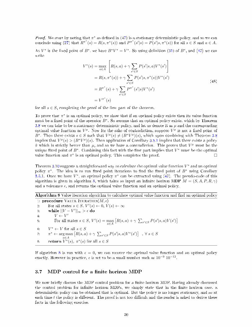
Theorem 3.10 suggests a straightforward way to calculate the optimal value function V ∗ and an optimalpolicy π∗. The idea is to run �xed point iterations to �nd the �xed point of B∗ using Corollary3.5.1. Once we have V ∗, an optimal policy π∗ can be extracted using (47). The pseudo-code of thisalgorithm is given in algorithm 8, which takes as input an in�nite horizon MDP M = (S,A, P,R, γ)and a tolerance ε, and returns the optimal value function and an optimal policy.

Algorithm 8 Value iteration algorithm to calculate optimal value function and �nd an optimal policy

1: procedure Value Iteration(M, ε)2: For all states s ∈ S, V ′(s)← 0, V (s)←∞3: while ||V − V ′||∞ > ε do4: V ← V ′

5: For all states s ∈ S, V ′(s) = maxa∈A

[R(s, a) + γ

∑s′∈S P (s′|s, a)V (s′)

]6: V ∗ ← V for all s ∈ S7: π∗ ← arg max

a∈A

[R(s, a) + γ

∑s′∈S P (s′|s, a)V ∗(s′)

], ∀ s ∈ S

8: return V ∗(s), π∗(s) for all s ∈ S

If algorithm 8 is run with ε = 0, we can recover the optimal value function and an optimal policyexactly. However in practice, ε is set to be a small number such as 10−9-10−12.

3.7 MDP control for a �nite horizon MDP

We now brie�y discuss the MDP control problem for a �nite horizon MDP. Having already discussedthe control problem for in�nite horizon MDPs, we simply state that in the �nite horizon case, adeterministic policy can be obtained that is optimal. But the policy is no longer stationary, and so ateach time t the policy is di�erent. The proof is not too di�cult and the reader is asked to derive thesefacts in the following exercise.

20

Exercise 3.22. Consider a MDP with �nite horizon H and �nite rewards. A typical episode ofthe MDP will look like (s0, a0, s1, a1, . . . , sH−1, aH−1, sH). Let a policy for the MDP be denoted byπ = (π0, π1, . . . , πH−1). Then prove the following statements:

(a) Show that the number of deterministic policies for the MDP is given by H|A||S|.

(b) Assuming that an optimal policy π∗ exists, derive a recurrence relation for the optimal valuefunction V π∗

= (V π∗

0 , . . . , V π∗

H ), with V π∗

H (s) = 0 for all states s ∈ S. Precisely, derive a relationshipbetween V π∗

t and V π∗

t+1.

(c) Let Π be the set of all deterministic policies, i.e. for every π ∈ Π, πt is a deterministic pol-icy at time t and for all times t = 0, . . . ,H − 1. Show that for every policy, deterministic or stochastic,there exists a π ∈ Π which is no worse.

(b) Show that Π contains a policy that is optimal.

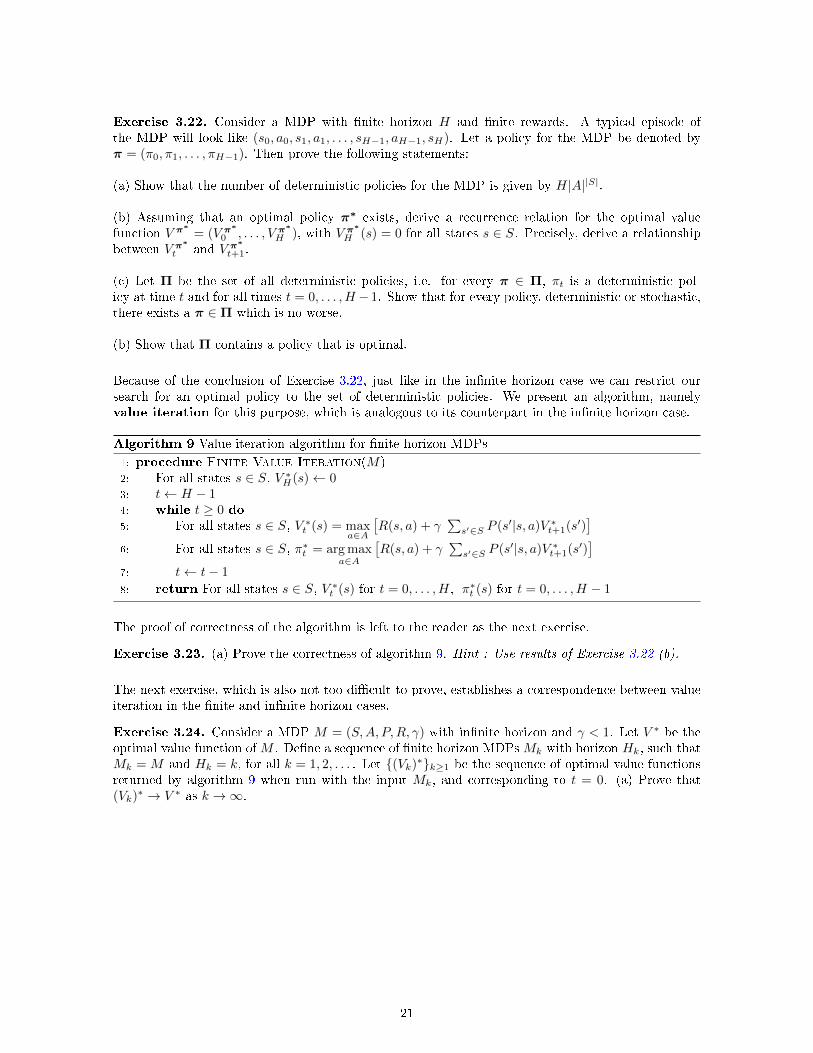
Because of the conclusion of Exercise 3.22, just like in the in�nite horizon case we can restrict oursearch for an optimal policy to the set of deterministic policies. We present an algorithm, namelyvalue iteration for this purpose, which is analogous to its counterpart in the in�nite horizon case.

Algorithm 9 Value iteration algorithm for �nite horizon MDPs

1: procedure Finite Value Iteration(M)2: For all states s ∈ S, V ∗H(s)← 03: t← H − 14: while t ≥ 0 do5: For all states s ∈ S, V ∗t (s) = max

a∈A

[R(s, a) + γ

∑s′∈S P (s′|s, a)V ∗t+1(s′)

]6: For all states s ∈ S, π∗t = arg max

a∈A

[R(s, a) + γ

∑s′∈S P (s′|s, a)V ∗t+1(s′)

]7: t← t− 1

8: return For all states s ∈ S, V ∗t (s) for t = 0, . . . ,H, π∗t (s) for t = 0, . . . ,H − 1

The proof of correctness of the algorithm is left to the reader as the next exercise.

Exercise 3.23. (a) Prove the correctness of algorithm 9. Hint : Use results of Exercise 3.22 (b).

The next exercise, which is also not too di�cult to prove, establishes a correspondence between valueiteration in the �nite and in�nite horizon cases.

Exercise 3.24. Consider a MDP M = (S,A, P,R, γ) with in�nite horizon and γ < 1. Let V ∗ be theoptimal value function ofM . De�ne a sequence of �nite horizon MDPsMk with horizon Hk, such thatMk = M and Hk = k, for all k = 1, 2, . . . . Let {(Vk)∗}k≥1 be the sequence of optimal value functionsreturned by algorithm 9 when run with the input Mk, and corresponding to t = 0. (a) Prove that(Vk)∗ → V ∗ as k →∞.

21

Appendices

A Contraction mapping theorem 1

In this section, we introduce the notion of contraction maps in a Banach space setting, that we haveheavily relied on in the previous section to prove many of our important theorems. The notation usedin this section will be completely independent of what was introduced before, and so the reader shouldread this section in a self-contained fashion.

Let (V, || · ||) be a Banach space, where V is a vector space and || · || is the norm de�ned on the vectorspace. V may be �nite or in�nite dimensional. As it is a Banach space, we remind the reader that thespace is complete, meaning that all Cauchy sequences (De�nition A.1) converge (De�nition A.2). We�rst give a few de�nitions:

De�nition A.1. A sequence {vk}k≥1 of elements vk ∈ V, ∀ k = 1, 2, . . . , is called a Cauchy sequencei� for every real number ε > 0 there exists an integer N ≥ 1, such that ||vm−vn|| < ε for all m,n > N .

De�nition A.2. Let {vk}k≥1 be a sequence of elements of V . We say that the sequence converges toan element v ∈ V , i� for every real number ε > 0 there exists an integer N ≥ 1, such that ||vk−v|| < εfor all k ≥ N . We write this as vk → v.

Our �rst theorem of this section shows that any sequence that is eventually constant is Cauchy.

Theorem A.1. A sequence {vk}k≥1 in a normed vector space that is eventually constant is Cauchy.

Proof. As the sequence is eventually constant, there exists a positive integer r and v ∈ V such that forall k ≥ r, vk = v. Then for any ε > 0, one can choose N = r in De�nition A.1, giving 0 = ||vm−vn|| < εfor all m,n > N , thus completing the proof.

We can now prove that the limit of a Cauchy sequence is unique.

Theorem A.2. A Cauchy sequence {vk}k≥1 in a Banach space converges to a unique limit.

Proof. The fact that the Cauchy sequence converges to a limit is true by the de�nition of a Banachspace. We need to show that this limit is unique. We prove it by contradiction.

Suppose ∃v, w ∈ V, v 6= w, such that vk → v and vk → w. Let δ = ||v − w||, and note that δ > 0 asv 6= w. By De�nition A.2, there exist positive integers M,N such that ||vm − v|| < δ/2 ,∀ m ≥ Mand ||vn − w|| < δ/2 ,∀ n ≥ N . Let l = max(M,N). Then by triangle inequality we have,||v − w|| ≤ ||v − vl||+ ||vl − w|| < δ, which is a contradiction.

We next de�ne the notion of a �contraction map� on a Banach space, and the notion of a ��xed point�of an operator that maps V to itself.

De�nition A.3. A function T : V → V is called a contraction on V i� for every v, w ∈ V , ||Tv−Tw|| ≤||v −w||. The map is called a strict contraction i� there exists a real number 0 ≤ γ < 1, such that forevery v, w ∈ V , ||Tv − Tw|| ≤ γ||v − w||. The constant γ is called the contraction factor of T .

De�nition A.4. Consider a function T : V → V . We say that v ∈ V is a �xed point of T in V , i�Tv = v.

1Additional material that was not covered in class.

22

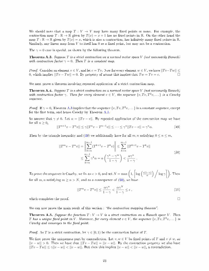
We should note that a map T : V → V may have many �xed points or none. For example, thecontraction map T : R → R given by T (x) = x + 1 has no �xed points in R. On the other hand themap T : R→ R given by T (x) = x, which is also a contraction, has in�nitely many �xed points in R.Similarly, any linear map from V to itself has 0 as a �xed point, but may not be a contraction.

The γ = 0 case is special, as shown by the following theorem.

Theorem A.3. Suppose T is a strict contraction on a normed vector space V (not necessarily Banach)with contraction factor γ = 0. Then T is a constant map.

Proof. Consider an element v ∈ V , and let c = Tv. Now for every element w ∈ V , we have ||Tv−Tw|| ≤0, which implies ||Tv − Tw|| = 0. By property of norms this implies that Tw = Tv = c.

We next prove a theorem involving repeated application of a strict contraction map.

Theorem A.4. Suppose T is a strict contraction on a normed vector space V (not necessarily Banach)with contraction factor γ. Then for every element v ∈ V , the sequence {v, Tv, T 2v, . . . } is a Cauchysequence.

Proof. If γ = 0, Theorem A.3 implies that the sequence {v, Tv, T 2v, . . . } is a constant sequence, exceptfor the �rst term, and hence Cauchy by Theorem A.1.

So assume that γ 6= 0. Let α = ||Tv − v||. By repeated application of the contraction map we havefor all n ≥ 0,

||Tn+1v − Tnv|| ≤ γ||Tnv − Tn−1v|| ≤ · · · ≤ γn||Tv − v|| = γnα. (49)

Then by the triangle inequality and (49) we additionally have for all m,n satisfying 0 ≤ n ≤ m,

||Tmv − Tnv|| =

∥∥∥∥∥m−1∑k=n

(T k+1v − T kv)

∥∥∥∥∥ ≤m−1∑k=n

||T k+1v − T kv||

≤m−1∑k=n

γkα = α

(γn − γm

1− γ

)<

αγn

1− γ.

(50)

To prove the sequence is Cauchy, we �x an ε > 0, and set N = max

(1,

⌈log(ε(1−γ)α

)/log γ

⌉). Then

for all m,n satisfying m ≥ n > N , and as a consequence of (50), we have

||Tmv − Tnv|| ≤ αγn

1− γ<

αγN

1− γ≤ ε , (51)

which completes the proof.

We can now prove the main result of this section : �the contraction mapping theorem�.

Theorem A.5. Suppose the function T : V → V is a strict contraction on a Banach space V . ThenT has a unique �xed point in V . Moreover, for every element v ∈ V , the sequence {v, Tv, T 2v, . . . } isCauchy and converges to the �xed point.

Proof. As T is a strict contraction, let γ ∈ [0, 1) be the contraction factor of T .

We �rst prove the uniqueness part by contradiction. Let v, w ∈ V be �xed points of T and v 6= w, so||v − w|| > 0. Then we have that ||Tv − Tw|| = ||v − w||. By the contraction property we also have||Tv − Tw|| ≤ γ||v − w|| < ||v − w||. But then this implies ||v − w|| < ||v − w||, a contradiction.

23

We now prove the existence part. Take any element v ∈ V and consider the sequence {vk}k≥1 de�nedas follows:

vk =

{v if k = 1,

T vk−1 if k > 1. (52)

Then by Theorem A.4, {vk}k≥1 is a Cauchy sequence, and hence as V is a Banach space, the sequenceconverges to a unique limit v∗ ∈ V by Theorem A.2. We claim that v∗ is a �xed point of T . To provethis, choose any ε > 0 and de�ne δ = ε/(1 + γ). As vk → v∗, by De�nition A.2, ∃ N ≥ 1 such that||vk − v∗|| < δ , ∀ k ≥ N . Then by triangle inequality we have:

||Tv∗ − v∗|| ≤ ||Tv∗ − vN+1||+ ||vN+1 − v∗||= ||Tv∗ − TvN ||+ ||vN+1 − v∗||≤ γ||v∗ − vN ||+ ||vN+1 − v∗||< γδ + δ = ε .

(53)

Thus we have proved that ||Tv∗ − v∗|| < ε for all ε > 0, which implies that ||Tv∗ − v∗|| = 0. As V is anormed vector space, this �nally implies that Tv∗ = v∗, thus completing the existence proof and alsoproving the second part of the theorem.

B Solutions to selected exercises

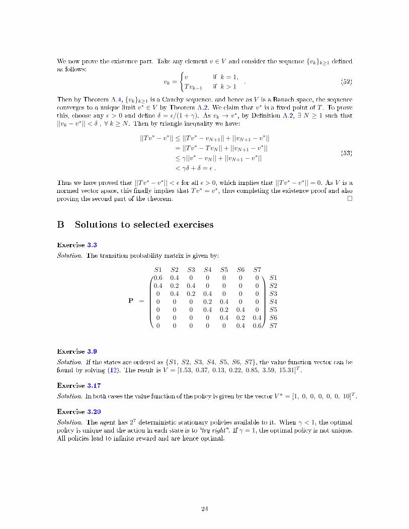
Exercise 3.3

Solution. The transition probability matrix is given by:

P =

S1 S2 S3 S4 S5 S6 S7

0.6 0.4 0 0 0 0 0 S10.4 0.2 0.4 0 0 0 0 S20 0.4 0.2 0.4 0 0 0 S30 0 0 0.2 0.4 0 0 S40 0 0 0.4 0.2 0.4 0 S50 0 0 0 0.4 0.2 0.4 S60 0 0 0 0 0.4 0.6 S7

Exercise 3.9

Solution. If the states are ordered as {S1, S2, S3, S4, S5, S6, S7}, the value function vector can befound by solving (12). The result is V = [1.53, 0.37, 0.13, 0.22, 0.85, 3.59, 15.31]T .

Exercise 3.17

Solution. In both cases the value function of the policy is given by the vector V π = [1, 0, 0, 0, 0, 0, 10]T .

Exercise 3.20

Solution. The agent has 27 deterministic stationary policies available to it. When γ < 1, the optimalpolicy is unique and the action in each state is to �try right�. If γ = 1, the optimal policy is not unique.All policies lead to in�nite reward and are hence optimal.

24