CS 478 - Instance Based Learning1 Instance Based Learning Classify based on local similarity Ranges from simple nearest neighbor to case-based and analogical

CS 478 - Instance Based Learning 1

Instance Based Learning

Classify based on local similarity Ranges from simple nearest neighbor to case-based and

analogical reasoning Use local information near the current query instance to

decide the classification of that instance As such can represent quite complex decision surfaces in a

simple manner– Local model vs a model such as an MLP which uses a global

decision surface

k-Nearest Neighbor Approach Simply store all (or some representative subset) of the

examples in the training set When desiring to generalize on a new instance,

measure the distance from the new instance to one or more stored instances which vote to decide the class of the new instance

No need to pre-process a specific hypothesis (Lazy vs. Eager learning)– Fast learning– Can be slow during execution and require significant storage– Some models index the data or reduce the instances stored to

enhance efficiency

3

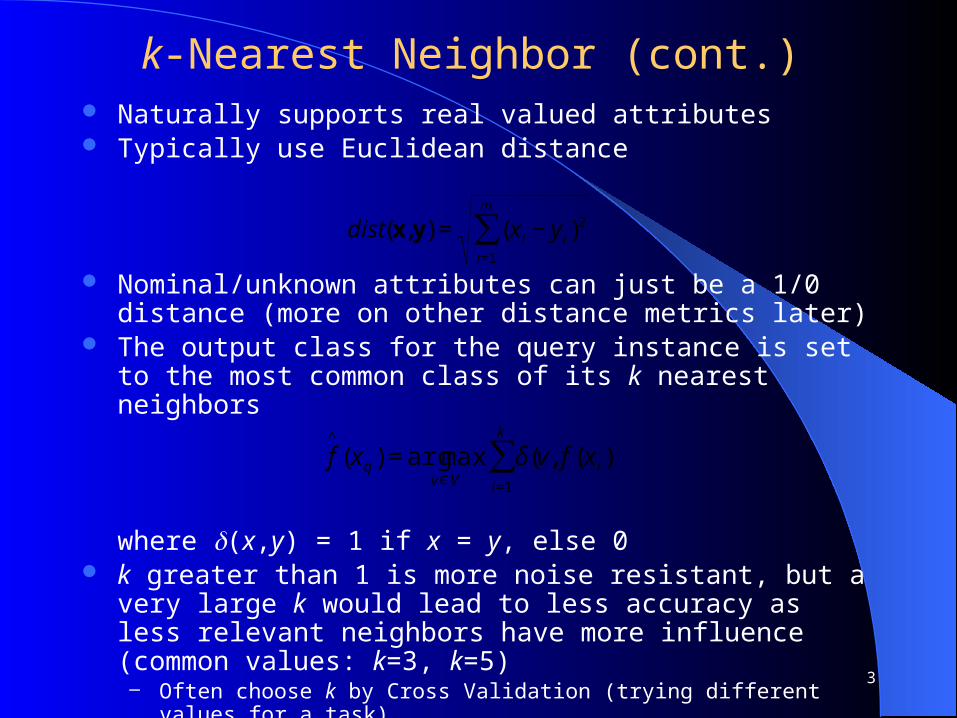
k-Nearest Neighbor (cont.) Naturally supports real valued attributes Typically use Euclidean distance

Nominal/unknown attributes can just be a 1/0 distance (more on other distance metrics later)

The output class for the query instance is set to the most common class of its k nearest neighbors

where (x,y) = 1 if x = y, else 0 k greater than 1 is more noise resistant, but a very large k would lead

to less accuracy as less relevant neighbors have more influence (common values: k=3, k=5)– Often choose k by Cross Validation (trying different values for a task)

€

dist(x,y) = (x i − y i)2

i=1

m

∑

€

f^

(xq ) = argmaxv∈V

δ(v, f (x i))i=1

k

∑

Decision Surface Linear decision boundary between 2 points Combining all the appropriate intersections gives a

Voronoi diagram


Decision Surface Linear decision boundary between 2 points Combining all the appropriate intersections gives a

Voronoi diagram


Euclidean distance – each point a unique class Same points - Manhattan distance


k-Nearest Neighbor (cont.)

Usually do distance weighted voting where the strength of a neighbor's influence is proportional to its distance

Inverse of distance squared is a common weight Gaussian is another common distance weight In this case k value more robust, could let k be even and/or

be larger (even all points if desired), because the more distant points have negligible influence anyway

€

f^

(xq ) = argmaxv∈V

wiδ(v, f (x i))i=1

k

∑

€

wi =1

dist(xq , x i)2


Regression with k-nn Can do non-weighted regression by letting the output be

mean of the k nearest neighbors


Weighted Regression with k-nn

Can also do regression by letting the output be the weighted mean of the k nearest neighbors

For distance weighted regression

Where f(x) is the output value for instance x

€

f^

(xq ) =

wi f (x i)i=1

k

∑

wi

i=1

k

∑

€

wi =1

dist(xq , x i)2

Regression Example

What is the value of the new instance? Assume dist(xq, n8) = 2, dist(xq, n5) = 3, dist(xq, n3) = 4

f(xq) = (8/22 + 5/32 + 3/42)/(1/22 + 1/32 + 1/42) = 2.74/.42 = 6.5 The denominator renormalizes the value


8

5

3

€

f^

(xq ) =

wi f (x i)i=1

k

∑

wi

i=1

k

∑

€

wi =1

dist(xq , x i)2


Attribute Weighting One of the main weaknesses of nearest neighbor is

irrelevant features, since they can dominate the distance– Example: assume 2 relevant and 10 irrelevant features

Can create algorithms which weight the attributes (Note that backprop and ID3 etc. do higher order weighting of features)

Could do attribute weighting - No longer lazy evaluation since you need to come up with a portion of your hypothesis (attribute weights) before generalizing

Still an open area of research– Higher order weighting – 1st order helps, but not enough– Even if just lots of features, all distances become similar, since not

all features are relevant all the time, and the currently irrelevant can dominate distance - need higher-order weighting

– What is the best method, etc.? – important research area


Reduction Techniques Create a subset or other representative set of prototype

nodes– Faster execution, and could even improve accuracy if noisy

instances removed Approaches

– Leave-one-out reduction - Drop instance if it would still be classified correctly - (simplification of CNN)

– Growth algorithm - Only add instance if it is not already classified correctly - both order dependent, similar results – (IB2)

– More global optimizing approaches– Just keep central points – lower accuracy (mostly linear

Voronoi decision surface), best space savings– Just keep border points, best accuracy (pre-process noisy

instances – Drop5)– Drop 5 (Wilson & Martinez) maintains almost full accuracy

with approximately 15% of the original instances Wilson, D. R. and Martinez, T. R., Reduction Techniques for Exemplar-Based Learning Algorithms, Machine Learning Journal, vol. 38, no. 3, pp. 257-286, 2000.


k-Nearest Neighbor Notes

Note that full "Leave one out" CV is easy with k-nn Very powerful yet simple scheme which does well on

many tasks Struggles with irrelevant inputs

– Needs better incorporation of feature weighting schemes

Issues with distance with very high dimensionality tasks– So many features wash out effects of any specifically important

ones (akin to the irrelevant feature problem)– May need distance metrics other than Euclidean distances

Also can be beneficial to reduce total # of instances– Efficiency– Sometimes accuracy



Instance Based Learning Assignment

See http://axon.cs.byu.edu/~martinez/classes/478/Assignments.html

http://axon.cs.byu.edu/~martinez/classes/478/Assignments.html

http://axon.cs.byu.edu/~martinez/classes/478/Assignments.html


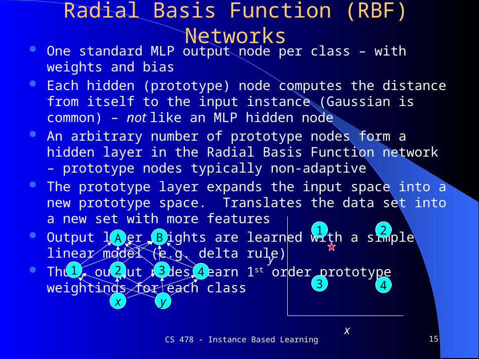
Radial Basis Function (RBF) Networks One standard MLP output node per class – with weights and bias Each hidden (prototype) node computes the distance from itself to the

input instance (Gaussian is common) – not like an MLP hidden node An arbitrary number of prototype nodes form a hidden layer in the Radial

Basis Function network – prototype nodes typically non-adaptive The prototype layer expands the input space into a new prototype space.

Translates the data set into a new set with more features Output layer weights are learned with a simple linear model (e.g. delta

rule) Thus, output nodes learn 1st order prototype weightings for each class

2

A

3

x y

1

B

4

1

x

y

2

3 4


Radial Basis Function Networks

Neural Network variation of nearest neighbor algorithm Output layer execution and weight learning

– Highest node/class net value wins (or can output confidences)– Each node collects weighted votes from prototypes - weighting from

distance (prototype activation – like k-nn), and (unlike k-nn) weighting from learned weights

– Weight learning - Delta rule variations or direct matrix weight calculation – linear or non-linear node activation function

Could use an MLP at the top layer if desired

Key Issue: How many prototype nodes should there be and where should they be placed (means)

Prototype node sphere of influence – Kernel basis function (deviation)– Too small – less generalization, should have some overlap– Too large - saturation, lose local effects, longer training


Node Placement

Random Coverage - Prototypes potentially placed in areas where instances don't occur, Curse of dimensionality

One prototype node for each instance of the training set Random subset of training set instances Clustering - Unsupervised or supervised - k-means style

vs. constructive Genetic Algorithms Node adjustment – Adaptive prototypes (Competitive

Learning style) Dynamic addition and deletion of prototype nodes


RBF vs. BP

Line vs. Sphere - mix-and-match approaches– Multiple spheres still create Voronoi decision surfaces

Potential Faster Training - nearest neighbor localization - Yet more data and hidden nodes typically needed

Local vs Global, less extrapolation (ala BP), have reject capability (avoid false positives)

RBF will have problems with irrelevant features just like nearest neighbor (or any distance based approach which treats all inputs equally)– Could be improved by adding learning into the prototype layer to

learn attribute weighting


Distance Metrics

Wilson, D. R. and Martinez, T. R., Improved Heterogeneous Distance Functions, Journal of Artificial Intelligence Research, vol. 6, no. 1, pp. 1-34, 1997.

Normalization of features Don't know values in novel or data set

instances– Can do some type of imputation and then normal distance

– Or have a distance (between 0-1) for don't know values

Original main question: How best to handle nominal features







Documents

CS 478 - Instance Based Learning1 Instance Based Learning Classify based on local similarity Ranges from simple nearest neighbor to case-based and analogical