1

Crustal and uppermost mantle structure in the central US

encompassing the Midcontinental Rift

Weisen Shen1, Michael H. Ritzwoller1, and Vera Schulte-Pelkum2

1- Department of Physics, University of Colorado at Boulder, Boulder, CO 80309-0390

2 - Cooperative Institute for Research in Environmental Sciences and Department of Geological Sciences, University of Colorado at Boulder, Boulder, CO 80309-0390

Abstract

Rayleigh wave phase velocities across the western arm of the Midcontinent Rift (MCR)

and surrounding regions are mapped by ambient noise eikonal tomography (8-40 sec) and

teleseismic Helmholtz tomography (25 – 80 sec) applied to data from more than 120

Earthscope/USArray stations across the central US. Back-azimuth independent receiver

functions also are computed for those stations using a harmonic stripping technique. A

joint Bayesian Monte-Carlo inversion method is applied to generate 3-D posterior

distributions of shear wave speeds (Vs) in the crust and uppermost mantle to a depth of

about 150 km, providing a synoptic view of the seismic structure of the MCR and its

adjacent tectonic blocks. Three major structural attributes are identified: (1) There is a

high correlation between the long wavelength gravity field and shallow Vs structure,

although the MCR gravity high is obscured by clastic sediments in the shallow crust. (2)

Thick crust (>47 km) underlies the MCR, but structure near the Moho varies along the

rift. (3) Crustal shear wave speeds vary across the Precambrian sutures (e.g., Great Lakes

Tectonic Zone, Spirit Lakes Tectonic Zone). The first observation is consistent with an

upper crustal origin to the MCR gravity anomaly as well as other anomalies in the region.

The thickened crust beneath the MCR is evidence for post-rifting compression with

pure-shear deformation of the crust. The third observation reveals the importance of

Precambrian sutures in the subsequent tectonic evolution of the central US and in

contemporary seismic structure.

2

1. Introduction

The most prominent gravity anomaly in the central US [Woollard and Joesting, 1964] is a

2000-km-long gravity high with two arms merging at Lake Superior and extending

southwest to Kansas and southeast into Michigan. This anomaly has been determined to

mark a late Proterozoic tectonic zone [Whitmeyer and Karlstrom, 2007]. Because of the

existence of mantle-source magmatism and normal faults found along the anomaly, it has

been generally accepted that this anomaly resulted from a continental rifting episode and

as a consequence is known as the Midcontinent Rift system (MCR) [Schmus, 1992] or

Keweenawan Rift system. Geochronological evidence shows that the rift initiated at

about 1.1 Ga and cut through several crustal provinces [Hinze et al., 1997]. Although

various geological and seismic studies have focused on the rift [Hinze et al., 1992;

Mariano and Hinze, 1994; Woelk and Hinze, 1991; Cannon et al., 1989; Vervoort et al.,

2007; Hollings et al., 2010; Hammer et al., 2010; Zartman et al., 2013], the mechanisms

behind the opening and rapid shut down of the rift are still under debate due to lack of

information. Fundamental questions, therefore, remain as to the nature and origin of the

rift system [Stein el al., 2011].

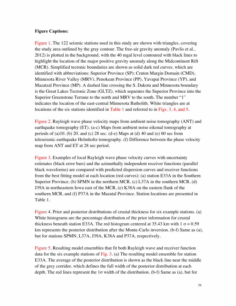
Figure 1 outlines the location of the western arm of the MCR and its neighboring

geological provinces. The MCR can be thought of as being composed of three large-scale

components: the western arm through Minnesota, Iowa, and Kansas; the Lake Superior

arm; and the eastern arm through Michigan. Our focus here is on the western arm. A free

air gravity high defines its location (see 40 mgal anomaly contour in Fig. 1), but divides it

further into three segments: a northern one extending from near the south shore of Lake

Superior along the Wisconsin-Minnesota boundary, a southern one extending from

northeastern to southeastern Iowa, and a small segment in Nebraska and Kansas.

Marginal gravity minima flank the MCR and have been interpreted as a signature of

flanking sedimentary basins [Hinze et al., 1992]. Gravity decreases broadly from 0 - 30

3

mgal in the north to -30 mgal in the south. Whether and how these gravity features relate

to the structure of the crust and uppermost mantle is poorly understood.

The western arm of the MCR remains somewhat more poorly characterized than the Lake

Superior component of the MCR due to a veneer of Phanerozoic sediments [Hinze et al.,

1997]. About two decades ago active seismic studies were performed from northeastern

Wisconsin to northeastern Kansas [Chandler et al., 1989; Woelk and Hinze, 1991] that

revealed a structure similar to the Lake Superior component [Hinze et al. 1992]. These

similarities include crustal thickening to more than 48 km and high-angle thrust faults

that appear to be reactivated from earlier normal faults. Cannon [1994] attributed these

features to a post-rifting compressional episode during the Grenville orogeny.

The MCR cuts across a broad section of geological provinces of much greater age. The

Superior segment of the MCR is embedded in the Archean Superior Province (SP, 2.6-3.6

Ga), which continues into Canada. In Minnesota, this province is subdivided by the Great

Lakes Tectonic Zone (GLTZ) west of the MCR into the 2.6-2.75 Ga Greenstone-Granite

Terrane in the north, and the 3.4-3.6 Ga Gneiss Terrane or “Minnesota River Valley

Sub-Province” (MRV) in the south [Sims and Petermar, 1986]. During the

Paleoproterozoic (1.8-1.9 Ga), the Penokean Province (PP) is believed to have been

accreted to the southern edge of the Superior Province, adding vast foreland basin rocks

and continental rocks along its margin. This is marked as a “craton margin domain

(CMD)” [Holm et al., 2007] in Figure 1. From 1.7-1.8 Ga, the Yavapai province was

added to the southern Minnesota River Valley and the Penokean provinces, which drove

overprinting metamorphism and magmatism along the continental margin to the north.

The East-Central Minnesota Batholith (“1” in Fig. 1) is believed to have been created

during this time [Holm et al., 2007] and this accretion produced the continental suture

known as the Spirit Lake Tectonic Zone (SLTZ). Later (1.65-1.69 Ga), the Mazatzal

Province (MP) was accreted to the Yavapai Province, producing another metamorphic

episode south of the Spirit Lake Tectonic Zone. Overall, the 1.1 Ga rift initiated and

4

terminated in a context provided by geological provinces ranging in age from 1.6 to 3.6

Ga. During the Phanerozoic, this region suffered little tectonic alteration.

In this paper, we aim to produce an improved, uniformly processed 3D image of the crust

and uppermost mantle underlying the western arm of the MCR and surrounding

Precambrian geological provinces and sutures. The purpose is to determine the state of

the lithosphere beneath the region using a unified, well-understood set of observational

methods. We are motivated by a long list of unanswered questions concerning the

structure of the MCR, including the following. (1) How are observed gravity anomalies

related to the crustal and uppermost mantle structure of the region, particularly the

gravity high associated with the MCR? (2) Is the crust thickened (or thinned) beneath the

MCR, and how does it vary along the strike of the feature? (3) Is the MCR structurally a

crustal feature alone or do remnants of its creation and evolution extend into the upper

mantle? (4) Are the structures of the crust and uppermost mantle continuous across

sutures between geological provinces or are they distinct and correlated with such

provinces?

Since 2010, the Earthscope/USArray Transportable Array (TA) left the tectonic western

US and rolled over the region encompassing the western arm of the MCR, making it

possible to obtain new information about the subsurface structure of this feature. The

earlier deployment of USArray stimulated the development of new seismic imaging

methods. This includes ambient noise tomography (e.g., Shapiro et al., 2005; Lin et al.

2008; Ritzwoller et al., 2011) performed with new imaging methods such as eikonal

tomography [Lin et al., 2009] as well as new methods of earthquake tomography such as

Helmholtz tomography [Lin and Ritzwoller, 2011] and related methods [e.g., Pollitz,

2008; Pollitz and Snoke, 2010]. New methods of inference have also been developed

based on Bayesian Monte Carlo joint inversion of surface wave dispersion and receiver

function data (Shen et al., 2013a) that yield refined constraints on crustal structure with

realistic estimates of uncertainties. The application of these methods together have

5

produced a higher-resolution 3-D shear velocity (Vs) model of the western US [Shen et

al., 2013b] with attendant uncertainties and have also been applied on other continents

[e.g., Zhou et al., 2011; Zheng et al., 2011; Yang et al., 2012; Xie et al., 2013]. In this

paper, we utilize more than 120 TA stations that cover the MCR region to produce

high-resolution Rayleigh wave phase velocity maps from 8 to 80 sec period by using

ambient noise eikonal and teleseismic Helmholtz tomography. We then jointly invert

these phase velocity dispersion curves locally with radial component receiver functions to

produce a 3-D Vsv model for the crust and uppermost mantle beneath the western MCR

and the surrounding region.

2. Data Processing

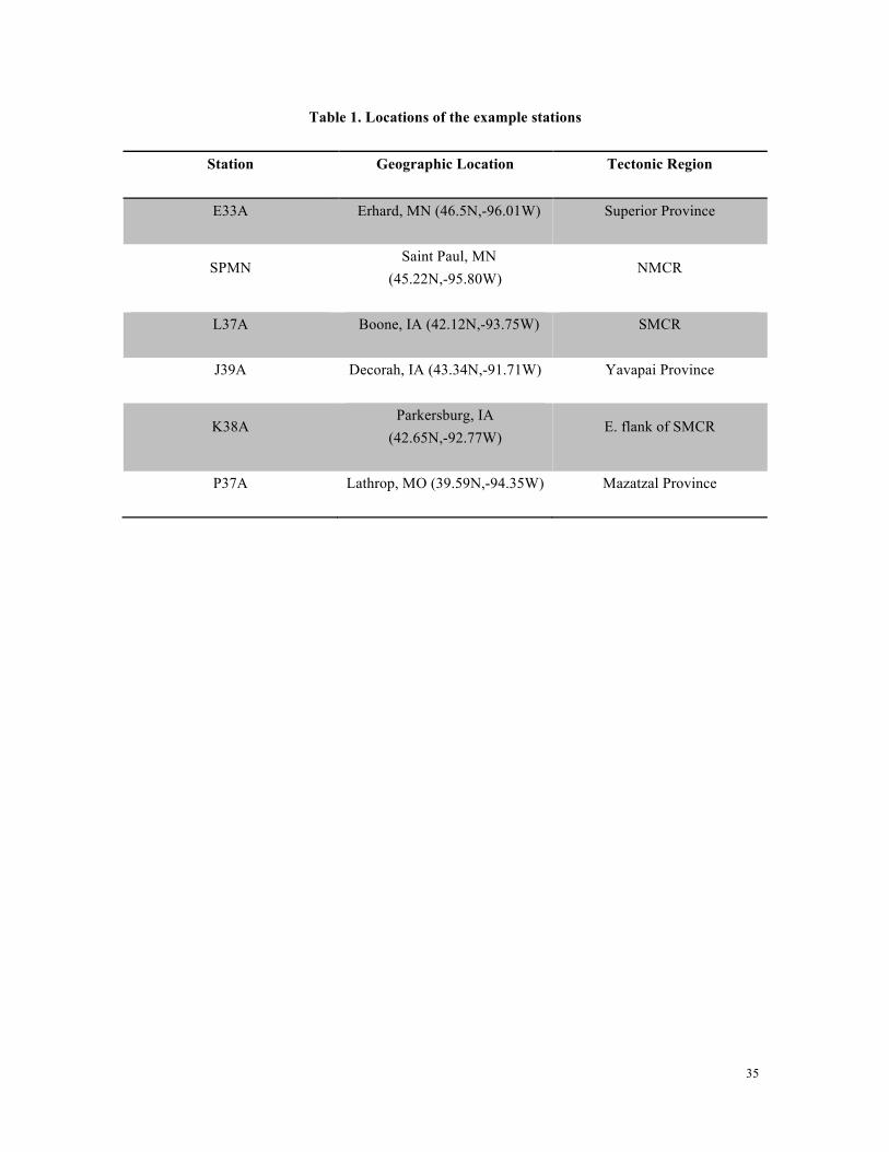
The 122 stations used in this study are shown in Figure 1 as black triangles, which evenly

cover the study area with an average inter-station distance of about 70 km. (Stations at

which we present example results are identified with larger white triangles in Figure 1,

and their names and locations are presented in Table 1.) Based on this station set, we

construct surface wave dispersion curves from ambient noise and earthquake data as well

as receiver functions. Rayleigh wave phase velocity curves from 8 to 80 sec period are

taken from surface wave dispersion maps generated by eikonal tomography based on

ambient noise and Helmholtz tomography based on teleseismic earthquakes. We also

construct a back-azimuth independent receiver function at each station by the harmonic

stripping technique. Details of these methods have been documented in several papers

(eikonal tomography: Lin et. al., 2009; Helmholtz tomography: Lin and Ritzwoller et al.,

2011; harmonic stripping: Shen et al., 2013a) and are only briefly summarized here.

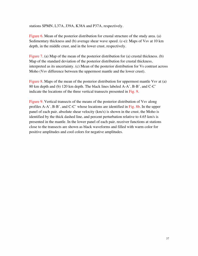
2.1. Rayleigh wave dispersion curves

We measured Rayleigh wave phase velocities from 8 to 40 sec period from the ambient

noise cross-correlations based on the USArray TA stations available from 2010 to May

2012. We combined the 122 stations in the study area with the TA stations to the west of

6

the area [Shen et al. 2013b] in order to increase the path density. The ambient noise data

processing procedures are those described by Bensen et al. [2007] and Lin et al. [2008],

and produce more than 10,000 dispersion curves in the region of study. At short periods

(8 to 40 sec), eikonal tomography [Lin et al., 2009] produces Rayleigh wave phase

velocity maps with uncertainties based on ambient noise (e.g., Fig. 2a-c). For longer

periods (25 to 80 sec), Rayleigh wave phase velocity measurements are obtained from

earthquakes using the Helmholtz tomography method [Lin and Ritzwoller, 2011]. A total

of 875 earthquakes between 2010 and 2012 with Ms > 5.0 are used, and on average each

station records acceptable measurements (based on a SNR criterion) from about 200

earthquakes for surface wave analysis. Example maps are presented in Figure 2d,e. In the

period band of overlap between the ambient noise and earthquake measurements (25 to

40 sec), there is strong agreement between the resulting Rayleigh wave maps (Fig. 2f).

The average difference is ~ 0.001 km/sec, and the standard deviation of the difference is

~ 0.012 km/sec, which is within the uncertainties estimated for this period (~0.015

km/sec).

At 10 sec period, at which Rayleigh waves are primarily sensitive to sedimentary layer

thickness and the uppermost crystalline crust, a slow anomaly is seen in the gap between

the northern and southern MCR, and runs along the flanks of the MCR, particularly in the

south. Wave speeds are high north of the Great Lakes Tectonic Zone (GLTZ) and

average in the Mazatzal Province. Between 20 and 40 sec, the most prominent feature is

the low speed anomaly that runs along the MCR, as was also seen by Pollitz and Mooney

[2013]. This indicates low shear wave speeds in the lower crust/uppermost mantle and/or

a thickened crust beneath the MCR. Higher wave speeds at these periods appear mostly

north of the Great Lakes Tectonic Zone. At longer periods, the anomaly underlying the

MCR breaks into northern and southern parts and the lowest wave speeds shift off the rift

axis near the southern MCR. With these Rayleigh wave phase speed dispersion maps at

periods between 8 and 80 sec, we produce a local dispersion curve at each station

7

location. For example, the local Rayleigh wave phase velocity curve with uncertainties at

station E33A in the southern Superior Province is shown in Figure 3a with black error

bars. Other example Rayleigh wave curves are presented in Figure 3b-f.

2.2 Receiver function processing

The method we use to process receiver functions for each station is described in detail in

Shen et al. [2013b]. For each station, we pick earthquakes from the years 2010, 2011 and

2012 in the distance range from 30° to 90° with mb > 5.0. We apply a time domain

deconvolution method [Ligorria and Ammon, 1999] to each seismogram windowed

between 20 sec before and 30 sec after the P-wave arrival to calculate radial component

receiver functions with a low-pass Gaussian filter with a width of 2.5 s (pulse width ~ 1

sec), and high-quality receiver functions are selected via an automated procedure.

Corrections are made both to the time and amplitude of each receiver function,

normalizing to a reference slowness of 0.06 sec/km [Jones and Phinney, 1998]. Finally,

only the first 10 sec after the direct P arrival is retained for further analysis. We compute

the azimuthally independent receiver function, R0(t), for each station by fitting a

truncated Fourier Series at each time over azimuth and stripping the azimuthally variable

terms using a method called “harmonic stripping” by Shen et al. [2013b]. This method

exploits the azimuthal harmonic behavior in receiver functions (e.g., Girardin and Farra,

1998; Bianchi et al., 2010). After removing the azimuthally variable terms at each time,

the RMS residual over azimuth is taken as the 1σ uncertainty at that time.

On average, about 72 earthquakes satisfy the quality control provisions for each station

across the region of study, which is about half of the average number of similarly high

quality recordings at the stations in the western US [Shen et al., 2013b]. This reduction in

the number of accepted receiver functions results primarily from the distance range for

teleseismic P (30o to 90o), which discards many events from the southwest Pacific (e.g.,

Tonga). The number of retained earthquakes varies across the region of study, being

highest towards the southern and western parts of the study region and lowest towards the

8

north and east. At some stations there are as few as 21 earthquake records retained and

receiver functions at 15 stations display a large gap in back-azimuth, which prohibits

estimating stable, azimuthally-independent receiver functions. For these stations, we use

a simple, directly-stacked receiver function to represent the local average. Overall, the

quality of the resulting azimuthally independent receiver functions is significantly lower

than observed across the western US by Shen et al. [2013a,b] where more than 100

earthquakes are typically retained for receiver function analysis.

Examples of receiver functions at six stations in the MCR region are shown in Figure 3

as parallel black lines that delineate the one standard deviation uncertainty at each time.

At station E33A (Fig. 3a) in the southern Superior Province, a clear Moho conversion

appears at ~ 4.3 sec after the direct P arrival, which indicates a distinct, shallow (~ 35 km)

Moho discontinuity. In contrast, at station SPMN in the northern MCR (Fig. 3b) only a

subtle Moho Ps conversion is apparent, which suggests a gradient Moho beneath the

station. In the southern MCR, the receiver function at station L37A (Fig. 3c) has a strong

Moho Ps signal at ~ 6 sec, implying the Moho discontinuity is at over 45 km depth. At

station J39A to the east of the MCR (Fig. 3d), a Ps conversion at ~4.5 sec is observed,

indicating a much thinner crust. At K38A, which is located in the gravity low of the

eastern flank of the southern MCR (Fig. 3e), a sediment reverberation appears after the P

arrival. In the Mazatzal Province at station P37A (Fig. 3f) a relatively simple receiver

function is observed with a Ps conversion at ~ 5.3 sec, indicative of crust of intermediate

thickness in this region.

3. Construction of the 3-D model from Bayesian Monte Carlo joint inversion

Here we briefly summarize the joint Bayesian Monte Carlo inversion of surface wave

dispersion curves and receiver functions generated in the steps described in section 2. A

1-D joint inversion of the station receiver function and dispersion curve is performed on

the unevenly distributed station grid and then the resulting models from all stations are

interpolated into the 3-D model using a simple kriging method, as described by Shen et al.

9

[2013b].

3.1 Model space and prior information

We currently only measure Rayleigh wave dispersion, which is primarily sensitive to Vsv,

so we assume the model is isotropic: Vsv=Vsh=Vs. The Vs model beneath each station is

divided into three principal layers. The top layer is the sedimentary layer defined by three

unknowns: layer thickness and Vs at the top and bottom of the layer with Vs increasing

linearly with depth. The second layer is the crystalline crust, parameterized with five

unknowns: four cubic B-splines and crustal thickness. Finally, there is the uppermost

mantle layer, which is given by five cubic B-splines, yielding a total of 13 free

parameters at each location. The thickness of the uppermost mantle layer is set so that the

total thickness of all three layers is 200 km. The model space is defined based on

perturbations to a reference model consisting of the 3D model of Shapiro and Ritzwoller

[2002] for mantle Vs, crustal thickness and crustal shear wave speeds from CRUST 2.0

[Bassin et al., 2000], and sedimentary thickness from Mooney and Kaban [2010].

Because the reference sediment model is inaccurate in the region of study, we empirically

reset the reference sedimentary thickness at stations that display strong sedimentary

reverberations in the receiver functions.

The following three prior constraints are introduced in the Monte Carlo sampling of

model space. (1) Vs increases with depth at the two model discontinuities (base of the

sediments and Moho). (2) Vs increases monotonically with depth in the crystalline crust.

(3) Vs < 4.9 km/sec at all depths. These prior constraints reduce the model space

effectively. Following Shen et al. [2013b], the Vp/Vs ratio is set to be 2 for the

sedimentary layer and 1.75 in the crystalline crust/upper mantle (consistent with a

Poisson solid). Density is scaled from Vp by using results from Christensen and Mooney

[1995] and Brocher [2005] in the crust and Karato [1993] in the mantle. The Q model

from PREM [Dziewonski and Anderson, 1981] is used to apply the physical dispersion

correction [Kanamori and Anderson, 1977] and our resulting model is reduced to 1 sec

10

period. Increasing Q in the upper mantle from 180 to 280 will reduce the resulting Vs by

less than 0.5% at 80 km depth.

As described by Shen et al. [2013b], the Bayesian Monte Carlo joint inversion method

constructs a prior distribution of models at each location defined by allowed perturbations

relative to the reference model as well as the model constraints described above.

Examples of prior marginal distributions for crustal thickness at the six example stations

are shown as white histograms in Figure 4. The nearly uniform distribution of the prior

illustrates that we impose weak prior constraints on crustal thickness.

3.2 Joint Monte Carlo inversion and the posterior distribution

Once the data are prepared and the prior model space is determined, we follow Shen et al.

[2013b] and perform a Markov Chain Monte Carlo inversion. At each location, we

consider at least 100,000 trial models in which the search is guided by the Metropolis

algorithm. Models are accepted into the posterior distribution or rejected according to the

square root of the reduced χ2 value. A model m is accepted if χ(m) > χmin + 0.5, where

χmin is the χ value of the best fitting model. After the inversion, the misfit to the Rayleigh

wave dispersion curve has a χmin value less than 1 for all the stations. For receiver

function data, χmin is less than 1 for more than 95% of the stations. At six stations, χmin > 1

for the receiver functions: At two of these stations, multiple arrivals in the receiver

functions cannot be fit with our simple model parameterization and probably require the

introduction of further layers in the crust. The other four stations lie near the boundaries

of our study region where the receiver functions are of lower quality.

The principal output of the joint inversion at each station is the posterior distribution of

models that satisfy the receiver function and surface wave dispersion data within

tolerances that depend on the ability to fit the data and data uncertainties as discussed in

the preceding paragraph. The statistical properties of the posterior distribution quantify

model errors. In particular, the mean and standard deviation (interpreted as model

11

uncertainty) of the accepted model ensemble are computed from the posterior distribution

at each depth within the model.

Figure 4 shows posterior distributions for crustal thickness for the example stations as red

histograms. Compared with the prior distributions (white histograms), the posterior

distributions narrow significantly at five of the six stations, meaning that at these stations

crustal thickness is fairly tightly constrained (σ < 2 km) with a clear Moho Ps conversion

in the receiver function (Fig. 3a). The exception is station SPMN (Fig. 3b) in the northern

MCR where there is a weak Moho Ps conversion (σ > 5 km). In the six examples

presented in Figure 4, crustal thickness ranges from about 35 to 48 km. Over the entire

region of study, crustal thickness has a mean value of 44.8 km and an average 1σ

uncertainty of about 3.3 km.

Inversion results for the six example stations are shown in Figure 5. The clear Moho with

small depth uncertainty at station E33A reflects the strong Moho Ps signal in the

back-azimuth averaged receiver function (Fig. 3a). Both the Rayleigh wave dispersion

and the receiver function are fit well at this station (Fig. 3a). In contrast, at station SPMN

(Fig. 5b) a gradient Moho appears in the model because the receiver function does not

have a clear Ps conversion (Fig. 3b).

The resulting models for the other four stations (L37A, J39A, K38A, P37A) are shown in

Figure 5c-f and the fit to the data is shown in Figure 3c-f. Station L37A is located near

the center of the southern MCR. The receiver functions computed at this station show a

relatively strong Moho Ps conversion at ~ 6 sec after the direct P arrival, indicating a

sharp Moho discontinuity at ~ 50 km depth with uncertainty of about 1.75 km. For station

J39A in northeastern Iowa, the clear Ps conversion at ~ 5 sec indicates a much shallower

Moho discontinuity at ~ 40 km with an uncertainty of about 1 km. For station K38A near

the eastern flank of the southern MCR, strong reverberations in the receiver function

indicate the existence of thick sediments but there is also a clear Moho Ps arrival. Finally,

a clear Moho with uncertainty less than 1 km is seen beneath station P37A in the

12

Mazatzal province.

We perform the joint inversion for all 122 TA stations in the region of study and

construct a mean1-D model with uncertainties for each station. We then interpolate those

1-D models onto a regular 0.25°x 0.25°grid by using a simple kriging method in order

to construct a 3-D model for the study region [Shen et al. 2013a].

Maps of the 3-D model for various model characteristics are shown in Figures 6-8.

Figure 6 presents map views of the 3-D model within the crust: average thickness and Vs

of the sedimentary layer (Fig. 6a,b, respectively), Vs at 10 km depth (Fig. 6c), middle

crust defined as the average in the middle 1/3 of the crystalline crust (Fig. 6d), and lower

crust defined as the average from 80% to 100% of the depth to the Moho (Fig. 6e). Moho

depth, uncertainty in Moho depth, and the Vs contrast across the Moho (the difference

between Vs in uppermost mantle and lower crust) are shown in Figure 7a-c. Deeper

structures in the mantle are presented in Figure 8 with Vs maps at 80 km depth (Fig. 8a)

and 120km (Fig. 8b). Three vertical slices that cross the MCR are shown in Figure 9

along profiles identified as A-A’, B-B’ and C-C’ in Figure 8b. The model is discussed in

more detail in section 4. Although the 3-D model extends to 200 km below the surface of

the earth, the Vs uncertainties increase with depth below 150 km due to the lack of

vertical resolution. Therefore, we only discuss the top 150 km of the 3-D model.

4. Results and Discussion

4.1 Sedimentary layer

The sedimentary layer structure is shown in Figure 6a,b. Thick sediments (> 2 km) are

observed near the eastern flank of the southern MCR, thinning southward. Another thick

sedimentary layer appears near the southern edge of the MCR in Kansas. In the rest of the

area, the sediments are relatively thin (<1 km). However, because the sedimentary

structure is mainly inferred by receiver functions, the resulting sedimentary distribution

may be spatially aliased due to the high lateral resolution of the receiver functions (< 5

13

km) with a low spatial sampling rate at the station locations (~ 70 km). The receiver

functions also indicate the existence of sediments with particularly low shear wave

speeds in some areas. For example, strong reverberations observed in the receiver

function for station E33A in the first 2 sec may be fit by a Vs model with a thin (< 0.5 km)

but slow Vs layer (< 1.8 km/sec) near the surface (Fig. 3a). Figure 6b shows the pattern

of the inferred Vs in the sedimentary layer, which differs from the sedimentary thickness

map. Very slow sedimentary shear wave speeds are found in northern Minnesota, which

may be due to the moraine associated with the Wadena glacial lobe [Wright, 1962]. Some

of the slow sediments generate strong reverberations in the receiver functions that

coincide in time with the Moho signal, resulting in large uncertainties in the crustal

thickness map (Fig. 7b). At some other stations, sedimentary reverbarations do not

obscure the Moho Ps arrival; e.g., K38A (Fig. 3e). Sedimentary reverberations in the

receiver functions can also be seen in Figure 9 beneath the Yavapai Province in transects

B-B’ and C-C’, beneath the southern MCR in transect C-C’, and north of the southern

MCR in transect C-C’.

4.2 Correlations of crustal structure with the observed gravity field

The MCR gravity high (40 mgal anomaly outlined in the free air gravity map of Fig. 1) is

poorly correlated with the shear velocity anomalies presented in Figures 6-8. Because

positive density anomalies should correlate to positive velocity anomalies [Woollard,

1959], the expectation is that high velocity anomalies underlie the MCR or the crust is

thin along the rift. In fact, the opposite is the case. At 10 km depth, low velocity

anomalies run beneath the rift and, on average, the crust is thickened under the rift. Our

3D model does therefore not explain the gravity high that lies along the MCR. There are

two possible explanations for this. First, the high-density bodies that cause the gravity

high may be too small to be resolved with surface wave data determined from the station

spacing presented by the USArray. Second, small high shear wave speed bodies that

cause the gravity high may be obscured by sediments in and adjacent to the rift. We

14

believe the latter is the more likely cause of the anti-correlation between observed gravity

anomalies and uppermost crustal shear velocity structure beneath the rift. If this is true,

however, the high-density bodies that cause the gravity high would have to be in the

shallow crust, else they would imprint longer period maps that are less affected by

sediments. This is consistent with the study of Woelk and Hinze [1991] who argue that

the uppermost crust beneath the MCR contains both fast igneous rocks and slow clastic

rocks. Under this interpretation, shallow igneous rocks must dominate the gravity field

while the clastic rocks dominate the shear wave speeds. A shallow source for the gravity

anomaly is also supported by the observation that the eastern arm of the MCR, which is

buried under the Michigan Basin, has a much weaker gravity signature than the western

arm imaged in this study [Stein et al., 2011].

The 3D shear velocity model is better correlated with the longer wavelengths in the

gravity map (Fig. 1), which displays a broad gradient across the region [von Frese et al.,

1982]. The free-air gravity southeast of the MCR is lower (-30 mgal) than in the

northwestern part of the map (10-20 mgal). It has been argued that this gradient is not due

to variations in Precambrian structure across the sutures [Hinze et al., 1992], but may be

explained by a density difference in an upper crustal layer. Our results support an upper

crustal origin because the correlation of high shear velocities with positive long

wavelength gravity anomalies exists primarily at shallow depths. At 10 km depth, which

is in the uppermost crystalline crust (Fig. 6c), the most prominent shear velocity feature is

a velocity boundary that runs along the western flank of the MCR. This follows the

Minnesota River Valley Province-Yavapai Province boundary in the west and the

northeastern edge of the Craton Margin Domain in the east. North of this boundary, Vs is

between 3.65 and 3.7 km/sec in the southern Superior Province, while to the south it

decreases to between 3.5 and 3.6 km/sec in the Minnesota River Valley, Yavapai

Province and Mazatzal Province. This boundary lies near the contrast in free air gravity.

Similar features do not appear deeper in the model (Figs. 6d,e, 7).

15

Because receiver functions are sensitive to the discontinuity between the sediments and

the crystalline crustal basement, the commonly unresolved trade-off between crustal

structure and deeper structure in traditional surface wave inversions [e.g., Zheng et al.,

2010; Zhou et al., 2011] has been ameliorated in the model we present here.

Consequently, we believe that the Vs heterogeneity present at 10 km depth in the model

does not arise from a vertical smearing effect in the inversion, that the high correlation of

Vs with the long-wavelength gravity field is confined to the upper crust, and that the

source of the long wavelength gravity trend is in the upper crust.

Additionally, there are correlations between shallow Vs structure and short wavelength

gravity anomalies. (1) In the gravity map, the lowest amplitudes appear near station

K34A on the eastern flank of the southern MCR where thick sediments are present in the

model (Fig. 5e). Thus, local gravity minima may be due to the presence of local

sediments. (2) At 10km, a very slow anomaly (< 3.5 km/sec) is observed in the gap

between the northern and southern MCR, which implies an upper crustal depth for the

discontinuity in the MCR in this area. It is not clear why such low shear wave speeds

appear in the upper crust here.

4.3 Relationship between Precambrian sutures and observed crustal structures

4.3.1 Great Lakes Tectonic Zone

In the northern part of the study region, the Great Lakes Tectonic Zone (GLTZ) suture

that lies between the 2.7 -2.75 Ga greenstone terrane to the north and the 3.6 Ga

granulite-facies granitic and mafic gneisses Minnesota River Valley sub-province to the

south cuts the southern end of Superior Province into two sub-provinces [Morey and

Sims, 1976]. The eastern part of Great Lakes Tectonic Zone in our study region is

covered by the Craton Margin Domain (CMD of Fig. 1), which contains several

structural discontinuities [Holm et al., 2007].

Beneath this northernmost suture, a Vs contrast is observed in the 3-D model through the

16

entire crust, increasing with depth. In the upper crust (Fig. 6c), Vs is ~ 3.7 km/sec

beneath the Superior Province (SP) greenstone terrane and ~ 3.68 km/sec beneath the

Minnesota River Valley (MRV) with a relatively slow Vs belt beneath the eastern part of

the suture. In the middle crust (Fig. 6d), the Vs contrast is stronger. A fast anomaly (> 3.8

km/sec) is observed beneath the MRV itself, perhaps indicating a more mafic middle

crust, while in the north the SP is about 0.08 km/sec slower than the MRV. This

difference across the Great Lakes Tectonic Zone grows with depth to about 0.15 km/sec

in the lowermost crust (Fig. 6e).

These variations in crustal structure are also reflected in Moho depth, which is discussed

further in section 4.4. North of the GLTZ, a clear, large-amplitude Moho signal is seen as

early as 4.3 sec (Fig. 3a), although the receiver functions at some stations display large

reverberations from the thin slow sediments. Combined with relatively fast phase

velocities observed at 28 sec period in this area, the inversion yields a relatively shallow

Moho at about 36 km depth at station E33A and its neighboring points. To the south of

the GLTZ, thicker crust is found in the MRV with an average crustal thickness of about

46 km with a maximum thickness of about 48 km. The average uncertainties of crustal

thickness in the MRV are greater than 3 km suggesting that the Moho is more of a

gradient than a sharp boundary (Fig. 7c). A seismic reflection study in this area (Boyd

and Smithson, 1994) reveals localized Moho layering probably due to mafic intrusions

related to post-Archean crustal thickening events in this area. Our large Moho depth and

fast middle to lower crust (Fig. 6d,e) are consistent with this interpretation.

4.3.2 Spirit Lakes Tectonic Zone

The boundary between the Superior (SP) and the Yavapai (YP) provinces is the Spirit

Lakes Tectonic Zone (SLTZ), which extends east through the middle of the MCR into

Wisconsin. East of the MCR, the SLTZ separates the Penokean Province to the north

from the Yavapai Province to the south. As described in section 4.2, west of the MCR

this suture forms a boundary within the upper crystalline crust that correlates with the

17

gravity map. Structural differences between the two provinces across the suture continue

into the lower crust, with faster Vs in the Minnesota River Valley subprovince and slower

Vs in the Yavapai. In terms of Moho topography, the Yavapai Province has relatively

thinner crust (~ 44-45 km), becoming thinner east of the southern MCR (~ 39 km). In

particular, the receiver function at station J39A (Fig. 3d) displays a clear Moho Ps

conversion at about 4.5 sec after the direct P arrival. The resulting model for station J39A

is shown in Figure 4d with a crustal thickness of about 38±1.5km. This is the thinnest

crust in the vicinity of the rift, but is still deeper than in the Greenstone terrane in the

western part of the Superior Province.

4.3.3 Boundary between the Yavapai and Mazatzal provinces

The third and southernmost suture in the study region is the boundary between the

Yavapai (YP) and Mazatzal provinces (MP) near the Iowa-Missouri border, extending in

the NE-SW direction. Compared with the structural variations across the more northerly

sutures, the variations across this suture are subtler both in crustal velocities and crustal

thickness. However, lower crustal Vs is slower (< 4 km/sec) in the YP than it in the MP

(> 4 km/sec).

In summary, the three major Precambrian sutures in the region are associated with crustal

seismic structural variations, especially across the northern (GLTZ) and middle (SLTZ)

sutures in the MCR region. Later cumulative metamorphism of early Proterozoic

accretionary tectonics [Holm et al., 2007] may have obscured structural variations across

the Yavapai – Mazatzal boundary.

4.4 Variations in crustal thickness

An advantage of the joint inversion of surface wave dispersion and receiver functions is

the amelioration of trade-offs that occur near structural discontinuities such as the base of

the sediments and the Moho, which hamper inversion of surface wave data alone. As

argued by Shen et al. [2013a,b] and many others [Bodin et al., 2012; Lebedev et al.,

18

2013], estimates of depth to Moho as well as the velocity contrast across it are greatly

improved and we believe that our estimates of crustal thickness beneath the MCR are

reliable.

The map of estimated Moho topography (Fig. 7a) shows that the MCR has a deep Moho

(>47 km, peaking at ~50 km) in all three segments (Wisconsin/Minnesota, Iowa,

Nebraska/Kansas). The crust beneath the MCR is about 5 km thicker, on average, than

crustal thickness averaged across the study region. For the northern MCR, the crustal

thickening mostly occurs within the gravity anomaly and extends to the northeastern edge

of the Craton Margin Domain. In the southern MCR, crustal thickening is not uniform

along the rift but is most pronounced in the southern half of this segment. For the

Nebraska/Kansas segment, thickened crust (> 47 km) is also present, which is consistent

with a previous reflection study for this area [Woelk and Hinze, 1991].

Uncertainties in crustal thickness for the northern segment of the MCR are larger (> 4km)

than for the southern segment (<2 km), as Figure 7b shows. This is because receiver

functions in the south display a clear P-to-S conversion associated with Moho and the

Moho has a larger velocity jump across it (Fig. 5c), about 0.4 km/s in the northern

segment and 0.55 – 0.7 km/s in the south. Between the northern and southern segments,

there is a shallow Moho (< 42 km) that extends eastward to the eastern Penokean Orogen

and perhaps further east.

Notable crustal thickness variations are observed in the rest of the study area as well: a

significantly thinned crust is seen near the western border of Minnesota within the

Superior Province, which changes to a thick crust with a gradient Moho at about 50 km

depth in the Gneiss Terrane of the Minnesota River Valley to the south. Another gradient

Moho is observed north of the Great Lakes Tectonic Zone in the Superior Province,

which is consistent with a previous reflection seismic survey in the area [Boyd and

Smithson, 1994]. Further south, crustal thickness lies between 42 km and 46 km in the

Mazatzal Province.

19

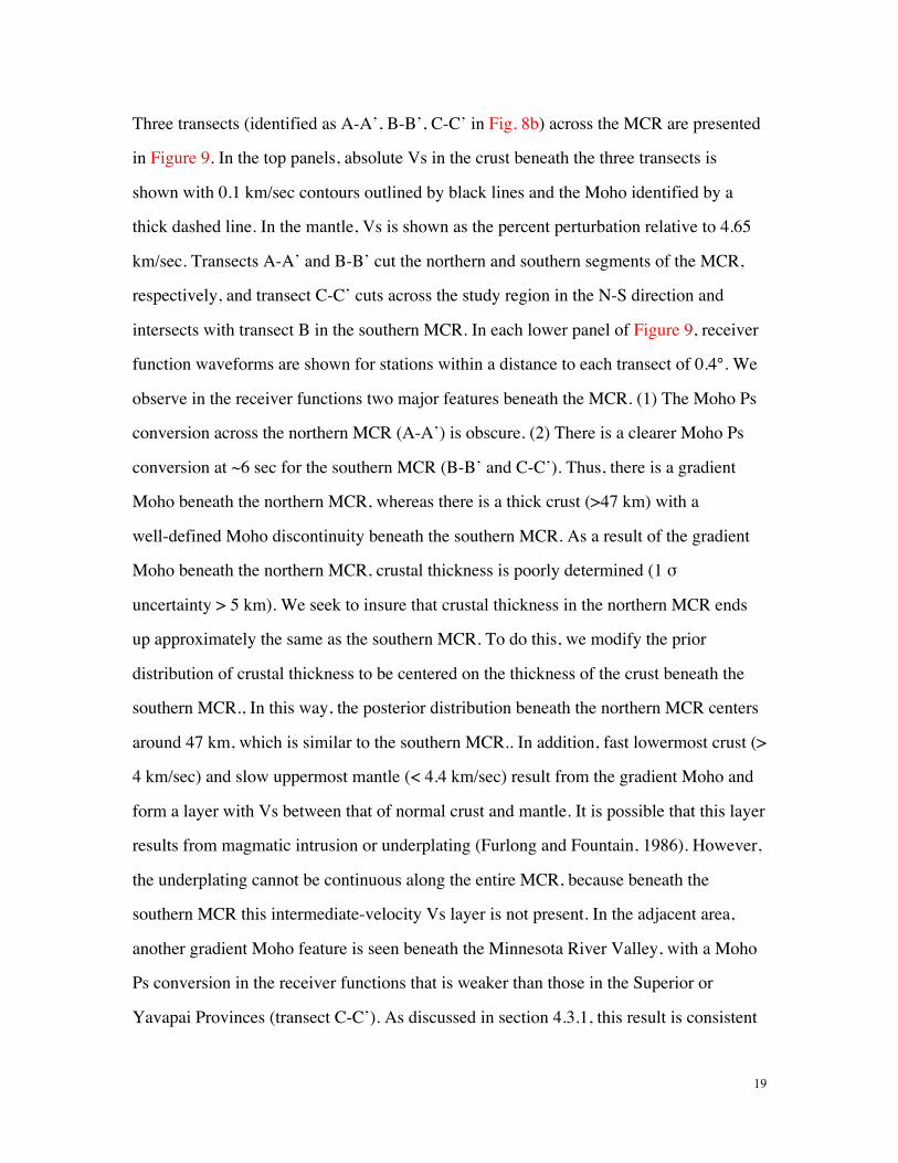
Three transects (identified as A-A’, B-B’, C-C’ in Fig. 8b) across the MCR are presented

in Figure 9. In the top panels, absolute Vs in the crust beneath the three transects is

shown with 0.1 km/sec contours outlined by black lines and the Moho identified by a

thick dashed line. In the mantle, Vs is shown as the percent perturbation relative to 4.65

km/sec. Transects A-A’ and B-B’ cut the northern and southern segments of the MCR,

respectively, and transect C-C’ cuts across the study region in the N-S direction and

intersects with transect B in the southern MCR. In each lower panel of Figure 9, receiver

function waveforms are shown for stations within a distance to each transect of 0.4°. We

observe in the receiver functions two major features beneath the MCR. (1) The Moho Ps

conversion across the northern MCR (A-A’) is obscure. (2) There is a clearer Moho Ps

conversion at ~6 sec for the southern MCR (B-B’ and C-C’). Thus, there is a gradient

Moho beneath the northern MCR, whereas there is a thick crust (>47 km) with a

well-defined Moho discontinuity beneath the southern MCR. As a result of the gradient

Moho beneath the northern MCR, crustal thickness is poorly determined (1 σ

uncertainty > 5 km). We seek to insure that crustal thickness in the northern MCR ends

up approximately the same as the southern MCR. To do this, we modify the prior

distribution of crustal thickness to be centered on the thickness of the crust beneath the

southern MCR., In this way, the posterior distribution beneath the northern MCR centers

around 47 km, which is similar to the southern MCR.. In addition, fast lowermost crust (>

4 km/sec) and slow uppermost mantle (< 4.4 km/sec) result from the gradient Moho and

form a layer with Vs between that of normal crust and mantle. It is possible that this layer

results from magmatic intrusion or underplating (Furlong and Fountain, 1986). However,

the underplating cannot be continuous along the entire MCR, because beneath the

southern MCR this intermediate-velocity Vs layer is not present. In the adjacent area,

another gradient Moho feature is seen beneath the Minnesota River Valley, with a Moho

Ps conversion in the receiver functions that is weaker than those in the Superior or

Yavapai Provinces (transect C-C’). As discussed in section 4.3.1, this result is consistent

20

with a seismic reflection study in this sub-province [Boyd and Smithson, 1994] where

Moho layering has been inferred due to mafic intrusion in the lower crust. The other

features seen in these transects include the relatively thin crust (~ 40 km) near the flanks

of the MCR (e.g., SMCR-Yavapai boundary) and in the southern Superior Province

northern of the Great Lakes Tectonic Zone. The later region holds the thinnest crust

across the region (<38 km), and the cause of this thinning is an open question for further

investigation.

4.5 Evidence that the MCR is a compressional feature

Currently active rifts such as the East African Rift [e.g., Braile et al., 1994; Nyblade and

Brazier, 2002], Rio Grande Rift [e.g., West et al., 2004; Wilson et al., 2005; Shen et al.,

2013a)], West Antarctic Rift [Ritzwoller et al., 2001], and Baikal rift [Thybo and Nielsen,

2009] as well as hot spots (e.g., Snake River Plain and Yellowstone (e.g, Shen et al.,

2013a)) show crustal thinning. At some locations the thinned crust has been rethickened

by mafic crustal underplating; for example, the Baikal rift (Nielsen and Thybo, 2009) and

also the Lake Superior portion of the MCR [Cannon et al., 1989]. Although thermal

anomalies dominantly produce low Vs in the mantle underlying active rifts (e.g., Bastow

et al., 1998), compositional heterogeneity in the crust due to mafic underplating and

intrusions can overcome the thermal anomaly to produce high crustal wave speeds even

in currently active regions. After the thermal anomaly has equilibrated, as it has had time

to do beneath the MCR, high crustal wave speeds would be expected. In actuality, we

observe a thickened and somewhat slow crust under the MCR. We discuss here evidence

that the observed crustal characteristics reflect the compressional episode that followed

rifting [Cannon, 1994].

The presence of low velocities in the upper and middle crust and crustal thickening

beneath the MCR has been discussed above (e.g., Figs. 6-8). Figure 9 shows transects

with receiver functions profiles shown for reference. Transect AA’, extending from the

Superior Province to the Penokean Province, illustrates that the upper crust beneath the

21

rift is slower than beneath surrounding areas and the crust thickens to about 50 km. In the

upper and middle crust, lines of constant shear wave speed bow downward beneath the

northern MCR, but this is not quite as clear in the southern MCR as transects B-B’ and

C-C’ illustrate. The gradient Moho beneath transect A-A’ appears as lower Vs in the

uppermost mantle in Transect A-A’. The sharper Moho beneath transects B-B’ and C-C’

appears as higher Vs in the uppermost mantle.

These observations of a vertically thickened crust with downward bowing of upper

crustal velocity contours contradict expectations for a continental rift. They are, in fact,

more consistent with vertical downward movement of material in the crust, perhaps

caused by horizontal compression and pure shear thickening. Geological observations

and seismic reflection studies in the region also indicate a compressional episode

occurring after rifting along the MCR. (1) Thrust faults form a horst-like uplift of the

MCR, showing crustal shortening of about 20 to 35 km after rifting [Anderson, 1992;

Cannon and Hinze, 1992, Chandler et al., 1989; Woelk and Hinze, 1991]. (2) Uplift

evidence from anticlines and drag folds along reverse faults are also observed [Fox, 1988;

Mariano and Hinze, 1994a]. The horst-like uplift combined with reverse faults have been

dated to ca. 1060 Ma [Bornhorst et al. 1988; White, 1968; Canno and Hinze,1992], which

is about 40 Ma after the final basalt intrusion [Cannon, 1994]. (3) Seismic reflection

studies show a thickened crust beneath certain transects [Lake Superior: Cannon et al.,

1989; Kansas: Woelk and Hinze, 1991].

In summary, our 3-D model combined with these other lines of evidence argue that the

present-day MCR is a compressional feature in the crust. The compressive event

thickened the crust beneath the MCR and advected material downward in the crust. More

speculatively, rifting (ca 1.1 Ga) followed by compression may have weakened the crust,

which allowed for the extensive volcanism in the neighboring Craton Margin Domain

that appears to have occurred in response to continental accretion to the south [Holm et

al., 2007].

22

A potential alternative to tectonic compression as a means to produce crustal thickening

beneath the MCR may be magmatic underplating that occurred during the extensional

event that created the rift [e.g., Henk et al., 1997]. Although the gradient Moho that is

observed beneath parts of the northern MCR may be consistent with magmatic

underplating, the clear Moho with the large jump in velocity across it in the southern

MCR is at variance with underplating. The general absence of high velocity, presumably

mafic, lower crust also does not favor magmatic intrusions into the lower crust. Thus,

although magmatic underplating cannot be ruled out to exist beneath parts of the MCR,

particularly in the north, it is an unlikely candidate for the unique cause of crustal

thickening along the entire MCR. In addition, it cannot explain the downward bowing of

shear wave isolines in the upper and middle crust.

4.6 Uppermost mantle beneath the region

Not surprisingly for a region that has not undergone tectonic deformation for more than 1

Gy, the upper mantle beneath the study region is seismically fast. The average shear wave

speed at 100 km depth beneath the study region is 4.76 km/s. By comparison, at the same

depth the upper mantle beneath the US west of 100°W is 4.39 km/s. The slowest Vs is

about 4.62 km/sec at 80 km depth near the border of the east-central Minnesota Batholith.

This is still faster than the Yangtze Craton (4.3 km/sec at 140 km depth, Zhou et al., 2012)

or the recently activated North China Craton (~ 4.3 km/sec at 100 km, Zheng et al., 2011),

but is similar to the Kaapvaal craton in South Africa (Yang et al., 2009). The rms

variation across the region of study is about 0.05 km/s, which is much less than the

variation across the western US (rms of 0.18 km/s). Thus, the variability across the

central US is small in comparison to more recently deformed regions.

Although upper mantle structural variation is relatively small across the study region,

Figures 8 and 9 show that prominent shear velocity anomalies are still apparent. In

general, the Vs structure of the uppermost mantle is less related to the location of the

Precambrian provinces and sutures than is crustal structure. One exception is deep in the

23

model (120 km, Fig. 8) where there is a prominent velocity jump across the Great Lakes

Tectonic Zone. The principal mantle anomalies appear as two low velocity belts. One is

roughly contained between the Great Lakes Tectonic Zone and the Spirit Lakes Tectonic

Zone, and then spreads into the Penokean Province east of the northern MCR. The other

extends along the southern edge of the Southern and the Nebraska/Kansas segments of

the MCR, particularly at depths greater than 100 km. Beneath the MCR itself, shear wave

speeds in the uppermost mantle are variable, although as Figure 9 illustrates there is a

tendency for the upper mantle beneath the MCR to be fast. The main high velocity

anomaly exists beneath the Superior Province with the shape varying slightly with depth.

This anomaly terminates at the Great Lakes Tectonic Zone, being particularly sharp at

120 km depth. The jump in velocity at the Great Lakes Tectonic Zone is seen clearly in

transect C-C’ (Fig. 9c).

There are three major factors that contribute to variations in isotropic shear wave speeds

in the uppermost mantle: temperature, the existence of partial melt or fluids, and

composition [Saltzer and Humphreys, 1997]. The fast average Vs in the upper mantle

compared with tectonic regions and recently rejuvenated lithosphere suggests no

existence of partial melt. Similarly, velocity anomalies in the region probably do not have

a tectonothermal origin because they had time to equilibrate in the last 1.1 Ga. However,

low velocity anomalies at greater depth may still reflect thinner lithosphere, which we

speculate may be the case on the southern edge of the southern MCR. Nevertheless, the

most likely cause of much of the variability in velocity structure in the uppermost mantle

is compositional heterogeneity.

An alternative interpretation of the relatively low Vs is a lower depletion in magnesium

in the mantle. Jordan [1979] argued that mantle depletion will lower density but increase

seismic velocities in the upper mantle. Thus, the lower wave speeds observed between

the Great Lakes and Spirit Lakes Tectonic Zones may be due to less depleted material

from the mantle rejuvenation that occurred during the rifting. Beneath the MCR near

24

Lake Superior area, basalts have been observed that were generated from a relatively

juvenile mantle source [Paces and Bell, 1989; Nicholson et al., 1997], indicating the

possible emplacement of less depleted material at shallower depth from the upwelling

during the the rifting. This possible rejuvenation process may leave an enriched mantle

remnant at depths greater than 100 km beneath the MCR and its surrounding (e.g., the

craton margin domain), causing slower Vs compared to the rest of more depleted

sub-cratonic lithosphere. Schutt and Lesher [2006], however, argued that mantle

depletion would cause relatively little change in Vs in the upper mantle. Thus, the cause

of the observed velocity variability in the uppermost mantle remains largely an open

question that deserves further concerted investigation.

5. Conclusion

Based on two years of seismic data recorded by the USArray/Transportable Array

stations that cover the western arm of the Mid-Continental Rift (MCR) and its

neighboring area, we applied ambient noise tomography using the eikonal tomography

method and teleseismic earthquake tomography using the Helmholtz tomography method

to construct Rayleigh wave phase velocity maps from 8 to 80 sec across the region. By

performing a joint Bayesian Monte Carlo inversion of these phase velocity measurements

with receiver functions, we construct posterior distributions shear wave speeds in the

crust and uppermost mantle from which we infer a 3D model of the region with attendant

uncertainties to a depth of about 150 km. This model reveals three major features of the

crust and uppermost mantle in this area.

First, the observed free air gravity field correlates with sediments and upper crustal

structures in three ways. (1) A thick sedimentary layer contributes to the negative gravity

anomalies that flank the MCR. (2) The slow upper crust at the gap between the northern

and southern MCR masks the high gravity anomaly that runs along the rift. (3) Shear

velocities in the uppermost crystalline crust are associated with a long wavelength gravity

anomaly that is observed across the study area. However, our 3D model does not explain

25

the existence of the gravity high along the rift because the crust beneath the MCR is

seismically slow or neutral, on average. High-density anomalies must either be smaller

than resolvable with our data or be obscured by sediments. We believe the latter is the

primary reason as the uppermost crust beneath the MCR probably contains both fast

igneous rocks and slow clastic rocks such that shallow igneous rocks dominate the

gravity field while the clastic rocks dominate the shear wave speeds.

Second, crustal thickening is found along the entire MCR, although along-axis variations

exist. Analysis of local faults and seismic reflection studies in this area provide additional

evidence for,a compressional inversion of the rift and crustal thickening during the

Grenville orogeny [French et al., 2009]. Thicker crust and a deeper Moho cause a

decrease in mid-crustal shear wave speeds and in Rayleigh wave phase velocities at

intermediate periods (15-40 sec). The uppermost mantle beneath the MCR is faster than

average across the study region, but velocity anomalies associated with the MCR are

dominantly crustal in origin.

Third, the seismic structure of the crust, particularly the shallow crust, displays discrete

jumps across the three major Precambrian sutures across the study region. This implies

that although the Superior Greenstone Terrane in the north collided with the Minnesota

River Valley more than 2 Ga ago, preexisting structural differences beneath these two

subprovinces are preserved. Other sutures (e.g., Spirit Lakes Tectonic Zone,

Yavapai/Mazatzal boundary) also represent seismic boundaries in the crust. The mantle

beneath the entire region is faster than for cratonic areas that have undergone significant

tectonothermal modification and lithospheric thinning (e.g., North China Craton), with

the Superior Greenstone Terrane being the least affected by events of tectonism across

the region.

In summary, the 3-D model we present here combined with other lines of evidence

establishes that the MCR is a compressional feature of the crust. Presumably, the closing

of the rift produced compressive stresses that thickened the crust beneath the MCR,

26

advecting material downward in the crust under pure shear. The position of the slow

thickened crust directly under the MCR suggests that crustal weakening during extension

and subsequent thickening under compression occurred as pure shear [McKenzie, 1978],

rather than under simple shear conditions, which would have resulted in a lateral offset

between surface versus deep crustal features [Wernicke, 1985]. Finally, since the MCR

has been inactive for long enough that thermal signals associated with tectonic activity

should have long decayed, our results provide a useful context for distinguishing between

compositional and thermal influences on seismic velocities in active continental rifts

[Ziegler and Cloetingh, 2004].

In conclusion, we note several topics for further research. (1) For some stations, we

ignore intra-crustal layering, which may exist due to the thinning of the crust when rifting

occurred. (2) The USArray TA data do not provide ideal inter-station spacing for receiver

function analyses, and spatial aliasing of structures is possible. Finer sampling at select

areas along the rift may appreciably improve our model. (3) Our model does not reveal

structures deeper than about 150 km, which makes the determination of variations in

lithospheric thickness difficult. These issues call for further work with a denser seismic

array, such as the Superior Province Rifting Earthscope Experiment (SPREE) that has

already been installed in this area [Stein et al., 2011], as well as the input of other types

of geophysical data. Nevertheless, the 3-D model provides a synoptic view of the crust

and uppermost mantle across the region that presents an improved basis for further

seismic/geodynamic investigation of the MCR.

Acknowledgments. The facilities of the IRIS Data Management System, and specifically

the IRIS Data Management Center, were used to access the waveform and metadata

required in this study. The IRIS DMS is funded through the National Science Foundation

and specifically the GEO Directorate through the Instrumentation and Facilities Program

of the National Science Foundation under Cooperative Agreement EAR-0552316.

27

Aspects of this research were supported by NSF grants EAR-1053291and EAR-1252085

at the University of Colorado at Boulder.

28

Reference List

Bassin, C. (2000). The current limits of resolution for surface wave tomography in North America. EOS Trans. AGU.

Bastow, I. D., Stuart, G. W., Kendall, J., & Ebinger, C. J. (2005). Upper-­‐mantle seismic structure in a region of incipient continental breakup: northern Ethiopian rift. Geophysical Journal International, 162(2), 479-493.

Bensen, G. D., M. H. Ritzwoller, M. P. Barmin, a. L. Levshin, F. Lin, M. P. Moschetti, N. M. Shapiro, and Y. Yang (2007), Processing seismic ambient noise data to obtain reliable broad-band surface wave dispersion measurements, Geophysical Journal International, 169(3), 1239-1260, doi:10.1111/j.1365-246X.2007.03374.x.

Bianchi, I., J. Park, N. Piana Agostinetti, and V. Levin (2010), Mapping seismic anisotropy using harmonic decomposition of receiver functions: An application to Northern Apennines, Italy, J. Geophys. Res., 115, B12317, doi:10.1029/2009JB007061.

Bodin, T., M. Sambridge, H. Tkalčić, P. Arroucau, K. Gallagher, and N. Rawlinson (2012), Transdimensional inversion of receiver functions and surface wave dispersion, J. Geophys. Res., 117, B02301, doi:10.1029/2011JB008560.

Boyd, N. K., and S. B. Smithson (1994), Seismic profiling of Archean crust: Crustal structure in the Morton block, Minnesota River Valley subprovince, Tectonophysics, 232(1–4), 211–224, doi:10.1016/0040-1951(94)90085-X.

Braile, L.W., B. Wang, C.R. Daudt, G.R. Keller, and J.Pl. Patel (1994), Modelling the 2-D seismic velocity structure across the Kenya rift, Tectonophysics, 236, 217-249.

Brocher, T.M. (2005), Empirical relations between elastic wavespeeds and density in the Earth’s crust, Bull. Seism. Soc. Am., 95, 2081-2092, doi:10.1785.0120050077.

Cannon, W. F., A. G. Green, D. R. Hutchinson, M. Lee, B. Milkereit, J. C. Behrendt, H. C. Halls, J. C. Green, A. B. Dickas, G. B. Morey, R. Sutcliffe, and C. Spencer (1989), The North American Midcontinent Rift beneath Lake Superior from GLIMPCE seismic reflection profiling, Tectonics, 8(2), 305-332, doi: 10.1029/TC008i002p00305.

Cannon, W. F., and W. J. Hinze (1992), Speculations on the origin of the North American Midcontinent rift, Tectonophysics, 213(1–2), 49–55.

29

Cannon, W. F. (1994), Closing of the Midcontinent rift-A far—field effect of Grenvillian compression, Geology, 22(2), 155–158.

Chandler, V. W., P. L. McSwiggen, G. B. Morey, W. J. Hinze, and R. R. Anderson (1989), Interpretation of Seismic Reflection, Gravity, and Magnetic Data Across Middle Proterozoic Mid-Continent Rift System, Northwestern Wisconsin, Eastern Minnesota, and Central Iowa, AAPG Bulletin, 73(3), 261–275.

Christensen, N.I. & Mooney, W.D. (1995), Seismic velocity structure and composition of the continental crust: A global view, J. Geophys. Res.,100(B6): 9761–9788.

Dziewonski, A. and D. Anderson (1981), Preliminary reference Earth model, Phys. Earth Planet. Int., 25(4): 297–356.

French, S.W., K. M. Fischer, E. M. Syracuse, and M. E. Wysession (2009), Crustal structure beneath the Florida-to-Edmonton broadband seismometer array, Geophys. Res. Lett., 36, L08309, doi: 10.1029/2008GL036331.

Furlong, K. P., & Fountain, D. M. (1986). Continental crustal underplating: Thermal considerations and seismic-petrologic consequences. Journal of Geophysical Research: Solid Earth (1978–2012), 91(B8), 8285-8294.

Girardin, N. and V. Farra (1998), Azimuthal anisotropy in the upper mantle from observations of P-to-S converted phases: application to southeast Australia, Geophysical Journal International, 133, 615-629.

Hammer, P., R. M. Clowes, F. A. Cook, A. J. van der Velden, and K. Vasudevan (2010), The Lithoprobe trans-continental lithospheric cross sections: imaging the internal structure of the North American continent, Can. J. Earth Sciences, 47(5), 821-857, doi: 10.1139/E10-036.

Hinze, W. J., D. J. Allen, A. J. Fox, D. Sunwood, T. Woelk, and A. G. Green (1992), Geophysical investigations and crustal structure of the North American Midcontinent Rift system, Tectonophysics, 213(1–2), 17–32, doi:10.1016/0040-1951(92)90248-5.

Hinze, W. J., D. J. Allen, L. W. Braile, and J. Mariano (1997), The Midcontinent Rift System: A major Proterozoic continental rift, Geological Society of America Special Papers, 312, 7–35, doi:10.1130/0-8137-2312-4.7.

Hollings, P., M. Smyk, L. H. Heaman, and H. Halls (2010), The geochemistry, geochronology and paleomagnetism of dikes and sills associated with the

30

Mesoproterozoic Midcontinent Rift near Thunder Bay, Ontario, Canada, Precambrian Research, 183(3), 553-571, doi: 10.1016/j.precamres.2010.01.012.

Holm, D. K., R. Anderson, T. J. Boerboom, W. F. Cannon, V. Chandler, M. Jirsa, J. Miller, D. A. Schneider, K. J. Schulz, and W. R. Van Schmus (2007), Reinterpretation of Paleoproterozoic accretionary boundaries of the north-central United States based on a new aeromagnetic-geologic compilation, Precambrian Research, 157(1–4), 71–79, doi:10.1016/j.precamres.2007.02.023.

Jones, C. H., and R. A. Phinney (1998), Seismic structure of the lithosphere from teleseismic converted arrivals observed at small arrays in the southern Sierra Nevada and vicinity, California, J. Geophys. Res., 103(B5), 10,065–10,090, doi:10.1029/97JB03540.

Jordan, T. H. (1979). Mineralogies, densities and seismic velocities of garnet lherzolites and their geophysical implications, in The Mantle Sample: Inclusions in Kimberlites and Other Volcanics, Proceedings of the Second Internaitonal Kimberlite Conference, vol. 2, edited by F.R. Boyd and H.O. Meyer, .Special Publications, 16, pp. 1-14, AGU, Washington, D.C..

Kanamori, H. and D. Anderson (1977), Importance of physical dispersion in surface wave and free oscillation problems : Review, Revs. Geophys. Space Phys., 15(1):105-112.

Lebedev, S., et al., (2013), Mapping the Moho with seismic surface waves: A review, resolution analysis, and recommended inversion strategies, Tectonophysics, http://dx.doi.org/10.1016/j.tecto.2012.12.030

Ligorria, J. P., and C. J. Ammon (1999), Iterative deconvolution and receiver-function estimation, Bulletin of the Seismological Society of America, 89(5), 1395-1400.

Lin, F-C., and M.H. Ritzwoller (2011), Helmholtz surface wave tomography for isotropic and azimuthally anisotropic structure, Geophysical Journal International, 186, (3), 1104-1120, doi:10.1111/j.1365-246X.2011.05070.x.

Lin, F.-C., Moschetti, M. P., & Ritzwoller, M. H. (2008), Surface wave tomography of the western United States from ambient seismic noise: Rayleigh and Love wave phase velocity maps, Geophysical Journal International, 173(1), 281-298, doi:10.1111/j.1365-246X.2008.03720.x.

Lin, F-C., M.H. Ritzwoller, and R. Snieder, (2009), Eikonal tomography: surface wave

31

tomography by phase front tracking across a regional broad-band seismic array, Geophysical Journal International, 177(3), 1091-1110, doi:10.1111/j.1365-246X.2009.04105.x.

Mariano, J., and W. J. Hinze (1994), Structural interpretation of the Midcontinent Rift in eastern Lake Superior from seismic reflection and potential-field studies, Canadian Journal of Earth Sciences, 31(4), 619–628, doi:10.1139/e94-055.

McKenzie, D. (1978), Some remarks on the development of sedimentary basins, Earth Planet. Sci. Lett., 22, 108-125.

Mooney, W. D., and M. K. Kaban (2010), The North American upper mantle: Density, composition, and evolution, J. Geophys. Res., 115, B12424, doi:10.1029/2010JB000866.

Nicholson, S. W., K. J. Schulz, S. B. Shirey, and J. C. Green (1997), Rift-wide correlation of 1.1 Ga Midcontinent rift system basalts: implications for multiple mantle sources during rift development, Canadian Journal of Earth Sciences, 34(4), 504–520, doi:10.1139/e17-041.

Nielsen, C. A. and H. Thybo (2009), No Moho uplift below the Baikal Rift Zone: Evidence from a seismic refraction profile across southern Lake Baikal, Journal of Geophysical Research, 114, B08306, doi:10.1029/2008JB005828.

Nyblade, A.A. and R.A. Brazier (2002), Precambrian lithospheric controls on the development on the development of the East African Rift system, Geology 30(8), 755-758.

Paces, J. B., & Bell, K. (1989). Non-depleted sub-continental mantle beneath the Superior Province of the Canadian Shield: Nd-Sr isotopic and trace element evidence from Midcontinent Rift basalts. Geochimica et Cosmochimica Acta,53(8), 2023-2035.

Pavlis, N. K., S. A. Holmes, S. Kenyon, and J. K. Factor (2012), The Development and Evaluation of the Earth Gravitational Model 2008 (EGM2008), J. Geophys. Res., doi:10.1029/2011JB008916, in press.

Pollitz, F.F. (2008), Observations and interpretation of fundamental mode Rayleigh wavefields recorded by the Transportable Array (USArray), Geophys. J. Int., 173,189-204.

Pollitz, F. F. & Snoke, J. A. (2010), Rayleigh-wave phase-velocity maps and three

32

dimensional shear velocity structure of the western US from local non-plane surface wave tomography. Geophys. J. Int., 180, 1153–1169.

Pollitz, F.F. and W.D. Mooney (2013), Mantle origin for stress concentration in the New Madrid seismic zone, Earth Planet. Sci. Letts., submitted.

Ritzwoller, M.H., N.M. Shapiro, A.L. Levshin, and G.M. Leahy (2001), The structure of the crust and upper mantle beneath Antarctica and the surrounding oceans, J. Geophys. Res., 106(B12), 30645 - 30670.

Ritzwoller, M.H., F.C. Lin, and W. Shen (2011). Ambient noise tomography with a large seismic array, Compte Rendus Geoscience, 13 pages, doi:10.1016/j.crte.2011.03.007.

Saltzer, R. L., & Humphreys, E. D. (1997). Upper mantle P wave velocity structure of the eastern Snake River Plain and its relationship to geodynamic models of the region. Journal of Geophysical Research: Solid Earth (1978–2012), 102(B6), 11829-11841.

Schmus, W. R. (1992), Tectonic setting of the Midcontinent Rift system, Tectonophysics, 213(1–2), 1–15, doi:10.1016/0040-1951(92)90247-4.

Schutt, D. L., & Lesher, C. E. (2006). Effects of melt depletion on the density and seismic velocity of garnet and spinel lherzolite. Journal of Geophysical Research: Solid Earth (1978–2012), 111(B5).

Shen, W., M.H. Ritzwoller, and V. Schulte-Pelkum (2013a), A 3-D model of the crust and uppermost mantle beneath the central and western US by joint inversion of receiver functions and surface wave dispersion, J. Geophys. Res., 118, 1-15, doi:10.1029/2012JB009602,

Shen, W., M.H. Ritzwoller, V. Schulte-Pelkum, F.-C. Lin (2013b), Joint inversion of surface wave dispersion and receiver functions: A Bayesian Monte-Carlo approach, Geophys. J. Int., 192, 807-836, doi:10.1093/gji/ggs050.

Shapiro, N.M. and M.H. Ritzwoller (2002), Monte-Carlo inversion for a global shear velocity model of the crust and upper mantle, Geophys. J. Int., 151, 88-105.

Shapiro, N. M., Campillo, M., Stehly, L., & Ritzwoller, M. H. (2005), High-resolution surface-wave tomography from ambient seismic noise, Science (New York, N.Y.), 307(5715), 1615-8, doi:10.1126/science.1108339.

33

Sims, P. K., and Z. E. Petermar (1986), Early Proterozoic Central Plains orogen: A major buried structure in the north-central United States, Geology, 14(6), 488–491.

Stein, S. (2011), Learning from failure: The SPREE Mid-Continent Rift Experiment, GSA Today, 21(9), 5–7, doi:10.1130/G120A.1.

Thybo, H. and C. A. Nielsen (2009), Magma-compensated crustal thinning in continental rift zones, Nature, 457, 873-876, doi:10.1038/nature07688.

Vervoort, J. D., K. Wirth, B. Kennedy, T. Sandland, and K. S. Hatpp (2007), The magmatic evolution of the Midcontinent rift: New geochronologic and geochemical evidence from felsic magmatism, Precambrian Research, 157(1-4), 235-268, doi: 10.1016/j.precamres.2007.02.019.

Wernicke, B. P. (1985), Uniform-sense normal simple shear of the continental lithosphere, Can. J. Earth Sci., 22, 108-125.

West, M., Gao, W., S. Grand (2004), A simple approach to the joint inversion of seismic body and surface waves applied to the southwest U.S. Geophys. Res. Lett., 31, L15615, doi:10.1029/2004GL020373.

Whitmeyer, S. J., and K. E. Karlstrom (2007), Tectonic model for the Proterozoic growth of North America, Geosphere, 3(4), 220–259, doi:10.1130/GES00055.1.

Wilson, D., R. Aster, M. West, J. Ni, S. Grand, W. Gao, W. S. Baldridge, S. Semken, and P. Patel (2005) Lithospheric structure of the Rio Grande rift, Nature, 433, 851-854.

Wright, H. E. (1962), Role of the Wadena Lobe in the Wisconsin Glaciation of Minnesota, Geological Society of America Bulletin, 73(1), 73–100, doi:10.1130/0016-7606.

Woelk, T. S., and W. J. Hinze (1991), Model of the midcontinent rift system in northeastern Kansas, Geology, 19(3), 277–280, doi:10.1130/0091-7613.

Woollard, G. P. (1959). Crustal structure from gravity and seismic measurements. Journal of Geophysical Research, 64(10), 1521-1544.

Woollard, G. P., and H. R. Joesting (1964), Bouguer gravity anomaly map of the United States, map, 1:2,500,000, U.S. Geol. Surv., Washington, D.C..

Xie, J., M.H. Ritzwoller, W. Shen, Y. Yang, Y. Zheng, and L. Zhou (2013), Crustal

34

radial anisotropy across eastern Tibet and the western Yangtze craton, J. Geophys. Res., submitted.

Yang, Y., M. H. Ritzwoller, F.-C. Lin, M. P. Moschetti, and N. M. Shapiro (2008), Structure of the crust and uppermost mantle beneath the western United States revealed by ambient noise and earthquake tomography, Journal of Geophysical Research, 113, B12, 1-9, doi:10.1029/2008JB005833.

Yang, Y., A. Li, and M.H. Ritzwoller (2008), Crustal and uppermost mantle structure in southern Africa revealed from ambient noise and teleseismic tomography, Geophys. J. Int., doi:10.1111/j.1365-246X.2008.03779.x.

Yang, Y., M.H. Ritzwoller, Y. Zheng, W. Shen, A.L. Levshin, and Z. Xie, A synoptic view of the distribution and connectivity of the mid-crustal low velocity zone beneath Tibet, J. Geophys. Res., 117, B04303, doi:10.1029/2011JB008810, 2012.

Zartman, R. E., P. D. Kempton, J. B. Paces, H. Downes, I. S. Williams, G. Dobosi, and K. Futa (2013), Lower-Crustal Xenoliths from Jurassic Kimberlite Diatremes, Upper Michigan (USA): Evidence for Proterozoic Orogenesis and Plume Magmatism in the Lower Crust of the Southern Superior Province, J. Petrology, 54(3), 575-608, doi: 10.1093/petrology/egs079.

Zheng, Y., W. Shen, L. Zhou, Y. Yang, Z. Xie, and M.H. Ritzwoller (20110, Crust and uppermost mantle beneath the North China Craton, northeastern China, and the Sea of Japan from ambient noise tomography, J. Geophys. Res., 116, B12312, doi:10.1029/2011JB008637.

Ziegler, P., and Cloetingh, S., 2004, Dynamic processes controlling evolution of rift basins, Earth Science Reviews, v. 64, p. 1–50, 2004.

Zhou, L., J. Xie, W. Shen, Y. Zheng, Y. Yang. H. Shi, and M.H. Ritzwoller (2012), The structure of the crust and uppermost mantle beneath South China from ambient noise and earthquake tomography, Geophys. J. Int., doi:10.1111/j.1365-246X.2012.05423.x.

35

Table 1. Locations of the example stations

Station Geographic Location Tectonic Region

E33A Erhard, MN (46.5N,-96.01W) Superior Province

SPMN Saint Paul, MN

(45.22N,-95.80W) NMCR

L37A Boone, IA (42.12N,-93.75W) SMCR

J39A Decorah, IA (43.34N,-91.71W) Yavapai Province

K38A Parkersburg, IA

(42.65N,-92.77W) E. flank of SMCR

P37A Lathrop, MO (39.59N,-94.35W) Mazatzal Province

36

Figure Captions:

Figure 1. The 122 seismic stations used in this study are shown with triangles, covering the study area outlined by the gray contour. The free-air gravity anomaly (Pavlis et al., 2012) is plotted in the background, with the 40 mgal level contoured with black lines to highlight the location of the major positive gravity anomaly along the Midcontinent Rift (MCR). Simplified tectonic boundaries are shown as solid dark red curves, which are identified with abbreviations: Superior Province (SP); Craton Margin Domain (CMD), Minnesota River Valley (MRV), Penokean Province (PP), Yavapai Province (YP), and Mazatzal Province (MP). A dashed line crossing the S. Dakota and Minnesota boundary is the Great Lakes Tectonic Zone (GLTZ), which separates the Superior Province into the Superior Greenstone Terrane to the north and MRV to the south. The number “1” indicates the location of the east-central Minnesota Batholith. White triangles are at locations of the six stations identified in Table 1 and referred to in Figs. 3, 4, and 5.

Figure 2. Rayleigh wave phase velocity maps from ambient noise tomography (ANT) and earthquake tomography (ET). (a-c) Maps from ambient noise eikonal tomography at periods of (a)10, (b) 20, and (c) 28 sec. (d-e) Maps at (d) 40 and (e) 60 sec from teleseismic earthquake Helmholtz tomography. (f) Difference between the phase velocity map from ANT and ET at 28 sec period.

Figure 3. Examples of local Rayleigh wave phase velocity curves with uncertainty estimates (black error bars) and the azimuthally independent receiver functions (parallel black waveforms) are compared with predicted dispersion curves and receiver functions from the best fitting model at each location (red curves): (a) station E33A in the Southern Superior Province, (b) SPMN in the northern MCR, (c) L37A in the southern MCR, (d) J39A in northeastern Iowa east of the MCR, (e) K38A on the eastern flank of the southern MCR, and (f) P37A in the Mazatal Province. Station locations are presented in Table 1.

Figure 4. Prior and posterior distributions of crustal thickness for six example stations. (a) White histograms are the percentage distribution of the prior information for crustal thickness beneath station E33A. The red histogram centered at 35.43 km with 1 σ = 0.59 km represents the posterior distribution after the Monte-Carlo inversion. (b-f) Same as (a), but for stations SPMN, L37A, J39A, K38A and P37A, respectively.

Figure 5. Resulting model ensembles that fit both Rayleigh wave and receiver function data for the six example stations of Fig. 3. (a) The resulting model ensemble for station E33A. The average of the posterior distribution is shown as the black line near the middle of the grey corridor, which defines the full width of the posterior distribution at each depth. The red lines represent the 1σ width of the distribution. (b-f) Same as (a), but for

37

stations SPMN, L37A, J39A, K38A and P37A, respectively.

Figure 6. Mean of the posterior distribution for crustal structure of the study area. (a) Sedimentary thickness and (b) average shear wave speed. (c-e): Maps of Vsv at 10 km depth, in the middle crust, and in the lower crust, respectively.

Figure 7. (a) Map of the mean of the posterior distribution for (a) crustal thickness. (b) Map of the standard deviation of the posterior distribution for crustal thickness, interpreted as its uncertainty. (c) Mean of the posterior distribution for Vs contrast across Moho (Vsv difference between the uppermost mantle and the lower crust).

Figure 8. Maps of the mean of the posterior distribution for uppermost mantle Vsv at (a) 80 km depth and (b) 120 km depth. The black lines labeled A-A’, B-B’, and C-C’ indicate the locations of the three vertical transects presented in Fig. 9.

Figure 9. Vertical transects of the means of the posterior distribution of Vsv along profiles A-A’, B-B’, and C-C’ whose locations are identified in Fig. 8b. In the upper panel of each pair, absolute shear velocity (km/s) is shown in the crust, the Moho is identified by the thick dashed line, and percent perturbation relative to 4.65 km/s is presented in the mantle. In the lower panel of each pair, receiver functions at stations close to the transects are shown as black waveforms and filled with warm color for positive amplitudes and cool colors for negative amplitudes.

262˚ 264˚ 266˚ 268˚

38˚

40˚

42˚

44˚

46˚

48˚

−90 −60 −30 0 30 60

SP

MRV

YP

GLTZ

SLTZ

PP

MP

CMD

1

Free air gravity anomaly (mgal)

Figure 1

262˚ 264˚ 266˚ 268˚

38˚

40˚

42˚

44˚

46˚

48˚

3.15 3.20 3.25 3.30 3.35 3.40 3.45

262˚ 264˚ 266˚ 268˚

38˚

40˚

42˚

44˚

46˚

48˚

3.45 3.50 3.55 3.60 3.65 3.70

262˚ 264˚ 266˚ 268˚

38˚

40˚

42˚

44˚

46˚

48˚

3.70 3.75 3.80 3.85 3.90

262˚ 264˚ 266˚ 268˚

38˚

40˚

42˚

44˚

46˚

48˚

3.95 4.00 4.05 4.10

262˚ 264˚ 266˚ 268˚

38˚

40˚

42˚

44˚

46˚

48˚

4.05 4.10 4.15 4.20

262˚ 264˚ 266˚ 268˚

38˚

40˚

42˚

44˚

46˚

48˚

−0.08 −0.04 0.00 0.04 0.08

Phase speed (km/sec) Phase speed (km/sec) Phase speed (km/sec)

Period = 10 sec, ANT Period = 20 sec, ANT Period = 28 sec, ANT

Phase speed (km/sec) Phase speed (km/sec) Phase speed difference (km/sec)

Period = 40 sec, ET Period = 60 sec, ET Period = 28 sec, Difference

(a) (b) (c)

(d) (e) (f)

Figure 2

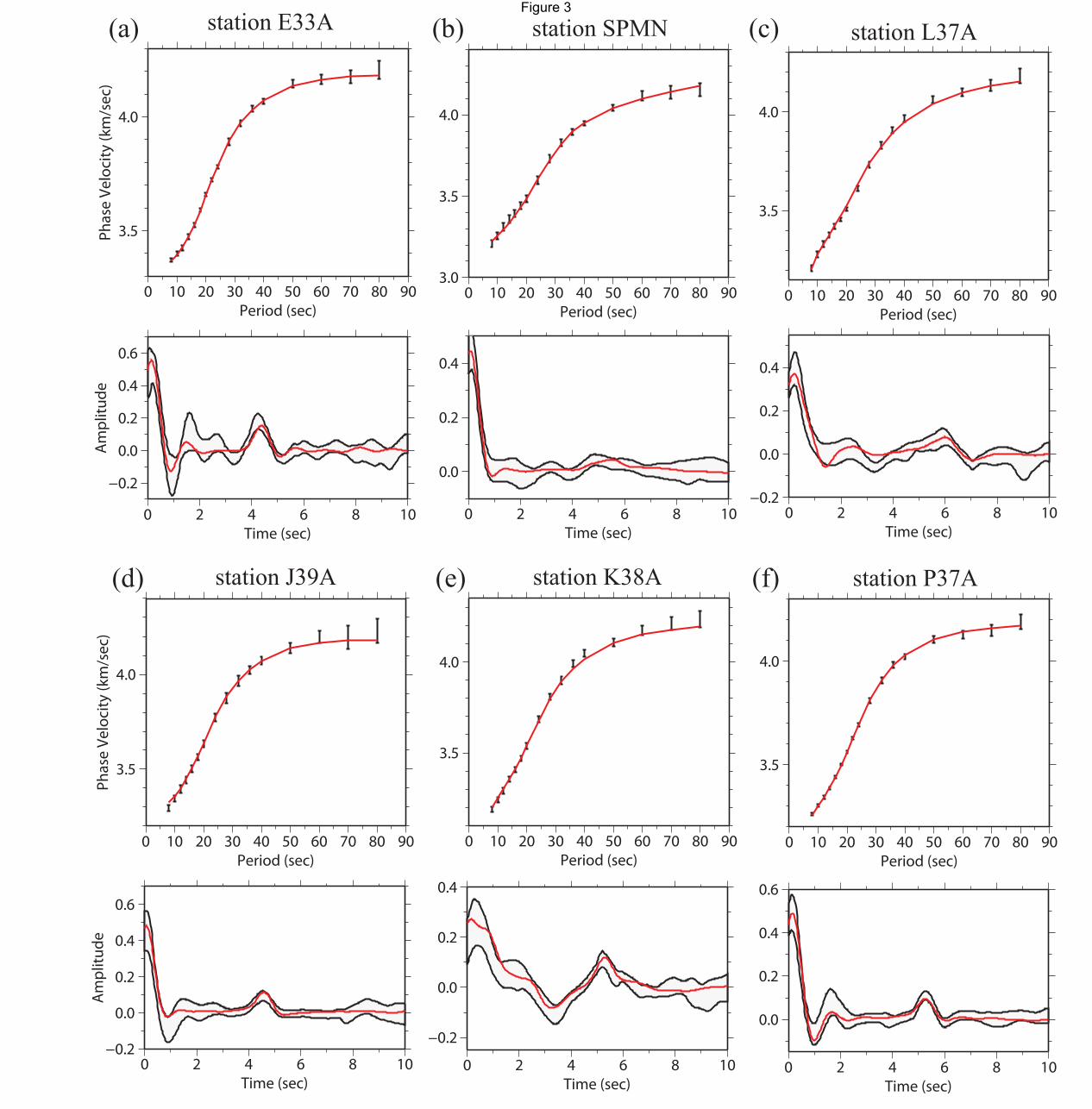
3.0

3.5

4.0

0 10 20 30 40 50 60 70 80 90Period (sec)

3.5

4.0

0 10 20 30 40 50 60 70 80 90Period (sec)

3.5

4.0

Phas

e Ve

loci

ty (k

m/s

ec)

0 10 20 30 40 50 60 70 80 90Period (sec)

3.5

4.0

0 10 20 30 40 50 60 70 80 90Period (sec)

station SPMN station L37A

station J39A station K38A

(a) (b) (c)

(d) (e) (f)

0.0

0.2

0.4

0 2 4 6 8 10Time (sec)

−0.2

0.0

0.2

0.4

0 2 4 6 8 10Time (sec)

−0.2

0.0

0.2

0.4

0.6

Am

plitu

de

0 2 4 6 8 10Time (sec)

−0.2

0.0

0.2

0.4

0 2 4 6 8 10Time (sec)

−0.2

0.0

0.2

0.4

0.6

Am

plitu

de

0 2 4 6 8 10Time (sec)

3.5

4.0Ph

ase

Velo

city

(km

/sec

)

0 10 20 30 40 50 60 70 80 90Period (sec)

station E33A

0.0

0.2

0.4

0.6

0 2 4 6 8 10Time (sec)

3.5

4.0

0 10 20 30 40 50 60 70 80 90Period (sec)

station P37A

Figure 3

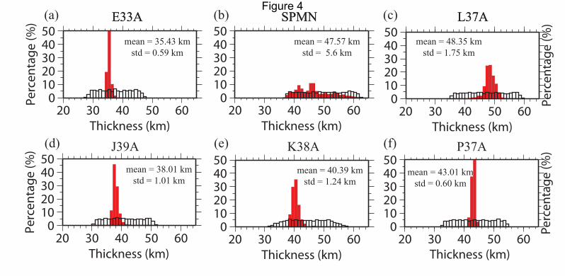
01020304050

Perc

enta

ge (%

)

20 30 40 50 60Thickness (km)

01020304050

20 30 40 50 60Thickness (km)

Perc

enta

ge (%

)

01020304050

Perc

enta

ge (%

)

20 30 40 50 60Thickness (km)

01020304050

20 30 40 50 60Thickness (km)

01020304050

20 30 40 50 60

Perc

enta

ge (%

)

Thickness (km)

E33A SPMN L37AE33A SPMN L37A

J39A K38A P37A

01020304050

20 30 40 50 60Thickness (km)

mean = 35.43 kmstd = 0.59 km

mean = 47.57 kmstd = 5.6 km

mean = 48.35 kmstd = 1.75 km

mean = 38.01 kmstd = 1.01 km

mean = 40.39 kmstd = 1.24 km

mean = 43.01 kmstd = 0.60 km

(a) (b) (c)

(d) (e) (f)

Figure 4

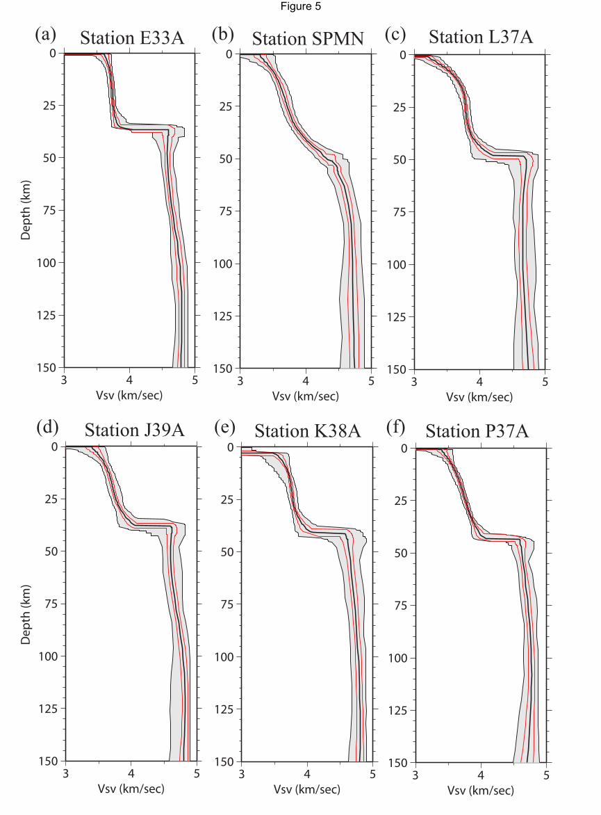
0

25

50

75

100

125

1503 4 5

Vsv (km/sec)

0

25

50

75

100

125

1503 4 5

Vsv (km/sec)

0

25

50

75

100

125

1503 4 5

Vsv (km/sec)

0

25

50

75

100

125

1503 4 5

Vsv (km/sec)

(a) (b) (c) Station SPMN Station L37A

Station J39A Station K38A

0

25

50

75

100

125

150

Dep

th (k

m)

3 4 5Vsv (km/sec)

0

25

50

75

100

125

1503 4 5

Vsv (km/sec)

Station E33A

Station P37A(d) (e) (f)

Dep

th (k

m)

Figure 5

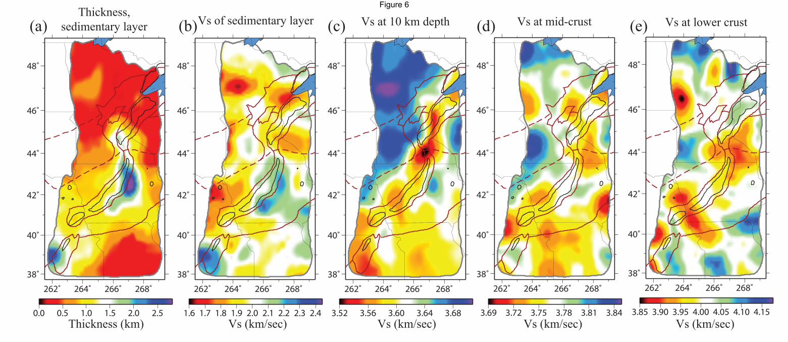
262˚ 264˚ 266˚ 268˚

38˚

40˚

42˚

44˚

46˚

48˚

0.0 0.5 1.0 1.5 2.0 2.5

262˚ 264˚ 266˚ 268˚

38˚

40˚

42˚

44˚

46˚

48˚

1.6 1.7 1.8 1.9 2.0 2.1 2.2 2.3 2.4

262˚ 264˚ 266˚ 268˚

38˚

40˚

42˚

44˚

46˚

48˚

3.52 3.56 3.60 3.64 3.68

262˚ 264˚ 266˚ 268˚

38˚

40˚

42˚

44˚

46˚

48˚

3.69 3.72 3.75 3.78 3.81 3.84

262˚ 264˚ 266˚ 268˚

38˚

40˚

42˚

44˚

46˚

48˚

3.85 3.90 3.95 4.00 4.05 4.10 4.15Thickness (km) Vs (km/sec) Vs (km/sec) Vs (km/sec) Vs (km/sec)

Thickness,sedimentary layer Vs of sedimentary layer Vs at 10 km depth Vs at mid-crust Vs at lower crust(a) (b) (c) (d) (e)

Figure 6

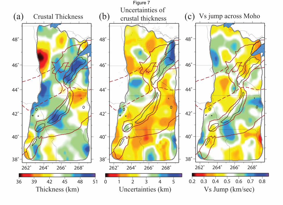
262˚ 264˚ 266˚ 268˚

38˚

40˚

42˚

44˚

46˚

48˚

36 39 42 45 48 51

262˚ 264˚ 266˚ 268˚

38˚

40˚

42˚

44˚

46˚

48˚

0 1 2 3 4 5

262˚ 264˚ 266˚ 268˚

38˚

40˚

42˚

44˚

46˚

48˚

0.2 0.3 0.4 0.5 0.6 0.7 0.8

Thickness (km) Uncertainties (km) Vs Jump (km/sec)

Crustal Thickness Uncertainties of crustal thickness Vs jump across Moho(a) (b) (c)

Figure 7

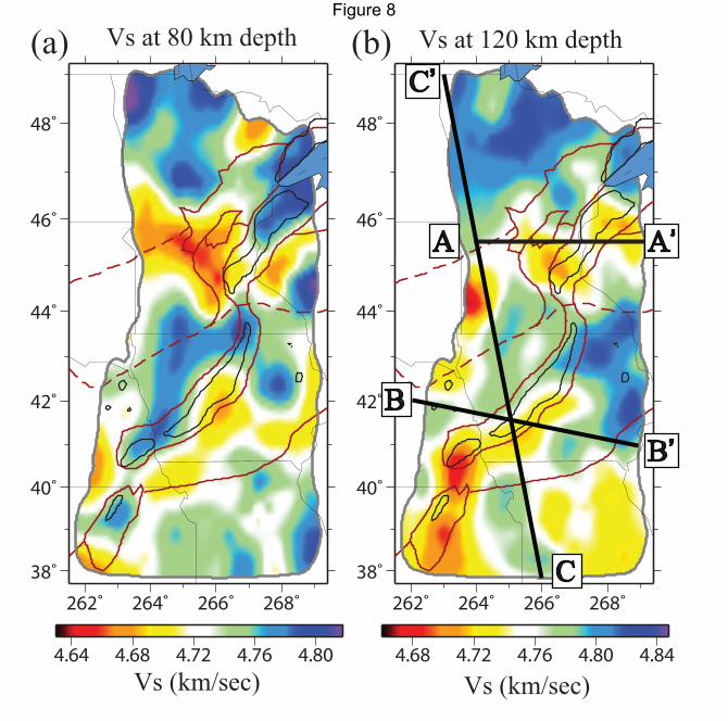
262˚ 264˚ 266˚ 268˚

38˚

40˚

42˚

44˚

46˚

48˚

4.64 4.68 4.72 4.76 4.80

262˚ 264˚ 266˚ 268˚

38˚

40˚

42˚

44˚

46˚

48˚

4.68 4.72 4.76 4.80 4.84Vs (km/sec) Vs (km/sec)

Vs at 80 km depth Vs at 120 km depth(a) (b)

A A’

B

B’

C’

C

Figure 8

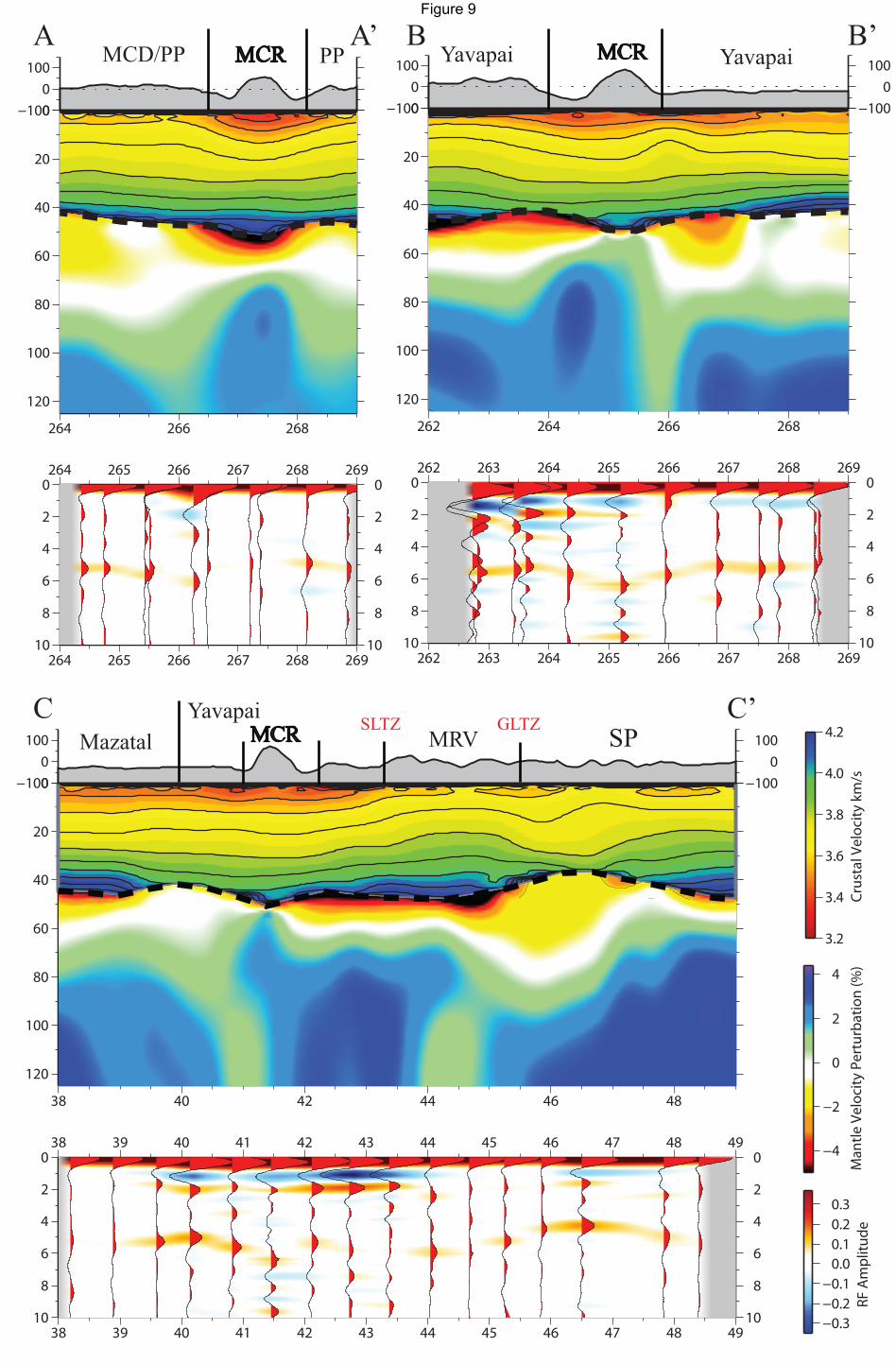
0

20

40

60

80

100

120

264 266 268

−1000

100

0

2

4

6

8

10

0

2

4

6

8

10264 265 266 267 268 269

264 265 266 267 268 269

0

20

40

60

80

100

120

262 264 266 268

−1000

100

−1000

100

0

2

4

6

8

10

0

2

4

6

8

10262 263 264 265 266 267 268 269

262 263 264 265 266 267 268 269

0

20

40

60

80

100

120

38 40 42 44 46 48

−1000

100

−1000

100

3.2

3.4

3.6

3.8

4.0

4.2

Crus

tal V

eloc

ity k

m/s

−4

−2

0

2

4

Man

tle V

eloc

ity P

ertu

rbat

ion

(%)

−0.3−0.2−0.1

0.00.10.20.3

RF A

mpl

itude

0

2

4

6

8

10

0

2

4

6

8

1038 39 40 41 42 43 44 45 46 47 48 49

38 39 40 41 42 43 44 45 46 47 48 49

A A’ B B’MCR MCRYavapai Yavapai

MCR MRVMazatal SPGLTZSLTZYavapai

PPMCD/PP

C C’

Figure 9