Cruise ReportF.S. ALKOR Cruise No. 268

Dates of Cruise: 05.10. to 07.10.2005

Projects:Student course in phys. oceanogr.

Areas of Research: Physical oceanographyPort Call: Warnemunde (05.10.)Institute: IFM-GEOMAR Leibniz-Institut fur Meereswissenschaften an derUniversitat KielChief Scientist: Dr. Johannes KarstensenNumber of Scientists: 11Master: Jan Lass

1

Chapter 1

Scientific personal

Cruise code: AL268Cruise dates: 05.10. – 07.10.2004Port calls: Kiel - Warnemunde - Kiel

Table 1.1: Scientific personal on AL268: IFM-GEOMAR: Leibniz-Institut fur Meereswis-senschaften an der Universitat Kiel, Kiel, Germany; CAU: Cristian Albrechts Universitat Kiel,Kiel, Germany

Name Institute FunctionKarstensen, Johannes IFM-GEOMAR Chief scientistSchmidt, Sunke IFM-GEOMAR Phys. Ocean.Neumann, Uta IFM-GEOMAR Phys. Ocean.Smarz, Christopher IFM-GEOMAR CTD lab.Jacob, Florian CAU studentSchwarzkopf, Franziska CAU studentBehrens, Erik CAU studentBlock, Jana CAU studentDidwischus, Sven-Helge CAU studentSimon, Thorsten CAU studentSchurch, Mark CAU student

Responsible for Report:Johannes Karstensen phone: ++49 (0)431 600-4156Leibniz-Institut fur Meereswissenschaften fax: ++49 (0)431 600-4152DA1

4sternbrooker Weg 20 e-mail: jkarstensen@ifm-geomar.de

24105 Kiel, Germany

2

Chapter 2

Scientific Background

ALKOR cruise AL268 was three day cruise. It was the second cruises in 2005 to maintain thelong term observations in in the western Baltic. The purpose of the cruises was to obtain a rathersynoptic picture of the property distribution and velocities in the western Baltic and to maintaina mooring site at the southeastern opening of the Fehmarn Belt.

In general two section are occupied: one section crossing the Fehmarn Belt (section ’C’)and one section following the deepest topography from about 10◦40 E to 14◦21 E (section ’L’).Along both sections CTD/rosette sampling is performed as well as continuously recording ofcurrent velocities using a vessel mounted ADCP. A mooring site (V431) is maintained (batterychange, data read-out), located at the southeastern opening of the Fehmarn Belt. The mooringconsists of a Workhorse-ADCP (300 kHz), and a self containing CTD (Type MicoCat) mountedin a commercial shield (Flotation Technology).

Besides the scientific motivation, the cruises are utilized for educational purposes. Under-graduate students are introduced into modern observational techniques of physical oceanogra-phy, basics in instrument calibration and interpretation of the observations. In addition it shouldgive the students to experience the work and life at sea in general and last but not least to ex-plore/investigate the Baltic Sea, the ’ocean’ at their back-yard.

3

Chapter 3

Cruise Narrative

10°00’E 10°30’ 11°00’ 11°30’ 12°00’ 12°30’ 13°00’ 13°30’ 14°00’ 14°30’E

54°00’N

54°30’

55°00’

55°30’N

CTD−Stations 05.Okt−07.Okt 2005

Figure 3.1: ALKOR 268 cruise track (black line, based on DATADIS recordings). Red dots arethe CTD stations, black star is the location of the V431 mooring. AL268 had one port call forWarnemunde (05.10.2005)

DAY 1 (Monday, 05.10.2005):We left IFM-GEOMAR pier (Westufer) at 08:00 (all times given in the narrative are ALKOR lo-cal time; MESZ) with 11 ’scientists’ on board, 6 of them were undergraduate students in physicaloceanography, and one in geography.

Most equipment was set-up the day before the cruise (installation of computers, Salinometer).Except the ADCP which was set up during our sail to the first test station. As in earlier years theset up for the ADCP was a bit confusing in respect to COM port settings.

4

The first officer introduced the 7 students into the safety-on-board procedures and guided thestudents through the ship and its facilities. A brief introduction into the program for the next 3days was given next.

A test station was performed to test the HydroBios CTD sonde. The oxygen sensor did notwork and will be sent out for repair to HydroBios during ALKOR winter stop. A nice double-peak in chlorophyll-a was clearly visible.

At around 11:00 we started sampling the first two CTD stations for the zonal section (’L’).A rather large volume of water was collected at the station2, so called ’Substandard’, which willbe used on the following days to monitor the stability of the salinometer. Then the Fehmarnbeltsection (’C’) was sampled with a northward CTD section. After finishing the section, we headedfor the V431 mooring at the southeastern opening of the Fehmarnbelt. On our way we did anADCP section of the Fehmarnbelt heading southward to the 10m depth line with a constant speedof 10 kn. However, apparently there are still problems with the ADCP and the current setting forintensity minimum blanked the deeper part of the data out when the ship was too fast.

In the vicinity of the V431 mooring position a CTD cast was performed for calibration pur-poses. At 16:05 the release command was send and the mooring appeared shortly after that atthe surface. No problems encountered during the mooring recovery.

Warnemunde Passagierkai was reached at 20:05. Customs came aboard and after clearancethose who wanted to leave for a walk could did so.

DAY 2 (Tuesday, 06.10.2005):We left at 08:00 Warnemunde to continue working on the L-section. It was a dusty but sunnymorning and quite sea. At 09:30 we continued with sampling the L-section doing CTD work.

Measurements of the salinity samples (CTD, TSG) from the first day was planned. Samplesare typically stored one day to allow for a temperature adjustment to lab temperature. However,again a problem with the Beckman salinometer appeared through extensive bubbles formation.After clearing the probe container with Mucasol and taking special care on a slow fill up of theprobe-container the measurements went well.

During the day all CTD stations of the L-section east of Warnemunde were occupied. Laststation was measured at about 20:00 and we slowly headed back to finish with work (CTD, moor-ing deployment) west of Warnemunde early Friday morning. In the evening, Jana Block gave atalk on salinity and method of determination in oceanology.

DAY 3 (Wednesday, 07.10.2005):We started early (05:30) with a first CTD station as part of the L-section. Remaining bottlesamples, mainly from the TSG, were analyzed with the Beckman salinometer.

After a calibration cast at the V431 mooring site the mooring V431 was redeployment the11th time. Redeployment was at 07:20 UTC while instruments started recording three hourslater as we did not expect to be at the site that early. The shield had lost paint over the lastyears and it is envisioned to pick up the shield in February 2006 and bring it to IFM-GEOMARfor maintenance. During that time a replacement using a test device Aanderaa (RDCP600) isenvisioned.

After the mooring work we headed for the second hydrographic and ADCP Fehmarnbelt

5

sections. The scientific program was completed at 12:00. The vmADCP was unmounted at13:00. ALKOR reached Kiel (IFM-GEOMAR pier Westufer) at 17:00.

6

Chapter 4

Preliminary results

4.1 Mooring V431: Tenth deployment period

15.Jul 01.Aug 15.Aug 01.Sep 15.Sep 01.Oct2005

−50

0

50 0

5

10

15

20

25

V431, Fehmarnbelt 7−day filtered

Figure 4.1: Mooring V431, upward looking Workhorse 300kHz ADCP - along bathymetry ve-locity (rotated to 132◦). Values are linear averaged over 7 days.

The ADCP is placed at the bottom (about 28m water depth) and measure upward looking.Data points are obtained in 1 m depth cells averaged over 0.5 hours, pinging every 0.5 minutes(30 seconds). A rotation of the velocities by 132◦makes one component parallel and one per-pendicular to the topography. The current component parallel to the topography is shown in theupper figure. Alternating currents of southeast/northwest directions can be seen. The minimumin fluctuations is at about 13 to 14m depth. Note, currents above about 6m depth are influencethrough the surface reflections (and side lopes) and the data is corrupt. The current fluctuationsare mainly related to the wind forcing.

An interesting feature in the temperature and salinity time series are the high frequency fluc-tuations which occur order every 5 days or so. The fluctuations occurs predominately after the

7

01.Aug 15.Aug 01.Sep 15.Sep 01.Oct2005

22

23

24

25

26

27

Sal

init

y

01.Aug 15.Aug 01.Sep 15.Sep 01.Oct2005

8

9

10

11

12

13

Tem

per

atu

re

Figure 4.2: Time series salinity (upper) and temperature (lower) from the 10th deployment pe-riod.

peak salinity was reached in later June/early July which is also the time after the strongest in-crease in density.

8

1999 2000 2001 2002 2003 2004 200515

20

25

30

salin

ity

1999 2000 2001 2002 2003 2004 20050

5

10

15

tem

pera

ture

[°C

]

Figure 4.3: Time series salinity (upper) and temperature (lower) in reference to the mean annualcycle (black line) of Mooring V399 (since 23. Feb. 1999) and V431 (since 8. May 2002),Fehmarnbelt, western Baltic.

The temperature and salinity time series shown even at the bottom a pronounced seasonalcycle. Highest temperatures of up to 15◦C occur in early October. The highest salinity appearsto be end of June with a second, smaller peak late January. The summer peak is related to theentrainment of North Sea Water at mid depth while the winter peak is a results of occasionalNorth Sea water inflow, the deep Baltic proper ventilation events.

9

1999 2000 2001 2002 2003 2004 2005−5

0

5

salin

ity a

nom

aly

1999 2000 2001 2002 2003 2004 2005−2

−1

0

1

2

tem

pera

tur

anom

aly

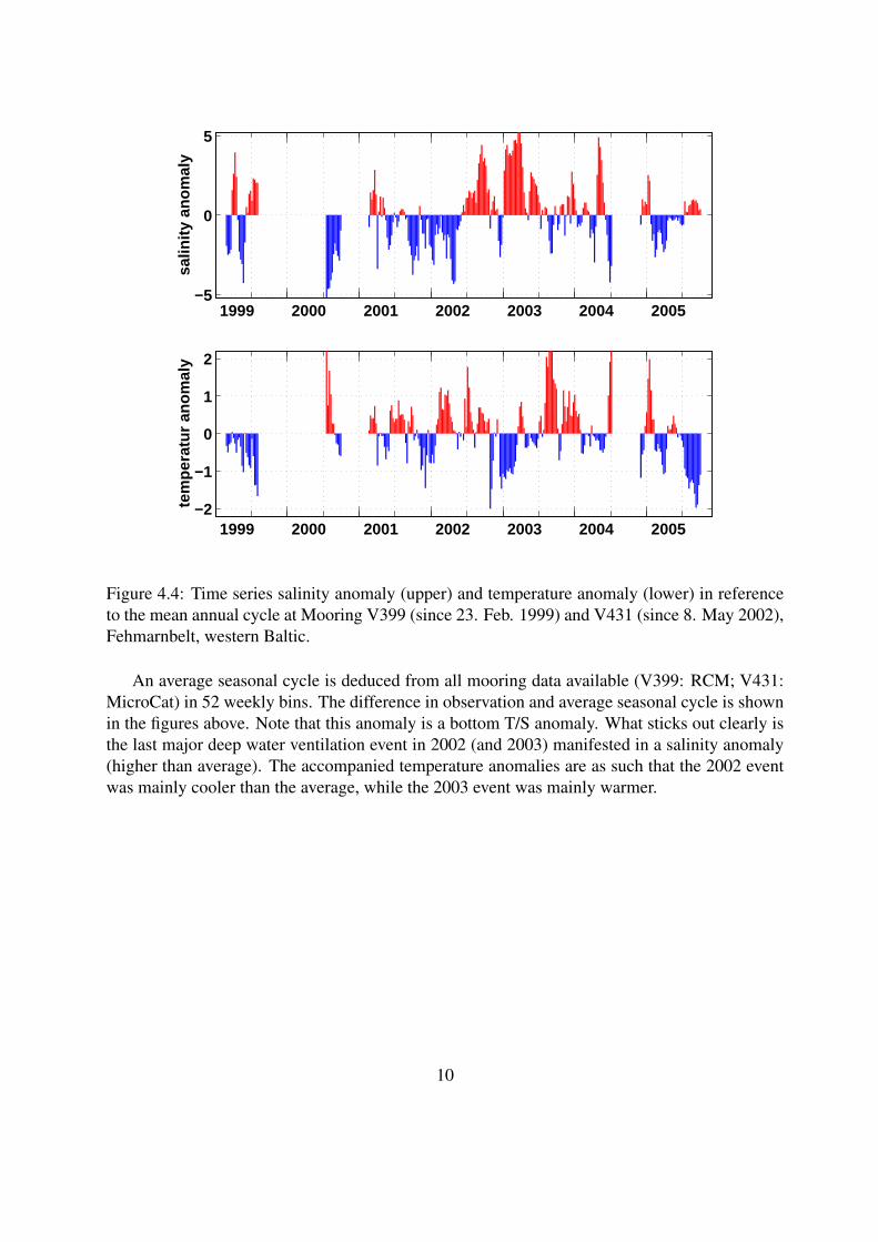
Figure 4.4: Time series salinity anomaly (upper) and temperature anomaly (lower) in referenceto the mean annual cycle at Mooring V399 (since 23. Feb. 1999) and V431 (since 8. May 2002),Fehmarnbelt, western Baltic.

An average seasonal cycle is deduced from all mooring data available (V399: RCM; V431:MicroCat) in 52 weekly bins. The difference in observation and average seasonal cycle is shownin the figures above. Note that this anomaly is a bottom T/S anomaly. What sticks out clearly isthe last major deep water ventilation event in 2002 (and 2003) manifested in a salinity anomaly(higher than average). The accompanied temperature anomalies are as such that the 2002 eventwas mainly cooler than the average, while the 2003 event was mainly warmer.

10

4.2 Meteorological observationsGeneral weather situation (figure 4.5): During the 3 days of our expedition, there was a highpressure system over the whole Baltic Sea domination the weather. This system was movingeastwards very slowly.

12:00 00:00 12:00 00:00 12:001000

1005

1010

1015

1020

1025

1030

1035

1040

1045

1050air−pressure from 05.10. − 7.10.05

time in UTC

air−

pres

sure

in h

Pa

Figure 4.5: Surface pressure distribution 05. Oct to 07.Oct. 2005 (UKMO-Bracknell, UK).Lower left: pressure readings during AL268.

The pressure in the centre was stable between 1034 and 1036 hPa at the surface ((figure 4.5,lower left)). Due to the wide distance between the isobars, the weather conditions were verystable during the whole cruise. The cloud cover was always 0/8, the air temperature was varyingbetween 10 and 16◦C and the wind was mostly blowing between 5 to 10 m/s (4-5 Bft.) fromeasterly directions.

The dry air temperature graph (figure 4.6, left, blue) shows a typical diurnal cycle: Thelowest temperatures are measured in the early morning around 6 am, just before sunrise. A quickincrease after noon with a maximum temperature around 2 pm of about 15◦C. In the afternoonand evening there is a slow decrease of temperature till the temperature reaches its minimum inthe early morning again. The difference in temperature between day and night is about 5◦C in

11

the first night and 2.5◦C in the second night. This can be explained by the fact that we stayedin harbour during the first night, while we were on sea during the second night. Because thewater mass doesn’t cool so fast during the night as the landmass, the air temperature over seais less extreme. The same plot shows also the graph of the humid temperature (figure 4.6, left,green). It shows a parallel course to the dry air temperature, but some degrees below, because ofthe reduction of the temperature due to the evaporation at the wet thermometer. So, we expect amore or less constant relative humidity during this period of time (figure 4.6, right).

12:00 00:00 12:00 00:00 12:000

2

4

6

8

10

12

14

16

18

20

time in UTC

tem

pera

ture

in °

C

dry and wet air temperature from 05.10. − 07.10.05

dry temperaturewet temperature

12:00 00:00 12:00 00:00 12:000

10

20

30

40

50

60

70

80

90

100relative humidity from 05.10. − 7.10.05

time in UTC

rela

tive

hum

idity

in %

Figure 4.6: Timeseries of dry and wet temperature (left) and relative humidity (right). Data gapbetween 7 pm on 5/10/2005 and 5 am on 6/10/2005 (Harbour call Warnemunde).

The water temperature is quite constant during the first day, while it is more variable duringthe second and third day. In contrast to the air temperature, the water temperature (Figure 4.6,left) has a less extreme diurnal cycle varying by about 1.5◦C. Small scale variability is probablydue to the ship is crossing different water masses. During the first day the rather constant watertemperature is due ot the shallow waters between Kieler Forde and Warnemunde. Here highertemperature than in the open Baltic are expected. So due to our route, we would expect a decreaseof the water temperature during the first two hours, but the influence of the course of day isworking against this trend.

The wind speed is roughly proportional to the distance between the isobars. The rather con-stant pressure during the cruise caused a rather constant wind speed during the cruise with speedsbetween 5 and 10 m/s. We can difference three parameters that determine the wind speed duringthese three day. First there is a gradient wind from 5 to 7 m/s, that changes with the positionof the high. Second we can observe an thermal influence, that increases the wind speed duringthe afternoons 2 to 3 m/s. Third, the decrease of wind speed in the harbour around 5 pm mustbe explained by the shelter of the landmasses, that slow the wind speed down. As the water isabout one degree higher than the air temperature there is a constant ’heating’ at the air/sea inter-face (negative sensible heat) and local upward movement of the air masses at the interface. Thisgenerates a low pressure tendency within the high pressure system.

The plot of the wind direction shows an average value of 100◦, so almost east. During the firstday there is a north component, during the second day, there is a south component to observe.The third day shows a stable direction of 100◦. The big peaks in the graph don’t show the real

12

12:00 00:00 12:00 00:00 12:000

2

4

6

8

10

12

14

16

18

20water temperature from 05.10. − 7.10.05

time in UTC

tem

pera

ture

in °

C

12:00 00:00 12:00 00:00 12:000

10

20

30

40

50

60

70

80

90

100relative humidity from 05.10. − 7.10.05

time in UTC

rela

tive

hum

idity

in %

Figure 4.7: Timeseries of water temperature (left) and relative humidity. Data gap between 7 pmon 5/10/2005 and 5 am on 6/10/2005 (Harbour call Warnemunde).

wind direction. They are exactly at the same position as we did our stations for the CTDs. Weexplain these anomalies with the turning of the vessel during the stations and the time delay ofthe instruments. The general wind direction changing from little less than 100◦to little more than100◦and back to 100◦has to be explained by the southeast moving of the high, that changes theorientation of the isobars, which determines the direction of the gradient wind.

12:00 00:00 12:00 00:00 12:000

5

10

15windspeed from 05.10. − 7.10.05

time in UTC

win

dspe

ed in

m/s

12:00 00:00 12:00 00:00 12:000

50

100

150

200

250

300

350

winddirection from 05.10. − 7.10.05

time in UTC

in m

eteo

rolo

gica

l deg

rees

Figure 4.8: Timeseries of wind speed (left) and wind direction (right). Data gap between 7 pmon 5/10/2005 and 5 am on 6/10/2005 (Harbour call Warnemunde).

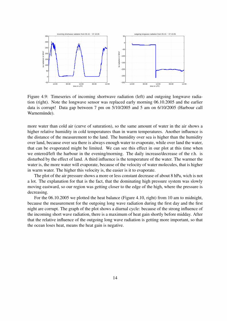
The incoming short wave radiation (ISWR) resamples the diurnal cycle of the temperaturewith a maximum around 11 UTC (noon local time). Due to the late season and the short days,there is a steep increase during the morning and a steep decrease in the afternoon. The maximumISWR is around 280 W m−2. This is a lot less than the climatological maximum in summer(360 W m−2), because the suns radiation approaches the surface in a smaller angle.

The graph of the relative humidity stays very high >80% during all the measured time period.In the course of day you can observe a change by daytime. Due to the cooling in the night, therelative humidity increases, while it decreases in daytime. That’s because warm air can hold

13

12:00 00:00 12:00 00:00 12:00−50

0

50

100

150

200

250

300

350incoming shortwave radiation from 05.10. − 07.10.05

time in UTC

sw r

adia

tion

in W

/m²

12:00 00:00 12:00 00:00 12:00−300

−250

−200

−150

−100

−50

0

50outgoing longwave radiation from 05.10. − 07.10.05

time in UTC

lw r

adia

tion

in W

/m²

Figure 4.9: Timeseries of incoming shortwave radiation (left) and outgoing longwave radia-tion (right). Note the longwave sensor was replaced early morning 06.10.2005 and the earlierdata is corrupt! Data gap between 7 pm on 5/10/2005 and 5 am on 6/10/2005 (Harbour callWarnemunde).

more water than cold air (curve of saturation), so the same amount of water in the air shows ahigher relative humidity in cold temperatures than in warm temperatures. Another influence isthe distance of the measurement to the land. The humidity over sea is higher than the humidityover land, because over sea there is always enough water to evaporate, while over land the water,that can be evaporated might be limited. We can see this effect in our plot at this time whenwe entered/left the harbour in the evening/morning. The daily increase/decrease of the r.h. isdisturbed by the effect of land. A third influence is the temperature of the water. The warmer thewater is, the more water will evaporate, because of the velocity of water molecules, that is higherin warm water. The higher this velocity is, the easier is it to evaporate.

The plot of the air pressure shows a more or less constant decrease of about 8 hPa, wich is nota lot. The explanation for that is the fact, that the dominating high pressure system was slowlymoving eastward, so our region was getting closer to the edge of the high, where the pressure isdecreasing.

For the 06.10.2005 we plotted the heat balance (Figure 4.10, right) from 10 am to midnight,because the measurement for the outgoing long wave radiation during the first day and the firstnight are corrupt. The graph of the plot shows a diurnal cycle: because of the strong influence ofthe incoming short wave radiation, there is a maximum of heat gain shortly before midday. Afterthat the relative influence of the outgoing long wave radiation is getting more important, so thatthe ocean loses heat, means the heat gain is negative.

14

12:00 00:00 12:00 00:00 12:00−35

−30

−25

−20

−15

−10

−5

0

5

10

15sensible heat flux from 05.10. − 07.10.05

time in UTC

heat

flux

in W

/m²

12:00 00:00 12:00 00:00 12:00

−200

−150

−100

−50

0

latent heat flux from 05.10. − 07.10.05

time in UTC

heat

flux

in W

/m²

12:00 00:00

−300

−200

−100

0

100

200

300heat balance from 06.10.2005

time in UTC

heat

gai

n in

W/m

²

Figure 4.10: Sensible (left), latent (center) heat flux and heat balance for the period were reliablelongwave radiation data was available (right).

15

4.3 Hydrographic and currents along C and L section

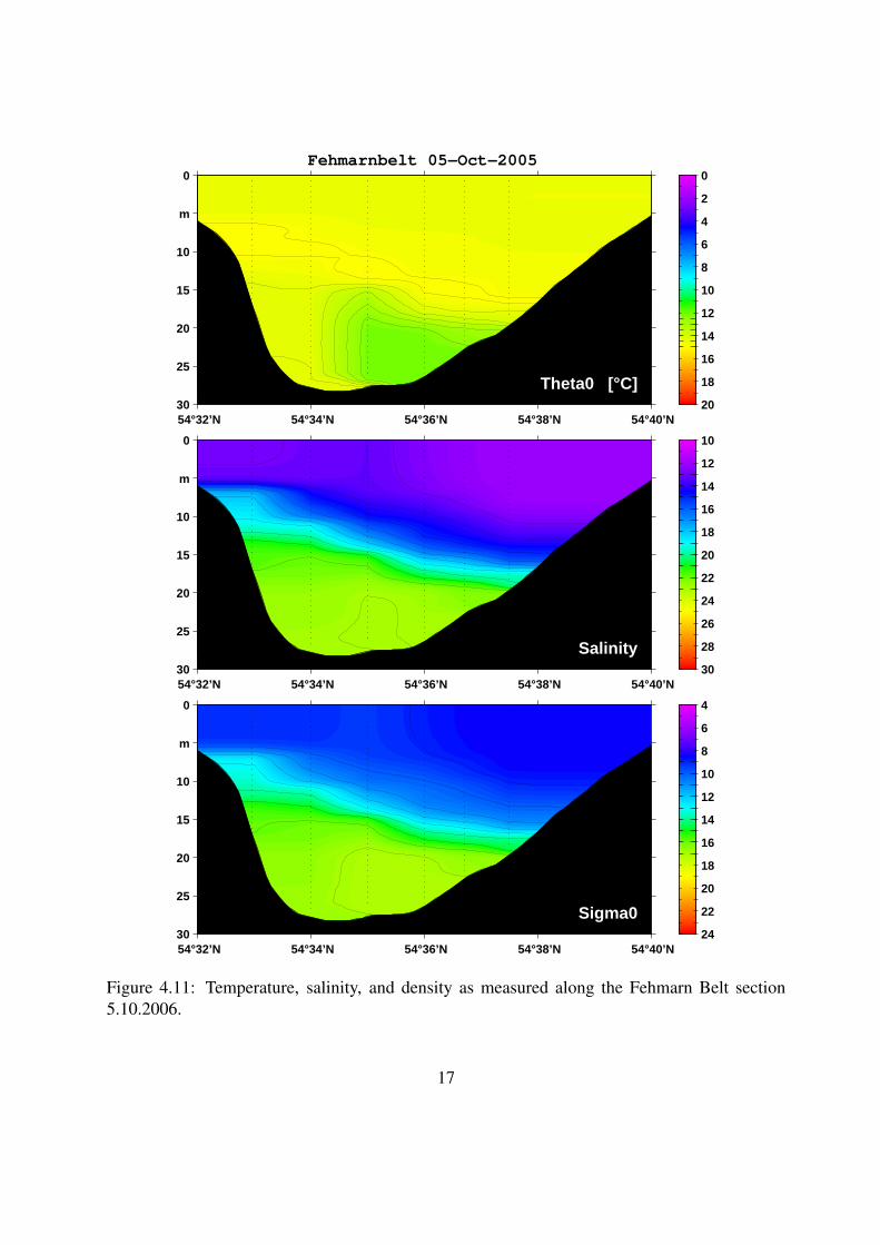
4.3.1 Fehmarnbelt (C section)The temperature distribution (figure 4.11, upper) across Fehmarnbelt is quite homogeneously.There is a warm layer in the upper five meters in the south and the upper ten meters in the north,with temperatures about 14.7◦C. Beneath, there is a layer about five meters with the temperatemaximum at about 15◦C. From there to the ground the temperature decreases continuously. Thetemperature minimum at the deepest point in the Fehmarnbelt is about 12.2◦C.

The salinity distribution (figure 4.11, middle) shows horizontal layers in which the salinityincreases with depth. At the surface the salinity is about 12 to 13 and on the ground about 22 to23. There is a slope from south to north as earlier seen in the temperature distribution too.

The density (figure 4.11, lower) shows a stable distribution with denser water at about 19 kg m−3 onthe ground and less dense water at about 9 kg m−3 above. It is very similar and consequently de-termined by the salinity distribution. The south north/slope here is also visible.

The chlorophyll-a concentration (figure 4.11, upper) in the upper five meters is about 1 to2. In the following five meters it increases to 4.5. This is dependent on temperature, whichhas the upper limit of its maximum in this layer. Beneath, the chlorophyll-a in the middle ofFehmarnbelt decreases to the ground. In the south there is a decrease across the temperaturemaximum layer and another maximum in chlorophyll-a beneath it. From thirteen meter depthto the ground there is nearly no chlorophyll-a. In the north, the chlorophyll-a maximum ends ateleven meter depth and at about sixteen meters there again is a slight increase. The increase atdepth is approximately due to the vertical mixing associated with a deepening of the mixed layerand nutrient enrichment from the North Sea water core. The upper waters are already depleted.

16

Theta0 [°C]

Fehmarnbelt 05−Oct−2005

54°32’N 54°34’N 54°36’N 54°38’N 54°40’N

0

m

10

15

20

25

30

0

2

4

6

8

10

12

14

16

18

20

Salinity

54°32’N 54°34’N 54°36’N 54°38’N 54°40’N

0

m

10

15

20

25

30

10

12

14

16

18

20

22

24

26

28

30

Sigma0

54°32’N 54°34’N 54°36’N 54°38’N 54°40’N

0

m

10

15

20

25

30

4

6

8

10

12

14

16

18

20

22

24

Figure 4.11: Temperature, salinity, and density as measured along the Fehmarn Belt section5.10.2006.

17

Chl_a [µg/l]

Fehmarnbelt 05−Oct−2005

54°32’N 54°34’N 54°36’N 54°38’N 54°40’N

0

m

10

15

20

25

30

0

1

2

3

4

Salinity

54°32’N 54°34’N 54°36’N 54°38’N 54°40’N

0

m

10

15

20

25

30

10

12

14

16

18

20

22

24

26

28

30

Sigma0

54°32’N 54°34’N 54°36’N 54°38’N 54°40’N

0

m

10

15

20

25

30

4

6

8

10

12

14

16

18

20

22

24

Figure 4.12: Chlorophyll-a, salinity, and density as measured along the Fehmarn Belt section5.10.2006.

18

4.3.2 Zonalsection (L section)In the west of Fehmarnbelt the temperature (figure 4.13, upper) is nearly the same with about15◦C across the whole water column. From Fehmarnbelt (11.2◦E) to 12.5◦E the temperature de-creases eastward and with depth. From 12.5◦E to 13.5◦E it increases eastward and decreases withdepth. At a depth of fourteen meters at 12.7◦E there is a minimum in temperature with about6.5◦C. From 13.5◦E to 14.3◦E the temperature in the upper 18 meters is nearly homogeneouswith about 15◦C. From 13.5◦E to 14◦E the temperature decreases from 18 to 32 meters depth to10.5◦C and from there onto the ground there again is an increase of 2◦C. From 14◦E to 14.3◦Ethe temperature decreases to its minimum with about 5◦C at 27 meter depth.

The salinity distribution (figure 4.13, middle) can be subdivided into two sections: western of12.7◦E and eastern of 12.7◦E. In the western part at the surface there is a salinity of about 10 to14 decreasing eastward and across the water column increasing to its maximum at about 23. Inthe eastern part all the water above 20 meters depth has a very low salinity at about 7. Beneath,it increases slightly to 13 on the ground. The saltier water in the deeper west part has its originin the north sea. It cannot pass the threshold at 12.5◦E.

Density in general is dependent on temperature, salinity and pressure. Here, the density dis-tribution (figure 4.13, lower) is very similar to the distribution of salinity, with its maximum atabout 1018 kg m−3 and its minimum at about 1005 kg m−3 . In density there is the answer, whythe water of the north sea cannot pass the threshold. It is too dense and with that too heavy.

The subdivision can be used for the chlorophyll-a distribution (figure figure 4.14, upper), too.In the western part there are a few places with rather high chlorophyll-a values up to 5. In theeastern part the chlorophyll-a concentration decreases with depth from 2.5 at the surface to 0.5on the ground.

19

Theta0 [°C]

Fehmarnbelt − ArkonaBasin, 05.Okt−07.Okt 2005

11°00’N 11°30’N 12°00’N 12°30’N 13°00’N 13°30’N 14°00’N

0

m

20

30

40

50

0

2

4

6

8

10

12

14

16

18

20

Salinity

11°00’N 11°30’N 12°00’N 12°30’N 13°00’N 13°30’N 14°00’N

0

m

20

30

40

50

6

8

10

12

14

16

18

20

22

24

Sigma0

11°00’N 11°30’N 12°00’N 12°30’N 13°00’N 13°30’N 14°00’N

0

m

20

30

40

50

4

6

8

10

12

14

16

18

20

22

24

Figure 4.13: Chlorophyll-a, salinity, and density as measured along the Fehmarn Belt section5.10.2006.

20

Chl_a [µg/l]

Fehmarnbelt − ArkonaBasin, 05.Okt−07.Okt 2005

11°00’N 11°30’N 12°00’N 12°30’N 13°00’N 13°30’N 14°00’N

0

m

20

30

40

50

0

1

2

3

4

Salinity

11°00’N 11°30’N 12°00’N 12°30’N 13°00’N 13°30’N 14°00’N

0

m

20

30

40

50

6

8

10

12

14

16

18

20

22

24

Sigma0

11°00’N 11°30’N 12°00’N 12°30’N 13°00’N 13°30’N 14°00’N

0

m

20

30

40

50

4

6

8

10

12

14

16

18

20

22

24

Figure 4.14: Chlorophyll-a, salinity, and density as measured along the Fehmarn Belt section5.10.2006.

21

Chapter 5

Equipment/instruments

5.1 Mooring V431Mooring deployment site V431 is located in the military zone of Marienleuchte at the southeast-ern opening of the Fehmarnbelt. Water depth is about 29m. V431 consists of a Workhorse ADCP(300kHz; Serial number 1962) and a self containing T/S recorder of type SBE-MicroCat (serialnumber 2936).

Table 5.1: V431: Summary on 10th recovery and 11th deployment of trawl resistant bottommooring V431.

date; time (UTC) latitude longitude depth comment05.10.2005; 14:20 Recovery.07.10.2005; 07:20 54◦31.33’N 11◦18.21’E 28.2 m 11th Redeployment.

5.2 CTD/Rosette and Salinometer

5.2.1 CTD

A Hydro-Bios CTD was used during the cruise. Last lab calibration indicated an accuracy oforder 0.001 K in temperature.

5.2.2 Beckmann Salinometer

The robust and portable Beckmann Salinometer was used to analyse the water samples. TheBeckman Salinometer uses an inductive method to measure the salinity of a water sample. Toachieve good measurements (precision order 0.0008/accuracy order 0.003) the samples are storedfor 24h in the lab to allow for a temperature adjustment.

22

Up to three repeat measurements have been performed on each sample (CTD, TSG, Substan-dard) or until the difference in salinity (which is determined through the ’Salino’ program thatreads out the data from the Beckman Salinometer via a COM port connector) is less than 0.01.

Before the first measurement the instrument is calibrate against standard seawater. After asubstandard is used which is a large volume of Baltic Sea Water collected at the first station.Ideally this should stay constant during all measurements. For our measurements (Figure 5.1) nosystematic trend in the difference between subsequent substandard measurements can be seen.

The repeat measurement suggest the salinities are determined better than order 0.02.

0 5 10 15 20 25−0.1

−0.08

−0.06

−0.04

−0.02

0

0.02

0.04

shift of the Beckmann salinometer (substandard)

hour after first measurement

dS

Figure 5.1: Difference in substandard measurements during cruise

5.2.3 Salinity measurements

Some typical salinity profiles are shown in the following that document the strong variability andprovide examples for what will be discussed in reference to differences in the salinity determi-nation using TSG, bottle samples and CTD.

Profile 5 (Figure 5.2, left) shows very good the water mass distribution of the western balticsea. The upper water mass has a low salinity, it comes from the northern baltic sea. There thewater-inflow from rivers and precipitation is much higher than evaporation. In the lower watermass the salinity is much higher. It comes from the north sea. Because of that you can see a

23

10 12 14 16 18 20 22 24−30

−25

−20

−15

−10

−5

0

salinity

dept

h/m

salinity profile Nr.05

CTD−profileCTD when samplingthermosalinographrosette−bottleTSG−sample

7 8 9 10 11 12 13 14 15 16−45

−40

−35

−30

−25

−20

−15

−10

−5

0

salinity

dept

h/m

salinity profile Nr.16

CTD−profileCTD when samplingthermosalinographrosette−bottleTSG−sample

Figure 5.2: Salinity at station 5 (left) and 19 (right)

halocline.Profile 16 (Figure 5.2, right) is from a station more eastern. There the water inflow from thenorth sea is not as strong as in profile 5.

5.2.4 Differences and errors: CTD versus Bottle samples

As one can see in Figure ??,the salinity determined with different instruments or methods pro-vides for a certain depth provide rather different results. Besides the differences between up- anddown-cast of the CTD other difference have been identified.

There is a huge different between the TSG- and the CTD-values (Figure 5.3). The TSG-values are mostly lower than the CTD ones. As the Salinometer agrees well with the CTDsalinity, the difference is caused by the TSG.

Because the CTD-values were used for the evaluation of this cruise, it is most important toknow about the errors of this measurement. CTD samples from different depth have been col-lected during the cruise and later analysed with the Beckmann-Salinometer (Figure 5.4). Surfacenear salinities are quite similar, this is also true for samples near the bottom. Largest differencesoccur where the salinity gradient is strong (halocline).

The error is defined as the difference between CTD-value and Beckmann-value of the bottle,and an uncertainty of the error which is the difference between mean salinity over the columnand the CTD-measurement. Figure 5.5 shows that error as well as the uncertainty is largest atthe halocline.We suggest this ’error’ is mainly caused by the differences in volumes of water which are underconsideration: Because the height of the water sample bottle is about 85cm the sample analysedwith the Beckman Salinometer is the average salinity over the height of the rosette-bottle. TheCTD in contrast measures the salinity at very small volume occupied by its conductivity cell(Figure 5.5). Consequently the Beckman salinometer values (the bottle samples) are averagesalinities over the height of the rosette-bottle (85cm) and compared it with the CTD-value fromasingle point.

24

0 2 4 6 8 10 12 14 16−2

0

2salinity−difference between TSG−measurement and TSG−samples with salinometer

profile−Nr.

diffe

renc

e in

ppt

0 2 4 6 8 10 12 14 16−1

0

1salinity−difference between TSG−samples with salinometer and ctd−measurement

profile−Nr.

diffe

renc

e in

ppt

0 2 4 6 8 10 12 14 16−2

0

2salinity−difference between TSG−measurement and ctd−measurement

profile−Nr.

diffe

renc

e in

ppt

Figure 5.3: Comparison of salinity from TSG-, CTD-measurements and TSG-samples

25

−6 −4 −2 0 2 4−60

−40

−20

0S−difference mean

dS−6 −4 −2 0 2 4

−60

−40

−20

0S−difference median

dS

dept

h in

m/p

ress

ure

in d

bar

−6 −4 −2 0 2 40

10

20

30S−difference mean

dS−6 −4 −2 0 2 40

10

20

30S−difference median

dS

salin

ity

−6 −4 −2 0 2 40

5

10

15

20S−difference mean

dS−6 −4 −2 0 2 40

5

10

15

20S−difference median

dS

tem

pera

ture

Figure 5.4: Difference in salinity from CTD(mean, median) and CTD-rosette(Beckmann) againstdepth, salinity and temperature

−50 −40 −30 −20 −10 0 10−12

−10

−8

−6

−4

−2

0

2

4

6 mean difference with errorbar

depth in m

salin

ity

Figure 5.5: Error and uncertainty of error in CTD-salinity measurement (left), schematic ofposition of the CTD in comparison to the sample bottle (right).

26

5.3 Underway Measurements

5.3.1 DatadisALKOR has a central data collection system, called DATADIS. Here data from a number ofsources (sensors) is merged into a single file which can be used from other devices or/and storedfor later processing. The Maritec Engineering DATADIS includes now UTC GPS based timestamps. However, SIMRAD depth soundings are still not available.

5.3.2 NavigationALKOR has a GPS navigational system as well as a gyro compass available. Data is fed intoDATADIS and from their available for other devices. For the use with the ADCP system a con-verter is needed that ’translates’ the DATADIS string into a ADCP readable string (for headingonly).

Two new monitor in the wet lab and in the dry lab allow to follow the navigation (way point,current position, distance and time to way point, ...) and to see the information embedded into anavigational map. This is a great new feature and very much appreciated.

5.3.3 Meteorological DataALKOR is equipped with meteorological sensors measuring air temperature, wind (speed and di-rection), wet-temperature, air-pressure, long and shortwave radiation. During our cruise Christo-pher Smarz installed a new EPLAB (Eppley Laboratory, Inc.) Precision Infrared Radiometer(Model PIR). The PIR could only be connected in a mode that does not consider the case tem-perature which results in a lower precision. There is a need for a battery change every 4 to 6month (Feb. to Apr. 2006).

5.3.4 Echo sounderDuring AL 268 the ER 60 SIMRAD echo sounder was switched on but the data not recorded.

5.3.5 ThermosalinographThe thermosalinograph (TSG) on ALKOR is permanently installed at about 4m depth and aS/MT 148 type of Salzgitter Elektronik GmbH. TSG data is directly fed into the DATADIS.Calibration was done after the cruise after analysis of bottle samples.

5.3.6 Vessel mounted ADCPA 300 kHz workhorse ADCP from RD Instruments was mounted in the ships hull. The vmADCPis used with bottom tracking mode. Navigational data comes from the DATADIS system of

27

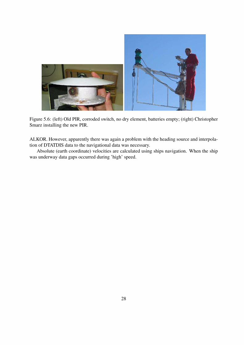
Figure 5.6: (left) Old PIR, corroded switch, no dry element, batteries empty; (right) ChristopherSmarz installing the new PIR.

ALKOR. However, apparently there was again a problem with the heading source and interpola-tion of DTATDIS data to the navigational data was necessary.

Absolute (earth coordinate) velocities are calculated using ships navigation. When the shipwas underway data gaps occurred during ’high’ speed.

28

Chapter 6

Acknowledgement

Herzlichen Dank an Kapitı¿12n Jan Lass und die gesamten Besatzung der ALKOR fur ihre pro-

fessionelle Unterstutzung und die nette Atmosphare an Bord.

29

Chapter 7

Appendix

Station table Station #, Year, Month, Day, Hour, Minute, lat, latmin, long, longmin, depth, Prak-tikum station #

01 2005 10 05 08 36 54 34.00 10 39.93 21.0 0102 2005 10 05 09 40 54 36.52 10 55.01 23.0 0203 2005 10 05 10 24 54 35.49 11 04.97 31.0 0304 2005 10 05 11 02 54 32.96 11 09.73 18.0 0405 2005 10 05 11 25 54 33.99 11 11.03 28.0 0506 2005 10 05 11 45 54 34.99 11 12.47 28.0 0607 2005 10 05 12 03 54 36.00 11 13.48 27.5 0708 2005 10 05 12 21 54 36.70 11 14.46 24.0 0809 2005 10 05 12 36 54 37.50 11 15.48 20.0 0910 2005 10 05 13 45 54 31.39 11 18.45 28.0 1011 2005 10 06 07 25 54 24.01 12 10.00 21.0 1512 2005 10 06 08 27 54 31.99 12 18.01 23.5 1613 2005 10 06 09 26 54 38.02 12 30.01 18.0 1714 2005 10 06 10 23 54 43.26 12 42.50 21.0 1815 2005 10 06 11 28 54 48.50 12 54.98 22.5 18.516 2005 10 06 13 46 54 55.00 13 29.97 47.4 1917 2005 10 06 16 01 54 47.00 13 59.97 39.0 20

30