Embed Size (px)
Citation preview

Cross Ranking of Cities and Regions: Population
vs. Income
Roy Cerqueti1,∗ and Marcel Ausloos2,3
1 University of Macerata, Department of Economics and Law,via Crescimbeni 20, I-62100, Macerata, Italy
e-mail address: [email protected]
2eHumanities group†,Royal Netherlands Academy of Arts and Sciences,
Joan Muyskenweg 25, 1096 CJ Amsterdam, The Netherlands
3GRAPES‡,rue de la Belle Jardiniere 483, B-4031, Angleur Liege, Belgium
e-mail address: [email protected]
Abstract
This paper explores the relationship between the inner economicalstructure of communities and their population distribution through arank-rank analysis of official data, along statistical physics ideas withintwo techniques. The data is taken on Italian cities. The analysis is per-formed both at a global (national) and at a more local (regional) levelin order to distinguish ”macro” and ”micro” aspects. First, the rank-sizerule is found not to be a standard power law, as in many other studies,but a doubly decreasing power law. Next, the Kendall τ and the Spear-man ρ rank correlation coefficients which measure pair concordance andthe correlation between fluctuations in two rankings, respectively, - as acorrelation function does in thermodynamics, are calculated for findingrank correlation (if any) between demography and wealth. Results shownon only global disparities for the whole (country) set, but also (regional)disparities, when comparing the number of cities in regions, the numberof inhabitants in cities and that in regions, as well as when comparing theaggregated tax income of the cities and that of regions. Different outliersare pointed out and justified. Interestingly, two classes of cities in thecountry and two classes of regions in the country are found. ”Commonsense” social, political, and economic considerations sustain the findings.More importantly, the methods show that they allow to distinguish com-munities, very clearly, when specific criteria are numerically sound. A
∗Corresponding address: University of Macerata, Department of Economics and Law, viaCrescimbeni 20, I-62100, Macerata, Italy. Tel.: +39 0733 258 3246; Fax: +39 0733 258 3205.Email: [email protected]†Associate Researcher‡Group of Researchers for Applications of Physics in Economy and Sociology
1
arX
iv:1
506.
0241
4v1
[q-
fin.
EC
] 8
Jun
201
5

specific modeling for the findings is presented, i.e. for the doubly de-creasing power law and the two phase system, based on statistics theory,e.g., urn filling. The model ideas can be expected to hold when similarrank relationship features are observed in fields. It is emphasized thatthe analysis makes more sense than one through a Pearson Π value-valuecorrelation analysis.
Keywords: Rank-size rule, Kendall’s τ , Spearman’s ρ, Italian cities and regions,aggregated tax income, population size distribution.PACS codes: 89.65.Gh, 89.65.-s, 02.60.EdMSC codes: 91D10, 91B82.
1 Introduction
Research on rank-size relationships has a long history and has been applied ina wide range of contexts. In this respect, at the inception Zipf’s law [1] wasillustrated through linguistics considerations, while Pareto’s law – a similar hy-perbolic power law – finds its origin in finance [2].However, among several applications, rank-size theory has a prominence in thefield of urban studies [1, 3, 4, 5, 6, 7]. In particular, a relevant role is played bythe analysis of the geographical-economical variables in the conceptualization ofthe New Economic Geography, introduced by Krugman [8]. In this respect, seeBerry [9], Pianegonda and Iglesias [10] and the extensive surveys of Ottavianoand Puga [11], Fujita et al. [12], Neary [13], Baldwin et al. [14], and Fujita andMori [15]. Such an analysis can be satisfactorily developed through the studyof the rank-size rule for regional and urban areas, on the basis of economicalvariables and the population size distribution, as shown here below. The inter-ested reader is referred to the monograph of Chakrabarti et al. [16] for outlininginterdisciplinary socio-econo-physics points of view.
Several studies proved empirically the validity of Zipf’s law [1] (or type-I Pareto distribution [17]): Rosen and Resnick [18], in 1980, analyzed datafrom 44 Countries, and found a clear predominance of statistical significance ofZipf’s law, with R2 greater than 0.9 (except in one case, Thailand); in Millsand Hamilton [19], data from US city sizes, in 1990, has been taken to showthe evidence of Zipf’s law (R2 ∼ 0.99); see Guerin-Pace [20] also. Other papers,after 2000, which substantially support this type of rank-size rule are Dobkinsand Ioannides [21], Song and Zhang [22], Ioannides and Overman [23], Gabaixand Ioannides [24] Reed [25], and Dimitrova and Ausloos [26] more recently, butwith warnings 1, just to cite a few. Nitsch [29] provides an exhaustive literaturereview up to 2005.
As other counter-examples, beside the above-mentioned case of Thailandin [18] and Bulgaria in [26], weak agreement between data and Pareto fit issometimes pointed out. Peng [30] found a Pareto coefficient of 0.84, not quiteclose to 1, - when implementing a best fit of data on Chinese city sizes in 1999-2004 with the Pareto distribution. Ioannides and Skouras [31], among others,have argued that Pareto-Zipf’s law seems to stand in force only in the tail of
1In a practically modeling approach, Dimitrova and Ausloos [26] indicated through thenotion of the global primacy index of Sheppard [27] that Gibrat (growth) law [28], supposedlyat the origin of Zipf’s law, in fact, does not hold in the case of Bulgaria cities, but can bevalid when selecting various city classes (large or small sizes).
2

the data distribution. Matlaba et al. [32] also provided such an ”evidence that,at least for the analyzed case of Brazilian urban areas over a spectacularly wideperiod (1907-2008), Zipf’s law is clearly rejected. Soo [33] has also empiricallyshown that the size of Malaysian cities cannot be plotted according to such arank-size rule, but a suitable collection of them can do it.
A list of other contributions on the inconsistency of Zipf’s law in severalcountries, different periods and under specific economic conditions should in-clude [34], [35] and [36]. Of particular interest, in the present case, is alsoGarmestani et al. [37], who conducted an analysis for the USA at a regionallevel. Thus, it seems that the failure of Zipf’s law may often depend on the waydata are grouped [26, 40]
From the present state of the art point of view, regional agglomerations,commonly ranked in terms of population, may be also sorted out in an orderdealing with the economic variables. In fact, Zipf’s law is sometimes identified insome ”economic” way to rank. As an example, Skipper [38] used such a rank-sizerelationship to detect well developed countries hierarchy through their nationalGDP. This result has been also achieved by Cristelli et al. [39], who exhibitedevidence of the Zipf’s law for the top fifty richest countries in the 1900-2008time interval.
In fine, the investigation, in the main text, aims to provide some newness,through some recent data; even leading to a better description of a rank-size rulethan the Pareto-Zipf’s law. Beside, to our knowledge, no statistical evidence ofZipf’s law studies has been reported for the economic variables characterizingItalian cities and regions, in the period 2007-2011.
Along such lines of thought and within our statistical physics framework,the paper deals with the rank-size rule for the entire set of municipalities inItaly (IT, hereafter). This country, Italy, is expected, according to its fame,to provide what a physicist looks for, i.e. some universality features but alsosome non universal ones. Therefore, in an aim toward understanding nature andprogressing toward reconciling so called hard and soft science, reliable data isinvestigated looking for ”universality” and ”deviations”. The IT data are bothofficial, and are given by aggregated income tax (ATI) and number of inhabitants: the former has been provided directly from the Research Center of the ItalianMinistry of Economics and Finance (MEF), and cover the quinquennium 2007-2011; the latter comes from the Census 2011, which has been performed by theItalian Institute of Statistics (ISTAT).
Therefore, the size to be examined is here defined through two criteria: (i)by the ATI contribution that each city has given to the Italian GDP and (ii)by the population of each city. First, the 8092 Italian cities are yearly rankedaccording to such variables. Their related classifications are then compared: (i)at the national level, but also (ii) at the regional level. There are 20 regions inIT with a varied number of cities.
Each specific year of the quinquennium has been examined. However, specialattention has been paid to 2011, in order to be somewhat consistent with theyear concerned by the Italian census report on population. The census tookseveral years in fact. Therefore, only the ATI averaged over the 5 years intervalfor each municipality is reported in the main text and discussed through themean value over 5 years of the yearly ATI data. The conclusions are unaffected,as discussed in an Appendix, except for some mild change in error bars on thenumerical parameters, when specific years are selected for examination.
3

Within the statistical physics approach interested in correlation functions,the paper also aims at observing whether there is or not some correlation be-tween ATI and population rankings. For this aim, the Kendall τ and the Spear-man ρ rank correlation measures have been computed [41, 42, 43, 44]. TheKendall τ measure compares the number of concordant and non-concordantpairs, to detect the presence of singularities in a possible relationship (here be-tween economy and demography). The Spearman ρ rank correlation is alsocomputed, to provide a more satisfactory interpretation of the relationship be-tween economy and demography in terms of rank [45].
A rank scatter plot of the number of inhabitants in each 8092 city versus thecorresponding ATI reveals two regimes. Moreover, two regimes are also observedfor the value themselves, distinguishing different ”phase states”, pointing toregional specificities. It can be stressed [42] that such a rank-rank analysis,implying pair correlations, is the analog of a correlation function, sometimescalled susceptibility, in the linear response theory of statistical mechanics. Itwill be indicated that a ”rank” is like a ”temperature”. A useful methodologicalpaper to read on the rank-rank correlation is by Melucci [46]. It contains also abibliographic review on previous researches on this theme, up to that time.
In order to obtain analytical expressions simulating the data, whence sug-gesting a model susceptible of general applications, various simple fits have beenattempted. The most classical one, for universality purpose, is the straight linefit on a log-log plot. However, both for the population size and the ATI data,it turns out that, in each region, the main city is an outlier2: more precisely 25cities for the whole country, i.e. about 1 per region. These lowest rank citiesare markedly found to occur much above the usual expecting straight line datafit on a log-log plot (the 20 ”regional” plots are not shown for saving space).Moreover, the fit visual appearances are not exciting, because our eyes receivethe same effects from the low and high rank ranges. Practically, it has beenfound that the regression coefficient R2 improves if one removes these outliers.Moreover, the fits visually improve in the asymptotic regimes, - which are verynarrow regions, in particular in the high rank range. Therefore, for shorteningthe paper, the parameters of the fits reported here below only concern fits witha 3-parameter function, discussed below.
To get some perspective, notice that several contributions in the literaturepropose rank-rank analysis types within different contexts, - all comparing twodifferent rank rules. In a series of papers [47, 48, 49], country ranking due tosoccer team ranking (and performance) in UEFA competitions is presented andcontrasted with FIFA ranking. In particular, in dealing with the rank-rank cor-relation [48], the Kendall τ is employed. Interesting is also the application inthe context of archeology, with a specific focus on the Aztec settlement distri-butions, presented in Hare [50]. In [51], Zhou et al. focus on the rank-rankcorrelation for scientists and scientific journal, in line with the scientometricsliterature. In this respect, see also [52], - on the relationship between authorsand coauthors, and Stallings et al. [53], - comparing researchers and universi-ties according to different criteria, whence providing also an axiomatization ofthe rank and rank correlation problems. For what concerns the Spearman ρcoefficient, it measures correlations in the rank deviation from their mean of themeasurements. As already said above, for completeness, ρ will be calculated,
2This was observed already by Jefferson [3].
4

even if Kendall τ is usually acknowledged to have better statistical propertiesthan Spearman’s ρ [45, 54, 55, 57, 56]. The interpretation of Kendall τ alsoseems to be easier and more intuitive than that of the Spearman ρ. In thisrespect, it is important to point out that the average of the ranks is equal toN/2, thus representing a measure of the sample size N .
It is of common knowledge that the Pearson Π correlation coefficient is themost frequently used measure when data is supposed to be (or is) normallydistributed. On the other hand, nonparametric methods such as Spearman’srank-order and Kendall’s correlation coefficients are usually suggested to bebetter for non-normal data analysis. In fact, all three correlation coefficientsare proportional to differently weighted averages of the concordance indicators.The normality constraint is briefly examined in an Appendix, together with adiscussion of the Pearson coefficient interest in the present context. It is brieflyargued that the Kendall τ brings some information of interest. We consider thatthis is particularly so, when values are of different natures and are measuredwith a quite often unknown error bar.
In the field of Economic Geography, the rank-rank analysis is quite ne-glected. A noteworthy exception is Rappoport [58], where population densitiesand consumption amenities are compared and discussed for U.S. economical-demographical data. The paper of Mori and Smith [59] is also of interest, inthat it focuses on the link between economics and demography at a city level byinvestigating the number of cities inhabitants in presence of established indus-tries. However, to the best of our knowledge, the main text below is the firstpaper dealing with the application of this theory for discussing the relationshipbetween (Italian) demographical and economical reality.
It is also important to note that the employment of microdata allows toemphasize Italian regional disparities. In this respect, we address the interestedreader to De Groot et al. [60] and Melo et al. [61].
In short, the paper is organized as follows: Section 2 contains the descriptionof the data. Section 3 is devoted to the analysis of the whole IT. Two measures,the Kendall’s τ and the Spearman’s ρ rank correlation coefficients, are proposedand their respective interest discussed. The findings are collected and rewordedin Section 4. Such section includes also Subsection 4.1, which serves to empha-size the regularities and disparities between the Italian regions. Thereafter, aspecific modeling based on urn filling statistics, is presented in Section 5. Itcan be expected to hold when rank relationship features similar to those of ourfindings are observed. The last section (Section 6) serves for conclusions andfor offering suggestions for further research lines.
There are three Appendices: App. A contains a technical detail note ondata aggregation, as already mentioned, arising from the change in the numberof cities in Italy during the ATI measurements. App. B is a short investigationon the (as also pointed here above) negligible, in fact, time dependence. App.C contains a note on the Pearson coefficient and some argument in favor ofconsidering rank-rank correlations instead of value-value correlations.
5

2 Data
The population data comes from the 2011 Census performed by the ItalianInstitute of Statistics (ISTAT)3. The economic data has been obtained by andfrom the Research Center of the Italian Ministry of Economics and Finance.Population data consist of number of inhabitants, while economic data are givenby IT GDP for recent five years (2007-2011) (the aggregated tax income - ATI).In both cases, we have disaggregated contributions at a municipal level (in ITa municipality or city is denoted as comune, - plural comuni).
To provide some better understanding of the paper aims and results, the ITadministrative structure is here first described.
IT is composed of 20 regions, more than 100 provinces and more than 8000municipalities. Each municipality belongs to one and only one province; eachprovince is contained in one and only one region. Administrative modificationsdue to the IT political system has led to a varying number of provinces andmunicipalities during the examined quinquennium. The number of cities ineach administrative entity has also changed, but the number of regions hasbeen constantly equal to 20.
Therefore, the available yearly ATI data corresponds to a different numberof cities. In particular, the number of cities has been yearly evolving respectivelyas follows : 8101, 8094, 8094, 8092, 8092, - from 2007 till 2011. Details are givenin Appendix A.
The number of cities in each region is given as a function of time in Table 1.For making sense, it is necessary to compare identical lists. We have consid-ered this latest 2011 ”count” as the basic one. Therefore, we have taken intoaccount a virtual merging of cities, in the appropriate (previous to 2011) years,according to IT administrative law statements (see also http : //www.comuni−italiani.it/regioni.html).
In the same spirit, the ATI of the resulting cities (and regions) have beenlinearly adapted, as if these ATI were existing before the merging or city phago-cytosis.
A summary of the statistical characteristics for the ATI of all (rM ≡ N =8092) IT cities in 2007-2011 is reported in Table 2. For a statistical overview ofthe Italian structure, at the regional level, see Table 3.
It is also worth noting that there is some change in the ATI rank of a cityas times goes by. Care was taken that the arithmetics pertain to the same city,when a sum or average was made. For example, there are twice 3 cities withthe same name in IT; we carefully distinguished them.
3Census is an official statistical exploration of the Italian population. It is based on theresponses provided by all the Italians, and it is performed every 10 years. However, there wereIrregularities: in 1891 and 1941 Census has been not performed (for financial distress in theformer case, and due to the Second World War in the latter one), but an adjunctive Censushas been provided in 1936. The next Census will be in 2021.
6

region Nc,ryear: 2007 2009 2011
Lombardia 1546 1546 ↓ 1544Piemonte 1206Veneto 581
Campania 551Calabria 409
Sicilia 390Lazio 378
Sardegna 377Emilia-Romagna 341 341 ↑ 348
Trentino-Alto Adige 339 ↓ 333 333Abruzzo 305Toscana 287Puglia 258Marche 246 246 ↓ 239Liguria 235
Friuli-Venezia Giulia 219 ↓ 218 218Molise 136
Basilicata 131Umbria 92
Valle d’Aosta 74Total 8101 ↓ 8094 ↓ 8092
Table 1: Number N of (8092 ≡ rM ) cities in 2011, and in previous years, inthe (20) IT regions; such a region ranking by city number corresponds to thatillustrated in Fig. 1.
2007 2008 2009 2010 2011 5yr av.min. (x10−5) 3.0455 2.9914 3.0909 3.6083 3.3479 3.3219
Max. (x10−10) 4.3590 4.4360 4.4777 4.5413 4.5490 4.4726Sum (x10−11) 6.8947 7.0427 7.0600 7.1426 7.2184 7.0738
Max. range (rM ) 8092 8092 8092 8092 8092 8092mean (µ) (x10−7) 8.5204 8.7033 8.7248 8.8267 8.9204 8.7417
median (m) (x10−7) 2.2875 2.3553 2.3777 2.4055 2.4601 2.3828RMS (x10−8) 6.5629 6.6598 6.6640 6.7531 6.7701 6.682
Std. Dev. (σ) (x10−8) 6.5078 6.6031 6.6070 6.6956 6.7115 6.6256Var. (x10−17) 4.2351 4.3601 4.3653 4.4831 4.5044 4.3899
Std. Err. (x10−6) 7.2344 7.3404 7.3448 7.4432 7.4609 7.3654Skewness 48.685 48.855 49.266 49.414 49.490 49.126Kurtosis 2898.7 2920.42 2978.1 2991.0 2994.7 2955.2µ/σ 0.1309 0.1318 0.1321 0.1319 0.1329 0.1319
3(µ−m)/σ 0.2873 0.2884 0.2883 0.2878 0.2889 0.2879
Table 2: Summary of (rounded) statistical characteristics for ATI (in EUR) ofIT cities (N = 8092) in 2007-2011.
7

Nc,rMinimum 74Maximum 1544Mean (µ) 404.6
Median (m) 319RMS 536.998
Std Dev (σ) 362.253Variance 131 227.52Std Error 81.0023Skewness 2.1284Kurtosis 3.8693µ/σ 1.117
3(µ−m)/σ 0.7089
Table 3: Summary of (rounded) statistical characteristics for the number (Nc =8092) distribution of IT cities in the various regions (Nr = 20) in 2011. Themaximum Nc,r is 1544 (Lombardia) and the minimum is 74 (Valle d’Aosta), -see Table 1.
Figure 1: Nc,r vs. rank of the region for the years of the quinquennium; theregions having a change in the number of cities are indicated by an arrow ↑ or ↓;the arrow direction is according to the change in Nc,r in some year as mentionedin Table 1. The fit corresponds to the function Eq. (3.1); the fit parameters aregiven in the text.
8

Figure 2: Semi-log plot of the 2007-2011 yearly ATI of the 8902 IT cities rankedaccording to their ”income tax” importance every year; the data is rescaled bya factor 10 or 100, as indicated in the insert, for better visibility. The inflectionpoint is well seen near rM/2 ∼ 4000.
(i) (8092) (ii) (20)p+ q 32 736 186 190p− q 27 778 116 148p 30 256 042 169q 2 480 144 21
Kendall τ 0.849 0.779Spearman ρ 0.9637 0.9098Pearson Π 0.9849 0.9787
Table 4: Kendall τ , Eq. (3.2) and Spearman ρ, Eq. (3.5) correlation statisticsof ranking order between the Number of inhabitants, (i) in (8092) cities or (ii) in(20) regions, according to the 2011 Census, and the corresponding averaged ATI,over the period 2007− 2011; the Pearson Π value-value correlation coefficient isgiven for completeness.
9

Figure 3: Semi-log plot of the rank-size relationship between each Italian city< ATI > (averaged for the examined quinquenium) and its rank; the black dotline corresponds to the whole (8092) data; the green dash line corresponds tothe whole data minus the top 8 city outliers.
10

Figure 4: Log-log plot of the 2007-2011 yearly ATI of the 8902 IT cities rankedaccording to their ”income tax” importance every year; the data is rescaled by afactor 10 or 100, as indicated in the insert, for better visibility. The outliers arehere better emphasized than on Fig. 2 but the inflection point near rM/2 ∼ 4000not so obvious.
11

3 City population size and ATI rank order dis-tributions in IT
In this section, size is defined under two criteria: either (i) the economic one(averaged ATI over the period 2007-2011)4 or (ii) the demographic one (pop-ulation in 2011). The empirical rank-size relationships are first looked for, seeSect. 3.1. The Kendall τ coefficient is next used to compare rank pairing un-der both criteria, in Sect. 3.2. The Spearman ρ coefficient is next calculatedand compared under both criteria, in Sect. 3.2. The Pearson Π coefficient isdiscussed in App. C.
3.1 Rank-size relationships
We have ranked the regions in decreasing order, according to their respectivenumber of cities. In general, the central part of the data looks like being wellfitted by a power law with an exponent a little bit below (-1). However, at lowrank, there is usually a jump, while at high rank, there is a sharply markeddownward curvature.
Therefore, a rank-size rule fit was attempted with a doubly decreasing powerlaw in order to obtain an inflection point near the center of the data range, i.e.with the analytical form [62]
y(r) = A m1 r−m2 (N − r + 1)m3 , (3.1)
where r is the rank, A is an order of magnitude amplitude, a-priori imposed andadapted to the data, without loss of generality, for smoother convergence of thenon-linear fit process, and N is the number of regions, of course. The best 3-fitparameters, for A = 103 and N = 8092, have been so obtained: m1 = 0.847;m2 = 0.68; m3 = 0.209: for a regression coefficient R2 = 0.957, and a χ2 ≥106 013, indicating a quite good agreement with the above equation (Fig. 1).Some further discussion on some meaning of the parameters m1, m2, and m3 ispostponed to Sect. 5.
A similar fit study, made for the ”regional ATI”, is given in Fig. 2, on asemi-log plot for each year. The behavior being visually similar to that of Fig.1 suggests to use Eq. (3.1) as well for further study on economic data.
Next, we made an unweighted average, over the quinquenium, of each cityATI. The rank-size relationship was looked for in Fig. 3. The best fit parame-ters, for the function in Eq. (3.1), for A = 106 and N = 8092, are m1 ∼ 27332;m2 ∼ 0.938; m3 ∼ 1.05: for a regression coefficient R2 = 0.985, and a χ2 ≥ 1019,indicating a quite good agreement with the above equation (Fig. 3). However,the fit is not very visually appealing. It can be observed on a log-log plot (Fig. 4)that a few big cities (Roma, Milano, Torino, Genova, Napoli, Bologna, Palermoand Firenze) appear as outliers. We have removed these outliers from the over-all fits. When the top 8 cities are removed, the best fit leads to m1 ∼ 1.725;m2 ∼ 0.725; m3 ∼ 0.055: for a regression coefficient R2 = 0.998, and a χ2 ≥1015 (Fig. 3). The fit is better and more visually appealing.
4In the Appendix B it is verified that taking the average of the ATI over the consideredquinquennium does not bias the analysis.
12

3.2 Kendall τ coefficient
The Kendall τ measure is hereby discussed. Such a statistical indicator comparesthe number of concordant pairs p and non-concordant pairs q, i.e. how manytimes a city occurs, or not, at the same ranks in both (necessarily equal size)lists. This measure is a usual correlation coefficient which allows to find whetherthe ranking of different measurements possesses some regularity. In other words,the Kendall τ coefficient, measuring the cross correlation between two equal sizedata, is like the cross-correlation function of two equal size time series [41, 42].The Kendall τ , thus like the Pearson correlation coefficient, allows a connectionwith statistical physics theory: in particular, it is an apparatus similar to thelinear response theory correlation coefficients. For being more precise, noticethat τ is like the off-diagonal generalized susceptibilities, in linear responsetheory [63, 64], in condensed matter [42], since the variables are two different”fluctuations”, an economic and a demographic one here.
By definition,
τ =p− qp+ q
, (3.2)
thus suggesting how stable the ranking is. Of course, p+q = N(N−1)/2, whereN is the number of cities (8092 here), or the number of regions (20), in the two(necessarily equal size) sets; thus, p + q = 32 736 186 (cities) or p + q=190(regions).
For the computation of the Kendall τ , i.e. to find p, q, and p − q, e.g., see[65], the procedure in a stepwise form (the case of cities is only outlined) is thefollowing:
• make a 2 column Table: the municipality name in column (1) and theaverage ATI in column (2);
• do the same for the population data in column (4) and the municipalityname in column (3);
• rank the cities in column (1) according to their average ATI, r<ATI>, incolumn (2), for example in decreasing value order;
• rank the cities in column (3) according to their population size, rNinhabin column (4), also in decreasing order;
• compare the position of cities (”ranked” columns (1) and (3)), i.e. findout how many times cities occur at the same ranks in both ordering (oneobtains p) or at different ranks (for q).
Values of the Kendall τ , Eq. (3.2), Z, Eq. (3.3), and other pertinent datafor the correlations between the number of inhabitants, according to the 2011census, and the average ATI over the quinquenium (< 2007− 2011 >) are givenin Table 4, as obtained from Wessa algorithm [65]. Observe from Table 4 thatτ ∼ 0.85.
From a purely statistical perspective, under the null hypothesis of indepen-dence of the rank sets, the sampling would have an expected value τ = 0. Forlarge samples, it is common to use an approximation to the normal distribution,
13

with mean zero and variance, in order to emphasize the coefficient τ significance,through calculating:
Z =τ
στ≡ τ√
2(2N+5)9N(N−1)
. (3.3)
Here, in the case of cities, N = 8092 and στ = 0.00741. Note that τ ' 0.85(' 1) and Z ' 115. Thus, it can be concluded that there is a strong regularityin the pair ranking from a mere statistical point of view, – even though thereare different regimes. In a thermodynamic sense, the system presents differentphases.
3.3 Spearman’s rank correlation coefficients
This section contains the computation of the Spearman ρ and the related dis-cussion.
It is firstly needed to recall the definition of the Pearson coefficient, as theratio of the covariance of two variables x and y to the product of their respectivestandard deviations, i.e.
Π =Σxy −N (Σx)(Σy)√
[(Σx)2 −N Σx2].[(Σy)2 −N Σy2](3.4)
in usual notations.It is easy to show that the Pearson coefficient measures the correlations
between deviations form the mean, i.e. correlations between fluctuations, likethe transport coefficients in linear response theory. In the present case, Π, likeτ , corresponds to the off-diagonal terms. Thus, it has also some direct statisticalphysics appeal.
The Spearman’s rank-order correlation coefficient ρ is the rank-based versionof the Pearson correlation coefficient, i.e. the values x and y of the measuredquantities are replaced by their corresponding rank in Eq. (3.4) (for comput-ing the ranks, see the first four bullets of the algorithm listed in the previousSection):
ρ =Σrxry −N (Σrx)(Σry)√
[(Σrx)2 −N Σr2x].[(Σry)2 −N Σr2y]≡ Σ(rx− < rx >)(ry− < ry >)√
Σ(rx− < rx >)2Σ(ry− < ry >)2
(3.5)It is worth noting that, except for the product of the rank fluctuations ap-
pearing in the Spearman’s form of Eq. (3.4), the other terms are simply relatedto the number N of measurements; e.g. Σry = N(N + 1)/2. In contrast,Kendall τ reflects the number of concordances and discordances regardless ofthe cardinality of the dataset, hence being a sort of probability measure. Nec-essarily, Kendall’s τ seems to contain more information on the distribution, andseems more reliable in view of a statistical conclusion: indeed, a few incorrectvalue data have less influence on the number of wrongly discordant pairs thanthe wrong absolute values would have on a Pearson, whence Spearman also,coefficient, – especially for finite size samples [66].
The Spearman coefficient has been calculated both at a municipal level (ρ ∼0.9637) and at a regional level (ρ ∼ 0.9098), see Table 4.
14

Figure 5: Scatter plot of the city ranks for < ATI > (averaged for the examinedquinquennium) and the number of inhabitants in each Italian city.
High values have been found, as expected. In fact, usually Spearman ρ hasa larger value than that of Kendall τ , and in our computations Kendall τ israther large (see Table 4). Therefore, Spearman ρ confirms Kendall τ outcomeson the regularity between economic and demographic data both at a municipalas well as at a regional level.
4 Results and discussion
In this Section, the empirical findings are commented upon taking into accountnumerical, economic, historical, demographic and political considerations.
The scatter plot of cities rank-rank correlation (average ATI vs. population)is shown in Fig. 5, as obtained using [65]. A large number of cities are foundto have approximately the same rank, within the elongated cloud of points,but there are marked deviations. The main ”inertia axis” can be obtained: itreads: rNinhab = 178.35(±15) + 0.956(±0.003) r<ATI>. Some deviation fromsymmetry along the inertia axis is observed. A fine statistical analysis hasshown us that the difference distribution rNinhab − r<ATI> is slightly negativeskewed; skewness ∼ −0.57; the median = 92. Neglecting the outlier tails, thedistribution presents a smooth variation on the negative rNinhab− r<ATI> side,followed by sharp peak in the near 0 regime, itself followed by a sharp decayon the rNinhab − r<ATI> range. This implies that the probability to find a
15

Figure 6: Scatter plot of the < ATI > (averaged for the examined quinquen-nium) and the number of inhabitants in all Italian cities; two sets of cities areemphasized from linear fits.
16

Figure 7: Log-log scatter plot of the number of inhabitants and the < ATI >(averaged for the examined quinquennium) in Italian cities; the main inertiaaxis is indicated.
17

Figure 8: Ni,r in IT regions and averaged regional ATI vs. the rank of theregion for the years of the quinquennium. The fits correspond to the functionEq. (3.1); the fit parameters are given in the text.
18
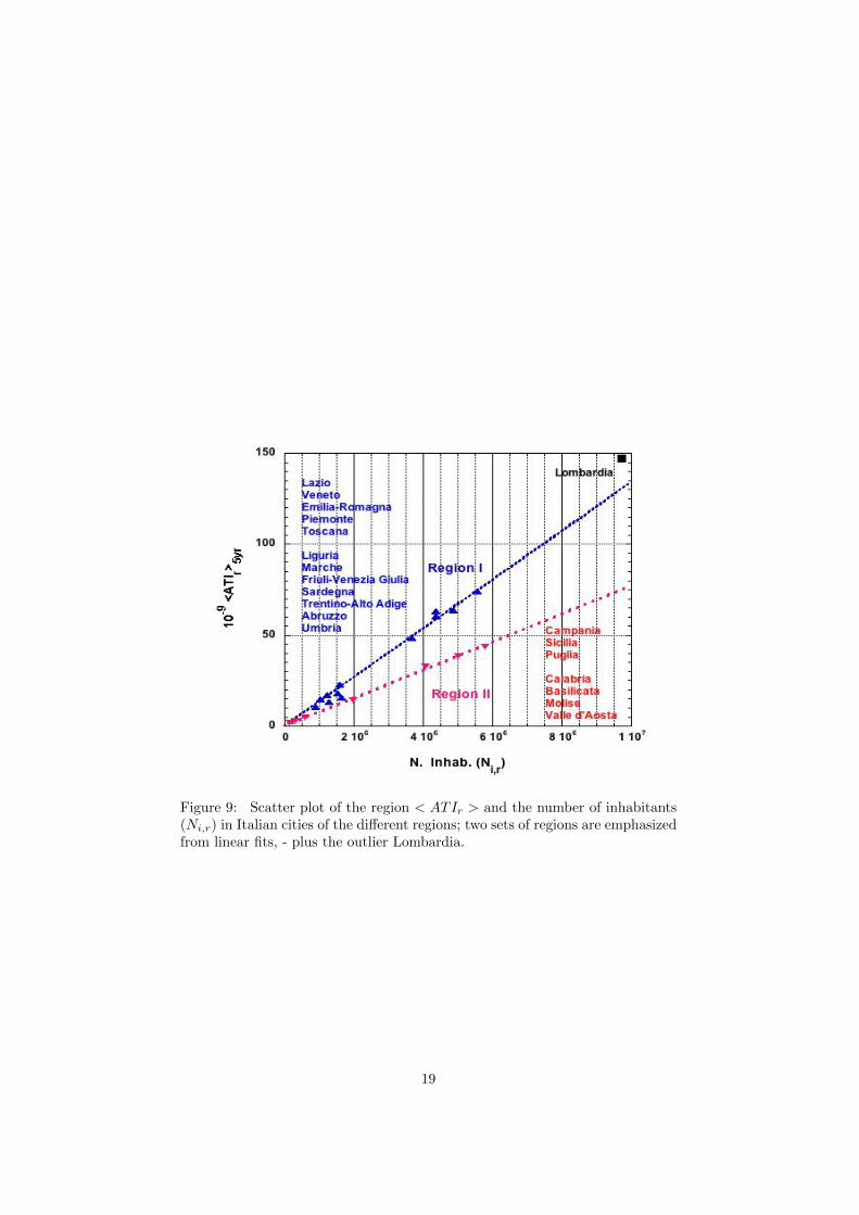
Figure 9: Scatter plot of the region < ATIr > and the number of inhabitants(Ni,r) in Italian cities of the different regions; two sets of regions are emphasizedfrom linear fits, - plus the outlier Lombardia.
19

Figure 10: Scatter plot of the region rank for < ATI > with respect to thenumber of inhabitants in a region rank; sets of regions are emphasized by linearbest fits.
20

rNinhab ≤ r<ATI> is about 40%. This suggests a superposition of two homoge-neous/similar distributions.
It is also of interest to observe the scatter plot of the < ATI > (averagedfor the examined quinquennium) and the number of inhabitants in all Italiancities; this is shown in Fig. 6. Some structure inside the cloud of data pointscan be emphasized: two sets of cities seem existing. This is finely shown byvisually distinguishing two sets of data points, and subsequent linear fits: onehas (i) (blue dash line) y = 16 791.15 x, and (ii) (red dot line) y = 9 311.28x. An overall fit gives the proportionality (iii) (black continuous line) y = 15942.30 x. The fits cannot be compared through their regression coefficient; theyare all close to 0.96, but we emphasize that the visual inspection leads to someevidence. Notice that (i) Milano appears to be an outlier; (ii) the red dot lineseems to point to a set of cities ”from the South”; (iii) in contrast to the bluedash line, pointing cities ”from the North”.
The scatter plot of the number of inhabitants and the < ATI > is alsopresented in Fig. 7, but on a log-log scale. This allows to emphasize the lowvalues. The two different regimes are not well seen. It is like Fig. 6 with achange in x and y axes. A power law fit through the cloud leads to the maininertia axis equation given by y ' 0.456 10−3 x0.915, with a regression coefficientR2 = 0.963.
Let us now again take two focussing points: (i) the cities in the whole countryand (ii) the regions.
Recall that the regions having a change over the quinquennium in the numberof cities are indicated by an arrow ↑ or ↓; the arrow direction is according tothe change in Nc,r in some year as mentioned in Table 1. The fit in Fig. 1captures the administrative changes. It is based on the function in Eq. (3.1);the fit parameters are given in the text. Administrative changes are usually dueto local tensions grounded on historical motivations. Discussing such aspects isfar beyond the scopes of this paper. However, it is important to note that thedefinition of the bounds of the IT regions derive often from the administrativestructure of Kingdoms and States in the Italian territory after the Holy RomanEmpire. In this respect, the influence of the historical facts occurred in Italy(Napoleon, the evolution of the Papacy, etc.) played also a relevant role.
Rank plots can be produced on classical, semi-log or log-log axes. In the firstcase, the data looks like a mere decaying convex function. However on semi-log (Fig. 2) and on log-log (Fig. 4), the ATI (and usually other data) showssome structure. An inflection point is well seen near rM/2 ∼ 4000, on the2007-2011 yearly ATI of the 8902 IT cities ranked according to their ”incometax” importance (Fig. 2). Some jumps between r = 7 and r = 8 are wellmarked on the log-log plot (Fig. 4). The rank plots are particularly meaningfulin describing the economical structure of Italy under the point of view of themunicipalities. The widest part of Italian cities has comparable small amountof ATI; this explains the inflection point at rM ∼ 4000 and why the yearlyATI decreases vertically with the rank for rank high enough. The jumps in thehighest rank cities identifies the great differences among the cities with highestvalues of < ATI >. Such a difference is reduced for low ranked cities; this leadsto some understanding of the polarization of the aggregated (citizen) incomevalues in the main urban areas.
Such results are confirmed also by visually inspecting the semi-log plot ofthe rank-size relationship between each Italian city < ATI > (averaged for
21

the examined quinquennium) and its rank (Fig. 3). Some departure of thedata from the empirical fit can be noticed, mainly after the inflection point.Specifically, this happens for the cities ranked above r ' 6000, corresponding toan (averaged) ATI ∼ 107 . These 2000 or so cities contribute to ∼ 1.2 1010; meanµ ∼ 5.5 106; standard deviation σ ∼ 2.6 106 . Thus µ/σ ∼ 2.1 for these cities.These cities (roughly) correspond to those having less than 1000 inhabitants(the border rank is at 6154.5), and µ ∼ 543, σ ∼ 256; µ/σ ∼ 2.1 also. Suchnumbers are quite interesting, mainly if one notes that the total IT populationis about 5.957 107; µ ∼ 7361, σ ∼ 40262; µ/σ ∼ 0.183. Substantially, smallcities have a number of inhabitants which is, relatively to the mean, less volatilewhen compared to that of IT. This further confirms the polarization of Italianinhabitants in a small number of highly populated cities.
The demographic, ATI relationship displayed through the scatter plot of thecity ranks for < ATI >, in Fig. 5, indicates a rather huge variation. Howeverthe pair concordance is very high τ ' 0.849 and Z ' 114.6.
Interesting findings are seen in Fig. 6, for the scatter plot of the < ATI >(averaged for the examined quinquennium) and the number of inhabitants in allItalian cities. Two sets of cities are emphasized from linear fits. Such straightlines capture a relevant aspect of Italian reality, which is divided into differentincome distribution areas, the South being much poorer than the North. Thered dot line includes cities showing a low proportion between rank for < ATI >and rank for population. In the cities belonging to the blue dash line, such aproportion is high. Cities in the former case (Bari, Catania, Palermo, Napoli)are poorer than those of the latter one (Torino, Genova). Specifically, Torino isless populated and richer than Napoli (and, similarly, Genova is less populatedand with a higher ATI than Palermo). The reasons for this can be found inthe well-documented distortion of GDP due to illegal activities and organizedcrime, which is more pervasive in the South than in the North [67, 68, 69, 70].
The difference between the slopes of the red and blue lines in Fig. 5 maybe useful in providing a measure of the entity of shadow economy. Milanorepresents an outlier for a simple reason: even if it is not the political capital ofItaly (it is Rome), it is the financial one (the Italian Stock Market is in Milano).This explains the high value of ATI. Moreover, Milano has a highly populatedhinterland, with many big cities (like Sesto San Giovanni or Rho). Hence, it isthe center of a highly populated area, even though the municipality of Milanoitself is not excessively populated per se, i.e. with respect to its ATI value.
4.1 Regional disparities
Note for completeness, that the number of provinces in 2007, i.e. 103, has in-creased by 7 units (BT, CI, FM, MB, OG, OT, VS)5 to 110 provinces in 2011. Inthis time window, it is worth to point out that 228 municipalities have changedfrom a province to another one. Nevertheless, they remained in the same region,except for 7 cities from PU (the province of Pesaro and Urbino) in the Marcheregion, to RN (province of Rimini) in the Emilia Romagna region (Casteldelci,Maiolo, Novafeltria, Pennabilli, San Leo, Sant’ Agata Feltria, Talamello). Bylooking at the data, after calculating either the number (Ni,r) of inhabitants ina region or the regional ATI (ATIr), i.e. the sum for the relevant cities, in each
5e. g. see ISO code: http://en.wikipedia.org/wiki/Provinces of Italy.
22

year and the subsequent average, the change in regional membership appears tobe very weakly relevant.
Thus, the regions can be also ranked each year according to their Ni,r anddisplayed on a plot (Fig. 8), corresponding to Nc,r in Fig. 1. Similarly, theregions can be ranked according to their yearly ATIr. For conciseness, this isshown on this same Fig. 8. The fit parameters to Eq. (3.1), with A pre-imposedto be = 109, are respectively m1 = 0.445 10−3; m2 = 0.287; m3 = 1.006 withR2 = 0.954 for Ni,r, and m1 = 16.20; m2 = 0.54; m3 = 0.719, with R2 = 0.966for < ATIr >.
It should not be necessary to repeat that the rank of a region is not the samewhen ranking the < ATIr > (averaged for the examined quinquennium) andwhen considering the number of inhabitants Ni,r. The comparison of the regionrespective ranks is however quite illuminating: first, the Kendall τ calculationcan be easily performed; results are given in Table 4, column (ii). The τ andρ values are large (τ ∼ 0.78, ρ ∼ 0.9098), but they are smaller than when notdistinguishing regions.
Remarkably, the data and fits (to the function in Eq. (3.1)) for Ni,r in ITregions and averaged regional ATI vs. the rank of the region for the years of thequinquennium in Fig. 8 indicate a coherence with respect to Fig. 1, althoughthe data transformation is not that trivial. This shows again that a rank-sizerule is of great interest, showing structures not seen when absolute value-sizerelations are displayed or analyzed.
This is emphasized in the scatter plot of the region < ATIr > (averaged forthe examined quinquennium) and the number of inhabitants (Ni,r) as well asthe classical scatter plots in Italian cities of the different regions; Fig. 9 andFig. 10. Remarkably, it is visually found that IT regions belong to differenttypes of sets. These sets of regions can be emphasized also through linear fits:(i) a classical scatter plot points to three sets of regions, beside the outlier(Lombardia). Furthermore, the scatter plot of ranks indicate the existence ofsubregions. Those sets are characterized by a ratio between the ATI and thenumber of inhabitants, either greater or smaller than an ”equilibrium point”.
Fig. 9 provides a regional confirmation of the analysis carried out at themunicipality level. The poor regions are the Southern ones, while the cities inthe North are those belonging to the qualified group of high ATI. Valle d’Aostaand Sardegna are peculiar cases of wrong classes (Valle d’Aosta is a rich regionbelonging to the South group, for Sardegna the converse applies). These findingsappear to us not so meaningful, being Valle d’Aosta and Sardegna positionedat the origin of the Cartesian plan in Fig. 9. As for the cities, Milano is anoutlier; for regions, Lombardia plays a similar outlier role. These outcomesdescribe well the situation of highly productive regions in the North of Italy,with a South affected by the organized crime and poor government institutionsdistorting economical resources.
Also in this case, the gap between the slopes of the blue and the red linesmay provide a good idea on how the ratio between population and aggregatedtax income should be (blue line, the North), but how it is presently in the South(red line).
The rank-rank scatter plot of the region rank for < ATI > (averaged forthe examined quinquennium) with respect to the number of inhabitants in aregion rank, Fig. 10, is very interesting, and fits well with results obtained bythe reading of Fig. 9. Regions are confirmed to be clustered in two groups (sets
23

of regions are emphasized by linear best fits). This is in agreement with thebrief discussion here above on the Italian socio-economic differences betweenthe Northern regions and the Southern ones.
To conclude, it is worth noting the high variance, positive skewness andkurtosis of the distributions of ATI (see Table 2.). Observe also the µ/σ valuesand time evolution in this Table 2 : an increase in this variable indicates a sortof tendency to peaking of the sample distribution. Nevertheless, its small valueindicates a quite large variety in intrinsic ATI values for the various cities. Thiseffect is much obscured when looking at the regional level, since then µ/σ '1.12.
5 Model
A specific modeling is presented based on arguments derived from statistics.First of all, it may be a wonder why a form like Eq. (3.1) is used. Observe
that it can be related to a power law with exponential cut-off [71], e.g., to theYule-Simon distribution [72, 17]
y(r) = h r−α e−λr, (5.1)
appropriately describing settlement formation (following the classical Yule model[72]) and its subsequent geographical distribution.
However, due to the finite size of the number N of data points, - therecannot reasonably be an infinite amount of cities in a region, the upper r regimeshould be considered as rather collapsing at the highest rank rM ≡ N . Thischaracterizes a function with an inflection point: for such a case, the Yule-Simondistribution can be adapted, bearing upon the fact that h e−λr ≡ d eλ(rM−r),and
eλ(rM−r) ' 1 + λ(rM − r) ' [1 + (rM − r)]λ (5.2)
for r → rM , thereby leading Eq. (5.1) to be written in the new form, that ofEq. (3.1),
y(r) = κ3(N r)−γ
(N − r + 1)−ξ(5.3)
The parameter κ3 (or m1 in Eq. (3.1)), is like the average amplitude of thedata, see h in Eq. (5.1) also. Some meaning of the exponent γ of the hyperbola,(or m2 in Eq. (3.1)), can be obtained from the decay exponent α in Eq. (5.1).Similarly, ξ (or m3 in Eq. (3.1)), has the meaning of the decay exponent of anorder parameter at a phase transition [73, 74, 75, 76]
Usually, the parameters (exponents), like m2 ↔ γ and m3 ↔ ξ, designate thestatistical physics model nowadays used for interpreting properties of a complexsystem, e.g. through phase transitions studies.
Having such ideas in mind, we suggest how to interpret the (m2 ↔ γ andm3 ↔ ξ) parameters through mathematical statistics theories, i.e. the incom-plete Beta function, as follows.
Recall that a preferential attachment process is an urn process in whichadditional balls (e.g, settlement locations) are added continuously to the systemand are distributed among the urns (e.g., areas) as an increasing function of thenumber of balls the urns already have. In the most general form of the process,
24
balls are added to the system at an overall rate of m new species for each newurn. This leads to the so called Yule-Simon probability distribution
f(a; b) = bB(a; b+ 1). (5.4)
where B(x; y) is the Euler Beta function
B(x; y) =Γ(x)Γ(y)
Γ(x+ y), (5.5)
Γ(x) being the standard Gamma function [77, 78].In practical words, a newly created urn (= region) starts out with k0 balls (=
cities) and further balls are added to urns at a rate proportional to the numberk that they already have plus a constant a ≥ −k0. With these definitions, thefraction P (k) of urns (areas) having k balls (cities) in the limit of long time isgiven by
P (k) =B(k + a; b)
B(k0 + a; b− 1)(5.6)
for k ≥ 0 (and zero otherwise). In such a limit, the preferential attachmentprocess generates a ”long-tailed” distribution following a hyperbolic (Pareto)distribution, i.e. power law, (∼ r−α or ∼ r−γ).
Moreover, a two-parameter generalization of the original Yule-Simon distri-bution replaces the Beta function with the incomplete Beta function:
Bε(a, b) =
∫ ε
0
xa (1− x)b dx (5.7)
In statistics, the expression xa(1 − x)b describes the probability of randomlyselecting a+ b real numbers in [0,1] such that the first a are in [0, x] and the last
b are in [x, 1]. The integral∫ 1
0xa (1 − x)b dx then describes the probability of
randomly selecting a + b + 1 real numbers such that the first number is x, thenext a numbers are in [0, x], and the next b numbers are in [x, 1].
It is worth noting that, in most of the studied examples concerning appli-cations of the Beta-function in statistical physics, the number of urns increasescontinuously, although this is not a necessary condition for a ”preferential at-tachment”. In fact, it is unconceivable that an infinite number of urns regions)can be created. Moreover, an increase in the number of settlements (cities) islimited by ”available resources”, e.g. by the socio-economic need for optimizingthe useful distances between settlements.
The product of two terms in Eq. (3.1) and the above reasoning remind ofthe Verhulst’s modification [79] of the Keynes population expansion equation,when introducing a ”capacity factor” .
6 Conclusions
This paper applies ideas of statistical mechanics in order to deal with an analysisof cities and regions. Specifically, the demographic (number of inhabitants, fromCensus 2011 - ISTAT) and the economic (ATI, averaged over the quinquennium2007-2011, from MEF) ranking are compared and discussed for Italian cities.
25

Two statistical physics-like instruments have been mainly employed: (i) a(new) rank-size rule found as a doubly decreasing power law type (see Eq.(3.1)and (ii) the computation of the Kendall τ and Spearman ρ coefficients for findingfluctuation correlations, and phase state discrimination.
• It is found that both cities and regions, within the country, can be clusteredin two categories, which mirror the Italian reality of a rich North anda poor South. Milano (city) and Lombardia (region) represent outliers,and cannot be indeed properly inserted in the resulting clusters. Somesocial, economical and political arguments might be carried out to explainthese findings. A few sentences have been introduced to suggest reasoningoutside the scope of this paper. It has seemed ppropriate to propose astatistical physics-like model, based on a number of evolving urn filling.
• Moreover, the above considerations and findings also serve as a demon-stration of the advantage and interest of the Kendall τ and Spearman ρcoefficients to analyze and understand various (equal size) lists of vari-ables measured according to various criteria. It has been pointed out thatsuch a measure is similar to the fluctuation correlation coefficient in thelinear response theory of statistical physics. Interestingly, it provided anindication of phase structures in the ”sample” (=country).
• For completeness, the Pearson Π coefficient has been calculated. It hasbeen argued that when the measurements are of so different natures, con-tain debatable error bars, rank-rank correlations are more meaningful, incontrast to the corresponding linear response theory coefficients in con-densed matter physics.
It is worth saying, in concluding, that the analysis at a provincial levelmight be of interest, but this leads to complications in the data and subsequentanalysis. The impact of the creation of new provinces (103 → 110) in theconsidered time period might be interesting, - such an administrative act, similarto the application of an external field, providing an extra axis for investigations.
Acknowledgements This paper is part of scientific activities in COSTAction IS1104, ”The EU in the new complex geography of economic systems:models, tools and policy evaluation”.
Appendix A. On data reorganization
During the examined time interval, several cities have merged into new ones,other were phagocytized. For completeness and thereby explaining some ”final-ized data reorganization”, we give here below the various cases ”of interest”.We use official IT acronyms for the regions:
(i) Campolongo al Torre (UD) and Tapogliano (UD) have merged after apublic consultation, held on Novembre 27th, 2007, into Campolongo Ta-pogliano (UD); thus 2 cities → 1 city only;
(ii) Ledro (TN) was the result of the merging (after a public consultation, heldon Novembre 30th, 2008) of Bezzecca (TN), Concei (TN), Molina di Ledro
26

(TN), Pieve di Ledro (TN), Tiarno di Sopra (TN) and Tiarno di Sotto(TN) as far as it is explained e.g. in http : //www.tuttitalia.it/trentino−alto− adige/18− concei/; thus 6 → 1;
(iii) Comano Terme (TN) results from the merging of Bleggio Inferiore (TN)and Lomaso (TN), in force of a regional law of November 13th, 2009; thus2 → 1;
(iv) Consiglio di Rumo (CO) and Germasino (CO) were annexed by Grave-dona (CO) on May 16th, 2011 and February 10th, 2011, to form the newmunicipality of Gravedona ed Uniti (CO); thus 3 → 1.
To sum up: 13 cities (in 2007) → 4 cities (in 2011). Thus, the number 8092taken as our reference number of municipalities in the main text.
Appendix B. A short note on time dependence
In this Appendix, it is verified that we do not bias the analysis when we takethe average of the ATI over the five year interval. In order to verify the point,we have examined the ATI year-year Kendall τ correlations with respect to eachother as well as with respect to the average6. From [65] the τ , Eq. (3.2), and Z,Eq. (3.3), values are easily obtained; the results are given in Table 5 and Table6. As mentioned in the main text, variations do exist but are rather mild.
Furthermore, a bonus is obtained in doing this time dependence examina-tion. The relevant quantities given in Tables 5-6 readily indicate a rather stablesystem of city hierarchies within the examined time interval; e.g. q/p ' 0.01.
Scatter plots for every pair and for the scatter plots of pair of ranks areavailable from the authors upon request.
Appendix C. Pearson coefficient
The Pearson Π coefficient, Eq.(3.4), is classically used to estimate a correlationbetween (supposedly normally distributed) sets of measures [80]. The Π valuesfor the case of the 8092 cities and the 20 regions, i.e. the value correlationsbetween the number of inhabitants (according to the 2011 Census) and thecorresponding averaged ATI (over the period 2007-2011) are given in Table 4.Values are in the same range as those of the Spearman ρ, but again much differfrom those of the Kendall τ . It can be briefly argued that this arises from thefact that the measurements are of different natures and found in intervals with aquite often unknown error bar, - like many econo-sociological surveys: there arenot even similar orders of magnitudes in measurements; there are outliers; theunits are wholly different ones. Moreover, for calculating a Pearson Π coefficient,and deducing its meaning, the measurements should conform to some normalitycriterion; this is not quite the case here. Figures 11-12 and Fig. 13 show thatthere are outliers and the measurements are not normality distributed.
In fact, rankings are thought to be more illuminating and appealing, themore so when there is a sort of ”competition”. As a case surely already met
6A Spearman ρ has not been computed in such cases; it is not expected to provide furtherinsights. Indeed, Spearman ρ is usually larger than Kendall τ ; τ is already remarkably largeas seen in Table 6.
27

Figure 11: Distribution of normalized quantiles for x, i.e., the average ATI forcities throughout the 20 IT regions.
by all readers, consider a hiring process in academia or a grant funding schemeto research groups: the hiring is strictly based on some ranking (and commit-tee member consensus, of course or through some vote procedure); the fundingis usually not based on the quantitative or qualitative values of groups (theyare usually measured through different indicators, like for the case in our text),relative to each other. All conclusions mainly depend on some ranking correla-tions through the chosen indicators. One (in fine) does not compare qualities.What is used is the rank. The measured quality has (alas) been by-passed. APearson correlation coefficient is rather irrelevant. The same is true in other”competitions”, like in sport. The gap in points, the quality or value, at thened of a ”season”, is masked by the ranking, when one wants to glorify a teamor an agent. This goes also in many other cases. Recently, Raschke et al. [81]have also concluded that the rank correlation is a more robust measure, in thefield of complex networks. This is exactly what we claim for the present case,but which is not per se a network.
References
[1] G.K. Zipf, Human Behavior and the Principle of Least Effort : An Intro-duction to Human Ecology (Addison Wesley, Cambridge, Mass., 1949).
28

Figure 12: Distribution of normalized quantiles for y, i.e. the number of inhab-itants in cities throughout the 20 IT regions.
q \ p 2007 2008 2009 2010 2011 < 5yav >2007 - 32322584 32191636 32162292 32128014 322941072008 413602 - 32476840 32430158 32381578 325614552009 544550 259346 - 32544918 32466870 325816892010 573894 306028 191268 - 32530208 325721912011 608172 354608 269316 205978 - 32521347
< 5yav > 442079 174731 154497 163995 214839 -
Table 5: The number of concordant pairs p (above the diagonal) and that ofnon-concordant pairs q (below the diagonal) of the 8092 cities, according totheir ATI value, for every year pairs.
29

Figure 13: Relationship and distribution of the number of inhabitants and theaverage ATI in corresponding IT regions.
Z \ τ 2007 2008 2009 2010 2011 < 5yav >2007 - 0.9747 0.9667 0.9649 0.9628 0.97302008 131.49 - 0.9842 0.9813 0.9783 0.98932009 130.42 132.77 - 0.9883 0.9835 0.99062010 130.18 132.38 133.32 - 0.9874 0.99002011 129.89 131.98 132.68 133.21 - 0.9869
< 5yav > 131.26 133.47 133.63 133.55 133.13 -
Table 6: Rank correlation test of the 8092 cities, according to their ATI value:τ (above the diagonal), Eq. (3.2), and Z (below the diagonal), Eq. (3.3), forevery year pairs.
30

[2] Newman M. E. J. (2005). Power laws, Pareto distributions and Zipf’s law.Contemporary Physics, 46, 323 - 351.
[3] M. Jefferson, Geogr. Rev. 29, 226 (1939).
[4] M. Beckmann, Economic Development and Cultural Change 6, 243 (1958).
[5] X. Gabaix, Q. Econ. 114, 739 (1999); Am. Econ. Rev. 89, 129 (1999).
[6] L.M.A. Bettencourt, J. Lobo, G.B. West, Eur. Phys. J. B 63, 285 (2008).
[7] F. Semboloni, Eur. Phys. J. B 63, 295 (2008).
[8] P. Krugman, Geography and Trade (The MIT Press, Cambridge MA, 1991).
[9] B.J.L. Berry, Economic Development and Cultural Change 9, 573 (1961).
[10] S. Pianegonda, J.R. Iglesias, Physica A: Statistical Mechanics and its Ap-plications 342 193 (2004).
[11] G. Ottaviano, D. Puga, The World Economy 21, 707 (1998).
[12] M. Fujita, P. Krugman, and A.J. Venables, The Spatial Economics: Cities,Regions, and International Trade (The MIT Press, Cambridge, MA, 1999).
[13] J.P. Neary, Journal of Economic Literature 39, 536 (2001).
[14] R. Baldwin, R. Forslid, P. Martin, G. Ottaviano, F. Nicoud, Economicgeography and public policy. (Princeton University Press, Princeton, NJ,2003).
[15] M. Fujita, T. Mori. Papers in Regional Science 84, 377 (2005).
[16] B.K. Chakrabarti, A. Chakraborti, S.R. Chakravarty, A. Chatterjee,Econophysics of income and wealth distributions (Cambridge UniversityPress, 2013).
[17] N.K. Vitanov, Z.I. Dimitrova, Bulgarian Cities and the New EconomicGeography (Vanio Nedkov, Sofia, 2014).
[18] K.T. Rosen, M. Resnick, Journal of Urban Economics 8, 165 (1980).
[19] E.S. Mills, B.W. Hamilton, Urban Economics (Prentice Hall, 1994).
[20] F. Guerin-Pace, Urban Studies 32, 551 (1995).
[21] L.H. Dobkins, Y.M. Ioannides, Regional Science and Urban Economics31701 (2001).
[22] S. Song, K.H. Zhang, Urban Studies 392317 (2002).
[23] Y.M. Ioannides, H.G. Overman, Regional Science and Urban Economics33, 127 (2003).
[24] X. Gabaix, Y.M. Ioannides, The Evolution of City Size Distributions, in:Henderson, J.V., Thisse, J.-F. (Eds.), Handbook of Regional and UrbanEconomics, Vol. 4, (Elsevier, Amsterdam, 2004).
31

[25] W.J. Reed, Journal of Regional Science 42, 1 (2002),
[26] Z. Dimitrova, M. Ausloos, Primacy analysis of the system of Bulgariancities, arXiv : 1309.0079 (2013).
[27] E. Sheppard, Nonlinearities, Geographical Analysis 17, 47 (1985).
[28] R. Gibrat, Les inegalites economiques: Applications aux inegalites desrichesses, a la concentration des entreprises, aux populations des villes,aux statistiques des familles, etc., d’une loi nouvelle, la loi de l’effet pro-portionnel. (Sirey, Paris, 1931).
[29] V. Nitsch, Journal of Urban Economics 57 86 (2005).
[30] G. Peng, Physica A: Statistical Mechanics and its Applications 389, 3804(2010).
[31] Y.M. Ioannides, S.Skouras, Journal of Urban Economics 73, 18 (2013).
[32] V. J. Matlaba, M. J. Holmes, P.McCann, J. Poot, Review of Urban andRegional Development Studies 25, 129 (2013).
[33] K.T. Soo, Urban Studies 44, 1 (2007).
[34] J.-C. Cordoba, Urban Economics 63, 177 (2008).
[35] A.S. Garmestani, C.R. Allen, C.M. Gallagher, J.D. Mittelstaedt, UrbanStudies 44, 1997 (2007).
[36] M. Bosker, S. Brakman, H. Garretsen, M. Schramm, Regional Science andUrban Economics 38, 330 (2008).
[37] A.S. Garmestani, C.R. Allen, C.M. Gallagher, Journal of Economic Behav-ior and Organization 68, 209 (2008).
[38] R.K. Skipper, McNair Scholars Undergraduate Research Journal 3, 217(2011).
[39] M. Cristelli, M. Batty, L. Pietronero, Scientific Reports 2, 812 (2012).
[40] K. Giesen, J. Sudekum, Journal of Economic Geography 11, 667 (2011).
[41] M. Kendall, Biometrika 30,81 (1938).
[42] H. Abdi, The Kendall Rank Correlation Coefficient. In Neil Salkind (Ed.):Encyclopedia of Measurement and Statistics. (Sage, Thousand Oaks (CA),2007).
[43] C. Spearman, American Journal of Psychology 15, 201 (1904).
[44] S.-D. Bolboacaa, L. Jantschi, Leonardo Journal of Sciences 9, 179 (2006).
[45] M. Bland, An Introduction to Medical Statistics, Oxford University Press;Oxford, New York, Tokyo, pp. 205-225, (1995).
[46] M. Melucci, SIGIR Forum 41, 18 (2007).
32

[47] M. Ausloos, Central European Journal of Physics 12, 773 (2014).
[48] M. Ausloos, R. Cloots, A. Gadomski, N.K. Vitanov, International Journalof Modern Physics C 25, 1450060 (2014).
[49] M. Ausloos, A. Gadomski, N.K. Vitanov, Phys. Scr. 89, 108002 (2014).
[50] T.S. Hare, The Archaeology of Communities: A New World Perspective ,78 ( 2000).
[51] Y.-B. Zhou, , L. Lu, M. Li, M., New Journal of Physics 14, 033033 (2012).
[52] M. Ausloos, Scientometrics 95, 895 (2013).
[53] J. Stallings, E Vance, J Yang, MW Vannier, J. Liang, L. Pang, L. dai, I. Ye,G. Wang, Proceedings of the National Academy of Science of the UnitedStates of America 110, 9680 (2013).
[54] J.-J. Hsieh Computational Statistics & Data Analysis 54(6), 1613-1621(2010).
[55] B. Yang, Y. Peng, H. Chi-Ming Leung, S.-M. Yiu, J.-C. Chen, F. Yuk-LunChin BMC Bioinformatics 11 (suppl. 2), S5, (2010).
[56] M. Rezapour, N. Balakrishnan Statistical Methodology 15, 55-72 (2013).
[57] R.J. Schmitz, M.D. Schultz, M.A. Urich, J.R. Nery, M. Pelizzola, O. Li-biger, A. Alix, R.B. McCosh, H. Chen, N.J. Schork, J.R. Ecker Nature 495,193198 (2013).
[58] J. Rappoport, Regional Science and Urban Economics 38, 533 (2008).
[59] T. Mori, T.E. Smith, Journal of Regional Science 51, 694 (2011).
[60] H.L.F. De Groot, J. Poot, M.J. Smit, Agglomeration, innovation andregional development: theoretical perspectives and meta-analysis. In: R.Capello and P. Nijkamp (eds), Handbook of regional growth and develop-ment theories (Edward Elgar, Cheltenham, 2009.) 256-281.
[61] P.C. Melo, D.J. Graham, R.B. Noland, Regional Science and Urban Eco-nomics 39, 332 (2009).
[62] M. Ausloos, J. Appl. Quant. Meth. 9, 1 (2014).
[63] R Kubo, Journal of the Physical Society of Japan 12, 570 (1957).
[64] R Kubo, Reports on Progress in Physics 29, 255 (1966).
[65] P. Wessa, Kendall τ Rank Correlation (v1.0.11) in Free Statistics Soft-ware (v1.1.23-r7), Office for Research Development and Education, http ://www.wessa.net/rwasp−kendall.wasp/(2012).
[66] D.G. Bonett, T.A. Wright , Psychometrika 65, 23 (2000).
[67] G Brosio, A Cassone, R Ricciuti, Public Choice 112, 259 (2002).
[68] C.V. Fiorio, F. D’Amuri, Giornale degli Economisti e Annali di Economia64, 247 (2005).
33

[69] F. Calderoni, Global Crime 12, 41 (2001).
[70] R. Galbiati, G. Zanella, Journal of Public Economics, 96, 485 (2012).
[71] C. Rose, D. Murray, D. Smith, Mathematical Statistics with Mathematica(Springer, New York, 2002), p. 107.
[72] G.U. Yule, Phil. Trans. Roy Soc. London B 213, 21 (1922).
[73] C.J. Thompson, Mathematical statistical mechanics (Macmillan, London,1971).
[74] H.E. Stanley, Phase transitions and critical phenomena (Clarendon Press,London. 1971).
[75] M.E. Fisher, Rev. Mod. Phys. 70, 653 (1998).
[76] H.E. Stanley, Rev. Mod. Phys. 71, 358 (1999).
[77] I.S. Gradshteyn, I.M. Ryzhik, Table of Integrals, Series and Products (Aca-demic Press, New York, 2000).
[78] M. Abramowitz, I. Stegun, Handbook of Mathematical Functions (Dover,New York, 1970)
[79] P.F. Verhulst, Nouveaux Memoires de l’Academie Royale des Sciences etBelles-Lettres de Bruxelles 18, 1 (1845).
[80] W. L. Hays, Statistics, (CBS College Publishing, New York, 1988).
[81] M. Raschke, M. Schlapfer, R. Nibali Phys. Rev. E 82, 037102 (2010),
34