CRLB via Automatic Differentiation: DESPOT2

Jul 12, 2013Jason Su

Overview

• Converting Matlab DESPOT simulation functions to Python and validation

• Extension of pyautodiff package to Jacobians• Application to CRLB in DESPOT1, DESPOT2,

and DESS• Other projects:– 7T Thalamus ROI analysis– 7T MS segmentation

Validation: SPGR & SSFP• Just a sanity check that I correctly ported the single-component

functions• 700 SPGR values are compared between Matlab and Python

– 10 T1s from 1000-2000ms, and 70 flip angles from 1-70deg• 14,000 SSFP values are compared each for before and after RF

excitation equations• All results are the same within machine accuracy

Validation: AD/FD vs Symbolic

A comparison between automatic and (central) finite differentiation vs. symbolic

AD matches symbolic to machine precision

Finite difference doesn’t come close

Extending pyautodiff with Jacobian

Many packages support derivatives of multi-output functions, i.e. Jacobian• pyautodiff is not one of them• I chose pyautodiff because it does not require usage of

special elementary functions, it can analyze code with no modification• Leverages a project called “theano” which can

optimize by Python by dynamically creating C code• Instead, analyzes function inputs and output to

produce the graph for chain rule derivative calculation

Extending pyautodiff with Jacobian

I extended pyautodiff to do so. Ramifications:• The Jacobian of nearly any analytic and even programmatic

function with arbitrary number of inputs or outputs can be computed in 1 line• Not sure yet how to handle matrix inverse. There is support in

theano so I think pyautodiff should too but still need to try it.• Calculation of an entire space of Jacobians can be done with a

single call, e.g. a 4D space of T1s, T2s, phase cycles, and FAs• Maintained compatibility with NumPy broadcasting, no for loops• This makes it possible to explore an optimal protocol by

evaluating the CRLB over a space of relevant tissues

CRLB: Goals

• With these new tools, I set out to explore all forms of single-component DESPOT with the CRLB formalism

• Expected to see results as in Deoni 2004 “Determination of Optimal Angles…”– Also, if yes, then validates CRLB as a useful

criterion to find an optimal protocol because would then be an equivalent analysis

CRLB: Parameters

• TR = 5ms, M0 = 1, T1 = 50-5000ms (100pts)• σS = 2e-3 (SNR≈20 over mean of SPGR curve)

– The “ideal” protocol is scaled by sqrt(5) to match SNR of the others

• I use the protocols considered in Deoni 2004:spgr_angles = { 'tuned': np.array([2, 3, 4, 5, 6, 7, 8, 9, 10, 12]), 'ideal': np.array([3, 12]), 'ga': np.array([2, 3, 4, 5, 7, 9, 12, 14, 16, 18]), 'weighted ga': np.array([2, 3, 4, 5, 7, 9, 11, 14, 17, 22]),}

DESPOT1-SPGR: Constant Noise

CoV is how Lankford presents CRLB results at a given noise level

Deoni 2004 flips the scale to T1NR and normalizes it as a factor of the SNR at the Ernst angle (with equivalent NEX)

ESNRn

NRTH

11

Constant SNR: Converting to H1

• n=10, the equivalent NEX• mp/n is a scale factor that scales the noise down if less

flip angles are collected, e.g. mp=2 for “ideal” so variance reduces by 5x

1

1

2111

1

11

11,

estimator unbiased

111

1

iiTp

sT

pii

TT

s

E

T

s

E

T

E

JJn

m

I

n

mJJ

Sn

T

Sn

TE

SNRn

NRTH

s

Constant SNR: Converting to H1• Suppose we normalize such that σS = SE, SNRE = 1

– Scale noise to Ernst angle signal, i.e. it becomes a function of T1

• This is like effectively simulating with Σ = sqrt(mp)SEI

1

1

11

11

1

11

11

1

1

iiT

Ep

iiTp

E

T

s

E

T

iiTp

EiiTp

sT

Es

JJSm

TH

JJn

mSn

T

n

T

Sn

T

H

JJn

mSJJ

n

m

S

argmaxα(SPGR): Ernst Angle

2max

max

1/

11

110

1arccoscos11

sin1100

1

E

EMSS

EE

EM

eE

E

TTR

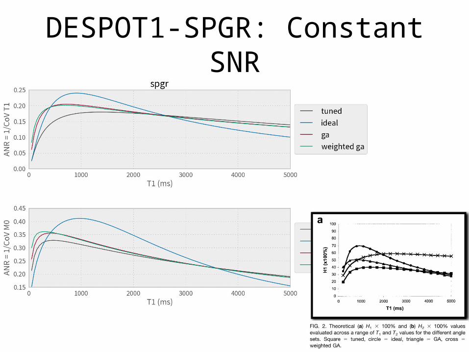
DESPOT1-SPGR: Constant SNR

Results

• Curve shapes are similar except for “weighted ga”– I’m not sure how to incorporate this with CRLB– Intuitively it would be to weight Σ, but the

interpretation would then equivalently be that the noise is changing with different angles• Does that make sense?

– Not exactly the same, note the intersection point• There is still a scaling difference though– Something different about H1 calculation?

Results

• Note how fundamentally different approaches arrive at a similar answer– Deoni 2004 approximates the solution to the curve fitting

cost function with a Taylor expansion– CRLB computes relationships based on the Jacobian of SPGR– Both involve squaring derivatives of SPGR, maybe not

surprising• I think the preliminary CRLB results with constant noise

is actually more realistic/useful– Noise is independent of tissue (or at least scanner noise

dominates)

CRLB: Parameters

• TR = 5ms, M0 = 1, T1 = 50-5000ms (100pts), T2 = 10-200ms (50pts)• Protocols:

despot2_angles = { 'tuned': { 'spgr': np.array([2, 3, 4, 5, 6, 7, 8, 9, 10, 12]), 'ssfp_before': np.array([8, 12, 18, 24, 29, 36, 48, 61, 72, 83]), 'ssfp_after': np.array([8, 12, 18, 24, 29, 36, 48, 61, 72, 83]), }, 'ideal': { 'spgr': np.array([3, 12]), 'ssfp_before': np.array([20, 80]), 'ssfp_after': np.array([20, 80]), }, 'ga': { 'spgr': np.array([2, 3, 4, 5, 7, 9, 12, 14, 16, 18]), 'ssfp_before': np.array([8, 13, 19, 25, 37, 45, 58, 71, 81, 87]), 'ssfp_after': np.array([8, 13, 19, 25, 37, 45, 58, 71, 81, 87]), }, 'weighted ga': { 'spgr': np.array([2, 3, 4, 5, 7, 9, 11, 14, 17, 22]), 'ssfp_before': np.array([5, 10, 16, 24, 32, 43, 54, 66, 75, 88]), 'ssfp_after': np.array([5, 10, 16, 24, 32, 43, 54, 66, 75, 88]), },}

DESPOT2-SSFP

• T1 is assumed from DEPOT1 and those rows/columns eliminated from JbSSFP

argmaxα(bSSFP): “bErnst”

• For simplification, I set phase π– Mx = 0 in this case– Recall the observation that the max signal is constant over phase– I start with the post-RF equations from Freeman-Hill, which

differ from those in Deoni 2009 (pre-RF)

211

21arccos

221cos1cos1121

sin211100

2,1

max

2/1/

EE

EE

EEEEE

EEM

eEeE TTRTTR

DESPOT2: Constant SNR – Tuned

DESPOT2: Constant SNR – Ideal

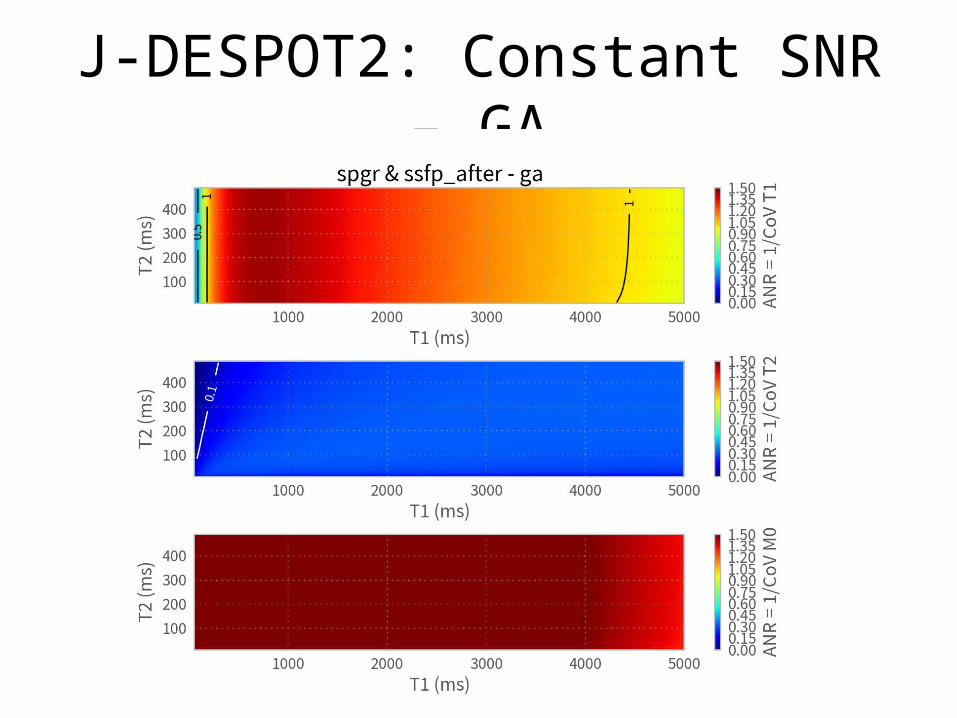
DESPOT2: Constant SNR – GA

DESPOT2: Constant SNR – Wtd GA

Results

• Take Weighted GA with a grain of salt as it may not be correct as we saw with SPGR

• Ideal has focused itself with a smaller cone of high T2NR• GA has the most uniform T2NR as expected

• As a side note, we can include T1 in J and try to evaluate the precision of bSSFP to estimate all 3 parameters– F (Fisher Information Matrix) is then ill-conditioned, a known

property that SSFP can’t do everything by itself

Joint DESPOT2

• Next I perform the analysis assuming a joint fit of T1, T2, and M0 with both the SPGR and bSSFP equations

• The noise normalization is increased by sqrt(2) to account for the doubling of total images collected

J-DESPOT2: Constant SNR – Tuned

J-DESPOT2: Constant SNR – Ideal

J-DESPOT2: Constant SNR – GA

Results

• Interpretation of the scale is not intuitive?– Mixed sequences but each is normalized to have peak

SNR of 1 at Ernst/bErnst– Does it make sense that estimate of T1 or M0 can be

better than peak SNR of underlying images?

• With a joint fit, the tuned set appears to trade more uniform T1NR for a small price in T2NR– GA isn’t a clear winner here, but may be if we only

care about a certain range

Joint DESSPOT2

• Next I perform the analysis assuming a joint fit of T1, T2, and M0 with both the SPGR and dual-echo SSFP equations– I model DESS as the magnetization before and after

RF excitation, equations from Freeman-Hill 1971

• TR is kept the same and the same flip angle protocols are examined

• Noise is now scaled up by sqrt(3)

J-DESSPOT2: Constant SNR – Tuned

J-DESSPOT2: Constant SNR – Ideal

J-DESSPOT2: Constant SNR – GA

Results• Perhaps unsurprisingly, we lose some T1NR

– Since SPGRs have more noise• But we gain some T2NR• Interestingly, tuned protocol splits into 2 cones for T2 estimation

T1-Mean T1-Std T2-Mean T2-Std M0-Mean M0-Std

tuned J-DESPOT2 1.127 0.175 0.283 0.062 1.831 0.305J-DESSPOT2 0.927 0.144 0.339 0.073 1.508 0.248

ideal J-DESPOT2 1.177 0.342 0.290 0.046 2.050 0.602J-DESSPOT2 0.967 0.278 0.345 0.053 1.686 0.489

ga J-DESPOT2 1.191 0.181 0.294 0.056 1.889 0.374J-DESSPOT2 0.978 0.147 0.350 0.063 1.554 0.304

wtd ga J-DESPOT2 1.186 0.166 0.286 0.057 1.892 0.384J-DESSPOT2 0.974 0.134 0.341 0.065 1.556 0.312

bSSFP• Plots show signal curves at

different θ• Mx is symmetric about θ=π (0.5

cycles here)• My has a crossover point where

all phase curves intersect– Its x,y location is defined by E1

and E2

• Magnitude max over flip angle is constant with phase

• Phase is constant with phase– Can we use this to get off-

resonance?

Next Steps• CRLB with real/imag or mag/phase?• DESPOT2-FM

– Analysis, visualization will be trickier as want to see precision as a function of off-resonance too• Estimation of M0, T1, T2, θ as a function of T1, T2, θ

– Protocol optimization, including TR

• A protocol that optimizes precision in B1 inhomogeneity? Assuming B1 map is known

– Maximize ∫T1NR(κ)dκ for a given (or range of) T1

• mcDESPOT– Protocol optimization– Exploration of DESS and other sequences

7T MS: PVF Pipeline

• Goal is to compute atrophy by generating 2 masks reliably:– Intracranial mask– Parenchyma mask

• In MSmcDESPOT we did:– Intracranial mask = BET mask on T1w, includes ventricles but

generally excludes space between brain and skull -> not exactly what is stated

– Parenchyma mask = WM+GM, essentially excludes ventricle CSF

7T MS: PVF Pipeline

New pipeline uses both T1w and T2w:

• Intracranial mask = BET mask on T2w, includes cortical CSF, then manually edit to only keep supratentorial brain

• Brain mask = segment CSF with SPM8 and subtract• We also remove everything outside BET mask on

registered T1wSince CSF is dark on T1w, this is another way to cut out cortical CSF and any other stray matter outside brain

• Requires some special handling to deal with 7T inhomogeneity (bump up the bias correction by 100x)

Future Segmentation

Natalie suggested some ideas to attempt automatic segmentation via registration

• 1st we should try with simple tasks like the removal of cerebellum done in the intracranial mask editing

I probably want to finally learn nipype for this as it sounds like it will require integration of many packages:

• ANTS for study-specific template to register to• ITK to do the nonlinear registration (Natalie said this is faster/better for binary masks where

we care about the outside contour and not the inside)• FSL and NumPy for generating masks to restrict the registration to ROI

Hope to extend it to whole thalamus and hippocampus, nuclei would probably be in our dreams

Lesions

• Waiting for normal population to perform standard space z-score thresholding on FLAIR as in MSmcDESPOT

• Hopefully registration is not too problematic with 7T data

7T Thalamus

• Used gaussian KDE to approximate distribution– Width of kernel is automatically determined by the

function

7T Thalamus

• In the future, I imagine we want to do ANOVA testing of T1 values between all the ROIs– Or some non-parametric variant (Kruskall-Wallis I

think)– We can then multiply that elementwise by an

“adjacency matrix” that flags which nuclei are neighbors• Gives us which nuclei are separable from each other if

we take their spatial location into account