Applications of Automatic Differentiation and the Cramér-Rao Lower Bound to Parameter Mapping

July 31, 2013Jason Su

Outline

Background and Tools• Cramér-Rao Lower Bound (CRLB)• Automatic Differentiation (AD)

Applications in Parameter Mapping• Evaluating methods• Protocol optimization

Cramér-Rao Lower Bound

How precisely can I measure something with this pulse sequence?

CRLB: What is it?

• A lower limit on the variance of an estimator of a parameter.– The best you can do at estimating say T1 with a given pulse

sequence and signal equation: g(T1)

• Estimators that achieve the bound are called “efficient”– The minimum variance unbiased

estimator (MVUE) is efficient

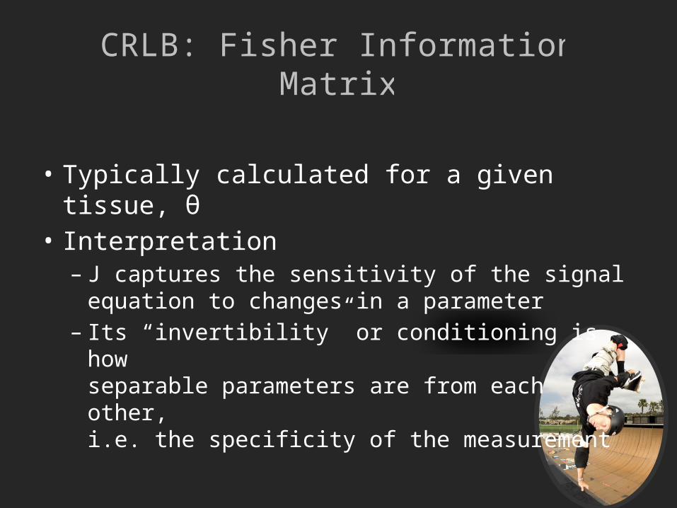
CRLB: Fisher Information Matrix

• Typically calculated for a given tissue, θ• Interpretation– J captures the sensitivity of the signal equation to

changes in a parameter– Its “invertibility” or conditioning is how

separable parameters are from each other,i.e. the specificity of the measurement

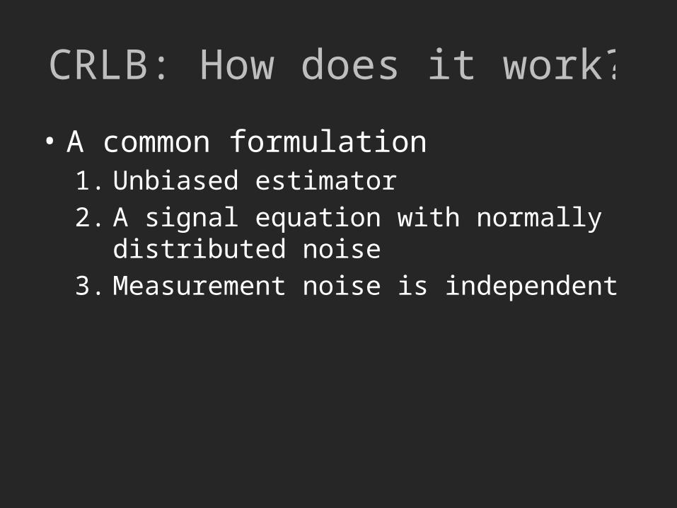
CRLB: How does it work?

• A common formulation1. Unbiased estimator2. A signal equation with normally distributed noise3. Measurement noise is independent

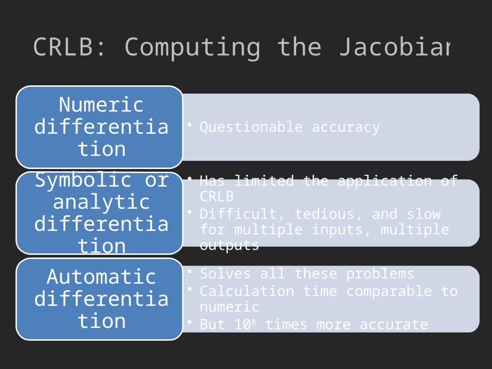
CRLB: Computing the Jacobian

• Questionable accuracyNumeric differentiation

• Has limited the application of CRLB• Difficult, tedious, and slow for multiple inputs,

multiple outputs

Symbolic or analytic

differentiation

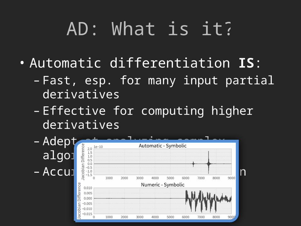
• Solves all these problems• Calculation time comparable to numeric• But 108 times more accurate

Automatic differentiation

Automatic Differentiation

The most criminally underused tool in your computational

toolbox?

AD: What is it?

• Automatic differentiation is NOT:– Analytic differentiation

𝑓 (𝑥1 , 𝑥2 )= 1

1+𝑒−𝑥1𝑥2

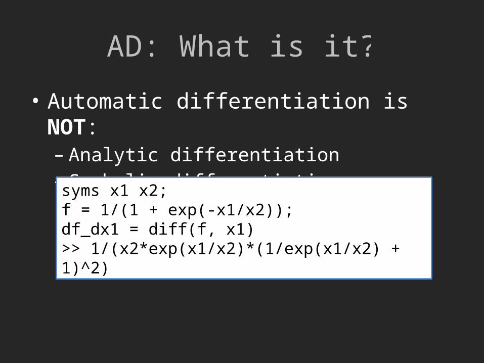
AD: What is it?

• Automatic differentiation is NOT:– Analytic differentiation– Symbolic differentiation

syms x1 x2;f = 1/(1 + exp(-x1/x2));df_dx1 = diff(f, x1)>> 1/(x2*exp(x1/x2)*(1/exp(x1/x2) + 1)^2)

AD: What is it?

• Automatic differentiation is NOT:– Analytic differentiation– Symbolic differentiation– Numeric differentiation (finite difference)

f = @(x1, x2) 1/(1 + exp(-x1/x2));eps = 1e-10;df_dx1 = f(x1+eps, x2) – f(x1, x2))df_dx1 = df_dx1/eps

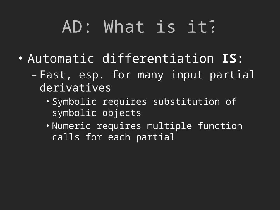
AD: What is it?

• Automatic differentiation IS:– Fast, esp. for many input partial derivatives• Symbolic requires substitution of symbolic objects• Numeric requires multiple function calls for each partial

AD: What is it?

• Automatic differentiation IS:– Fast, esp. for many input partial derivatives– Effective for computing higher derivatives• Symbolic generates huge expressions• Numeric becomes even more inaccurate

AD: What is it?

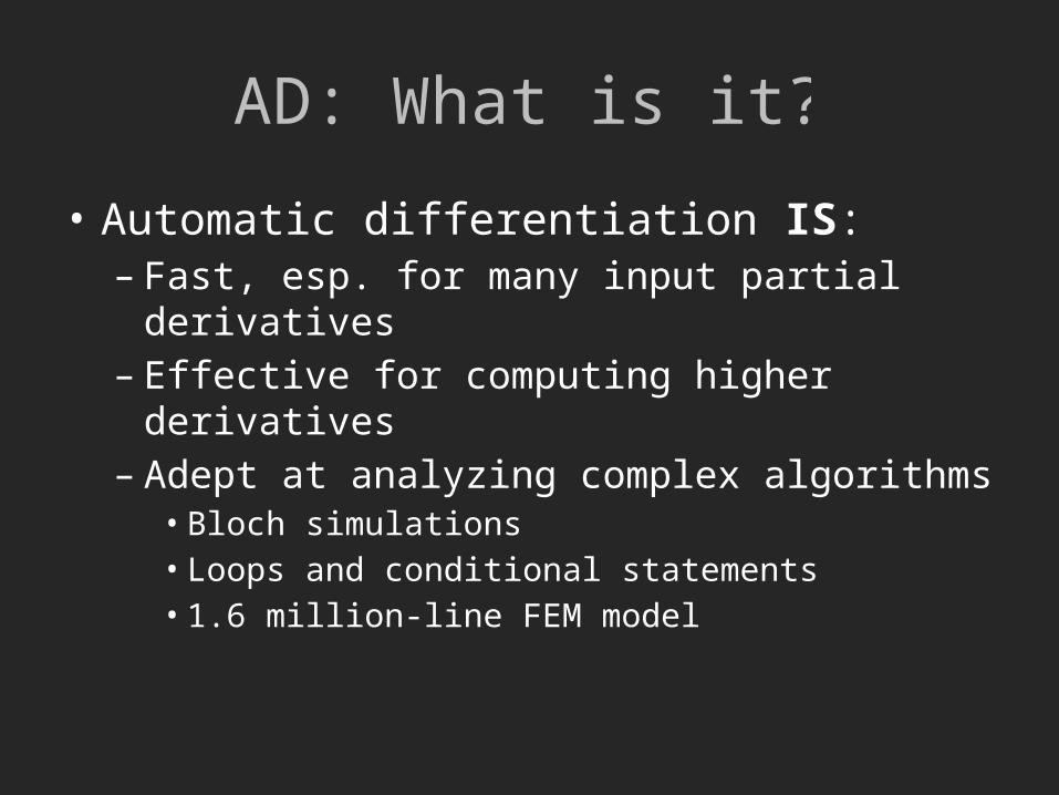
• Automatic differentiation IS:– Fast, esp. for many input partial derivatives– Effective for computing higher derivatives– Adept at analyzing complex algorithms• Bloch simulations• Loops and conditional statements• 1.6 million-line FEM model

AD: What is it?

• Automatic differentiation IS:– Fast, esp. for many input partial derivatives– Effective for computing higher derivatives– Adept at analyzing complex algorithms– Accurate to machine precision

AD: What is it?

• Some disadvantages:– Exact details of the implementation are hidden– Hard to accelerate

AD: How does it work?

• Numeric: implement definition of derivative• Symbolic: N-line function -> single line

expression

• Automatic: N-line function -> M-line function– A technology to automatically

augment programs with statements to compute derivatives

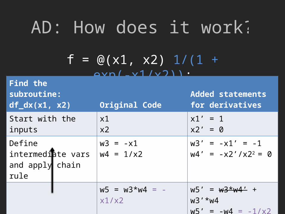
AD: How does it work?

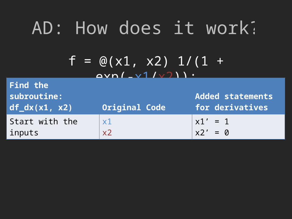
f = @(x1, x2) 1/(1 + exp(-x1/x2));

• Build a graph of intermediate quantities and apply the chain rule

AD: How does it work?

f = @(x1, x2) 1/(1 + exp(-x1/x2));Find the subroutine:

df_dx(x1, x2) Original CodeAdded statements for derivatives

Start with the inputs x1x2

x1’ = 1x2’ = 0

AD: How does it work?

f = @(x1, x2) 1/(1 + exp(-x1/x2));Find the subroutine:

df_dx(x1, x2) Original CodeAdded statements for derivatives

Start with the inputs x1x2

x1’ = 1x2’ = 0

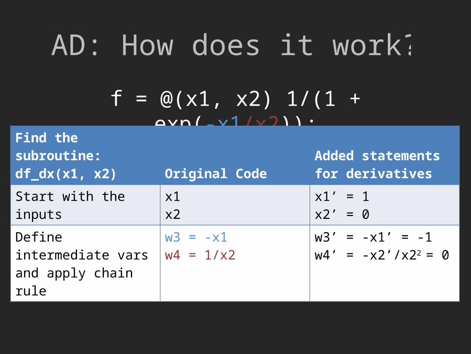
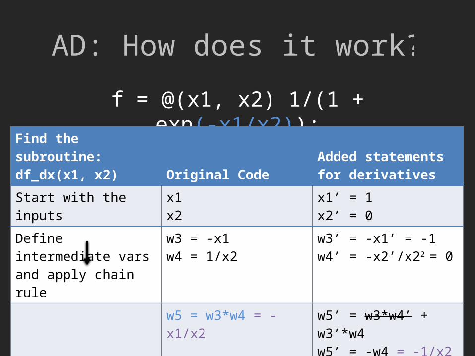
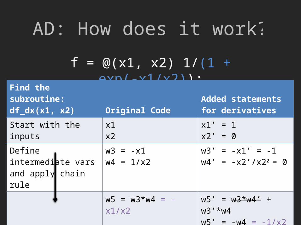
Define intermediate varsand apply chain rule

w3 = -x1w4 = 1/x2

w3’ = -x1’ = -1w4’ = -x2’/x22 = 0

AD: How does it work?

f = @(x1, x2) 1/(1 + exp(-x1/x2));Find the subroutine:

df_dx(x1, x2) Original CodeAdded statements for derivatives

Start with the inputs x1x2

x1’ = 1x2’ = 0

Define intermediate varsand apply chain rule

w3 = -x1w4 = 1/x2

w3’ = -x1’ = -1w4’ = -x2’/x22 = 0

w5 = w3*w4 = -x1/x2 w5’ = w3*w4’ + w3’*w4w5’ = -w4 = -1/x2

AD: How does it work?

f = @(x1, x2) 1/(1 + exp(-x1/x2));Find the subroutine:

df_dx(x1, x2) Original CodeAdded statements for derivatives

Start with the inputs x1x2

x1’ = 1x2’ = 0

Define intermediate varsand apply chain rule

w3 = -x1w4 = 1/x2

w3’ = -x1’ = -1w4’ = -x2’/x22 = 0

w5 = w3*w4 = -x1/x2 w5’ = w3*w4’ + w3’*w4w5’ = -w4 = -1/x2

w6 = 1 + exp(w5) w6’ = w5’*exp(w5)

w7 = 1/w6 w7’ = -w6’/w62

AD: How does it work?

f = @(x1, x2) 1/(1 + exp(-x1/x2));Find the subroutine:

df_dx(x1, x2) Original CodeAdded statements for derivatives

Start with the inputs x1x2

x1’ = 1x2’ = 0

Define intermediate varsand apply chain rule

w3 = -x1w4 = 1/x2

w3’ = -x1’ = -1w4’ = -x2’/x22 = 0

w5 = w3*w4 = -x1/x2 w5’ = w3*w4’ + w3’*w4w5’ = -w4 = -1/x2

w6 = 1 + exp(w5) w6’ = w5’*exp(w5)

w7 = 1/w6 w7’ = -w6’/w62

AD: How does it work?

f = @(x1, x2) 1/(1 + exp(-x1/x2));Find the subroutine:

df_dx(x1, x2) Original CodeAdded statements for derivatives

Start with the inputs x1x2

x1’ = 1x2’ = 0

Define intermediate varsand apply chain rule

w3 = -x1w4 = 1/x2

w3’ = -x1’ = -1w4’ = -x2’/x22 = 0

w5 = w3*w4 = -x1/x2 w5’ = w3*w4’ + w3’*w4w5’ = -w4 = -1/x2

w6 = 1 + exp(w5) w6’ = w5’*exp(w5)

w7 = 1/w6 w7’ = -w6’/w62

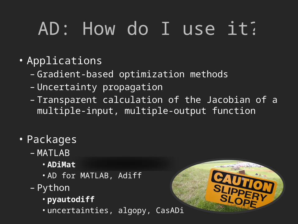
AD: How do I use it?

• Applications– Gradient-based optimization methods– Uncertainty propagation– Transparent calculation of the Jacobian of a multiple-input,

multiple-output function

• Packages– MATLAB

• ADiMat• AD for MATLAB, Adiff

– Python• pyautodiff• uncertainties, algopy, CasADi

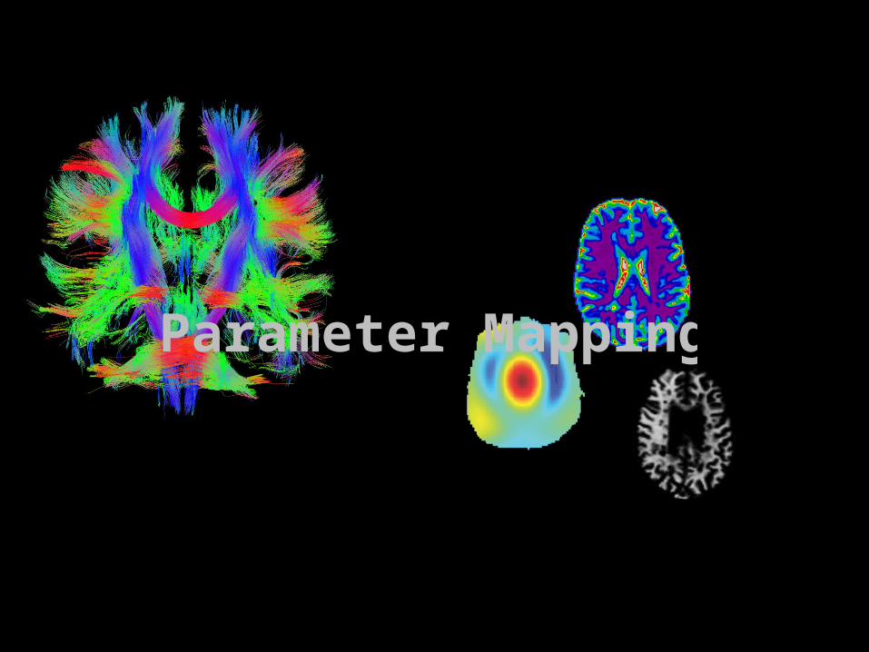
Parameter Mapping

What is Parameter Mapping?

1. Start with a signal model for your data2. Collect a series of scans, typically with only 1

or 2 sequence variables changing3. Fit model to data

• Motivation– Reveals quantifiable physical properties of tissue

unlike conventional imaging– Maps are ideally scanner independent

Parameter Mapping

• Some examples– FA/MD mapping with DTI – most widely known

mapping sequence– T1 mapping – relevant in study of contrast agent

relaxivity and diseases– B1 mapping – important for high field applications

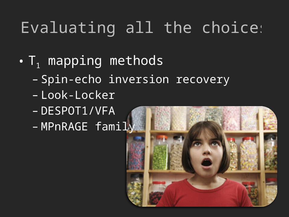
Evaluating all the choices

• T1 mapping methods– Spin-echo inversion recovery– Look-Locker– DESPOT1/VFA– MPnRAGE family

Evaluating all the choices

• T1 mapping methods– Spin-echo inversion recovery– Look-Locker– DESPOT1/VFA– MPnRAGE family

DESPOT1 T1 Mapping

• Protocol optimization– What is the acquisition protocol which best

maximizes our T1 precision?

Christensen 1974, Homer 1984, Wang 1987, Deoni 2003

𝑆𝑆𝑃𝐺𝑅 (𝛼 ,𝑇𝑅 )∝𝑀 01−𝑒−𝑇𝑅 /𝑇 1  

1−cos (𝛼 )𝑒−𝑇𝑅/𝑇1

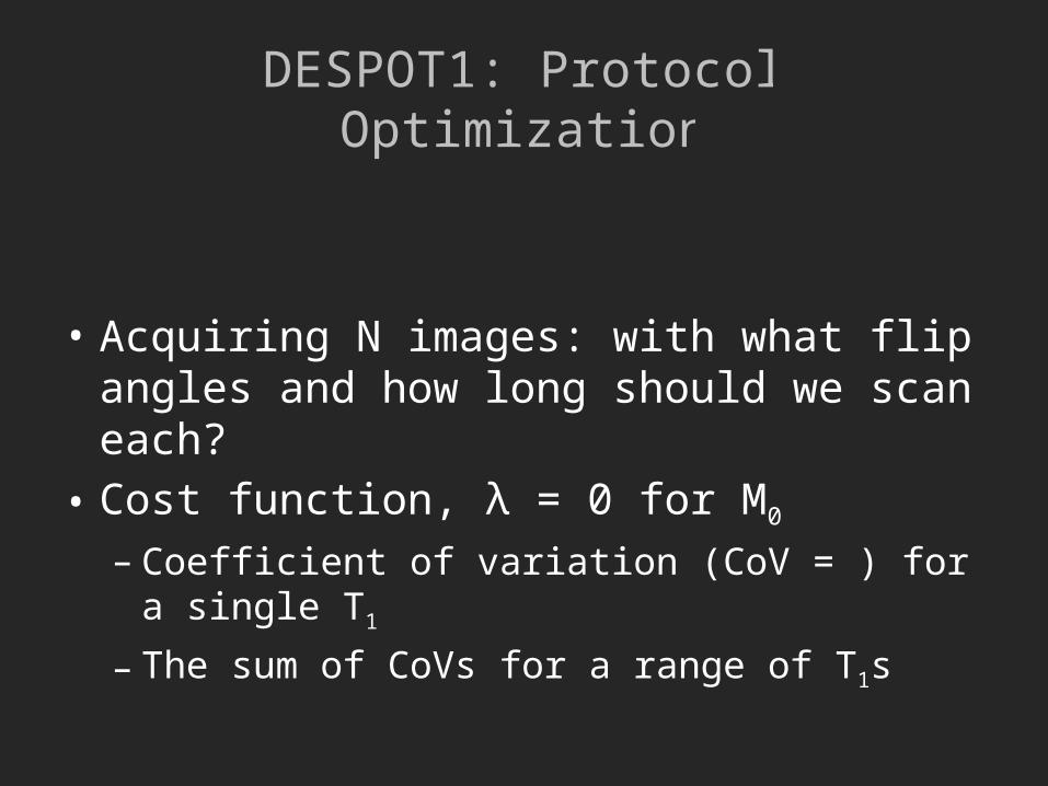
DESPOT1: Protocol Optimization

• Acquiring N images: with what flip angles and how long should we scan each?

• Cost function, λ = 0 for M0

– Coefficient of variation (CoV = ) for a single T1

– The sum of CoVs for a range of T1s

Problem Setup

• Minimize the CoV of T1 with Jacobians implemented by AD

• Constraints– TR = TRmin = 5ms

• Solver– Sequential least squares programming

with multiple start points(scipy.optimize.fmin_slsqp)

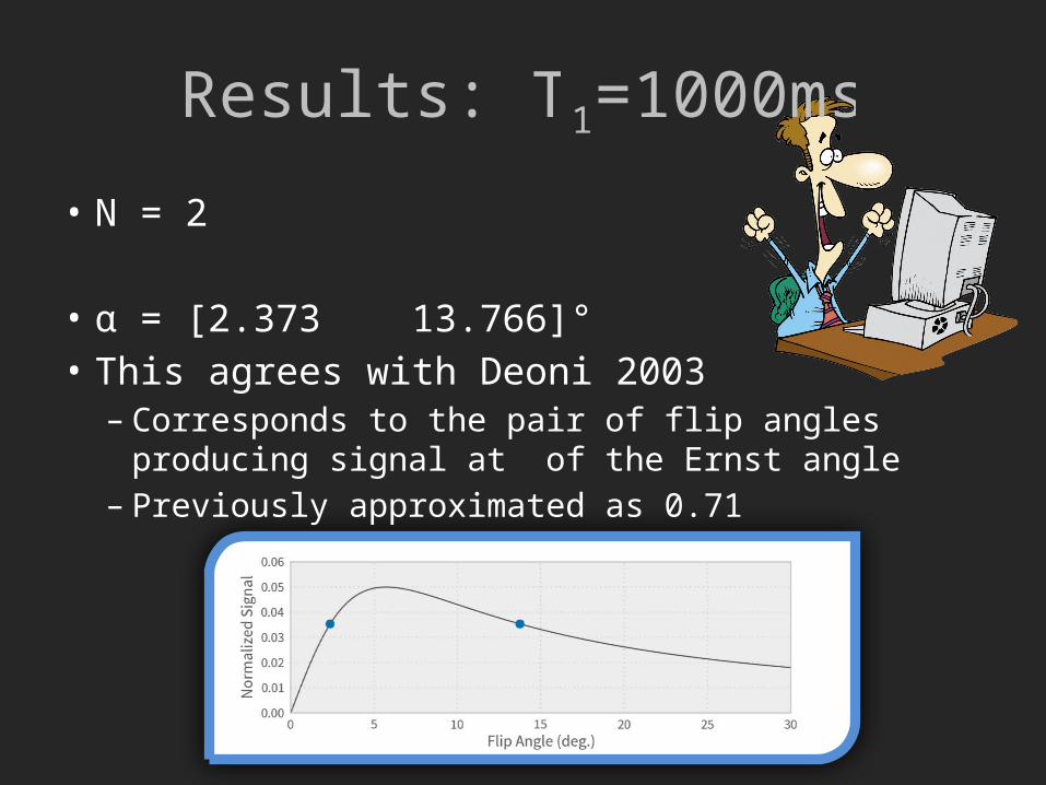
Results: T1=1000ms

• N = 2

• α = [2.373 13.766]°• This agrees with Deoni 2003

– Corresponds to the pair of flip angles producing signal at of the Ernst angle

– Previously approximated as 0.71

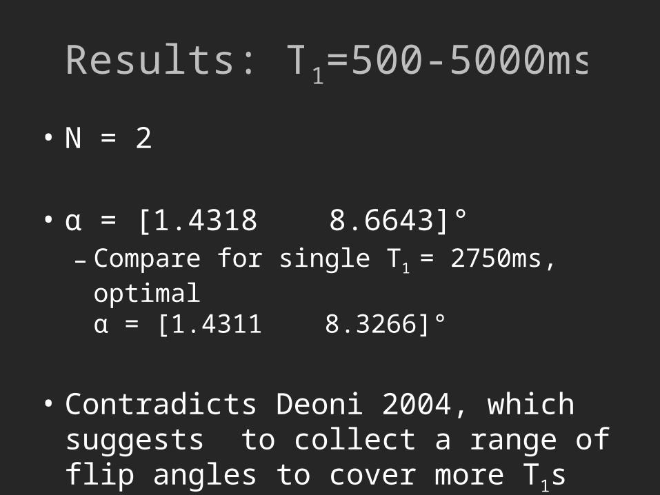
Results: T1=500-5000ms

• N = 2

• α = [1.4318 8.6643]°– Compare for single T1 = 2750ms, optimal

α = [1.4311 8.3266]°

• Contradicts Deoni 2004, which suggests to collect a range of flip angles to cover more T1s

Results: T1=500-5000ms

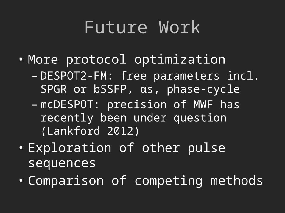
Future Work

• More protocol optimization– DESPOT2-FM: free parameters incl. SPGR or bSSFP,

αs, phase-cycle– mcDESPOT: precision of MWF has recently been

under question (Lankford 2012)• Exploration of other pulse sequences• Comparison of competing methods

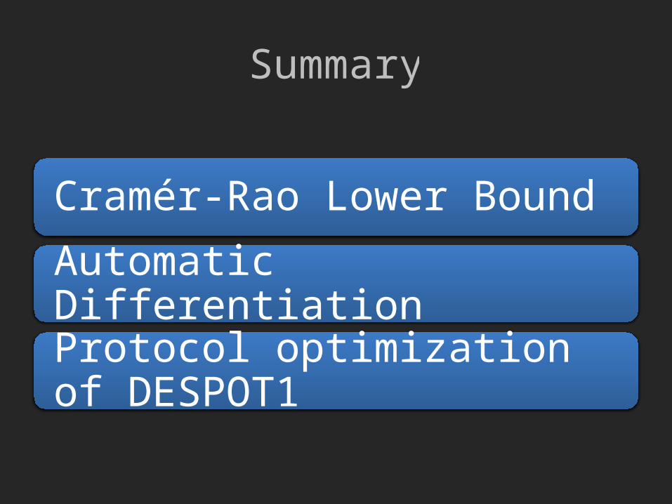
Summary

Cramér-Rao Lower Bound

Automatic Differentiation

Protocol optimization of DESPOT1

Questions?

• Slides available athttp://mr.jason.su/

• Python source code available soon